applying hydrogeological methods and hubbert’s force ...2_-_letter.pdf · much upon hubbert’s...
TRANSCRIPT

Applying Hydrogeological Methods and Hubbert’s Force Potential to Carbon Storage: A Primer
by
K. Udo Weyer, Ph.D., P.Geol., P.HG. WDA Consultants Inc., Calgary, Alberta, Canada
Part 1: Introduction and Explanations
Foreword 2 Summary 2 Key Points 4 Arrangement of Slideshow 9 Section Highlights 11 Conclusions 17 Credits 19 List of References 21
Part 2: Slides [two per page]
June 24, 2009 with corrections April 10, 2010 and Nov 27, 2014
© 2009 K.U.Weyer
page 2
Foreword
WDA’s involvement in Carbon Sequestration started in August, 2008 when Dr. Weyer got an invitation by the Brazilian oil company Petrobras to present on the application of physics-based groundwater dynamics to carbon storage at a Salvador Seminar. It did not take long to find that the physics-based approach is an essential addition to methods applied so far to carbon storage. The physics-based methods of this primer will significantly increase the probability of avoiding unpleasant surprises that might come along if only reservoir engineering methods were used in the grand scale that worldwide carbon sequestration requires. All quoted papers on physical matters have been peer-reviewed within journals or under a review contract (as was the case with the paper Weyer, 1978). When delivering a Powerpoint presentation at the Geofluids seminar of the Canadian Society of Petroleum Geologists (CSPG) on December 1st, 2008 in Calgary, a lively and in-depth discussion ensued on the matter of ‘buoyancy forces’. Several participants found it difficult to accept that under hydrodynamic conditions the so-called ‘buoyancy forces’ would diverge from the vertical direction. It became clear that the matter of ‘buoyancy forces’ constitutes a major stumbling block in accepting Hubbert’s (1940, 1953, 1957, 1969) derivation of force potential and force fields. Because of this reason we decided to write highlights for all sections and additional explanations for the attached Powerpoint slideshow. Additional slides were added to the buoyancy subsection to shed light on the dependence of the so-called ‘buoyancy forces’ upon pressure potential forces under both hydrodynamic and hydrostatic conditions. In fact, it is the case that the directions of the fresh water pressure potential gradients determine the direction of the so-called ‘buoyancy forces’ under both hydrostatic and hydrodynamic conditions. It so happens that the pressure potential forces are directed vertically-upward under hydrostatic conditions, but may take any direction in space under hydrodynamic conditions. The written text and the slideshow have been divided into sections by topics, and thus provide a guide for the reader to study the topics of particular interest. We recommend, however, that the reader follow the logical sequence of all topics.
Summary
The long term fate and leakage of CO2 injected into geological formations depends as much upon Hubbert’s mechanical Force Potentials for fluid flow in the subsurface (Hubbert, 1940) as upon the geologic structures. These force fields of Hubbert’s Force Potential [energy/unit mass] are created within fresh groundwater in response to gravitational energy omnipresent in the subsurface. Forces within other fluids, such as salt water, oil, gas, and CO2, are derived from the energy field of the fresh groundwater. Hubbert’s force fields were applied in developing the Theory of Groundwater Flow Systems (Tóth, 1962, 2009, Freeze and Witherspoon, 1966, 1967). These flow systems penetrate into similar depth ranges as the injection of CO2. In areas of regional downward flow, the groundwater flow systems may cause ‘buoyancy reversal’, a term created by Weyer (1978), in low-permeable layers (aquitards and

page 3
caprocks). ‘Buoyancy reversal’ means that under certain geologic and hydrodynamic conditions in the subsurface, the so-called ‘buoyancy force’ (i.e. the pressure potential force) is directed downwards. These conditions have frequently been encountered in Alberta, Canada and in other areas. In general, under hydrodynamic conditions in the subsurface, the so-called ‘buoyancy force’ may be directed in any direction in space. These directions are determined by the directions of the pressure potential forces in the Force Potential field of fresh groundwater. Only under hydrostatic conditions is the so-called ‘buoyancy force’ (i.e. the pressure potential force) always directed vertically upwards. After Hubbert’s (1940) Force Potential had been proven physically correct, its application within the petroleum industry was simplified to allow the continued application of velocity potential for fluid flow calculations by incorrectly relating the energy to the volume [energy/unit volume], not to the mass [energy/unit mass]. As a consequence, these simplifications led to such invalid assumptions as
‐ water to be incompressible,
‐ the fluid flow would be driven by pressure and follow the direction of the pressure gradients,
‐ the fluid flow would, for all practical purposes, be concentrated in aquifers and fault systems,
‐ seepage to the surface could only occur where aquifers or fault systems connect to the surface or to shallow groundwater systems, barring leakage through boreholes,
‐ the belief that fluids of densities > 1 g/cm3 would remain at greater depth within the geologic layers,
‐ the belief that hardly any fluid passes through aquitards, while in reality, under natural conditions, often twice as much fluid passes through the overlying aquitards as through the underlying aquifer, and
‐ the isolated occurrence of up-dip and down-dip flow of fluids isolated within deep aquifers; again, this concept does not conform to the physics of Hubbert’s (1940) Force Potential and Tóth’s (1962) Theory of Groundwater Flow Systems.
The application of the principles of Hubbert’s Force Potential to carbon sequestration is fundamental in achieving realistic results in any modelling attempt. In this author’s view, the IPCC’s attempt (Intergovernmental Panel on Climate Change, 2005, Fig. 5.8) to determine a 1000 year buoyancy-driven migration of CO2 is seriously flawed as it ignores gravitational and pressure potential forces occurring within regional groundwater force fields. Similarly, Fig 5.25 (ibid.) is too much an over-simplification for its concepts to be applied at any realistic site investigation. The additional application of Hubbert’s Force Potential, Tóth’s Groundwater Flow Systems, and of hydrogeological monitoring methods will significantly improve the predictability of the behaviour of sequestered CO2. What is generally missing from the treatment of this topic is the consideration of deeply-penetrating regional groundwater flow systems and its consequences using the principals of Hubbert’s Force Potential. These points of view are illustrated with examples from the literature, with field studies, and with the results of mathematical modelling. Any risk analysis on carbon sequestration and subsequent leakage needs to
page 4
consider fluid flow analysis based on the principles of Hubbert’s Force Potential and Tóth’s Theory of Groundwater Flow Systems. Any application of hydrostatic ‘buoyancy forces’ (i.e. vertical pressure potential forces) in a hydrodynamic environment is erroneous. The application of Muskat’s (1937) velocity potential (slide 17) is also incorrect even if the second term attempts to include gravitational forces in an “awkward” (Payne et al., 2008, p.53) manner.
Key Points
For ease of orientation into the complex matters dealt with, the key points summarize key additions to the carbon storage methods applied so far in CCS. They are:
Key Point 1: Limitations of the IPCC (2005) approach
Key Point 2: Velocity Potential vs Force Potential
Key Point 3: Regional gravitational flow of groundwater
Key Point 4: Water penetrates caprocks
Key Point 5: Regional permeabilities systemically exceed measurements in karstic and fractured rocks
Key Point 6: Oil field pumping creates subsidence and fractures in caprocks and aquitards
Key Point 7: Hydraulic windows depend upon contrasts of permeability, and are not limited to high permeabilities
Key Point 8: Salt water moves upwards towards discharge areas
Key Point 9: Omnipresent ‘buoyancy forces’ (i.e. vertical pressure potential forces) exist under hydrostatic conditions only
Key Point 10: ‘Buoyancy Reversal’ may occur in aquitards and caprocks
Key Point 11: Carbon monitoring also to be done using hydrogeological methods
Key Point 12: Presently-available computer codes and simulators need re-writing for CO2 storage.
page 5
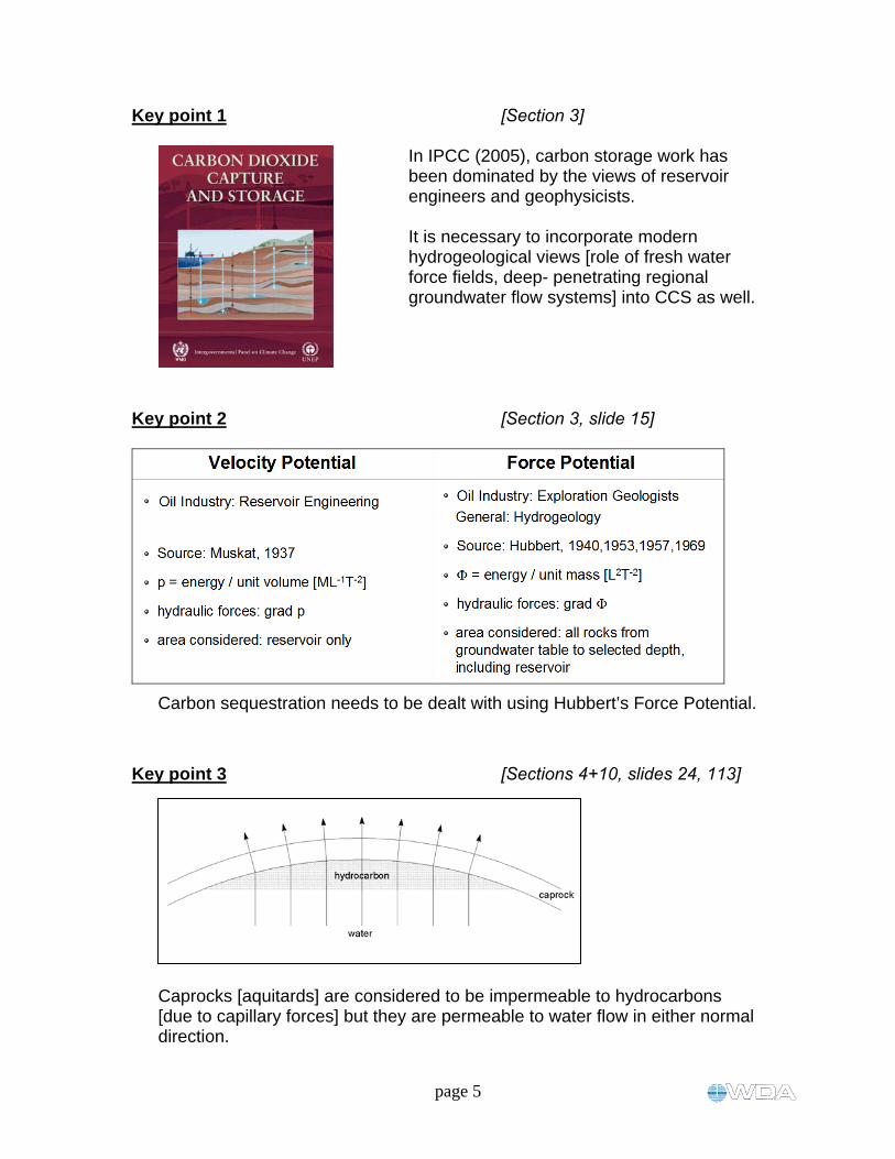
Key point 1 [Section 3]
In IPCC (2005), carbon storage work has been dominated by the views of reservoir engineers and geophysicists. It is necessary to incorporate modern hydrogeological views [role of fresh water force fields, deep- penetrating regional groundwater flow systems] into CCS as well.
Key point 2 [Section 3, slide 15]
Carbon sequestration needs to be dealt with using Hubbert’s Force Potential.
Key point 3 [Sections 4+10, slides 24, 113]
Caprocks [aquitards] are considered to be impermeable to hydrocarbons [due to capillary forces] but they are permeable to water flow in either normal direction.

page 6
Key point 4 [Section 5, slide 34]
Regional permeabilities of fractured or karstic rocks are often 2 to 4 orders of magnitude larger than permeabilities measured in well tests.
Key point 5 [Section 5, slide 35]
Pumping in oil or gas fields creates stress-induced fractures in caprocks and aquitards due to subsidence. Injection of CO2 will cause heave, thus rejuvenating previously-created subsidence-related fractures and possibly creating new ones
Key point 6 [Section 6, slides 58, 97]
Regional gravitational flow of groundwater creates the force fields determining the flow directions of hydrocarbons and CO2 in the subsurface.
page 7
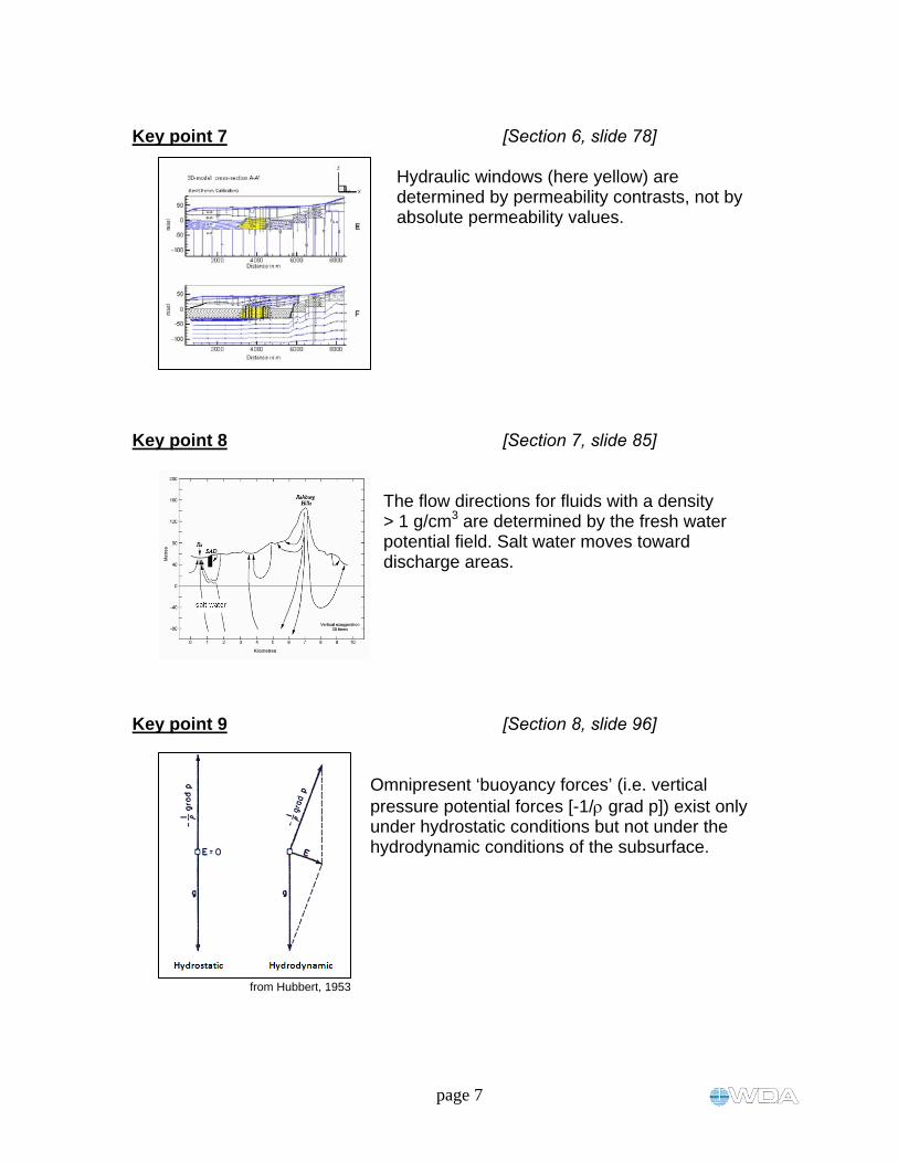
Key point 7 [Section 6, slide 78]
Hydraulic windows (here yellow) are determined by permeability contrasts, not by absolute permeability values.
Key point 8 [Section 7, slide 85]
The flow directions for fluids with a density > 1 g/cm3 are determined by the fresh water potential field. Salt water moves toward discharge areas.
Key point 9 [Section 8, slide 96]
Omnipresent ‘buoyancy forces’ (i.e. vertical pressure potential forces [-1/ grad p]) exist only under hydrostatic conditions but not under the hydrodynamic conditions of the subsurface.
from Hubbert, 1953

page 8
Key point 10 [Section 9, slide 100]
‘Buoyancy Reversal’
The so-called ‘buoyancy forces’ (i.e. pressure potential forces [-1/ grad p]) can be directed downwards in aquitards (caprocks) thus hindering the upward migration of hydrocarbons and CO2.
Key point 11 [Section 10, slide 114]
Monitoring systems for carbon storage applied to date concentrate mainly on geophysics, and have missed the hydraulic methods of hydrogeology.
Key point 12 [Section 10]
Due to widespread and erroneous assumption of ‘buoyancy forces’ (i.e. vertical pressure potential forces) and its incorporation in computer simulation codes, these codes need to be rewritten for CCS work to reflect the pressure potential forces in fresh groundwater force fields in determining the directions and migration times for CO2 flow.
page 9
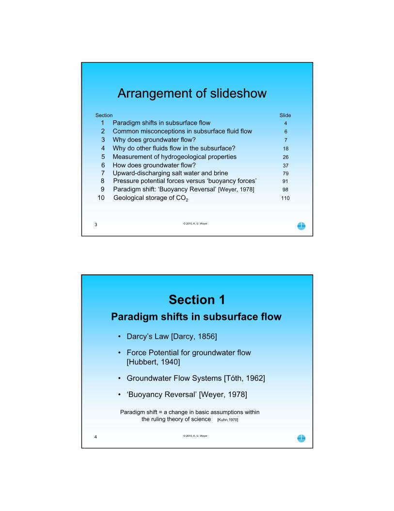
Arrangement of Slideshow
This list helps to locate any particular slide in the slideshow and allows the reader to choose a section that he would like to concentrate on.
Section Contents Slide
1 Paradigm shifts in subsurface flow ….………..................................................... 4
2 Common misconceptions in subsurface fluid flow ………………………............. 6
3 Why does groundwater flow? ............................................................................. 7 • Paradigm Shift: Darcy Equation 8 • Laplace Equation 9 • Paradigm Shift: Force Potential 10
• Velocity Potential 17
4 Why do other fluids flow in the subsurface? ....................................................... 18 • Role of fresh water force fields 19 • Capillary forces 22
5 Measurement of hydrogeological properties .................…….…….............…..... 26 • Hydraulic, gravitational and pressure potential heads 27 • Piezometer nests 28 • Permeability units and conversion 29 • Range of permeabilities in various rocks 33 • Permeability dependence on scale of measurements 34 • Increase of permeability due to subsidence and heave 35 • Porosity 36
6 How does groundwater flow? ............................................................................ 37 • Paradigm Shift: Hubbert, 1940: Force Potential 38
• Hubbert’s theoretical approximation of groundwater flow between two valleys 38
• Sand model of groundwater flow and 2D-vertical mathematical model [1] 39
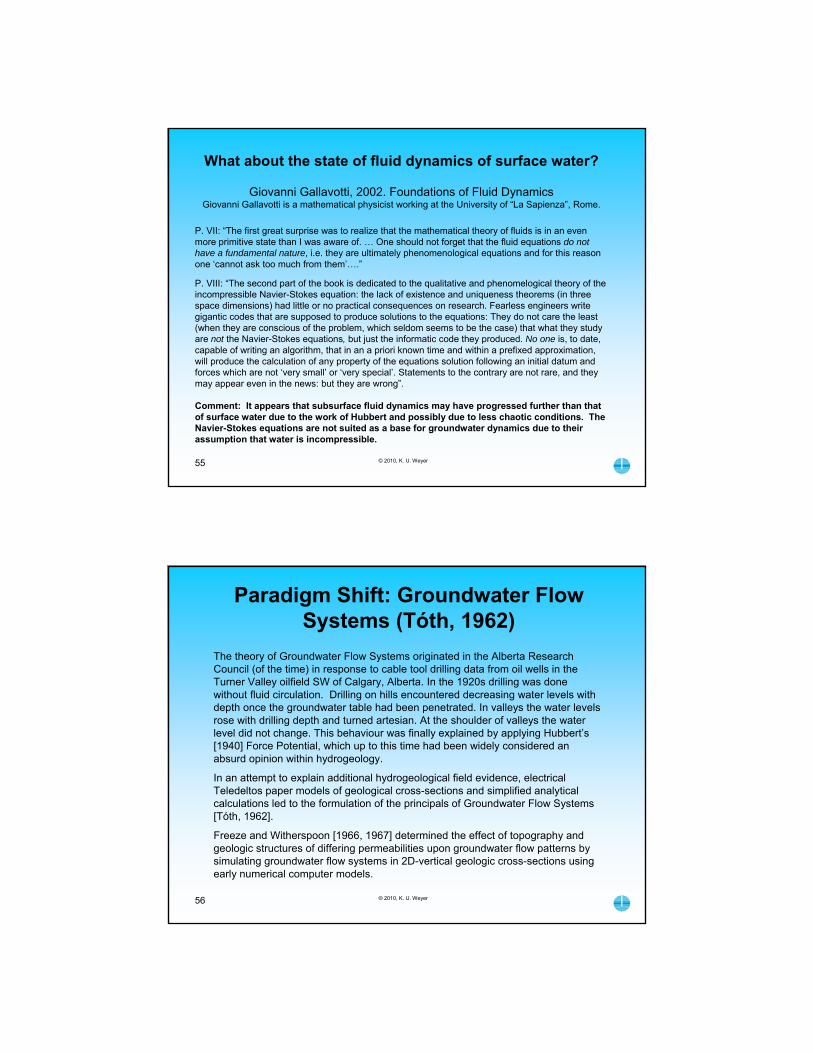
• Counterplay of forces 40 • Paradigm Shift: Tóth, 1962: Groundwater Flow Systems 56
• Field example: Turner Valley, Alberta 57 • Mathematical model [2] by Tóth [1962] 58 • Mathematical models [3] by Freeze and Witherspoon [1967] 59 • Continuity of flow between aquitard and aquifer 61 • Field example France: How to see groundwater flow systems
penetrate aquitards 63 • Erroneous assumptions about regional groundwater flow 66 • Field example and 2D-vertical mathematical model [4]:
Brake landfill in Germany 69 • Silt [10-8 m/s, 1 mD] as an efficient hydraulic window 75
• Field example and 3D-mathematical model [5]: Düsseldorf/Hilden, Germany 75

page 10
Section Contents Slide 7 Upward-discharging salt water and brine ........................................................... 79
• Field example and mathematical model [6]: Upward discharge from depth of 1000 m of ocean-type saline water at Münchehagen, Germany 80
• Field example Salt River Basin, NWT, Canada: Upwards discharge of saturated brine 88
• Field example Great Slave Lake, NWT, Canada: Upwards discharge of saline water 89
8 Pressure potential forces versus ‘buoyancy forces’ (a misnomer)...................... 91 • Pressure potential forces (‘buoyancy’) under hydrostatic conditions 92 • Reason for change of magnitude of pressure potential forces of
salt water, oil, gas, and CO2 from that of fresh water 94 • Comparison of pressure potential forces under hydrostatic and
hydrodynamic conditions 95 • Differing flow directions for fresh water, oil, and gas within the same
fresh water force field 97
9 Paradigm Shift Weyer, 1978: ‘Buoyancy Reversal’ ........................................... 98 • Theory 99 • Field example: Swan Hills, Alberta 102
10 Geological storage of CO2 …….....…….……………………………..................... 110 • Sink conditions versus source conditions 111 • Mathematical models by IPCC [7] and Princeton [8] 115 • Effect of deep wells upon fluid flow 118
• Microannuli 122 • Deep well abandonment 126
• Field examples and mathematical models 128 • Field example and mathematical model [9]: Hayter field,
Provost area, Alberta 128 • Field example and mathematical model [10]: Freed
investigation, TWP 50-51, Rge 14-15 W4M Alberta 132

page 11
Section Highlights
The section highlights help to convey the framework for the topics dealt with therein. It helps the reader to peruse the topics that are of particular interest.
1. Paradigm shifts in subsurface flow
Shows the essential improvements in dealing with subsurface flow, the ‘new scientific truths’. Explains why these improvements are almost never accepted by contemporary scientists and practitioners.
2. Common misconceptions in subsurface fluid flow Lists stumbling blocks delaying and preventing understanding of the physical processes governing fluid flow in the subsurface
3. Why does groundwater flow? Explains the essential and basic equations dealing with groundwater flow and their proper use from the viewpoint of physics. The sole application of pressure gradients as driving forces is inadequate and leads to incorrect flow directions, volume and velocities, as does the application of velocity potentials under anisotropic and/or heterogeneous conditions..
4. Why do other fluids flow in the subsurface? Fresh groundwater (density 1 g/cm3) determines the energy field for all fluids in the subsurface. Therefore directions of pressure potential forces ([-grad p]/ρ) for all subsurface fluids follow the pressure potential force directions of the fresh water albeit their magnitude is different, either larger when the density ρ <1 g/cm3 (oil, gas, CO2) or smaller when that fluid’s density ρ>1 g/cm3 (salt water, brine).
Hence the pressure potential force directions of all fluids in the subsurface are dependent on the geometry of the pressure potential force fields of fresh groundwater. What is different are the flow directions of the individual fluids due to the effect of vectoral addition of the differing magnitudes of the pressure potential forces with the gravitational force g. These differences in resultant flow directions may be large (slides 21 and 97) or small (slide 87).
Capillary pressure potential forces are mechanical forces and are also taken into account by vectoral addition. Their direction and magnitude is, however, not determined by the geometry of pressure potential force fields of fresh groundwater but by the geology and the steepest rate of increase of the grain size of the sediment (Hubbert 1953, p.1977). The force will be pointing in the direction of this steepest increase of grain size change if preferentially water-wet or in the opposite direction if preferentially oil-wet or CO2-wet.
5. Measurement of hydrogeological properties This section summarizes the determination, ranges and comparison of basic hydraulic properties such as heads, porosity, the various permeability units and their meaning, as well as the dependence of resulting permeabilities upon the scale of measurements (core, well tests, regional) and subsidence occurring during pumping of oil and gas fields. It turns out that it is nearly impossible to determine the actual
page 12
regional permeability of fractured or karstic rocks by direct measurement and that this regional permeability could be several orders of magnitude higher than the permeabilities measured in the field (slide 34). Slide 35 shows the principle of the creation of fractures due to subsidence. For the deep Dutch gas fields (pumping from about 3000 m depth from fractured rocks) a total surface subsidence of 1 m is expected to occur. The total movement in the immediate ‘caprock’ would be larger by an unknown amount leading to the formation of fractures related to stress changes. These fractures may be permeable to CO2. Injection of CO2 will cause heave and thereby rejuvenate subsidence-induced fractures and possibly create new ones. Formation of fractures will be indicated by micro-seismic events.
6. How does groundwater flow? This section presents the various physical fields and their application in determining the flow pattern of fluids in the subsurface and is here divided into subsections.
Paradigm Shift Hubbert, 1940: Force Potential
First Hubbert’s famous 1940 cross-section of groundwater flow between two valleys is shown and the concept of recharge and discharge areas is explained. Under hills, the flow is downward into the groundwater body (recharge area); under valleys, the flow is upward leaving the groundwater body into surface water bodies or evaporation (discharge area). Because of upward flow these discharge areas usually display artesian (flowing) conditions. Slides 40 to 42, from animations of a real table-sized sand model of a geologic cross-section (animation available on-line at http://www.wda-consultants.com/page20.htm) shows the same kind of flow pattern with recharge and discharge areas, and artesian flow in the discharge area. The flow patterns in the sand model are then successfully mathematically simulated in a vertical cross-section (slide 47) using permeability contrasts instead of actual permeability measurements.
Counterplay of forces
Mechanical force fields (the gradients of energy fields) drive all fluid flow in the subsurface in response to the gravitational energy. At the groundwater table the pressure potential energy is practically zero, when neglecting forces within the unsaturated zone. At this point, all the energy of the unit mass consists of gravitational energy. Any downward movement in the gravitational field frees a large amount of energy which is used to overcome the resistance to flow exerted by the rocks penetrated. The amount not used in overcoming this resistance to flow is stored within the unit mass as deformation (compression) of the unit mass. Water is slightly compressible and can store an extraordinary amount of energy when compressed. This stored energy is released when the water flows upward against the gravitational gradient and overcomes the resistance of the rock penetrated.
In slide 55, the application of the non-physics-based incompressible Navier-Stokes equation for surface water hydrodynamics is shown to be an phenomenological equation only. This equation should not be applied to fluid flow calculations in subsurface conditions nor should Muskat’s (1937, eq. 3.3(3)) velocity potential equation even if it attempts to include gravitational forces (ibid., p.132) in an “awkward” (Payne et al., 2008, p.53) manner

page 13
Paradigm Shift Tóth, 1962: Groundwater flow systems – they penetrate that deep?
The use of vertical cross-sectional groundwater flow models has been pioneered by Tóth (1962) and Freeze and Witherspoon (1966, 1967) to arrive at the Theory of Groundwater Flow Systems and to document the effect of topography and geological structures on groundwater flow pattern. The authors elucidate the determinant role of the topography of the groundwater table and of the geological structures on the distribution of recharge and discharge areas as well as upon the pattern and depth range of groundwater flow systems.
Tóth (1962) showed how an undulating groundwater table (amplitude 15 m; total slope 125 m over 6 km) caused, in homogeneous and isotropic rocks, groundwater flow systems to penetrate to 3000 m depth. Tóth (2009), in a new book on gravitational systems of groundwater flow, while summarizing much of the present knowledge of the principle pattern of groundwater flow systems and their effect on geological processes, shows these systems to penetrate to depths of 5 km or more.
Freeze and Witherspoon (1966, 1967) used a dimensionless variable, S, for length and depth of the cross-sections used for simulating groundwater flow. This means that at a length of 10 km, the depth of flow would have been 1 km; at a length of 50 km, the depth of flow would have been 5 km deep. These limitations have been created by the choice of the length-to-depth ratio for the model, not by physical constraints.
It was thus shown that flow systems would penetrate to several kilometers depth and that, under natural conditions, more than twice as much water would flow through an overlying aquitard into and out of an underlying aquifer as was actually flowing within the aquifer (slides 59 [2] and 60 [2]). Weyer (1996) showed the ease with which one can visualize the actual upward and downward flow directions in an aquitard by comparing water levels in the buried aquifer with those at the groundwater table (slides 62 and 65). The additional example of 2D-vertical groundwater flow models [4] and [6] shows the groundwater flow in recharge areas penetrating deeply through clay layers (aquitards, aquicludes) into higher permeable layers and upward flow through the same layers to the discharge area at the surface [slides 73 and 83].
Silt [10-8 m/s, 1 mD] as an efficient hydraulic window
It is often assumed that, in the subsurface, hydraulic windows need to be highly permeable to be effective conduits for migration of groundwater. The field example and 3D-mathematical model [5] Hilden/Düsseldorf shows otherwise. The model simulated flow through a silt window that is surrounded by clay. A head difference of 15 m (from the groundwater table to the underlying Devonian dolomite layers) and a permeability difference of about 1 order of magnitude in the aquitard layer was sufficient to draw much of the groundwater downwards into a higher-permeable layer of Devonian dolomite and from there towards a dewatering mine.
The example illustrates in which way permeability contrasts exert a forging influence on force fields and resulting flow directions in the subsurface.
page 14
7. Upward-discharging salt water and brine Many scientists and practitioners believe that salt water and brine would move to the bottom of groundwater flow systems and stay there as they could not move upwards due to the density differences. The mechanism assumed to be at work is also hydrostatic but opposite in effect to the upward-directed hydrostatic ‘buoyancy’ for fluids with a density < 1 g/cm3. Many computer codes have been written with the assumption that hydrostatic conditions apply to flow of salt water and brine when they actually behaved differently under hydrodynamic conditions. Again the hydrostatic concept of flow does not reflect reality.
The field example and mathematical model [6] Münchehagen landfill in Germany showed the salt water flow pattern (density of ocean water) to be practically the same as that of fresh groundwater (slide 87). The system was of variable density in that recharged fresh groundwater picked up its salt load in marl with evaporitic parts at about 1000 m depth. Then it flowed upwards towards the landfill and turned at about 50 m depth towards the discharge area at the river Ils (slides 83 and 85). This result of the mathematical model was confirmed by salinity measurements in borehole 226 (slide 86). The results of the mathematical model were based on geology taken from public geologic maps in the scale 1:25,000 and were obtained in the first model run.
The second field example shows upward discharging saturated brine within the Salt River catchment basin, NWT, Canada (slide 88). There have to exist very high upward-directed fresh groundwater gradients. To overcome the gravitational force the freshwater pressure potential gradient needs to be >1.3 • g (the gravitational force).
The third field example also stems from the Western Canadian Sedimentary Basin which contains several salt layers at depth. It shows salty water discharging at the southern shore of Great Slave Lake (slide 89). The investigation of this flowing borehole was part of a multi-year study dealing with the dewatering at Pine Point Mines.
8. Pressure potential forces versus ‘buoyancy forces’ (a misnomer) There exists considerable confusion about the mechanism causing buoyancy under hydrostatic and under hydrodynamic conditions. In fact most, if not all, scientists and practitioners assume that the so-called ‘buoyancy force’ is directly dependant on differences in density only and is vertically directed upward in both hydrostatic and hydrodynamic conditions. Both assumptions are physically incorrect.
The hydrostatic conditions are a special case of hydrodynamic conditions whereby there is no flow occurring within the energy field created by gravitation within the water body. In fact the energy state throughout the hydrostatic water body is equivalent and no water flows. At all locations within the hydrostatic water body pressure potential gradients (forces) are equal to the gravitational gradient (force) and cancel each other as they are opposite in direction. Slide 93 shows the mechanism how the pressure potential force of the water is the vehicle to create upward-directed forces for less dense fluids (C:oil, D:gas) and downward-directed for denser fluids (A: salt water). On the right hand side of the hydrostatic slide 93 the

page 15
pressure potential forces for water, oil, and gas have been combined into one vector diagram showing how the upward forces for lighter material are created in the energy field of the water. Under hydrostatic conditions the combined vector diagram shows a vertically-upward direction; under hydrodynamic conditions it does not (slide 95).
Slide 95 enforces that the generally non-vertical direction of the pressure potential gradient under hydrodynamic conditions necessarily implies that the pressure potential gradients for oil, gas, CO2, salt water and brine are directed in the same direction as that of the fresh groundwater water due to the physical processes at work in the subsurface. The pressure potential gradients for oil, gas, CO2, salt water and brine are therefore not vertical under hydrodynamic conditions. The actual flow directions are then determined by vectoral addition for each of the fluids as shown in slide 97.
In general, under hydrodynamic conditions in the subsurface, the so-called ‘buoyancy force’ may be directed in any direction in space. Only under hydrostatic conditions is the so-called ‘buoyancy force’ (i.e. the pressure potential force) always directed vertically upwards. The use of the term ‘buoyancy force’ has been misleading many scientists and practitioners and should be discontinued. The same hydrodynamic principle also applies to horizontal flow. There, the gravitational gradient is directed vertically downward, and by necessity the pressure potential gradient (force ) is directed obliquely upwards in the direction of the horizontal flow. Typically that point is missed on presentations of model calculations as for example those presented at the GHGT9 and by the Princeton model [8] (slide 117). In fact, to our knowledge, there doesn’t yet exist any model code which attempts to include the pressure potential force in a physically-correctly manner when calculating flow directions for oil, gas and CO2. Existing model codes assume vertical hydrostatic conditions for what they call ‘buoyancy force’. That needs to be corrected when dealing with the grand scale of CO2 sequestration.
9. Paradigm shift: ‘Buoyancy Reversal’ [Weyer, 1978] In areas with strong downward flow, the need to maintain the downward flow through ‘aquitards’ may have to balance its energy needs from the compressed unit mass if the gravitational energy gain (due to decrease in elevation) is not sufficient to maintain the necessary flow rate. Under these conditions, the pressure in the aquitard decreases with depth. These aquitards would then show a ‘Buoyancy Reversal’, a term created by Weyer (1978). ‘Buoyancy Reversal’ means that under these geologic and hydrodynamic conditions in the subsurface, the pressure potential force (the so-called ‘buoyancy force’) is directed downwards. These conditions have frequently been encountered in the Swan Hills area in Alberta and in other areas worldwide
10. Geological storage of CO2 The first part of this section deals with the change within an oil reservoir from hydraulic sink conditions during production pumping to hydraulic source conditions as CO2 is injected (slide 112). Within CCS activity, hydraulic monitoring would track the effect of these changes within the surrounding rocks (slide 114).

page 16
The second part of this section points out some shortcomings in the manner mathematical models have been applied to date to predict the migration behaviour of large scale CO2 sequestration. The models shown ignore the physically-derived force fields in the subsurface. Instead one considers the hydrostatic “buoyancy force” (i.e. a vertical pressure potential force), and capillary pressure (slide 116) while the other considers hydrostatic conditions and horizontal flow by pressure gradients only (slide 117).
The third part of this section visualizes the omnipresence of boreholes in mature basins of North America and other continents. The abandonment procedures usually have been imperfect, leading to leakage problems for large scale CO2 sequestration and its associated long term rise of pressure potentials. In spite of statements to the contrary, this is a situation not yet experienced when injecting fluids in parts of operating oil fields. We are confronted with a situation necessitating unbiased and encompassing treatment of the problem and risk assessments applied. Oil field operation has lowered the pressure potentials by the equivalent of many hundred meters of freshwater head (slides 112 and 123) and thereby created sinks for regional groundwater flow in the subsurface. With large scale CO2 injection, these sinks will be turned into sources by increased pressure potential forces resulting in changed flow patterns in the subsurface. In this environment the role of microannuli will most likely be significant. The example calculation of downward fluid flow through microannuli (slide 124) has been based on actual head differences at Alberta well 8-16-41-1 (slide 123), assumptions about the opening width and vertical extent of the microannuli, and equations used within the oil industry.
The fourth part of this section communicates the results of 2D-vertical fresh groundwater flow models within geologic cross-sections taken from the real world. The field example and mathematical model [9] was part of an investigation leading to the 1992 ERCB hearing on the Hayter Field near Provost, Alberta (slide 128). The model assumed existing wells in the recharge area and discharge area to be leaking. Upon restoring the pressure potential distribution to its original conditions slide 131 shows how natural flow from the recharge area would penetrate through leaking wells into the reservoir, flow through the reservoir to leaking wells located in the recharge area and discharge through these wells towards the surface. The transport from the reservoir to the discharge area would eventually happen without any addition of CO2 injection.
Field example and mathematical model [10] refers to an investigation in Central Alberta (slide 132). A farmer experienced salting of his water supply. The results of the mathematical model showed the changes in flow pattern of fresh groundwater which would be caused by the existence of one leaking well near the Vermillion River. The model made it conceivable that salt water had been migrating up from the reservoir into the farmer’s aquifer.
In general, partially abandoned wells create hydraulic shortcuts in aquitards above the sealed area of ‘caprocks’ and thereby considerably increase the overall regional permeability of the total aquitard system and also increase the amount of hydrous flow through caprocks.
page 17
Conclusions The conclusions are grouped under the headings Fluid flow, Capillary forces, Mathematical models, and Effect of well abandonment on CO2 sequestration. Fluid flow
• For CO2 sequestration, fluid flow in the subsurface should be dealt with using Hubbert’s (1940) Force Potential.
• Fluid flow in the subsurface is governed by mechanical fields created by fresh water. These fields are partially modified by raising the pressure potential at CO2 injection sites.
• Groundwater flow systems penetrate into the depths of deep well disposal.
• Groundwater flows in great amounts through aquitards and should be considered when dealing with CO2 sequestration.
• Saline water flows upwards into discharge areas, as did brines in the basin of the Salt River, NWT, Canada. Salt water does not segregate and sink to the bottom of the geologic system.
• Flow of ocean-type saline water can be modelled by fresh water models as the fresh water force field determines the general force directions.
• Operating CO2 sequestration sites should be monitored by a network of deep piezometer nests in addition to other methods.
Capillary forces
• Capillary forces should be dealt with in the manner described by Hubbert [1953].
• Capillary forces are capillary pressure potential gradients within non-hydrous fluids, not capillary pressure or capillary pressure gradients.
• Capillary forces at fluid interfaces should be determined in direct dependence upon the details of the sedimentary sequence between aquifers and aquitards and its geometry.
Mathematical models
• Mathematical models presented in IPCC [2005] and others do not take the force fields of gravitational Groundwater Flow Systems into account but should do so.
• Hydrodynamic model codes utilizing vertical ‘buoyancy forces’ instead of pressure potential forces are insufficient.
• Mathematical models making use only of pressure gradients and/or hydrostatic pressure are physically flawed, and lead to incorrect results in the direction, magnitude, and velocity of flow. They should be avoided.

page 18
• There is a need for modification of existing model codes to ensure full and simultaneous integration of gravitational, pressure potential and capillary forces.
Effect of well abandonment on CO2 sequestration
• The large number of existing oil wells pose a direct risk to CO2 sequestration due to widespread imperfect abandonment procedures.
• Risk assessments should consider all affected wells in a field and in nearby areas for leakage into and out of a reservoir. In North America the number of affected wells at sequestration sites often exceeds several hundred.
• Flow through microannuli in abandoned wells should be considered in any form of risk assessment for CO2 sequestration. Upward flow of CO2-saturated fluids through microannuli likely increases the corrosion of annulus cement significantly. In turn corrosion of annulus cement would increase the flow of CO2-saturated fluids significantly.
page 19
Credits
The work on the basics of hydrodynamics was originally supported directly or indirectly by
• the German Research Foundation [DFG], Bonn, Germany,
• the Centre d’Hydrogéologie a l’Université de Neuchâtel, Switzerland,
• the Hydrology Research Division [HRD] of the Canadian Federal Department of Environment, Ottawa, Canada, and,
• the hydrogeology and engineering geology sections of the Bureau de Recherches Géologiques et Minières [B.R.G.M.] in Orléans-la-Source [France]
Further development was done as an employee in the Hydrology Research Division [HRD] of Environment Canada in Ottawa and Calgary, and, for more than 20 years within my companies WDA Consultants Inc, Calgary, Canada and WKC Consultants, Krefeld, Germany. The Umweltbundesamt [German EPA] of the German Federal Department of Environment supported a research project on these matters, culminating in a German language report [Weyer, 1996] summarizing the basics of groundwater flow using Hubbert’s Force Potential and efficient methods for investigating deep-penetrating groundwater flow systems.
Ongoing discussions with James C. Ellis, WDA Consultants Inc., have been very helpful in re-testing and elucidating the physical validity of the concepts applied to carbon storage.
We are particularly indebted to the generosity of Petrobras and the scientific foresight of Dr. Paulo Cunha, Coordinator for CCS at the Petrobras R&D Center for the invitation to present at the 2nd Petrobras International Seminar on CO2 Capture and Geological Storage, 09-12 September 2008 - Salvador/BA – Brazil. The preparation for this seminar precipitated my ongoing involvement in carbon storage and the preparation of this primer.
This primer was also strongly influenced by papers presented and numerous discussions with participants at GHGT-9 (Washington D.C., November, 2008), the CO2 Geological Storage Modelling Workshop (Orléans, February 2009), the CO2GeoNet Open Forum (Venice, March 2009), the CO2 Risk Assessment Workshop (Melbourne, April 2009), the Wellbore Integrity Workshop (Calgary, May 2009), and the CO2 Monitoring Workshop (Tokyo, June 2009). Thanks is due to all the organizers of the above conferences, in particular the IEA GHG (Cheltenham, England) who organized the very informative workshops in Orléans, Melbourne, Calgary and Tokyo.
The ensuing discussions at 10 invited presentations of this material at scientific seminars, universities, and corporations in Brazil, Canada, Germany, the Netherlands, Australia and Japan also greatly helped to refine this primer and we are grateful to those who made this possible.
page 20
List of References [The references refer to Part 1 and 2.] Albinet, M., and S. Cottez, 1969. Utilisation et interprétation des cartes de
différences de pression entre nappes superposés. Chronique d'Hydrogéologie, Nr. 12, S.43–48, B.R.G.M., [Paris] Orléans
Celia, M.A., S. Bachu, J.M. Nordbotten, S.E. Gasda, and H.K. Dahle, 2004. Proceedings of the 7th International Conference on Greenhouse Gas Control Technologies (GHGT-7), vol. 1, p.663-672
Darcy, Henry, 1856. Les fontaines Publiques de la Ville de Dijon. Victor Dalmont, Paris.
de Vries, J.J., 2007. History of groundwater hydrology. Chapter 1 in J. W. Delleur, 2007. The Handbook of Groundwater Engineering, 2nd Ed, CRC Press.
Driscoll, Fletcher G., 1986. Groundwater and Wells, 2nd Edition. Johnson Division, St. Paul, Minnesota, p.67, table 5.1.
Economides, M. J., 1990. Implications of cementing on well performance. Chapter 1 in E.B. Nelson, 1990. Well Cementing. Schlumberger Educational Services, Houston, Texas.
Freeze, R.A. and J. A. Cherry, 1979. Groundwater. Prentice-Hall Inc., Englewood Cliffs, N.J., 07632.
Freeze, R.A. and P.A. Witherspoon, 1966. Theoretical analysis of regional groundwater flow: 1. Analytical and numerical solutions to the mathematical model. Water Resources Research, vol.2, no.4, p.641-656
Freeze, R.A. and P.A. Witherspoon, 1967. Theoretical analysis of regional groundwater flow: 2. Effect of water table configuration and subsurface permeability variation. Water Resources Research, vol.4, no.3, p.581-590.
Gasda, Sarah, J. Nordbotten, and M. Celia, 2008. Determining effective wellbore permeability from a field pressure test: a numerical analysis of detection limits. Environmental Geology, Volume 54, Number 6, May 2008 , p. 1207-1215(9).
Gallavotti, G., 2002. Foundations of fluid dynamics. Springer-Verlag, Berlin, Heidelberg, 536 p.

page 21
Gronemeier, K., H. Hammer, and J. Maier, 1990. Hydraulische und hydrodynamische Felduntersuchungen in klüftigen Sandsteinen für die geplante Sicherung einer Sonderabfalldeponie [Hydraulic and hydrodynamic field studies in fractured sandstone for safe disposal of special industrial waste]. Zeitschr. dt. geol. Ges., vol.141, p.281-293, Hannover
Hitchon, B, C.M. Sauveplane, S. Bachu, E.H. Koster, and A.T. Lytviak, 1989. Hydrogeology of the Swan Hills Area, Alberta: Evaluation for deep waste injection. Alberta Research Council Bulletin No. 58.
Hubbert, M. King, 1940. The theory of groundwater motion. J.Geol., vol.48, No.8, p.785-944.
Hubbert, M. King, 1953. Entrapment of petroleum under hydrodynamic conditions. The Bulletin of the American Association of Petroleum Geologists, Vol. 37, No. 8, August 1953.
Hubbert, M. King, 1957. Darcy’s law and the field equations of the flow of underground fluids. Bulletin de l’Association d’Hydologie Scientifique, No. 5, 1957, p.24-59.
Hubbert, M. King, 1969. The theory of groundwater motion and related papers. Reprints of 3 papers with corrections plus 1856 paper by Henry Darcy. With a new introduction by the author. Hafner Publishing Company, 311 pages.
International Panel on Climate Change [IPCC], 2005. Carbon dioxide capture and storage. IPCC special report. 429 pages, Cambridge University Press.
Jacob, C.E., 1940. On the flow of water in an elastic artesian aquifer. Transactions, American Geophysical Union., Vol. 21, p. 574-586.
Jutten, J., and S. L. Morriss, 1990. Cement job evaluation. Chapter 16 in E.B. Nelson, 1990. Well Cementing. Schlumberger Educational Services, Houston, Texas.
Kiraly, L., 1975. Rapport sur l'état actuel des connaissances dans le domaine des caractères physiques des roches karstiques. In: Hydrogeology of Karstic Terrains, International Union of Geological Sciences , Series B, Nr.3, p.53-67, published by the International Association of Hydrogeologists, Paris, 1975.
Kuhn, T.S., 1970, The structure of scientific revolutions, 2nd Edition. University of Chicago Press, Chicago, London, 222 pages.
Lüdeke, H., 1987. Sicherungs- und Sanierungsmaßnahmen auf der Soderabfalldeponie Münchehagen [Safety and restoration preventative measures at the special waste landfill Münchehagen]. Müll und Abfall, vol. 19(6), p.240-248 (Figures p.242 and p.243), Berlin, Bielefeld, München.
page 22
Muskat, Morris, 1937. The flow of homogeneous fluids through porous media. McGraw-Hill Book Company Inc.
Payne, F. C., J. A. Quinnan, and S. T. Potter, 2008. Remediation Hydraulics, CRC Press, Boca Raton, Florida.
Planck, M., 1948. Wissenschaftliche Selbstbiographie. Barth, Leipzig.
Segall, P., 1989. Earthquakes triggered by fluid extraction. Geology, vol.17, p.21-42
Scherer, G.W., M.A. Celia, J-H. Prévost, S. Bachu, R. Bruant, A. Duguid, R. Fuller, S.E. Gasda, M. Radonjic, and W. Vichit-Vadakan, 2005. Leakage of CO2 through abandoned wells: role of corrosion of cement. Carbon Dioxide Capture for Storage in Deep Geologic Formations, Vol. 2, p.827-848. Elsevier Ltd., Amsterdam.
Schoonbeek, J.B., 1977. Land subsidence as a result of gas extraction in Groningen, The Netherlands. Proceedings of the 2nd International Symposium on Land Subsidence, Anaheim, Ca. IAHS-AISH publication No.121, p.267-284.
Slichter, C.S., 1899. Theoretical Investigation of the Motion of Ground Waters. Nineteenth Annual Report of the United States Geological Survey, Part II, p.295-384.
Tóth, J., 1962. A theory of groundwater motion in small drainage basins in Central Alberta, Canada. J. Geophys. Res., vol.67, no.1, p.4375-4387.
Tóth, J., 2009. Gravitational systems of groundwater flow; Theory, Evaluation, Utilization. Cambridge University Press, 297 p.
Waltz, J.P., 1973. Ground Water. S.122–130 in: Chorley, R.J., 1973. Introduction to physical hydrology. 211 S., Methuen & Co. Ltd., London.
Weyer, K.U., 1978. Hydraulic forces in permeable media. Mémoires du B.R.G.M., vol. 91, p.285-297, Orléans, France. [The reference Weyer, 1978, is available for download from the website http://wda-consultants.com.]
Weyer, K.U, 1992. Written submissions as expert witness to the ERCB Hearing Re: Battery Site at Provost – 16-41-01 W4M (Simon and Michael Skinner v. AMAX Petroleum of Canada Inc.), Jan. to Apr., 1992.
Weyer, K.U., and A.M. Altebäumer, 1993. Impact of the Petroleum Industry on Cattle Raising in Alberta – Critical Literature Review and Data Report. Consultants report, Vol.1: Text, 291 p.; Vol.2: Figures, Tables, Appendices. 215 p., December 9, 1993.

page 23
Weyer, K.U., 1996. Physics of groundwater flow and its application to the migration of dissolved contaminants. [Darlegung und Anwendung der Dynamik von Grundwasserfließsystemen auf die Migration von gelösten Schadstoffen im Grundwasser]. Final Research report to the Federal Environmental Office [Umweltbundesamt] of the German Government [Res.Proj. 102 02 632]. 204 pages, 79 fig., 16 photographs, 15 tab.: April 1996 [in German]. [The reference Weyer, 1996, is available for download from the website http://wkc-consultants.com.]
Weyer, K.U. and J.W. Molson, 2004. 2D- and 3D-model calculations for optimizing remediation wells in Hilden/Düsseldorf, Germany (Modellrechnungen für die Planung von Sanierungsbrunnen im Grenzbereich Hilden/Düsseldorf).Consultant report to the County of Mettmann [in German]. 128 p., 73 Fig., 5 Tab.
Weyer, K.U., 2006. Hydrogeology of shallow and deep seated groundwater flow systems. Primer for clients, 19 p. [The reference Weyer, 2006, is available for download from the website http://wda-consultants.com.]

1© 2010, K.U. Weyer
by
K. Udo Weyer, Ph.D., P.Geol., P.HG.WDA Consultants Inc.
Calgary, Alberta, [email protected]
Applying Hydrogeological Methods and Hubbert’s Force Potential to
Carbon Storage: A Primer
version: 2014-11-27
Part 2: Slides
Purpose of primer
© 2010, K. U. Weyer2
Format of primer• The primer includes detailed comments and explanations to make it
suitable for self-study. In case of questions, Dr. Weyer can be reached at [email protected].
• Dr. Weyer is also available for presentations and discussions, for lectures and courses, as well as for commercial advice on the matters addressed.
• Show how gravitational groundwater flow affects the geological storage of CO2 and other fluids.
© 2010, K. U. Weyer
Arrangement of slideshowArrangement of slideshow
3
Section Slide
1 Paradigm shifts in subsurface flow 4
2 Common misconceptions in subsurface fluid flow 6
3 Why does groundwater flow? 7
4 Why do other fluids flow in the subsurface? 18
5 Measurement of hydrogeological properties 26
6 How does groundwater flow? 37
7 Upward-discharging salt water and brine 79
8 Pressure potential forces versus ‘buoyancy forces’ 91
9 Paradigm shift: ‘Buoyancy Reversal’ [Weyer, 1978] 98
10 Geological storage of CO2 110
© 2010, K. U. Weyer4
Paradigm shifts in subsurface flow
Paradigm shift = a change in basic assumptions within the ruling theory of science [Kuhn,1970]
• Darcy’s Law [Darcy, 1856]
• Force Potential for groundwater flow [Hubbert, 1940]
• Groundwater Flow Systems [Tóth, 1962]
• ‘Buoyancy Reversal’ [Weyer, 1978]
Section 1

© 2010, K. U. Weyer5
A scientific truth does not triumph by convincing its opponents and making them see the light, but rather because its opponents eventually die and a new generation grows up that is familiar with it.
- Max Planck, Scientific Autobiography
Resistance to paradigm shifts
Eine neue wissenschaftliche Wahrheit pflegt sich nicht in der Weise durchzusetzen, daß ihre Gegner überzeugt werden und sich als belehrt erklären, sondern vielmehr dadurch, daß die Gegner allmählich aussterben und daß die heranwachsende Generation von vornherein mit der Wahrheit vertraut gemacht wird.
- Max Planck, Wissenschaftliche Selbstbiographie
© 2010, K. U. Weyer
Common misconceptions in the treatment of subsurface fluid flow
• Groundwater flows parallel to the water table and always in the direction of its slope
• Water is incompressible
• Fluid flow is driven by pressure gradients
• Saltwater separates and sinks to the bottom of the system because of its higher density
• Aquitards ‘confine’ fluid movement to aquifers
• More water flows in aquifers than aquitards
• Recharge to artesian aquifers occurs only in outcrops
• Underground ‘buoyancy forces’ are generally directed vertically upwards
6
Section 2
© 2010, K. U. Weyer7
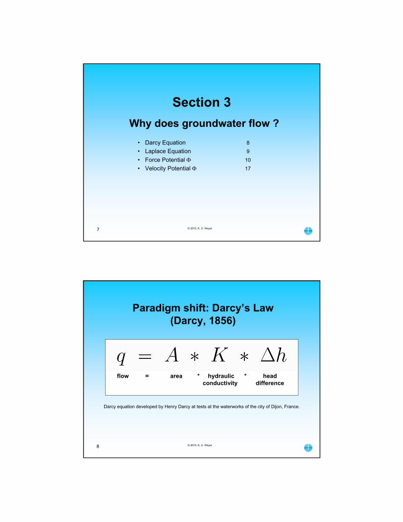
Why does groundwater flow ?
• Darcy Equation 8
• Laplace Equation 9
• Force Potential 10
• Velocity Potential 17
Section 3
© 2010, K. U. Weyer8
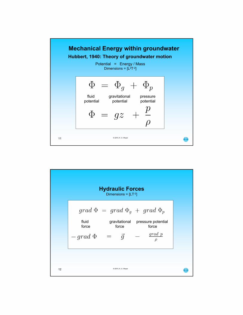
flow = area * hydraulic * head conductivity difference
Darcy equation developed by Henry Darcy at tests at the waterworks of the city of Dijon, France.
Paradigm shift: Darcy’s Law (Darcy, 1856)

Darcy’s equation is linear and not suited to calculate 2-dimensional or 3-dimensional fields. For this purpose the Darcy equation, together with the continuity equation, is transformed into the Laplace equation, which, in the classical hydrodynamics of surface waters (frictionless flow of an ideal fluid), was written in terms of velocity potential
2 = 0 [L2T-1]
This requires that the fluid be incompressible as the velocity potential refers to energy/unit volume. The velocity potential is only a defined mathematical quantity – not a separately measurable physical quantity – whose value at each point is determined solely by the velocity field [Hubbert, 1940].
Slichter,1899, wrote the Laplace equation in terms of pressure p, which was also a physically-inadequate approach using energy/unit volume.
2p = 0 [ML-1T-2]
Hubbert’s great step forward was the introduction of the hydraulic potential, which relates the energy to mass and deals with compressible fluids. Then the Laplace equation can be written in terms of the hydraulic force potential
2 = 0 [L2T-2]
representing physically valid fields. In the following we will shift our attention to the physical meaning of and the related force fields. The physical properties of the fields involved can be measured in nature.
Explanation of Laplace Operator
© 2010, K. U. Weyer9
Transfer of Darcy’s equation into the Laplace equation
Dimensions: L = lengthT = time M = mass
© 2010, K. U. Weyer10
• Forces: gravitational, pressure potential and capillary
Paradigm shift: Force Potential (Hubbert, 1940)
© 2010, K. U. Weyer
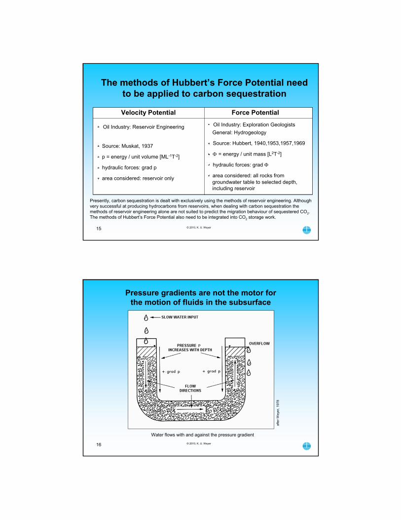
Hubbert, 1940: Theory of groundwater motion
fluid gravitational pressurepotential potential potential
Potential = Energy / MassDimensions = [L2T-2]
11
Mechanical Energy within groundwater
© 2010, K. U. Weyer
Hydraulic ForcesDimensions = [LT-2]
12
fluid gravitational pressure potentialforce force force

© 2010, K. U. Weyer13
after Weyer, 1978
Vectoral addition of hydraulic force directionsThe direction of the total hydraulic force is fundamentally different from the
direction of the pressure potential force
© 2010, K. U. Weyer14
A non-physical approach leading to incorrect flow directions, volume and velocity
volumetric = intrinsic dynamic ● pressureflow vector permeability viscosity gradient
[Muskat, 1937, The Flow of Homogeneous Fluids Through Porous Med[Muskat, 1937, The Flow of Homogeneous Fluids Through Porous Media]ia]
formerly known as “The Bible” of reservoir engineering
Compare with the previous slide: the direction and the magnitude of the pressure vector can be substantially different from that of the hydraulic force ‘– grad ’ leading to erroneous results for direction, volume and velocity of flow.
15
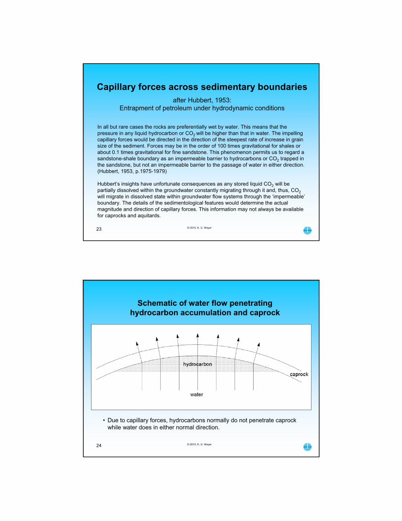
The methods of Hubbert’s Force Potential need to be applied to carbon sequestration
Velocity Potential
Oil Industry: Reservoir Engineering
Source: Muskat, 1937
p = energy / unit volume [ML-1T-2]
hydraulic forces: grad p
area considered: reservoir only
Force Potential
Oil Industry: Exploration Geologists
General: Hydrogeology
Source: Hubbert, 1940,1953,1957,1969
= energy / unit mass [L2T-2]
hydraulic forces: grad
area considered: all rocks from groundwater table to selected depth,including reservoir
Presently, carbon sequestration is dealt with exclusively using the methods of reservoir engineering. Although very successful at producing hydrocarbons from reservoirs, when dealing with carbon sequestration the methods of reservoir engineering alone are not suited to predict the migration behaviour of sequestered CO2. The methods of Hubbert’s Force Potential also need to be integrated into CO2 storage work.
© 2010, K. U. Weyer
© 2010, K. U. Weyer16
afte
r W
eyer
, 197
8
Pressure gradients are not the motor for the motion of fluids in the subsurface
Water flows with and against the pressure gradient

© 2010, K. U. Weyer17
Velocity Potential Muskat, 1937, The Flow of Homogeneous Fluids Through Porous Media,
Equation 3.3(3) = energy / unit volume; dimension [L2T-1]
= k/ (p - gz) Muskat, 1937, integrated the gravity as a vertical body force within the equation for velocity potential. Physical analysis shows that method to be unsuitable for 2D and 3D flow fields in anisotropic and/or heterogeneous media. It also assumed incompressible, frictionless, “ideal fluids” (Hubbert, 1969, p.16). Hence, it cannot be used for general calculations of fluid flow in the subsurface.
Hubbert’s (1940, 1953, 1957, 1969) rigorous treatises consolidated the scientific basis of groundwater hydrology within the general theory of hydrodynamics. (de Vries, 2007, p.1-20.)
18
• Role of fresh water force fields 19• Hydrostatic forces versus hydrodynamic forces 20• Determination of flow directions for all fluids in the
subsurface 21• Capillary forces 22
Why do other fluids flow in the subsurface?
Section 4
© 2010, K. U. Weyer

19
Under natural conditions, the fresh water energy field of hydraulic potentials determines the state
of energy for all fluids in the subsurface
Hubbert, 1953, p.1960:
“The generality of the fluid potential, as here defined, merits attention. The potential is determinable not only in the space occupied by the given fluid, but also at any point capable of being occupied by that fluid. Thus fresh water potentials have values not only in space saturated with fresh water, but also in space occupied by other fluids such as air, salt water, or oil or gas. In each case the potential is the amount of work required to transport unit mass of the fluid to that point from the standard state.”
The derived fresh water force field determines the pressure potential forces for all fluids present, such as air, salt water, oil, gas, or CO2. Hence, proper understanding of fresh water force fields is a necessary foundation for CO2 storage.
© 2010, K. U. Weyer
© 2010, K. U. Weyer
after Hubbert, 1953: Entrapment of Petroleum Under Hydrodynamic Conditions, Fig. 4
20
There is no principle difference between hydrostatic and hydrodynamic forces. Hydrostatic conditions (A) are a special hydrodynamic condition wherein the pressure potential gradient is equal in size to the gravitational force, but pointing in the opposite direction. Hence, the hydraulic forces are equal to 0 and the water does not flow.
Under hydrodynamic conditions (B), the water flows and the fresh water pressure potential gradient is either not pointing in opposition to the gravitational gradient g, or is of different magnitude.
[See Section 8 for more detailed discussions]
Hydraulic forces (grad under hydrostatic and hydrodynamic conditions

© 2010, K. U. Weyer
Hubbert, 1953: Entrapment of Petroleum Under Hydrodynamic Conditions
21
• The pressure potentials of fresh water determine the pressure potentials for all other fluids (oil, gas, CO2, salt water) within the ubiquitous energy field created by fresh groundwater
• The lower densities of oil and gas cause stronger pressure potential forces to maintain, within the freshwater field, the same energy status for the less dense fluids. The pressure potential force of water is divided by the densities for oil and gas.
• Vectoral addition in turn leads to significantly differing flow directions within the same energy field as shown.
• Liquid CO2 has a density similar to that of oil at about 0.85 g/cm3.
• Salt water gradients were not shown in the diagram by Hubbert. Slide 87 in Section 7 shows that ocean-type salt water has almost the same flow direction as fresh water.
[See Section 8 for more detailed discussions]
Determination of flow directions for all fluids in the subsurface
© 2010, K. U. Weyer
Capillary potential and forces in CO2after Hubbert, 1953:
Entrapment of petroleum under hydrodynamic conditions
fluid gravitational pressure capillaryforce force potential force
force
22
fluid gravitational pressure capillarypotential potential potential potential
Capillary forces across sedimentary boundariesafter Hubbert, 1953:
Entrapment of petroleum under hydrodynamic conditions
23 © 2010, K. U. Weyer
In all but rare cases the rocks are preferentially wet by water. This means that the pressure in any liquid hydrocarbon or CO2 will be higher than that in water. The impelling capillary forces would be directed in the direction of the steepest rate of increase in grain size of the sediment. Forces may be in the order of 100 times gravitational for shales or about 0.1 times gravitational for fine sandstone. This phenomenon permits us to regard a sandstone-shale boundary as an impermeable barrier to hydrocarbons or CO2 trapped in the sandstone, but not an impermeable barrier to the passage of water in either direction.(Hubbert, 1953, p.1975-1979)
Hubbert’s insights have unfortunate consequences as any stored liquid CO2 will be partially dissolved within the groundwater constantly migrating through it and, thus, CO2will migrate in dissolved state within groundwater flow systems through the ‘impermeable’boundary. The details of the sedimentological features would determine the actual magnitude and direction of capillary forces. This information may not always be available for caprocks and aquitards.
24
Schematic of water flow penetrating hydrocarbon accumulation and caprock
• Due to capillary forces, hydrocarbons normally do not penetrate caprock while water does in either normal direction.
© 2010, K. U. Weyer
© 2010, K. U. Weyer25
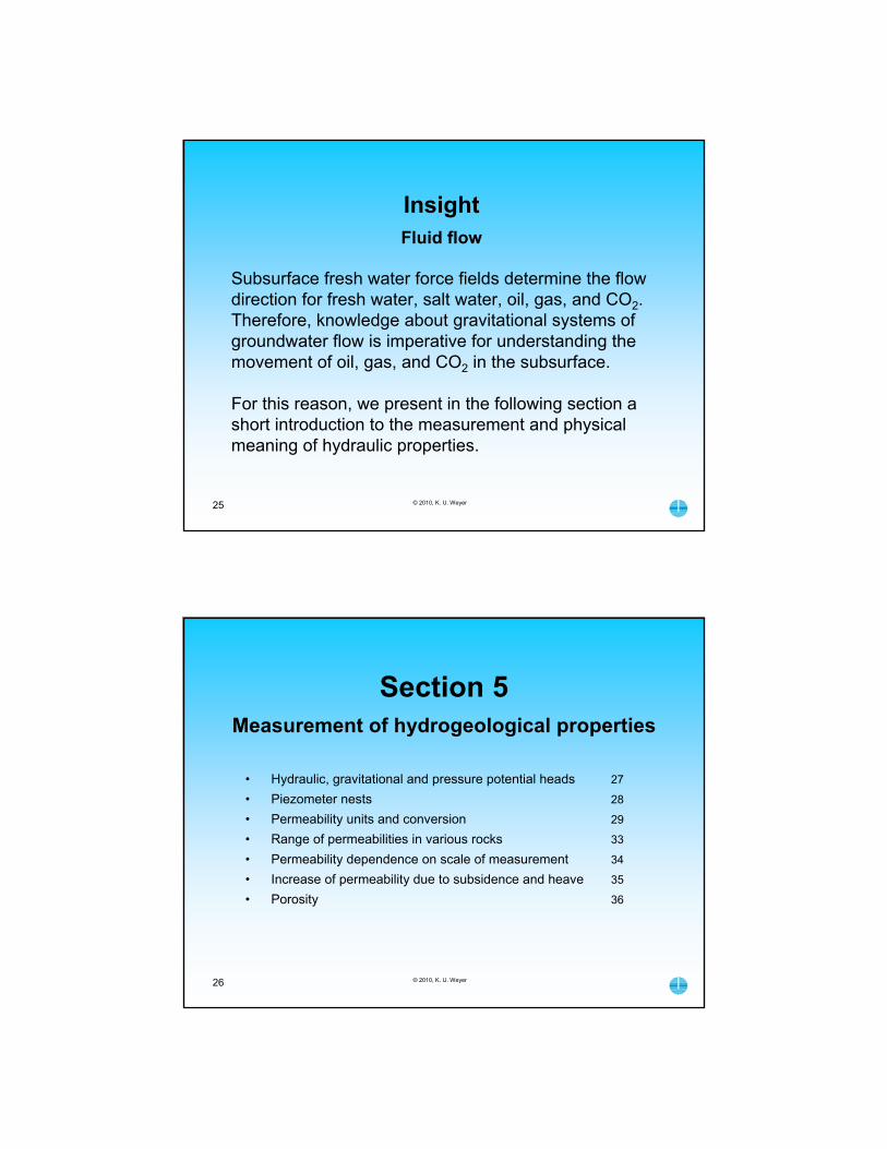
Subsurface fresh water force fields determine the flow direction for fresh water, salt water, oil, gas, and CO2. Therefore, knowledge about gravitational systems of groundwater flow is imperative for understanding the movement of oil, gas, and CO2 in the subsurface.
For this reason, we present in the following section a short introduction to the measurement and physical meaning of hydraulic properties.
InsightFluid flow
© 2010, K. U. Weyer26
Measurement of hydrogeological properties
• Hydraulic, gravitational and pressure potential heads 27
• Piezometer nests 28
• Permeability units and conversion 29
• Range of permeabilities in various rocks 33
• Permeability dependence on scale of measurement 34
• Increase of permeability due to subsidence and heave 35
• Porosity 36
Section 5
© 2010, K. U. Weyer27
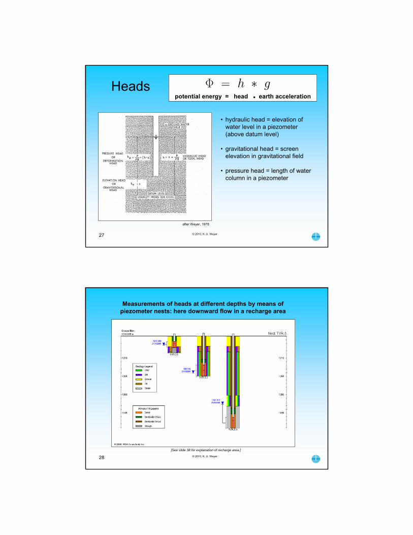
after Weyer, 1978
potential energy = head ● earth acceleration
• hydraulic head = elevation of water level in a piezometer (above datum level)
• gravitational head = screen elevation in gravitational field
• pressure head = length of water column in a piezometer
Heads
© 2010, K. U. Weyer28
Measurements of heads at different depths by means of piezometer nests: here downward flow in a recharge area
[See slide 38 for explanation of recharge area.]
© 2010, K. U. Weyer29
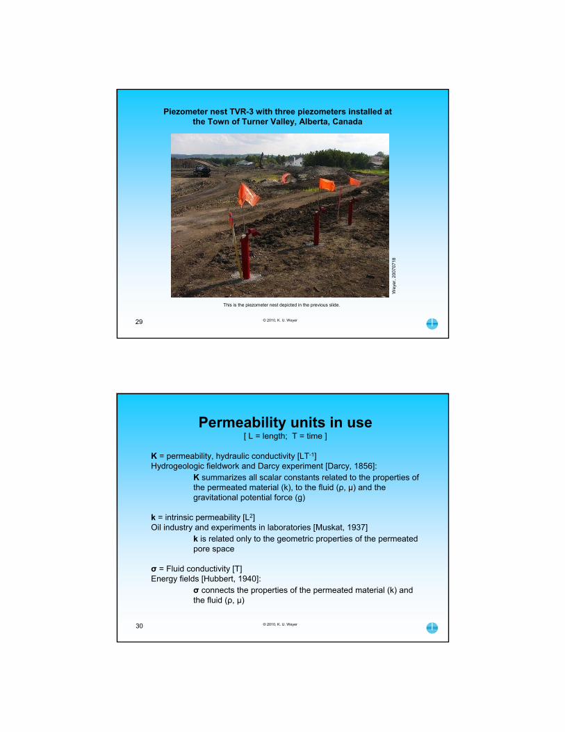
Piezometer nest TVR-3 with three piezometers installed at the Town of Turner Valley, Alberta, Canada
Wey
er, 2
0070
718
This is the piezometer nest depicted in the previous slide.
© 2010, K. U. Weyer30
Permeability units in use[ L = length; T = time ]
K = permeability, hydraulic conductivity [LT-1]Hydrogeologic fieldwork and Darcy experiment [Darcy, 1856]:
K summarizes all scalar constants related to the properties of the permeated material (k), to the fluid (ρ, μ) and the gravitational potential force (g)
k = intrinsic permeability [L2]Oil industry and experiments in laboratories [Muskat, 1937]
k is related only to the geometric properties of the permeated pore space
σ = Fluid conductivity [T] Energy fields [Hubbert, 1940]:
σ connects the properties of the permeated material (k) and the fluid (ρ, μ)
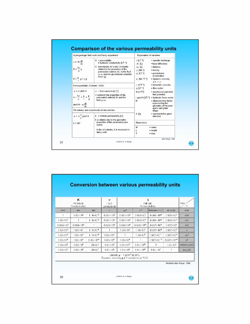
© 2010, K. U. Weyer31after Weyer, 1996
Comparison of the various permeability units
© 2010, K. U. Weyer32
Modified after Weyer, 1996
Conversion between various permeability units

© 2010, K. U. Weyer33
data
take
n fr
om F
reez
e &
Che
rry,
197
9
Range of permeabilities in various rocks
© 2010, K. U. Weyer34
Representation of scale effect on permeability in karstic rocks.
modified from Kiraly, 1975, Figure 19
On a regional scale the actual effective permeabilities may be up to four orders of magnitude higher than those measured in wells and cores. This also applies to many fractured rocks.
© 2010, K. U. Weyer35
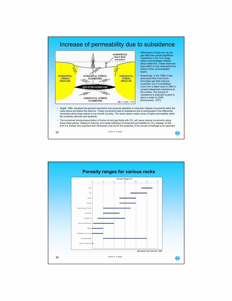
Increase of permeability due to subsidence• Withdrawal of fluids from oil and
gas fields has caused significant subsidence in the 10 m range within unconsolidated material above reservoirs. These reservoirs were within or very close below the bottom of the unconsolidated layers.
• Surprisingly, in the 1960s it was discovered that in the Dutch Groningen gas field reservoir production out of consolidated rocks from a depth close to 3000 m caused widespread subsidence at the surface. The amount of subsidence is expected to grow to about a meter by 2050. [Schoonbeek, 1977].
• Segall, 1989, visualized the general mechanics how pressure depletion in reservoirs initiates movements within the rocks above and below the reservoir. These movements lead to subsidence and to earthquakes if the differential movement along shear planes is not smooth but jerky. The shear planes create zones of higher permeability within the overlying caprocks and aquitards.
• The envisioned strong pressurization of former oil and gas fields with CO2 will cause reverse movements along these sheer planes, leading to heaving, and create pathways of enhanced permeability for CO2 leakage. At this time it is unclear how important that mechanism may be for the prediction of the amount of leakage to be expected.
© 2010, K. U. Weyer36
data taken from Driscoll, 1986
Porosity ranges for various rocks

© 2010, K. U. Weyer37
How does groundwater flow?
• Paradigm Shift Hubbert, 1940: Force Potential 38- Hubbert’s theoretical approximation of groundwater flow between two valleys- Sand model of groundwater flow and 2D-vertical mathematical model [1]
• Counterplay of forces 50
• Paradigm Shift Tóth, 1962: Groundwater Flow Systems 56- Field example: Turner Valley, Alberta- Mathematical model [2] by Tóth [1962]- Mathematical models [3] by Freeze and Witherspoon [1967]- Continuity of flow between aquitard and aquifer- Field example France: How to see groundwater flow systems penetrate aquitards- Erroneous assumptions about regional groundwater flow- Field example and 2D-vertical mathematical model [4]: Brake landfill in Germany
• Silt [10-8 m/s, 1 mD] as an efficient hydraulic window 75- Field example and 3D-mathematical model [5]: Düsseldorf/Hilden, Germany
Section 6
© 2010, K. U. Weyer38
afte
r H
ubbe
rt, 1
940
The figure depicts Hubbert’s schematic diagram of gravitational groundwater flow between two valleys. The terminology ‘recharge area’ and ‘discharge area’ was introduced by Tóth, 1962:Recharge area = area of groundwater table where water moves into the groundwater bodyDischarge area = area of groundwater table where water moves out of the groundwater body
Paradigm Shift Hubbert, 1940: Force Potential
© 2010, K. U. Weyer39
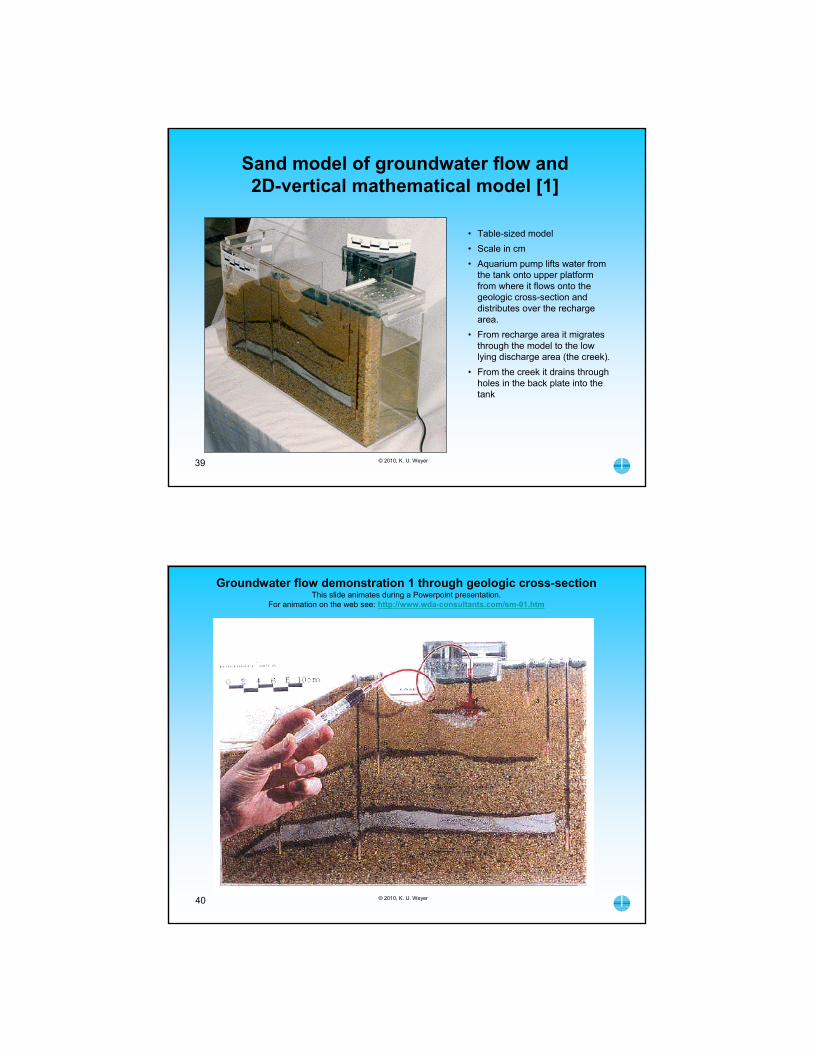
Sand model of groundwater flow and 2D-vertical mathematical model [1]
• Table-sized model
• Scale in cm
• Aquarium pump lifts water from the tank onto upper platform from where it flows onto the geologic cross-section and distributes over the recharge area.
• From recharge area it migrates through the model to the low lying discharge area (the creek).
• From the creek it drains through holes in the back plate into the tank
© 2010, K. U. Weyer40
Groundwater flow demonstration 1 through geologic cross-sectionThis slide animates during a Powerpoint presentation.
For animation on the web see: http://www.wda-consultants.com/sm-01.htm

© 2010, K. U. Weyer41
Groundwater flow demonstration 2 through geologic cross-sectionThis slide animates during a Powerpoint presentation.
For animation on the web see: http://www.wda-consultants.com/sm-02.htm
© 2010, K. U. Weyer42
Groundwater flow demonstration 3 through geologic cross-sectionThis slide animates during a Powerpoint presentation.
For animation on the web see: http://www.wda-consultants.com/sm-03.htm

© 2010, K. U. Weyer43
Weyer, 1996
The term ‘artesian’ is derived from the area of Artois in France. There, artesian wells [water level above surface] had been dug and their flow admired since the middle ages.
Truly artesian conditions indicate discharge areas with upward-directed groundwater flow. The definition of artesian by Jacob [1940], water level in well above top of aquifer, confined aquifer] is hydraulically meaningless and should be avoided.
Artesian wells
© 2010, K. U. Weyer44
2D-vertical steady-state model calculation for the determination of flow directions in cross-sections
[here: sand model]
• Precursors of this method were originally applied by Freeze and Witherspoon, 1966, 1967 for theoretical understanding of the context between topography, geology, and groundwater flow systems.
• Weyer, 1996, applied the method to real field situations and showed how the estimation of permeability contrasts (relative permeabilities) and equating the groundwater table to the topography, returned, in larger-scale cross-sections of several kilometers in length, surprisingly realistic results for equipotential and flow lines in the first model run. This eliminated the field determination of permeabilities and the calibration of models for the determination of flow directions within cross-sections. This approach to modeling has proved ideal for the formation of concepts and the design of monitoring systems.
• The method has now been adopted for the investigation of carbon sequestration sites.

45
Cross-section of sand model as base for mathematical model [1]Shown are the recharge area, discharge area, ‘unconfined’ aquifer, aquitard,
‘confined’ aquifer, water wells and an artesian well in the discharge area
© 2010, K. U. Weyer
© 2010, K. U. Weyer
Mathematical model [1]: estimation of permeability contrasts [A] and design of finite element grid [B]
46
A
B
after Weyer, 1996
• The estimation of permeabilities was roughly based on grain sizes.
• The model grid consists of approximately 1400 elements
• Artesian flow through the artesian well was not part of the groundwater simulation.
© 2010, K. U. Weyer
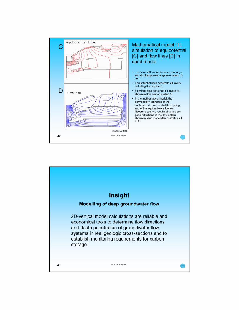
Mathematical model [1]:simulation of equipotential [C] and flow lines [D] in sand model
47
C
D
after Weyer, 1996
47
• The head difference between recharge and discharge area is approximately 10 cm.
• Equipotential lines penetrate all layers including the ‘aquitard’.
• Flowlines also penetrate all layers as shown in flow demonstration 3.
• In the mathematical model, the permeability estimates of the contaminants area and of the dipping end of the aquitard were too low. Nevertheless, the results obtained are good reflections of the flow pattern shown in sand model demonstrations 1 to 3.
© 2010, K. U. Weyer48
2D-vertical model calculations are reliable and economical tools to determine flow directions and depth penetration of groundwater flow systems in real geologic cross-sections and to establish monitoring requirements for carbon storage.
InsightModelling of deep groundwater flow

© 2010, K. U. Weyer49
2D-vertical model calculations for the determination of flow directions in real geologic cross-sections
2D-vertical steady-state calculations of groundwater flow in deep reaching cross-sections are a reliable way to determine penetration depth and flow directions of groundwater flow systems as shown in a research project by Weyer, 1996. Permeabilities are entered as estimated permeability contrasts, thus eliminating the field determination of permeabilities and porosities.
The contrast estimations are very tolerant in such that fairly wide contrast variations between higher and lower permeable layers return rather stable flow patterns and directions. The regional scale of the geologic cross-sections allows the assumption of a groundwater table as a boundary condition close to the topographic surface thus eliminating any calibration runs. The results of the models Brake and Münchehagen, shown later in this primer, are each based on only one model run.
© 2010, K. U. Weyer50
Counterplay of hydraulic forces
• Equipotential lines along a schematic flow line
• Changes of heads along a schematic flow line
• How is the mechanical pressure potential generated in nature?
• Vector additions along a flow line

© 2010, K. U. Weyer51
after Weyer, 1978
Schematics of equipotential lines and flow line(Not to scale)
Hydrodynamic conditions
• Hydraulic heads are the blue lines which decrease in value from the recharge area (hill) to the discharge area (valley).
• The gravitational heads are the horizontal elevation lines
• The pressure potential heads are dotted in red. In the recharge area they are further apart (lesser gradient) than in the discharge area (higher gradient).
• The pressure and the pressure potential gradient are notdetermined by the column of water above the point of consideration.
© 2010, K. U. Weyer52
after Weyer, 1978
Schematics of changes of heads along a flow line(Not to scale)
Hydrodynamic conditions
• The total head (blue line in [B]) diminishes consistently along the flow line from the recharge to the discharge area (see positions 1 to 5)
• The gravitational head (grey line in [B]) is reduced in areas of downward flow (recharge area) and increases in areas of upward flow (discharge area) (see positions 1 to 5).
• The pressure potential head (red line in [B]) increases in areas of downward flow and decreases in areas of upwards flow (see positions 1 to 5).
• Exception: In conditions of Buoyancy Reversal the pressure potential head decreases with forced downward flow through low permeable layers [see section 9 on ‘Buoyancy Reversal’].
[A]
[B]
© 2010, K. U. Weyer53
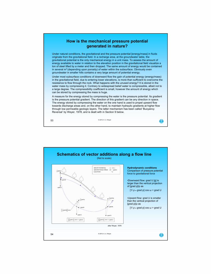
How is the mechanical pressure potential generated in nature?
Under natural conditions, the gravitational and the pressure potential [energy/mass] in fluids originate from the gravitational field. In a recharge area, at the groundwater table, thegravitational potential is the only mechanical energy in a unit mass. To assess the amount of energy available to water in relation to the elevation position in the gravitational field visualize a ton of steel lifted by a meter and then dropped. The same amount of energy would be contained in several m3 (depending upon porosity) of water within the subsurface. Obviously even groundwater in smaller hills contains a very large amount of potential energy.
Under most subsurface conditions of downward flow the gain of potential energy (energy/mass) in the gravitational field, due to entering lower elevations, is more than sufficient to overcome the resistance to flow through the rock. What happens with the unused energy? It is stored in the water mass by compressing it. Contrary to widespread belief water is compressible, albeit not to a large degree. The compressibility coefficient is small, however the amount of energy which can be stored by compressing the mass is huge.
A measure for the energy stored by compressing the water is the pressure potential. Its gradient is the pressure potential gradient. The direction of this gradient can be any direction in space. The energy stored by compressing the water on the one hand is used to propel upward flow towards discharge areas and, on the other hand, to maintain hydraulic gradients at higher flow through low permeable geologic layers. The latter mechanism has been called ‘Buoyancy Reversal’ by Weyer, 1978, and is dealt with in Section 9 below.
© 2010, K. U. Weyer54
after Weyer, 1978
Schematics of vector additions along a flow line(Not to scale)
Hydrodynamic conditionsComparison of pressure potential force to gravitational force
•Downward flow: grad U [g] is larger than the vertical projection of [grad p]/ρ as
[1/ ρ ● grad p] cos ω < grad U
•Upward flow: grad U is smaller than the vertical projection of [grad p]/ρ as
[1/ ρ ● grad p] cos ω > grad U
© 2010, K. U. Weyer55
What about the state of fluid dynamics of surface water?
Giovanni Gallavotti, 2002. Foundations of Fluid DynamicsGiovanni Gallavotti is a mathematical physicist working at the University of “La Sapienza”, Rome.
P. VII: “The first great surprise was to realize that the mathematical theory of fluids is in an even more primitive state than I was aware of. … One should not forget that the fluid equations do not have a fundamental nature, i.e. they are ultimately phenomenological equations and for this reason one ‘cannot ask too much from them’….”
P. VIII: “The second part of the book is dedicated to the qualitative and phenomelogical theory of the incompressible Navier-Stokes equation: the lack of existence and uniqueness theorems (in three space dimensions) had little or no practical consequences on research. Fearless engineers write gigantic codes that are supposed to produce solutions to the equations: They do not care the least (when they are conscious of the problem, which seldom seems to be the case) that what they study are not the Navier-Stokes equations, but just the informatic code they produced. No one is, to date, capable of writing an algorithm, that in an a priori known time and within a prefixed approximation, will produce the calculation of any property of the equations solution following an initial datum and forces which are not ‘very small’ or ‘very special’. Statements to the contrary are not rare, and they may appear even in the news: but they are wrong”.
Comment: It appears that subsurface fluid dynamics may have progressed further than that of surface water due to the work of Hubbert and possibly due to less chaotic conditions. The Navier-Stokes equations are not suited as a base for groundwater dynamics due to their assumption that water is incompressible.
© 2010, K. U. Weyer56
The theory of Groundwater Flow Systems originated in the Alberta Research Council (of the time) in response to cable tool drilling data from oil wells in the Turner Valley oilfield SW of Calgary, Alberta. In the 1920s drilling was done without fluid circulation. Drilling on hills encountered decreasing water levels with depth once the groundwater table had been penetrated. In valleys the water levels rose with drilling depth and turned artesian. At the shoulder of valleys the water level did not change. This behaviour was finally explained by applying Hubbert’s [1940] Force Potential, which up to this time had been widely considered an absurd opinion within hydrogeology.
In an attempt to explain additional hydrogeological field evidence, electrical Teledeltos paper models of geological cross-sections and simplified analytical calculations led to the formulation of the principals of Groundwater Flow Systems [Tóth, 1962].
Freeze and Witherspoon [1966, 1967] determined the effect of topography and geologic structures of differing permeabilities upon groundwater flow patterns by simulating groundwater flow systems in 2D-vertical geologic cross-sections using early numerical computer models.
Paradigm Shift: Groundwater Flow Systems (Tóth, 1962)
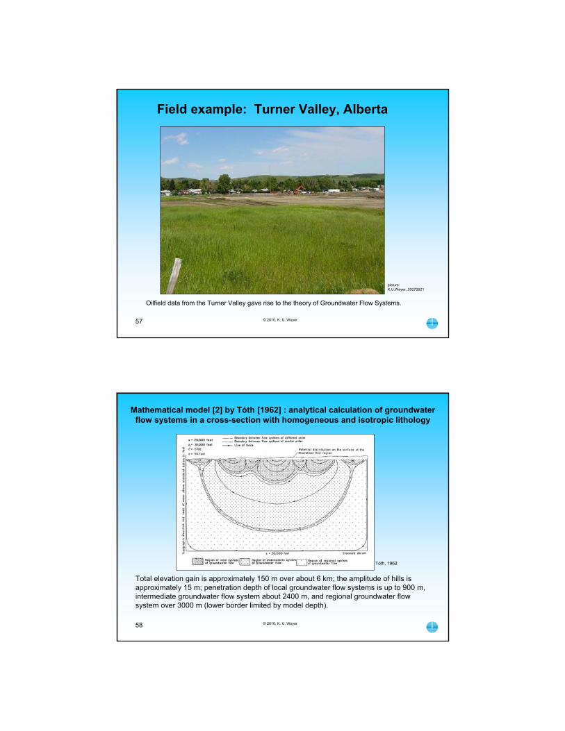
© 2010, K. U. Weyer57
Oilfield data from the Turner Valley gave rise to the theory of Groundwater Flow Systems.
Field example: Turner Valley, Alberta
picture:K.U.Weyer, 20070621
Total elevation gain is approximately 150 m over about 6 km; the amplitude of hills is approximately 15 m; penetration depth of local groundwater flow systems is up to 900 m, intermediate groundwater flow system about 2400 m, and regional groundwater flow system over 3000 m (lower border limited by model depth).
© 2010, K. U. Weyer58
Tóth, 1962
Mathematical model [2] by Tóth [1962] : analytical calculation of groundwater flow systems in a cross-section with homogeneous and isotropic lithology

© 2010, K. U. Weyer59
Mathematical models [3] by Freeze and Witherspoon [1967]: effect of topography [1] and buried higher-permeable layer [2] upon groundwater
flow pattern and location of recharge and discharge areas.
Permeability contrasts, dimensionless distance and depth [S] were applied. Geologic layers are homogeneous and isotropic. In figure [2], twice as much water flows within the aquitard (down and up) as within the aquifer (lateral).
[1]
[2]
after Freeze and Witherspoon, 1967
© 2010, K. U. Weyer60
Mathematical models [3] by Freeze and Witherspoon [1967]: Effect of buried higher-permeable layer [1,2] upon groundwater flow pattern and
location of recharge and discharge areas
[1]
[2]
Permeability contrasts, dimensionless distance and depth [S] were applied. Geologic layers are homogeneous and isotropic. In figure [2] (flowlines added), twice as much water flows within the aquitard (down and up) as within the aquifer (lateral).
after Freeze and Witherspoon, 1967

© 2010, K. U. Weyer61
Continuity of flow between aquitard and aquifer(under natural hydraulic conditions)
afte
r W
eyer
, 199
6
© 2010, K. U. Weyer62
Schematic diagram of groundwater flow with aquitard over buried aquifer
Twice as much groundwater flows through the aquitard (vertically down and up) as through the aquifer (only once laterally). The head distribution in the aquifer is a replica of the topography. In recharge areas the potential in the aquifer is lower than that at the groundwater table, in discharge areas the potential in the buried aquifer is higher than that at the groundwater table.
62
after Weyer, 1996
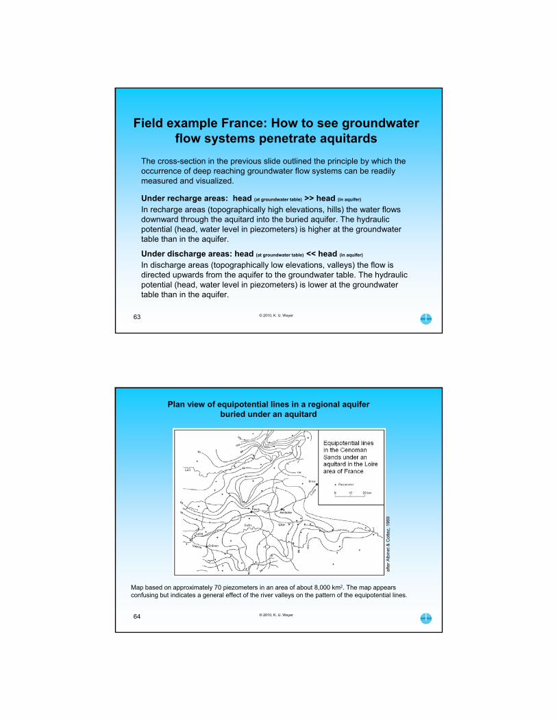
© 2010, K. U. Weyer63
Field example France: How to see groundwater flow systems penetrate aquitards
The cross-section in the previous slide outlined the principle by which the occurrence of deep reaching groundwater flow systems can be readily measured and visualized.
Under recharge areas: head (at groundwater table) >> head (in aquifer)
In recharge areas (topographically high elevations, hills) the water flows downward through the aquitard into the buried aquifer. The hydraulic potential (head, water level in piezometers) is higher at the groundwater table than in the aquifer.
Under discharge areas: head (at groundwater table) << head (in aquifer)
In discharge areas (topographically low elevations, valleys) the flow is directed upwards from the aquifer to the groundwater table. The hydraulic potential (head, water level in piezometers) is lower at the groundwater table than in the aquifer.
© 2010, K. U. Weyer64
afte
r A
lbin
et &
Cot
tez,
196
9
Plan view of equipotential lines in a regional aquifer buried under an aquitard
Map based on approximately 70 piezometers in an area of about 8,000 km2. The map appears confusing but indicates a general effect of the river valleys on the pattern of the equipotential lines.

Recharge and discharge areas are outlined by differences in hydraulic heads (water levels) in piezometers. Subtracting head values in the aquifer from those at the groundwater table. Negative values indicate areas of upward flow through aquitard and discharge. They are hatched and shown in yellow.
© 2010, K. U. Weyer65
afte
r A
lbin
et &
Cot
tez,
196
9
Plan view of groundwater flow systems penetrating an aquitard
© 2010, K. U. Weyer
Hubbert, 1953: Entrapment of Petroleum Under Hydrodynamic Conditions
66
Erroneous assumptions about regional groundwater flow 1
Hubbert restricted flow to the aquifer. Knowledge about groundwater flow systems penetrating aquitards only became available more than a decade later (Freeze and Witherspoon, 1966, 1967).
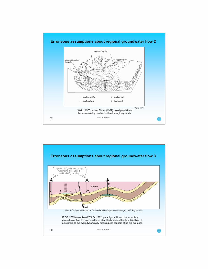
© 2010, K. U. Weyer67
Waltz, 1973
Waltz, 1973 missed Tóth’s (1962) paradigm shift and the associated groundwater flow through aquitards
Erroneous assumptions about regional groundwater flow 2
© 2010, K. U. Weyer
After IPCC Special Report on Carbon Dioxide Capture and Storage, 2005, Figure 5.25
68
IPCC, 2005 also missed Tóth’s (1962) paradigm shift, and the associated groundwater flow through aquitards, about forty years after its publication. It also refers to the hydrodynamically-meaningless concept of up-dip migration.
Erroneous assumptions about regional groundwater flow 3
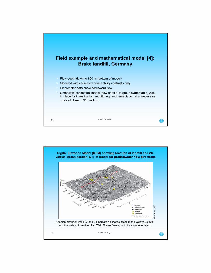
© 2010, K. U. Weyer69
Field example and mathematical model [4]: Brake landfill, Germany
• Flow depth down to 800 m (bottom of model)
• Modeled with estimated permeability contrasts only
• Piezometer data show downward flow
• Unrealistic conceptual model (flow parallel to groundwater table) was in place for investigation, monitoring, and remediation at unnecessary costs of close to $10 million.
© 2010, K. U. Weyer70
afte
r W
eyer
, 199
6Digital Elevation Model (DEM) showing location of landfill and 2D-
vertical cross-section W-E of model for groundwater flow directions
Artesian (flowing) wells 22 and 23 indicate discharge areas in the valleys Jölletaland the valley of the river Aa. Well 22 was flowing out of a claystone layer.

© 2010, K. U. Weyer71
afte
r W
eyer
, 199
6
Erroneous conceptual model of groundwater flow in place for investigation and remediation at Brake landfill
The weathered clay layer over Liassic claystone misled investigators into believing that the shallow groundwater could not to the claystone layer as the weathered clay was considered an aquitard.
© 2010, K. U. Weyer72
Cross-section through Brake landfill showing recharge area with downward flow
afte
r W
eyer
, 199
6
Because of the erroneous concept of groundwater flow, the investigators interpreted the lower water level in the deeper piezometers as proof that the two aquifers were not connected due to the weathered clay layer and consequently overlooked that groundwater was flowing downward from the shallow aquifer into the claystone.
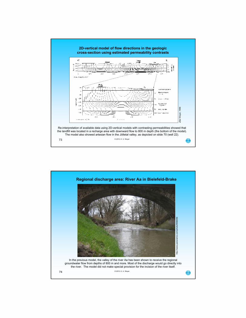
© 2010, K. U. Weyer73
afte
r W
eyer
, 199
6
2D-vertical model of flow directions in the geologic cross-section using estimated permeability contrasts
Re-interpretation of available data using 2D-vertical models with contrasting permeabilities showed that the landfill was located in a recharge area with downward flow to 800 m depth (the bottom of the model).
The model also showed artesian flow in the Jölletal valley, as depicted on slide 70 (well 22).
© 2010, K. U. Weyer74
Regional discharge area: River Aa in Bielefeld-Brakeht
tp://
ww
w.p
anor
amio
.com
/pho
to/8
5684
56
In the previous model, the valley of the river Aa has been shown to receive the regional groundwater flow from depths of 800 m and more. Most of the discharge would go directly into
the river. The model did not make special provision for the incision of the river itself.

© 2010, K. U. Weyer75
Field example and mathematical model [5]:
• Long term field investigations of groundwater contamination by chlorinated hydrocarbons near Düsseldorf, Germany showed the groundwater to flow through a silt window into the underlying dolomite with heads 15 m deeper than in the quaternary layers (regional drawdown caused by mine dewatering)
• A regional 3D-groundwater flow model with about a million elements, based on actual field permeabilities, showed the main downward-directed flow penetrating a hydraulic window of silt within a clay layer
• Annual travel distances are shown by dots calculated by particle tracking of flow lines
• Permeabilities determined for clay (~0.1 mD) and the silt window (5 mD) are similar to typical values for caprock (0.1 mD) and reservoirs (10 mD). The result of the model also established significant flow through the clay layer.
Silt [10-8 m/s, 1mD] as an efficient hydraulic window
© 2010, K. U. Weyer76
Configuration of 3D-finite-element flow modelaf
ter
Wey
er a
nd M
ols
on, 2
004
Oblique view of the 3D flow model Düsseldorf/Hilden with cross-section A-A’. Geology of cross-section A-A’ is shown on the next slide. Equipotential lines are shown in
figure [E] of slide 78 and flow lines in [F] of the same slide.

© 2010, K. U. Weyer77
afte
r W
eyer
and
Mo
lson
, 200
4
Geologic cross-section A-A’ with silt window
Dark blue = quaternary and dolomite Orange = clay layer Yellow-orange = silt window
Silt window: 5 x 10⁻⁸ m/s Silt window: ~5 mD Clay layer: 1 x 10⁻⁹ m/s Clay layer: ~0.1 mD
The hydraulic conductivities (intrinsic permeabilities) of the silt window and clay layer are similar to values used by Gasda et al. (2008) for caprock (0.1 mD) and for reservoirs (10 mD).
© 2010, K. U. Weyer78
after Weyer and Molson, 2004
Equipotential lines and flow lines in cross-section A-A’ for calibrated model
[E]: equipotential lines in cross-section
[F]: flow lines in cross-section
• The flow line pattern emphasizes the hydraulic role of the silt window
• Flow also penetrates the clay layer,albeit in smaller amounts (two flow linesupstream of the silt window). Higher gradients, as associated with CO2
storage, would increased the flowthrough the clay layers significantly.
• Annual flow distance (distance between dots) calculated by particletracking
• For geology and permeability see slide 77
• In this model, the permeabilities for theclay layer (~0.1 mD) and the silt window(~5 mD) are similar to typical valuesused by Gasda et al. (2008) for caprock(0.1 mD) and reservoirs (10 mD).
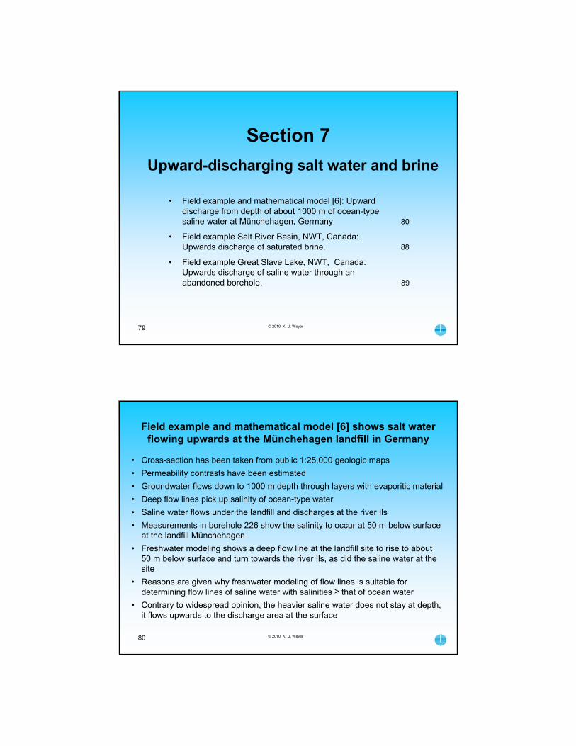
© 2010, K. U. Weyer79
• Field example and mathematical model [6]: Upward discharge from depth of about 1000 m of ocean-type saline water at Münchehagen, Germany 80
• Field example Salt River Basin, NWT, Canada: Upwards discharge of saturated brine. 88
• Field example Great Slave Lake, NWT, Canada: Upwards discharge of saline water through an abandoned borehole. 89
Upward-discharging salt water and brine
Section 7
© 2010, K. U. Weyer80
Field example and mathematical model [6] shows salt water flowing upwards at the Münchehagen landfill in Germany
• Cross-section has been taken from public 1:25,000 geologic maps
• Permeability contrasts have been estimated
• Groundwater flows down to 1000 m depth through layers with evaporitic material
• Deep flow lines pick up salinity of ocean-type water
• Saline water flows under the landfill and discharges at the river Ils
• Measurements in borehole 226 show the salinity to occur at 50 m below surface at the landfill Münchehagen
• Freshwater modeling shows a deep flow line at the landfill site to rise to about 50 m below surface and turn towards the river Ils, as did the saline water at the site
• Reasons are given why freshwater modeling of flow lines is suitable for determining flow lines of saline water with salinities ≥ that of ocean water
• Contrary to widespread opinion, the heavier saline water does not stay at depth, it flows upwards to the discharge area at the surface
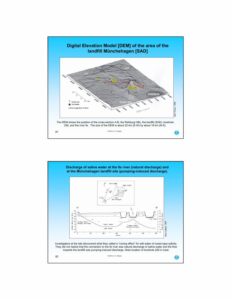
© 2010, K. U. Weyer81
afte
r W
eyer
, 199
6
Digital Elevation Model [DEM] of the area of the landfill Münchehagen [SAD]
The DEM shows the position of the cross-section A-B, the Rehburg Hills, the landfill (SAD), borehole 226, and the river Ils. The size of the DEM is about 22 km (E-W) by about 18 km (N-S).
© 2010, K. U. Weyer82
afte
r Lü
deke
, 198
7Discharge of saline water at the Ils river (natural discharge) and at the Münchehagen landfill site (pumping-induced discharge).
Investigators at the site discovered what they called a “coning effect” for salt water of ocean-type salinity. They did not realize that the connection to the Ils river was natural discharge of saline water and the flow
towards the landfill was pumping-induced discharge. Note location of borehole 226 in inset.

© 2010, K. U. Weyer83
afte
r W
eyer
, 199
6
Geologic cross-section taken from 1:25,000 geologic maps. Calculated groundwater flow directions were based on the groundwater table (following topography) and estimated permeability contrasts.
2D-vertical model of groundwater flow directions in cross-section A-B in the Münchehagen landfill area
© 2010, K. U. Weyer84
Geology and estimation of permeability contrasts for mathematical model of groundwater flow directions in geologic cross-section A-B
Marl with evaporitic components in the MündenerMergel is the source of salinity in the deep flow lines
after Weyer, 1996
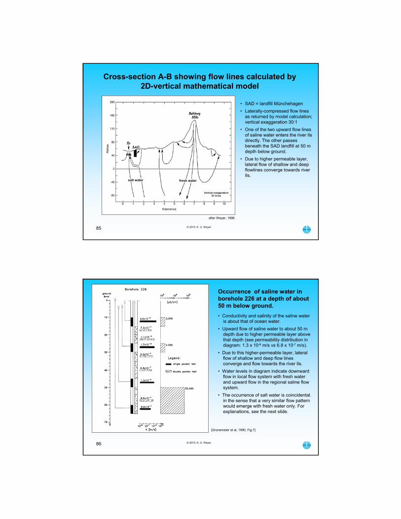
© 2010, K. U. Weyer85
after Weyer, 1996
Cross-section A-B showing flow lines calculated by 2D-vertical mathematical model
• SAD = landfill Münchehagen
• Laterally-compressed flow lines as returned by model calculation; vertical exaggeration 30:1
• One of the two upward flow lines of saline water enters the river Ils directly. The other passes beneath the SAD landfill at 50 m depth below ground.
• Due to higher permeable layer, lateral flow of shallow and deep flowlines converge towards river Ils.
salt water fresh water
© 2010, K. U. Weyer86
[Gronemeier et al, 1990, Fig.7]
Occurrence of saline water in borehole 226 at a depth of about 50 m below ground.
• Conductivity and salinity of the saline water is about that of ocean water.
• Upward flow of saline water to about 50 mdepth due to higher permeable layer abovethat depth (see permeability distribution indiagram: 1.3 x 10⁻⁶ m/s vs 6.8 x 10⁻⁷ m/s).
• Due to this higher-permeable layer, lateralflow of shallow and deep flow linesconverge and flow towards the river Ils.
• Water levels in diagram indicate downwardflow in local flow system with fresh waterand upward flow in the regional saline flowsystem.
• The occurrence of salt water is coincidental.in the sense that a very similar flow patternwould emerge with fresh water only. Forexplanations, see the next slide.

© 2010, K. U. Weyer87
after Weyer, 1996
Why is fresh water modeling suited to determine the flow lines of saline seawater?
• Freshwater determines the field of the potential in the subsurface (see slide 19).
• With a density of 1.03 g/cm3, the vectoral pressure potential force [(grad p)/s] for this ocean-type saline water is very similar in magnitude to that of fresh groundwater with a density of 1.00 g/cm3 and has the same direction.
• Thus, the flow directions are very similar for ocean-type saline groundwater and fresh groundwater.
• This has been verified by the occurrence of saline water at a depth of about 50 m below ground in borehole 226 and in the model results (see slide 85).
© 2010, K. U. Weyer88
Upward discharge of saturated brine near Salt River, NWT, Canada
• Saturated [~350 g/l; density ~1.3 g/cm3] brine dischargingupwards beside a creek
• Salt deposit is caused byprecipitation of salt not byevaporation of brine.
picture: K.U.Weyer, 1977
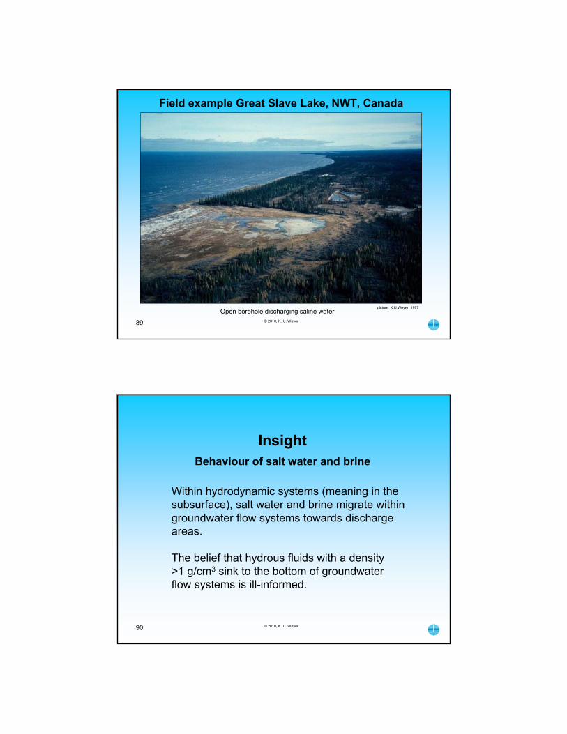
© 2010, K. U. Weyer89
Field example Great Slave Lake, NWT, Canada
Open borehole discharging saline waterpicture: K.U.Weyer, 1977
© 2010, K. U. Weyer90
Within hydrodynamic systems (meaning in the subsurface), salt water and brine migrate within groundwater flow systems towards discharge areas.
The belief that hydrous fluids with a density >1 g/cm3 sink to the bottom of groundwater flow systems is ill-informed.
InsightBehaviour of salt water and brine
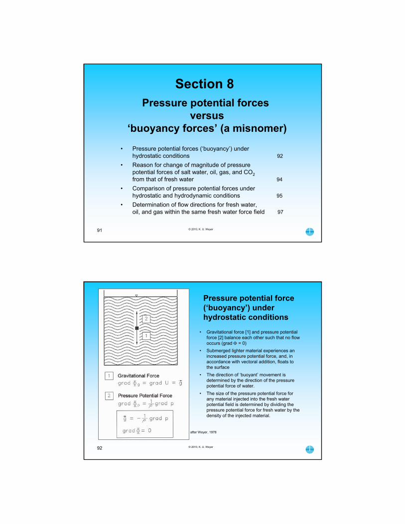
© 2010, K. U. Weyer91
Section 8Pressure potential forces
versus‘buoyancy forces’ (a misnomer)
• Pressure potential forces (‘buoyancy’) under hydrostatic conditions 92
• Reason for change of magnitude of pressure potential forces of salt water, oil, gas, and CO2from that of fresh water 94
• Comparison of pressure potential forces under hydrostatic and hydrodynamic conditions 95
• Determination of flow directions for fresh water, oil, and gas within the same fresh water force field 97
© 2010, K. U. Weyer92
Pressure potential force (‘buoyancy’) under hydrostatic conditions
after Weyer, 1978
• Gravitational force [1] and pressure potential force [2] balance each other such that no flow occurs (grad = 0)
• Submerged lighter material experiences an increased pressure potential force, and, in accordance with vectoral addition, floats to the surface
• The direction of ‘buoyant’ movement is determined by the direction of the pressure potential force of water.
• The size of the pressure potential force for any material injected into the fresh water potential field is determined by dividing the pressure potential force for fresh water by the density of the injected material.
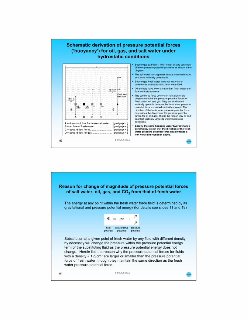
© 2010, K. U. Weyer93
Schematic derivation of pressure potential forces (‘buoyancy’) for oil, gas, and salt water under
hydrostatic conditions
• Submerged salt water, fresh water, oil and gas show different pressure potential gradients as shown in the diagram
• The salt water has a greater density than fresh water and sinks vertically downwards
• Submerged fresh water does not move up or downwards in a hydrostatic fresh water field
• Oil and gas have lower density than fresh water and float vertically upwards
• The combined force vectors on right side of the diagram combine the pressure potential forces of fresh water, oil, and gas. They are all directed vertically upwards because the fresh water pressure potential force is directed vertically upwards. The direction of the fresh water pressure potential force determines the direction of the pressure potential forces for oil and gas. That is the reason why oil and gas float vertically upwards under hydrostatic conditions.
• Exactly the same happens under hydrodynamic conditions, except that the direction of the fresh water pressure potential force usually takes a non-vertical direction in space.
© 2010, K. U. Weyer94
fluid gravitational pressurepotential potential potential
Substitution at a given point of fresh water by any fluid with different density by necessity will change the pressure within the pressure potential energy term of the substituting fluid as the pressure potential energy does not change. Herein lies the reason why the pressure potential forces for fluids with a density 1 g/cm3 are larger or smaller than the pressure potential force of fresh water, though they maintain the same direction as the fresh water pressure potential force.
Reason for change of magnitude of pressure potential forces of salt water, oil, gas, and CO2 from that of fresh water
The energy at any point within the fresh water force field is determined by its gravitational and pressure potential energy (for details see slides 11 and 19)

© 2010, K. U. Weyer95
Comparison of the direction of pressure potential forces under hydrostatic and hydrodynamic conditions
• The hydrostatic part of the diagram shows the pressure potential vectors to be directed vertically-upwards while the hydrodynamic part of the diagram shows a non-vertical direction of pressure potential vectors for all fluids: fresh water, salt water, oil, and gas.
• The direction of any so-called ‘buoyancy force’is determined by the direction of the pressure potential force of fresh water which, under hydrodynamic conditions, may point in any direction in space.
• Division of the water pressure potential force by the density of the ‘buoyant’ fluid determines the size of its pressure potential force.
• The flow direction of the ‘buoyant’ fluid is determined by vectoral addition of the ‘buoyant’ pressure potential force and the gravitational force as shown in the next slide.
© 2010, K. U. Weyer
after Hubbert, 1953: Entrapment of Petroleum Under Hydrodynamic Conditions, Fig.4
96
Hydraulic forces (grad under hydrostatic and hydrodynamic conditions
There is no principle difference between hydrostatic and hydrodynamic forces. Hydrostatic conditions (A) are a special hydrodynamic condition wherein the pressure potential gradient is equal in size to the gravitational force, but pointing in the opposite direction. Hence, the hydraulic forces are equal to 0 and the water does not flow.
Under hydrodynamic conditions (B), the water flows and the fresh water pressure potential gradient is either not pointing in opposition to the gravitational gradient g, or is of different magnitude.[See Section 4 for initial discussions]
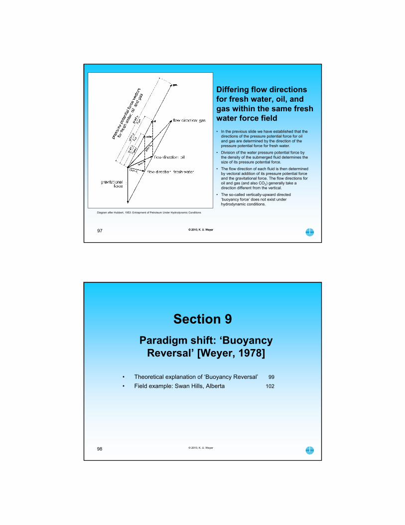
© 2010, K. U. Weyer97 © 2010, K. U. Weyer
Diagram after Hubbert, 1953: Entrapment of Petroleum Under Hydrodynamic Conditions
Differing flow directions for fresh water, oil, and gas within the same fresh water force field
• In the previous slide we have established that the directions of the pressure potential force for oil and gas are determined by the direction of the pressure potential force for fresh water.
• Division of the water pressure potential force by the density of the submerged fluid determines the size of its pressure potential force.
• The flow direction of each fluid is then determined by vectoral addition of its pressure potential force and the gravitational force. The flow directions for oil and gas (and also CO2) generally take a direction different from the vertical.
• The so-called vertically-upward directed ‘buoyancy force’ does not exist under hydrodynamic conditions.
© 2010, K. U. Weyer98
Section 9
Paradigm shift: ‘BuoyancyReversal’ [Weyer, 1978]
• Theoretical explanation of ‘Buoyancy Reversal’ 99
• Field example: Swan Hills, Alberta 102

© 2010, K. U. Weyer99
‘Buoyancy Reversal’
If under conditions of strong downward-directed flow the energy gain within the gravitational field by flow into lower elevations is insufficient to maintain the amount of flow, then the additional energy required is taken from the pressure potential energy [the compression of the fluid]. Under these conditions, the pressure decreases with depth within the low permeable layer and the pressure potential force is directed downwards.
This was postulated by Weyer (1978) and confirmed by many measurements in oil fields and elsewhere.
=Pressure potential gradients
directed downwards
© 2010, K. U. Weyer100Weyer, 1978
Hydrodynamic conditions of strong downward flow through an aquitard
• Under these conditions the gain of energy from the gravitational potential, when penetrating the aquitard (caprock), is insufficient to maintain the continuation of flow within the groundwater flow system.
• In such a case the additional energy needed is taken from the compressed water mass which may decrease the pressure potential substantially with greater depth (see adjacent diagram, part B, condition 2).
• In such circumstances, the direction of the pressure potential gradient is downward and any ‘buoyancy force’ is directed downward as well.
• The direction of the ‘buoyancy force’ has been reversed as compared to hydrostatic conditions.
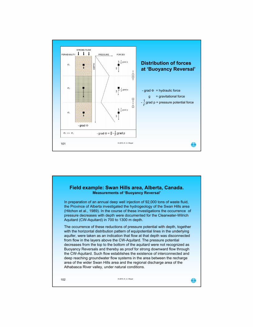
© 2010, K. U. Weyer101
Distribution of forces at ‘Buoyancy Reversal’
- grad = hydraulic force
g = gravitational force
- grad p = pressure potential force
© 2010, K. U. Weyer102
Field example: Swan Hills area, Alberta, Canada.Measurements of ‘Buoyancy Reversal’
In preparation of an annual deep well injection of 92,000 tons of waste fluid, the Province of Alberta investigated the hydrogeology of the Swan Hills area (Hitchon et al., 1989). In the course of these investigations the occurrence of pressure decreases with depth were documented for the Clearwater-Wilrich Aquitard (CW-Aquitard) in 700 to 1300 m depth.
The occurrence of these reductions of pressure potential with depth, together with the horizontal distribution pattern of equipotential lines in the underlying aquifer, were taken as an indication that flow at that depth was disconnected from flow in the layers above the CW-Aquitard. The pressure potential decreases from the top to the bottom of the aquitard were not recognized as Buoyancy Reversals and thereby as proof for strong downward flow through the CW-Aquitard. Such flow establishes the existence of interconnected and deep reaching groundwater flow systems in the area between the recharge area of the wider Swan Hills area and the regional discharge area of the Athabasca River valley, under natural conditions.

© 2010, K. U. Weyer103
Winter view from the town of Swan Hills towards the high regions of the Swan Hills
K. U. Weyer, 20060208
© 2010, K. U. Weyer104
Digital Elevation Model [DEM] of the Swan Hills area, Alberta, one of the places where ‘Buoyancy Reversal’ was measured in the field
The geologic cross-section A-A’ is marked as a red line. At the sites A,B, and C the occurrenceof ‘Buoyancy Reversal’ was determined to occur within the Clearwater-Wilrich aquitard.
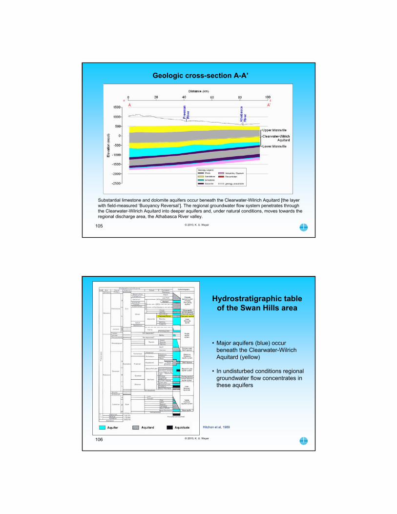
© 2010, K. U. Weyer105
Geologic cross-section A-A’.
Substantial limestone and dolomite aquifers occur beneath the Clearwater-Wilrich Aquitard [the layer with field-measured ‘Buoyancy Reversal’]. The regional groundwater flow system penetrates through the Clearwater-Wilrich Aquitard into deeper aquifers and, under natural conditions, moves towards the regional discharge area, the Athabasca River valley.
© 2010, K. U. Weyer106
Hitchon et al, 1989
Hydrostratigraphic table of the Swan Hills area
• Major aquifers (blue) occur beneath the Clearwater-Wilrich Aquitard (yellow)
• In undisturbed conditions regional groundwater flow concentrates in these aquifers

© 2010, K. U. Weyer107
‘Buoyancy Reversal’within the Clearwater-Wilrich Aquitard
Hitchon et al, 1989
‘Buoyancy Reversal’ atDEM Site A
© 2010, K. U. Weyer
‘Buoyancy Reversal’ atDEM Site B
108
‘Buoyancy Reversal’within the Clearwater-Wilrich Aquitard
Hitchon et al, 1989

© 2010, K. U. Weyer
‘Buoyancy Reversal’ atDEM Site C
109
‘Buoyancy Reversal’within the Clearwater-Wilrich Aquitard
Hitchon et al, 1989
© 2010, K. U. Weyer110
• Sink conditions versus source conditions 111
• Mathematical models by IPCC [7] and Princeton [8] 115
• Effect of deep wells upon fluid flow 118- Microannuli- Deep well abandonment
• Field examples and mathematical models 128- Field example and mathematical model [9]: Hayter field, Provost area, Alberta
- Field example and mathematical model [10]: Freed investigation, TWP 50-51,Rge 14-15 W4M Alberta
Section 10
Geological storage of CO2

© 2010, K. U. Weyer111
Sink conditions versus source conditions
At reservoir sites, conditions would change from sink to source when CO2 is injected. Under EOR (Enhanced Oil Recovery) and CCS (Carbon Capture and Storage) conditions, there will be hydrous flow penetrating the caprock (aquitard) outward. Oil and gas would penetrate capillary seals if the gradient of the pressure potential at the seal exceeds the gradient of the capillary pressure potential.
© 2010, K. U. Weyer112
Schematics of head development during petroleum production, EOR and subsequent CCS
Energy state [hydraulic potential is shown by equivalent freshwater heads [h], where = h * g [energy/mass; L2T-2]

113
Schematic of water flow penetrating hydrocarbon accumulation and caprock
Due to capillary forces, hydrocarbons normally do not penetrate caprock but water does in either normal direction (see slide 23).
© 2010, K. U. Weyer
© 2010, K. U. Weyer114
Hydraulic monitoring and chemical sampling with piezometers and electronic equipment[pressure transducers, electrical conductivity, pH, T, etc.]
Hydraulic monitoring has not yet been considered within CCS work and had also not been considered by the IPCC (2005).
While geophysical monitoring endeavours to identify the actual plumes of liquid CO2, hydraulic monitoring would also allow us to monitor changes in the regional groundwater flow systems, and thereby the migration of the dissolved CO2 plumes.
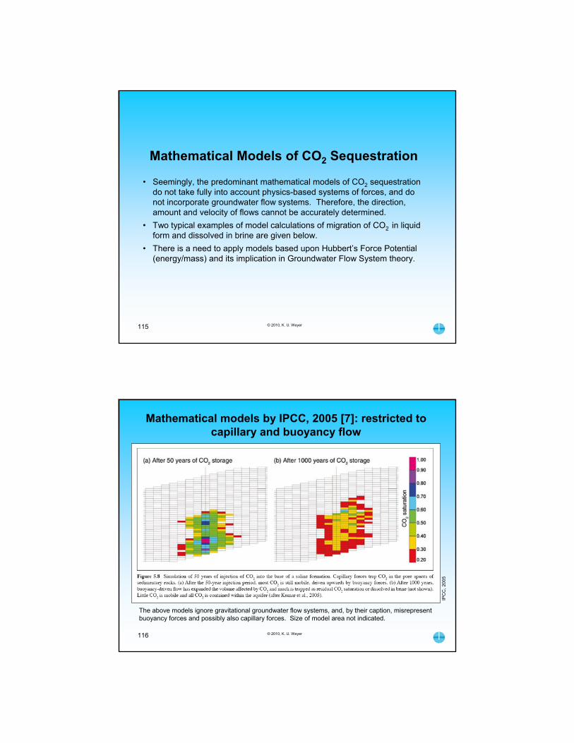
© 2010, K. U. Weyer115
Mathematical Models of CO2 Sequestration
• Seemingly, the predominant mathematical models of CO2 sequestration do not take fully into account physics-based systems of forces, and do not incorporate groundwater flow systems. Therefore, the direction, amount and velocity of flows cannot be accurately determined.
• Two typical examples of model calculations of migration of CO2 in liquid form and dissolved in brine are given below.
• There is a need to apply models based upon Hubbert’s Force Potential (energy/mass) and its implication in Groundwater Flow System theory.
© 2010, K. U. Weyer116
IPC
C, 2
005
Mathematical models by IPCC, 2005 [7]: restricted to capillary and buoyancy flow
The above models ignore gravitational groundwater flow systems, and, by their caption, misrepresent buoyancy forces and possibly also capillary forces. Size of model area not indicated.
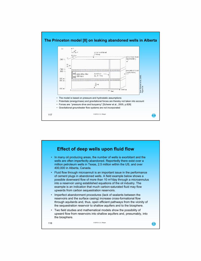
© 2010, K. U. Weyer117
The Princeton model [8] on leaking abandoned wells in Alberta
• The model is based on pressure and hydrostatic assumptions
• Potentials (energy/mass) and gravitational forces are thereby not taken into account
• Forces are: “pressure drive and buoyancy” [Scherer et al., 2005, p.828]
• Gravitational groundwater flow systems are not incorporated
from
Sch
erer
et a
l, 20
05,
Fig
ure
3a
© 2010, K. U. Weyer118
Effect of deep wells upon fluid flow
• In many oil producing areas, the number of wells is exorbitant and the wells are often imperfectly abandoned. Reportedly there exist over a million petroleum wells in Texas, 2.5 million within the US, and over 400,000 in Alberta, Canada.
• Fluid flow through microannuli is an important issue in the performance of cement plugs in abandoned wells. A field example below shows a possible downward flow of more than 10 m3/day through a microannulus into a reservoir using established equations of the oil industry. The example is an indication that much carbon-saturated fluid may flow upwards from carbon sequestration reservoirs.
• Imperfect abandonment procedures (lack of sealants between the reservoirs and the surface casing) increase cross-formational flow through aquitards and, thus, open efficient pathways from the vicinity of the sequestration reservoir to shallow aquifers and to the biosphere.
• Two field studies and mathematical models show the possibility of upward flow from reservoirs into shallow aquifers and, presumably, into the biosphere.
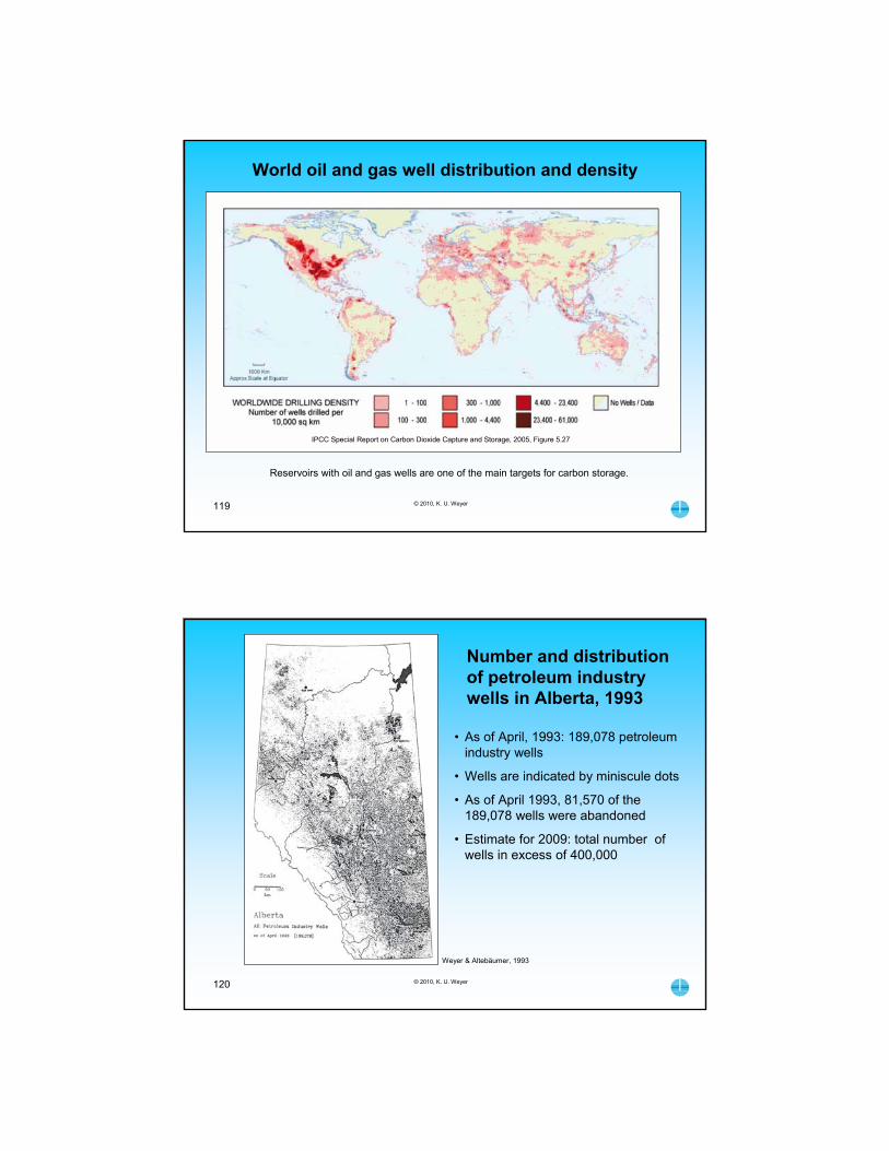
© 2010, K. U. Weyer119
World oil and gas well distribution and density
IPCC Special Report on Carbon Dioxide Capture and Storage, 2005, Figure 5.27
Reservoirs with oil and gas wells are one of the main targets for carbon storage.
© 2010, K. U. Weyer120
Number and distribution of petroleum industry wells in Alberta, 1993
Weyer & Altebäumer, 1993
• As of April, 1993: 189,078 petroleum industry wells
• Wells are indicated by miniscule dots
• As of April 1993, 81,570 of the 189,078 wells were abandoned
• Estimate for 2009: total number of wells in excess of 400,000
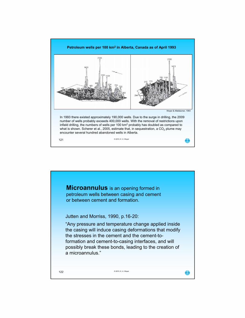
© 2010, K. U. Weyer121
Weyer & Altebäumer, 1993
Petroleum wells per 100 km2 in Alberta, Canada as of April 1993
In 1993 there existed approximately 190,000 wells. Due to the surge in drilling, the 2009 number of wells probably exceeds 400,000 wells. With the removal of restrictions upon infield drilling, the numbers of wells per 100 km2 probably has doubled as compared to what is shown. Scherer et al., 2005, estimate that, in sequestration, a CO2 plume may encounter several hundred abandoned wells in Alberta.
© 2010, K. U. Weyer122
Microannulus is an opening formed in petroleum wells between casing and cement or between cement and formation.
Jutten and Morriss, 1990, p.16-20:
“Any pressure and temperature change applied inside the casing will induce casing deformations that modify the stresses in the cement and the cement-to-formation and cement-to-casing interfaces, and will possibly break these bonds, leading to the creation of a microannulus.”
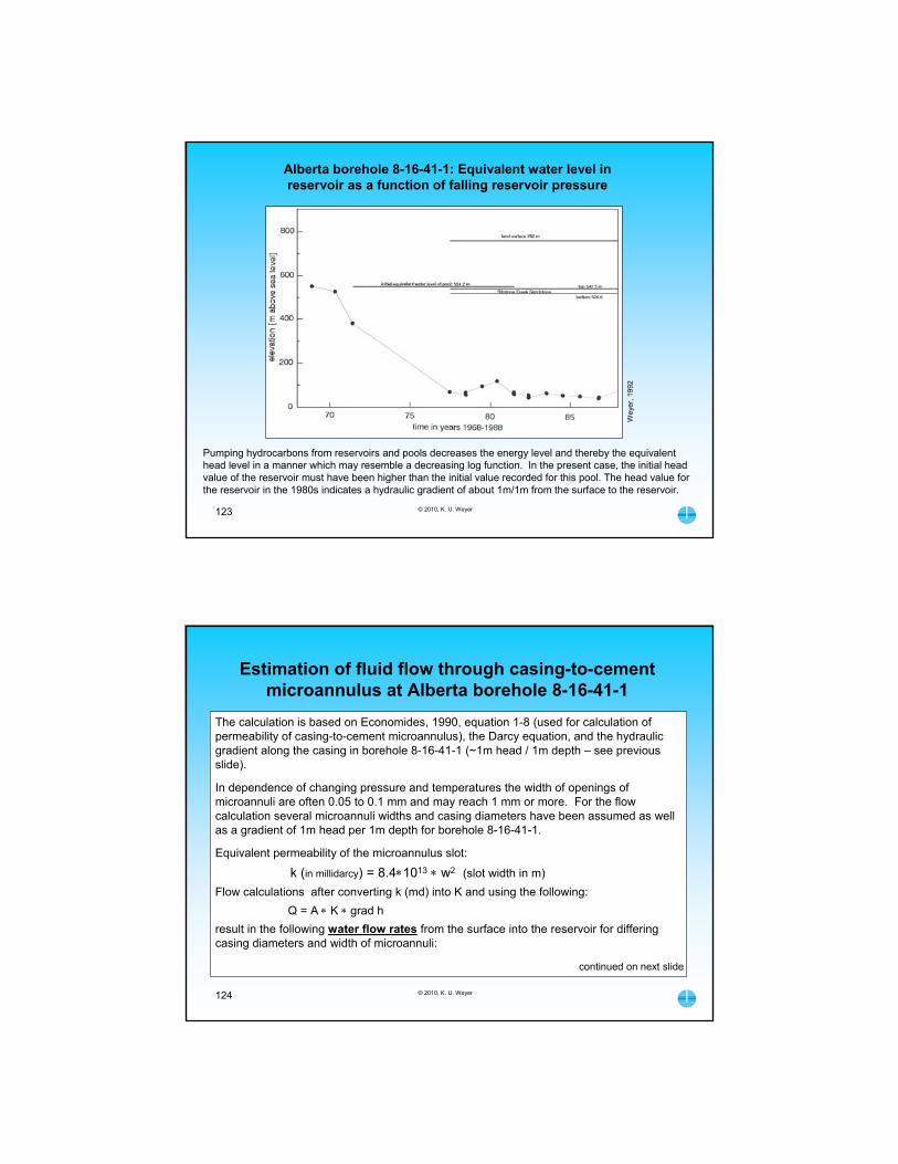
© 2010, K. U. Weyer123
Wey
er, 1
992
Alberta borehole 8-16-41-1: Equivalent water level in reservoir as a function of falling reservoir pressure
Pumping hydrocarbons from reservoirs and pools decreases the energy level and thereby the equivalent head level in a manner which may resemble a decreasing log function. In the present case, the initial head value of the reservoir must have been higher than the initial value recorded for this pool. The head value for the reservoir in the 1980s indicates a hydraulic gradient of about 1m/1m from the surface to the reservoir.
The calculation is based on Economides, 1990, equation 1-8 (used for calculation of permeability of casing-to-cement microannulus), the Darcy equation, and the hydraulic gradient along the casing in borehole 8-16-41-1 (~1m head / 1m depth – see previous slide).
In dependence of changing pressure and temperatures the width of openings of microannuli are often 0.05 to 0.1 mm and may reach 1 mm or more. For the flow calculation several microannuli widths and casing diameters have been assumed as well as a gradient of 1m head per 1m depth for borehole 8-16-41-1.
Equivalent permeability of the microannulus slot:
k (in millidarcy) = 8.41013 w2 (slot width in m)
Flow calculations after converting k (md) into K and using the following:
Q = A K grad h
result in the following water flow rates from the surface into the reservoir for differing casing diameters and width of microannuli:
continued on next slide
© 2010, K. U. Weyer124
Estimation of fluid flow through casing-to-cement microannulus at Alberta borehole 8-16-41-1
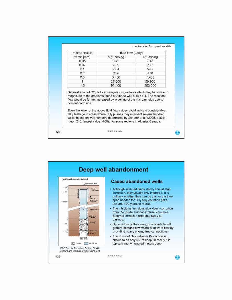
125
continuation from previous slide
© 2010, K. U. Weyer
Sequestration of CO2 will cause upwards gradients which may be similar in magnitude to the gradients found at Alberta well 8-16-41-1. The resultant flow would be further increased by widening of the microannulus due to cement corrosion.
Even the lower of the above fluid flow values could indicate considerable CO2 leakage in areas where CO2 plumes may intersect several hundred wells, based on well numbers determined by Scherer et al. (2005, p.831: mean 240, largest value >700), for some regions in Alberta, Canada.
© 2010, K. U. Weyer
IPCC Special Report on Carbon Dioxide Capture and Storage, 2005, Figure 5.21
126
Cased abandoned wells
• Although inhibited fluids ideally should stop corrosion, they usually only impede it. It is unlikely whether they can do this for the time span needed for CO2 sequestration (let’s assume 100 years or more).
• The inhibiting fluid does slow down corrosion from the inside, but not external corrosion. External corrosion also eats away at casings.
• Upon failure of the casing, the borehole will greatly increase downward or upward flow by providing nearly energy-free connections.
• The ‘Base of Groundwater Protection’ is shown to be only 5-7 m deep. In reality it is typically many hundred meters deep.
Deep well abandonment
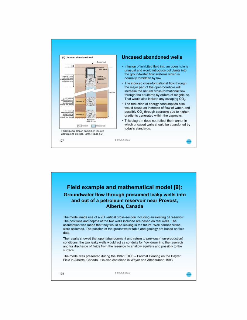
© 2010, K. U. Weyer
IPCC Special Report on Carbon Dioxide Capture and Storage, 2005, Figure 5.21
127
• Infusion of inhibited fluid into an open hole is unusual and would introduce pollutants into the groundwater flow systems which is normally forbidden by law.
• The induced cross-formational flow through the major part of the open borehole will increase the natural cross-formational flow through the aquitards by orders of magnitude. That would also include any escaping CO2.
• The reduction of energy consumption also would cause an increase of flow of water, and possibly CO2 through caprocks due to higher gradients generated within the caprocks.
• This diagram does not reflect the manner in which uncased wells should be abandoned by today’s standards.
Uncased abandoned wells
© 2010, K. U. Weyer128
Field example and mathematical model [9]:Groundwater flow through presumed leaky wells into
and out of a petroleum reservoir near Provost, Alberta, Canada
The model made use of a 2D vertical cross-section including an existing oil reservoir. The positions and depths of the two wells included are based on real wells. The assumption was made that they would be leaking in the future. Well permeabilities were assumed. The position of the groundwater table and geology are based on field data.
The results showed that upon abandonment and return to previous (non-production) conditions, the two leaky wells would act as conduits for flow down into the reservoir and for discharge of fluids from the reservoir to shallow aquifers and possibly to the surface.
The model was presented during the 1992 ERCB – Provost Hearing on the Hayter Field in Alberta, Canada. It is also contained in Weyer and Altebäumer, 1993.

© 2010, K. U. Weyer129
after Weyer, 1992
DEM for 2D-vertical model of groundwater flow into and out of the Hayter Field – Provost area
• DEM – Digital Elevation Model of the investigation area
• Cross-section trace leads from Leane Lake (NE) to Green Glade (SW)
• Dashed lines indicate township boundaries
© 2010, K. U. Weyer130
after Weyer, 1992
ERCB – Provost Hearing: 2D-vertical model of groundwater flow into and out of the Hayter Field – Provost Area
• Local and regional vertical groundwater flow systems in Township 41-1 W4M.
• The deep wells have been assumed to be inadequately sealed (abandoned).
• The model run was based upon permeability contrasts.
• A: ~900 m well with downward flow from recharge area
• B: ~800 m well with upward flow into discharge area
Distance [m]
mas
l A B
caprock (aquitard)
reservoir
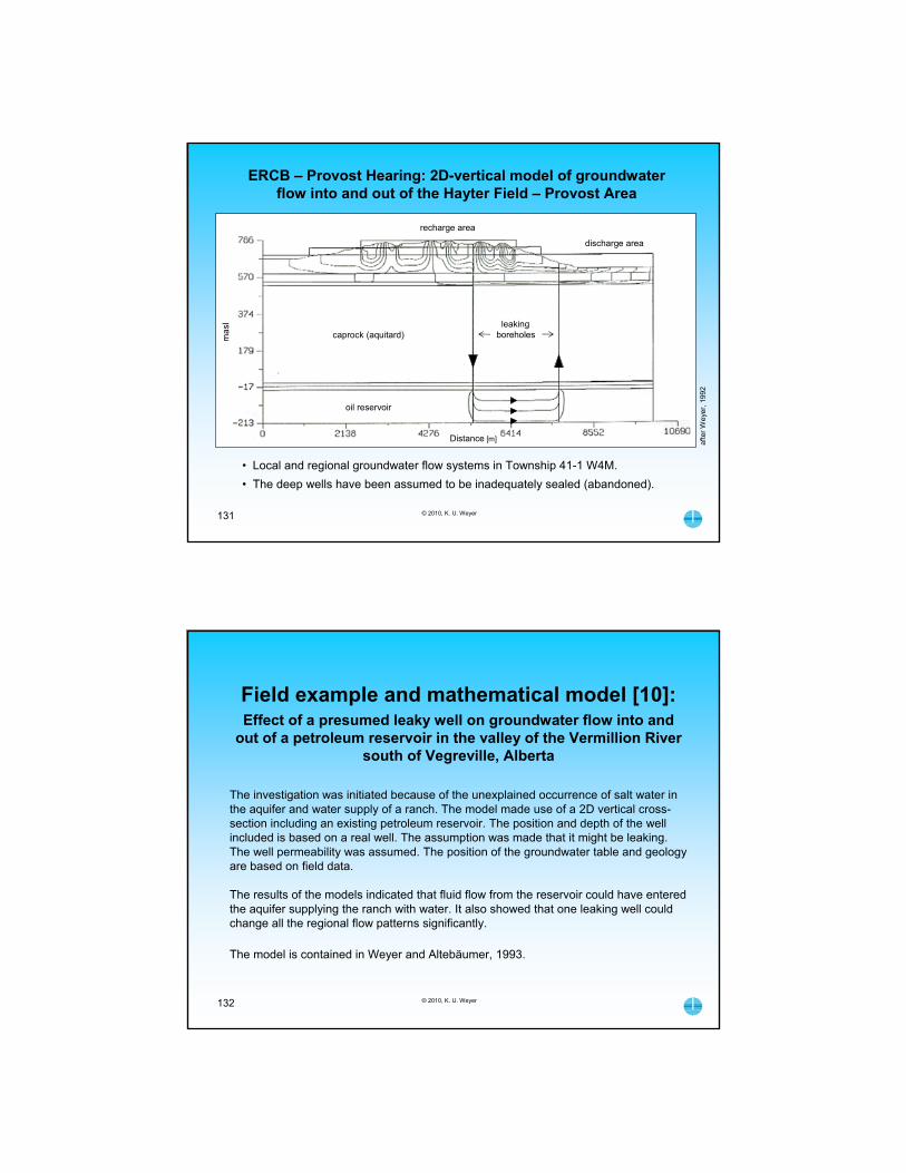
© 2010, K. U. Weyer131
afte
r W
eyer
, 199
2
ERCB – Provost Hearing: 2D-vertical model of groundwater flow into and out of the Hayter Field – Provost Area
Distance [m]
ma
sl leaking boreholes
oil reservoir
caprock (aquitard)
recharge area
discharge area
• Local and regional groundwater flow systems in Township 41-1 W4M.
• The deep wells have been assumed to be inadequately sealed (abandoned).
© 2010, K. U. Weyer132
Field example and mathematical model [10]:Effect of a presumed leaky well on groundwater flow into and
out of a petroleum reservoir in the valley of the Vermillion River south of Vegreville, Alberta
The investigation was initiated because of the unexplained occurrence of salt water in the aquifer and water supply of a ranch. The model made use of a 2D vertical cross-section including an existing petroleum reservoir. The position and depth of the well included is based on a real well. The assumption was made that it might be leaking. The well permeability was assumed. The position of the groundwater table and geology are based on field data.
The results of the models indicated that fluid flow from the reservoir could have entered the aquifer supplying the ranch with water. It also showed that one leaking well could change all the regional flow patterns significantly.
The model is contained in Weyer and Altebäumer, 1993.

© 2010, K. U. Weyer133
DEM for ranch investigation along the Vermillion River, AB
after Weyer and Altebäumer, 1993
The cross-section A-B crosses the valley of the Vermillion River. Posts indicate positions of petroleum wells.
Vermillion River
© 2010, K. U. Weyer134
after Weyer and Altebäumer, 1993
Ranch investigation: 2D-vertical model of groundwater flow directions with and without leaking abandoned gas well
• Upper profile: groundwater flow without abandoned petroleum well.
• Lower profile: effect of leaking petroleum well (in discharge area) on regional groundwater flow. Fluids from the reservoir penetrate into near surface aquifers.
• Depth of reservoir 700 to 900 m.
• The model run was based upon permeability contrasts.
• Contrasts ranged from 1 to 10000 as indicated in the profiles.
mas
lm
asl
Distance [m]

© 2010, K. U. Weyer135
In case of any questions, please do not hesitate to contact the author
K. Udo Weyer, [email protected]
There are also a number of complementing publications on groundwater flow and force fields available at
http://www.wda-consultants.com/papers.htm