Jurnal Ekonomi Malaysia 20 (Disember 1989) 3 -17

Applying a Stochastic Model to the Tenn Structure of Interest Rates in Malaysia

Warren Bailey

ABSTRACT

Malaysia's money and bond markets are increasingly large, complex, and volatile. This paper explains how the Cox, Ingersoll, and Ross model of the term structure of interest rates can be used to value securities and manage risk in such an environment. Computational procedures are discussed and a parameter estimation method is demonstrated using a sample of Malaysian interbank deposit rates.

ABSTRAK

Pasaran wang dan bon di Malaysia adalah bertambah besar, kompleks dan tidak menentu. Kertas ini menerangkan bagaimana model Cox, Ingersoll dan. Ross tentang bentuk struktur kadar bunga boleh digunakan untuk menilai sekuriti dan mengurus risiko dalam suasana yang sedemikian. Turut dlbincangkan ialah prosedur pengiraan dan, kaedah penganggaran parameter yang ditunjuk dengan menggunakan sampel kadar deposit antara bank Malaysia.

INTRODUCTION

Financial markets are among the critical elements of a fully-functioning free market economy. In this regard, Malaysia is a leader among developing countries. Within only a few decades of the nation's birth, the brokerage, financial intermediation, and portfolio management industries are firmly ' established. Trading in corporate stock, foreign currencies, commodity futures contracts, and goverment securities is active and growing.

The economies of North America, Europe, and Japan have recently experienced growth in the size and volatility of their financial markets and an explosion in the trading of complex securities such as option

4 Jurnal Ekonomi Malaysia 20

and futures contracts. In this environment, the effect of volatile interest rates on the value of interest rate sensitive assets and portfolio is consid~rable. Academic researchers have responded by adapting financial theories to produce a variety of techniques for valuing assets and managing portfolios. The usefulness of such techniques is not confined to the financial markets of fully-developed countries. For example, such innovations as the first issues of mortgage-backed securities in Malaysia' require a sophisticated approach to valuation and portfolio analysis.

The growth of financial markets in Malaysia call for the introduction of advanced techniques for the management of portfolios . and the valuation of assets. The purpose of this paper is to introduce a model of the term structure of interest rates, the one-factor model of Cox, Ingersoll, and Ross (1985). Because the model allows for a term structure which varies stochastically through time, it can be adapted to value complex securities (such as mortgage-backed bonds, callable bonds, and options on bonds) and to design strategies to protect bortd portfolio against changes in interest rates.

THE COX, INGERSOLL, AND ROSS ONE-FACTOR MODEL

Cox, Ingersoll, Ross (1985) derive asset pricirig formulas in a single good, single production technology general equilibrium setting. A fundamental result of their analysis ia an expression for the dynamic of r, the yield on an instantaneously-maturing riskless deposit:

dr = k(m - r)dt + (1.../r dz (1)

The instantaneous change in r, dr, has a deterministic component, k(m - r)dt, which indicates that r tends to revert to its "long-run" mean, m, with a speed-of-adjustment of kdt. The instantaneous change in r also has a stochastic component, G'lrdz. This stochastic component consists of the increment of a Brownian motion process, dz, mUltiplied by a constant, (1, times the square root of the current value of r.2

While r represents the yield on an instantaneously-maturing deposit, it does not equal the yield on a longer-maturity riskless instrument.3 Let P(r, t, T) represent the current value (conditional on r) of a zero coupon bond which matures (paying one dollar) at time T in the future. Cox, Ingersoll, and Ross (1985) present a partial differential equation for the value of P:

(2)

Interest Rates in Malaysia 5

In equation (2), the subsripts indicate partial derivatives while g represents the equilibrium risk premium for interest rate risk. Because the value of the zero coupon bond is constrained by unusually simple boundary conditions (the bond can never sell for less than zero or greater than one, and it must pay exact one at maturity), Cox, Ingersoll, and Ross are able to solve the partial differential equation (2). They

. obtain an expression for the value of the zero coupon bond given the current value of r:

P(r, t, T) = A(t, T) exp{-B(t, T) r} (3)

A(t T) = [ 2 h exp{ (h + k + g)(T - t)/2} ]2km1U 2 (3a) , (h + k + g)(exp{ h(T - t) I-I) + 2h

2 (exp (h(T - t)} - I B(t,T) = (h + k + g)(exp{h(T - t)} - 1) + 2h (3b)

h = -V[(k + g)2 + 2cr] (3c)

By taking the natural log of I/p(r, t, T) and dividing by the time until maturity (T - t), we obtain an expression for R(r, t, T), the yield to maturity (or internal rate of return) of zero coupon bond:

R(r, t, T) = [r B(t, T) - In{A(t, T)}]/(T - t) (4)

Given estimates of the parameters k, m, (J, and g, it is straightforward to compute the value P(r~ t, T) for any values of the instantaneous yield, r, and time until zero coupon maturity, T - t, required.

The formula for P(r, t, T) has important uses beyong valuing zero coupon deposits or Treasury bills. Consider the value of a coupon bond: it may be valued as the sum of values of its component parts (coupon payments plus final principal repayment). Each component (a single coupon or principal cash flow) is akin to a zero coupon bond and can be valued using the formula for P(r, t, T). Therefore, we may express the value, B(r, t, T), of a coupon bond as:

B(r, t, T) = I.;=t [coupon • P(r, t, i)] + [principal • P(r, t, T)] (5)

In a related paper, Cox, Ingersoll, and Ross (1981) present closed form solutions for forward and futures contracts for delivery of zero coupon bonds.4 Both forward and futures contracts require delivery of the underlying price. Both have zero initial cost. A distinction between the two is that the price is paid in full at maturity in the case of the

6 Jurnal Ekonomi Malaysia 20

forward contract while any gains or losses are paid incrementally over the life of the futures contract.

The formulas presented in Cox, Ingersoll, and Ross (1981) are as straightforward to evaluate as those for bonds. Let G(r, t, T, s) denote the current forward price for a contract which matures at time T and requires delivery of a zero coupon bond with one dollar face value which matures at time s, where is s greater than T. The formula for the forward price is:

A(t, s) G(r, t, T, s) = A(t, T) exp{ - r[B(t, s)-B(t, T)]} (6)

Let H(r, t, T, s) denote the current futures price for a contract which matures at time T and requires delivery of a zero coupon bond with one dollar face value which matures at time s, where s is greater than T. The formula for the futures price is:

. '. 2km/cY-H (r, t, T, s) = A(T, s) [n/(B(T, s) + n)] •

. { n B(T, s) exp{ - (k + q) (T - t) } exp - r B(T, s) + n (7)

n = [2(k + q)]/[S2(1- exp{- (k + q)(T - t)})] (7a)

In addition to the ease with which the formulas presented above can be evaluated, the existence of closed form solutions facilitates the computation of derivatives. The computation of derivatives is critical to the management of fixed income portfolios.

ESTIMATING THE PARAMETERS REQUIRED BY THE MODEL

Estimation of the parameters k, m, (j, and g presents two problems. First, the dynamics of r, Equation (1), are specified as if r is continously observable when in fact it can only be observed periodically. Second, the interest rate risk premium, g, is unobservable and cannot be estimated from observations of r. To remedy the first problem, we use a discrete time approximation to equation (1):

(8)

et is a random variable distributed normally with mean zero and variance

lcY- while i represents the size of the observation interval. For example,

Interest Rates in Malaysia 7

if r is observed monthly, t equals 1/12. If this discrete time approximation is used as a regression specification, it will have heteroskedastic errors (due to the time-varying -vrt _ 1 term multiplying et) and violate a basic assumption of OLS regression. Therefore, the equation is divided through by the square root of rt _ 1 to yield a regression specification with homoskedastic errors:

(9)

From this equation, we obtain estimates ~ and ~ directly. An estimate of Cf is obtained from the standard deviation of the estimated residual

. " senes, et" To estimate the coefficients of specifications (9), we obtain a time­

series of average end-of-month seven day interbank rates from Bank Negara Malaysia publications.5 This time series, extending from January 1983 to December 1987, is used to proxy for rt, the yield on an instantaneously-maturing deposit. The resulting regression estimate is:6

(rt - rt_l)/-vrt_l = 0.0127/-Vrt_1 - 0.1816 -vrt_l (10)

(.704) (.108)

Standard errors are reported in parentheses beneath each coefficient estimate. The regression has an R2 of 0.053, standard deviation of residuals of 0.0111, atJd autocorrelation of residuals of ~.245. Adjusting for the t factor of 12, the resulting parameter estimates to input to the

. " " " model are K = 2.179, m = 0.070, and Cf = 0.038.7 The parameter estimates imply that the seven day interbank rate has a long-run mean of 7% and tends to revert to that mean at a rate of about 218% per year.

To solve the second problem of estimating the risk premium, g, we will obtain as estimate conditional on Q, ~, and &. Returning to Bank Negara published records, we take a matching end-of month time-series of three month interbank rates for January 1983 to December 1987. Represent this series as Yt. We then predict each value in the series using the formula for the yield-to-maturity on a three-month zero coupon deposit, equation (4). t ~, and ~, along with a guess at g, are plugged into the formula for R(rt, t, t + 0.25). We then compute the average squared relative error between actual and predicted yields:

6~L ~~~3 [Yj - R(rj, i, i + 0.25]/Yj (11)

We continue to try various values of g until finding one which minimizes equation (11). For this particular dataset, the procedure yields g = .058.

8 Jurnal Ekonomi Malaysia 20

NUMERICAL METHODS FOR V ALUING SECURITIES

Given the closed form solutions provided in Cox, Ingersoll, ~d Ross (1981, 1985), ordinary bonds and future delivery contracts for zero coupon bonds can be easily valued ina stochastic interest rate environment. The key to obtaining these formulas is to solve the fundamental partial differential equation for asset prices in the Co~, Ingersoll, and Ross economy:

1 ' "2 dr V rr + [k(m - r) - gr] Vr + VI - rV + c = 0 (12)

Equation (12) is a generalized from of Equation (2) in that it includes a term, c, representing a coupon flow from the asset whose price is V. The equation is solved with the boundary conditions appropriate to the particular security being valued.

Unfortunately, most problems have boundary conditions which, when combined with Equation (12), cannot be solved for a closed form solution. However, numerical solutions can be applied. This will not yield a formula and, furthermore, requires the use of a computer and carefully-prepared program. However, a numerical method can give a valu~ for any security given parameter estimates and a specific value or f.

Smith (1978) provides an excellent introduction to numerical methods while McDonald (1978) offers a step-by-step guide to applying numerical methods to implement the cox, Ingersoll, and Ross model. While a detailed discussion of numerical methods is beyond the scope of this introductory paper, the basic idea is as follows. First, replace the partial derivatives in Equation (12) with finite differences:

V = [V(r. l' t) - V(r. l' t)]/[r. 1 - r. 1] r J + J - J + J-

V rr = [V(rj + l' t) - 2 V(rj, t) + V(rj _ l' t)]1

[(1/2)(rj + 1 - rj _ 1)]2

VI = [V(r., t + 1) - V(r., t)]/[(t + 1) - t] J J

(13a)

(13b)

(13c)

Next, solve the equation iteratively, working backwards from the terminal boundary condition and imposing other boundary conditions at each step until the security's current value is obtained.

To illustrate the type of information a numerical procedure can produce, Table 1 includes values of bonds and comparable callable

TABLE 1. Prices for Callable Bonds Simulated by the Cox, Ingersoll, and Ross One-Factor Model a

Callable Bondb

Non-Callable Bond Instantaneous Time until Interest Maturity Bond First Callable Rate, r in years Coupon Price in Years Price

0.01 10 7% 103.9~3 5 103.308 0.04 10 7% 102.601 5 101.975 0.07 10 7% 101.278 5 100.660 0.10 10 7% 99.704 5 99.096 0.13 10 7% 97.437 5 96.844

0.04 10 7% 102.601 3 101.677 0.07 10 7% 101.278 3 100.367 0.10 10 7% 99.704 3 98.808

0.04 10 7% 102.601 8 102.355 0.07 10 7% 101.278 8 101.035 0.10 10 7% 99.704 8 99.465

0.04 20 7% 103.297 15 102.980 0.07 20 7% 101.964 15 101.652 0.10 ~O 7% 100.379 15 100.072

0.04 10 4% 80.596 5 80.596 0 .. 07 10 4% 79.547 5 79.547 0.10 10 4% 78.294 5 78.294

0.04 10 10% 124.605 5 114.879 0.07 10 10% 123.006 5 113.409 0.10 10 10% 121.112 5 111.672

0.01 10 7% 104.399 * 5 102.379* 0.04 10 7% 103.072 * 5 101.077 * 0.07 10 7% 101.770* 5 99.801 * 0.10 10 7% 100.479 * 5 98.536* 0.13 10 7% 99.206 * 597.289*

a Bonds have a face value of $1 00. Calculation are based on parameter estimates ofk = 2.179, m= 0.070, and g = 0.058. All calculation are based on G = 0.038 except for those cases marked with a '*', which are based on G= .38. b The callable bond has the same maturity and coupon as the non-callable. bond.

TABLE 2. Prices for Bond Options simulated by the Cox, Ingersoll, and Ross One-Factor Model a

Instant- Underlying Bond Options aneous Interest Maturity Life Strike Call Put Rate, r in Years Coupon Price in Years Price Price Price

0.01 10 7% 103.943 0.5 96 7.943 <0.001 0.04 10 7% 102.601 0.5 96 6.601 <0.001 0.07 10 7% 101.278 0.5 96 5.278 <0.001 0.10 10 7% 99.704 0.5 96 4.452 <0.001 0.13 10 7% 97.437 0.5 96 3.478 0.175

0.01 10 7% 103.943 0.5 98 5.943 <0.001 0.04 10 7% 102.601 0.5 98 4.601 <0.001 0.07 10 7% 101.278 0.5 98 3.289 <0.001 0.10 10 7%. 99.704 0.5 98 2.614 0.007 0.13 10 7% 97.437 0.5 98 2.027 0.864

0.01 10 7% 103.943 0.5 - 100 3.943 <0.001 0.04 10 7% 102.601 0.5 100 2.601 <0.001 0.07 10 7% 101.278 0.5 100 1.314 <0.001 0.10 10 7% 99.704 0.5 100 0.808 0.296 0.13 10 7% 97.437 0.5 100 0.401 2.592

0.01 10 7% 103.943 98 5.943 <0.001 0.04 10 7% 102.601 98 4.601 <0.001 0.07 10 7% 101.278 98 3.299 <0.001 0.10 10 7% 99.704 98 2.876 0.011 0.13 10 7% 97.437 98 2.726 0.864

0.01 10 7% 103.943 100 3.943 <0.001 0.04 10 7% 102.601 100 2.601 <0.001 0.07 10 7% 101.278 100 1.333 <0.001 0.10 10 7% 99.704 100 1.050 0.296 0.13 10 7% 97.437 100 0.890 2.592

0.01 10 7% 104.399 * 0.5 100 4.399* 0.093 '" 0.04 10 7% 103.072. * 0.5 100 3.103 * 0.204* 0.07 10 7% 101.770 * 0.5 100 2.410 * 0.388 * 0.10 10 7% 100.479 * 0.5 100 1.957 * 0.685 * 0.13 10 7% 99.206* 0.5 100 1.614 * 1.170 *

a Bonds have a face value of$1 00. Calculation are based on parameter estimates ofk = 2.179, m = 0.070, and g = 0.058. All calculations are based on G = 0.038 except for tl,tose cases marked with a '*', which are based on G= .38.

Interest Rates in Malaysia 11

bonds. A callable bond differs from a regular bond in that the issuer of the bond can, at pre specified times, choose to refund the principal value of the bond early, thus retiring the debt. The chance that the bond may be called tends to reduce its value relative to the non-callable bond, as indicated by the table. The table shows that the degree to which the value is reduced varies wi~ely with the maturity of the bond, time until it may be called, and the current interest rate, r.

Table 2 includes values of put and call options on bonds. These contracts allow the holder to either sell ("put") or buy ("call") the underlying bond at a pre specified price ("strike") prior to the time the contract expires. The option premium is the difference between the option's current value and its value if exercised immediately. Consider the last line in the table. Given a strike price of $100 and a current bond price of only $99.206, the call option should not be exercised: a rational investor will not pay $100 for a bond worth only $99.206. However, the call option still has value ($1.614) because it is possible that the bond price will increase beyond $100 and allow the . call to be exercised profitably.

Throughout Tables 1 and 2, it is apparent that volatility has an important effect on securities. The last several lines of each of Tables 1 and 2 recompute bond and option values based on a = 0.38, rather than 0.038. The resulting values are very different from the otherwise indentical values computed with a= 0.038. Differences between callable and regular bonds and levels of put and call prices are greater for the larger level of volatility.

USING THE MODEL TO MANAGE INTEREST RATE RISK

Aside from valuing various securities, the Cox, Ingersoll, and Ross model can be used to manage a portfolio against interest rate risk.8

Given the closed form solutions for bond, forward, and futures prices, we can compute the partial derivatives of these price with respect to r. For the zero coupon bond differentiate equation (3) to obtain:

Pr (r, t, T) = -B(t, T) P(r, t, T) (14)

For the coupon bond, differentiate equation (~) to obtain:

Br(r, t, T) = L;=t [coupon • Pr(r, t, i)] + [principal • Pr(r, t, T)] (15)

For forward and futures prices, differentiate equations (6) and (7) to obtain:

12 Jurnal Ekonomi Malaysia 20

Gr(r, t, T, s) = - [B(t, s) -B(t, T)] G(r, t, T, s) (16)

H ( t T ) = _ n B(T, s) exp{ - (k + q)(T - t)} H( T) (17) r r" ,s B(T, s) + n r, t, ,s

In the case of callable -bonds, options on bonds, and other complex securities, there is no closed form solution. to the valuation equation. Therefore, we cannot compute derivatives directly. However, we can use a numerical procedures to get an estimate of the derivative at a particular value of r. Let V(r, t) represent the price of the security estimated by numerical methods and let r' represent the particular value ofr at which we wish to estimate the derivative Yr. We use a differencing approach to estimate the derivative:

Vr(r', t) ~ [V(r' + 0.01, t) - V(r' - 0.01, t)]/0.02 (18)

In effect, we plug into the numerical' formula values' of r which surround r', then produce values of the security and compute an approximation to the derivative using defferences in V(r, t) and r.

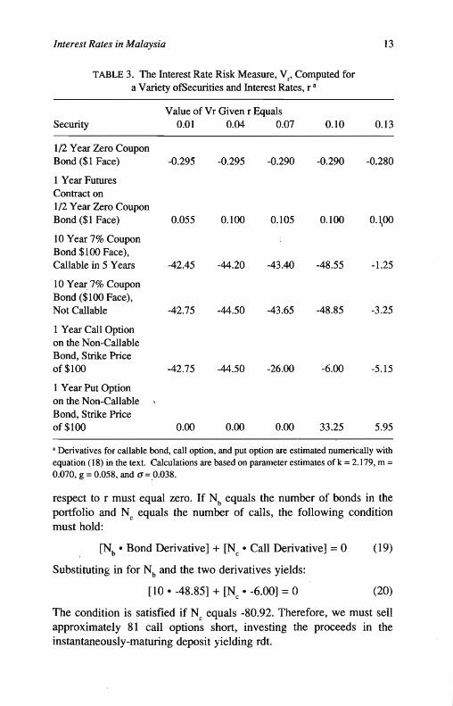
The derivative is a measure of the degree to which a security's price changes in response to a change in the interest rate, r. It is, in effect, the measure of the security's interest rate risk. Table 3 presents some calculation of these derivatives for several types of hypothetical securities. Consider the value of -48.85 reported for the ten year coupon bond when the interest rate is 10%. This mean that, if the interest rate goes from 0.10 to 0.11, the change in the bond's price will be approximately minus fifty cents (-48.85 times 0.01). It is clear from the table that the behaviour of the derivative varies widely across securities. Note also that the derivative is different for different values of r. Furthermore, the derivative changes as time passes and the maturity (or expiration) of the security becomes less distant.

Given the derivatives for various securities" Boyle (1978) details how to modify a bond portfolio to protect it against interest rate risk. We will consider examples based on the derivatives presented in Table 3. Suppose we begin with a portfolio of ten of the ten year 7% coupon bonds. Let the current value of r be 0.10. An increase in interest rates will reduce the value of the portfolio. Therefore, we wish to add additional positions in securities to the portfolio so as to offset the potential loss.

Consider adding some call options to the portfolio. To be hedged against interest rate risk, the derivative of the portfolio's value with

Interest Rates in Malaysia 13

TABLE 3. The Interest Rate Risk Measure, Vr, Computed for

a Variety ofSecurities and Interest Rates, r a

Value of Vr Given r Equals Security 0.01 0.04 0.07 0.10 0.13

1/2 Year Zero Coupon Bond ($1 Face) -0.295 -0.295 -0.290 -0.290 -0.280

1 Year Futures Contract on 1/2 Year Zero Coupon Bond ($1 Face) 0.055 0.100 0.105 0.100 0.\00

10 Year 7% Coupon Bond $100 Face), Callable in 5 Years -42.45 -44.20 -43.40 -48.55 -1.25

10 Year 7% Coupon Bond ($100 Face), Not Callable -42.75 -44.50 -43.65 -48.85 -3.25

1 Year Call Option on the Non-Callable Bond, Strike Price of $100 -42.75 -44.50 -26.00 -6.00 -5.15

1 Year Put Option on the Non-Callable Bond, Strike Price of $100 0.00 0.00 0.00 33.25 5.95

a Derivatives for callable bond, call option, and put option are estimated numerically with equation (18) in the text. Calculations are based on parameter estimates of k = 2.179, m = 0.070, g = 0.058, and 0'=0.038.

respect to r must equal zero. If Nb equals the number of bonds in the portfolio and Nc equals the number of calls, the following condition must hold:

[Nb • Bond Derivative] + [Nc • Call Derivative] = 0 (19)

Substituting in for Nb and the two derivatives yields:

[10 • -48.85] + [Nc • -6.00] = 0 (20)

,The condition is satisfied if Nc equals -80.92. Therefore, we must sell approximately 81 call options short, investing the proceeds in the instantaneously-maturing deposit yielding rdt.

14 Jurnal Ekonomi Malaysia 20

Similar calculations indicate how many zero coupon bond futures contracts would hedge the bond portfolio. Letting Nf denote the number of futures contracts, the condition to be satisfied is:

[Nb • Bond Derivative] + [Nf • Futures Derivative] = 0 (21)

Substituting for the known quantities and solving yields Nf equal to 4855. Therefore, future.s contracts on zeros with a total face value of $4855 can be used instead of call options. The advantage to this strategy is that futures require no initial cash flow. Alternatively, consider the number of puts needed to hedge the portfolio of ten bonds. Calculations similar to those performed previously yield 14.60 puts as the optimal number to hedge the portfolio.

For all these strategies, the optimal composition of the hedging portfolio changes as r varies, time passes, and the derivatives change. Ideally, the portfolio should be rearranged frequently to reflect current values of the derivatives. However, it may be optimal to rearrange infrequently so as to avoid brokerage fees and other trading costs.

AN INTRODUCTION TO OTHER TERM STRUCTURE MODELS

The Cox, Ingersoll, and Ross model has stimulated other authors to produce more complex asset pricing models of the stochastic interest rate environment. We will introduce a few of th~se in this section.

Brennan and Schwartz (1979) point out two potentially unrealistic features of the Cox, Ingersoll, and Ross approach. First, it relys on only a single variable, r, to generate a stochastic interest rate environment. Second, that single variable reverts to a target, m, which is unchanging through time. Brennan and Schwarts (1979) propose a two variable model similar to the following:

dr = k(1 - r)dt + G rdz (19a)

dl = l(s'2 + s'g + 1 - r)dt + <ildz' (19b)

I represent the yield on a coupon bond with an infinite maturity (known as ·a "con sol" bond), d is a parameter, and dz' is the increment of a second Brownian motion process, which has correlation pdt with dz. Essentially, the return on an instantaneously-maturing deposit, r, now reverts to a "moving target", 1, rather than the fixed target, . m, in the Cox, Ingersoll, and Ross model. Furthermore, these are now two distinct,

Interest Rates in Malaysia 15

not necessarily correlated sources of uncertainty, r and 1. This allows the term structure of interest rates to vary in more complex ways than the Cox, Ingersoll, and Ross model. Unfortunately, the mathematics of the model require complicated numerical solutions.

Other authors have adapted the cox, Ingersoll, and Ross model to pricing of mortgage-backed securities with the following specification of uncertainty factors:

dr = k(m - r)dt + aVrdz (20a)

dS = m'Sdt + (J' Sdz' (20b)

In this case, the Cox, Ingersoll, and Ross interest rate dynamics are retained: equation (20a) is identical to equation (1). However, a second equation is added to represent the dynamics of S, the value of the property underlying the mortgage. Given that a drop in property values can cause a default on a mortgage and thus affect the value of mortgage­backed securities, the addition of equation (20b) may make the model more realistic and accurate. Hendershort and Van Order (1987) provide a review of such models. Unfortunately, complex numerical solutions are required. Bailey (1987) discusses numerical solution techniques for a similar problem in option pricing.

Most recentlu, papers, by Ho and Lee (1986) and Health, Jarrow, and Morton (1988) have introduced an entire new class of term structure models. Rather than"assume that the term structure is driven soley by one or two uncertainty variables, these new models start with the entire

. term structure of zero coupon bond yields as the uncertainty vector. While even a cursory description of these models is beyond the scope of this paper, these models may prove to be of great use because they build upon the entire initially observed term structure (not just r, or r and 1) and can be implemented with relatively simple computer programs.

CONCLUSION

This paper has briefly illustrated the use of the one-factor model of Cox, Ingersoll, and Ross (1985) in valuing securities and managing interest rate risk in a stochastic terin structure environment. The growth of securities trading and the emergence of markets for complex securities increases the importance of these activities and enhances the potential usefulness of this model. This paper is not intended to advocate the

16 Jurnal Ekonomi Malaysia 20

Cox, Ingersoll, and Ross model as the best possible way to model Malaysia's term structure of interest rates, value Malaysian securities, or manage fixed income portfolios in Malaysia. A variety of models, computational techniques, and parameter estimation methods have appeared in the academic literature and are gradually being assessed and, in many cases, adopted by progressive investment professionals. This paper should be thought of as merely an introduction to the potentially useful applications of stochastic term structure models.

ACKNOWLEDGEMENT

I thank Mr. K wan Kwong Seong of the Economics Department of Bank Negara Malaysia for supplying data and providing other assistance with this project'.

NOTES

I The national mortgage corporation of Malaysia; Cagamas Bhd., become operatio­nal in October 1987. Cagamas has purchased housing loans held by fmancial institutions and the government and has issued mortgage-backed bonds. Valuing mortgages is particularly complex due to both contractual features (prepayment, default) and interest rate risk. See Dunn and McConnell (1981), Hendershoot and Van Order (1987), and McDonald (1987).

2 For an introduction to the use of continuous time stochastic models in economics see Merton (1971) and Fischer (1975).

3 It is important to note that the formulas apply only to riskless bonds where there is no probablity of default on the payments promised by the issuer. Furthermore, the formulas are derived in an economy where there is no money (only a single consum­ption 'good) so tI;1ere is no 'inflation and no distinction between real and nominal rates.

4 Such contracts are important risk management tools and already trade on established futures exchanges. Futures on U.S. Treasury bills trade in Chicago while futures on Eurodollar deposits trade in Chicago, London, and Singapore.

S In using the models and estimating parameters, all rates should be expressed as fractions, not as percentages. For example, an interest rate of three percent should be expressed as "0.03", not as "3.0".

6 The use of monthly data from a five year period is only intended to illustrate how the parameter estimation might be conducted. For example, better results might be obtained with weekly observations from only the most recent year, or by using a maximum likelihood or method-of moments estimator.

7 Multiply 0.1816 by 12 to get t: Divide 0.0127 by 0.1816 to get (h. Multiply 0.0111 by the V 12 to get ~

8 Note that traditional risk management based on "duration" cannot be applied to complex securities such as callable bonds, mortgages, and options. Furthermore, the assumption underlying duration may be inconsistent with an arbitrage-free capital market.

See the articles contained in Kaufman, Bierwag, and Toevs (1983).

Interest Rates in Malaysia 17

REFERENCES

Bailey, W. B. 1987. An empirical investigation of the market for comex gold futures options. Journal of Finance 42: 1187-94.

Bank Negara Malaysia. Quarterly Review. Various issues. Boyle, P. P. 1978. Immunization under stochastic models of the term structure,

Journal of the Institute of Actuaries 105: 177-87. Brennan, M. J. & Schwart, E. S. 1979. A continuous time approach to the

pricing of bonds. Journal of Banking and Finance 3:133-55. Brennan, M. J. & Schwart, E. S. 1982. An equilibrium model of bond pricing

and a test of market efficiency . Journal of financial and Quantitative Analysis 16: 301-329.

Cox, J. C., Ingersoll, J. E., & Ross, S. A. 1.981. The relation between forward and futures prices. Journal of Financial Economics 9: 321-46.

Cox, J. c., Ingersoll, J. E. & Ross, S. A. 1985. A theory of the term structure of interest rates. Econometrica 53: 385-407.

Dunn, K. B. & McConnell, J. J. 1981. Valuation of GNMA mortgage-backed securities. Journal of Finance 35: 599-616.

Fischer, S. 1975. The demand for index bonds. Journal of Political Economy 83: 509-34.

Heath, D., Jarrow, R., & Morton, A. 1988. Bond pricing and the term structure of interest rates: The binomial approximation. Unpublished Cornell University working paper.

Hendershott, P. H & Van Order, R. 1987. Pricing mortgages: An interpretation of the models and results. Journal of Financial Services Research 1: 77-111.

Ho, T. S. & Lee S. 1986. Term structure movements and pricing interest rate contigent claims. Journal of Finance 41: 1011-28.

Ingersoll, J. E., Skelton, J., & Weil, R.L., 1978. Duration forty years later. Journal of Financial and Quantitative Analysis 13: 627-50.

Kaufman, G., Bierwag, G. o. &. Toevs A., ed. 1983. Innovations in Bond Portfolio Management: Duration Analysis and Immunization. JAI Press: Greenwich, connecticut, U. S .A.

McDonald, Gregor, 1987. A note on the methods underlying bond and MBS

arbitrage pricing models. Virginia Essays in Economics 7: 18-52. Merton, R. 1971. Optimum consumption and portfolio rules in a continuous

time model. Journal of Econpmic Theory 3: 373-413. Smith, G. D. 1978. Numerical Solution of Partial Differential Equations: Finite

Difference Methods. Claredon Pre,ss: Oxford.

Faculty of Finance Ohio State University 1775 College Road Columbus, OH 43210-1309 USA