applied parallel coordinates for logs and network traffic attack analysis

J Comput Virol (2010) 6:1–29DOI 10.1007/s11416-009-0127-3

ORIGINAL PAPER

Applied parallel coordinates for logs and network trafficattack analysis

Sebastien Tricaud · Philippe Saadé

Received: 20 December 2008 / Accepted: 17 July 2009 / Published online: 27 August 2009© Springer-Verlag France 2009

Abstract By looking on how computer security issues arehandled today, dealing with numerous and unknown events isnot easy. Events need to be normalized, abnormal behaviorsmust be described and known attacks are usually signatures.Parallel coordinates plot offers a new way to deal with sucha vast amount of events and event types: instead of workingwith an alert system, an image is generated so that issuescan be visualized. By simply looking at this image, one cansee line patterns with particular color, thickness, frequency,or convergence behavior that gives evidence of subtle datacorrelation. This paper first starts with the mathematical the-ory needed to understand the power of such a system andlater introduces the Picviz software which implements partof it. Picviz dissects acquired data into a graph descriptionlanguage to make a parallel coordinate picture of it. Its archi-tecture and features are covered with examples of how it canbe used to discover security related issues.

Keywords Visualization · Parallel coordinates ·Data-mining · Logs · Computer security

A picture a day keeps the doctor away.

S. TricaudHoneynet Project French Chapter, 69 rue Rochechouart,75009 Paris, Francee-mail: [email protected]

P. Saadé (B)Lycée la Martinière Monplaisir, Laboratoire de Mathématiques,41, rue Antoine Lumière, 69372 Lyon Cedex 08, Francee-mail: [email protected]

1 Introduction

This paper covers how visualization techniques based onparallel coordinate plots (abbreviated as //-coords) canenhance the computer security area.

It is common to have thousands lines of logs a day ona single machine. With private networks of hundreds of com-puters over complex topologies, this really represents a hugeload of information. How can one separate the important partof the information from the unimportant one?

To deal with that issue, administrators, most of the time,use tools such as Prelude LML,1 OSSEC2 or similar softwarethat are often based on signatures. Besides signatures basedtools, they also use anomaly based tools, that are classifyingthe information after a learning phase. One example is spa-massassin,3 which does a great job at removing spam out ofour mailboxes. Over the years, these tools have proven anindisputable efficiency.

However, something missing today is dealing with dataexactly as it is. There is often more to see than just the partof the data having a matching threshold of signature. That’swhy computer visualization is a good choice!

Computer visualization is a neat way to see the picture ofwhat is really happening and can, in some cases, handle a lotof information. As //-coords can handle multiple dimensionsand an infinity of events, it became a natural choice to writea software being able to automate those graphs creation. Thissoftware is called Picviz.

In the first part of this paper, we will introduce the verybasic facts about //-coords. We will explain in the most sim-ple terms the fundamentals of //-coords as a mathematical

1 http://www.prelude-ids.org.2 http://www.ossec.net.3 http://spamassassin.apache.org.

123

http://www.prelude-ids.org

http://www.ossec.net

http://spamassassin.apache.org

2 S. Tricaud, P. Saadé

theory. The first important results will be given, withoutassuming from the reader a heavy mathematical background.

In the second part, we will present Picviz in its overallarchitecture and then in greater detail.

The last part of this article will be devoted to real-lifeexamples.

We will first discuss the case of giant log files of Cray sys-tems, whose syntax was unknown to the authors and gave achallenging playground for finding important events withoutusing any pre-existing signatures or tools of any kind.

Then, we will consider the particular case of Botnetattacks. It came out that //-coords and Picviz can help indetecting and characterizing these malicious threats. And wewill explain how in the last section of this paper.

Examples including Apache access.log file and wirelessLAN traffic monitoring will also be given.

2 A short mathematical introduction to parallelcoordinates

2.1 Cartesian and parallel point of view

Imagine one has to collect elementary events of a given type(temperatures of all capitals of Asia, network traffic on a net-work adapter, etc.). Let’s suppose that each given elementaryevent carries N kinds of information and that N is not small(greater than 4). Since it is not easy to plot vectors belong-ing to a space of more than 3 dimensions in a 3 dimensionalphysical space (not counting the time), it becomes necessaryto adapt the representation technique.

In an N -dimensional vector space E , one needs a basisof N vectors. Then each vector �u ∈ E corresponds to anN -tuple of the form (x1, x2, . . . , xn). In the usual euclideanspace of dimension N , denoted R

N , the canonical basis isorthogonal, which means that axes are considered pairwiseperpendicular (Fig. 1).

This is the usual cartesian representation of R3 and it

corresponds to our everyday life experience of our ambientspace! But since it is impossible to draw more than 3 per-pendicular axes in a 3 dimensional physical space, the ideabehind //-coords is to draw the axes side by side, all parallel

Fig. 1 Orthogonal basis in R3

Fig. 2 Four axes

Fig. 3 Four axes and a vector

to a given direction. It is then possible to draw all these axesin a 2d plane (Fig. 2):

For example, the vector �u = (0.6, 1.6,−0.8, 1.2) ∈ R4

should show up as (Fig. 3).That point of R

4 has become a polygonal line in //-coords!At first sight, it might seem that we have lost simplicity.

Of course, on one side, it is obvious that many points willlead to many polygonal lines, overlapping each other in avery cumbersome manner. But on the other side, it is a factthat certain relationships between coordinates of the pointcorrespond to interesting patterns in //-coords.

It is the aim of this short mathematical introduction topresent some elementary patterns that can be observed andto prepare the reader for the definition of geometrical invari-ants (in //-coords) of simple subspaces of R

N such as lines,planes and p-subspaces (sometimes called p-flats).

2.2 Trivial hyperplanes

The usual definition of an affine hyperplane in RN is that

it is the set of vectors −→u = (x1, x2, . . . , xN ) satisfying anaffine relationship of the form

α1x1 + α2x2 + · · · + αN xN = β

where all coefficients α1, . . . , αN and β are real numbers andα1, . . . , αN are not zero all together.

That hyperplane is a vector hyperplane or simplya hyperplane if β = 0 which geometrically means that itpasses through to origin O = (0, 0, . . . , 0).

For example, in the usual plane R2, the relationship

α1x1 + α2x2 = β, where (α1, α2) �= (0, 0)

123

Parallel coordinates, logs and network traffic attack analysis 3

Fig. 4 A line in R2

Fig. 5 A coordinate line and a trivial line in R2

characterizes a line orthogonal to vector −→n = (α1, α2)

(Fig. 4).Naturally, in R

3, the cartesian equation

α1x1 + α2x2 + α3x3 = β, where (α1, α2, α3) �= (0, 0, 0)

defines a plane having −→n = (α1, α2, α3) as normal vector.Hyperplanes generalize these geometric objects in higher

dimension and are precisely the (N − 1)-affine subspaces ofR

N .Trivial hyperplanes are those which can be defined by

an equation of the form

xi = b

for a fixed given index i .In such a case, that hyperplane is simply parallel to the ith

coordinate hyperplane having equation xi = 0 (Fig. 5).In //-coordinates, such trivial hyperplanes are very easy

to recognize since one coordinate is constant (Fig. 6):This is the first simple pattern to show up in //-coordi-

nates. For example, if one studies a set of TCP/IP packets,one can assign to the first axis the source IP address and tothe second axis the destination port. It is then obvious that inan attack such as DOS on port 80 (www) of a server comingfrom many different machines, such a structure is going toappear. And even with much more than two axes involved,if one of them represents destination port, the above patternwill still be there, and easy to notice.

Fig. 6 A trivial hyperplane in R4

Now that we have seen that trivial hyperplanes are easyto detect in //-coordinates, we must consider nontrivial ones.Are they so easy to discover? For example, let’s say you have10000 points scattered on a fixed affine hyperplane H in R

5.Will the //-coordinates plot of these 10000 points present atrivial pattern that can be seen at first glance? The definitiveanswer is No! or, more precisely, Not yet!.

So, do not despair! In the following section, we will try toexplain in the most simple terms what can be seen and howit can be seen using //-coordinates.

3 A detailed overview of some basic facts of parallelcoordinates

3.1 Notations and conventions

As said earlier, all //-coordinates plots are drawn on a2-dimensional plane. To keep things simple, all the axes willbe drawn vertically. The plane on which they are drawn isequipped with a usual cartesian coordinate system, denoted

R// = (O,−→ı ,

−→j )

where (−→ı ,

−→j ) is an orthonormal basis (Fig. 7).

A point M in that plane will have its coordinate relativeto R// given by

M = (x//, y//

)R//

We will denote by εi the abscissa of the vertical line carryingaxis xi in R//

(xi ) : x// = εi

Definition RN// (ε1, ε2, . . . , εN ) corresponds to R//

equipped with N vertical axes having abscissas ε1 < ε2 <

· · · < εN .To shorten the notation, we will often simply write RN

// .

123


Fig. 7 A //-coordinate system for R4

Fig. 8 Notations

And sometimes, we will even forget about the conditionsε1 < ε2 < · · · < εN , just for fun!

Definition If A = (a1, a2, . . . , aN ) ∈ RN , let

∣∣∣∣Ai

∣∣∣∣ denote

the point

∣∣∣∣Ai

∣∣∣∣R//

= (εi , ai )R//

This is simply the point attached to axis xi and by whichpasses the polygonal line representing A (Fig. 8).

Definition The line joining

∣∣∣∣Ai

∣∣∣∣ and

∣∣∣∣

Ai + 1

∣∣∣∣ will be denoted

by

∣∣∣∣A

i, i + 1

∣∣∣∣R//

=(∣∣∣∣

Ai

∣∣∣∣

∣∣∣∣A

i + 1

∣∣∣∣

)

and, when needed, the segment joining these two points willbe denoted by[

Ai, i + 1

]

Fig. 9 (L) in R2

Remark Most of the time, we will not make any difference

between the line

∣∣∣∣

Ai, i + 1

∣∣∣∣ and the segment

[A

i, i + 1

]. For

sake of simplicity, we will often draw segments and buildintersection points of such segments as if they were lines.

Remark Sometimes, we will consider lines joining points

on axes that are not consecutive. For example,

∣∣∣∣A

i, j

∣∣∣∣ corre-

sponds to the line joining

∣∣∣∣Ai

∣∣∣∣ and

∣∣∣∣Aj

∣∣∣∣, even if |i − j | �= 1.

The general cartesian equation of such a line is

∣∣∣∣A

i, j

∣∣∣∣R//

: (y// − ai )(ε j − εi ) = (x// − εi )(a j − ai )

or

∣∣∣∣

Ai, j

∣∣∣∣R//

: y// = ai + (x// − εi )(a j − ai )

(ε j − εi )

3.2 A first glance at the case of a line L in R2

In this section, we are going to focus on a line (L) of R2

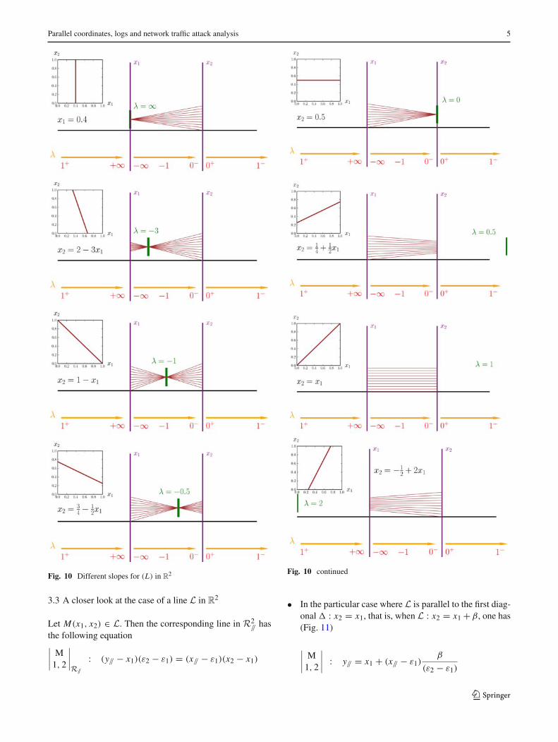
(Fig. 9).The way such a line looks like in //-coordinates mainly

depends on the slope of L.To get an intuitive feeling of what is going on, have a look

at the following plots of L in //-coords for different slopes(Fig. 10):

It seems obvious that in all cases, when M(x1, x2)

describes L, the line

∣∣∣∣M

1, 2

∣∣∣∣ passes by a fixed point who’s

horizontal position solely depends on the slope of L.

123


Fig. 10 Different slopes for (L) in R2

3.3 A closer look at the case of a line L in R2

Let M(x1, x2) ∈ L. Then the corresponding line in R2// has

the following equation∣∣∣∣

M1, 2

∣∣∣∣R//

: (y// − x1)(ε2 − ε1) = (x// − ε1)(x2 − x1)

Fig. 10 continued

• In the particular case where L is parallel to the first diag-onal � : x2 = x1, that is, when L : x2 = x1 + β, one has(Fig. 11)

∣∣∣∣

M1, 2

∣∣∣∣ : y// = x1 + (x// − ε1)

β

(ε2 − ε1)

123


Fig. 11 (L) : x2 = x1 + β

Fig. 12 Random pointson a line L of R

2

meaning that when M describes all of L, the line

∣∣∣∣

M1, 2

∣∣∣∣

remains parallel to vector

(1β

ε2−ε1

)

R//

or

(ε2 − ε1

β

)

R//

.

• In the more general case where L : α1x1 + α2x2 = β isnot parallel to � : x2 = x1, that is, when α1 + α2 �= 0, it

can be easily shown that all lines

∣∣∣∣M

1, 2

∣∣∣∣ have a common

point (Fig. 12).

We will denote that point by

∣∣∣∣

L1, 2

∣∣∣∣, and a straightforward

computation gives∣∣∣∣

L1, 2

∣∣∣∣R//

=(

α1ε1 + α2ε2

α1 + α2,

β

α1 + α2

)

R//

Remark People used to working with projective spaces willimmediately notice that both cases can be described by thepoint

∣∣∣∣L

1, 2

∣∣∣∣R//

= [α1ε1 + α2ε2 : β : α1 + α2]

in RP2.

From now on, we will consider that any line L ⊂ R2 cor-

responds to a point

∣∣∣∣L

1, 2

∣∣∣∣ in R2// and we will not mention

anymore that in some cases that point has to be defined inprojective plane.

Remark Reciprocally, given the point

∣∣∣∣

L1, 2

∣∣∣∣R//

= (x0//,

y0//)R//,

one recovers a cartesian equation of L

L : px1 + (1 − p)x2 = y0//, where p = x0// − ε2

ε1 − ε2

The correspondence between L and

∣∣∣∣L

1, 2

∣∣∣∣ is called by Insel-

berg the line-point duality:

L : α1x1 + α2x2 = β

↓∣∣∣∣

L1, 2

∣∣∣∣R//

= [α1ε1 + α2ε2 : β : α1 + α2]

∣∣∣∣

L1, 2

∣∣∣∣R//

= [x0//, y0//, z0//

]

↓L : (x0// − ε2z0//)x1 + (ε1z0// − x0//)x2 = y0//(ε1 − ε2)

3.4 Vocabulary

The preceding point

∣∣∣∣L

1, 2

∣∣∣∣R//

will be called the level 2

invariant point of line L, or simply the invariant pointof line L, in parallel coordinates.

4 First nontrivial results in //-coordinates

4.1 A first glance at the case of a plane P in R3

As we did for the case of a line L in R2, we will start by some

simple geometrical configuration of an affine plane P in R3.

First of all, we already know that if P is a trivial planexi = β then random points on P show up in R3

// in thefollowing manner (Fig. 13).

In such a case, it is completely obvious that P is entirelycharacterized by the point of convergence of the segments.That point has coordinates (ε1, 1)R//

in our example or, moregenerally, (εi , β)R//

in the case of P : xi = β.We will call that point the invariant point of plane P inparallel coordinates and denote it∣∣∣∣

P1, 2, 3

∣∣∣∣ = [εi : β : 1]

Suppose now that we are in the particular case of P : α1x1 +α2x2 + α3x3 = β where α1 = 0.

We observe that random points on P plot in the followingway (Fig. 14).

In our example of (P) : 0x1 + 2x2 + 3x3 = 7, what hap-pens on the first axis (x1) is uncontrolled since the cartesianequation of P does not involve variable x1. On the other hand,the shortened equation 2x2 + 3x3 = 7 and our initial study

of a line in R2 explain why we observe that all lines

∣∣∣∣

M2, 3

∣∣∣∣

123


Fig. 13 Trivial plane(P) : x1 = 1 in R

3

Fig. 14

(P) : 0x1 + 2x2 + 3x3 = 7

(for M ∈ P) have a common point. We can even computethe (homogeneous) coordinates of that point.

∣∣∣∣

P1, 2, 3

∣∣∣∣ = [2ε2 + 3ε3 : β : 2 + 3]

In the little more general case of P : α2x2 + α3x3 = β theinvariant point would be

∣∣∣∣

P1, 2, 3

∣∣∣∣ = [α2ε2 + α3ε3 : β : α2 + α3]

Now we are going to spend some time with plane P : 2x1 +2x2 + 3x3 = 13 which offers none of the previous partic-ularities. In a certain sense, we can consider it as a randomaffine plane of R

3.If we randomly select some points on it and plot these in

parallel coordinates, we are bound to admit that, this time,no obvious pattern structures the plot (Fig. 15).

But if we intersect P with plane x1 = λ, for differentvalues of λ, we notice some well known patterns! (Fig. 16).

The explanation is easy to give: if x1 is a constant, then x2

and x3 satisfy the equation 2x2 +3x3 = (13−2x1) and that’sthe equation of a line in these two variables. The invariant

point associated with this line has (homogeneous) coordi-nates

[2ε2 + 3ε3 : 13 − 2x1 : 2 + 3]whose abscissae is independent of the constant value of x1.As x1 is fixed to different constant values, the level 2 invari-ant point describes a vertical line (i.e. itself parallel to theaxes of the plot).

This simple observation is going to lead us to the defini-tion of the level 3 invariant point associated to the planeP .

4.2 A closer look at the case of a plane P in R3

Going one step further, we notice that the ordinateβ − α1x1

α2 + α3of the level 2 invariant point of P∩{x1} satisfies, with variablex1, the affine equation

α1x1 + (α2 + α3)(β − α1x1)

(α2 + α3)= β

and in these two variables it is simply the equation of a line.So it should come equipped with an invariant point.

123


Fig. 15 Random points on(P) : 2x1 + 2x2 + 3x3 = 13

Fig. 16 Different intersectionsof (P) : 2x1 + 2x2 + 3x3 = 13with x1 = constant

This is verified on the plot if we draw the lines going fromx1 on the first axis to the corresponding level 2 invariant point.

The point we have constructed using different level 2invariant points will be called the level 3 invariant pointassociated with P (Fig. 17).

As far as it is itself a level 2 invariant point, we can usewhat we know about such points to compute it’s homoge-neous coordinates. We get, after a quick computation

∣∣∣∣

P1, 2, 3

∣∣∣∣ = [α1ε1 + α2ε2 + α3ε3 : β : α1 + α2 + α3]

Now we have to tell whether this point has interesting prop-erties or not and if it is useful to help us decide whethera given point is in P or not.

Remark The previous construction of

∣∣∣∣P

1, 2, 3

∣∣∣∣ is not pos-

sible if α2 + α3 = 0 because of division by zero. Later inthis paper, we will give a different construction of the level3 invariant point, helping us to avoid such accidents.

4.3 A different construction of the level 3 invariant pointof a plane

We study a plane P ⊂ R3 given by

P : α1x1 + α2x2 + α3x3 = β

Let A, B, C be three noncollinear points of P . The plane Pis completely determined by these three points.As we already know, plotting A, B, C in //-coordinates doesnot yield any clear geometric pattern of the kind we had inthe case of a line in R

2 (Fig. 18):What actually happens is that there still is a geometric pat-

tern or geometric organisation in R3// when plotting points

all belonging to a fixed plane P , but it is not as obvious asseen before.

To show this, we will use geometric constructions ofpoints, starting from A, B, C and not the cartesian equation.

Definition Let

∣∣∣∣

AB1, 2

∣∣∣∣ be the unique point of intersection of

the lines

∣∣∣∣

A1, 2

∣∣∣∣ and

∣∣∣∣

B1, 2

∣∣∣∣. This point always exists in the

123


Fig. 17 How level 3 invariantpoint appears for (P) : α1x1 +α2x2 + α3x3 = β

Fig. 18 Three points A, B, C in R3

Fig. 19 Construction of the first level 2 point

projective plane holding R3// even if the two lines are parallel

(Fig. 19).

For such an intersection point, we use the notation

∣∣∣∣AB1, 2

∣∣∣∣ =∣∣∣∣

A1, 2

∣∣∣∣ ·∣∣∣∣

B1, 2

∣∣∣∣

Proposition 1 With all preceding notations we have

Fig. 20 Construction of four level 2 points

∣∣∣∣

AB1, 2

∣∣∣∣R//

= [(b2 − a2)ε1 − (b1 − a1)ε2 : b2a1

− a2b1 : (b2 − b1) − (a2 − a1)]

Of course, in R3//, the same construction can be done with

axes 2 and 3, and with the points B and C . For example,∣∣∣∣

BC2, 3

∣∣∣∣ =∣∣∣∣

B2, 3

∣∣∣∣ ·∣∣∣∣

C2, 3

∣∣∣∣.

If we add these points to the original plot, we obtain (Fig. 20):For the final step of our geometric construction, we need to

draw the line passing by

∣∣∣∣

AB1, 2

∣∣∣∣ and

∣∣∣∣

AB2, 3

∣∣∣∣. We will call this

line

∣∣∣∣

AB1, 2, 3

∣∣∣∣ (Fig. 21):

∣∣∣∣AB

1, 2, 3

∣∣∣∣R//

=(∣∣∣∣

AB1, 2

∣∣∣∣

∣∣∣∣AB2, 3

∣∣∣∣

)

R//

Now let

∣∣∣∣ABC1, 2, 3

∣∣∣∣ (Fig. 22) be defined by

∣∣∣∣ABC1, 2, 3

∣∣∣∣R//

=∣∣∣∣

AB1, 2, 3

∣∣∣∣ ·∣∣∣∣

BC1, 2, 3

∣∣∣∣

123


Fig. 21 Preparing for level 3 point

Fig. 22 Construction of a level 3 point

A simple and remarkable fact is given in the next proposition

Proposition 2 The three lines

∣∣∣∣

AB1, 2, 3

∣∣∣∣ ,

∣∣∣∣

BC1, 2, 3

∣∣∣∣ and

∣∣∣∣

AC1, 2, 3

∣∣∣∣ are convergent. For their common point of inter-

section, we use the following notations:

∣∣∣∣ABC1, 2, 3

∣∣∣∣R//

=∣∣∣∣

AB1, 2, 3

∣∣∣∣ ·∣∣∣∣

BC1, 2, 3

∣∣∣∣ =∣∣∣∣

BC1, 2, 3

∣∣∣∣ ·∣∣∣∣

CA1, 2, 3

∣∣∣∣

=∣∣∣∣

CA1, 2, 3

∣∣∣∣ ·

∣∣∣∣

AB1, 2, 3

∣∣∣∣

This fact can be observed in Fig. 23. The Open Source soft-ware Geogebra4 was used to create an animated constructionand this image.

From the above definition, it is easy to deduce the follow-ing corollary

4 http://www.geogebra.org/.

Corollary 1 Let σ ∈ S({A, B, C}) be any permutation onthe set {A, B, C}. Then,∣∣∣∣

ABC1, 2, 3

∣∣∣∣R//

=∣∣∣∣σ(A)σ (B)σ (C)

1, 2, 3

∣∣∣∣R//

There are many ways to prove the first proposition. For thosenot familiar with projective geometry and Desargues’ the-orem, a direct analytical computation is possible. But if notrick is used to simplify the computation, it might seem hardto do it by hand. In such a case, the open source mathematicalsoftware Sage5 can easily be used to compute the coordinatesof the level three point.

But in the end, it all boils down to a point with quitesimple coordinates: the ones we obtained in our previousconstruction of the level 3 invariant point of P! And that’s afundamental coincidence.

Proposition 3 (Fundamental result)∣∣∣∣

ABC1, 2, 3

∣∣∣∣R//

= [α1ε2 + α2ε2 + α3ε3 : β : α1 + α2 + α3]

in the case where (ABC) is a well defined affine plane withcartesian equation

α1x1 + α2x2 + α3x3 = β

Remark Again, it is visible from the above expression that∣∣∣∣ABC1, 2, 3

∣∣∣∣R//

is invariant under permutation of the letters

A, B, C .

Remark The coordinates of

∣∣∣∣

ABC1, 2, 3

∣∣∣∣R//

only depend on the

coefficients of the cartesian equation of P and of the abscis-sas ε1, ε2, ε3 used when building R3

//.

This motivates the following definition.

Definition Let P : α1x1 + α2x2 + α3x3 = β be a plane ofR

3.We define the level 3 point invariant of P in R3

// as the point∣∣∣∣

P1, 2, 3

∣∣∣∣R//

= [α1ε2 + α2ε2 + α3ε3 : β : α1 + α2 + α3]

Remark It is very important to understand that P completelydetermines∣∣∣∣

P1, 2, 3

∣∣∣∣R//

but the reciprocal is false.

Obviously, the knowledge of

∣∣∣∣P

1, 2, 3

∣∣∣∣R//

is not enough to

recover the original cartesian equation of P . At least, youneed the data of a point A in P .

It can be shown that it is then enough to recover P .

5 http://www.sagemath.org.

123

http://www.geogebra.org/

http://www.sagemath.org


Fig. 23 Constructions of level two and level three points for (ABC)

5 Geometrical proof of Proposition 2

We will begin with a short review of projective geometry.

5.1 A quick introduction to projective geometry

Projective geometry only considers points and lines and doesnot use notions as distance or angle. It is based (classically)on 4 axioms:

• By two points, there always is a line passing, which isunique if the two points are different

• Two lines always meet• It is possible to find 4 points such that any three of them

are never aligned• Pappus’ theorem

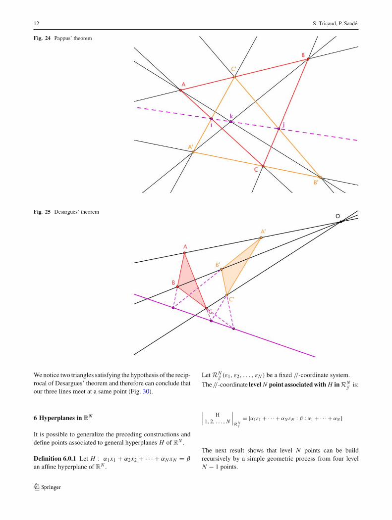
Pappus’ theorem has many different expressions but an easyone can be read from the following figureLet (ABC) and (A′ B ′C ′) be two triangles such that C ∈(A′ B ′) and C ′ ∈ (AB).Let i = (AC) ∩ (A′C ′), j = (BC) ∩ (B ′C ′) and k =(AB ′) ∩ (A′ B).Then i, j, k are aligned.One of the first consequence of Pappus’ theorem is the famousDesargues’ theorem.Consider the following figure (Figs. 24, 25)

Desargues theorem states that if (ABC) and (A′B ′C ′) aretwo triangles such that (AA′), (B B ′) and (CC ′) meet in acommon point O , then the points of intersection of sides ofboth triangles having same names are aligned.More precisely, if i = (AB)∩ (A′ B ′), j = (AC)∩ (A′C ′),k = (BC) ∩ (B ′C ′), then i, j, k are on a same line.

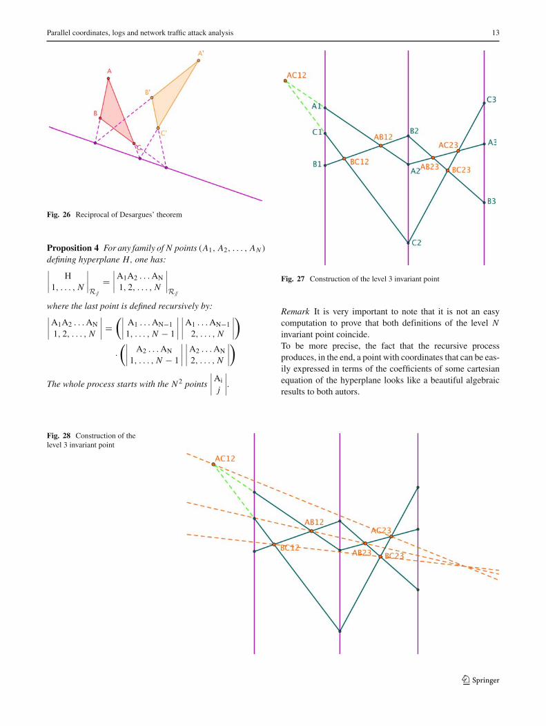
By a very important duality principle in ProjectiveGeometry, Desargues’ theorem admits a reciprocal. Thisreciprocal states that, with the preceding notations, if i, j, kare aligned then (AA′), (B B ′) and (CC ′) meet in a commonpoint (Fig. 26).

Using this result, it is possible to prove the first propositionconcerning the level 3 invariant point.

5.2 A geometrical proof of Proposition 2

Recall that our geometric construction of

∣∣∣∣

ABC1, 2, 3

∣∣∣∣ is based

on the following process.We first compute the six points obtained by intersecting linesin-between the same axes (Fig. 27).

Then, we pretend that the three lines

∣∣∣∣AB

1, 2, 3

∣∣∣∣ ,∣∣∣∣

BC1, 2, 3

∣∣∣∣ and∣∣∣∣

AC1, 2, 3

∣∣∣∣ are convergent (Fig. 28).

To prove this, we will simplify the drawing and only keepthe central axis (Fig. 29)

123


Fig. 24 Pappus’ theorem

Fig. 25 Desargues’ theorem

We notice two triangles satisfying the hypothesis of the recip-rocal of Desargues’ theorem and therefore can conclude thatour three lines meet at a same point (Fig. 30).

6 Hyperplanes in RN

It is possible to generalize the preceding constructions anddefine points associated to general hyperplanes H of R

N .

Definition 6.0.1 Let H : α1x1 + α2x2 + · · · + αN xN = β

an affine hyperplane of RN .

Let RN// (ε1, ε2, . . . , εN ) be a fixed //-coordinate system.

The //-coordinate level N point associated with H in RN// is:

∣∣∣∣

H1, 2, . . . , N

∣∣∣∣RN

//

= [α1ε1 + · · · + αN εN : β : α1 + · · · + αN ]

The next result shows that level N points can be buildrecursively by a simple geometric process from four levelN − 1 points.

123


Fig. 26 Reciprocal of Desargues’ theorem

Proposition 4 For any family of N points (A1, A2, . . . , AN )

defining hyperplane H, one has:∣∣∣∣

H1, . . . , N

∣∣∣∣R//

=∣∣∣∣A1A2 . . . AN

1, 2, . . . , N

∣∣∣∣R//

where the last point is defined recursively by:∣∣∣∣A1A2 . . . AN

1, 2, . . . , N

∣∣∣∣ =

(∣∣∣∣

A1 . . . AN−1

1, . . . , N − 1

∣∣∣∣

∣∣∣∣A1 . . . AN−1

2, . . . , N

∣∣∣∣

)

·(∣

∣∣∣A2 . . . AN

1, . . . , N − 1

∣∣∣∣

∣∣∣∣A2 . . . AN

2, . . . , N

∣∣∣∣

)

The whole process starts with the N 2 points

∣∣∣∣Ai

j

∣∣∣∣.

Fig. 27 Construction of the level 3 invariant point

Remark It is very important to note that it is not an easycomputation to prove that both definitions of the level Ninvariant point coincide.To be more precise, the fact that the recursive processproduces, in the end, a point with coordinates that can be eas-ily expressed in terms of the coefficients of some cartesianequation of the hyperplane looks like a beautiful algebraicresults to both autors.

Fig. 28 Construction of thelevel 3 invariant point

123


Fig. 29 Simplifying the figure

7 Detection of more general geometric structureswith //-coords

As we want to keep this mathematical introduction quiteelementary, our journey in the theoretical //-coords universewill stop shortly. We hope that the very basic aspects of //-coords are now familiar to you and that you understand betterhow classical affine geometric objects can be detected.

Of course, we know that it is not enough to detect linearstructures and that in real life, the mathematical relationshipbetween variables can be more complex. It is therefore essen-tial to know wether //-coordinates are able or not to deal withsuch datasets.

Furthermore, it is one thing to examine a puremathematical object defined by a set of algebraic equations inR

N (as in real algebraic geometry), and it is another to man-age experimental data that are supposed to obey a certainclass of mathematical laws. It is even a third story to investi-gate computer security logs given that it is very doubtful thatany analytical relationship exists between the variables.

In a forthcoming article, we hope to report about a classi-fier based on //-coords and pioneer work of Inselberg [6–9]and some new ideas. This classifier, hopefully, will show how//-coords can go much beyond our actual exposition.

8 Automating //-coords creation with Picviz

Now that the theory behind //-coords is known, and sincePicviz goal is to automate the creation of //-coords imagesout of logs, this section introduces its architecture and howit can be used to discover security issues. Picviz is not lim-ited to computer security, however since it is a good goal todemonstrate how powerful can be such a tool, this is whatthe paper sticks to.

Because digging visually for security issues is aimed tobe very practical, Picviz presentation starts with an authen-tication log investigation. After this short presentation, thearchitecture is detailed. Once the reader knows features pro-vided by the software, two examples are given.

Fig. 30 How we apply thereciprocal of Desargues’theorem

123


8.1 Picviz

Picviz6 is a software transforming acquired data into aparallel coordinates plot image to visualize data and discoverinteresting results quickly. Picviz is composed in three parts,each facilitating the creation, tuning and interaction of //-coords graphs (Fig. 31):

• Data acquisition: log parsers and enricher• Console program: transforms PGDL into a svg or png

image. Unlike the graphical frontend, it does not requiregraphical canvas to display the lines, it is fast and able togenerate millions of lines.

• Graphical frontend: transforms PGDL into a graphicalcanvas for user interaction.

It was written because of a lack of visualization tools ableto work with a large set of data. Graphviz is very close tohow Picviz works, except that is has limitations regardingthe number of dimensions that can be handled by a directedgraph, such as when dealing with time.

8.2 Data acquisition

The data acquisition process aims to transform captured logsinto the Picviz Graph Description Language (PGDL) filebefore Picviz treatment. In this paper, log is used interchange-ably with data to express something that is captured from oneor several machines. That being one in:

• Syslog: System and application log files. Containing atleast four variables: time, machine, application and thelogged event.

• Network: Sniffed data.• Database: Structured information storage.• Specific: Log file for applications not using standard log

functions.• Other: Any other way to record events.

CSV being a common format to read and write such data,Picviz can take it as input and will translate it into PGDL.

8.3 Console program

The Command Line Interface (CLI) allows Picviz to easilygenerate //-coords graphs, including frequency analysis, fil-tering and powerful filters. As the CLI allows to deal withmillions of events, this may be the first step prior using thegraphical frontend. The CLI is the pcv program that is beingused in this paper to show how graphs were generated.

6 This paper describes Picviz version 0.6.x.

8.4 Graphical frontend

While the Graphical frontend does not allow to deal with asmuch objects as the CLI does, it still gives valuable insightfor the analyst. Live interaction is something the frontendcan provide:

• moving the mouse over the lines will actually show thelines values being displayed,

• changing the axis order on the fly by selecting the appro-priate value on the axis description box,

• zooming to allow line-to-line relationship finding(Fig. 32),

• slider to move in the event time scale: moving the cursorto the left-most will show the first event,

• brushing to find the relationships in multiple dimensionsof a given event (Fig. 33).

8.5 Understanding 10000 lines of log

Visualization is an answer to analyze a massive amount oflines of logs. //-coords helps to organize them and see cor-relations and issues by looking at the generated graph [3].

Each axis strictly defines a variable: logs, even those thatare unorganized, are always composed by a set of variables.At least they are: time when the event occurred, machinewhere the log comes from, service providing the log infor-mation, facility to get the type of program that logged, andthe log itself.

The log variable is a string that varies widely based on theapplication writing it and what it is trying to convey. Thisvariability of the string is what makes the logs disorganized.From this string, other variables can be extracted: username,IP address, failure or success, etc.

Log sample: PAM session

Aug 11 13:05:46 quinificated su[789]:pam_unix(su:session): session openedfor user root by toady(uid=0)

Looking at the PAM session log, we know how the userauthenticates with the common pam_unix module. We knowthat the command su was used by the user toady to authenti-cate as root on the machine quinificated on August 11th at1:05 p.m.. This is useful information to care about whendealing with computer security. In this graph we clearlyidentify:

• If a user sometime fails to give the correct password• If a user logged in using a noncommon pam module or

service• Time when users log in

123


Fig. 31 Picviz simplified architecture

Fig. 32 Graphical frontend zoom feature

Fig. 33 Graphical frontend brushing feature

Figure 34 shows the representation of the auth syslogfacility:

AnalysisWhat one can easily see in Fig. 34 is how many users

logged in as root on the machine: red lines means root des-tination user. Also, the leftmost axis (time) is interesting: ithas a blank area and using the frontend we discover that noone opened a session between 2:29 a.m. and 5:50 a.m.:

The second axis is the machine where the logs origi-nated. Since this example is a single machine analysis, linesconverge to a single point.

Fig. 34 Picviz frontend showing pam sessions opening

Fig. 35 Zoom on time axis

Fig. 36 PAM module convergence

This third axis is the service or application that wrote thelog. We can quickly see four services (one red, three blacks,the line at the bottom is also a connection between two axes):moving the mouse above the red line at the service on top ofFig. 35 shows that only the ’su’ service is used to log a useras root. Hopefully no one logs in using gdm, kdm or loginas root.

The fourth axis is the pam module that was used toperform the login authentication: again, as only local authen-tication was done using the pam_unix module, lines are con-verging. If we would have had a remote authentication, orother modules opening the session, we would see them onthis axis (Fig. 36).

The fifth and sixth axis are the user source and destinationof the logs. We have as much source logins as destination lo-gins. On this machines, logins are both su and ssh.

As experts might know, //-coords are already used incomputer security [1] but face a problem of not being easy toautomate or with various data formats. This paper focuses onhow relevant security information can be extracted from logs,whatever format they have, how anyone can discover attacks

123


or software malfunctions and how the analyst can then filterand dig into data to discover high level issues. The next partcovers how Picviz was designed, its internals. After we willsee how malicious attacks can be extracted, and how it canhelp you to write correlation rules.

9 Picviz architecture in detail

9.1 Picviz graph description language

It has been designed to be easy to generate and as close aspossible to the Graphviz [2] language (mostly for proper-ties names). It is a description language for //-coords whichallows to specify all kinds of properties for a given line(data), set each axis variable axes and give instructions tothe engine in the engine section. Also, a graph title can beset in the header section.

Below is an example of a PGDL source which representsa single line:

header {title = "foobar";}axes {integer axis1 [label="First"];string axis2 [label="Second"];}data {x1="123",x2="foobar" [color="red"];}

Despite CSV being a standard for log normalization inorder to create a graph, and even though Piviz can convertCSV into PGDL, CSV is not recommended. It is impossibleto set properties on an individual line when a specific itemis encountered. This would require an external configurationfile to be parsed at every new added line. This would greatlydecrease performances. Also, //-coords have the weakness ofhiding interesting values according to the axis order. Chang-ing the axis order in PGDL is as simple as moving a line inthe axes section.

9.1.1 The axes section

It defines possible types you can set to each axis, as wellas setting axis properties. Labels can be set to axes with thelabel property. Axes types must be one of them:

Type Range Descriptiontimeline "00:00" - "23:59" 24 h timeyears "1970-01-01 00:00"

-Several years

"2023-12-31 23:59"integer 0 - 65535 Integer numberstring "" - "No specific A string

limit"short 0 - 32767 Short numberipv4 0.0.0.0 - IP address

255.255.255.255gold 0 - 1433 Small valuechar 0 - 255 Tiny valueenum anything Enumerationln 0 - 65535 Log(n) functionport 0 - 65535 Special way to

display portnumbers

It is indeed possible to specify the maximum value anaxis can get as a numeric value instead of the axis type. Thiswould allow value 1234 to be the maximum of axis1:

axes {1234 axis1;...

}

Other available properties are:

• print: when set to false, removes values printing on lines.It is usually used when an axis had too big values whichare overlapping the next axis.

• relative: when set to true place values on the axis rela-tively to each other. Which decreases performances butcan improve the axis reading.

9.1.2 The data section

Data are written line by line, each value coma separated. Fourdata entries with their relatives axes can be written like this:data {t="11:30",src="192.168.0.42", dport="80"[color="red"];

t="11:33",src="10.0.0.1", dport="445";t="11:35",src="127.0.0.1", dport="22";t="23:12",src="213.186.33.19", dport="31337";}

The key=value pair allows to identify which axis has whichvalue. Since axis variable type was defined in the previousaxis section, the order does not matter. For the previous data,if one want to respect the order, the axis section would be:

axes {timeline t;ipv4 src;port dport;

}

123


Changing the axis order and repeating the axes is explainedin the Grand tour section.

Every line can receive two properties: color and pen-width, which allow to set the line color and width, respec-tively.

Data lines are generated by scripts from various sources,ranging from logs to network data or anything a script cancapture and transform into PGDL language data section.This paper focuses on logs, and Perl was chosen for its con-venience with Perl compatible regular expressions (PCRE)built-in with the language. The next part explains how sucha script can be written to generated the PGDL.

9.2 Generating the language

Picviz delivers a set of tools to automate the PGDL generationfrom various sources, such as apache logs, iptables logs,tcpdump, syslog, SSH connections, …Perl being suited language for this kind of task, it was chosenas the default generator language. Of course, nothing preventother people to write generators for their favorite language.

The PGDL is generated with the Perl print function, alongwith Perl pattern matching capabilities to write the data sec-tion. The syslog to PCV takes 25 lines of code, includinglines colorization where the word ’segfault’ shows up in thelog file. Then, to use the generator, type:

perl syslog2pcv /var/log/syslog > syslog.pgdl

To help finding evilness, a Picviz::Dshield class was writ-ten. Calling it will check if the port or IP address match withdshield.org database:

use Picviz::Dshield;

dshield = Picviz::Dshield->new;

ret = dshield->ip_check("10.0.0.1")

It can be used to set the line color, to help seeing an eventcorrelated with dshield information database.

9.3 Understand the graph

9.3.1 Graphical frontend

Aside from having a good looking graph, it is good to dig intoit, and see what was generated. An interactive frontend waswritten for this purpose. It is even a good example on howPicviz library can be embeded in a Python application. Theapplication picviz-gui was written in Python and TrolltechQT4 library.

The frontend provides a skillful interaction to findrelationship among variables, allows to apply filters, dragthe mouse over the lines to see the information displayed

and to see the time progression of plotted events. Real-timecapabilities are also possible, since the frontend listen to asocket waiting for lines to be written.

The frontend has limitations: on a regular machine, morethan 10000 events makes the interface sluggish. As Picvizwas designed to deal with million of events, a console pro-gram was written.

9.3.2 Command line interface

The pcv program is the CLI binary that takes PGDL as input,uses the picviz library output plugins and generate the graphusing called plugin. To generate a SVG, the program can becalled like this:

pcv -Tsvg syslog.pgdl > syslog.svg

As SVG is a XML and vectorial format, it will performwell when a few thousand of line are drawn: the operator willbe able to do actions on items, select them, grep for a certainvalue, move the lines, etc.

However, with a big set of data, SVG frontend will faildoing the rendering.

This is why a PNG capable plugin was written. Using thecairo7 library. The plugin is named ‘pngcairo’ and can beused like this:

pcv -Tpngcairo syslog.pgdl > syslog.png

Usually is it better to use the PNG plugin, filter data and ifneeded, use then choose between the SVG plugin to use all thefeatures a vectorial image can provide or the Picviz frontend,that is designed to deal with //-coords issues. Section 2.3.4explains how filters can be used with Picviz.

9.3.3 Grand tour

Because choosing the right order for the right axis is one of//-coords disadvantages, Picviz provides via the pngcairoplugin a Grand tour capability. The Grand tour generatesas much images as pairs permutation of axes possible, theidea is to show every possible relation among every availableaxes. Plugin arguments are provided with the -A command.So to generate a grand tour on graphs, pcv should be calledlike this (Fig. 37):

pcv -Tpngcairo syslog.pcv -Agrandtour...File Time-Machine.png writtenFile Time-Service.png written...File Log-Machine.png writtenFile Log-Service.png written

7 http://www.cairographics.org.

123

http://www.cairographics.org


Fig. 37 Syslog grand tour

An other way to change the axes order is simply changingtheir order in the axes section.

axes {integer axis1;string axis2;ipv4 axis3;}

Shows in the order: axis1, axis2 and axis3, while:

axes {ipv4 axis3;integer axis1;string axis2;ipv4 axis3;}

will show the axes in the order axis3, axis1, axis2 and thenaxis3 again. Thus changing the axes–pair relationship. Thissection also allows commenting to hide a given axis.

It is recommended to have the data separated from theimage and axes properties to allow easy changing, this canbe done using the @include keyword, that will include datafrom a third-party file. In the case of numerous data, this isvery convenient to find relationships and allow easy changingof axis type and order:

axes {ipv4 axis3;integer axis1;string axis2;}data {

@include "mydata.pgdl"}

9.3.4 Real-time

Picviz can be set up to perform real-time line drawing bylistening to a socket. Then programs can send their lines tothis socket.

When Picviz listen to a socket, it should have a templateassociated with it. This is a graph written in a template derivedfrom PGDL named PGDT for Picviz Graph Description Tem-plate. The difference with a PGDL file is that a template maynot have any data, so that the program will know which vari-ables are associated with the axes. Of course PGDT is moreconvenient to express a file that is created for real-time, butit can interchangeably be used with PGDL.

To start PCV in real-time mode, one can start on one side:

pcv -s local.sock -t samples/test1.pgdl-Tpngcairo -o /tmp/graph.png

And on the other side, the client will simply need to writeonto this socket:

echo "t=\"12:00\", i=\"100\",s=\"I write some stuff\";"

The OSSEC HIDS8 can output its alerts to Picviz, usingthe template ossec.pgdt provided with sources.

9.3.5 Filtering

To select lines one want to be displayed, Picviz providesfilters. They can be used on the real value to match a givenregular expression, line frequency, line color or position asmapped on the axis. It is a multi-criterion filter. It is set withthe CLI or Frontend parameters.

With the CLI, they can be called like this:

pcv -Tpngcairo syslog.pcv ’your filter here’

With the frontend, filter can be called like this:

picviz-gui syslog.pcv ’your filter here’

Filter syntax is:

display type relation value on axisnumber && ...

Where:

• display: show or hide, select if we hide or display theselected value

• type: value, plot, color or freq, choose what is filtered• relation: <, >, <=, >=, ! =, =, relation with selected

value

8 http://www.ossec.net.

123

http://www.ossec.net


Fig. 38 SSH scan

• value: selected value to compare data with• on axis: text to express the axis selection• number: axis number to filter values on

For example, to display all lines plotted under a hundredon the second axis, one can replace your filter here by plot< 100 on axis 2. Specific data can also be removed, such as:

pcv -Tpngcairo syslog.pcv ’value = "sudo"on axis 2’

A percentage can be applied to avoid knowing the valuethat can be filtered: ‘plot >(42% on axis 3 and plot < 20%on axis 1’.

9.3.6 String positioning

One of the basic string algorithm displaying is to simply addthe ascii code to create a number. Among pros of using thisvery naive algorithm, is to be able to display scans (stringsvery close to each other coming from one source) very easily.As for the cons there is the collision risk, but in practice thislow risk of having such events. As Picviz is very flexible, itstill offer other string alignment algorithms, using Levenstein[10] or Hamming distance [4] from a reference string. Thisstill makes collision possible, but differently.

The basic algorithm highlights scans evidences, and thenone can quickly spot an issue. This way, without having anyknowledge of how the log must be read, little changes willappear close enough to each other to grab the reader attention.

The following lines are logs taken from ssh authentication,and appear like this:

time="05:08", source="192.168.0.42",log="Failed \ keyboard-interactive/pamfor invalid user lindsey";time="05:08", source="192.168.0.42",log="Failed \ keyboard-interactive/pam

Fig. 39 Same shared value

Fig. 40 Syslog heatline with virus mode

for invalid user ashlyn";time="05:08", source="192.168.0.42",log="Failed \ keyboard-interactive/pamfor invalid user carly";

Figure 38 shows a generated graph from twenty lines of assh scan.

On the third axis, one can clearly see the lines sweep,showing the scan.

9.3.7 Correlations

With //-coords, several correlations are possible, as shown inFig. 39, where it is known for sure all events share a commonvariable.

One other way to correlate is applying a line colorizationfor their frequency of apparition between two axes and col-orize the whole line, according to the highest value. Picvizcan generate graphs in this mode with the heatline renderingplugin and its virus mode (Fig. 40).

123


Fig. 41 Picviz curves

As of today, only the svg and pngcairo handle this feature.Picviz CLI should be called like this:

pcv -Tpngcairo syslog.pgdl -Rheatline-Avirus > syslog.png

9.3.8 Curves

Curves is the idea of drawing arc circles instead of lines tomaybe uncover clusters more easily. While this techniquewill go against all the mathematical theory described in thispaper, some people consider this. Nothing useful has beenfound using this technique. It is shown to get an idea of whatone can do with //-coords. See Fig. 41.

9.3.9 Section summary

Picviz has been designed to be very flexible and let anyonecapable to generate the language, filter data and visualizethem. This can be done statically on a plain generated file, andwith the graphical interface, this is even possible in real-time.Of course the knowledge of logs lines is better to set more axisand have more information to understand the graph. How-ever, the naive approach is sometime enough to see scanningactivities.Now that the Picviz architecture and features have beenexplained, we will show how we can efficiently use it todig into logs and extract relevant information.

The next section covers how we can efficiently see attacksfrom many lines of log and finally write a correlation scriptin perl.

10 Understanding the unknown

This section explains how one can handle in a very shortamount of time the analysis of failures a system can have

based on their logs. The log issues coverage will not beexhaustive but using //-coords can easily spot some.

During the latest Usenix Workshop on the Analysis ofSystem Logs 2008, Cray systems gave logs to analysts to seewhat they could extract from them.

Cray logs are available for download in the Usenix web-site. 9 This analysis is done on the file 0809181018.tar.gz.

10.1 Files overview

Once uncompressed, there are sixty-seven files and four maindirectories, which are:

• eventlogs• log• SEDC_FILES• xt

The log directory does not contain enough information: asingle 18 lines file. As Picviz is good to manage big files, theeventlogs directory was chosen.

The eventlogs directory has two files: eventlogs andfiltered-eventlog. As the last file is smaller and from its nameseems to be filtered, it is best to run Picviz on eventlogs.

10.2 Dissecting the eventlogs file

The eventlog file looks like:

2008-09-18 04:04:54|2008-09-1804:04:54|ec_console_log| \ src:::c0-0c0s3n0|svc:::c0-0c0s3n0|

2008-09-18 04:04:54|2008-09-18 04:04:54|ec_console_log| \src:::c0-0c0s3n0|svc:::c0-0c0s3n0|7[?25l[1A[80C[10D[1;32mdone[m8[?25h

2008-09-18 04:04:54|2008-09-1804:04:54|ec_console_log| \

9 http://cfdr.usenix.org/data.html#cray.

123

http://cfdr.usenix.org/data.html#cray


Fig. 42 Cray eventlogs graph

src:::c0-0c0s3n0|svc:::c0-0c0s3n0|cat:/sys/class/net/rsip333x1/type

2008-09-18 04:04:54|2008-09-18 04:04:54|ec_console_log| \src:::c0-0c0s3n0|svc:::c0-0c0s3n0|:No such file or directory

By looking through this log file one may discern five fields:

• 2008-09-18 04:04:54|2008-09-18 04:04:54: time value,because of the lack of knowledge of Cray logs for whythere are two identical timestamps, the first is taken. Thevariable timeline should be appropriate.

• ec_console_log: unknown value, which seems like anenumeration of a few possible items. It looks like an eventcategory. The variable enum should be appropriate.

• src:::c0-0c0s3n0: should be the source node where theeven come from. Again, since there are a limited num-ber of distinct resources, the variable enum should beappropriate.

• svc:::c0-0c0s3n0: should be the destination. Just like forsources, the enum variable should be appropriate.

• : No such file or directory: is the log itself. The stringvariable is appropriate and will be put as relative withthe other strings.

Below the perl code for the generator to handle Cray eventslog file:

print "axes {\n";print " timeline t [label=\"Time\"];\n";print " enum e [label=\"Event\"];\n";print " enum s [label=\"Src\"];\n";print " enum d [label=\"Svc\"];\n";print " string l [label=\"Log\",relative=\"true\"];\n";

print "}\n";

10.3 Graphing

From the PGDL source generated and using the axes pairfrequency rendering, a graph is created in Fig. 42.

//-coords reveals the following facts:

• Time range: logs were written in a very short at veryspecific time. Without being accurate, one can say alllogs are written between about 5 a.m. and 11 a.m.

• Coverage: one event (the one in the middle) covers allsources.

• Frequency: the red lines shows that one event occursway more than the other, that there is a source-destinationtriggering most of the events and a log occurs more thanthe others.

• Differentiation: Some low-frequency logs are far awayfrom all the other logs. Interesting.

10.4 Filtering

As it is usually interesting to start with those events thatappear in low frequency on top of the fifth axis, a filtering isapplied:

pcv -Tpngcairo event.pcv ’showplot > 90% on axis 5’ -a

Which gives the Fig. 43.No need for frequency analysis here, since it was done

in the first graph. This graph outlines that a very few logswere written, that they all come from the same class of event(second axis) and a few machines among all that were in thefirst graph make them.

Logs generating those lines are:

123


Fig. 43 Cray filtered eventlogs graph

10.4.1 Log #1

Bootdata ok (command line is earlyprintk=rcal0 load_ramdisk=1

ramdisk_size=80000 console=ttyL0bootnodeip=192.168.0.1 bootproto=ssip

bootpath=/rr/current rootfs=nfs-sharedroot=/dev/sda1 pci=lastbus=3

oops=panic elevator=noop xtrel=2.1.33HD)

Interesting keywords: earlyprintk, oops=panic.

10.4.2 Log #2

Bootdata ok (command line is earlyprintk=rcal0 load_ramdisk=1 CMD LINE[earlyprintk=rcal0 load_ramdisk=1ramdisk_size=80000 console=ttyL0bootnodeip=192.168.0.1 bootproto=ssipbootpath=/rr/currentrootfs=nfs-shared root=/dev/sda1pci=lastbus=3 oops=panic elevator=noopxtrel=2.1.33HD]

Interesting keywords: earlyprintk x2, CMD LINE,oops=panic.

10.4.3 Log #3

Bootdata ok (command line is earlyprintk=rcal0 load_ramdisk=1 Kernel

command line: earlyprintk=rcal0load_ramdisk=1 ramdisk_size=80000

console=ttyL0 bootnodeip=192.168.0.1bootproto=ssip bootpath=/rr/current

rootfs=nfs-shared root=/dev/sda1pci=lastbus=3 oops=panic elevator=noop

xtrel=2.1.33HD

Interesting keywords: earlyprintk x2, Kernel commandline, oops=panic.

10.4.4 Log #4

Lustre: garIBlus-OST0005-osc-ffff8103f3fab800: Connection to service

garIBlus-OST0005 via nid 19@ptl waslost; in progress operations using this

service will wait for recoveryto complete.

Interesting keywords: Connection to service … was lost,wait for recovery to complete.

As one can see, Picviz successfully help to trace eventson the most used node based on both frequency analysis andhigh values on the log axis. Because printk are the Linuxkernel print function handling anything the kernel wants toprint in usual abnormal situations, it is worth taking a lookat it.

pcv -Tpngcairo -Wpcre event.pcv ’showvalue = ".*printk.*" on axis 5 -a

Which gives the Fig. 44, which outlines on the fifth axislines previously seen, and others, appearing at about 10%on the same axis, that were mixed with the other logs. Bylooking at those logs value, there is:

10.4.5 Log #1

printk: 64 messages suppressed

10.4.6 Log #2

printk: 336 messages suppressed

123


Fig. 44 Cray eventlogs graph with printk

Which reveals a set of repeated problems.Of course, knowing exactly what occurred would require

more work and knowledge of Cray systems. However using//-coords helped to understand easily what was happeningon those machines, the way they log, the number of sourcesand what seems to be destinations.

In this section, the way //-coords were used may be lookedas if one would have use the grep tool. Actually, the firstgenerated picture and its frequency analysis helped to targetdata that could be most likely the source of an issue. Then,because lines were drawn far away from all the other and inlow frequency, it went fairly easy to spot and focus on theprintk.

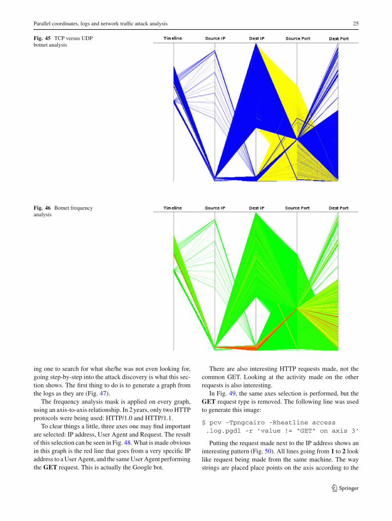
11 Botnet analysis

Botnets attacks consists of spreading a malware to usuallyvulnerable Windows systems to get a maximum of machines.This big amount of machines allows an attacker to spreadspams and make denial of services (DoS) attacks. Botnetscan be controlled from IRC commands or similar customprotocol. Also files can be sent through various nodes usinga peer to peer protocol [5].

When facing a Botnet attack, one will see connectionsfrom a big load of different source IP addresses. Making ithard to block. Most of the time, empirical tricks are beingused to kill an ongoing DoS attack, such as renaming thetarget web file, etc.

This section does not intend to explain details of a botnetattack, but how such an attack looks like and how it can beunderstood to help defending against it.

Because Picviz is good with such a number of events, aBotnet attack was captured and Argus was used to clear outnetwork flows, it was used to generate a //-coords graph.

In this example, two types of images based on the samedata were generated. Only the color varies:

• Figure 45: UDP traffic is in blue, TCP traffic in yellow• Figure 46: Frequency analysis per pair-axes wise

Based on those two figures, it is easy to outline:

• The attack happens on two times: the first starting at about1 p.m. and stopping 30 min after. The second attack isbigger: starting at about 2 p.m. and stopping 3 h latter.

• The TCP flow starts during the second attack and lastduring a short period of time.

• The frequency analysis is more interesting: one can eas-ily see that several IP addresses knocked the same sourceport. Also, one single source IP receives most of the traf-fic. This is because it is the target machine.

• When superposing the two pictures, most of the generatedtraffic happens at the same time TCP traffic happens.

As an emergency counter-measure, two solutions can beconsidered: blocking any UDP traffic that is not DNSrequests, NTP traffic or any critical service required by thenetwork. Also, since the source port is shared for most ofIP sources, it seems this value was hardcoded. Blocking thisspecific port may help resolving the problem for the time theadministrator can take to understand more about the attack.

In all, even though the botnet understanding requires sometime, using //-coords to see obvious facts can help havingmore time to investigate deeper.

12 Apache access.log analysis

Trying to find evil requests within 2 years, the first thing onemay do is to use known-patterns against the log. Picviz allow-

123


Fig. 45 TCP versus UDPbotnet analysis

Fig. 46 Botnet frequencyanalysis

ing one to search for what she/he was not even looking for,going step-by-step into the attack discovery is what this sec-tion shows. The first thing to do is to generate a graph fromthe logs as they are (Fig. 47).

The frequency analysis mask is applied on every graph,using an axis-to-axis relationship. In 2 years, only two HTTPprotocols were being used: HTTP/1.0 and HTTP/1.1.

To clear things a little, three axes one may find importantare selected: IP address, User Agent and Request. The resultof this selection can be seen in Fig. 48. What is made obviousin this graph is the red line that goes from a very specific IPaddress to a User Agent, and the same User Agent performingthe GET request. This is actually the Google bot.

There are also interesting HTTP requests made, not thecommon GET. Looking at the activity made on the otherrequests is also interesting.

In Fig. 49, the same axes selection is performed, but theGET request type is removed. The following line was usedto generate this image:

$ pcv -Tpngcairo -Rheatline access.log.pgdl -r ’value != "GET" on axis 3’

Putting the request made next to the IP address shows aninteresting pattern (Fig. 50). All lines going from 1 to 2 looklike request being made from the same machine. The waystrings are placed place points on the axis according to the

123


Fig. 47 First full access.log

Fig. 48 Axes selection inaccess.log

string length. This shows requests that are bigger and bigger.Indeed, this is a Google bot fetching any available pages. Thered line shows that this is event occurs frequently, show howa bot can be active (Fig. 51).

Picviz can also filter on events frequency, this allows sortevents regarding how frequent they appear (filtering with‘freq < 0.0005’).

13 WLAN images

Current technology involves Wireless when connecting tothe internet. While this paper does not intend to explain WEP

cracking such as in [11], the two images in Figs. 52 and 53show some obvious patterns: one looks like normal, and theother looks like there is some sort of broadcast happening.

While understanding the attack requires how WEP crack-ing happens, several kind of people can deal with this prob-lem: administrators can give the picture to analyst, who willthen look for the relationships and tag the source emittingthe broadcast.

What the Fig. 53 shows is the initialization phase of WEPcracking

Even though it is fairly easy to write a simple script able todetect the broadcast, the visualization and the multi-dimen-

123


Fig. 49 Axes selection inaccess.log

Fig. 50 Pattern in access.log

Fig. 51 Low frequency eventsfrom access.log

123


Fig. 52 WLAN without any attack

Fig. 53 WLAN initialization vector generated on the fly before a WEP key cracking

sion aspect of //-coords allows to spot what looks obvious,but would not have been without using this technique.

14 Conclusion

This paper explained a disruptive way of responding to com-puter security related events using //-coords. This was exclu-sively run from system logs and network traffic. It can ofcourse be extended to other parts of a machine, such as sys-tem calls or application behavior.

However, this paper neither covered all theoretical aspectsnor all practical usage of //-coordinates. Much remains to bedone, proved and experienced in both directions.

First of all, on the theoretical background:

• one should decide whether //-coordinates are efficient ornot in analysing randomly generated points of mathe-matically well defined object.

• one should precisely explain how and why //-coordinatescan be of any interest on datasets not coming from anymathematical definition (such as one encounters in com-puter security).

On the practical background of computer security, weproved how efficient //-coordinates images can be to helpsecurity administrators to find rare and unexpected events,as much as understand more complex mechanisms hidden inhuge amounts of information.

We hope to investigate soon on the two questions aboveand report clear explanations (more or less based on somealready existing literature).

Picviz offers a very efficient tool to get a quick and faith-ful look into gathered datasets: frequency is taken intoaccount (axis by axis or on all axes together), offering atransversal information correlation which proved not to beobvious.

123


The generated image can be very technical and has itslearning curve to be able to tune and help to get an efficientimage one can easily find things in. However, even whenreacting as a naive person, generating a picture a day cankeep the doctor away and help to discover tendencies beforeit is too late. The kind of images Picviz can generate can beread by several kind of people and thus improves the networksecurity reaction at several layers.

The future of Picviz will be to automate visually correla-tions and go further than //-coords to make a better represen-tation of axes correlations.

References

1. Conti, G., Abdullah, K.: Passive visual fingerprinting of networkattack tools. In: VizSEC/DMSEC ’04: Proceedings of the 2004ACM Workshop on Visualization and Data Mining for ComputerSecurity, pp. 45–54. ACM, New York, NY, USA (2004)

2. Gansner, E.R., Koutsofios, E., North, S.C., Phong Vo, K.: Atechnique for drawing directed graphs. IEEE Trans. Softw.Eng. 19, 214–230 (1993)

3. Grinstein, G., Mihalisin, T., Hinterberger, H., Inselberg, A.: Visu-alizing multidimensional (multivariate) data and relations. In:VIS ’94: Proceedings of the Conference on Visualization ’94,pp. 404–409. IEEE Computer Society Press, Los Alamitos, CA,USA (1994)

4. Hamming, R.: Error detecting and error correcting codes. Bell Syst.Tech. J. 29, 147–160 (1950)

5. Holz, T., Steiner, M., Dahl, F., Biersack, E., Freiling, F.: Measure-ments and mitigation of peer-to-peer-based botnets: a case studyon storm worm. In: LEET’08: Proceedings of the 1st Usenix Work-shop on Large-Scale Exploits and Emergent Threats, pp. 1–9. USE-NIX Association, Berkeley, CA, USA (2008)

6. Inselberg, A., Avidan, T.: The automated multidimensional detec-tive. In: INFOVIS ’99: Proceedings of the 1999 IEEE Sympo-sium on Information Visualization, p. 112. IEEE Computer Society,Washington, DC, USA (1999)

7. Inselberg, A., Avidan, T.: Classification and visualization forhigh-dimensional data. In: KDD ’00: Proceedings of the SixthACM SIGKDD International Conference on Knowledge Discov-ery and Data Mining, pp. 370–374. ACM, New York, NY, USA(2000)

8. Inselberg, A., Dimsdale, B.: Parallel coordinates for visualiz-ing multi-dimensional geometry. In: CG International ’87 onComputer Graphics 1987, pp. 25–44. Springer, New York, NY,USA (1987)

9. Inselberg, A., Dimsdale, B.: Multidimensional lines ii: proximityand applications. SIAM J. Appl. Math. 54(2), 578–596 (1994)

10. Levenshtein, V.I.: Binary codes capable of correcting deletions,insertions, and reversals. Tech. Rep. 8 (1966)

11. Stubblefield, A., Ioannidis, J., Rubin, A.D.: A key recovery attackon the 802.11b wired equivalent privacy protocol (wep). ACMTrans. Inf. Syst. Secur. 7(2), 319–332 (2004)

123

applied parallel coordinates for logs and network traffic attack analysis

Documents