applied optimization: formulation and algorithms for...

Applied Optimization:Formulation and Algorithms

for Engineering SystemsSlides

Ross BaldickDepartment of Electrical and Computer Engineering

The University of Texas at AustinAustin, TX 78712

Copyright c© 2018 Ross Baldick

Title Page ◭◭ ◮◮ ◭ ◮ 1 of 138 Go Back Full Screen Close Quit

Part IIIUnconstrained optimization


9Case studies of unconstrained optimization

(i) Multi-variate linear regression (Section9.1), and(ii) State estimation in an electric power system (Section9.2).


9.1 Multi-variate linear regression9.1.1 Motivation

• Suppose we have a hypothesized functional relationship betweendependent variablesthat vary according to some function of someindependent variables.

• We do not have a complete specification of the function relating thevariables.

• For example, if the hypothesized function is linear, the entries incoefficient matrix will typically be unknown to us.

• These unknown entries are called theparametersof the function.


9.1.2 Formulation9.1.2.1 Measurement variables

• Assume that there is one dependent variable in our problem and call it ζ.• Also assume that there are(n−1) independent variables.• Collect the independent variables together into a vectorψ ∈ Rn−1.

9.1.2.2 Functional relationship• We believe that there is an affine relationship betweenζ andψ.

∀ψ ∈ Rn−1,ζ = β†ψ+ γ. (9.1)

• We want to find the unknowns in the vectorx=

[

βγ

]

∈ Rn.


9.1.2.3 Trials• We can perform a number of “trials” with varying values for the

independent variablesψ.• We useψ(ℓ) andζ(ℓ), respectively, to denote the value of the independent

variablesψ and the corresponding measured value of the dependentvariableζ for theℓ-th trial.

✻

✲ ψ

ζ

��

× (ψ(1),ζ(1))

×(ψ(2),ζ(2)) × (ψ(3),ζ(3))

×(ψ(4),ζ(4))

× (ψ(5),ζ(5))

× (ψ(6),ζ(6))× (ψ(7),ζ(7))

Fig. 9.1. The values of(ψ(ℓ),ζ(ℓ)) (shown as×) and affine fit.


9.1.2.4 Measurement error

ζ(ℓ) = β†ψ(ℓ)+ γ+eℓ. (9.2)

• The measurementerror eℓ is also called theresidual.

Calibration error

• There may be a functionc : R→ R, called thecalibration function , suchthat:

β†ψ(ℓ)+ γ = ζ(ℓ)−c(ζ(ℓ)).

Functional error

• The erroreℓ may be due to error in the assumed functional form:

ζ = β†ψ+ψ†Γψ, (9.3)

• whereΓ ∈ R(n−1)×(n−1) is a matrix of unknown parameters.


Random error

• The erroreℓ may berandom with expected value, say, 0.• That is,ζ also depends on other variables besidesψ that we can neither

control nor measure easily.• It may be reasonable to model these errors as random variables that vary

independently of the trials as in the following examples.

Black-box circuit

• It may be reasonable to assume that the temperature is independent of theinjected currents.

Drug efficacy

• It may be reasonable to assume that immune system propertiesvaryrandomly from patient to patient and are independent of the symptoms,drugs, and treatment.

Discussion

• We should be very cautious about asserting independence between theindependent variablesψ(ℓ) and the erroreℓ.


9.1.2.5 Random error distribution• We will only consider random error in this case study.

Central limit theorem

• Suppose that there are a number of factors that sum toeℓ in trial ℓ.• Thecentral limit theorem says that the sum of a large number of

independent random variables has a distribution that is approximatelyGaussian, with density:

1√2πσℓ

exp

(

−(eℓ−µℓ)2

2(σℓ)2

)

, (9.4)

• whereµℓ is the expected value ofeℓ, in our case 0, andσℓ is its standarddeviation.

Error correlation

• We will assume thateℓ is uncorrelated witheℓ′ for ℓ 6= ℓ′.


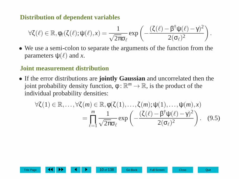
Distribution of dependent variables

∀ζ(ℓ) ∈ R,φℓ(ζ(ℓ);ψ(ℓ),x) =1√

2πσℓ

exp

(

−(ζ(ℓ)−β†ψ(ℓ)− γ)2

2(σℓ)2

)

.

• We use a semi-colon to separate the arguments of the functionfrom theparametersψ(ℓ) andx.

Joint measurement distribution

• If the error distributions arejointly Gaussian and uncorrelated then thejoint probability density function,φ : Rm→ R, is the product of theindividual probability densities:

∀ζ(1) ∈ R, . . . ,∀ζ(m) ∈ R,φ(ζ(1), . . . ,ζ(m);ψ(1), . . . ,ψ(m),x)

=m

∏ℓ=1

1√2πσℓ

exp

(

−(ζ(ℓ)−β†ψ(ℓ)− γ)2

2(σℓ)2

)

. (9.5)


9.1.2.6 Problem variables• After performing the trials, the values ofψ(ℓ) andζ(ℓ) are known and we

will re-interpret them as constants.• The unknowns are the parametersβ andγ in the relationship (9.1).• We have collected together these parameters into the vectorx and they

will be re-interpreted as the variables in our problem formulation sincethey are the values that are to be determined to solve our regressionproblem.


9.1.2.7 Maximum likelihood estimation• Need a criterion for choosing the “best value.”• Suppose that we are given:

– a collection of measurementsζ(1) ∈ R, . . . ,ζ(m) ∈ R,– values of the parametersx∈ Rn, and– a distanceδ ∈ R+.

• Suppose we take new measurements,ζ(1), . . . , ζ(m) using the samevalues of the independent variables

• Consider the probability that the new measurementsζ(1), . . . , ζ(m) lie inthe set:

S(x) = {ζ(1)∈R, . . . , ζ(m)∈R|ζ(ℓ)−δ≤ ζ(ℓ)≤ ζ(ℓ)+δ,∀ℓ= 1, . . . ,m}.• This probability is approximately equal to:

φ(ζ(1), . . . ,ζ(m);ψ(1), . . . ,ψ(m),x)(2δ)m.


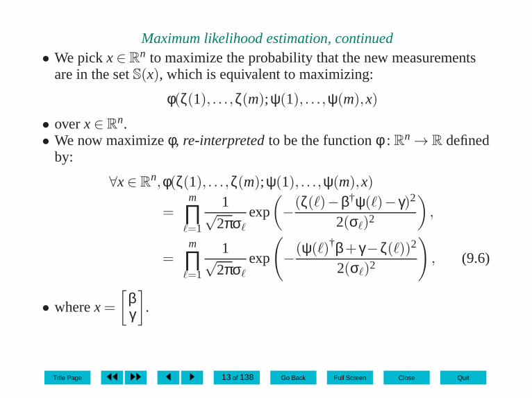
Maximum likelihood estimation, continued• We pickx∈ Rn to maximize the probability that the new measurements

are in the setS(x), which is equivalent to maximizing:

φ(ζ(1), . . . ,ζ(m);ψ(1), . . . ,ψ(m),x)

• overx∈ Rn.• We now maximizeφ, re-interpretedto be the functionφ : Rn → R defined

by:

∀x∈ Rn,φ(ζ(1), . . . ,ζ(m);ψ(1), . . .,ψ(m),x)

=m

∏ℓ=1

1√2πσℓ

exp

(

−(ζ(ℓ)−β†ψ(ℓ)− γ)2

2(σℓ)2

)

,

=m

∏ℓ=1

1√2πσℓ

exp

(

−(ψ(ℓ)†β+ γ−ζ(ℓ))2

2(σℓ)2

)

, (9.6)

• wherex=

[

βγ

]

.


9.1.2.8 Problem• The maximum likelihood estimation problem:

maxx∈Rn

φ(ζ(1), . . . ,ζ(m);ψ(1), . . .,ψ(m),x). (9.7)

9.1.3 Change of number of trials or correction of data• We may find that after solving the maximum likelihood estimation using

trials 1, . . . ,mwe conduct further trials or find that some of the data is inerror and needs to be corrected.

• We would like to be able obtain an updated estimation withoutstartingfrom scratch.


9.1.4 Problem characteristics9.1.4.1 Parameters re-interpreted as variables

• We have re-interpreted theparametersβ andγ of the probability densityin (9.5) to be thevariablesin our optimization problem.

• We interpretψ(ℓ) andζ(ℓ) to beknownvalues once the trials have beencompleted.

9.1.4.2 Objective• The objectiveφ(ζ(1), . . . ,ζ(m);ψ(1), . . . ,ψ(m),x) is the product of terms.• Each term in the product depends onx.

9.1.4.3 Number of parameters and trials• If m≤ n then there is no redundancy and we will not be able to reduce the

effects of measurement errors.

9.1.4.4 Generalizations• In some cases, we may have a non-linear relationship betweenthe

dependent and independent variables, as in (9.3).


9.2 Power system state estimation• We formulate anon-linear regressionproblem.

9.2.1 Motivation9.2.1.1 Non-linear regression

• Suppose that we hypothesize a non-linear relationship, such asζ = γ(ψ)β,between scalarsψ andζ with unknown parametersβ andγ.

• A standard approach for this particular non-linear relationship is to takelogarithms of both sides to form the equation:

ln(ζ) = β ln(ψ)+ ln(γ),Ψ = ln(ψ),Z = ln(ζ).


Non-linear regression, continued• We have implicitly defined an onto functionτ : R2

++ → R2 and atransformed functional relationship specified by:

∀[

ψζ

]

∈ R2++,τ

([

ψζ

])

=

[

ln(ψ)ln(ζ)

]

,

Z = βΨ+Γ.

• It is not always possible to find such a transformation.• For example, consider a functional relationship between scalarsψ andζ

of the form:

ζ = γ(ψ)β+δψ.

• We cannot transform this equation in a way such that all the unknownparametersβ,γ, andδ (or their transformed versions) appear linearly.

• Such a problem is called anon-linear regressionproblem.


9.2.1.2 Power system measurements• We may want to observe theactualstate of the system to check if the

system is operating within limits.• The state estimation problem involves finding the voltage angles and

magnitudes in the system that best match the measured values.


9.2.2 Formulation9.2.2.1 Measurements

• Real and reactive power injection at a bus;• Real and reactive power flow along a line; and• Voltage magnitude.

neutral

1 23

✚✙✛✘∼

P1,Q1,U1

P12,Q12

P13,Q13

t Y13t

t

load

Y23t

✚✙✛✘∼

Y12

Fig. 9.2. Three-buspower system stateestimation problem.


Real and reactive power injection

• LetB be the set of buses where there are measurements of the real andreactive power injections into the system.

• In Figure9.2, B= {1}.

Real and reactive line flow

• Let F be the set of lines where we have line flow measurements.• In Figure9.2, F= {(1,2),(1,3)}.

Voltage magnitude

• Finally, letU be the set of buses where there are voltage magnitudemeasurements.

• In Figure9.2, U= {1}.


9.2.2.2 Variables• Change the definition ofx in Section6.2 to include:

– the voltage angles at all buses except the reference bus, and– the voltage magnitudes at all buses in the system, includingthe

reference bus.• Now x∈ Rn, wheren is equal to one less than twice the number of buses,

so that the vectorx has been re-defined compared to Section6.2.


9.2.2.3 Measurement functions• Recall the definitions of the functionspℓ,qℓ : Rn → R in (6.12) and (6.13)

that were used in the power flow case study:

∀x∈ Rn, pℓ(x) = ∑

k∈J(ℓ)∪{ℓ}uℓuk[Gℓkcos(θℓ−θk)+Bℓksin(θℓ−θk)]−Pℓ,

∀x∈ Rn,qℓ(x) = ∑

k∈J(ℓ)∪{ℓ}uℓuk[Gℓksin(θℓ−θk)−Bℓkcos(θℓ−θk)]−Qℓ.

• Let us define new functions by omitting the values of the real and reactiveinjections,Pℓ andQℓ.

• That is, define ˜pℓ : Rn → R andqℓ : Rn → R to be:

∀x∈ Rn, pℓ(x) = ∑

k∈J(ℓ)∪{ℓ}uℓuk[Gℓkcos(θℓ−θk)+Bℓksin(θℓ−θk)],

∀x∈ Rn, qℓ(x) = ∑

k∈J(ℓ)∪{ℓ}uℓuk[Gℓksin(θℓ−θk)−Bℓkcos(θℓ−θk)].


9.2.2.4 Measurement functions• We denote the measurement functions by:

pℓ, qℓ, for the real and reactive power injection measurements, ℓ ∈ B,

pℓk, qℓk, for the real and reactive line flow measurements,(ℓ,k) ∈ F,

uℓ, for the voltage magnitude measurements, ℓ ∈ U.

• We collect the measurement functions into a vector functiong and collectthe measurements together into a corresponding vectorG:

∀x∈ Rn, g(x) =

[

pℓ(x)qℓ(x)

]

ℓ∈B[

pℓk(x)qℓk(x)

]

(ℓ,k)∈F[ uℓ(x) ]ℓ∈U

,G=

[

PℓQℓ

]

ℓ∈B[

PℓkQℓk

]

(ℓ,k)∈F[

Uℓ

]

ℓ∈U

.

• Let us define a new index setM that specifies all the measurements.• We re-index the entries of ˜g andG using the setM, so that ˜g= (gk)k∈M

andG∈ RM.


9.2.2.5 Error distribution• Assuming independent Gaussian measurement errors then we can write

the probability density,φ : RM → R, of the measurement vectorG as theproduct of probability densities:

∀G∈ RM,φ(G;x) = ∏

ℓ∈Bφpℓ(Pℓ;x)∏

ℓ∈Bφqℓ(Qℓ;x) ∏

(ℓ,k)∈Fφpℓk(Pℓk;x)

× ∏(ℓ,k)∈F

φqℓk(Qℓk;x)∏ℓ∈U

φuℓ(Uℓ;x),

• where each functionφpℓ(Pℓ;x),φqℓ(Qℓ;x),φpℓk(Pℓk;x),φqℓk(Qℓk;x), andφuℓ(Uℓ;x) represents the probability density function of the correspondingerror distribution and is parameterized byx.


Error distribution, continued• For example,

∀Pℓ ∈ R,φpℓ(Pℓ;x) =1√

2πσpℓ

exp

(

−(pℓ(x)− Pℓ)2

2(σpℓ)2

)

,

• whereσpℓ is the standard deviation of the measurement error of realpower at busℓ and where we have assumed that the expected error is zero.

• After the measurements are made, we can re-interpretφ to be a functionφ : Rn → R. That is, we re-interpretφ as being defined by:

∀x∈ Rn,φ(G;x) = ∏

ℓ∈Bφpℓ(Pℓ;x)∏

ℓ∈Bφqℓ(Qℓ;x) ∏

(ℓ,k)∈Fφpℓk(Pℓk;x)

× ∏(ℓ,k)∈F

φqℓk(Qℓk;x)∏ℓ∈U

φuℓ(Uℓ;x).

• Our maximum likelihood estimation problem is then:

maxx∈Rn

φ(G;x). (9.8)


9.2.3 Change in measurement data• We will consider how a change in measurement data affects theresult.

9.2.4 Problem characteristics9.2.4.1 Objective

• The objective of this problem is very similar to that of multi-variate linearregression Problem (9.7), except that each term in the product has one ofthe non-linear functions ˜pℓ, qℓ, pℓk, qℓk, or uℓ in the exponent instead of thelinear measurement equationψ(ℓ)†β+ γ.


9.2.4.2 Solvability• The measurements shown in the system illustrated in Figure9.2have just

enough information to determine all the values of the entries inx.• It is important to have redundancy of measurements in the system and to

“spread out” the measurements across the system as illustrated inFigure9.3.

neutral

1 23

✚✙✛✘∼

P1,Q1,U1

P12,Q12

P2,Q2,U2P3,Q3

t Y13t

t

load

Y23t

✚✙✛✘∼

Y12

Fig. 9.3. Three-buspower system stateestimation problemwith spread out mea-surements.


10Algorithms for unconstrained minimization

• In this chapter we will develop algorithms for unconstrained optimizationproblems of the form:

minx∈Rn

f (x),

• wherex∈ Rn and f : Rn → R.


Key issues• Descent directionsto reduce the value of the objective,• optimality conditions based ondescent directions,• optimality conditions forconvex objectives,• the development ofiterative algorithms, and• sensitivity analysis.


10.1 Optimality conditions10.1.1 Descent direction

10.1.1.1 Analysis

Definition 10.1 Let x∈ Rn and f : Rn → R. Then the vector∆x∈ Rn iscalled adescent directionfor f at x if:

∃α ∈ R++ such that(0< α ≤ α)⇒ ( f (x+α∆x)< f (x)).

✷


10.1.1.2 Example

∀x∈ R2, f (x) = (x1−1)2+(x2−3)2. (10.1)

−5 −4 −3 −2 −1 0 1 2 3 4 5−5

−4

−3

−2

−1

0

1

2

3

4

5

x1

x2

Fig. 10.1. Descentdirection (shown asthe longer arrow) fora function at a point

x =

[

21

]

, shown as

a ◦. The contours ofthe function decrease

towards x⋆ =

[

13

]

,

which is shown as a•.


10.1.1.3 Steepest descent step direction• ∆x=−∇f (x) is called the direction ofsteepest descent.

−5 −4 −3 −2 −1 0 1 2 3 4 5−5

−4

−3

−2

−1

0

1

2

3

4

5

x1

x2

Fig. 10.2. Steepestdescent directions fora function at variouspoints. The contours ofthe function decrease

towards x⋆ =

[

13

]

,

which is shown as a•.


10.1.1.4 Analysis

Lemma 10.1 Let f : Rn → R be partially differentiable with continuouspartial derivatives and letx∈ Rn, ∆x∈ Rn. Suppose that∇f (x)†∆x< 0.Then∆x is a descent direction for f atx.

Proof Let φ : R→ R be defined by:

∀t ∈ R,φ(t) = f (x+ t∆x).

By the chain rule,dφdt (t) =

∂ f∂x (x+ t∆x)∆x. Evaluating this att = 0 yields:

dφdt (0) =

∂ f∂x (x)∆x,

= ∇f (x)†∆x,= −2ε,

say, whereε > 0 by assumption.


Proof, continued But, by definition, sincef is partially differentiablewith continuous partial derivatives,

dφdt (0) = lim

α→0

f (x+α∆x)− f (x)α

.

Let α ∈ R++ be small enough such that

(0< |α| ≤ α)⇒(∣

∣

∣

∣


− dφdt (0)

∣

∣

∣

∣

≤ ε)

.

But this means that:

(0< |α| ≤ α)⇒(∣

∣

∣

∣


− (−2ε)∣

∣

∣

∣

≤ ε)

,

which implies that:

(0< |α| ≤ α)⇒(


≤−ε)

.


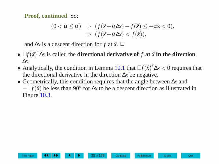
Proof, continued So:

(0< α ≤ α) ⇒ ( f (x+α∆x)− f (x)≤−αε < 0),⇒ ( f (x+α∆x) < f (x)),

and∆x is a descent direction forf at x. ✷

• ∇f (x)†∆x is called thedirectional derivative of f at x in the direction∆x.

• Analytically, the condition in Lemma10.1that∇f (x)†∆x< 0 requires thatthe directional derivative in the direction∆x be negative.

• Geometrically, this condition requires that the angle between∆x and−∇f (x) be less than 90◦ for ∆x to be a descent direction as illustrated inFigure10.3.


Descent directions

−5 −4 −3 −2 −1 0 1 2 3 4 5−5

−4

−3

−2

−1

0

1

2

3

4

5

x1

x2

Fig. 10.3. Variousdescent directions fora function a particu-

lar point x =

[

3−3

]

.

The contours decreasetowards the point

x⋆ =

[

13

]

, which is

shown as a•.


Corollary 10.2 Let x∈ Rn, let M∈ Rn×n be positive definite, and letf : Rn → R be partially differentiable with continuous partial derivativesand such that∇f (x) 6= 0. Then∆x=−M ∇f (x) is a descent direction forf at x.

Proof Note that∇f (x)†∆x=−∇f (x)†M ∇f (x)< 0, sinceM is positivedefinite and∇f (x) 6= 0. Apply Lemma10.1. ✷

• The “middle” arrow in Figure10.3shows the steepest descent stepdirection at ˆx, corresponding to the choiceM = I .

• The other directions correspond to other choices of positive definiteMand also yield descent directions in thatf is also reducing in thesedirections away from ˆx.


10.1.2 First-order conditions10.1.2.1 Necessary conditions

Theorem 10.3 Let f : Rn → R be partially differentiable with continuouspartial derivatives. If x⋆ is a local minimizer of f then∇f (x⋆) = 0.

Proof We prove the contra-positive. That is, we prove that if∇f (x⋆) 6= 0 thenx⋆ is not a local minimizer. LetM ∈ Rn×n be positivedefinite. By Corollary10.2, ∆x=−M ∇f (x⋆) is a descent direction forfatx⋆ and sox⋆ is not a local minimizer off . ✷

• The statement and proof of Theorem10.3, respectively, suggest twoapproaches to finding a minimizer off :

(i) solve∇f (x) = 0, or(ii) from the current pointx, move in the direction∆x=−M ∇f (x),

whereM is positive definite.


10.1.2.2 Example of insufficiency

−4 −3 −2 −1 0 1 2 3 4−10

−8

−6

−4

−2

0

2

4

6

8

10

xx ˆx x⋆

f (x)

Fig. 10.4. Graph of fand points (illustratedby the ◦) satisfying∇f (x) = 0 but whichmay or may not corre-spond to a minimum.


Example of insufficiency, continued

−4 −3 −2 −1 0 1 2 3 4−10

−8

−6

−4

−2

0

2

4

6

8

10

x

∇f (x)

x ˆx x⋆

Fig. 10.5. First deriva-tive ∇f of the functionfshown in Figure10.4.


Example of insufficiency, continued• ∇f (x) = 0 is not sufficient to guarantee a minimum.• We call points that satisfy∇f (x) = 0 critical points.• Not all critical points are minimizers.• For the function shown in Figure10.4:

(i) x=−3, f (x) = 8, a local maximizer and maximum off ,respectively,

(ii) ˆx= 0, f ( ˆx) = 0, ahorizontal inflection point of f , and(iii) x⋆ = 3, f (x⋆) =−8, a local minimizer and minimum off ,

respectively.


10.1.3 Second-order conditions10.1.3.1 Necessary conditions

Analysis

Theorem 10.4 Let f : Rn → R be twice partially differentiable withcontinuous second partial derivatives and suppose that x⋆ is a localminimizer of f . Then:

∇f (x⋆) = 0, (10.2)

∇2f (x⋆) is positive semi-definite. (10.3)

✷


Example

−4 −3 −2 −1 0 1 2 3 4−20

−15

−10

−5

0

5

10

15

20

x

∇2f (x)

x ˆx x⋆

Fig. 10.6. Secondderivative ∇2f of thefunction f shown inFigure10.4.


Example, continued

• Again consider the functionf shown in Figure10.4.• Its first and second derivatives are shown in Figures10.5and10.6,

respectively.• Since f : R→ R in this case, the Hessian∇2f : R→ R is positive

semi-definite if and only if it is non-negative.• The critical points off are at:

x=−3. At this point, the Hessian off , shown in Figure10.6, is negativeand hence not positive semi-definite. Therefore, by Theorem10.4, x=−3cannot be a local minimizer off .

ˆx= 0. At this point, the Hessian off is zero and hence positivesemi-definite. The second-order necessary conditions are satisfied but byinspection of Figure10.4, ˆx= 0 is clearly not a minimizer.

x⋆ = 3. This point is a local minimizer off . Figure10.6and Theorem10.4both concur that the Hessian is positive semi-definite.


10.1.3.2 Sufficient conditionsAnalysis

Theorem 10.5 Let f : Rn → R be twice partially differentiable withcontinuous second partial derivatives and suppose that:

∇f (x⋆) = 0,∇2f (x⋆) is positive definite.

Then x⋆ is a strict local minimizer of f .

Proof By hypothesis,∇2f (x⋆) is positive definite and∇2f is continuous.Therefore:

∃ε ∈ R++ such that(‖x⋆−x‖ ≤ ε)⇒ (∇2f (x) is positive definite).(10.4)

Let ∆x be any step direction such that 0< ‖∆x‖ ≤ ε and defineφ : R→ R

by:

∀t ∈ R,φ(t) = f (x⋆+ t∆x).


Proof, continued Then:

dφdt (t) =

∂ f∂x (x⋆+ t∆x)∆x,

dφdt (0) =

∂ f∂x (x⋆)∆x,

= ∇f (x⋆)†∆x,= 0, by hypothesis, (10.5)

d2φdt2

(t) = ∆x†∂2 f∂x2 (x⋆+ t∆x)∆x,

> 0,∀0< t ≤ 1, (10.6)

where the last inequality follows from (10.4) since∆x 6= 0 and since:

(0< t ≤ 1)⇒ (‖x⋆− (x⋆+ t∆x)‖= t ‖∆x‖ ≤ ‖∆x‖ ≤ ε).


Proof, continued We have thatφ(0) = f (x⋆) and:

∀∆x∈ Rn,(0< ‖∆x‖ ≤ ε)⇒

f (x⋆+∆x) = φ(1),

= φ(0)+∫ 1

t=0

dφdt (t)dt,

= φ(0)+∫ 1

t=0

[

dφdt (0)+

∫ t

t ′=0

d2φdt2

(t ′)dt′]

dt,

= φ(0)+ dφdt (0)+

∫ 1

t=0

∫ t

t ′=0

d2φdt2

(t ′)dt′dt,

= φ(0)+∫ 1

t=0

∫ t

t ′=0

d2φdt2

(t ′)dt′dt, by (10.5),

> f (x⋆), since the integrand is strictly positive by (10.6).

That is,x⋆ is a strict local minimizer.✷

• Positivesemi-definiteness of the second derivative matrix at a criticalpoint ˆx is not sufficient to guarantee thatˆx is a minimizer.


Example

• Continuing with the example from Section10.1.1.2, note that:

∀x∈ R2, f (x) = (x1−1)2+(x2−3)2,

∀x∈ R2,∇2f (x) =

[

2 00 2

]

,

• which is positive definite.

• Therefore, by Theorem10.5, the pointx⋆ =

[

13

]

is a strict local

minimizer of f .


Example of insufficiency

∀x∈ R, f (x) =−(x)4.

−1.5 −1 −0.5 0 0.5 1 1.5−5

−4

−3

−2

−1

0

1

x

f

ˆx

Fig. 10.7. A criticalpoint ˆx = 0, illustratedby the◦, where the sec-ond derivative matrix ispositive semi-definite atˆx yet the point is not aminimizer.


Example of insufficiency, continued

• Consider the pointx= 0 as illustrated in Figure10.7.• In this case:

∇f ( ˆx) = [−4( ˆx)3],

= [0],

∇2f ( ˆx) = [−12( ˆx)2],

= [0],

• so that:

∀∆x∈ R,0= ∆x∇2f ( ˆx)∆x≥ 0,

• and so∇2f ( ˆx) is positive semi-definite.• However,ˆx= [0] is clearly not a minimizer off .


10.1.4 Convex objectives10.1.4.1 First-order sufficient conditions

Analysis

• If f is twice partially differentiable with continuous partialderivativesand the second derivative matrix off is positive semi-definiteeverywherethen the objective is convex by Theorem2.7.


Corollary 10.6 Let f : Rn → R be convex and partially differentiable withcontinuous partial derivatives onRn and let x⋆ ∈ Rn. If ∇f (x⋆) = 0 thenf (x⋆) is the global minimum and x⋆ is a global minimizer of f .

Proof Recall Theorem2.6. The hypothesis of Theorem2.6 is satisfiedfor S= Rn. Consequently, (2.31) holds, which we repeat:

∀x,x′ ∈ S, f (x)≥ f (x′)+∇f (x′)†(x−x′).

Letting x′ = x⋆ andS= Rn in (2.31) and noting that∇f (x⋆) = 0, weobtain:

∀x∈ Rn, f (x)≥ f (x⋆).

That isx⋆ is a global minimizer off . ✷


Example

• Continuing with the example from Sections10.1.1.2and10.1.3.2, notethat∇2f is positive definite so thatf is convex.

• Therefore, by Corollary10.6, the pointx⋆ =

[

13

]

is the global minimizer

of f .


10.1.4.2 Uniqueness of minimizer

Theorem 10.7Let f : Rn → R be twice partially differentiable withcontinuous second partial derivatives onRn. If ∇2f is positive definitethroughoutRn andminx∈Rn f (x) possesses a minimum then theassociated minimizer is unique.

Proof Applying Theorems2.3and2.2to ∇f we find that there is atmost one point that satisfies the necessary conditions for minimizing f .Alternatively, Theorem2.7and Item(iii) of the conclusion ofTheorem2.4 imply the same result.✷


10.2 Approaches to finding minimizers10.2.1 Steepest descent

x(ν+1) = x(ν)−α(ν)∇f (x(ν)). (10.7)

10.2.1.1 Advantages

• Unless∇f (x(ν)) = 0, it is always possible to find a step-sizeα(ν) such thatthe objective will be reduced fromf (x(ν)) by updating the iterate tox(ν)−α(ν)∇f (x(ν)).

10.2.1.2 Example• Consider the quadratic function illustrated in Figure10.2.


Example, continued

∇f (x) =

[

2(x1−1)2(x2−3)

]

,

x(0) =

[

3−5

]

,

∇f (x(0)) =

[

2(3−1)2(−5−3)

]

,

=

[

4−16

]

,

x(1) = x(0)+α(0)∆x(0),

=

[

3−5

]

+α(0)[

−416

]

.

• If we setα(0) = 0.5 thenx(1) = x⋆ =

[

13

]

so that we would have reached

the minimizer in one iteration.


10.2.1.3 Disadvantages• Progress towards the solution may be very slow if the contoursets of the

function are very “eccentric.”

−5 −4 −3 −2 −1 0 1 2 3 4 5−5

−4

−3

−2

−1

0

1

2

3

4

5

x1

x2

Fig. 10.8. Scaled ver-sions of the steepestdescent step directionsfor an objective, definedin (10.8), with contoursets that are highlyeccentric ellipses. Thecontours of the func-tion decrease towards

x⋆ =

[

13

]

, which is

shown as a•.


10.2.1.4 Example• Figure10.8shows scaled versions of the steepest descent step directions

for a quadratic functionf : R2 → R defined by:

∀x∈ R2, f (x) = (x1−1)2+(x2−3)2−1.8(x1−1)(x2−3), (10.8)

=12

x†Qx+c†x+ constant,

Q = ∇2f (x),

=

[

2 −1.8−1.8 2

]

,

c =

[

3.4−4.2

]

.

• This function has the same minimizer,x⋆ =

[

13

]

, as the function in

Figure10.2, but has eccentric contour sets.• This function is more typical of functions encountered in practice.


Example, continued

• For a step-size ofα(ν), the next iterate has objective value:

f (x(ν+1)) = f (x(ν)−α(ν)∇f (x(ν))).

• Even if we chooseα(ν) at each iteration to minimizef(

x(ν)−α(ν)∇f (x(ν)))

exactlywith respect toα(ν), it can take manyiterations to find the minimum of a quadratic function havingeccentriccontour sets.

• The iterates will “zig-zag” back and forth across the axes ofthe eccentriccontour sets, making slow progress towardsx⋆.

• Non-quadratic functions with eccentric contour sets will exhibit similarlypoor behavior using the steepest descent step direction.


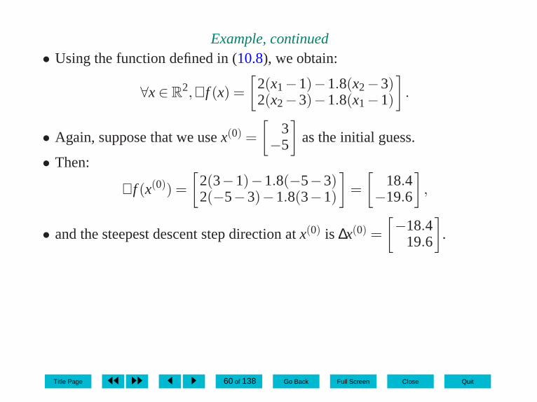
Example, continued• Using the function defined in (10.8), we obtain:

∀x∈ R2,∇f (x) =

[

2(x1−1)−1.8(x2−3)2(x2−3)−1.8(x1−1)

]

.

• Again, suppose that we usex(0) =

[

3−5

]

as the initial guess.

• Then:

∇f (x(0)) =

[

2(3−1)−1.8(−5−3)2(−5−3)−1.8(3−1)

]

=

[

18.4−19.6

]

,

• and the steepest descent step direction atx(0) is ∆x(0) =

[

−18.419.6

]

.


Example, continued• We update according to:

x(1) = x(0)+α(0)∆x(0) =

[

3−5

]

+α(0)[

−18.419.6

]

.

• For the value ofα(0) that minimizesf (x(0)+α(0)∆x(0)) over choices of

α(0), x(1) ≈[

−1.84670.1628

]

, which is relatively far from the minimizer off .

• Figure10.9illustrates the progress of iterations using steepest descent

step direction, starting atx(0) =

[

3−5

]

, and assuming that at theν-th

iteration the step-sizeα(ν) is chosen to minimizef (x(ν)+α(ν)∆x(ν)).• Figure10.9shows that after two iterations of steepest descent we are

close to the minimizer of this function.


Example, continued

−5 −4 −3 −2 −1 0 1 2 3 4 5−5

−4

−3

−2

−1

0

1

2

3

4

5

x1

x2

Fig. 10.9. Progressof iterations, shownas ◦, using steepestdescent step directionsfor an objective, definedin (10.8), with contoursets that are highlyeccentric ellipses. Thecontours of the func-tion decrease towards

x⋆ =

[

13

]

, which is

shown as a•. The initial

guess wasx(0) =

[

3−5

]

.


Example, continued

−5 −4 −3 −2 −1 0 1 2 3 4 5−5

−4

−3

−2

−1

0

1

2

3

4

5

x1

x2

Fig. 10.10. Progressof iterations, shownas ◦, using steepestdescent step directionsfor an objective, definedin (10.8), with contoursets that are highlyeccentric ellipses. Thecontours of the func-tion decrease towards

x⋆ =

[

13

]

, which is


guess wasx(0) =

[

−2−5

]

.


Example, continued

• However, starting atx(0) =

[

−2−5

]

, the progress is much slower, as

illustrated in Figure10.10, requiring six steepest descent step directionsto get close to the minimizer.

• In higher dimensions, withn larger than 2, the steepest descent algorithmwill repeatedly take us in directions that do not point directly towards theminimizer.

• The steepest descent step direction can be arbitrarily close to being atright anglesto the direction that points towards the minimizer.

• Moreover, we cannot expect to exactly minimizef (x(ν)+α(ν)∆x(ν)) overchoices ofα(ν) as assumed in Figures10.9and10.10.

• This typically increases further the number of iterations required to find auseful answer.


10.2.1.5 Example with non-quadratic objective

∀x∈ R2, f (x) = 0.01× (x1−1)4+0.01× (x2−3)4+(x1−1)2+(x2−3)2

−1.8(x1−1)(x2−3). (10.9)

−5 −4 −3 −2 −1 0 1 2 3 4 5−5

−4

−3

−2

−1

0

1

2

3

4

5

x1

x2

Fig. 10.11. Scaled ver-sions of the steepestdescent step directionsfor an objective, definedin (10.9), with contoursets that are perturbedeccentric ellipses. Thecontours of the functiondecrease towardsx⋆ =[

13

]

, which is shown as

a•.


Example with non-quadratic objective, continued

∀x∈ R2,∇f (x) =

[

0.04(x1−1)3+2(x1−1)−1.8(x2−3)0.04(x2−3)3−1.8(x1−1)+2(x2−3)

]

.


[

3−5

]


• Then,∇f (x(0)) =

[

18.72−40.08

]

and the steepest descent step direction atx(0)

is ∆x(0) =

[

−18.7240.08

]

.

• We update according to:

x(1) = x(0)+α(0)∆x(0) =

[

3−5

]

+α(0)[

−18.7240.08

]

.

• Figure10.12shows the progress of a steepest descent algorithm assumingthat at theν-th iteration the step-sizeα(ν) is chosen to minimizef (x(ν)+α(ν)∆x(ν)).



−5 −4 −3 −2 −1 0 1 2 3 4 5−5

−4

−3

−2

−1

0

1

2

3

4

5

x1

x2

Fig. 10.12. Progressof iterations, shownas ◦, using steepestdescent step directionsfor an objective, definedin (10.9), with contoursets that are perturbedeccentric ellipses. Thecontours of the func-tion decrease towards

x⋆ =

[

13

]

, which is


guess wasx(0) =

[

3−5

]

.


Example with non-quadratic objective, continued• Figure10.13shows the progress of a steepest descent algorithm starting

atx(0) =

[

−2−5

]

, again with the step-size chosen to minimize

f (x(ν)+α(ν)∆x(ν)) at each iteration.• The iterates again zig-zag back and forth across the axis of the contour

sets and many iterations are required to approach the minimizer.



−5 −4 −3 −2 −1 0 1 2 3 4 5−5

−4

−3

−2

−1

0

1

2

3

4

5

x1

x2

Fig. 10.13. Progressof iterations, shownas ◦, using steepestdescent step directionsfor an objective, definedin (10.9), with contoursets that are perturbedeccentric ellipses. Thecontours of the func-tion decrease towards

x⋆ =

[

13

]

, which is


guess wasx(0) =

[

−2−5

]

.


10.2.2 Solving∇f (x) = 0

• Another approach to minimizingf is based on the observation that∇f (x) = 0 is a system of either linear or non-linear equations having thesame number of equations as variables.

10.2.2.1 Linear first-order necessary conditions

Analysis

• Suppose thatf : Rn → R is quadratic of the form:

∀x∈ Rn, f (x) =

12

x†Qx+c†x,

• In this case, the equations∇f (x) = 0 are linear and of the formQx+c= 0.

• We can solve the equations:

Qx⋆ =−c.


Example

∀x∈ R2, f (x) = (x1−1)2+(x2−3)2−1.8(x1−1)(x2−3),

=12

x†Qx+c†x+ constant,

Q = ∇2f (x),

=

[

2 −1.8−1.8 2

]

,

c =

[

3.4−4.2

]

.

• SolvingQx⋆ =−c we obtain the minimizerx⋆ =

[

13

]

.


10.2.2.2 Non-linear first-order necessary conditionsAnalysis

• Apply the Newton–Raphson update to solve∇f (x) = 0.

∇2f (x(ν))∆x(ν) = −∇f (x(ν)),

x(ν+1) = x(ν)+α(ν)∆x(ν),

• The choice of step is called theNewton–Raphson step directiontominimize f .


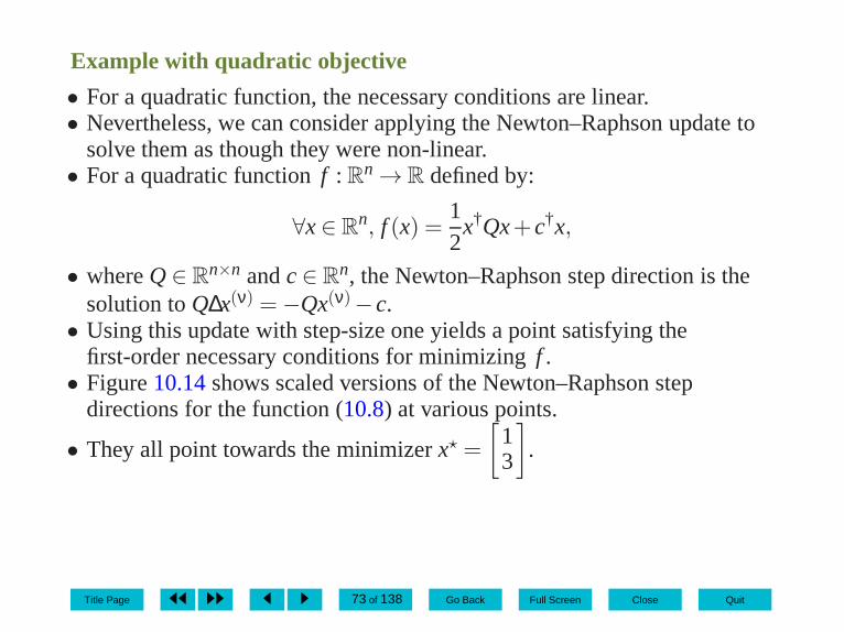
Example with quadratic objective

• For a quadratic function, the necessary conditions are linear.• Nevertheless, we can consider applying the Newton–Raphsonupdate to

solve them as though they were non-linear.• For a quadratic functionf : Rn → R defined by:

∀x∈ Rn, f (x) =

12

x†Qx+c†x,

• whereQ∈ Rn×n andc∈ Rn, the Newton–Raphson step direction is thesolution toQ∆x(ν) =−Qx(ν)−c.

• Using this update with step-size one yields a point satisfying thefirst-order necessary conditions for minimizingf .

• Figure10.14shows scaled versions of the Newton–Raphson stepdirections for the function (10.8) at various points.

• They all point towards the minimizerx⋆ =

[

13

]

.


Example with quadratic objective, continued

−5 −4 −3 −2 −1 0 1 2 3 4 5−5

−4

−3

−2

−1

0

1

2

3

4

5

x1

x2

Fig. 10.14. Scaled ver-sions of the Newton–Raphson step directionsfor an objective, definedin (10.8), with contoursets that are highly ec-centric ellipses. Thecontours of the functiondecrease towardsx⋆ =[

13

]

, which is shown as

a•.


Example with non-quadratic objective

∀x∈ R2, f (x) = 0.01(x1−1)4+0.01(x2−3)4+(x1−1)2+(x2−3)2

−1.8(x1−1)(x2−3),

∀x∈ R2,∇2f (x) =

[

0.12(x1−1)2+2 −1.8−1.8 0.12(x2−3)2+2

]

.


[

3−5

]


• The Newton–Raphson step direction atx(0) is the solution to:[

2.48 −1.8−1.8 9.68

]

∆x(0) =

[

−18.7240.08

]

,

∆x(0) ≈[

−5.2503.164

]

.



• We update according to:

x(1) = x(0)+α(0)∆x(0) =

[

3−5

]

+α(0)[

−5.2503.164

]

.

• For step-sizeα(0) = 1, we obtainx(1) =

[

−2.250−1.836

]

.

• Figure10.15shows the progress of a Newton–Raphson algorithm starting

atx(0) =

[

3−5

]

and assuming that at theν-th iteration the step-sizeα(ν)

were chosen to minimizef (x(ν)+α(ν)∆x(ν)).



−5 −4 −3 −2 −1 0 1 2 3 4 5−5

−4

−3

−2

−1

0

1

2

3

4

5

x1

x2

Fig. 10.15. Progress ofiterations, shown as◦,using Newton–Raphsonstep directions foran objective, definedin (10.9), with contoursets that are perturbedeccentric ellipses. Thecontours of the func-tion decrease towards

x⋆ =

[

13

]

, which is


guess wasx(0) =

[

3−5

]

.



• Figure10.16shows the progress of a Newton–Raphson algorithm starting

atx(0) =

[

−2−5

]

, again with the step-size chosen to minimize

f (x(ν)+α(ν)∆x(ν)) at each iteration.• The progress is much faster than for the steepest descent step direction for

the same value of initial guess.



−5 −4 −3 −2 −1 0 1 2 3 4 5−5

−4

−3

−2

−1

0

1

2

3

4

5

x1

x2

Fig. 10.16. Progress ofiterations, shown as◦,using Newton–Raphsonstep directions foran objective, definedin (10.9), with contoursets that are perturbedeccentric ellipses. Thecontours of the func-tion decrease towards

x⋆ =

[

13

]

, which is


guess wasx(0) =

[

−2−5

]

.


10.2.2.3 Advantages• Convergence to the solution of∇f (x) = 0 will be rapid, at least for initial

guesses that are near to a solution of the equations or after the iteratebecomes close to a solution of the equations.

• If f is quadratic then, as discussed in Section10.2.2.2, theNewton–Raphson step direction with step-sizeα(ν) = 1 takes us to acritical point in just one iteration.

• Since∇2f (x) is symmetric, we can take advantage of symmetry infactorization.


10.2.2.4 Disadvantages• For non-quadratic objectives and particularly at points that are far from

the minimizer, the Newton–Raphson step direction is not necessarily abetter direction than the steepest descent step direction.

• Factorization of the Hessian may require considerable effort if n is largeor the Hessian is dense.

• If ∇f (x(ν)) is not known analytically then it may be difficult or impossibleto directly calculate∇2f (x(ν)).

• If ∇2f (x(ν)) is not positive definite, then the Newton–Raphson updatemay take us towards a maximum or a point of inflection.


10.2.3 Generalization of Newton–Raphson and steepest descent• In this section we generalize the Newton–Raphson and steepest descent

updates in a way that can combine the advantages of each approach.

10.2.3.1 Uniform treatment of updates

∆x(ν) =−M ∇f (x(ν)), (10.10)

• with M ∈ Rn×n positive definite as in Corollary10.2to guarantee descent.• M = I yields the steepest descent step direction.

• M = [∇2f (x(ν))]−1

(if the Hessian∇2f is positive definite) yields theNewton–Raphson step direction.


10.2.3.2 Modified update

• To calculate∆x(ν) satisfying (10.10), we would solve the linear system:

∇2f (x(ν))∆x(ν) =−∇f (x(ν)). (10.11)

• Suppose that at thej-th stage of the factorization there are no positivediagonal pivots available.

• By Lemma5.4, this means that∇2f (x(ν)) is not positive definite, so thatthe Newton–Raphson step direction, even if it is defined, maynot be adescent direction.

• Let us modify the factorization by adding a positive quantity E j j to A( j)j j to

make the pivot positive, whereA( j) is the matrix obtained at thej-th stageof the factorization of∇2f (x(ν)).


Modified update, continued

• Adding E j j to A( j)j j is equivalent to adding the matrix:

E =

0...

0E j j

0...

0

(10.12)

• to ∇2f (x(ν)).• By construction,∇2f (x(ν))+E is symmetric and positive definite.

• Its inverseM = [∇2f (x(ν))+E]−1

exists and is also symmetric andpositive definite.

• By Corollary10.2, the search direction defined by (10.10) using thisM isa descent direction.

• This is called amodified factorization.


10.2.3.3 Further variations• We have considerable flexibility to either:

(i) construct positive definite approximations to[∇2f (x)]−1

, or(ii) approximately solve the equation:

∇2f (x)∆x=−∇f (x),

• in a way that guarantees that for the resulting∆x we have that∆x=−M∇f (x) for some positive definiteM.


10.2.4 Step-size10.2.4.1 Need for step-size selection

0 0.1 0.2 0.3 0.4 0.5 0.6 0.7 0.8 0.9 10

0.1

0.2

0.3

0.4

0.5

0.6

0.7

0.8

0.9

1

x

f

f (x(ν))

x(ν) xx(ν+1)

Fig. 10.17. The needfor a step-size rule. Thefunction f is illustratedwith a solid line to-gether with a quadraticapproximation to it,illustrated as a dashedline. The quadraticapproximation is asecond-order Taylorapproximation of faboutx(ν) = 0.3.


Need for step-size selection, continued• Suppose that we use the Newton–Raphson step direction to minimize the

function shown in Figure10.17, starting atx(ν) = 0.3.

∇2f (x(ν))∆x(ν) = −∇f (x(ν)),

∆x(ν) = 0.5.

• For this choice, ˇx= x(ν)+∆x(ν) = 0.8 minimizes the quadraticapproximation tof .

• However:

f (x) = f (x(ν)+∆x(ν))),

> f (x(ν)).

• A step-size ofα(ν) = 1 would lead to anincreasein the objective.


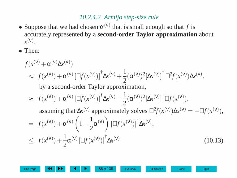
10.2.4.2 Armijo step-size rule

• Suppose that we had chosenα(ν) that is small enough so thatf isaccurately represented by asecond-order Taylor approximationaboutx(ν).

• Then:

f (x(ν)+α(ν)∆x(ν))

≈ f (x(ν))+α(ν) [∇f (x(ν))]†∆x(ν)+

12(α(ν))2[∆x(ν)]

†∇2f (x(ν))∆x(ν),

by a second-order Taylor approximation,

≈ f (x(ν))+α(ν) [∇f (x(ν))]†∆x(ν)− 1

2(α(ν))2[∆x(ν)]

†∇f (x(ν)),

assuming that∆x(ν) approximately solves∇2f (x(ν))∆x(ν) =−∇f (x(ν)),

= f (x(ν))+α(ν)(

1− 12

α(ν))

[∇f (x(ν))]†∆x(ν),

≤ f (x(ν))+12

α(ν) [∇f (x(ν))]†∆x(ν). (10.13)


Armijo step-size rule, continued• In practice, the reduction may not be as small as predicted by(10.13) and

we may have to accept a smaller reduction.• We choose an acceptance tolerance 0< δ < 1.• We start with tentative step-sizeα(ν) = 1 and calculate the trial objective

f (x(ν)+α(ν)∆x(ν)).• The step-size is accepted if:

f (x(ν)+α(ν)∆x(ν))≤ f (x(ν))+δ2

α(ν) [∇f (x(ν))]†∆x(ν). (10.14)

• Otherwise, reduce the step-size by a factor of, say, one halfand repeat theprocess until an iterate is produced that satisfies (10.14).


10.2.4.3 Wolfe condition• The rule for reducing the step-size discussed in the last section does not

check for “improvement” in the gradient∇f .• An alternative that makes use of gradient information rather than

objective values is provided by theWolfe condition:∣

∣

∣[∇f (x(ν)+α(ν)∆x(ν))]

†∆x(ν)

∣

∣

∣≤ η

∣

∣

∣[∇f (x(ν))]

†∆x(ν)

∣

∣

∣. (10.15)

• The Wolfe condition ensures that thedirectional derivative in thedirection∆x(ν) evaluated at the next iterate,[∇f (x(ν+1))]

†∆x(ν), is smallcompared to the directional derivative in the direction∆x(ν) at the current

iterate,[∇f (x(ν))]†∆x(ν).


10.2.4.4 Combined Armijo and Wolfe conditions

• The Wolfe condition (10.15) is often used in conjunction with the Armijocondition (10.14).

• The Armijo condition (10.14) ensures that the step-size is not so large asto invalidate the quadratic approximation of the objective.

• The Wolfe condition (10.15) ensures that the gradient of the objective isreduced sufficiently by the step.


10.2.4.5 Curve fitting• If f is relatively easy to evaluate, then we can evaluate it at several points

along the linex(ν)+α∆x(ν) for 0≤ α ≤ 1 and then fit a polynomial curve.

• We can minimize a quadratic function ofα using the following:

(i) If the coefficient of(α)2 in the quadratic function is positive, thenthe minimum of the function occurs at the pointx(ν)+α∆x(ν) for αsuch that the derivative of the quadratic function with respect toα isequal to zero. If this value ofα lies outside the range[0,1] then theclosest end-point should be selected.

(ii) If the coefficient of(α)2 in the quadratic function is negative, thenthe minimizer is one of the end-pointsα = 0 or α = 1.

10.2.4.6 Trust region• In a trust region approach the selection of an appropriate search

direction and step-size both explicitly consider the region over which asecond-order Taylor approximation represents the function f accurately.


10.2.5 Stopping criteria

• A typical criterion is to require that∥

∥

∥∇f (x(ν))

∥

∥

∥and

∥

∥

∥∆x(ν)

∥

∥

∥be

sufficiently small.• By Theorem2.6, if f is convex then any minimizerx⋆ of f (x) must

satisfy:

f (x⋆) ≥ f (x(ν))+ [∇f (x(ν))]†(x⋆−x(ν)),

≥ f (x(ν))−∣

∣

∣[∇f (x(ν))]

†(x⋆−x(ν))

∣

∣

∣,

≥ f (x(ν))−∥

∥

∥∇f (x(ν))∥

∥

∥

∥

∥

∥x⋆−x(ν)∥

∥

∥ . (10.16)

• If we know ana priori bound on the minimizer, then we can bound∥

∥

∥x⋆−x(ν)

∥

∥

∥independently ofx⋆ by someρ.

• We can ensure thatf (x(ν)) is within ε f of the value of the global

minimum by iterating until∥

∥

∥∇f (x(ν))

∥

∥

∥≤ ε f/ρ.


Stopping criteria, continued• The stopping criterion is often implemented in practice as aslightly

differentrelativecriterion by testing if:∥

∥

∥∇f (x(ν))∥

∥

∥≤ ε f

ρ

(

1+ | f (x(ν))|)

.


10.2.6 Avoiding critical points that are not minimizers• If, at some iterationν, we find that∇f (x(ν)) = 0 then our basic algorithm

cannot make further progress.• If f is convex, then by Corollary10.6, x(ν) is a minimizer andf (x(ν)) is a

minimum.• If f is not convex, then we may be at a point of inflection or a local

maximizer.


Avoiding critical points that are not minimizers, continued

• In Figure10.18, the iteratex(ν) = 0.5 is a horizontal inflection point of theobjective.

0 0.1 0.2 0.3 0.4 0.5 0.6 0.7 0.8 0.9 10.3

0.35

0.4

0.45

0.5

0.55

0.6

0.65

x

f

x(ν−1) x(ν)

Fig. 10.18. Iterate thatis a horizontal inflectionpoint of the objectivefunction.


Avoiding critical points that are not minimizers, continued• If the first-order necessary conditions are satisfied, but wecan detect that

the current iterate is not a minimizer, then we can restart the algorithm byperturbingx(ν) by a random amount to move it away from the point ofinflection or local maximum.

• Alternatively, at a horizontal inflection, we can use the previous iterate ina secant approximation as discussed in Section7.2.1.5, to seek a descentdirection.

• For example, in Figure10.18, using a secant approximation based onx(ν−1) andx(ν) would yield a descent direction.

• If we are not at a horizontal inflection point then another approach is tolook for negative eigenvalues of the Hessian and move in the direction ofthe corresponding eigenvector.


10.3 Sensitivity• Suppose that the objectivef is parameterizedby a parameterχ ∈ Rs.

That is, f : Rn×Rs→ R.• We imagine that we have solved the unconstrained minimization problem:

minx∈Rn

f (x;χ),

• for a base-case value of the parameters, sayχ = 0, to find the base-caseminimizerx⋆.

• We now consider the sensitivity of the minimizer and minimumtovariation of the parameters aroundχ = 0.


10.3.1 Implicit function theorem

Corollary 10.8 Let f : Rn×Rs→ R be twice partially differentiable withcontinuous second partial derivatives. Consider the minimizationproblem:

minx∈Rn

f (x;χ),

whereχ ∈ Rs is a parameter. Suppose that x⋆ is a local minimizer of thisproblem for the base-case value of the parametersχ = 0. We call x= x⋆

a base-case minimizer. Define the (parameterized) Hessian∇2

xxf : Rn×Rs→ Rn×n by:

∀x∈ Rn,∀χ ∈ R

s,∇2xxf (x;χ) = ∂2 f

∂x2 (x;χ).

Suppose that∇2xxf (x

⋆;0) is positive definite, so that x⋆ satisfies thesecond-order sufficient conditions for the base-case problem. Then, thereis a local minimizer of f(x;χ) for χ in a neighborhood of the base-casevalues of the parametersχ = 0 and the local minimizer is a partiallydifferentiable function ofχ in this neighborhood. The sensitivity of the


local minimizer x⋆ with respect to variation of the parametersχ,evaluated at the base-caseχ = 0, is given by:

∂x⋆

∂χ (0) =−[∇2xxf (x

⋆;0)]−1

K(x⋆;0),

where K: Rn×Rs→ Rn×s is defined by:

∀x∈ Rn,∀χ ∈ R

s,K(x;χ) = ∂2 f∂x∂χ(x;χ).

The sensitivity of the corresponding local minimum f⋆ to variation of theparametersχ, evaluated at the base-caseχ = 0, is given by:

∂ f ⋆

∂χ (0) =∂ f∂χ (x⋆;0).

If f (•;χ) is convex for eachχ in a neighborhood of0 then the minimizersand minima are global in this neighborhood.


Proof The sensitivity of the local minimizer follows fromCorollary7.5, noting that by assumption the Hessian is positive definitein a neighborhood of the base-case minimizer and parameters.The sensitivity of the local minimum follows by totally differentiatingthe value of the local minimumf ⋆(χ) = f (x⋆(χ);χ) with respect toχ. Inparticular,

∂ f ⋆

∂χ (0) =d f(x⋆(χ);χ)dχ (0),

=∂ f∂χ (x⋆;0)+

∂ f∂x (x⋆;0)

∂x⋆

∂χ (0),

on totally differentiatingf (x⋆(χ);χ) with respect toχ,

=∂ f∂χ (x⋆;0),

since the first-order necessary conditions at the base-caseare∂ f∂x (x⋆;0) = 0.

The global results follow from Corollary10.6. ✷


Discussion

• If ∇2xxf (x

⋆;0) has already been factorized then each sensitivity ofx⋆ withrespect to an entry ofχ requires only a forwards and backwardssubstitution.

• The sensitivity of the local minimum is calledthe envelope theorem.


10.3.2 Example• Consider the parameterized objective functionf : R2×R→R defined by:

∀x∈R2,∀χ ∈ R, f (x;χ) = (x1−exp(χ))2+(x2−3exp(χ))2+5χ.

• This is a parameterized version of the function defined in (10.1).• For χ = 0, the parameterized function is the same as the function defined

in (10.1) and from the discussion in Section10.1.1.2we know that the

base-case unconstrained minimizer isx⋆ =

[

13

]

.

• By Corollary10.8, there is a minimizer off (•;χ) for χ in a neighborhoodof the base-case value of the parameterχ = 0 and the minimizer is adifferentiable function ofχ in this neighborhood.

• The sensitivity of the minimizerx⋆ with respect to variation of theparameterχ, evaluated at the base-caseχ = 0, is given by:

∂x⋆

∂χ (0) =−[∇2xxf (x

⋆;0)]−1

K(x⋆;0),


Example, continued• where∇2

xxf : R2×R→ R2×2 andK : R2×R→ R2×1 are defined by:

∀x∈ R2,∀χ ∈ R,∇2

xxf (x;χ) =∂2 f∂x2 (x;χ),

=

[

2 00 2

]

,

∇2xxf (x

⋆;0) =

[

2 00 2

]

,

∀x∈ R2,∀χ ∈ R,K(x;χ) =

∂2 f∂x∂χ(x;χ),

=

[

−2exp(χ)−6exp(χ)

]

,

K(x⋆;0) =

[

−2−6

]

,

• where we observe that∇2xxf (x

⋆;0) is positive definite.


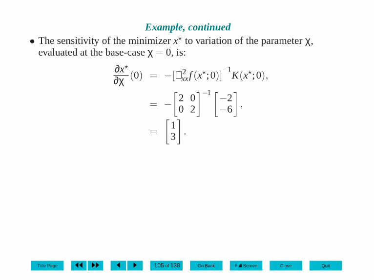
Example, continued• The sensitivity of the minimizerx⋆ to variation of the parameterχ,

evaluated at the base-caseχ = 0, is:

∂x⋆

∂χ (0) = −[∇2xxf (x

⋆;0)]−1

K(x⋆;0),

= −[

2 00 2

]−1[−2−6

]

,

=

[

13

]

.


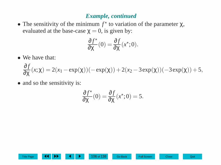
Example, continued• The sensitivity of the minimumf ⋆ to variation of the parameterχ,

evaluated at the base-caseχ = 0, is given by:

∂ f ⋆

∂χ (0) =∂ f∂χ (x⋆;0).

• We have that:

∂ f∂χ (x;χ) = 2(x1−exp(χ))(−exp(χ))+2(x2−3exp(χ))(−3exp(χ))+5,

• and so the sensitivity is:

∂ f ⋆

∂χ (0) =∂ f∂χ (x⋆;0) = 5.


10.4 Summary

• Descent directions,• Optimality conditions,• Algorithms,• Sensitivity analysis.


11Solution of the unconstrained minimization case

studies

• Multi-variate linear regression case study in Section11.1, and• Power system state estimation case study in Section11.2.


11.1 Multi-variate linear regression11.1.1 Transformation of objective

• Recall Problem (9.7):

maxx∈Rn

φ(ζ(1), . . . ,ζ(m);ψ(1), . . . ,ψ(m),x),

• whereφ : Rn → R was defined in (9.6), which we repeat here:

∀x∈ Rn,φ(ζ(1), . . . ,ζ(m);ψ(1), . . .,ψ(m),x)

=m

∏ℓ=1

1√2πσℓ

exp

(

−(ψ(ℓ)†β+ γ−ζ(ℓ))2

2(σℓ)2

)

.

• First definef : Rn → R by:

∀x∈ Rn, f (x) =− ln(φ(ζ(1), . . . ,ζ(m);ψ(1), . . .,ψ(m),x)).


Transformation of objective, continued

• Then:

∀x∈ Rn, f (x) = − ln

(

m

∏ℓ=1

1√2πσℓ

exp

(

−(ψ(ℓ)†β+ γ−ζ(ℓ))2

2(σℓ)2

))

,

= −m

∑ℓ=1

[

ln

(

1√2πσℓ

)

− (ψ(ℓ)†β+ γ−ζ(ℓ))2

2(σℓ)2

]

,

=m

∑ℓ=1

[

(ψ(ℓ)†β+ γ−ζ(ℓ))2

2(σℓ)2

]

−m

∑ℓ=1

ln

(

1√2πσℓ

)

,

• where we recall that:

x=

[

βγ

]

∈ Rn.


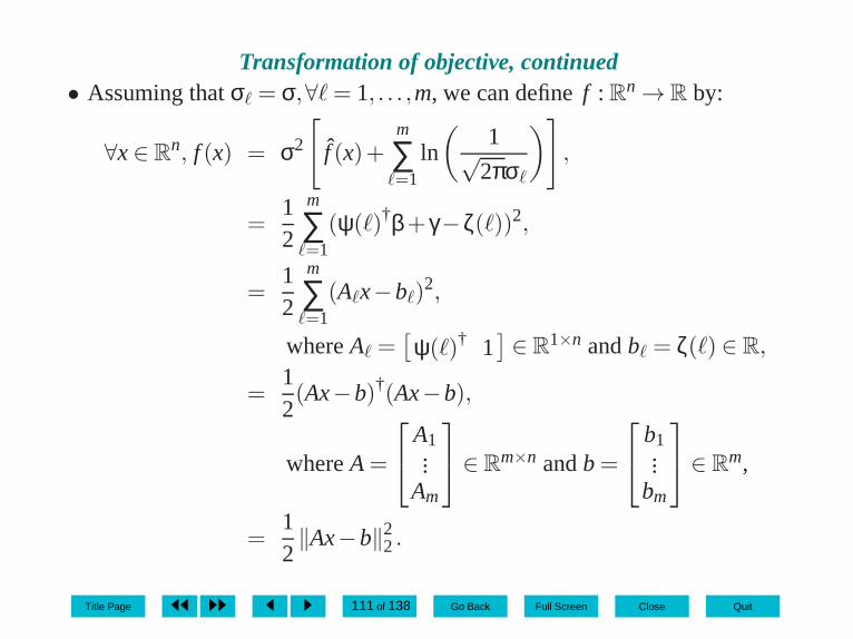
Transformation of objective, continued• Assuming thatσℓ = σ,∀ℓ= 1, . . . ,m, we can definef : Rn → R by:

∀x∈ Rn, f (x) = σ2

[

f (x)+m

∑ℓ=1

ln

(

1√2πσℓ

)

]

,

=12

m

∑ℓ=1

(ψ(ℓ)†β+ γ−ζ(ℓ))2,

=12

m

∑ℓ=1

(Aℓx−bℓ)2,

whereAℓ =[

ψ(ℓ)† 1]

∈ R1×n andbℓ = ζ(ℓ) ∈ R,

=12(Ax−b)†(Ax−b),

whereA=

A1...

Am

∈ Rm×n andb=

b1...

bm

∈ Rm,

=12‖Ax−b‖2

2 .


Transformation of objective, continued• By Theorem3.1, so long as either:

(i) Problem (9.7) has a maximum or(ii) the problem:

minx∈Rn

f (x), (11.1)

has a minimum,• then they both have the same set of optimizers.• Problem (11.1) involves minimizing (half of) the sum of squares of linear

functions ofx and is called alinear least-squares problem.• We refer to the corresponding specification of the affine function defined

in (9.1) as aleast-squares fitto the data.• The necessary conditions for a minimum of Problem (11.1) are a set of

linear simultaneous equations.


11.1.2 Comparison of objectives• The necessary conditions for a minimum of Problem (11.1) are a set of

linear simultaneous equations.• In contrast, the necessary conditions for a maximum of Problem (9.7) are

a set of non-linear simultaneous equations sinceφ is non-quadratic.

11.1.3 Derivatives of objective

∀x∈ Rn,∇f (x) = A†(Ax−b), (11.2)

∀x∈ Rn,∇2f (x) = A†A. (11.3)


11.1.4 Optimality conditions• ∇2f (x) is positive semi-definite.• Therefore the objectivef is convex.• First-order conditions are sufficient.• Solving either Problem (11.1) or Problem (9.7) yields the same set of

minimizers.

• In summary, by solving∇f (x) = 0 for x⋆ =

[

β⋆

γ⋆]

we will find a

maximizer of Problem (9.7).• Setting∇f (x) = 0 and re-arranging, we obtain:

Ax= B , (11.4)

• whereA = A†A andB = A†b.


11.1.5 Further transformation• The condition number ofA†A can be large.• Instead of calculating and factorizingA†A, weQRfactorizeA itself to

obtain (ignoring any permutations of the rows or columns ofA):

A= QR,

• with Q∈ Rm×m unitary,R=

[

U0

]

∈ Rm×n upper triangular, with

U ∈ Rn×n upper triangular andU is non-singular ifA has linearlyindependent columns.

• We have:

∀x∈ Rn, f (x) =

12(Ax−b)†(Ax−b),

=12(x†A†−b†)(Ax−b),

=12(x†R†Q†−b†)(QRx−b), by definition ofQR,


Further transformation, continued

=12(x†R†Q†−b†QQ†)(QRx−QQ†b), sinceQ is unitary,

=12(x†R†−b†Q)Q†Q(Rx−Q†b), on factorizing,

=12(x†R†−b†Q)(Rx−Q†b), becauseQ is unitary,

=12

(

x†[

U0

]†

−b†Q

)

([

U0

]

x−Q†b

)

, whereR=

[

U0

]

,

=12

∥

∥

∥

∥

[

U0

]

x−Q†b

∥

∥

∥

∥

2

2,

=12

∥

∥

∥

∥

∥

[

U0

]

x−[

[Q‖]†

[Q⊥]†

]

b

∥

∥

∥

∥

∥

2

2

, whereQ=[

Q‖ Q⊥ ],

with Q‖ ∈ Rm×n′,Q⊥ ∈ Rm×(m−n′),



=12

∥

∥

∥

∥

∥

[

Ux− [Q‖]†b

0x− [Q⊥]†b

]∥

∥

∥

∥

∥

2

2

,

=12

∥

∥

∥Ux− [Q‖]

†b∥

∥

∥

2

2+

12

∥

∥

∥[Q⊥]

†b∥

∥

∥

2

2, by definition of theL2 norm.

• Geometrically, we have resolved the vectorAx−b into the sum of twovectors:

Ux− [Q‖]†b, which depends onx, and

0x− [Q⊥]†b=−[Q⊥]

†b, which does not depend onx.

• The columnsQ‖ are such that[Q‖]†b “aligns” with Ux.

• The columnsQ⊥ are such that(−[Q⊥]†b) is perpendicular toUx.

• If U is non-singular then the first-order necessary conditions for

minimizing∥

∥

∥Ux− [Q‖]

†b∥

∥

∥

2

2areUx= [Q‖]

†b.



✻

Ux′− [Q‖]†b

✻

Ux′′− [Q‖]†b

✲

−[Q⊥]†b

✟✟✟✟✟✟✟✟✟✟✟✟✟✟✟✟✟✟✟✟✟✟✟✟✯

Ax′−b

✘✘✘✘✘✘✘✘✘✘✘✘✘✘✘✘✘✘✘✘✘✘✘✘✿

Ax′′−b

Fig. 11.1. Resolutionof the vector Ax − binto two perpendicularvectors for the valuesx= x′ andx= x′′.


Further transformation, continued• We can obtain the solution to Problem (11.1) by:

– evaluatingy⋆ = [Q‖]†b, and

– performing a backwards substitution to solveUx⋆ = y⋆.

• The solutionx⋆ =

[

β⋆

γ⋆]

specifies the maximum likelihood estimate of the

relationship between the independent and dependent variables:

∀ψ ∈ Rn−1,ζ = [β⋆]†ψ+ γ⋆.


11.1.6 Relationship of optimality conditions to linear regression• In designing the values ofψ(ℓ) for the trials, there are two related issues

to be addressed:

(i) Providing enough variety in the trials to ensure that∇2f = A†A ispositive definite. We discuss this issue in Sections11.1.6.1and11.1.6.2.

(ii) Providing enough redundancy so that the effects of measurementerror can be “averaged out.” We discuss this briefly inSection11.1.6.3.


11.1.6.1 Insufficient variety in the trials• If ∇2f (x) is singular then there will be many possible values of the

parametersx that satisfy the maximum likelihood criterion in themodel (9.1), based on the data from trialsℓ= 1, . . . ,m.

11.1.6.2 Sufficient variety in the trials• On the other hand, if there is ann element subset{ℓ1, ℓ2, . . . , ℓn} of the

trials{1, . . . ,m} such that then rows ofA corresponding to these trials arelinearly independent, then∇2f (x) = A†A is non-singular.

11.1.6.3 Redundancy and validation of model• We may want to find not only the maximum likelihood estimator but also

estimate the variance of the error.• In general, it requires thatm be larger, and typically considerably larger,

thann.


11.1.7 Changes in the problem11.1.7.1 Additional trials

• If additional trials are added then there will be additionalrows added toAand additional entries added tob, necessitating factorization of theaugmentedA.


11.1.7.2 Sensitivity• We consider the sensitivity of the coefficientsβ⋆ andγ⋆ to changes in the

measurements.• That is, for eachℓ= 1, . . . ,m, we will imagine that theℓ-th measurement

is actuallyζ(ℓ)+χℓ, with χ ∈ Rm.• We calculate the sensitivity ofβ⋆ andγ⋆ to χ, evaluated atχ = 0.• By Corollary10.8, the sensitivity of the minimizerx⋆ is given by:

∂x⋆

∂χ (0) =−[∇2xxf (x

⋆;0)]−1

K(x⋆;0),

• where∇2xxf : Rn×Rm→ Rn×n andK : Rn×Rm→ Rn×m are defined by:

∀x∈ Rn,∀χ ∈ R

m,∇2xxf (x;χ) =

∂2 f∂x2 (x;χ),

= A†A,

∀x∈ Rn,∀χ ∈ R

m,K(x;χ) =∂2 f∂x∂χ(x;χ),

= −A†.


Sensitivity, continued

• That is, the sensitivity toχℓ is given by[A†A]−1

A†I ℓ, whereI ℓ ∈ Rm is avector with zeros in all places except theℓ-th place, which is a one.

• This is the same as the solution of a regression problem that had the samevalues of independent variables as in the base-case, but where the vectorof measurements was changed fromb to I ℓ.

• Using the analysis in Section11.1.5, we can calculate the sensitivity toχℓ

by:

– evaluatingy= [Q‖]†I ℓ, and

– performing a backwards substitution to solveU∂x⋆

∂χ (0) = y.


11.2 Power system state estimation11.2.1 Transformation of objective

• We use a similar transformation to the one in Section11.1.• We define:

∀x∈ Rn, f (x) = − lnφ(G;x)+ ∑

ℓ∈Mln

1√2πσℓ

, (11.5)

∀x∈ Rn, f (x) = ∑

ℓ∈M

(gℓ(x)− Gℓ)2

2σ2ℓ

,

=12(g(x)− G)

†[Σ]−2(g(x)− G), (11.6)

• where:Σ ∈ RM×M is the diagonal matrix withℓ-th diagonal entry equal to

σℓ, ℓ ∈M,g : Rn → RM is the vector of all measurement functions, andG∈ RM is the vector of all measurements.


Transformation of objective, continued• The transformed problem is:

minx∈Rn

f (x). (11.7)

• We have a least-squares problem since the objective is the sum of squaresof terms.

• Since each term(g(x)− G) is non-linear, we classify Problem (11.7) as anon-linear least-squares problem.


11.2.2 Derivatives of objective

∀x∈ Rn,∇f (x) = J(x)†

[Σ]−2(g(x)− G),

= ∑ℓ∈M

∇gℓ(x)[Σℓ]−2(gℓ(x)− Gℓ), (11.8)

∀x∈ Rn,∇2f (x) = J(x)†

[Σ]−2J(x)+ ∑ℓ∈M

∇2gℓ(x)[Σℓ]−2(gℓ(x)− Gℓ),

(11.9)

• whereJ is the Jacobian of ˜g and∇gℓ is the transpose of theℓ-th row of J.


11.2.3 Optimality conditions and algorithms11.2.3.1 Qualitative comparison between Problems (9.8) and (11.7)

• The first-order necessary conditions for Problem (9.8), ∇φ(G;x) = 0, arenon-linear.

• The first-order necessary conditions for Problem (11.7), ∇f (x) = 0, arealso non-linear.

• Consider the measurement functions in detail:(i) Each voltage magnitude measurement function, ˜uk(x) = uk, is

linear.(ii) The real and reactive injection measurement functionsand the real

and reactive flow measurement functions areapproximatelylinear.This observation and the expression for∇f , (11.8), mean that thenecessary conditions for Problem (11.7), ∇f (x) = 0, are alsoapproximately linear.

• The transformation (11.5) transforms a non-linear objective into anapproximatelyquadratic objective.


Qualitative comparison between Problems (9.8) and (11.7), continued• The necessary conditions for minimizing Problem (11.7) are

approximatelylinear.• We use the hypotheses of the chord and Kantorovich theorems to

qualitativelycompare the convergence properties of the Newton–Raphsonupdate applied to:– Problem (9.8); that is,∇φ(x) = 0, and– Problem (11.7); that is,∇f (x) = 0.

• Since∇f is approximately linear, then∇2f is approximately constant anda Lipschitz constant can be found for∇2f that is smaller than a Lipschitzconstant for∇2φ.

• We expect the radiiρ−,ρ+, andρ defined in Theorems7.3and7.4 to belarger for the problem of solving∇f (x) = 0 than for the problem ofsolving∇φ(x) = 0.

• That is, we can expect to converge to a solution from a poorer initialguess if we apply the chord or Newton–Raphson methods to solve∇f (x) = 0 instead of applying it to solve∇φ(x) = 0.


11.2.3.2 Problem (11.7)Hessian

• The Hessian∇2f from (11.9) consists of the sum of two terms:

(i) J(x)†[Σ]−2J(x), which is of the formA†A for A= [Σ]−1J(x) and so

the matrixJ(x)†[Σ]−2J(x), is positive semi-definite, and(ii) ∑ℓ∈M∇2gℓ(x)[Σℓ]

−2(gℓ(x)− Gℓ), which can turn out to be notpositive semi-definite.

Search direction

• Recall that in defining a search direction, we found that∆x(ν) =−M∇f (x(ν)) is a descent direction ifM is positive definite.

• We know thatJ(x)†[Σ]−2J(x) is positive semi-definite, but we do not

know if the Hessian is positive semi-definite.• Instead of using the exact Newton–Raphson update, we approximate∇2f

by its first term:

J(x)†[Σ]−2J(x). (11.10)


Search direction, continued

• We solve for the approximate update direction:

J(x(ν))†[Σ]−2J(x(ν))∆x(ν) = −∇f (x(ν)),

= J(x(ν))†[Σ]−2(G− g(x(ν))). (11.11)

• This approximation is called theGauss–Newton method.• We must still consider the possibility thatJ(x(ν))

†[Σ]−2J(x(ν)) is not

positive definite.• We can follow the approach discussed in Section10.2.3.2and add terms

to the diagonal of the matrix during factorization to ensurethat themodified matrix is positive definite.


Search direction by solving a related linear least-squaresproblem

• The use of (11.11) to calculate a search direction suffers from a similardrawback to the solution of (11.4) in the linear case.

• By definingA= [Σ]−1J(x(ν)) andb= [Σ]−1(G− g(x(ν))), note that (11.11)is equivalent toA†A∆x(ν) = A†b, which is the same form as the optimalitycondition for the multi-variate linear regression problem.

• We can therefore find∆x(ν) by noting that∆x(ν) is the solution to thelinear least-squares problem:

min∆x∈Rn

12‖A∆x−b‖2

2 . (11.12)


Levenberg–Marquardt

• An alternative approach is to approximate the possibly not positivesemi-definite term∑ℓ∈M∇2gℓ(x)[Σℓ]

−2(gℓ(x)− Gℓ) by the positivedefinite matrixλI , whereλ > 0 is chosen to be large enough to make theresulting approximation of the Hessian positive definite.

• This is called theLevenberg–Marquardt method. and is related to thetrust region approach mentioned in Section10.2.4.

Further approximation

• We can further approximateJ using the using the fast-decoupled or otherapproximations to the Jacobian of the power flow equations, as in thediscussion of the solution of the power flow equations in Section 8.2.4.2.


11.2.4 Placement of meters in the system11.2.4.1 Insufficient variety in the measurements

neutral

1 23

✚✙✛✘∼

P1,Q1,U1

P12,Q12

P13,Q13

t Y13t

t

load

Y23t

✚✙✛✘∼

Y12

Fig. 11.2. The three-bus power systemstate estimation prob-lem, repeated fromFigure9.2.


Insufficient variety in the measurements, continued• If the measurements are not spread out throughout the systemor if there

is a measurement failure, thenJ(x)†[Σ]−2J(x) can be singular.

• For example, consider the system in Figure9.2, which is repeated inFigure11.2.

• The are five unknown variables:u1,θ2,u2,θ3, andu3.• There are seven measurements:P1,Q1,U1, P12,Q12, P13, andQ13.• However, since:

p1(x) = p12(x)+ p13(x),q1(x) = q12(x)+ q13(x),

• there is redundant information concerning bus 1.• This would enable us to estimate the voltage magnitude and flows around

node 1, even in the presence of measurement errors.• There is just enough information to estimate all the voltageand flows in

the system.


Insufficient variety in the measurements, continued• Suppose that there is a failure of the voltage measurement inthe system

in Figure11.2.• In this case, there will be many sets of voltages and anglesθ2, |v2|,θ3, and|v3| that are consistent with maximizing the likelihood of the observedmeasurements.

• We say that the system isunobservable.• If we aredesigninga measurement system, then singularity of

J(x)†[Σ]−2J(x) for a candidate meter placement plan suggests that weshould add more meters to the plan.

• If we areoperatinga measurement system and we find that because of,for example, meter failures, the matrixJ(x)†

[Σ]−2J(x) is singular, then wecannot estimate the state completely.

• In practice, in the latter case, the user of the software usually specifiespseudo-measurements; that is, guesses at what the actual measurementwould be, based on experience, so that a rough estimate of thecompletestate can be found.


11.2.4.2 Sufficient variety in the measurements

neutral

1 23

✚✙✛✘∼

P1,Q1,U1

P12,Q12

P2,Q2,U2P3,Q3

t Y13t

t

load

Y23t

✚✙✛✘∼

Y12

Fig. 11.3. The three-bus power system stateestimation problemwith spread out mea-surements repeatedfrom Figure9.3.


Sufficient variety in the measurements, continued• Usually, if there is sufficient variety in the measurements,the positive

semi-definite matrixJ(x)†[Σ]−2J(x) will turn out to be positive definite for

almost all, if not all values ofx, and hence be non-singular.• If it is non-singular then the approximate update equation (11.11) has a

unique solution.• For example, for the arrangement in Figure9.3, which is repeated in

Figure11.3, for almost all values ofx there is a five element subset of therows of J(x) that is linearly independent, so thatJ(x)†

[Σ]−2J(x) isnon-singular.

• This remains true even in the presence of a single failure of avoltagemeasurement.

11.2.4.3 Sensitivity• We can consider variation of the estimate with variation in the

measurement data.


applied optimization: formulation and algorithms for...

Documents