Applied Mathematical Sciences Volume 49

Editors F. John J. E. Marsden 1. Sirovich

Advisors H. Cabannes M. Ghil J. K. Hale J. Keller J. P. LaSalle G. B. Whitham

Applied Mathematical Sciences A Selection

21. Courant/Friedrichs: Supersonic Flow and Shock Waves. 22. Rouche/Habets/Laloy: Stability Theory by Liapunov's Direct Method. 23. Lamperti: Stochastic Processes: A Survey of the Mathematical Theory. 24. Grenander: Pattern Analysis: Lectures in Pattern Theory, Vol. II. 25. Davies: Integral Transforms and Their Applications, 2nd ed. 26. Kushner/Clark: Stochastic Approximation Methods for Constrained and

Unconstrained Systems. 27. de Boor: A Practical Guide to Splines. 28. Keilson: Markov Chain Models-Rarity and Exponentiality. 29. de Veubeke: A Course in Elasticity. 30. Sniatycki: Geometric Quantization and Quantum Mechanics. 31. Reid: Sturmian Theory for Ordinary Differential Equations. 32. Meis/Markowitz: Numerical Solution of Partial Differential Equations. 33. Grenander: Regular Structures: Lectures in Pattern Theory, Vol. III. 34. Kevorkian/Cole: Perturbation Methods in Applied Mathematics. 35. Carr: Applications of Centre Manifold Theory. 36. Bengtsson/Ghil/Kallen: Dynamic Meterology: Data Assimilation Methods. 37. Saperstone: Semidynamical Systems in Infinite Dimensional Spaces. 38. Lichtenberg/Lieberman: Regular and Stochastic Motion. 39. Piccinini/StampacchialVidossich: Ordinary Differential Equations in R". 40. Naylor/Sell: Linear Operator Theory in Engineering and Science. 41. Sparrow: The Lorenz Equations: Bifurcations, Chaos, and Strange Attractors. 42. Guckenheimer/Holmes: Nonlinear OSCillations, Dynamical Systems and

Bifurcations of Vector Fields. 43. OckendoniTayler: Inviscid Fluid Flows. 44. Pazy: Semigroups of Linear Operators and Applications to Partial Differential Equations. 45. Glashoff/Gustafson: Linear Optimization and Approximation: An Introduction to the

Theoretical Analysis and Numerical Treatment of Semi-Infinite Programs. 46. Wilcox: Scattering Theory for Diffraction Gratings. 47. Hale et al.: An Introduction to Infinite Dimensional Dynamical Systems - Geometric

Theory. 48. Murray: Asymptotic Analysis. 49. Ladyzhenskaya: The Boundary-Value Problems of Mathematical Physics. 50. Wilcox: Sound Propagation in Stratified Fluids. 51. Golubitsky/Schaeffer: Bifurcation and Groups in Bifurcation Theory, Vol. I. 52. Chipot: Variational Inequalities and Flow in Porous Media. 53. Majda: Compressible Fluid Flow and Systems of Conservation Laws in Several Space

Variables. 54. Wasow: Linear Turning Point Theory. 55. Yosida: Operational Calculus: A Theory of Hyperfunctions. 56. Chang/Howes: Nonlinear Singular Perturbation Phenomena: Theory and

Applications.

o. A. Ladyzhenskaya

The Boundary Value Problems of Mathematical Physics

Translated ~y Jack Lohwatert

Springer Science+Business Media, LLC

O. A. Ladyzhenskaya Mathematical Institute Fontanka 27 1910 11 Leningrad D-11 U.S.S.R.

Editors F. John Courant Institute of

Mathematical Sciences New York University New York, NY 10012 U.S.A.

J. E. Marsden Department of

Mathematics University of California Berkeley, CA 94720 U.S.A.

L. Sirovich Division of

Applied Mathematics Brown University Providence, RI 02912 U.S.A.

AMS Subject Classifications: 35-01, 35F15, 35G 15, 35J65, 35K60, 35L35, 35RIO, 35R35

Library of Congress Cataloging in Publication Data Ladyzhenskaia, O. A. (Ol'ga Aleksandrovna)

The Boundary-value problems of mathematical physics. (Applied mathematical sciences; v. 49) Translation of: Kraevye zadachi matematicheskol

fiziki. Bibliography: p. 1. Boundary value problems. 2. Mathematical

physics. I. Title. II. Series: Applied mathematical sciences (Springer Science+Business Media, LLC); v. 49. QA1.A647 vol. 49 510 s [530.1'5535J 84-1293 [QC20.7.B6J

Original Russian edition: Craevie Zadachi Matematicheskoi Phiziki. Moscow: Nauka, 1973.

© 1985 by Springer Science+Business Media New York Originally published by Springer-Verlag New York, Inc. in 1985

All rights reserved. No part of this book may be translated or reproduced in any form without written permission from Springer Science+Business Media, LLC.

Typeset by Composition House Ltd., Salisbury, England.

9 8 7 6 5 4 3 2 1

ISBN 978-1-4419-2824-5 ISBN 978-1-4757-4317-3 (eBook) DOI 10.1007/978-1-4757-4317-3

In fond respectful memory of Professor K. o. Friedrichs, Professor A. J. Lohwater,

and my mother, A. M. Ladyzhenskaya

Preface to the English Edition

In the present edition I have included "Supplements and Problems" located at the end of each chapter. This was done with the aim of illustrating the possibilities of the methods contained in the book, as well as with the desire to make good on what I have attempted to do over the course of many years for my students-to awaken their creativity, providing topics for independent work.

The source of my own initial research was the famous two-volume book Methods of Mathematical Physics by D. Hilbert and R. Courant, and a series of original articles and surveys on partial differential equations and their applications to problems in theoretical mechanics and physics. The works of K. o. Friedrichs, which were in keeping with my own perception of the subject, had an especially strong influence on me.

I was guided by the desire to prove, as simply as possible, that, like systems of n linear algebraic equations in n unknowns, the solvability of basic boundary value (and initial-boundary value) problems for partial differential equations is a consequence of the uniqueness theorems in a "sufficiently large" function space. This desire was successfully realized thanks to the introduction of various classes of general solutions and to an elaboration of the methods of proof for the corresponding uniqueness theorems. This was accomplished on the basis of comparatively simple integral inequalities for arbitrary functions and of a priori estimates of the solutions of the problems without enlisting any special representations of those solutions.

In this present edition I included some explanations of the basic text, and corrected misprints and inaccuracies that I noticed.

In conclusion, I want to express my deep gratitude to Professor A. J. Lohwater, who, regardless of the demands of his own scientific and

VIII Preface to the English Edition

pedagogical work, expressed the desire to acquaint himself with my book in detail and translate it into English. He translated all six chapters, but was not able to edit the book. The tragic, untimely death of Professor Lohwater cut short work on the book. The translation of" Supplements and Problems" I completed myself, and the translation of the" Introduction" and of this preface was done under the supervision of Springer-Verlag.

I thank all who have worked on this edition, especially the editorial and production staff of Springer-Verlag.

July 1984 o. A. LADYZHENSKAYA

Contents

Introduction

Basic Notation

CHAPTER I

Preliminary Considerations §l. Normed Spaces and Hilbert Spaces §2. Some Properties of Linear Functionals and Bounded Linear Operators

xi

xxv

in Hilbert Space 5 §3. Unbounded Operators 8 §4. Generalized Derivatives and Averages 12 §5. Definition of the Spaces W~(Q) and W~(Q) 19 §6. The Spaces Wi(Q) and Wi(Q) and Their Basic Properties 23 §7. Multiplicative Inequalities for Elements of W ~(Q) and W~(Q) 34

§8. Embedding Theorems for the Spaces W~(Q) and W~(Q) 38 Supplements and Problems 41

CHAPTER II

Equations of Elliptic Type 44 §I. Posing of Boundary Value Problems. Description of the Basic

Material of the Chapter 44 §2. Generalized Solutions in W~(Q). The First (Energy) Inequality 47 §3. Solvability of the Dirichlet Problem in the Space W~(Q). Three

Theorems of Fredholm 50 §4. Expansion in Eigenfunctions of Symmetric Operators 58 §5. The Second and Third Boundary Value Problems 61 §6. The Second Fundamental Inequality for Elliptic Operators 64 §7. Solvability of the Dirichlet Problem in ~(Q) 71 §8. Approximate Methods of Solving Boundary Value Problems 77

Supplements and Problems 85

X Contents

CHAPTER III Equations of Parabolic Type 103

§1. Posing Initial-Boundary Value Problems and the Cauchy Problem 104 §2. First Initial-Boundary Value Problem for the Heat Equation 108 §3. First Initial-Boundary Value Problem for General Parabolic Equations 116 §4. Other Boundary Value Problems. The Method of Fourier and

Laplace. The Second Fundamental Inequality 121 §5. The Method of Rothe 135

Supplements and Problems 139

CHAPTER IV Equations of Hyperbolic Type 147

§l. General Considerations. Posing the Fundamental Problems 147 §2. The Energy Inequality. Finiteness of the Speed of Propagation of

Perturbations. Uniqueness Theorem for Solutions in w~ 150 §3. The First Initial-Boundary Value Problem. Solvability in Wi(QT) 156 §4. On the Smoothness of Generalized Solutions 161 §5. Other Initial-Boundary Value Problems 168 §6. The Functional Method of Solving Initial-Boundary Value Problems 170 §7. The Methods of Fourier and Laplace 174

Supplements and Problems 181

CHAPTER V Some Generalizations

§l. Elliptic Equations of Arbitrary Order. Strongly Elliptic Systems §2. Strongly Parabolic and Strongly Hyperbolic Systems §3. Schrodinger-Type Equations and Related Equations §4. Diffraction Problems

Supplements and Problems

CHAPTER VI

183 183 191 194 196 201

The Method of Finite Differences 212 §1. General Description of the Method. Some Principles of Constructing

Convergent Difference Schemes 212 §2. The Fundamental Difference Operators and Their Properties 219 §3. Interpolations of Grid Functions. The Elementary Embedding Theorems 223 §4. General Embedding Theorems 230 §5. The Finite-Difference Method of Fourier 236 §6. The Elementary Equations 241 §7. The Dirichlet Problem for General Elliptic Equations of Second Order 261 §8. The Neumann Problem and Third Boundary Value Problem for

Elliptic Equations 266 §9. Equations of Parabolic Type 271

§1O. Equations of Hyperbolic Type 281 §11. Strong Convergence, Systems, Diffraction Problems 294 §12. Approximation Methods 302

Supplements and Problems 305

Bibliography 309

Index 321

Introduction

This book originated as a course of lectures that I have delivered since 1949 at the Departments of Mathematics and Physics of Leningrad University in areas of mathematical physics and differential equations with partial derivatives.

The content of these lectures varied as my own understanding of the subject developed. However, the pivotal idea, which determined the style of the lectures, was clearly formulated from the very beginning. This idea consists of replacing classical formulations of boundary value problems by generalized formulations. The generalized formulation, not being unique, is determined by the indication of the functional space where the solution is being sought.

The idea of introducing generalized solutions first started to penetrate mathematical physics in the 1920's. It came from two sources. The first source was that of two-dimensional variational problems. Investigation of these necessitated the extension of classes of functions among which a minimum is sought, and admission for consideration not only of con­tinuously differentiable functions but also of continuous functions possessing so-called generalized derivatives (Tonelli classes). This approach led to a revision of one of the most cardinal concepts of calculus-the concept of partial derivatives. A number of different generalizations was proposed (see G. C. Evans [1], Tonelli's papers [1], c. Morrey's papers [1], etc.), including a definition of a generalized derivative which subsequently received general recognition, and which we will use in this book (see §4, Chapter 1).

The second source of generalized solutions was that of non-stationary problems, first, the wave equation Utt = c2 Au and then the equations of hydrodynamics. Discontinuous solutions were introduced for both a long

Xll Introduction

time ago: for the former, flat and spherical waves with a strong discontinuity on the front moving at velocity c; and for the latter, solutions describing shock waves. In the 1920's, researchers were trying to understand which discon­tinuous solutions should be considered as "admissible." In the U.S.S.R. these questions were raised by A. A. Friedman and were investigated by him and his co-workers (I. A. Kibbel, N. E. Kochin et al.) as problems of kinematic and dynamic compatibility conditions. It was realized that "admissible" solutions of the linear equation 2u = f (or a system) are those which satisfy the integral identity

f u2*17 dx = f f17 dx (1)

for any sufficiently smooth function 17(X) with a compact support (in (1) 2* is a differential operator conjugate with 2 in the sense of Lagrange). Identity (1) also appears in Wiener's paper [lJ, which concerns the one­dimensional hyperbolic equation.

The 1930's led to a further development of the above-mentioned trends. In K. o. Friedrich's papers [2], [3], devoted to finding the minimum of the quadratic functional

J(u) = In (aijux,uXj + au2 + 2uf) dx (2)

under the boundary conditions ulan = 0 and the condition of ellipticity

aijeie j ~ v L: ef, v> 0, i

the considerations were carried outin the class offunctions which subsequently was designated by W~(n). The elements of W~(n) are not continuous func­tions but have so-called generalized derivatives of first order which, along with the functions themselves, are square-summable over n. In this class of functions, which is a complete Hilbert space, it is relatively easy to find the function u(x) which realizes inf J(u) if a(x) ~ 0, f E L 2(n), and the coefficients aij and a are bounded functions on n. On this function, the first variation J vanishes, that is

(3)

for all 17 E W~(n), where such a function u(x) is unique. This solution of the variational problem is found directly with the help

of so-called direct methods of variational calculus originating in Hilbert's work. This method does not use any information about the solvability of the Dirichlet problem

uls = 0, (4)

Introduction xiii

in which 2u = f is the Euler equation for the functional J(u). On the con­trary, the variational problem is used to investigate problem (4) (in this part of the study aij are considered to be smooth functions). Friedrichs demon­strates that if the differential operator 2 is considered as an unbounded operator in the Hilbert space LiO)-with an original domain ~(2) consisting of twice continuously differentiable functions in n equal to zero on ao (2, as is easy to verify, is symmetric on ~(2))-and if we add to ~(2) the solutions u(x) of the variational problem described earlier for all f from L 2(0), and if we define .flu = f, then a self-conjugate extension .fl of the operator 2 is obtained. This extension subsequently came to be called the rigid extension or the Friedrichs extension, and functions u(x) realizing inf J(u) on W ~(O) were called the generalized solutions of problem (4) from class W~(O). The question of whether such generalized solutions have second-order derivatives and whether thereby they satisfy the equation 2u = f remains open at this time.

Another group of ideas and methods were employed to investigate discontinuous solutions of non-stationary equations. S. L. Sobolev bases the definition of generalized solutions u(x) on identity (1), supposing that u is a summable function. He shows, for differential operators 2 with constant coefficients, that such solutions are limits in L1 of classical solutions of equation 2u = f (more precisely, he investigated equations Utt - c2 du = 0, du = 0 and Ut - du = 0). Accordingly, he arrived at another definition of a generalized solution of the equation 2u = f as a limit (in one sense or another) of the classical solutions of such equations and he works with this definition. Following this approach, S. L. Sobolev obtains generalized solutions of the Cauchy problem for second-order hyperbolic equations with sufficiently smooth coefficients and homogeneous initial conditions but with rather "poor" free terms; he also goes beyond the classes of the function of a point, introducing generalized solutions as linear functionals over Cl(n) ([SO 1]). Investigation of the above-mentioned questions made it necessary to research, in more detail, various classes of functions possessing generalized derivatives of one kind or another. In the 1930's, the spaces W~(O) were subjected to the most complete analysis; they consisted of functions u(x) possessing generalized derivatives up to the order I inclusively, summable together with u(x) over 0 with degree p. S. L. Sobolev and his associate, V. I. Kondrashov, obtained the most complete results, for that time, for the spaces W~(O). These were preceded by results obtained by F. Rellich on the compactness of imbedding W~(O) in LiO) and a number of inequalities (Poincare inequalities, etc.), which, in modern terminology, are various imbedding theorems. This whole complex of analytic facts became the basis for the subsequent development of new approaches to investigating boundary value problems.

Also, in the 1930's, J. Leray went beyond the scope of classical solutions for boundary value problems in [1]; this paper concerns non-stationary problems of hydrodynamics for viscous, incompressible fluids. The same

xiv Introduction

applies to Gunter's work [lJ-[4J on the Dirichlet problem for the equation du = j, and on the initial-boundary value problem for the equation of the oscillation of a non-homogeneous string. N. M. Gunter was actively campaigning to abandon the classical formulations and to introduce general­ized solutions which would reflect more closely the physical phenomena described by differential equations. He introduced and investigated general­ized solutions of the Dirichlet problem for the equation du = j which are functionals over the space qQ). Another class of generalized solutions was introduced by him when he was investigating initial-boundary value problems for the string equation.

(Note that in this book we shall deal only with generalized solutions that are functions of a point. Papers discussing generalized solutions in the form of linear functionals over classes of smooth functions will not be considered in either the body of this book or in this Introduction. Most of these papers are devoted to the Cauchy problem or to the general theory of equations in the total space. These papers mainly investigate equations with constant coefficients or coefficients from some special classes. The theory of boundary value problems has received little attention in this group of papers. Broad interest in generalized solutions-functionals-arose after the publi­cation of L. Schwartz' book [1]. This book served as a foundation for numerous studies, among which we mention monographs by I. M. Gelfand, G. E. Silo v [lJ, and L. H6rmander [1].)

In the late 1940's I proposed that generalized solutions of boundary value and initial-boundary value problems for various types of equations (elliptic, parabolic, and hyperbolic) should be determined with the help of integral identities replacing the equation and, sometimes, a part of the initial and boundary value conditions. Furthermore, the importance of the fact that for each problem one can introduce various classes of generalized solutions, defined by that functional space W, to which the generalized solution which is sought should belong, was also duly noted. All the requirements of the problem should be restated in accordance with the indication of the space W. The choice of the space W is up to the researcher and could be limited only by smoothness of data. The only requirement which must be satisfied is that of the admissibility of the introduced extension, i.e., the requirement that the uniqueness theorem be preserved in the class W provided that this theorem is in agreement with the" spirit" of the problem and occurs in the class of classical solutions. In addition, there should be a natural subordina­tion of classes of generalized solutions: solutions from a narrow class W are generalized solutions from a wider functional class W.

Thus, the definition of a generalized solution of a problem was separated from any method of obtaining it (as it was earlier in the papers by K. Friedrichs and S. L. Sobolev) and, even more, from any analytic representa­tion of it (as in the works of N. M. Gunter and J. Leray). The freedom that arose in choosing a class W of generalized solutions made it possible to trans­fer some of the difficulties which occurred when a theorem of existence is

Introduction xv

proved over to the second part of the investigation-the establishment of a corresponding uniqueness theorem. It is obvious that upon the extension of W these difficulties show a tendency to move towards proving theorems of uniqueness: the wider the W the easier the proof of existence of solutions from W, and the harder the confirmation of their uniqueness. In the class of classical solutions the principal weight falls on the proof of existence theo­rems, whereas the proof of uniqueness theorems is comparatively simple. For elliptic equations in the 1940's a "golden mean" was found-the space W~(n) for second-order equations-where the difficulties of the whole investigation are distributed evenly. For non-stationary problems I shifted them towards uniqueness theorems by introducing classes for their general­ized solutions, the existence of which is proved simply enough: for hyperbolic second-order equations it is the class W~(QT)' QT = n x (0, T), and for parabolic second-order equations it is the class W~·O(QT)' Proofs of unique­ness theorems in these classes required some ingenuity. It was done by using only some of the general properties of considered problems (see [LA 4]).

Somewhat later (in 1953, see [LA 6]) theorems of uniqueness for non­stationary problems were successfully proved in the class of generalized solutions from L 2(QT) (i.e., solutions not having even generalized derivatives) from which theorems of existence follow almost "automatically," roughly similar to what takes place in the theory of linear algebraic systems.

At first I established the existence of admissible generalized solutions using the method of finite differences. This method subsequently made it possible to investigate the increase in the smoothness of these generalized solutions depending on the increase in the smoothness of the data of the problem. The entire program under discussion was realized in the book [LA 4], which is mainly devoted to initial-boundary value problems for hyperbolic equations that were the most difficult and the least investigated at that time. During the years when that book was being written (1949-1951) the method of finite differences held the most prominent place in my lectures; the solvability of all the principal boundary value and initial-boundary value problems for equations (and certain classes of systems) of the elliptic, parabolic, and hyperbolic types was proved by means of this method.

For elliptic equations of second order, as was mentioned above, the more convenient space W proved to be the space W~(n). In this space Fredholm solvability of the principal boundary value problems is established without complicated and long analytic considerations. Initially it was demonstrated by K. O. Friedrichs and after that in other forms by S. G. Mihlin, M.I. Vishik, and the author for different boundary conditions.

It appears that the method proposed by me (described in §§2-5, Chapter II) has a number of advantages due, to a great extent, to the form of treatment of generalized solutions with the help of integral identities. It is this form that insured its applicability to more difficult problems such as stationary linear and non-linear problems of hydrodynamics for viscous incompressible fluids [LA 13, 15] and many others.

xvi Introduction

Further, for elliptic operators of second order, I established a so-called "second principal inequality" (see §§6 and 7, Chapter II) that permits us to answer one of the most important questions that arose on the boundary between functional analysis and the theory of differential equations; namely, what does the domain of definition consist of for the closure of the elliptic operator ,2 as an unbounded operator in Hilbert space L2(Q) originally defined on smooth functions satisfying some homogeneous boundary condition? This question was raised by I. M. Gelfand in 1944 at his well­known seminar where a program for studying boundary problems for elliptic equations from the point of view of functional analysis was first outlined. From the second principal inequality it follows, in particular, that for the extension!l, constructed by K. O. Friedrichs, the domain ~(!l') is the entire space W~(Q) (\ W 1(Q), provided that the boundary of Q and the coefficients ,2 possess some smoothness. For this reason, solutions of varia­tional problems for J(u) have generalized derivatives of second order and satisfy equation (4) for almost all x in Q. The second principal inequality is a particular case of more general inequalities established by me in the process of proving the Fourier method for hyperbolic equations. This material was published in full in the second chapter of [LA 4]. In the present book I confined myself to presenting only the most simple of them (§6, Chapter II). Later, in 1955, there occurred to me a fairly simple way of investigating the solvability of Dirichlet problems for elliptic equations based on this in­equality [LA 7]. This is the method of continuation in a parameter con­necting the given elliptic operator with some simple reversible elliptic operator; for example, the Laplace operator (it is presented in §7, Chapter II). However, later on I became convinced that I had just "discovered America" all over again. It turned out that exactly the same method was proposed by J. Schauder in 1934 ([lJ) to prove the solvability of the Dirichlet problem in a Holder space H2+a(Q).

This remarkable work was unknown in Russian and it did not begin to influence Soviet mathematicians until the late 1950's. Also, from this paper came Korn's idea (which was later applied widely, both in Russia and abroad) of reducing a complex problem to elementary problems for equations with constant (" frozen") coefficients in the entire space or half-space. The problem under investigation is then "glued together" from such elemen­tary problems. In view of its great technical complexity J. Schauder's work is not included in the present book (for details, see §§2, 3 [LU 1J).

In addition to the above-mentioned methods, both in the lectures and here, Galerkin's method is presented. For elliptic equations, numerous papers were devoted to this method. For general equations of this type its conver­gence in W~(Q) was proved by S. G. Mihlin (see [lJ-[3J). For non-stationary problems, Galerkin's method was first used by S. Faedo [lJ to construct classical solutions (which complicated the matter considerably) of hyper­bolic equations with a single space variable and then by J. W. Green [lJ for parabolic equations with a single space variable. In E. Hopf's paper

Introduction xvii

[3], with the use of this method, a weak solution of the initial-boundary value problem for general non-stationary Navier-Stokes equations was found.

For linear equations of parabolic and hyperbolic type, Galerkin's method in its classical form permits us to prove the existence of generalized solutions in the class of functions that is somewhat broader than "solutions with a finite energy norm." Such solutions were introduced by me and the unique­ness theorem was proved for them. I presented this method both in my lectures and here, with respect to equations of all three classical types. In the process, I cite some of its variants that make it possible to prove the existence of smoother solutions and also give better convergence than the standard Galerkin method. For equations of parabolic type, I combine Galerkin's method with another, "functional," method, which permits us to prove the unique solvability in the class of" generalized solutions with a finite energy norm" under minimal assumptions on the smoothness of all data of the problem. Let us discuss in some more detail the above-mentioned "functional" method of proving existence theorems. I give this (not very "felicitous ") name to methods which do not use any analytic constructions for building up solutions (i.e., neither exact formulas, nor integral equations, nor any approximations), but, are only based on some theorems or other arguments of functional analysis.

For equations of elliptic type, such a method is the method mentioned earlier in connection with the Fredholm solvability of the Dirichlet problem; it is presented in §§2-5, Chapter II. It is essentially based on the positiveness of the principal square form, i.e., on the property of ellipticity of the equation and it was believed that such reasoning was not applicable to equations of other types, especially hyperbolic equations, to which there corresponds an indefinite metric. Nevertheless, it was successfully shown that the unique solvability of initial-boundary value problems may be obtained using the following naive idea. Let us state the problem in the form of the operator equation Au = j, where the operator A acts in the Hilbert space H (in our case, it is the space LiQT))' We shall assume initial and boundary conditions to be reduced to homogeneous. The operator A is an unbounded linear operator. Let us take as its domain ~(A) the "not too poor" functions satisfying homogeneous boundary and initial conditions and let us attempt to prove by "a frontal attack" that the set 9l(A) of its values is dense in H. This means that the identity

(Av, ff) = 0, VVE~(A), (5)

guarantees the disappearance of the element ff E H. From the point of view of functional analysis, identity (5) signifies that ff E ~(A *) and A * ff = 0. In my terminology (5) means that ff is a generalized solution from H of a problem conjugate with the problem being investigated. But such a problem is a problem of the same type as the original one and, consequently, the proof of the disappearance of the element ff E H is also a proof of the uniqueness

xviii Introduction

theorem for the problem of the type under consideration in the class of generalized solutions from H.

If this theorem can successfully be proved in a direct manner, then the theorem of existence follows from it fairly simply, since in all the problems under investigation the operator A admits the closure A and there exists on 9l(A) a bounded reverse operator A- 1, hence the equation Au = J will have a unique solution from g&(A) for all J from H. This entire scheme has one non-trivial part, namely, the proof of the uniqueness theorem of general­ized solutions from H (i.e., from LiQT)).

Such theorems of uniqueness and, with them, theorems of existence, were proved by me in 1953 and were published in summary form in the note [6]. Essentially, they did not make use of the fact that A is a differential operator and were found to be applicable to broad classes of operator equations

d2u du S;(t) dt2 + S2(t) dt + S3(t)U = J(t), (6)

where S;(t) are unbounded linear operators in the Hilbert space Yf depending on parameter t and possessing some common properties. It was found possible to regard many initial-boundary value problems and the Cauchy problem for non-stationary differential equations, and systems of different types, as particular cases of the Cauchy problem for equations of form (6) admitting of the method of investigation just described [(LA 8]). Other methods for the solution of the Cauchy problem for equation (6) were pro­posed by M. I. Vishik [5], [6]. He applied Galerkin's method to them; in addition, he gave, for parabolic equations, the functional method con­ceptually close to (but more complicated than) the functional method by which equations of elliptic type have been investigated and which were mentioned above.

The results just described on non-stationary problems, including results on the Cauchy problem for equations of the form (6) are presented in fairly great detail in the review article [LV 1]. The work in this direction was continued by many mathematicians including J. L. Lions [1], [2], S. G. Krein, M. A. Krasnoselskii, and P. E. Sobolevskii [KKS 1]. Another method having its origin in the theory of semigroups was developed by T. Kato for investigating the Cauchy problem for equation (6) of first order ([KA 1]). This work was also continued by a number of authors and its development was applied to problems of mathematical physics (see T. Kato [2], [3], M. Z. Solomjak [1], [2], S. G. Krein [1], P. E. Sobolevskii [2], etc.).

As I was writing my papers [8], I was telling my students about them during my lectures. However, this required a presentation of the principal facts from the theory of differentiation and integration of functions u(·) with values in the Hilbert space and a proof of a number of assertions con­cerning unbounded bilinear forms. In the present book I confine myself to the presentation of the functional method described above on examples of the heat equation and the wave equation; the results obtained for the

Introduction xix

heat equation were subsequently used to obtain more subtle results on general parabolic equations.

It can be seen from the above that during different periods preference was given first to some methods of investigation, and then to others.

The only thing that did not change was the chief object of investigation, that is, boundary value problems (the first, second, and third) for linear equations of elliptic, parabolic, and hyperbolic type and of the SchrOdinger type with variable coefficients in arbitrary areas of variation of space vari­ables (lying in the Euclidean space Rn) and the chief approach to their investigation, namely, studying generalized rather than classical solutions. The question of when generalized solutions possess some degree of smooth­ness was touched upon only partially, namely, we investigate only when generalized solutions have generalized derivatives entering into equations and thereby satisfy equations almost everywhere. A more detailed analysis of generalized solutions, in particular, determining when they become classical, was not discussed at the lectures in view of the technical complexity of the question. We shall now proceed to describe the version of the lectures that is presented in this book.

The book contains six chapters. The first chapter is of an auxiliary character. In it we remind the reader of some facts from the theory of Hilbert spaces and the specific function spaces that will be used in the sequel. Special attention is given to one of the central concepts of non-classical calculus, namely, the concept of a generalized derivative and the description of properties of such derivatives, as well as to the function spaces W~(n} and W ~(n) to which we have allotted a central place in the book. For the latter, we give proofs of criteria of strong compactness of families of functions, belonging to these spaces, in the spaces L2(n} and Lion). The chapter also contains a preliminary discussion of the behavior of the elements W~(n} on a surface of dimension n - 1 (n is the dimension of the Euclidean space W in which the domain n is located). In §§7 and 8 the principal multiplicative inequalities are given for reference. With their use results presented in this book, for equations with bounded coefficients, are quite easily generalized for the case when the coefficients of the minor terms of the equations are unbounded functions summable over n with certain degrees. Such generalizations were found to be important for investigating non-linear equations. Chapter I does not claim to be a complete presentation of all the questions mentioned in it. Proofs are only given for assertions that are used in the body of the book. Nevertheless, it can serve as a guide as to what a person must understand and assimilate if he or she is to get a good grasp of the modern theory of boundary value problems.

Chapter II presents equations of second-order elliptic type. In §§2, 3 and 5, Fredholm solvability of boundary value problems for them in the space W~(n} is proved. Generalized solutions belonging to the space W~(n} have a finite energy norm and are called "energy" solutions, for short. In §§6 and 7 the question of when these solutions belong to the space W~(n}

xx Introduction

and satisfy the equation almost everywhere is discussed. In §8, approximate methods of solution are presented: Galerkin's method (both in its classical and modernized forms) as well as the Ritz method, and the method of least squares as its special cases. In §§4 and 7, spectral problems and the question of the convergence of Fourier series for eigenfunctions of these problems are considered. Another approximate method of solving boundary value problems-the method of finite differences-is discussed in detail in Chapter VI devoted to equations of all types.

In Chapter III initial-boundary value problems for equations of second­order parabolic type are considered. The Cauchy problem is analyzed only insofar as it can be considered as a special case of such problems. The unique solvability in the class of "energy solutions" (in the class V~,O(QT» is established for them. To do this under the minimally possible assumptions on the coefficients, one has to introduce and investigate generalized solutions from other functional classes.

I decided to guide the reader over such a winding path not so much from a desire to maximally lower all the requirements on the data of the problem as from an intention to illustrate the various classes of generalized solutions and the method of working with them. I could have confined myself to any of the classes I introduced and proved within them the unique solvability of the problems more concisely. Chapter III presents Galerkin's method, the functional method, the Laplace transform method, the Fourier method, and the Rothe method. As was mentioned above, the method of finite differences is presented in Chapter VI. To save space, I did not touch upon the method of continuation in a parameter. This method has two forms. One of them is presented in §7 of Chapter II with respect to elliptic equations. For equations of parabolic type it remains essentially unchanged; all that needs to be done is to connect the given equation, by means of a parameter, to the heat equation (or to some other suitable parabolic equation). The proof of this first form is based on the "second principal inequality" which is also valid for parabolic equations (see [LA 8] and §6, Chapter III, [LSU 1] for more information about this inequality). Another construction of the method of continuation in a parameter is based only on the first (energy) inequality. In this construction, the parameter connects bilinear forms corresponding to the operator of the given problem and ofthe auxiliary problem. This construction is also possible for both types of equations: elliptic and' parabolic (see, for example, [LA 8] and [LV 1]).

Chapter IV is devoted to equations of hyperbolic type. First, these equations are considered in the entire space and the "energy inequality" is proved for them. From this follows: (1) the characteristic property of hyperbolic equations; i.e., the finiteness of the velocity of the propagation of perturbations described by this equation; and (2) the uniqueness theorem for the Cauchy problem in the class of generalized solutions from W~(O x (0, T», 'VO eRn. All these facts have been known for a long time (for equations of the general type see papers by J. Hadamard, H. Lewy, K. O.

Introduction xxi

Friedrichs, and 1. Schauder; for special classes of equations they were established as far back as the nineteenth century); only they were proved for classical solutions. The transition to generalized solutions from W~ does not cause any special difficulty. Thanks to (1) and (2), it is possible to con­sider the Cauchy problem as a special case of the initial-boundary problem with the first boundary condition. It is this and other initial-boundary problems that will be considered in the sequel; the Cauchy problem, however, will not receive separate treatment (only in Chapter VI is a finite-difference scheme constructed for it that does not involve any boundary conditions). The unique solvability in the class of generalized solutions from W~(QT) is proved for them. The solution u(x, t) is obtained as the limit of Galerkin approximations uN(x, t).

Convergence of UN to u is easily deduced with the help of the "energy inequality." On the other hand, to prove the uniqueness theorem in this class, new considerations were required which differ from those that were developed earlier to prove the uniqueness in the Cauchy problem (the Holmgren method and the proof based on the energy inequality). The proof given in the text (it was taken from the book [LA 4J) is based on an a priori estimate of generalized solutions from Wi(QT)' which differs from the energy inequality. L. Gfuding named this inequality, and others similar to it, dual with respect to energy inequalities and to their corollaries. Another ofthe "dual" inequalities was found by us in proving the uniqueness theorem in a broader class of generalized solutions, namely, in the class L 2(QT) (see [LA 6, 8J). As was explained in the first half of the Introduction, from such a uniqueness theorem, one can easily deduce the solvability of the problem in the class of "energy" solutions. However, to save space, I exemplified this line of investigation of boundary value problems only by the wave equation (see §6), where both "dual" inequalities are given only for zero initial and boundary conditions and zero free term (at any rate, only this case is necessary in order to prove the uniqueness theorems).

Section 4 describes how an increase in the smoothness of generalized solutions from W~(QT) is investigated, in connection with an increase in the smoothness of the data of the problem and an increase in the order of their compatibility. It is determined when such solutions belong to the "energy class" and when they have derivatives entering into the equation. Throughout the chapter I give detailed consideration to the first boundary condition; for the rest, I give the necessary references (see §5). Section 7 discusses the method of Laplace transforms and the Fourier method. For the latter, convergence in the spaces Lz(n), W~(n), and W~(n) is investigated. A more detailed analysis of these methods was given in my first book [LA 4]. Here only a small part is presented, the one pertaining to the Fourier method. When reading [LA 4J, one should bear in mind that 20 years have passed since its publication, during which time less restrictive conditions on the smoothness of the domain and of the coefficients have been found which guarantee some smoothness of eigenfunctions and solutions of elliptic

XXll Introduction

equations. These improvements also lead to a corresponding weakening of the conditions of Chapters II and IV of the book [LA 4J concerning the smoothness of the coefficients of the equations and of the domain.

Chapter V presents other problems that can be investigated by means of the methods set forth in Chapters II-IV. These include some boundary value problems for elliptic and parabolic equations of any order as well as for strongly elliptic, strongly parabolic, and strongly hyperbolic systems. Their special cases are the biharmonic equations and the system of equa­tions of the theory of elasticity. Close to the elliptic case is the Navier-Stokes linearized system of equations for stationary flows of viscous incompressible fluids. It is investigated essentially in the same manner as the elliptic equation in §3 of Chapter II. Pertinent references can be found in §1. In §3, equations of the SchrOdinger type (in their abstract form) are considered. It is noted that the Maxwell system of equations belongs to this type (provided all the requirements of electrodynamics have been duly taken into account). In the fourth and last section, it is shown how diffraction problems for equations of different types are embedded into problems of defining generalized solutions from class W~ of ordinary boundary value problems discussed in Chapters II-IV.

The last and longest chapter of the book is devoted to the method of finite differences. It discusses the same problems as Chapters II-IV. Stress is laid on constructing converging difference schemes and proving their stability in metrics corresponding to energy metrics. In investigating the method of finite differences I do not make use of any information concerning an exact solution of the problem (not even the fact of the existence of such a solution) and, conversely, I could prove, with the help of this method, the existence theorems and carry out fairly complete qualitative investigations of these solutions and of approximate solutions converging to them. Being restricted by considerations of time and space I will not carry out these detailed qualitative investigations; as for the proofs of existence theorems, I present them rather briefly. In principle, the method of finite differences is fairly simple. It reduces all problems to the solution of finite linear algebraic systems and the analysis of these systems. It was first used for the solution of ordinary differential equations and is known in mathematics as the method of Euler broken lines. Its applications to and investigations of equations in partial derivatives did not begin until the twentieth century. In the past two decades the role of the method of finite differences has increased in con­nection with the emergence of high-speed computers and, at present, it has taken first place among the other approximate methods of solving boundary value problems. Chapter VI starts with an introduction explaining what considerations guided me in constructing converging difference schemes. It also gives an outline of the contents of the chapter.

The present book has little to do with textbooks on the theory of dif­ferential equations with partial derivatives including such excellent courses as Volumes II and IV of A Course in Higher Mathematics by V.I. Smirnov and

Introduction xxiii

Lectures on Equations in Partial Derivatives by I. G. Petrovskii. They present mainly the classical methods of investigation, with respect to boundary problems, for the simplest equations. In the second volume of Methods of Mathematical Physics by D. Hilbert and R. Courant-a famous book, rich in content-a number of problems for equations with variable coefficients is considered. But even the second edition of this book reflects mainly what had been done by the time of its first publication, that is, by 1937).

There are several monographs ([SO 5], [LU 1], [LSU 1], [LI 1, 2], [FM 1], [KR 1], [EI, 1], [HR 1]) written in the last two decades, but they can hardly be recommended as textbooks for graduate students or as guidebooks from which mathematicians working in various fields can become acquainted with boundary problems for partial differential equations of all the principal types.

I hope that this book will fill the gap that exists in textbook literature on equations in partial derivatives. It is based on results established in the late 1940's and 1950's and contains a presentation of viewpoints and methods that are being used successfully and that continue to develop at the present time.

Basic Notation

Let us introduce a number of symbols and notations used in this book.

Rn is the n-dimensional Euclidean space.

x = (x, ... , Xn) is a point in Rn.

o is a domain in Rn, in a vast majority of cases, 0 is bounded.

S = ao is the boundary of the domain 0; Q = 0 u S,

0' is a bounded subdomain of 0 with Q' c O.

QT = {(x, t): x E 0, t E (0, T)} is a cylinder in Rn+ 1.

ST = {(x, t): x E a~, t E [0, T]} is the lateral surface of QT' n is the outward (from 0) unit normal to a~.

Symbols uX; and UX,Xj denote, throughout the book (except in Chapter VI), classical and generalized derivatives au/axi or a2U/ax i aXj'

n

UxVx = L UX/VX/; UXX = (ux/x), i= 1

n

U2 - "u2 • xx - LJ XiXj'

i,j= 1

i,j = 1, ... , n;

n

UxxVXX = L UX/XjVx/Xj' i,j= 1

Let us list the principal function spaces appearing in the book.

Lp(O), p ~ 1 is the Banach space (Le., the complete linear normed space) consisting of all measurable (in the sense of Lebesgue) functions on 0

xxvi Basic Notation

having the finite norm:

Ilullp,n = (Iolu iP dX) liP.

Often the norm in L 2(n) will be abbreviated to 11·11 and the scalar product to ( , ). In addition:

Iluxll = Iluxl12,n == (Iou; dx r/2, and Iluxxll == Iluxx l12,1l == (Iou;xdX r/2

•

The spaces W~(n) and W~(n) are defined in §5, Chapter I. In particular, the Hilbert space W~(n) consists of the elements Lin) having square summable generalized derivatives of first order on n. The scalar product in it is defined by the equality

(u, v)~~)11 = Io (uv + uxvx) dx,

and the norm by

Ilull~~)1l = J(u, v)~~)n'

(''''(n) is the set of infinitely differentiable functions with compact supports lying in n.

W~(n) is a subspace (closed) of the space W~cn) in which the set (''''cn) is dense (or, which is the same, the set of all smooth functions, finitary on n).

W~cn) is the Hilbert space consisting of all the elements L2cn) having generalized derivatives of first and second order from L2cn). The scalar product in it is defined by the equality

and the norm is denoted as follows: 11·11 ~~)n' W~, ocn) is a subspace of W~cn), in which all twice continuously dif­

ferentiable functions in n that are equal to zero on an are dense. If an c C2

then W~, ocn) = w~cn) n W 1(n).

For the cylinder QT the following spaces are introduced:

Wl,OCQT) is a subspace of the space W1(QT) in which the set of smooth functions equal to zero near ST is dense.

WtO(QT) is a subspace of W1,O(QT) whose elements become equal to zero when t = T(in Theorem 6.3, Chapter I, it is proved that traces of the elements W1(QT) are defined on every cross-section ntl of the cylinder QT by the plane t = t 1 E [0, T] as functions from L 2(ntl ) and they change continuously with t in the norm Lin) with a change t E [0, T]).

Basic Notation xxv 11

Wi,O(QT) = L2«0, T); Wi(O)) is the Hilbert space consisting of the elements u(x, t) of the space L 2(QT) having generalized derivatives au/ax;, i = 1, ... , n square summable on QT' The scalar product and the norm are defined by the equalities

(u, v)(l:J~ = f (uv + uxvJ dx dt, QT

Il ull(1,O) = J(u U)(l,O). 2,QT '2,QT

W~,O(QT) = Li(O, T); W~(O)) is a subspace of W~,O(QT) in which the set of smooth functions equal to zero near ST is dense.

W~,l(QT) is the Hilbert space consisting of all the elements L 2(QT) having

generalized derivatives Up ux" and UX,Xj from LiQT)' The scalar product in it is defined by the equality

(u, v)~~'d~ = f (uv + UxVx + UtVt + uxxvxx) dx dt QT

and the norm is defined as follows: 11·11 ~~'J~. WU(QT) is a subspace of W~, l(QT) with elements belonging to L 2«0, T);

wto(O)).

wt, l(QT) is the Hilbert space consisting of the elements W~(QT) having generalized derivatives UX,Xj' i,j = 1, ... , n, square summable on Q~ = 0' x (0, T), where 0' is any strictly internal subdomain of the domain 0 and having ~U = I7= 1 a2u/ax7 from LZ(QT)' The scalar product in it is as follows:

(U, V)tbT = f (uv + UxVx + UtVt + ~u· ~v) dx dt. QT

Wt;6<QT) is a subspace of w~, l(QT) with elements belonging to Wi,O(QT)' Traces of the elements u(x, t) from Wt6<QT) (and even more so from W~:o6<QT)) are defined on all cross-sections 0t> t E [0, T], as elements of W~(O) and depend continuously on t in the norm W~(O). If the boundary is twice continuously differentiable (that is, 00 c C2 ), then Wt6<QT) coincides with W~:6<QT) (see Chapter II).

ViQT) = Wi' O(QT) n La/(O, T); LiO)) is the Banach space consisting of the elements Wi,O(QT) having a finite norm

lul QT = ess sup Ilu(·, t)112,Q + Ilux I12,QT' O:5t:5T

where

IluxI!z,QT = (fQTU~ dx dt) 1/2.

o 0 1 ° . ViQT) = WZ ' (QT) n ViQT) 1S a subspace of ViQT)' V~,O(QT) = C([O, T]; L 2(O)) n W1,O(QT) is a subspace of Vz(QT)' whose

elements have, on cross-sections of Of' traces from L iO) for all t E [0, T] continuously changing with t E [0, T] in the L 2(O) norm.

xxviii Basic Notation

V~,O(Qr) = V~,O(Qr) n Wi ,O(Qr) is a subspace of V~,O(Qr). The smooth functions equal to zero near Sr are dense in it.

CI(O) is the set of all continuous functions in 0 having derivatives up to order 1 inclusively that are continuous in O.

CI(Q) is the Banach space consisting of all continuous functions in Q having derivatives up to order 1 inclusively that are continuous in Q. The norm in it is defined by the equality

1 1(1) _ ~" I olkIU(X) I U n - L." L" sup k k •

Ikl=O (k) xen oXI"" Oxnn

CI(O) is the set offunctions from CI(O) having compact supports belonging to O.

CI(Q) is the subspace of CI(Q) in which the set CI(O) is dense.

Hl+a.(Q) (ae E (0, 1), 1 = 0, 1, ... ) is the Banach space consisting of the elements CI(O) for which the derivatives of order 1 satisfy the Holder con­dition in Q with the power ae. HI+a.(O) = n Hl+a.(O') where the intersection is taken over all Q' c O.

Notations Used in Chapter VI

In this chapter partial derivatives are denoted by symbols a/ox;, 02/0Xi OXj' ... , symbols UXi ' UXi ' UXiXj ' ... are used to denote difference quotients namely:

1 ux;Cx) = h. [U(XI' ... , Xi + hi> ... , xn) - U(XI' ... , Xi' ... , xn)] ,

is a right side difference quotient,

1 ux;Cx) = h. [U(XI' ... , Xi' ... , xn) - U(XI' ... , Xi - hi, ... , Xn)] ,

is a left side difference quotient, where everywhere hi > 0,

UXiXj(X) = (UXi(X))Xj = (UXj(X))Xi' etc.

The space Rn is broken down into elementary cells (a mesh),

OJ(kh) = {x: kihi < Xi < (ki + l)hi' i = 1, ... , n},

where ki are integers;

The same symbol Oh is used to denote the set of vertices (kh) = (k i hI, ... ,knhn) of our lattice belonging to the closed domain Qh' The boundary of the closed domain Qh is denoted by Sh, and Qh \Sh = Oh is the set of the interior points oHlh. The symbols Sh and Oh are also used to denote the set of vertices (kh) belonging to the sets Sh and Oh' respectively.

Basic Notation xxix

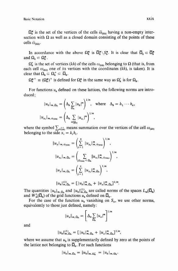
ot is the set of the vertices of the cells W(kh) having a non-empty inter­section with 0 as well as a closed domain consisting of the points of these cells W(kh)'

In accordance with the above nt is 0t\st. It is clear that Oh c 0: and nh en:.

ot is the set of vertices (kh) of the cells W(kh) belonging to n (that is, from each cell W(kh) one of its vertices with the coordinates (kh), is taken). It is clear that nh c n: c 0h'

n:+ == (n:)+ is defined for n: in the same way as nt is for nh •

For functions Un defined on these lattices, the following norms are intro­duced;

Iluhllm,nh = (.1h ~ Iuhlm rim, where

Iluxillm,WCkh) = (.1h L IUXilm)l/m, "'f~>")

where the symbol L"'l~~) means summation over the vertices of the cell W(kh)

belonging to the side Xi = ki hi'

Iluxllm,WCkh) = (tl IIUXill:::,WCkh)r /m,

Iluhll~,)nh = [lluhll:::,nh + Iluxll:::,nhJl/m. The quantities Iluhllm,nh and Iluhll~,)nh are called norms of the spaces Lm(Oh) and W~(nh) of the grid functions Uh defined on 0h'

For the case of the function Uh vanishing on Sh' we use other norms, equivalently to those just defined, namely:

and

Iluhll~.>cih = [lluhll:::,nh + Iluxll:::,nhJ1/m, where we assume that Uh is supplementarily defined by zero at the points of the lattice not belonging to Oh' For such functions

Iluhllm,nh = Iluhllm,n~ = Iluhllm,nh'

xxx Basic Notation

The symbol I Ux I means yfu! and u; = L7 = 1 U;i' where U;i = (u,y. Analogously U;iXj is (UXiX/. In writing difference quotients UXi ' UXiXj ' •••

for the grid function Uh the index "h" is omitted.

At the beginning of §3, Chapter VI, several interpolations of the grid functions Uh defined on Oh are introduced, namely: ul·) (or Uh) is a piecewise constant function equal for x E W(kh) to the value Uh at the vertex (kh); u~O (or u~) is a continuous piecewise smooth function on Oh poly linear on every W(kh) and equal to Uh at all (kh) E 0h.

u(m)(·) (or u(m») is a function that within each cell W(kh) is constant over Xm

and on the side Xm = km hm' Uh is interpolated by the principle of ( )~ described in the preceding sentence.

The symbol (u:;)(.) (or ux ) denotes interpolation of the first type of the grid function U Xi which is a difference quotient for the lattice function Uh.

In non-stationary problems the time variable t plays a special role. In them, the step of t in place of hn + 1 is denoted by r and the symbol Uh'

h = (hi' ... ' hn+ 1), is replaced by Uj..

It is assumed throughout the book that the coefficients aij' i,j = 1, ... , n,

of equations' terms involving derivatives of second order form a symmetric matrix; that is, aij = aji.