applied mathematical modelling - yazd · in view of the convergence of the method, some...

Applied Mathematical Modelling 37 (2013) 3917–3928

Contents lists available at SciVerse ScienceDirect

Applied Mathematical Modelling

journal homepage: www.elsevier .com/locate /apm

Application of variational iteration method for Hamilton–Jacobi–Bellmanequations

B. Kafash a,⇑, A. Delavarkhalafi a, S.M. Karbassi b

a Faculty of Mathematics, Yazd University, Yazd, P.O. Box 89197/741, Iranb Faculty of Advanced Education, Islamic Azad University, Yazd Branch, Yazd, P.O. Box 89195/155, Iran

a r t i c l e i n f o a b s t r a c t

Article history:Received 31 January 2012Received in revised form 1 July 2012Accepted 17 August 2012Available online 30 August 2012

Keywords:Optimal control problemsHamilton–Jacobi–Bellman (HJB) EquationsVariational iteration method (VIM)Banach’s fixed point theorem

0307-904X/$ - see front matter � 2012 Elsevier Inchttp://dx.doi.org/10.1016/j.apm.2012.08.013

⇑ Corresponding author.E-mail addresses: [email protected], Bka

In this paper, we use the variational iteration method (VIM) for optimal control problems.First, optimal control problems are transferred to Hamilton–Jacobi–Bellman (HJB) equationas a nonlinear first order hyperbolic partial differential equation. Then, the basic VIM isapplied to construct a nonlinear optimal feedback control law. By this method, the controland state variables can be approximated as a function of time. Also, the numerical value ofthe performance index is obtained readily. In view of the convergence of the method, someillustrative examples are presented to show the efficiency and reliability of the presentedmethod.

� 2012 Elsevier Inc. All rights reserved.

1. Introduction and preliminaries

Optimal control is a mathematically challenging and practically significant discipline. It is used in different fields such asengineering, economics and finance. In practice, many optimal control problems are subject to constraints in the state and/orcontrol variables. The optimal control problem has been studied in many textbooks [1–10] and by many researchers [11–13].In describing a control model, the kind of information available to the controller at each instant of time plays an importantrole. Several situations are possible [4]:

1. The controller has no information during the system operation. Such controls are often called optimal open loop control.2. The controller knows the state of the system at each instant of time t. Such controls are called optimal feedback control.

The goal of optimal control is to determine one of these presented controls to satisfy the system physical constraints andat the same time to minimize or maximize a performance index. Bellman’s dynamic programming method (Hamilton–Jacobi–Bellman) and Pontryagin’s maximum principle method [1–13] represent the most known methods for solving optimal controlproblems. HJB equation is a nonlinear first order hyperbolic partial differential equation which is used for constructing anonlinear optimal feedback control law. The HJB equation has not analytical solution in general, thus finding a numericalsolution is at least the most logical way to treat them. The study of numerical methods has provided an attractive fieldfor researchers of mathematical sciences which has risen to the appearance of different numerical computational methodsand efficient algorithms to solve the optimal control problems; for details, see [14–18]. Vlassenbroeck has presented anumerical technique for solving nonlinear constrained optimal control problems [19]. Jaddu has presented numerical meth-ods to solve unconstrained and constrained optimal control problems [20,21]. In [22], the authors have presented a spectral

. All rights reserved.

[email protected] (B. Kafash).

http://dx.doi.org/10.1016/j.apm.2012.08.013

mailto:[email protected]

mailto:[email protected]


http://www.sciencedirect.com/science/journal/0307904X

http://www.elsevier.com/locate/apm

3918 B. Kafash et al. / Applied Mathematical Modelling 37 (2013) 3917–3928

method of solving the controlled Duffing oscillator. In [23], a numerical technique is shown for solving the controlled Duffingoscillator; in which the control and state variables are approximated by Chebyshev series. In [24,25], some algorithms arepresented for solving optimal control problems and the controlled Duffing oscillator. Fakharian et al. have solved the optimalcontrol using Adomian decomposition method [26]. In [27,28], the authors have used homotopy perturbation method tosolve HJB equations. In recent years, viscosity solution as a new notion of solution is introduced [5]. Huang et al. have pro-posed a semi-meshless discretization method for the approximation of viscosity solutions to a first order HJB equation [29].An optimal control software package, MISER3, has been developed by Jennings et al. [30,31] to solve the optimal controlproblems. MISER3 has been used in solving various kinds of control problems in different aspects [32].

The VIM has been proposed by He [33–41]. This method is used to solve various kinds of functional equations. In fact, byimplementing this method a large class of nonlinear problems converge rapidly to approximate solutions. The method cansolve various different nonlinear equations [42–44]. The VIM is used in [45] to solve some problems in calculus of variations.In [46], VIM was used for finding the optimal control for linear quadratic problems. Recently, Berkani et al. reformulated theoptimal control problem as a variational problem and have use the VIM to solve the Euler–Lagrange equation correspondingto the formulated variational problem [47].

This paper is organized into following sections of which this introduction is the first. In Section 2, we introduce problemstatement. Section 3 is about dynamic programming; Hamilton–Jacobi–Bellman Equation. Variational iteration method isdescribed in Section 4. Section 5 derives the method. Convergence analysis is described in Section 6. In Section 7 we presentsome numerical examples to illustrate the efficiency and reliability of the presented method. Finally, the paper is concludedwith conclusion.

2. Problem statement

Consider a process described by the following system of nonlinear differential equations, which is called the equation ofmotion, on a fixed interval ½t0; t1�

_x ¼ f ðt; xðtÞ;uðtÞÞ; ð1Þ

where x 2 Rn is the state vector. Let U � Rm be a closed set. A piecewise continuous function u : ½t0; t1� ! Rm is said to be anadmissible control if uðtÞ 2 U. Let U be the class of such admissible controls. The function f : R1 � Rn � Rm ! Rn is a vectorfunction which is continuous and has continuous first partial derivative with respect to x. The initial condition for (1) is

xðt0Þ ¼ x0; ð2Þ

where x0 is a given vector in Rn. For each uðtÞ 2 U , let xðtÞ be the corresponding vector-value function which satisfies thedifferential equation (1) on interval ½t0; t1� and the initial condition (2). This function is called the trajectory correspondingto the control uðtÞ and initial condition x0. The value of xðtÞ at time t is called the state of the system at time t.

Along with this controlled process, we have a cost functional of the form

Jðx0;uÞ ¼ /ðt1; xðt1ÞÞ þZ t1

t0

Lðt; xðtÞ;uðtÞÞdt: ð3Þ

Here, Lðt; x; uÞ is the running cost, and /ðt; xÞ is the terminal cost. This cost functional depends on the initial position ðt0; x0Þand the choice of control uð�Þ. The optimization problem is therefore to minimize Jðx0;uÞ, for each ðx0;uÞ, over all controlsuðtÞ 2 U. The pair ðx0;uÞ which achieves this minimum is called an optimal control. In fact, the optimization problem withperformance index as in Eq. (3) is called a Bolza problem. There are two other equivalent optimization problems, whichare called Lagrange and Mayer problems [4].

3. Dynamic programming: Hamilton–Jacobi–Bellman equation

The use of the principle of optimality, usually known as dynamic programming, to derive an equation for solving optimalcontrol problem, was first proposed by Bellman [1] and Bellman and Dreyfus [1,2]. In dynamic programming a family of fixedinitial point controls problem is considered. The minimum value of the performance index is considered as a function of thisinitial point. This function is called the value function. Whenever the value function is differentiable, it satisfies a nonlinearfirst order hyperbolic partial differential equation called the partial differential equation of dynamic programming. Thisequation is used for constructing a nonlinear optimal feedback control law. If we consider a family of optimization problemswith differential initial condition ðt; xÞ, we consider the dependence of the value of these optimization problems on their ini-tial conditions. Thus a value functions is defined by

Vðt; xÞ ¼ infu2U

/ðt1; xðt1ÞÞ þZ t1

tLðs; xðsÞ;uðsÞÞds

� �¼ Jðx;u�Þ:

The next theorem shows that, at points at which the value function is well behaved, the partial differential inequalities orequations hold.

B. Kafash et al. / Applied Mathematical Modelling 37 (2013) 3917–3928 3919

Theorem 1 (See [4]). Let ðt; xÞ be any interior point of the set fðt; xÞ 2 Rnþ1jU – ;g at which the function Vðt; xÞ is differentiable.Function Vðt; xÞ satisfies the partial differential inequality

Vt þ Vxf ðt; x;vÞ þ Lðt; x; vÞP 0

for all v 2 U. If there is an optimal control u� 2 U, then the partial differential equation

Vt þminv2U

Vxf ðt; x;vÞ þ Lðt; x;vÞf g ¼ 0 ð4Þ

is satisfied.The partial differential equation (4) is called the partial differential equation of dynamic programming, which satisfies the

boundary condition

Vðt1; xðt1ÞÞ ¼ /ðt1; xðt1ÞÞ:

By introducing the Hamiltonian function

Hðt; x;v ;VxÞ ¼ Vxf ðt; x; vÞ þ Lðt; x;vÞ;

we have

Vt þminv2U

Hðt; x;v ;VxÞ ¼ 0: ð5Þ

Minimization of (5) leads to the expression for control law u�, as a function of t; xðtÞ and Vx defined by

u� ¼ wðt; x;VxÞ: ð6Þ

This leads to a Hamilton–Jacobi–Bellman equation with the boundary condition as

ðHJBÞVt þ Hðt; x;u�;VxÞ ¼ 0;Vðt1; xðt1ÞÞ ¼ /ðt1; xðt1ÞÞ:

�

4. Variational iteration method

In this section, the VIM is discussed. The VIM has been receiving much attention in recent years in applied mathematics ingeneral, and in the area of series solutions in particular. VIM is a well-known mathematical method, established by He [34–42], is thoroughly used by mathematicians to handle a wide variety of scientific and engineering applications. The methodgives the solution in the form of a rapidly convergent successive approximations that may give the exact solution if such asolution exists. For concrete problems where exact solution is not obtainable, it is found that a few number of approxima-tions can be used for numerical purposes. In fact, the VIM demonstrates fast convergence of the solution and therefore pro-vides several significant advantages [48]. The Adomian decomposition method suffers from the cumbersome work neededfor the derivation of Adomian polynomials for nonlinear terms. The homotopy perturbation method suffers from the com-putational work specially when the degree of nonlinearity increases. The numerical techniques, such as Galerkin method,also suffer from the need of huge size of computational work [49]. The VIM has no specific requirements for nonlinear oper-ators. To illustrate the basic concept of the technique, the main steps of the method are briefly described. Consider the fol-lowing general differential equation

Luþ Nu ¼ gðxÞ; ð7Þ

where L and N are linear and nonlinear operators, respectively, and gðxÞ is the source inhomogeneous term. In [34–42], Heproposed the variational iteration method is which a correction functional for Eq. (7) can be written as

unþ1ðtÞ ¼ unðtÞ þZ t

0kðnÞ LunðnÞ þ N~unðnÞ � gðnÞð Þdn; ð8Þ

where k is a general Lagrange multiplier, which can be identified optimally via the variational theory, and ~un is a restrictedvariation which means d~un ¼ 0.

The Lagrange multiplier is determined optimally with integration by parts. In other words we can use
ZkðnÞu0nðnÞdn ¼ kðnÞunðnÞ �
Zk0ðnÞunðnÞdn;

ZkðnÞu00nðnÞdn ¼ kðnÞu0nðnÞ � k0ðnÞunðnÞ þ

Zk00ðnÞunðnÞdn

and so on. The last two identities can be obtained by integrating by parts.The successive approximations unþ1ðtÞ; n P 0, of the solution uðtÞ will be readily obtained upon using the Lagrangian

multiplier determined and any selective function u0ðtÞ. In fact, the correction functional (8) will give several approximations,


and therefore the exact solution is obtained as the limit of the resulting successive approximations. So, the solution is givenby

u ¼ limn!1

un:

5. Deriving the method

In this section we describe the application of VIM for solving HJB equations. As mentioned before, the optimal controlproblems (1)–(3) lead to a HJB equation in Vðt; xÞ with the boundary condition as follows

ðHJBÞ@V@t þ

@Vðt;xÞ@x f ðt; xðtÞ;wÞ þ Lðt; xðtÞ;wÞ ¼ 0;

Vðt1; xðt1ÞÞ ¼ /ðt1; xðt1ÞÞ:

(ð9Þ

This equation is a sufficient condition for optimality. In general it is not possible to solve this equation analytically [20], thusfinding an approximate solution is at least the most logical way to solve them. Here numerical methods, one of which is theVIM method, are applied. The VIM admits the use of the correction functional for Eq. (9) which can be written as

Vnþ1ðt; xÞ ¼ Vnðt; xÞ þZ t1

tkðnÞ @Vnðn; xÞ

@nþ @

eV nðn; xÞ@x

f ðn; x;wÞ þ Lðn; x;wÞ !

dn; ð10Þ

where k is the Lagrange multiplier; here it may be a constant or a function, and eV n is a restricted value with deV n ¼ 0. Takingthe variation of both sides of (10) with respect to the independent variable Vn we find

dVnþ1

dVn¼ 1þ d

dVn

Z t1

tkðnÞ @Vnðn; xÞ

@nþ @

eV nðn; xÞ@x


dn;

or equivalently

dVnþ1ðt; xÞ ¼ dVnðt; xÞ þ dZ t1

tkðnÞ @Vnðn; xÞ

@nþ @

eV nðn; xÞ@x


dn

!;

that gives

dVnþ1ðt; xÞ ¼ dVnðt; xÞ þ dZ t1

tkðnÞ @Vnðn; xÞ

@ndn

� �; ð11Þ

obtained upon using deV n ¼ 0 and dL ¼ 0. Integrating the integral of (11) by parts we obtain

dVnþ1 ¼ dVn þ d kðnÞVnðn; xÞjn¼t1n¼t

� �� d

Z t1

tk0ðnÞVnðn; xÞdn

� �;

or equivalently

dVnþ1 ¼ d 1� kðnÞjn¼t

� Vn � d

Z t1

tk0ðnÞVnðn; xÞdn

� �: ð12Þ

The extremum condition of Vnþ1 requires that dVnþ1 ¼ 0. This means that the left hand side of (12) is 0, and as a result theright hand side should be 0 as well. This yields the stationary conditions

1� kjn¼t ¼ 0;

� k0jn¼t ¼ 0:

This in turn gives

k ¼ 1:

Substituting this value of the Lagrange multiplier into the functional (10) gives the iteration formula

Vnþ1ðt; xÞ ¼ Vnðt; xÞ þZ t1

t

@Vnðn; xÞ@n

þ @Vnðn; xÞ@x

f ðn; x;wÞ þ Lðn; x;wÞ� �

dn; ð13Þ

obtained upon deleting the restriction on Vn that was used for the determination of k. Considering the given conditionVðt1; xðt1ÞÞ ¼ /ðt1; xðt1ÞÞ, we can select the zeroth approximation V0ðt; xÞ ¼ /ðt; xðtÞÞ. The successive approximationsVnþ1ðt; xÞ; n P 0 of the solution Vðt; xÞ will be obtained readily upon using the obtained Lagrange multiplier and by usingany selective function V0. So, the correction functional (13) will give several approximations, and therefore the exact solutionis obtained as the limit of the resulting successive approximations. In fact, the solution is given by


Vðt; xÞ ¼ limn!1

Vnðt; xÞ:

The above result is summarized in the following algorithm. The main idea of this algorithm is to transform the optimalcontrol problems (1)–(3) into a HJB Eq. (9) and then solve this partial differential equation using the variational iterationmethod.

Algorithm 1.

Input: Optimal control problem (1)–(3). A tolerance � > 0 for accuracy of the solution and initial approximationV0ðt; xÞ.

Output: An optimal value for performance index J.
Step 1. Minimize Hamilton function Hðt; x;v ;VxÞ to derive control law of the form 6. Step 2. Let n ¼ 0, from V0ðt; xÞ compute optimal control u and corresponding trajectory x and J0. Step 3. Derive the HJB equation corresponding to optimal control problems (1)–(3). Step 4. n! nþ 1, solve the nonlinear equation (9) using the variational iteration method to obtain the value function
Vðt; xÞ and substitute this expression in (6) to obtain the optimal control law.
Step 5. Substitute u�ðtÞ in Step 4 in (1) with initial condition (2) to obtain the optimal trajectory x�ðtÞ and find Jn. Step 6. If jJn�1 � Jnj < � then set J ¼ Jn and stop, otherwise return to Step 4.
6. Convergence analysis

This section covers the convergence analysis of the proposed method. As a well-known powerful tool, for convergence ofthe VIM we have the following theorem [50–52]:

Theorem 2 (Banach’s fixed point theorem [53]). Assume that K is a non-empty closed set in a Banach space V, and further, thatT : K ! K is a contractive mapping with contractively constant a; 0 6 a < 1. Then the following results hold.

1. There exists a unique u 2 K such that u ¼ T ðuÞ.2. For any u0 2 K, the sequence fung � K defined by unþ1 ¼ T ðunÞ; n ¼ 0;1; . . ., converges to u.

According to above Theorem, for the nonlinear mapping

T ½V � ¼ Vnðt; xÞ þZ t

t1

@Vnðn; xÞ@n

þ @Vnðn; xÞ@x


dn; ð14Þ

the sequence (14) converges to the fixed point of T which is also the solution of Hamilton–Jacobi–Bellman equation if oper-ator T is strictly contractive. To investigate the convergence of Algorithm 1, we have used the same approach as in [51]. Now,define the operator A½V � as,

A½V � ¼Z t

t1

@Vnðn; xÞ@n

þ @Vnðn; xÞ@x


dn ð15Þ

and define the components vk; k ¼ 0;1;2; . . ., as,

v0 ¼ V0;

v1 ¼ A½v0�;v2 ¼ A½v0 þ v1�;...

vkþ1 ¼ A½v0 þ v1 þ � � �vn�:

8>>>>>>><>>>>>>>:ð16Þ

Then we have Vðt; xÞ ¼ limn!1Vnðt; xÞ ¼P1

k¼0vkðt; xÞ. Therefore, as a result, the solution of problem (9) can be derived, using(15) and (16), in the series form,

Vðt; xÞ ¼X1k¼0

vkðt; xÞ: ð17Þ

For the approximation purpose, we approximate the solution Vðt; xÞ by the nth order truncated seriesPn

k¼0vkðt; xÞ.Next theorem is a special case of Banach’s fixed point theorem which is used in [50], as a sufficient condition, to study the

convergence of VIM for some partial differential equations [51].


Theorem 3 (See [51]). Let A, defined in (15), be an operator from a Hilbert space H to H. The series solutionVðt; xÞ ¼

P1k¼0vkðt; xÞ, defined in (17), converges if 90 < c < 1 such that kvkþ1k 6 ckvkk; 8k 2 N [ f0g.

Theorem 4 (See [51]). If the series solution Vðt; xÞ ¼P1

k¼0vkðt; xÞ, defined in (17), converges then it is an exact solution of thenonlinear problem (9).

In summary, Theorems 3 and 4 state that the variational iteration solution of nonlinear problem (9), obtained using theiteration formula (13) or (16), converges to an exact solution under the condition that 90 < c < 1 such thatkvkþ1k 6 ckvkk; 8k 2 N [ f0g. In other words, if we define, for every i 2 N [ f0g, the parameters,

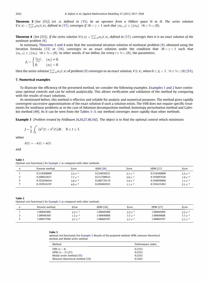
Table 1Optima

n

1357

Table 2Optima

n

135

bi ¼kv iþ1kkv ik

; kv ik – 0;

0; kv ik ¼ 0

(
then the series solution
P1k¼0vkðt; xÞ of problem (9) converges to an exact solution, Vðt; xÞ, when 0 6 bi < 1; 8i 2 N [ f0g [51].

7. Numerical examples

To illustrate the efficiency of the presented method, we consider the following examples. Examples 1 and 2 have contin-uous optimal controls and can be solved analytically. This allows verification and validation of the method by comparingwith the results of exact solutions.

As mentioned before, this method is effective and reliable for analytic and numerical purposes. The method gives rapidlyconvergent successive approximations of the exact solution if such a solution exists. The VIM does not require specific treat-ments for nonlinear problems as in the case of Adomian decomposition method, homotopy perturbation method and Galer-kin method [49]. As it can be seen from the Tables 1–3, our method converges more rapidly than other methods.

Example 1 (Problem treated by Feldbaum [4,24,27,46,54]). The object is to find the optimal control which minimizes

J ¼ 12

Z 1

0u2ðtÞ þ x2ðtÞ�

dt; 0 6 t 6 1;

when

_xðtÞ ¼ �xðtÞ þ uðtÞ

and

l cost functional J for Example 1 as compared with other methods.

Present method Error ADM [26] Error HPM [27] Error

0.218360008 2.5 e�2 0.224030251 3.1 e�2 0.218360008 2.5 e�2

0.200652631 7.7 e�3 0.212708623 2.0 e�2 0.193097636 1.9 e�4

0.193294416 3.8 e�4 0.206778119 1.4 e�2 0.194059806 1.1 e�3

0.192914197 4.9 e�6 0.203602923 1.1 e�2 0.193415452 5.1 e�4

l cost functional J for Example 2 as compared with other methods.

Present method Error ADM [26] Error HPM [27] Error

1.06845960 2.2 e�2 1.06845960 2.2 e�2 1.06845960 2.2 e�2

1.08949369 1.3 e�3 1.09849888 7.7 e�3 1.09849888 7.7 e�3

1.09075706 2.7 e�5 1.08869787 2.1 e�3 1.08869787 2.1 e�3

Table 3optimal cost functional J for Example 3. Results of the proposed method, HPM, measure theoreticalmethod and Modal series method.

Method Performance index

VIM (n ¼ 4) 0.2353HPM (n ¼ 5) [27] 0.2353Modal series method [55] 0.2353Measure theoretical method [10] 0.2425


xð0Þ ¼ 1

are satisfied. We can obtain the analytical solution by the use of Pontryagin’s maximum principle which is [24]:

xðtÞ ¼ Aeffiffi2p

t þ ð1� AÞe�ffiffi2p

t ;

uðtÞ ¼ Aðffiffiffi2pþ 1Þe

ffiffi2p

t � ð1� AÞðffiffiffi2p� 1Þe�

ffiffi2p

t

and

J ¼ e�2ffiffi2p

2ðffiffiffi2pþ 1Þðe4

ffiffi2p� 1ÞA2 þ ð

ffiffiffi2p� 1Þðe2

ffiffi2p� 1Þð1� AÞ2

� �;

where

A ¼ 2ffiffiffi2p� 3

�e2ffiffi2pþ 2

ffiffiffi2p� 3

:

The dynamic programming equation (4) has the form for this case

@V@tþmin

uðtÞ

@V@x�xðtÞ þ uðtÞð Þ þ 1

2u2ðtÞ þ 1

2x2ðtÞ

� �¼ 0 ð18Þ

and the boundary condition is

Vð1; xð1ÞÞ ¼ 0:

The corresponding Hamiltonian function is

Hðt; x;u;VxÞ ¼@V@x�xðtÞ þ uðtÞð Þ þ 1

2u2ðtÞ þ 1

2x2ðtÞ:

To obtain a solution for (18), we proceed in two steps. The firs step is to perform the indicated minimization as follow

@H@u¼ uðtÞ þ @V

@x;

that leads to a control law of the form

u� ¼ � @V@x

:

Because @2H@u2 ¼ 1 > 0; u� is minimum and acceptable. Now, by substituting u� in HJB equation, we have the following equa-

tion with the boundary condition:

ðHJBÞ@V@t þ 1

2 x2 � x @Vðt;xÞ@x � 1

2 ð@Vðt;xÞ@x Þ

2 ¼ 0;Vð1; xð1ÞÞ ¼ 0:

(ð19Þ

Now we solve this nonlinear partial differential equation using VIM. The correction functional for this equation reads

Vnþ1ðt; xÞ ¼ Vnðt; xÞ þZ t

1kðnÞ @Vnðn; xÞ

@nþ 1

2x2 � x

@ eV nðn; xÞ@x

� 12

@ eV nðn; xÞ@x

!20@ 1Adn: ð20Þ

The stationary conditions

1� kjn¼t ¼ 0;

� k0jn¼t ¼ 0;

give

k ¼ 1:

Substituting this value of the Lagrange multiplier into the functional (20) gives the iteration formula for n P 0

Vnþ1ðt; xÞ ¼ Vnðt; xÞ þZ t

1

@Vnðn; xÞ@n

þ 12

x2 � x@Vnðn; xÞ

@x� 1

2@Vnðn; xÞ

@x

� �2 !

dn:

Selecting V0ðt; xÞ ¼ 0 from the given initial condition yields the successive approximations


V0ðt; xÞ ¼ 0;

V1ðt; xÞ ¼ �12ðt � 1Þx2;

V2ðt; xÞ ¼16

t3 � 6t2 þ 6t � 1�

x2;

V3ðt; xÞ ¼1

126t7 � 1

9t6 þ 8

15t5 � 17

18t4 þ 2

9t3 þ 2

3t2 � 7

9t þ 127

315

� �x2;

..

.

Now, by computing bi’s for this problem, we have,

b0 ¼ 0;b1 ¼ kv2k

kv1k¼ 0:990430406;

b2 ¼ kv3kkv2k¼ 0:734218978;

b3 ¼ kv4kkv3k¼ 0:531347665;

b4 ¼ kv5kkv4k¼ 0:486441525;

..

.

8>>>>>>>>>>>><>>>>>>>>>>>>:
Here, bi’s are less than one, for i P 1 and 0 6 t 6 1. This confirms that the variational approach for nonlinear equation (19)converges to exact solution. We can calculate state and control variables approximately after choosing of an approximationfor Vðt; xÞ. The obtained solutions and the analytical solution are plotted in Fig. 2 for different n.
The exact solution for the performance index is J ¼ 0:192909295. Comparison of the VIM of the optimal cost functional Jwith other methods are shown in Table 1.

Example 2. The object is to find the optimal control which minimizes

J ¼ 12

Z 1

0u2ðtÞdt þ x2ð1Þ;

when

_xðtÞ ¼ xðtÞ þ uðtÞ

and

xð0Þ ¼ 1

are satisfied [3,27]. We can obtain the analytical solution by the use of Pontryagin’s maximum principle which is:

xðtÞ ¼ A1þ 2e2t�2ffiffiffiffiffiffiffiffiffiffiffiffiffiffi

2t � 2p

� �;

uðtÞ ¼ �A2ffiffiffiffiffiffiffiffiffiffiffiffiffiffi

2t � 2p� �

;

where

A ¼ ee2 þ 1

:

The corresponding Hamiltonian function is

Hðt; x;u;VxÞ ¼@V@x

xðtÞ þ uðtÞð Þ þ u2ðtÞ:

For obtaining optimal control, we calculate @H@u as follow

@H@u¼ 2uðtÞ þ @V

@x¼ 0;

therefore,

u�ðtÞ ¼ �12@V@x

:

Because @2H@u2 ¼ 2 > 0;u� is minimum and acceptable. Now, by substituting u� in HJB equation, we have the following equa-

tion with the boundary condition:

0

0

0

0

0

0

0

0

x (t)


ðHJBÞ@V@t þ x @Vðt;xÞ

@x � 14 ð

@Vðt;xÞ@x Þ

2 ¼ 0;Vð1; xð1ÞÞ ¼ x2ð1Þ:

(ð21Þ

Now we solve this nonlinear partial differential equation using VIM. The correction functional for this equation reads

Vnþ1ðt; xÞ ¼ Vnðt; xÞ þZ 1

tkðnÞ @Vnðn; xÞ

@nþ x

@ eV nðn; xÞ@x

� 14

@ eV nðn; xÞ@x

!20@ 1Adn: ð22Þ

The stationary conditions lead to the Lagrange multiplier k ¼ 1. Substituting this value of the Lagrange multiplier into thefunctional (22) gives the iteration formula for n P 0


t

@Vnðn; xÞ@n

þ x@Vnðn; xÞ

@x� 1

4@Vnðn; xÞ

@x

� �2 !

dn:

Selecting V0ðt; xÞ ¼ x2 from the given initial condition yields the successive approximations

V0ðt; xÞ ¼ x2;

V1ðt; xÞ ¼ �ðt � 2Þx2;

V2ðt; xÞ ¼13

t3 � t2 þ 53

� �x2;

V3ðt; xÞ ¼1

63t7 � 1

9t6 þ 1

5t5 þ 1

9t4 � 4

9t3 � 5

9t þ 562

315

� �x2;

..

.

Now, by computing bi’s for this problem, we have,

b0 ¼ kv1kkv0k¼ 0:218217890;

b1 ¼ kv2kkv1k¼ 0:286990527;

b2 ¼ kv3kkv2k¼ 0:200667823;

b3 ¼ kv4kkv3k¼ 0:169595191;

b4 ¼ kv5kkv4k¼ 0:141191454;

..

.

8>>>>>>>>>>>>><>>>>>>>>>>>>>::

Here, bi’s are also less than one, for i P 0 and 0 6 t 6 1. This confirms that the variational approach for nonlinear equation(21) converges to exact solution. We can calculate state and control variables approximately after choosing of an approxi-mation for Vðt; xÞ. The obtained solutions and the analytical solution are plotted in Fig. 1 for different n.

The exact solution for the performance index is J ¼ 1:09078425. Comparison of the VIM of the optimal cost functional Jwith other methods are shown in Table 1.

Example 3. Consider the following problem [10,27,55]:Minimize

0 0.1 0.2 0.3 0.4 0.5 0.6 0.7 0.8 0.9 1.2

.3

.4

.5

.6

.7

.8

.9

1

t

x1(t)x3(t)x5(t)Exact Solution

0 0.1 0.2 0.3 0.4 0.5 0.6 0.7 0.8 0.9 1−0.9

−0.8

−0.7

−0.6

−0.5

−0.4

−0.3

−0.2

−0.1

0

0.1

t

u (t)

u1(x)

u3(x)

u5(t)

Exact Solution

Fig. 1. Solution of Example 1. The approximate solution for different n as compared with the actual analytical solution.

0

0

0

0

x (t)


J ¼Z 1

0U2ðsÞds

for s 2 ½0;1� subject to

_XðsÞ ¼ 12

X2ðsÞ sinðXðsÞÞ þ UðsÞ;

Xð0Þ ¼ 0; Xð1Þ ¼ 12: ð23Þ

First, we use the transformation s ¼ �t. Therefore, the corresponding Hamiltonian function for t 2 ½�1;0� will be:

Hðt; x;u;VxÞ ¼ u2ðtÞ � @V@x

12

x2ðtÞ sinðxðtÞÞ þ uðtÞ� �

:

For obtaining optimal control, we calculate @H@u as follow

@H@u¼ 2uðtÞ � @V

@x¼ 0:

Therefore,

u�ðtÞ ¼ 12@V@x

:

Because @2H@u2 ¼ 2 > 0; u� is minimum and acceptable. Now, by substituting u� in HJB equation, following equation with the

boundary condition is obtained:

ðHJBÞ@V@t � 1

2@Vðt;xÞ@x x2 sinðxÞ � 1

4@Vðt;xÞ@x

� �2¼ 0;

Vð0; xð0ÞÞ ¼ 0:

8<: ð24Þ

The correction functional for this equation leads to the iteration formula


t

@Vnðn; xÞ@n

� 12@Vnðn; xÞ

@xx2 sinðxÞ � 1

4@Vnðn; xÞ

@x

� �2 !

dn:

Selecting V0ðt; xÞ ¼ x from the given initial condition yields the successive approximations, with bi’s for this problem as

b0 ¼ kv1kkv0k¼ 0:359481844;

b1 ¼ kv2kkv1k¼ 0:505731484;

b2 ¼ kv3kkv2k¼ 0:450598088;

..

.

8>>>>>><>>>>>>:
Here, bi’s are also less than one, for i P 0 and �1 6 t 6 0. This confirms that the variational approach for nonlinear equation(24) converges to exact solution. Since u�ðtÞ ¼ 1
2@V@x , use of V4ðt; xÞ gives uðt; xÞ as a function of t and x. As XðsÞ ¼ s

2 is the opti-mal state trajectory [28,55]. By considering this optimal state trajectory, the optimal control UðsÞ ’ 1

2� 116 s

3 þ 41280 s

6 isachieved. This approximation solution is compared with the solutions from the HPM [27] and Modal series [55] (see Fig. 3.)

0 0.1 0.2 0.3 0.4 0.5 0.6 0.7 0.8 0.9 1

.65

0.7

.75

0.8

.85

0.9

.95

1

t

x1(t)x3(t)Exact Solution

0 0.1 0.2 0.3 0.4 0.5 0.6 0.7 0.8 0.9 1−2

−1.8

−1.6

−1.4

−1.2

−1

−0.8

−0.6

t

u (t)

u1(t)

u3(t)

Exact Solution

Fig. 2. Solution of Example 2. The approximate solution for different n as compared with the actual analytical solution.

0 0.1 0.2 0.3 0.4 0.5 0.6 0.7 0.8 0.9 10.43

0.44

0.45

0.46

0.47

0.48

0.49

0.5

τ

U (τ

)Modal SeriesHPMPresent Method

Fig. 3. Solution of Example 3. Comparison of the VIM control function and other methods.


Also, the approximate solution for the performance index obtained by the presented method, is compared with othermethod and results are listed in Table 1.

8. Conclusion

In this paper, variational iteration method was used to minimize the performance index of both linear and nonlinear opti-mal control problems. This method provides a simple way to adjust and obtain an optimal control which can easily be ap-plied to complex problems as well. One of the advantages of this method is its fast convergence. The obtained results are inconsonance with the results in [26] using Adomian decomposition method and the homotopy perturbation method [27,28].Adomian decomposition method suffers from the cumbersome work needed for the derivation of Adomian polynomials fornonlinear terms and the homotopy perturbation method suffers from the computational work specially when the degree ofnonlinearity increases. The merit of our method is that less computational effort it required because the recursive equationsobtained can be solved numerically using an appropriate initial approximation. Also, the numerical value of the performanceindex is obtained readily. Some examples were solved by this method, the results show that the presented method is morepowerful, giving more accurate results and hence reduce the computational costs significantly, which is an important factorto choose the method in engineering applications.

Acknowledgment

The authors wish to thank Mr M. Heydari for his useful comments.

Appendix A. Supplementary data

Supplementary data associated with this article can be found, in the online version, at http://dx.doi.org/10.1016/j.apm.2012.08.013.

References

[1] R.E. Bellman, Dynamic Programming, Princeton University Press, Princeton, NJ, 1957.[2] R.E. Bellman, S.E. Dreyfus, Applied Dynamic Programming, Princeton University Press, Princeton, NJ, 1962.[3] A.E. Bryson, Y.C. Ho, Applied Optimal Control, Hemisphere Publishing Corporation, Washangton, DC, 1975.[4] W.H. Fleming, C.J. Rishel, Deterministic and Stochastic Optimal Control, Springer Verlag, New York, 1975.[5] W.H. Fleming, H.M. Soner, Controlled Markov Processes and Viscosity Solutions, Springer, 2006.[6] D.E. Kirk, Optimal Control Theory An Introduction, Prentice-Hall, Englewood Cliffs, 1970.[7] A.B. Pantelev, A.C. Bortakovski, T.A. Letova, Some Issues and Examples in Optimal Control, MAI Press, Moscow, 1996 (in Russian).[8] E.R. Pinch, Optimal Control and the Calculus of Variations, Oxford University Press, London, 1993.[9] L.S. Pontryagin, The Mathematical Theory of Optimal Processes, Interscience, John Wiley and Sons, 1962.

[10] J.E. Rubio, Control and Optimization: The Linear Treatment of Non-linear Problems, Manchester University Press, Manchester, 1986.[11] M. Athans, The status of optimal control theory and application for deterministic systems, IEEE Trans. Autom. Control 11 (1699) 580–596.[12] A.E. Bryson, Optimal control – 1950 to 1985, IEEE Control Syst. Mag. 16 (1996) 26–33.[13] H.J. Sussmann, J.C. Willems, 300 years of optimal control: from the Brachystochrone to the maximum principle, IEEE Control Syst. Mag. 17 (1997) 32–

44.[14] N.U. Ahmed, Elements of Finite-Dimensional Systems and Control Theory, Longman Scientific and Technical, England, 1988.[15] B.D. Craven, Control and Optimization, Chapman and Hall, London, 1995.[16] A. Miele, Gradient algorithms for the optimization of dynamic systems, Control and Dynamic Systems: Advances in Theory and Applications, vol. 16,

Academic Press, New York, 1980, pp. 1–52.[17] Y. Sakawa, Y. Shindo, On the global convergence of an algorithm for optimal control, IEEE Trans. Autom. Control AC-25 (1980) 1149–1153.




[18] K.L. Teo, K.H. Wong, A Unified Computational Approach to Optimal Control Problems, Longman Scientific and Technical, England, 1991.[19] J. Vlassenbroeck, A chebyshev polynomial method for optimal control with state constraints, Automatica 24 (4) (1988) 499–506.[20] H.M. Jaddu, Numerical Methods for Solving Optimal Control Problems Using Chebyshev Polynomials, Ph.D. Thesis, School of Information Science Japan,

Advanced Institute of Science and Technology, 1998.[21] H.M. Jaddu, Direct solution of nonlinear optimal control problems using quasilinearization and Chebyshev polynomials, J. Franklin Inst. 339 (2002)

479–498.[22] G.N. Elnagar, M. Razzaghi, A Chebyshev spectral method for the solution of nonlinear optimal control problems, Appl. Math. Model. 21 (5) (1997) 255–

260.[23] M. El-Kady, E.M.E. Elbarbary, A Chebyshev expansion method for solving nonlinear optimal control problems, Appl. Math. Comput. 129 (2002) 171–

182.[24] B. Kafash, A. Delavarkhalafi, S.M. Karbassi, Application of Chebyshev polynomials to derive efficient algorithms for the solution of optimal control

problems, Sci. Iran. D, Comput. Sci. Eng. Electr. Eng. 19 (3) (2012) 795–805.[25] B. Kafash, A. Delavarkhalafi, S.M. Karbassi, Numerical solution of nonlinear optimal control problems based on state parametrization, Iranian J. Sci.

Technol., in press.[26] A. Fakharian, M.T. Hamidi Beheshti, A. Davari, Solving the Hamilton–Jacobi–Bellman equation using Adomian decomposition method, Int. J. Comput.

Math. 87 (2010) 2769–2785.[27] H. Saberi Nik, S. Effati, M. Shirazian, An approximate-analytical solution for the Hamilton–Jacobi–Bellman equation via homotopy perturbation

method, Appl. Math. Model. 36 (2012) 5614–5623.[28] S. Effati, H. Saberi Nik, Solving a class of linear and nonlinear optimal control problems by homotopy perturbation method, IMA J. Math. Control Inform.

28 (4) (2011) 539–553.[29] C.S. Huanga, S. Wangb, C.S. Chenc, Z.C. Lia, Aradial basis collocation method for Hamilton–Jacobi–Bellman equations, Automatica 42 (2006) 2201–

2207.[30] L.S. Jennings, M.E. Fisher, K.L. Teo, C.J. Goh, MISER3 Optimal Control Software, Version 3: Theory and User Manual. <http://www.maths.uwa.edu.au/les/

miser3.3.html>.[31] L.S. Jennings, K.L. Teo, C.J. Goh, MISER3.2 Optimal Control Software: Theory and User Manual, Department of Mathematics, The University of Western

Australia, Australia, 1997. <http//www.cado.maths.uwa.edu.au>.[32] K.L. Teo, C.J. Goh, K.H. Wong, A Unified Computational Approach to Optimal Control Problems, Longman Scientific and Technical, London, 1991.[33] J.H. He, A new approach to nonlinear partial differential equations, Commun. Nonlinear Sci. Numer. Simul. 2 (4) (1997) 230–235.[34] J.H. He, Variational iteration method for delay differential equations, Commun. Nonlinear Sci. Numer. Simul. 2 (4) (1997) 235–236.[35] J.H. He, Approximate solution of nonlinear differential equations with convolution product nonlinearities, Comput. Methods Appl. Mech. Eng. 167

(1998) 69–73.[36] J.H. He, A variational iteration method – a kind of nonlinear analytical technique: some examples, Int. J. Nonlinear Mech. 34 (4) (1999) 699–708.[37] J.H. He, Approximate analytical solution for seepage flow with fractional derivatives in porous media, Comput. Methods Appl. Mech. Eng. 167 (1–2)

(1998) 57–68.[38] J.H. He, Approximate solution of nonlinear differential equations with convolution product nonlinearities, Comput. Methods Appl. Mech. Eng. 167 (1–

2) (1998) 69–73.[39] J.H. He, X.H. Wu, Construction of solitary solution and compaction-like solution by variational iteration method, Chaos Solitons Fract. 29 (1) (2006)

108–113.[40] J.H. He, Some asymptotic methods for strongly nonlinear equations, Int. J. Mod. Phys. B 20 (10) (2006) 1141–1199.[41] J.H. He, Variational iteration method for autonomous ordinary differential systems, Appl. Math. Comput. 114 (2–3) (2000) 115–123.[42] N. Bildik, A. Konuralp, The use of Variational iteration method differential transform methods and Adomian decomposition method for solving

different type of nonlinear partial differential equation, Int. J. Nonlinear Sci. Numer. Simul. 7 (2006) 65–70.[43] M. Dehghan, M. Tatari, Identifying and unknown function in parabolic equation with overspecified data via He’s VIM, Chaos Solitons Fract. 36 (2008)

157–166.[44] N.H. Sweilam, Variational iteration method for solving cubic nonlinear Schrodinger equation, J. Comput. Appl. Math. 207 (2007) 155–163.[45] M. Tatari, M. Dehghan, Solution of problems in calculus of variations via He’s variational iteration method, Phys. Lett. A 362 (2007) 401–406.[46] S.A. Yousefi, M. Dehghan, A. Lotfi, Finding the optimal control of linear systems via He-s variational iteration method, Int. J. Comput. Math. 87 (5)

(2010) 1042–1050.[47] S. Berkani, F. Manseur, A. Maidi, Optimal control based on the variational iteration method, Comput. Math. Appl., in press.[48] A.M. Wazwaz, Partial Differential Equations and Solitary Waves Theory, Springer, 2009.[49] A.M. Wazwaz, The variational iteration method for analytic treatment for linear and nonlinear ODEs, Appl. Math. Comput. 212 (2009) 120–134.[50] M. Tatari, M. Dehghan, On the convergence of He-s variational iteration method, J. Comput. Appl. Math. 207 (2007) 121–128.[51] Z.M. Odibat, A study on the convergence of variational iteration method, Math. Comput. Model. 51 (2010) 1181–1192.[52] F. Geng, A modified variational iteration method for solving Riccati differential equations, Comput. Math. Appl. 60 (2010) 1868–1872.[53] K. Atkinson, Theoretical Numerical Analysis, A Functional Analysis Framework, third ed., Springer, 2009.[54] T.M. El-Gindy, H.M. El-Hawary, M.S. Salim, M. El-Kady, A Chebyshev approximation for solving optimal control problems, Comput. Math. Appl. 29

(1995) 35–45.[55] A. Jajarmi, N. Pariz, A. Vahidian, S. Effati, A novel Modal series representation approach to solve a class of nonlinear optimal control problems, Int. J.

Innovative Comput. Inform. Control 7 (3) (2011) 1413–1425.

http://www.maths.uwa.edu.au/les/miser3.3.html

http://www.maths.uwa.edu.au/les/miser3.3.html

http://http//www.cado.maths.uwa.edu.au

applied mathematical modelling - yazd · in view of the convergence of the method, some...

Documents