applied mathematical modelling - swansea...

Applied Mathematical Modelling 34 (2010) 3917–3932

Contents lists available at ScienceDirect

Applied Mathematical Modelling

journal homepage: www.elsevier .com/locate /apm

High dimensional model representation for stochastic finiteelement analysis

R. Chowdhury *, S. AdhikariSchool of Engineering, Swansea University, Singleton Park, Swansea, SA2 8PP Wales, UK

a r t i c l e i n f o

Article history:Received 12 January 2009Received in revised form 31 March 2010Accepted 6 April 2010Available online 14 April 2010

Keywords:Function approximationHigh dimensional model representationKarhunen–Loève expansionRandom fieldStochastic finite element

0307-904X/$ - see front matter � 2010 Elsevier Incdoi:10.1016/j.apm.2010.04.004

* Corresponding author. Tel.: +44 (0)1792 602088E-mail address: [email protected] (R

a b s t r a c t

This paper presents a generic high dimensional model representation (HDMR) method forapproximating the system response in terms of functions of lower dimensions. The pro-posed approach, which has been previously applied for problems dealing only with randomvariables, is extended in this paper for problems in which physical properties exhibit spa-tial random variation and may be modelled as random fields. The formulation of theextended HDMR is similar to the spectral stochastic finite element method in the sensethat both of them utilize Karhunen–Loève expansion to represent the input, and lower-order expansion to represent the output. The method involves lower dimensional HDMRapproximation of the system response, response surface generation of HDMR componentfunctions, and Monte Carlo simulation. Each of the low order terms in HDMR is sub-dimen-sional, but they are not necessarily translating to low degree polynomials. It is an efficientformulation of the system response, if higher-order variable correlations are weak, allow-ing the physical model to be captured by the first few lower-order terms. Once the approx-imate form of the system response is defined, the failure probability can be obtained bystatistical simulation. The proposed approach decouples the finite element computationsand stochastic computations, and consecutively the finite element code can be treated asa black box, as in the case of a commercial software. Numerical examples are used to illus-trate the features of the extended HDMR and to compare its performance with full scalesimulation.

� 2010 Elsevier Inc. All rights reserved.

1. Introduction

Numerical methods for structural analysis have been developed quite substantially over the last decades. In particular,the finite element method (FEM) and closely related approximations have become state-of-the-art. The modelling capabil-ities and the solution possibilities lead to an increasing refinement allowing for more and more details to be captured in theanalysis. On the other hand, however, the need for more precise input data becomes urgent in order to avoid or reduce pos-sible modelling errors. Such errors could eventually render the entire analysis procedure useless. Typically, not all uncertain-ties encountered in structural analysis can be reduced by careful modelling since their source lies in the intrinsic randomness[1–3] of natural phenomena. It is therefore appropriate to utilize methods based on probability theory to assess such uncer-tainties and to quantify their effect on the outcome of structural analysis.

In the stochastic mechanics community, the need to account for uncertainties has long been recognized in order toachieve reliable design of structural and mechanical systems [4–6]. There is a general agreement that advanced computa-tional tools have to be employed to provide the necessary computational framework for describing structural response

. All rights reserved.

; fax: +44 (0)1792 295676.. Chowdhury).

http://dx.doi.org/10.1016/j.apm.2010.04.004

mailto:[email protected]

http://www.sciencedirect.com/science/journal/0307904X

http://www.elsevier.com/locate/apm

3918 R. Chowdhury, S. Adhikari / Applied Mathematical Modelling 34 (2010) 3917–3932

and reliability. A current popular method is the stochastic finite element method (SFEM) [7], which integrates probabilitytheory with standard FEM. Methods involving perturbation expansion [8], Neumann series expansion [9], first- and sec-ond-order reliability algorithms [10–12], and Monte Carlo simulation (MCS) [13] including variance reduction strategieshave been developed and extensively used for probabilistic analysis of complex structures. These developments includetreatment of spatially varying structural properties that are modelled as random fields, loads that are modelled as space–time random processes, structural behaviour covering static and dynamic regimes, linear and nonlinear structural/mechan-ical behaviour, characterization of response variability and determination of structural reliability measures. Early develop-ment of Spectral SFEM (SSFEM) by Ghanem and Spanos [7] appears to be a suitable technique for the solution of complex,general problems in probabilistic mechanics. However, this method requires access to the governing differential equations ofsystem. Furthermore, the resulting system of equations to be solved for the unknown response is much larger than thosefrom deterministic finite element analysis. For complicated large system problems, the system of equations in the SSFEMcould be tremendously large. For example, if the deterministic system is of size l � l, and the number of terms in the poly-nomial chaos expansion is p, then the size of the stochastic system would be p � l � p � l. Recently a new implementation ofSSFEM [14], which is theoretically equivalent to the original SSFEM, has been developed for the purpose of utilizing com-monly available FEM codes as a black box. This novel implementation of SSFEM uses random sampling of the input and con-sequently a large number of FEM runs to get a stable estimate of the coefficients in the expansion of the solution.

This paper presents a generic approach for solving random field problems arising in structural mechanics. The method-ology is based on high dimensional model representation (HDMR) which has been previously proposed by the authors [15–18] for problems dealing only with random variables. This paper extends HDMR concept to the problems involving randomfields. Proposed methodology uses Karhunen–Loève (K–L) expansion [19] for discretizing the input random field and HDMRto approximate the output response in terms of functions of lower dimensions as an efficient uncertainty propagation model.

Compared to the conventional surrogate models, present approach has several advantages to justify using it as a morereliable metamodel. The first is reduction of data processing. The exponentially growing amount of function values is rep-resented via polynomially growing tables [15,16] holding each function component (terms in the general expansion). Thisproperty helps us to cope with high dimensional problems of real world. The second advantage is reduction of computationalcomplexity. HDMR is generated by a family of (linear) projections [20,21]. Consequently, it allows splitting of any probleminto easier low-dimensional subproblems. Third advantage is that, HDMR is a mean square convergent series expansion. Thisis because of the inherent properties of orthogonal properties of HDMR component functions [20]. It is optimal in the Fouriersense since it minimizes the mean square error from truncation after a finite number of cooperative terms in the expansion.Also lower dimensional functions stay stable as higher order Taylor series terms are inherently included. Finally, comparedto existing simulation based random field approach [22], HDMR-based approach does not translate into lower-order poly-nomial approximation of system response. The formulation of the extended HDMR is similar to the SSFEM in the sense thatboth of them utilize K–L expansion to represent the input, and lower-order expansion to represent the output. The samplepoints in the proposed method are chosen from regularly spaced points along each of the variable axis. This sampling schemeresults in fewer system analysis [15,16].

Organization of the present paper is as follows. In Section 2, statement of the problem is set in the context of stochasticmechanics. Emphasis is put on explaining how to discretize the random field. Section 3 provides an overview of the theorybehind the implementation of HDMR. Section 4 describes the step-wise procedure of HDMR-based metamodel. In Section 5,computational steps of the proposed approach are discussed. Numerical examples are illustrated in Section 6, to show theperformance of the proposed approach.

2. Random field discretization

Let ðH;F ;PÞ be a probability space and let L2ðH;F ;PÞ be the Hilbert space of random variables with finite second mo-ments. A random fieldHðx; hÞwith x 2 RN and h 2 H, is curve in L2ðH;F ;PÞ, that is a collection of random variables indexedby x [23]. Hence, Hðx0; hÞ for a given x0 is a random variable and Hðx; h0Þ for a given h0 is a realization of the random field. AGaussian random field is such that for any N, the vector ½Hðx1; h0Þ; . . . ;HðxN; h0Þ�T is Gaussian. Moreover, it is homogeneous ifits mean lðx; h0Þ and variance r2ðx; h0Þ are constant and its autocorrelation coefficient qðx; x0Þ is a function of x and x0 only.This autocorrelation function may take many distinct forms. One such form is the exponential type

qðx; x0Þ ¼ e�a1 jxð1Þ�x0ð1Þ j�a2 jxð2Þ�x0ð2Þ j ð1Þ

where x(i) denotes ith coordinate of x and a1, a2 are known as correlation lengths.Random fields are a useful tool to model random mechanical properties of engineering systems which are spatially dis-

tributed in nature. This includes Poisson’s ratio, Young’s modulus and yield stress. It is well known that, for a linear system,the FEM eventually yields a system of algebraic equations of the form

Ku ¼ f ; ð2Þ

where K 2 RN�N is known as stiffness matrix and f 2 RN is the force vector. If the uncertainty is taken into account, K be-comes a random matrix.

R. Chowdhury, S. Adhikari / Applied Mathematical Modelling 34 (2010) 3917–3932 3919

Suppose one is interested in quantifying the uncertainty in Eq. (2) induced by the random properties in the system. Whenimplementing the deterministic FEM, functions are represented by a set of parameters, that is, the values of the function andits derivatives at the nodal points. In the case of the SFEM, each random field involved is discretized by representing it as aset of random variables. Therefore, Hðx; hÞ needs to be discretized in order to obtain the associated system of random alge-braic equations. The solution to these equations will enable uncertainty quantification for the particular system in concern. Awide variety of discretization schemes are available in the literature. The discretization methods can be divided into threegroups: point discretization (e.g., midpoint method [24], shape function method [8,25], integration point method [26], opti-mal linear estimate method [27]); average discretization method (e.g., spatial average [28,29], weighted integral method[30–33]) and series expansion method (e.g., Karhunen–Loève expansion [28], orthogonal series expansion [34], expansionoptimal linear estimation [29]). An advantageous alternative for discretizing Hðx; hÞ is the K–L expansion, for which

Hðx; hÞ ¼X1i¼1

ffiffiffiffiki

pniðhÞwiðxÞ; ð3Þ

where {ni(h)} is a set of uncorrelated random variables, fkig is a set of constants and {wi(x)} is an orthogonal set of determin-istic functions. In particular, fkig and {wi(x)} are the eigenvalues and eigenfunctions of the covariance kernel

CHðsÞ � E½Hðx; hÞHðxþ s; hÞ� � CHðx1; x2Þ; ð4Þ

where x1 = x, x2 = x + s, that is they arises from the solution of the integral equation
ZRN
CHðx1; x2Þwiðx1Þdx1 ¼ kiwiðx2Þ: ð5Þ

The eigenfunctions are orthogonal in the sense that
ZRN
wiðxÞwjðxÞdx ¼ dij; ð6Þ

where dij is the Kronecker-delta function. In practice, the infinite series of Eq. (3) must be truncated, yielding a truncated K–Lapproximation

Hðx; hÞ ffi �HðxÞ þXM

i¼1

ffiffiffiffiki

pniðhÞfiðxÞ; ð7Þ

which approaches Hðx; hÞ in the mean square sense as the positive integer M !1. Finite element methods can be readilyapplied to obtain eigensolutions of any covariance function and domain of the random field. For linear or exponential covari-ance functions and simple domains, the eigensolutions can be evaluated analytically.

Once CHðsÞ and its eigensolutions are determined, the parameterization of ~Hðx; hÞ is achieved by the K–L approximationof its Gaussian image, i.e.,

~Hðx; hÞ ffi G �HðxÞ þXM

i¼1

ffiffiffiffiki

pniðhÞfiðxÞ

" #: ð8Þ

According to Eq. (8), the K–L approximation provides a parametric representation of the ~Hðx; hÞ and, hence, of ~Hðx; hÞwithM random variables. Note that this is not the only available technique to discretize the random field Hðx; hÞ. The K–L expan-sion has uniqueness and error-minimization properties that make it a convenient choice over other available methods. See[35] for a detailed study of the cited and other K–L expansion properties.

Engineers are interested in obtaining the probability density function and the cumulative distribution function of u inorder to assess the reliability of the system. However, this objective can prove to be difficult to achieve and the approachis limited to obtaining the first few statistical moments of u. There exist several strategies, such as perturbation and projec-tion methods, to deal with this problem. An account of these methods is given in [36].

3. A brief overview of HDMR

The fundamental principle underlying the HDMR [20,21,37,38] is that, from the perspective of the output/response, theorder of the functional correlations between the statistically independent variables will die off rapidly. This assertion doesnot eliminate strong variable dependence or even the possibility that all the variables are important. Various sources [20,37]of information support the fact that the high-order correlations are limited. First, the variables in most systems are chosen toenter as independent entities. Second, traditional statistical analyses of system behaviour have revealed that a variance andcovariance analysis of the output in relation to the input variables often adequately describes the physics of the problem.These general observations lead to a dramatically reduced computational scaling when one seeks to map input–output rela-tionships of complex systems.

Evaluating the input–output mapping of the system generates a HDMR. This is achieved by expressing system response asa hierarchical, correlated function expansion of a mathematical structure and evaluating each term of the expansion


independently. One may show that system response gðxÞ ¼ gðx1; x2; . . . ; xNÞ can be expressed as summands of differentdimensions:

gðxÞ ¼ g0 þXN

i¼1

giðxiÞ þX

16i1<i26N

gi1 i2 ðxi1 ; xi2 Þ þ � � � þX

16i1<��<il6N

gi1 i2 ��il ðxi1 ; xi2 ; . . . ; xil Þ þ � � � þ g12��Nðx1; x2; . . . ; xNÞ; ð9Þ

where g0 is a constant term representing the mean response of g(x). The function gi(xi) describes the independent effect ofvariable xi acting alone, although generally nonlinearly, upon the output g(x). The function gi1 i2 ðxi1 ; xi2 Þ gives pair cooperativeeffect of the variables xi1 and xi2 upon the output g(x). The last term g12��Nðx1; x2; . . . ; xNÞ contains any residual correlatedbehaviour over all of the system variables. Usually the higher order terms in Eq. (9) are negligible [21] such that HDMR withonly low order correlations to second-order [38], amongst the input variables are typically adequate in describing the outputbehaviour.

The expansion functions are determined by evaluating the input–output responses of the system relative to the definedreference point �x ¼ f�x1; �x2; . . . ; �xNg along associated lines, surfaces, subvolumes, etc. (i.e. cuts) in the input variable space.This process reduces to the following relationship for the component functions in Eq. (9)

g0 ¼ gð�xÞ; ð10Þ

giðxiÞ ¼ gðxi; �xiÞ � g0; ð11Þ

gi1 i2 ðxi1 ; xi2 Þ ¼ gðxi1 ; xi2 ; �xi1 i2 Þ � gi1 ðxi1 Þ � gi2 ðxi2 Þ � g0; ð12Þ

where the notation gðxi; �xiÞ ¼ gð�x1; �x2; . . . ; �xi�1; xi; �xiþ1; . . . ; �xNÞ denotes that all the input variables are at their reference pointvalues except xi. The g0 term is the output response of the system evaluated at the reference point �x. The higher order termsare evaluated as cuts in the input variable space through the reference point. Therefore, each first-order term giðxiÞ is eval-uated along its variable axis through the reference point. Each second-order term gi1 i2 ðxi1 ; xi2 Þ is evaluated in a plane definedby the binary set of input variables xi1 ; xi2 through the reference point, etc. The process of subtracting off the lower-orderexpansion functions removes their dependence to assure a unique contribution from the new expansion function.

Considering terms up to first- and second-order in Eq. (9) yields, respectively

gðxÞ ¼ g0 þXN

i¼1

giðxiÞ þ R2 ð13Þ

and

gðxÞ ¼ g0 þXN

i¼1

giðxiÞ þX

16i1<i26N

gi1 i2ðxi1 ; xi2 Þ þ R3: ð14Þ

Substituting Eqs. (10)–(12) into Eqs. (13) and (14) leads to

gðxÞ ¼XN

i¼1

gð�x1; . . . ; �xi�1; xi; �xiþ1; . . . ; �xNÞ � ðN � 1Þgð�xÞ þ R2 ð15Þ

and

gðxÞ ¼XN

i1¼1;i2¼1i1<i2

gð�x1; . . . ; �xi1�1; xi1 ; �xi1þ1; . . . ; �xi2�1; xi2 ; �xi2þ1; . . . ; �xNÞ � ðN � 2ÞXN

i¼1

gð�x1; . . . ; �xi�1; xi; �xiþ1; . . . ; �xNÞ

þ ðN � 1ÞðN � 2Þ2

gð�xÞ þ R3: ð16Þ

Now consider first- and second-order approximation of g(x), denoted respectively by

~gðxÞ � gðx1; x2; . . . ; xNÞ ¼XN

i¼1

gð�x1; . . . ; �xi�1; xi; �xiþ1; . . . ; �xNÞ � ðN � 1Þgð�xÞ ð17Þ

and

~gðxÞ � gðx1; x2; . . . ; xNÞ

¼XN

i1¼1;i2¼1i1<i2

gð�x1; . . . ; �xi1�1; xi1 ; �xi1þ1; . . . ; �xi2�1; xi2 ; �xi2þ1; . . . ; �xNÞ � ðN � 2ÞXN

i¼1

gð�x1; . . . ; �xi�1; xi; �xiþ1; . . . ; �xNÞ

þ ðN � 1ÞðN � 2Þ2

gð�xÞ: ð18Þ


Comparison of Eqs. (15) and (17) indicates that the first-order approximation leads to the residual error gðxÞ � ~gðxÞ ¼ R2,which includes contributions from terms of two and higher order component functions. Similarly the second-order approx-imation leads to the residual error gðxÞ � ~gðxÞ ¼ R3, which includes contributions from terms of three and higher order com-ponent functions.

The notion of 0th, 1st, 2nd order, etc., in HDMR expansion should not be confused with the terminology used either in theTaylor series or in the conventional least-squares based metamodel. It can be shown that, the first-order component functiongiðxiÞ is the sum of all the Taylor series terms which contain and only contain variable xi. Similarly, the second-order com-ponent function gi1 i2 ðxi1 ; xi2 Þ is the sum of all the Taylor series terms which contain and only contain variables xi1 and xi2 .Hence first- and second-order HDMR approximations should not be viewed as first- or second-order Taylor series expansionsnor do they limit the nonlinearity of g(x). Furthermore, the approximations contain contributions from all input variables.Thus, the infinite number of terms in the Taylor series are partitioned into finite different groups and each group correspondsto one cut-HDMR component function. Therefore, any truncated cut-HDMR expansion provides a better approximation andconvergent solution of g(x) than any truncated Taylor series because the latter only contains a finite number of terms of Tay-lor series. Furthermore, the coefficients associated with higher dimensional terms are usually much smaller than that withone-dimensional terms. As such, the impact of higher dimensional terms on the function is less, and therefore, can be ne-glected. If first-order HDMR approximation is not sufficient second-order HDMR approximation may be adopted at the ex-pense of additional computational cost.

4. Construction of HDMR-based metamodel

HDMR in Eq. (9) is exact along any of the cuts and the output response g(x) at a point x off of the cuts can be obtained byfollowing the procedure in step 1 and step 2 below:

Step 1: Interpolate each of the low-dimensional HDMR expansion terms with respect to the input values of the point x.For example, consider the first-order component function gðxi; �xiÞ ¼ gð�x1; �x2; . . . ; �xi�1; xi; �xiþ1; . . . ; �xNÞ. If for xi ¼ xj

i, n functionvalues

gðxji; �x

iÞ ¼ gð�x1; . . . ; �xi�1; xji; �xiþ1; . . . ; �xNÞ; j ¼ 1;2; . . . ;n ð19Þ

are given at n (=3, 5, 7 or 9) regularly spaced sample points along the variable axis xi. The function value for arbitrary xi can beobtained by the moving least-squares (MLS) interpolation [39] as

gðxi; �xiÞ ¼Xn

j¼1

/jðxiÞg0ð�x1; . . . ; �xi�1; xji; �xiþ1; . . . ; �xNÞ; ð20Þ

where

g0ðx1i ; c

iÞ

..

.

..

.

g0ðxni ; c

iÞ

8>>>>><>>>>>:

9>>>>>=>>>>>;¼

/1ðx1i Þ /2ðx1

i Þ � � � /nðx1i Þ

..

. ... ..

. ...

/1ðxni Þ /2ðxn

i Þ � � � /nðxni Þ

2664

3775�1 gðx1

i ; ciÞ

..

.

..

.

gðxni ; c

iÞ

8>>>>><>>>>>:

9>>>>>=>>>>>;: ð21Þ

Similarly, consider the second-order component function gðxi1 ; xi2 ; �xi1 i2 Þ ¼ gð�x1; . . . ; �xi1�1; xi1 ; �xi1þ1; . . . ; �xi2�1; xi2 ; �xi2þ1; . . . ; �xNÞ. If

for xi1 ¼ xj1i1

, and xi2 ¼ xj2i2

, n2 function values

gðxj1i1; xj2

i2; �xi1 i2 Þ ¼ gð�x1; . . . ; �xi1�1; x

j1i1; �xi1þ1; . . . ; �xi2�1; x

j2i2; �xi2þ1; . . . ; �xNÞ; j1 ¼ 1;2; . . . ;n; j2 ¼ 1;2; . . . ;n ð22Þ

are given on a grid formed by taking n (=3, 5, 7 or 9) regularly spaced sample points along xi1 axis and xi2 axis. The functionvalue for arbitrary ðxi1 ; xi2 Þ can be obtained by the MLS interpolation [39] as

gðxi1 ; xi2 ; �xi1 i2 Þ ¼

Xn

j1¼1

Xn

j2¼1

/j1 j2ðxi1 ; xi2 Þg0ð�x1; . . . ; �xi1�1; x

j1i1; �xi1þ1; . . . ; �xi2�1; x

j2i2; �xi2þ1; . . . ; �xNÞ; ð23Þ

where

g0ðx1i1; x1

i2; ci1 i2 Þ

..

.

g0ðx1i1; xn

i2; ci1 i2 Þ

..

.

g0ðxni1; xn

i2; ci1 i2 Þ

8>>>>>>>>><>>>>>>>>>:

9>>>>>>>>>=>>>>>>>>>;¼

/11ðx1i1; x1

i2Þ � � � /1nðx1

i1; x1

i2Þ � � � /nnðx1

i1; x1

i2Þ

..

. ... ..

. ... ..

.

/11ðx1i1; xn

i2Þ � � � /1nðx1

i1; xn

i2Þ � � � /nnðx1

i1; xn

i2Þ

..

. ... ..

. ... ..

.

/11ðxni1; xn

i2Þ � � � /1nðxn

i1; xn

i2Þ � � � /nnðxn

i1; xn

i2Þ

26666666664

37777777775

�1gðx1

i1; x1

i2; ci1 i2 Þ

..

.

gðx1i1; xn

i2; ci1 i2 Þ

..

.

gðxni1; xn

i2; ci1 i2 Þ

8>>>>>>>>><>>>>>>>>>:

9>>>>>>>>>=>>>>>>>>>;; ð24Þ

where the interpolation functions /jðxiÞ and /j1 j2ðxi1 ; xi2 Þ can be obtained using the MLS interpolation scheme [39].


By using Eq. (20), gi(xi) can be generated if n function values are given at corresponding sample points. Similarly, by usingEq. (23), gi1 i2 ðxi1 ; xi2 Þ can be generated if n2 function values at corresponding sample points are given. The same procedureshall be repeated for all the first-order component functions, i.e., giðxiÞ; i ¼ 1;2; . . . ;N and the second-order component func-tions, i.e., gi1 i2 ðxi1 ; xi2 Þ; i1; i2 ¼ 1;2; . . . ;N.

Step 2: Sum the interpolated values of HDMR expansion terms from zeroth-order to the highest order retained in keepingwith the desired accuracy. This leads to first-order HDMR approximation of the function g(x) as

~gðxÞ ¼XN

i¼1

Xn

j¼1

/jðxiÞg0ð�x1; . . . ; �xi�1; xji; �xiþ1; . . . ; �xNÞ � ðN � 1Þg0 ð25Þ

and second-order HDMR approximation of the function g(x) as

~gðxÞ ¼XN

i1¼1;i2¼1i1<i2

Xn

j1¼1

Xn

j2¼1

/j1j2ðxi1 ; xi2 Þg0ð�x1; . . . ; �xi1�1; x

j1i1; �xi1þ1; . . . ; �xi2�1; x

j2i2; �xi2þ1; . . . ; �xNÞ � ðN � 2Þ

XN

i¼1

�Xn

j¼1

/jðxiÞg0ð�x1; . . . ; �xi�1; xji; �xiþ1; . . . ; �xNÞ þ

ðN � 1ÞðN � 2Þ2

g0: ð26Þ

5. Computational flow and effort

Computational flow of the proposed approach is presented in Fig. 1. A general procedure of HDMR for random field prob-lems is briefly summarized below:

(i) Representation of random field inputs in terms of standard random variables by Karhunen–Loève expansion.(ii) Once the inputs are expressed as functions of the selected standard random variables, the output quantities can also

be represented as functions of the same set of standard random variables.(iii) The model outputs are computed at a set of selected sample points and used to estimate the HDMR coefficients.(iv) Calculation of the statistics of the output which are cast as a metamodel in terms of HDMR expansion. The statistics of

the response can be estimated with the metamodel using either Monte Carlo simulation or analytical approximation.

6. Numerical examples

The implementation of the proposed approach is illustrated with the help of three examples in this section, involving one-dimensional and two-dimensional random fields. When comparing computational efforts in evaluating the statistics of re-sponses, the number of actual finite element (FE) analysis is chosen as the primary comparison tool in this paper. This is be-cause of the fact that, number of FE analysis indirectly indicates the CPU time usage. For full scale MCS, number of original FEanalysis is same as the sampling size. While evaluating the statistics of responses through full scale MCS, CPU time is morebecause it involves number of repeated FE analysis. However, in the present methods MCS is conducted in conjunction withHDMR-based metamodel. Here, although the same sampling size as in direct MCS is considered, the number of FE analysis ismuch less. Hence, the computational effort expressed in terms of FE calculation alone should be carefully interpreted. A flowdiagram of HDMR approximation is shown in Fig. 1. For first-order HDMR, n regularly spaced sample points are deployedalong the variable axis through the reference point. Sampling scheme for first-order HDMR approximation of a function hav-ing one variable (x) and two variables (x1 and x2) is shown in Fig. 2(a) and (b), respectively. For second-order HDMR, n reg-ularly spaced sample points are deployed along each of the variable axis to form a regular grid. Sampling scheme for second-order HDMR approximation of a function having two variables (x1 and x2) is shown in Fig. 3. In all numerical examples pre-sented, the reference point �x is taken as mean values of the random variables. Since first- and second-order HDMR approx-imation leads to explicit representation of the system responses, the MCS can be conducted for any sampling size. The totalcost of original FE analysis entails a maximum of ðn� 1Þ � N þ 1 and ðn� 1Þ2ðN � 1ÞN=2þ ðn� 1ÞN þ 1 by the present meth-od using first- and second-order HDMR approximation, respectively.

6.1. Beam problem

A cantilever beam subjected to a concentrated load P (Fig. 4) is considered. It is assumed that the elastic modulusEðnÞ ¼ c1 exp½aðnÞ� and thickness of the beam tðnÞ ¼ c2 exp½bðnÞ�, which are spatially varying in the longitudinal direction,of the beam is an independent, homogeneous, lognormal random field. Mean and coefficient of variations of the random

fields are lE ¼ 2:07� 1011 N=m2, lt ¼ 0:254 m; and tE ¼ 0:4; tt ¼ 0:2, respectively. c1 ¼ lE=ffiffiffiffiffiffiffiffiffiffiffiffiffiffi1þ t2

E

q; c2 ¼ lt=

ffiffiffiffiffiffiffiffiffiffiffiffiffiffi1þ t2

t

pand a(n), b(n) are zero-mean, homogeneous, Gaussian random field with variance r2

a ¼ lnð1þ t2EÞ; r2

b ¼ lnð1þ t2t Þ and

covariance function Caðn1; n2Þ ¼ r2a expð�jn1 � n2j=bÞ; Cbðn1; n2Þ ¼ r2

b expð�jn1 � n2j=bÞ. b is the correlation parameter thatcontrols the rate at which the covariance decays. The degree of variability associated with the random process can be related

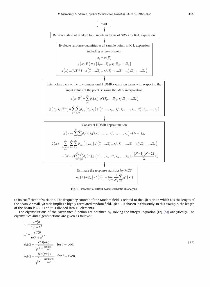
Fig. 1. Flowchart of HDMR-based stochastic FE analysis.


to its coefficient of variation. The frequency content of the random field is related to the L/b ratio in which L is the length ofthe beam. A small L/b ratio implies a highly correlated random field. L/b = 1 is chosen in this study. In this example, the lengthof the beam is L = 1 and it is divided into 10 elements.

The eigensolutions of the covariance function are obtained by solving the integral equation (Eq. (5)) analytically. Theeigenvalues and eigenfunctions are given as follows:

ki ¼2r2

ab

x2i þ b2 ;

k�i ¼2r2

ab

x�2i þ b2 ;

wiðnÞ ¼cosðxinÞffiffiffiffiffiffiffiffiffiffiffiffiffiffiffiffiffiffiffiffiffiffiffiaþ sinð2xinÞ

2xi

q for i ¼ odd;

wiðnÞ ¼sinðx�i nÞffiffiffiffiffiffiffiffiffiffiffiffiffiffiffiffiffiffiffiffiffiffiffia� sinð2x�

inÞ

2x�i

r for i ¼ even:

ð27Þ

(a) (b)

x

x

x1

x2

x

Fig. 2. Sampling scheme for first-order HDMR; (a) for a function having one variable (x); and (b) for a function having two variables (x1 and x2).

x1

x2

x

Fig. 3. Sampling scheme for second-order HDMR for a function having two variables (x1 and x2).

L = 1 m

P = 300 N

Fig. 4. Cantilever beam.


The random field is discretized into ten SRVs, and the 10-term K–L expansion (Eq. (7)) is used to generate sample func-tions of the input random field. The response quantity which is the tip displacement of the beam is represented by HDMRexpansion with five sample points. To evaluate the validity of the results obtained from the proposed method full scale MCSis performed for the same problem. Realizations of the elastic modulus of the beam are numerically simulated using the K–Lexpansion method. For each of the realizations, the deterministic problem is solved and the statistics of the response areobtained. Fig. 4 compares the probability density functions obtained from first- and second-order HDMR with full scaleMCS. Excellent agreements are observed between the proposed approach and 1 � 104 full scale MCS results. The cumulativedistribution function is shown in Fig. 5.

Compared with the first two response moments obtained using direct MCS (m1 = 3.778 � 10�2, m2 = 7.690 � 10�3), pres-ent method using first-order HDMR approximation, underestimates the first two moments by 0.27% (m1 = 3.768 � 10�2) and1.41% (m2 = 7.582 � 10�3), respectively, while second-order HDMR approximation, underestimates the first two moments by0.02% (m1 = 3.777 � 10�2) and 0.47% (m2 = 7.654 � 10�3), respectively. The present method using first- and second-orderHDMR approximation needs 41 and 761 original FE analysis, respectively, while full scale MCS requires 1 � 104 numberof original FE calculation. This shows the accuracy and the efficiency (in terms of FE analysis) of the present method usingfirst-order HDMR approximation, direct MCS.

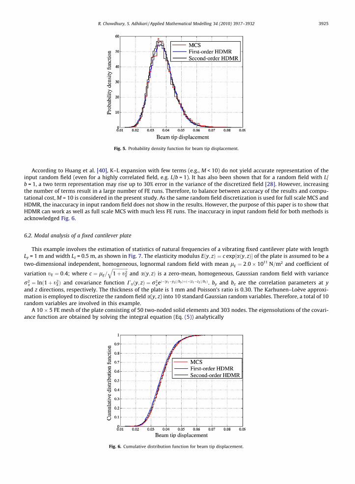
Fig. 5. Probability density function for beam tip displacement.


According to Huang et al. [40], K–L expansion with few terms (e.g., M < 10) do not yield accurate representation of theinput random field (even for a highly correlated field, e.g. L/b = 1). It has also been shown that for a random field with L/b = 1, a two term representation may rise up to 30% error in the variance of the discretized field [28]. However, increasingthe number of terms result in a large number of FE runs. Therefore, to balance between accuracy of the results and compu-tational cost, M = 10 is considered in the present study. As the same random field discretization is used for full scale MCS andHDMR, the inaccuracy in input random field does not show in the results. However, the purpose of this paper is to show thatHDMR can work as well as full scale MCS with much less FE runs. The inaccuracy in input random field for both methods isacknowledged Fig. 6.

6.2. Modal analysis of a fixed cantilever plate

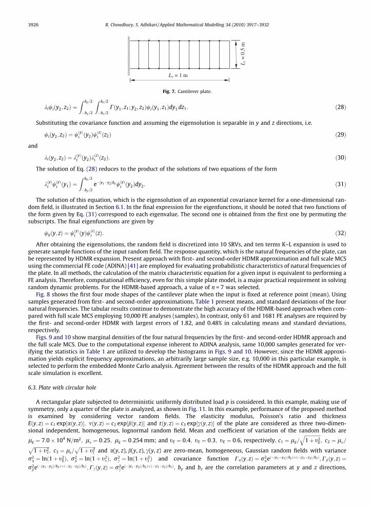
This example involves the estimation of statistics of natural frequencies of a vibrating fixed cantilever plate with lengthLy = 1 m and width Lz = 0.5 m, as shown in Fig. 7. The elasticity modulus Eðy; zÞ ¼ c exp½aðy; zÞ� of the plate is assumed to be atwo-dimensional independent, homogeneous, lognormal random field with mean lE ¼ 2:0� 1011 N=m2 and coefficient of

variation tE ¼ 0:4; where c ¼ lE=ffiffiffiffiffiffiffiffiffiffiffiffiffiffi1þ t2

E

qand aðy; zÞ is a zero-mean, homogeneous, Gaussian random field with variance

r2a ¼ lnð1þ t2

EÞ and covariance function Caðy; zÞ ¼ r2aeð�jy1�y2 j=byÞþð�jz1�z2 j=bzÞ. by and bz are the correlation parameters at y

and z directions, respectively. The thickness of the plate is 1 mm and Poisson’s ratio is 0.30. The Karhunen–Loève approxi-mation is employed to discretize the random field a(y, z) into 10 standard Gaussian random variables. Therefore, a total of 10random variables are involved in this example.

A 10 � 5 FE mesh of the plate consisting of 50 two-noded solid elements and 303 nodes. The eigensolutions of the covari-ance function are obtained by solving the integral equation (Eq. (5)) analytically

Fig. 6. Cumulative distribution function for beam tip displacement.

Lz =

0.5

m

Ly = 1 m

Fig. 7. Cantilever plate.


kiwiðy2; z2Þ ¼Z by=2

�by=2

Z bz=2

�bz=2Cðy1; z1; y2; z2Þwiðy1; z1Þdy1 dz1: ð28Þ

Substituting the covariance function and assuming the eigensolution is separable in y and z directions, i.e.

wiðy2; z2Þ ¼ wðyÞi ðy2ÞwðzÞi ðz2Þ ð29Þ

and

kiðy2; z2Þ ¼ kðyÞi ðy2ÞkðzÞi ðz2Þ: ð30Þ

The solution of Eq. (28) reduces to the product of the solutions of two equations of the form

kðyÞi wðyÞi ðy1Þ ¼Z by=2

�by=2e�jy1�y2 jby wðyÞi ðy2Þdy2: ð31Þ

The solution of this equation, which is the eigensolution of an exponential covariance kernel for a one-dimensional ran-dom field, is illustrated in Section 6.1. In the final expression for the eigenfunctions, it should be noted that two functions ofthe form given by Eq. (31) correspond to each eigenvalue. The second one is obtained from the first one by permuting thesubscripts. The final eigenfunctions are given by

wkðy; zÞ ¼ wðyÞi ðyÞwðzÞi ðzÞ: ð32Þ

After obtaining the eigensolutions, the random field is discretized into 10 SRVs, and ten terms K–L expansion is used togenerate sample functions of the input random field. The response quantity, which is the natural frequencies of the plate, canbe represented by HDMR expansion. Present approach with first- and second-order HDMR approximation and full scale MCSusing the commercial FE code (ADINA) [41] are employed for evaluating probabilistic characteristics of natural frequencies ofthe plate. In all methods, the calculation of the matrix characteristic equation for a given input is equivalent to performing aFE analysis. Therefore, computational efficiency, even for this simple plate model, is a major practical requirement in solvingrandom dynamic problems. For the HDMR-based approach, a value of n = 7 was selected.

Fig. 8 shows the first four mode shapes of the cantilever plate when the input is fixed at reference point (mean). Usingsamples generated from first- and second-order approximations, Table 1 present means, and standard deviations of the fournatural frequencies. The tabular results continue to demonstrate the high accuracy of the HDMR-based approach when com-pared with full scale MCS employing 10,000 FE analyses (samples). In contrast, only 61 and 1681 FE analyses are required bythe first- and second-order HDMR with largest errors of 1.82, and 0.48% in calculating means and standard deviations,respectively.

Figs. 9 and 10 show marginal densities of the four natural frequencies by the first- and second-order HDMR approach andthe full scale MCS. Due to the computational expense inherent to ADINA analysis, same 10,000 samples generated for ver-ifying the statistics in Table 1 are utilized to develop the histograms in Figs. 9 and 10. However, since the HDMR approxi-mation yields explicit frequency approximations, an arbitrarily large sample size, e.g. 10,000 in this particular example, isselected to perform the embedded Monte Carlo analysis. Agreement between the results of the HDMR approach and the fullscale simulation is excellent.

6.3. Plate with circular hole

A rectangular plate subjected to deterministic uniformly distributed load p is considered. In this example, making use ofsymmetry, only a quarter of the plate is analyzed, as shown in Fig. 11. In this example, performance of the proposed methodis examined by considering vector random fields. The elasticity modulus, Poisson’s ratio and thicknessEðy; zÞ ¼ c1 exp½aðy; zÞ�; mðy; zÞ ¼ c2 exp½bðy; zÞ� and tðy; zÞ ¼ c3 exp½cðy; zÞ� of the plate are considered as three two-dimen-sional independent, homogeneous, lognormal random field. Mean and coefficient of variation of the random fields are

lE ¼ 7:0� 104 N=m2; lm ¼ 0:25; lE ¼ 0:254 mm; and tE ¼ 0:4; tE ¼ 0:3; tE ¼ 0:6, respectively. c1 ¼ lE=ffiffiffiffiffiffiffiffiffiffiffiffiffiffi1þ t2

E

q; c2 ¼ lm=ffiffiffiffiffiffiffiffiffiffiffiffiffiffi

1þ t2m

p; c3 ¼ lt=

ffiffiffiffiffiffiffiffiffiffiffiffiffiffi1þ t2

t

pand a(y, z), b(y, z), c(y, z) are zero-mean, homogeneous, Gaussian random fields with variance

r2a ¼ lnð1þ t2

EÞ; r2b ¼ lnð1þ t2

mÞ; r2c ¼ lnð1þ t2

t Þ and covariance function Caðy; zÞ ¼ r2aeð�jy1�y2 j=byÞþð�jz1�z2 j=bzÞ;Cbðy; zÞ ¼

r2beð�jy1�y2 j=byÞþð�jz1�z2 j=bzÞ;Ccðy; zÞ ¼ r2

ceð�jy1�y2 j=byÞþð�jz1�z2 j=bzÞ. by and bz are the correlation parameters at y and z directions,

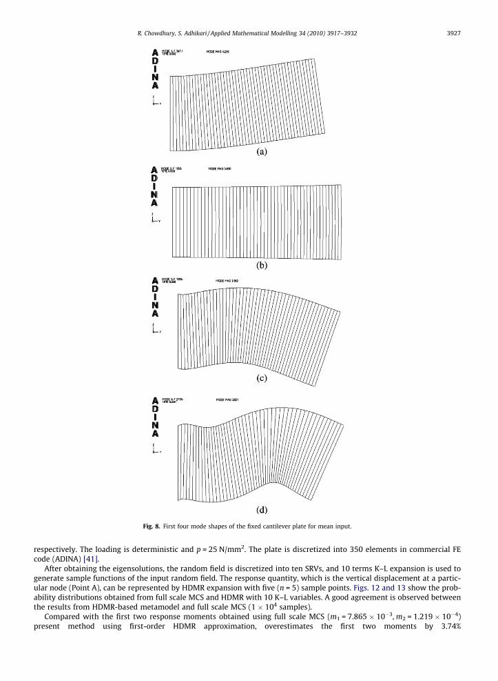
Fig. 8. First four mode shapes of the fixed cantilever plate for mean input.


respectively. The loading is deterministic and p = 25 N/mm2. The plate is discretized into 350 elements in commercial FEcode (ADINA) [41].

After obtaining the eigensolutions, the random field is discretized into ten SRVs, and 10 terms K–L expansion is used togenerate sample functions of the input random field. The response quantity, which is the vertical displacement at a partic-ular node (Point A), can be represented by HDMR expansion with five (n = 5) sample points. Figs. 12 and 13 show the prob-ability distributions obtained from full scale MCS and HDMR with 10 K–L variables. A good agreement is observed betweenthe results from HDMR-based metamodel and full scale MCS (1 � 104 samples).

Compared with the first two response moments obtained using full scale MCS (m1 = 7.865 � 10�3, m2 = 1.219 � 10�4)present method using first-order HDMR approximation, overestimates the first two moments by 3.74%

Table 1Means and standard deviations of first four natural frequencies for the cantilever plate.a

Frequency Mean Standard deviation

First-order HDMR Second-order HDMR Monte Carlo First-order HDMR Second-order HDMR Monte Carlo

1 338.15 336.14 336.42 38.98 38.75 38.81(�0.51) (0.08) (�0.44) (0.15)

2 1200.17 1216.48 1222.42 134.56 134.02 133.92(1.82) (0.49) (�0.48) (�0.07)

3 1274.76 1266.88 1267.01 133.39 132.88 132.81(�0.61) (0.01) (�0.44) (�0.05)

4 2690.20 2668.0 2664.58 250.98 250.42 250.44(�0.96) (�0.13) (�0.22) (0.01)

a Parenthetical values represent percentage of relative errors when compared with the full scale MCS.

Fig. 9. Probability densities of first four natural frequencies.


(m1 = 8.159 � 10�3) and 39.34% (m2 = 7.394 � 10�5), respectively, while second-order HDMR approximation, overestimatesthe first two moments by 0.42% (m1 = 7.898 � 10�3) and 4.68% (m2 = 1.274 � 10�4), respectively. However, the present meth-od using first- and second-order HDMR approximation needs 41 and 761 original FE analysis, respectively, while full scaleMCS requires 1 � 104 number of original FE calculation. This shows the accuracy and the efficiency (in terms of FE analysis)of the present method using first-order HDMR approximation, direct MCS.

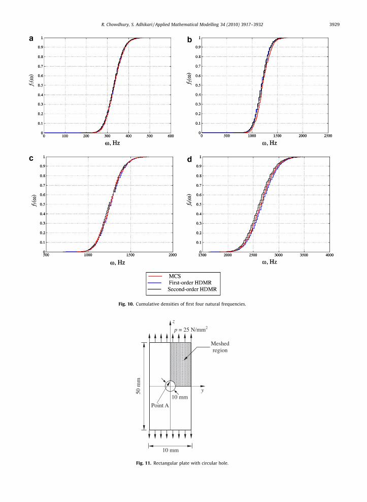
Fig. 10. Cumulative densities of first four natural frequencies.

10 mm

50 m

m

y

z

10 mm

Meshedregion

p = 25 N/mm2

Point A

Fig. 11. Rectangular plate with circular hole.


Fig. 12. Probability density function for the vertical displacement at point A of the plate.

Fig. 13. Cumulative distribution function for the vertical displacement at point A of the plate.


7. Summary and conclusions

This paper presents extended HDMR approach for problems in which physical properties exhibit spatial random varia-tion. The method appears to be efficient, requiring only conditional responses at selected sample points to accurately com-pute solution statistics. In comparison, full scale MCS may require thousands of realizations or more for converged statistics.Thus the proposed method substantially reduces the computational effort while maintaining the desired accuracy. K–Lexpansion is required for discretizing the input random field with many terms, which in turn can increase the dimensionalityof the problem and thus the computational effort of the SFEM. The curse of dimensionality, which is a problem in other cur-rently available methods, does not arise in the proposed approach. This is because it discretizes the whole problem into anumber of subproblems.

Also, the proposed method is independent of the details of structural analysis (in the context of commercial software) as ittreats the FE model as a black box. If higher loads introduce nonlinearity in the model response, then the appropriate non-linear analysis should be used, and the underlying HDMR-based metamodel would automatically be different. Thus the pro-posed method is applicable to the analysis of linear as well as nonlinear structures, provided the right FE software is used.Good agreements are observed comparing the numerical results between extended HDMR and full scale MCS. However, fol-lowing observations can be made easily from this article:

Computational effort: HDMR-based approach requires conditional responses at selected sample points and the samplepoints are chosen along each of the variable axis. It is found in authors’ previous work that n = 5 or 7 works well for mostthe problem. Due to this fact, results for n = 5 or 7 are used in this paper to construct HDMR-based metamodels.

Handling spatial variability: Unlike local expansion based methods such as perturbation and Neumann expansion meth-ods HDMR can accurately handle random fields with moderate to large coefficients of variations.


8. Discussion and outlook

In this paper, HDMR-based approximation methods are developed in a comprehensive way for structural mechanicsproblem with random fields. The presented method couples the commercial FE codes and full scale simulation throughapproximate models. Formally, Eqs. (17) and (18) can be interpreted as higher order response surface for the response field,defined by means of input random field(s). In contrast with usual response surface methods (e.g. polynomial chaos), HDMRapproximation allows to define it at any order in a consistent framework. The following notable advantages of the proposedmethod may be recognized:

HDMR is a finite sum that contains 2N � 1 number of summands and N random variables. In contrast, the polynomialchaos expansion is an infinite series and contains an infinite number of random variables. Therefore, if the componentfunctions in Eq. (9) are convergent, then HDMR approximation provides a convergent solution. The terms in the polynomial chaos expansion are organized with respect to the order of polynomials. On the other hand,

HDMR is structured with respect to the degree of cooperativity between a finite number of random variables. If a responseis highly nonlinear but contains rapidly diminishing cooperative effects of multiple random variables, HDMR approxima-tion is effective. This is due to the fact that, lower-order HDMR approximation can inherently incorporate nonlineareffects in system characteristics. In contrast, many terms are required to be included in the polynomial chaos expansionto capture high nonlinearity. The proposed method is independent of the structural analysis (in the context of commercial software) as it treats the FE

model as a black box. If the material/geometrical nonlinearity is introduced in the model response, then the appropriatenonlinear analysis should be selected, and the underlying HDMR-based metamodel would automatically be different. The amount of computation required for a given problem in SSFEM grows factorially, whereas, in the proposed approach

it varies either polynomially.

Note that in all applications found in this paper, only the K–L expansion is used to discretize the input random field(s).The use of other schemes would however be possible and in some case more practical than K–L (for instance when othercorrelation structures than that with exponential decay are dealt with). Future work will address these issues.

Acknowledgements

RC would like to acknowledge the support of Royal Society through the award of Newton International Fellowship. SAwould like to acknowledge the support of UK Engineering and Physical Sciences Research Council (EPSRC) through the awardof an Advanced Research Fellowship and The Leverhulme Trust for the award of the Philip Leverhulme Prize.

References

[1] M. Grigoriu, Reduced order models for random functions. Application to stochastic problems, Appl. Math. Model. 33 (1) (2009) 161–175.[2] Y. Kerboua, A.A. Lakis, M. Thomas, L. Marcouiller, Vibration analysis of rectangular plates coupled with fluid, Appl. Math. Model. 32 (12) (2008) 2570–

2586.[3] Z. Qiu, J. Hu, Two non-probabilistic set-theoretical models to predict the transient vibrations of cross-ply plates with uncertainty, Appl. Math. Model.

32 (12) (2008) 2872–2887.[4] S. Murugan, D. Harursampath, R. Ganguli, Material uncertainty propagation in helicopter nonlinear aeroelastic response and vibration analysis, AIAA J.

46 (9) (2008) 2332–2344.[5] M. Chandrashekhar, R. Ganguli, Uncertainty handling in structural damage detection using fuzzy logic and probabilistic simulation, Mech. Syst. Signal

Process. 23 (2) (2009) 384–404.[6] S. Murugan, R. Ganguli, D. Harursampath, Aeroelastic analysis of composite helicopter rotor with random material properties, AIAA J. Aircraft 45 (1)

(2008) 306–322.[7] R. Ghanem, P.D. Spanos, Stochastic Finite Elements: A Spectral Approach, Dover Publications Inc., New York, 2002.[8] W.K. Liu, T. Belytschko, A. Mani, Random field finite elements, Int. J. Numer. Methods Eng. 23 (10) (1986) 1831–1845.[9] F. Yamazaki, M. Shinozuka, Neumann expansion for stochastic finite element analysis, J. Eng. Mech. ASCE 114 (8) (1988) 1335–1354.

[10] S. Adhikari, Reliability analysis using parabolic failure surface approximation, J. Eng. Mech. ASCE 130 (12) (2004) 1407–1427.[11] S. Adhikari, Asymptotic distribution method for structural reliability analysis in high dimensions, Proc. Roy. Soc. London Ser. A 461 (2062) (2005)

3141–3158.[12] O. Ditlevsen, H.O. Madsen, Structural Reliability Methods, Wiley, Chichester, 1996.[13] RY. Rubinstein, Simulation and the Monte Carlo Method, Wiley, New York, 1981.[14] D. Ghiocel, R. Ghanem, Stochastic finite element analysis of seismic soil–structure interaction, J. Eng. Mech. ASCE 128 (1) (2002) 66–77.[15] R. Chowdhury, B.N. Rao, A.M. Prasad, High dimensional model representation for structural reliability analysis, Commun. Numer. Methods Eng. 25 (4)

(2009) 301–337.[16] R. Chowdhury, B.N. Rao, Assessment of high dimensional model representation techniques for reliability analysis, Probab. Eng. Mech. 24 (1) (2009)

100–115.[17] R. Chowdhury, B.N. Rao, Hybrid high dimensional model representation for reliability analysis, Comput. Methods Appl. Mech. Eng. 198 (5–8) (2009)

735–765.[18] B.N. Rao, R. Chowdhury, Enhanced high dimensional model representation for reliability analysis, Int. J. Numer. Methods Eng. 77 (5) (2009) 719–750.[19] H.L. Van Trees, Detection Estimation and Modulation Theory: Part 1, John Wiley & Sons, New York, 1968.[20] H. Rabitz, O.F. Alis, J. Shorter, K. Shim, Efficient input–output model representations, Comput. Phys. Commun. 117 (1–2) (1999) 11–20.[21] H. Rabitz, O.F. Alis, General foundations of high dimensional model representations, J. Math. Chem. 25 (2–3) (1999) 197–233.[22] S. Huang, S. Mahadevan, R. Rebba, Collocation-based stochastic finite element analysis for random field problems, Probab. Eng. Mech. 22 (2) (2007)

194–205.


[23] B. Sudret, A. Der Kiureghian, Stochastic Finite Element Methods and Reliability: A State-of-the-Art Report, Tech. Rep. UCB/SEMM-2000/08, Universityof California, Berkley, USA, 2000.

[24] A. Der Kiureghian, J.B. Ke, The stochastic finite element method in structural reliability, Probab. Eng. Mech. 3 (2) (1988) 83–91.[25] W.K. Liu, T. Belytschko, A. Mani, Probabilistic finite elements for nonlinear structural dynamics, Comput. Methods Appl. Mech. Eng. 56 (1) (1986) 61–

86.[26] G. Matthies, C. Brenner, C. Bucher, C. Guedes Soares, Uncertainties in probabilistic numerical analysis of structures and solids � stochastic finite

elements, Struct. Saf. 19 (3) (1997) 283–336.[27] C.C. Li, A. Der Kiureghian, Optimal discretization of random fields, J. Eng. Mech. ASCE 119 (6) (1993) 1136–1154.[28] E. Vanmarcke, Random Fields: Analysis and Synthesis, The MIT Press, Cambridge, Massachussets, 1983.[29] E.H. Vanmarcke, M. Grigoriu, Stochastic finite element analysis of simple beams. J. Eng. Mech., ASCE 109(5) (1083) 1203–1214.[30] G. Deodatis, The weighted integral method, I: Stochastic stiffness matrix, J. Eng. Mech. ASCE 117 (8) (1991) 1851–1864.[31] G. Deodatis, M. Shinozuka, The weighted integral method, II : Response variability and reliability, J. Eng. Mech. ASCE 117 (8) (1991) 1865–1877.[32] T. Takada, Weighted integral method in multidimensional stochastic finite element analysis, Probab. Eng. Mech. 5 (4) (1990) 158–166.[33] T. Takada, Weighted integral method in stochastic finite element analysis, Probab. Eng. Mech. 5 (3) (1990) 146–156.[34] J. Zhang, B. Ellingwood, Orthogonal series expansion of random fields in reliability analysis, J. Eng. Mech. ASCE 120 (12) (1994) 2660–2677.[35] P. Devijver, J. Kittler, Pattern Recognition: A Statistical Approach, Prentice-Hall, London, UK, 1982.[36] S. Adhikari, Response variability of linear stochastic systems: a general solution using random matrix theory, in: 49th AIAA/ASME/ASCE/AHS/ASC

Structures, Structural Dynamics and Materials Conference, Schaumburg, IL, USA, April 2008.[37] I.M. Sobol, Theorems and examples on high dimensional model representations, Reliabil. Eng. Syst. Safety 79 (2) (2003) 187–193.[38] G. Li, C. Rosenthal, H. Rabitz, High dimensional model representations, J. Phys. Chem. A 105 (2001) 7765–7777.[39] P. Lancaster, K. Salkauskas, Curve and Surface Fitting: An Introduction, Academic Press, London, 1986.[40] S.P. Huang, S.T. Quek, K.K. Phoon, Convergence study of the truncated Karhunen–Loeve expansion for simulation of stochastic processes, Int. J. Numer.

Methods Eng. 52 (2001) 1029–1043.[41] ADINA R&D, Inc., ADINA Theory and Modeling Guide, Report ARD 05 6, 2005.

applied mathematical modelling - swansea...

Documents