applied geophysics – oct 6 · applied geophysics – oct 6 goals for today review time-intercept...

Applied Geophysics –

Oct 6

Goals for today

Review time-intercept method

Sources/Receivers

Low velocity zones (applet for Snell’s law)

Multiple Layers

Other interpretation methods (Plus-Minus)

Preparation for TBL

A B

A B

Seismic surveyoffset

…

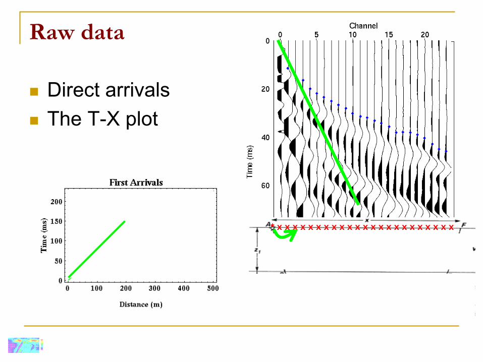
Raw data

Direct arrivals

The T-X plot

* x x x x x x x x x x x x x x x x x x x x x x x

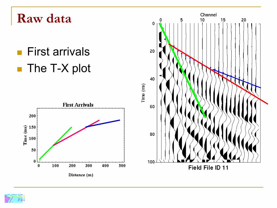
Raw data

First refractions

The T-X plot


Raw data

Second refractions

The T-X plot


Raw data

First arrivals

The T-X plot

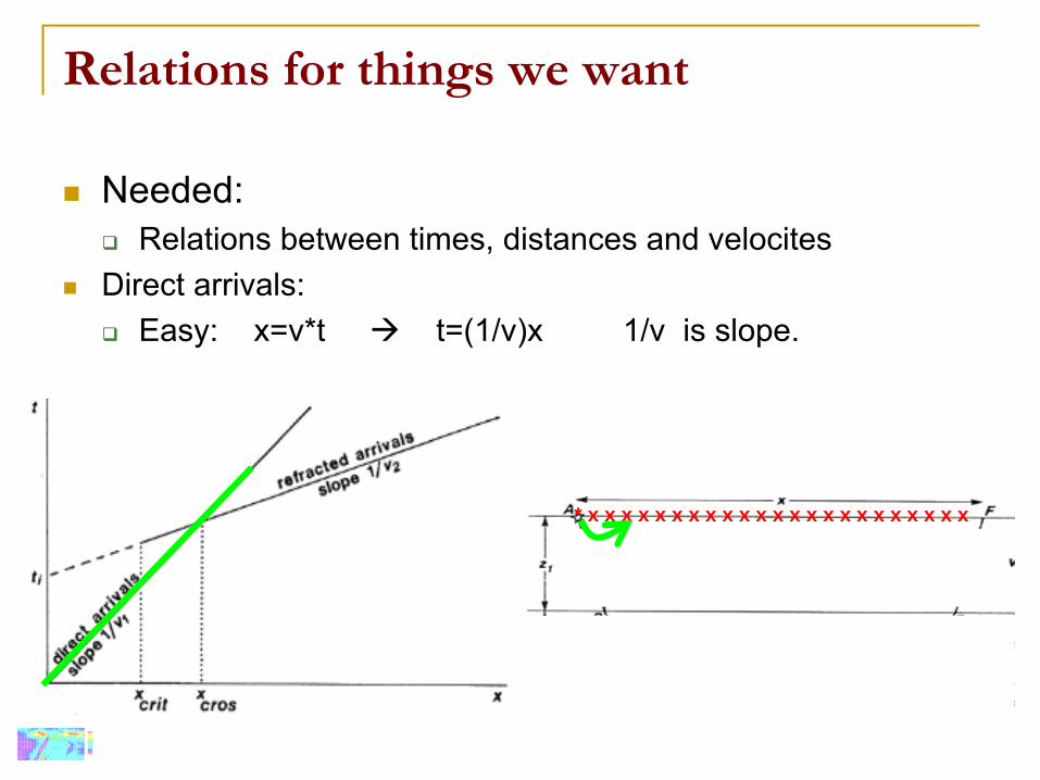
Relations for things we want

Needed:

Relations between times, distances and velocites

Direct arrivals:

Easy: x=v*t

t=(1/v)x 1/v is slope.


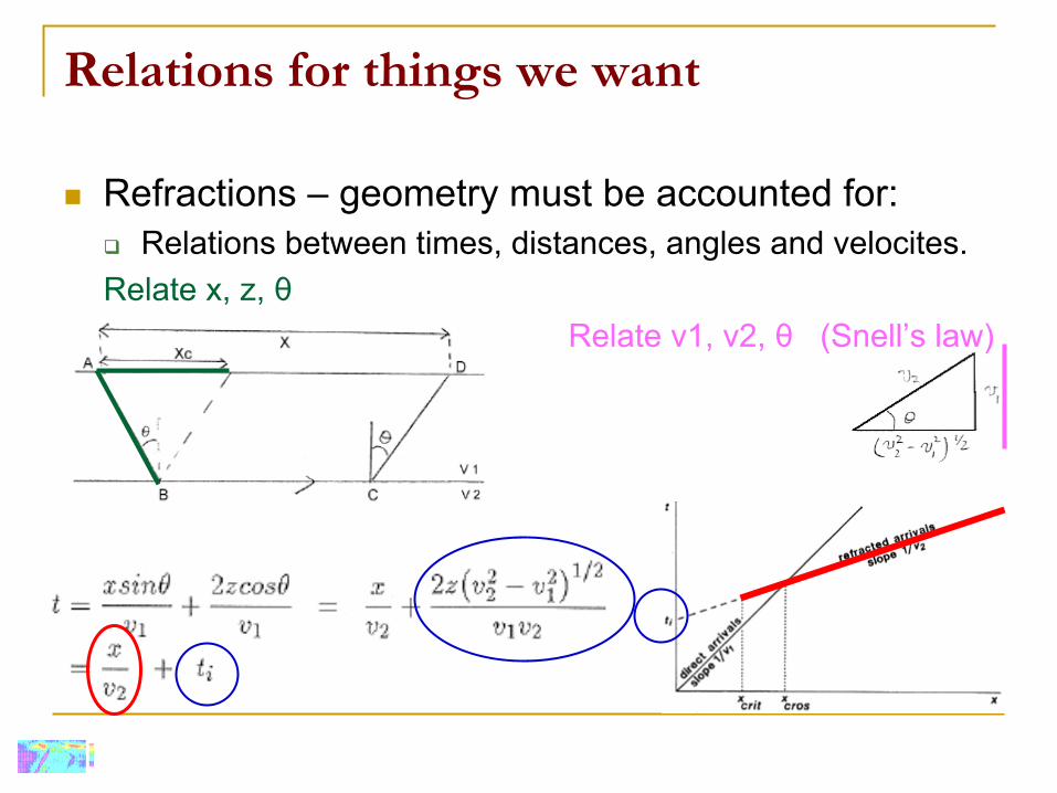
Relations for things we want

Refractions –

geometry must be accounted for:

Relations between times, distances, angles and velocites.Relate x, z, θ

Relate v1, v2, θ

(Snell’s law)

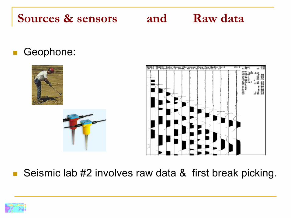
Sources & sensors and Raw data

Geophone:

Seismic lab #2 involves raw data & first break picking.

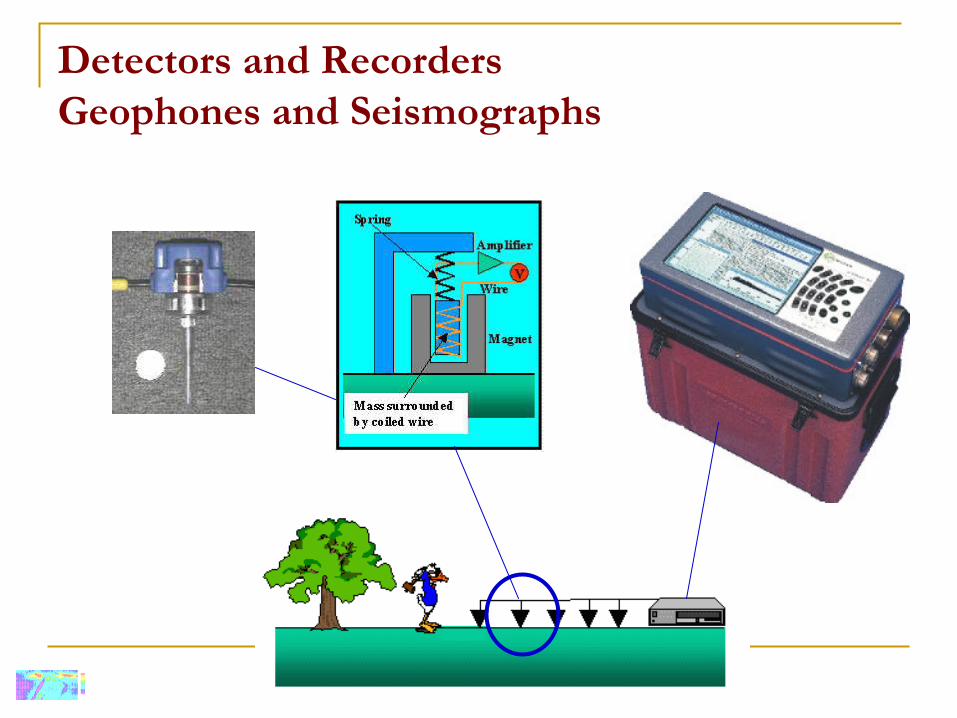
Detectors and Recorders Geophones and Seismographs

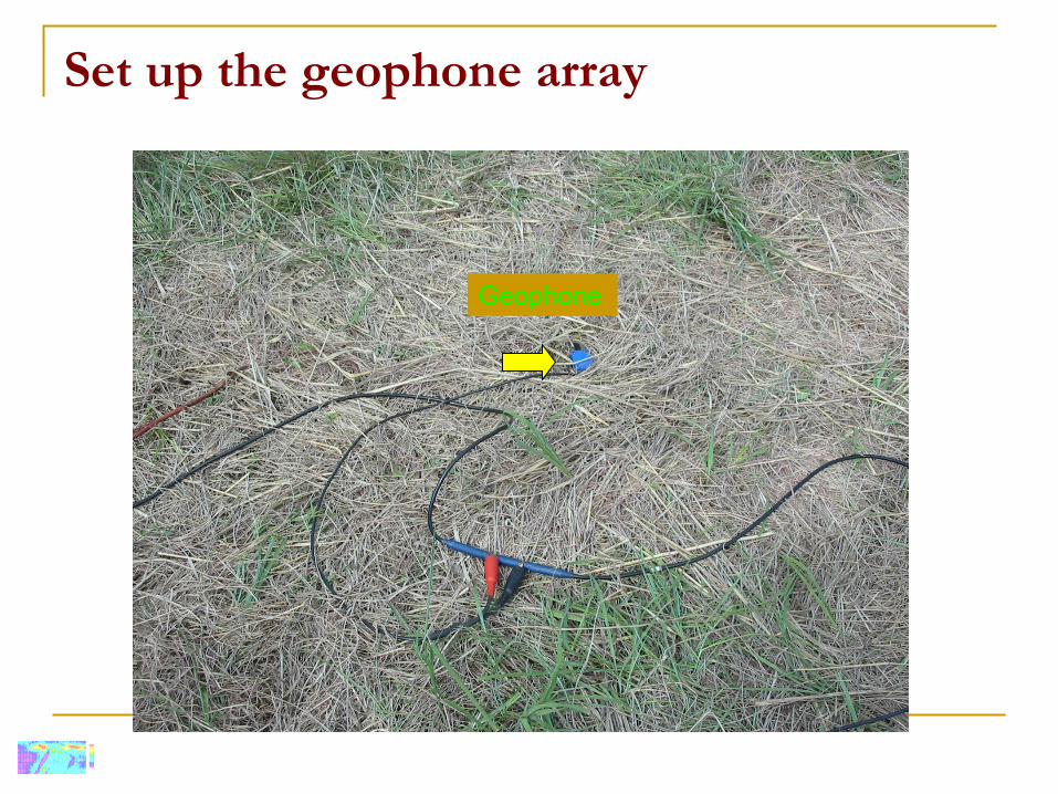
Set up the geophone array

Geophone

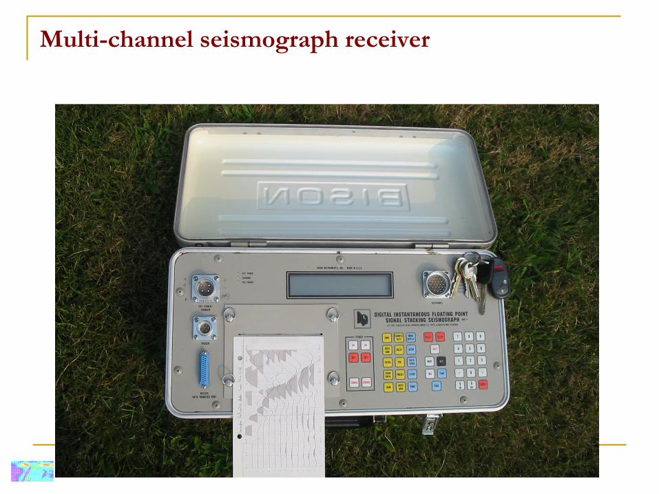
Multi-channel seismograph receiver

Borehole explosion

http://en.wikipedia.org/wiki/Image:Explosions.jpg

Thumper truck

From Lithoprobe

website

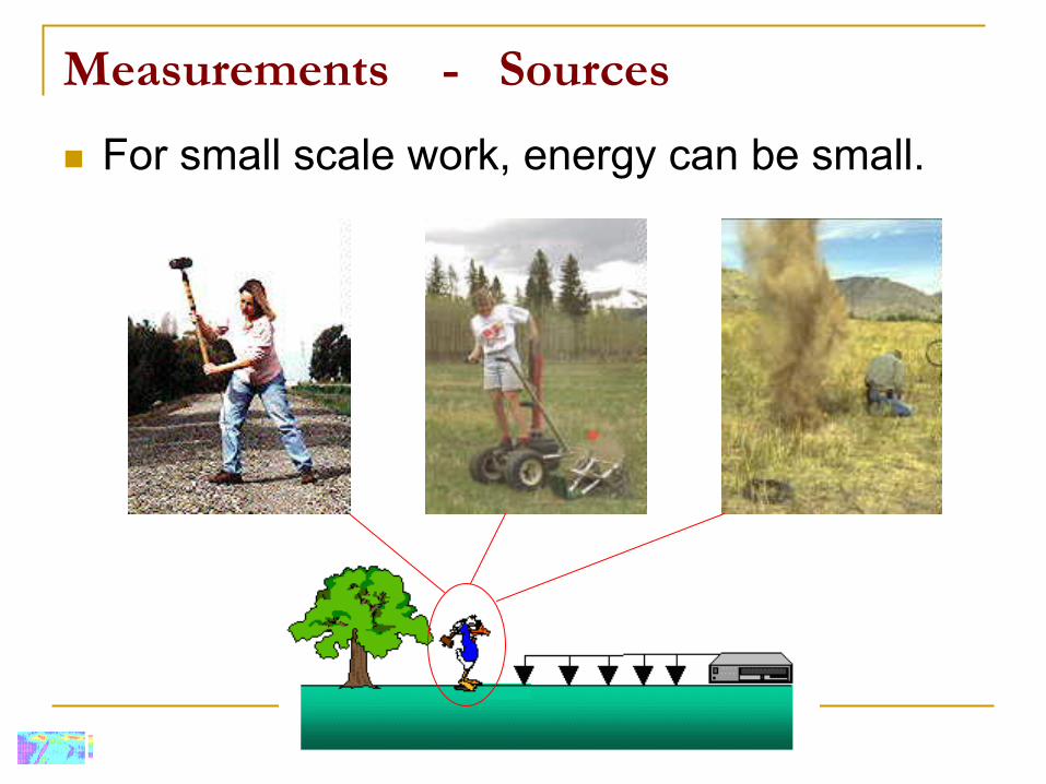
Measurements - Sources

For small scale work, energy can be small.

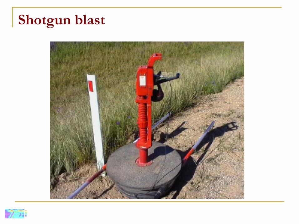
Shotgun blast

Sledge hammer

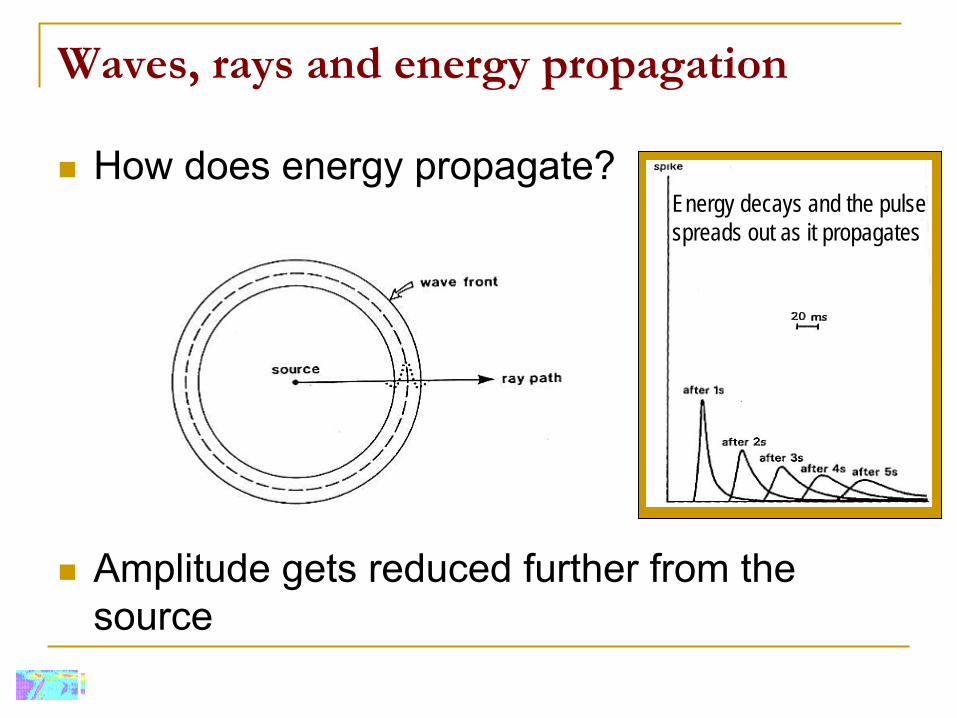
Waves, rays and energy propagation

How does energy propagate?

Amplitude gets reduced further from the source

Energy decays and the pulse spreads out as it propagates

EOSC 350 ‘06 Slide 22

Refraction Seismic

Low Velocity Zones

Refraction for 3 layers.

Dipping Layers

More complicated interfaces and approaches.

Plus-Minus method

Generalized Reciprocal Method

Ray Tracing

Low Velocity Zone

Snell’s law for decreasing velocity

http://staff.washington.edu/aganse/raydemo/RayDemo2.med.html

Ray tracing for non-layered velocity models (Illustration of Snell’s law)

http://staff.washington.edu/aganse/raydemo/RayDemo2.med.html

Low Velocity Zones

V2 < v1

No refracted arrival from the top of the second layer

Hidden Layer

Layers that are too thin may not be seen

Arrival from layer 3beats that from layer 2

V3>v2>v1

Refraction 3-layers: Snell’s law rules

Second refractions

The T-X plot


Intercept time method (ITM)

What’s ultimately wanted from a seismic refraction survey?

Velocities

From slopes

Depth

From intercept time

ti


Dipping layers: interpretation requires two shots

Resulting T-X plot

Recall: dipping layers

ud

ud

VV

VV

VV

VV

2

11

2

11

2

11

2

11

sinsin21

sinsin21

XShot point

XShot point

Reciprocal time

Depth estimates

“Slant”

depths can be obtained through the intercept times

True depths can be estimated using dip-angle (see GPG 3.e.6)

Irregular Layers

What happens when boundary can no longer be approximated with a plane?

Plus-Minus Methods

GRM (Generalized Reciprocal Methods)

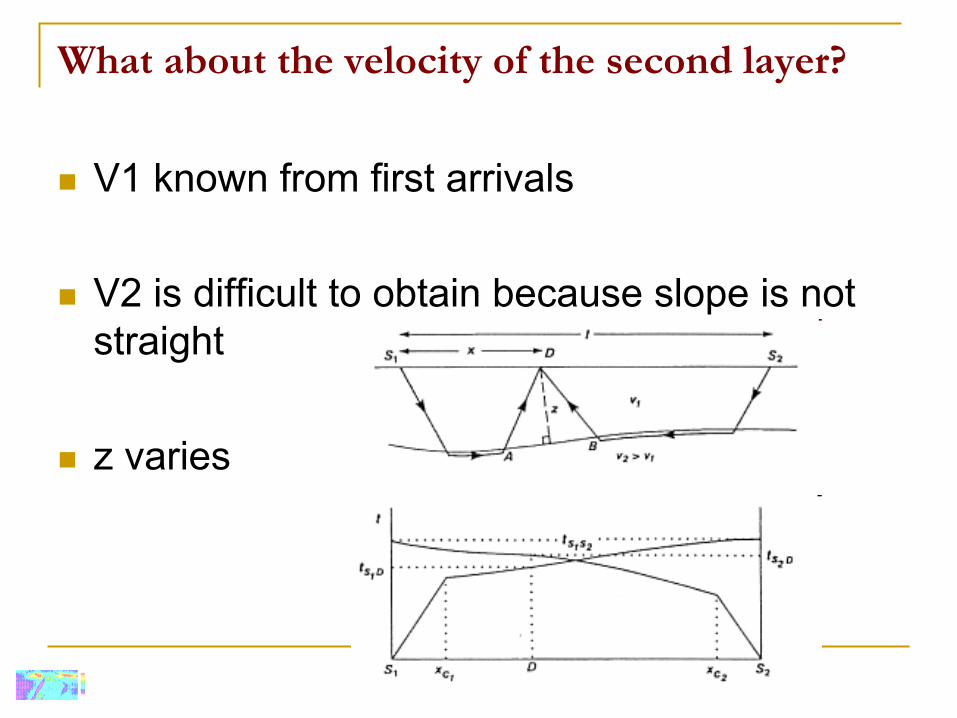
What about the velocity of the second layer?

V1 known from first arrivals

V2 is difficult to obtain because slope is not straight

z varies


The Plus-Minus method Notes section 8.

We want Z = depth under geophones

We could do

But we don’t know TAD

cos1VTZ AD


Delay timeWe want depth, z, under D.

Relation is 1st

to the right

aSD

is the “delay time”, defined as TAB

– TBC

Derivation discussed in notes section 8.


Plus Minus method summaryWe want depth, z, under D.

Relation is 1st

to the right

aSD ’s

value comes from 2nd

relation, called the “Plus term”.

V2 comes from slope of the 3rd

equation, called the “Minus term”.

(Note that the slope is 2/V2

).


Generalized Reciprocal Method -

GRM

ITM with fwd/rvrs

shots, and PlusMinus are “reciprocal methods”.

Goal of GRM is to estimate velocities & depths without requiring interface segments that are flat.

Velocity and depth BOTH estimated under EACH geophone that has seen refractions.

Therefore lateral

velocity variations in one layer can be seen.

But …

“smooth”

velocity changes (materials grading one into the other) can still not be seen.

GRM interpretation

Can be performed along a line (see GPG e.10)

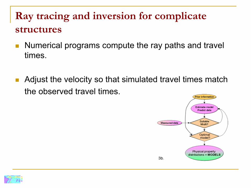
Ray tracing and inversion for complicate structures

Numerical programs compute the ray paths and travel times.

Adjust the velocity so that simulated travel times match the observed travel times.


Ray tracing techniques

Created data must look like measured data, within error bars. Therefore error specifications are an important part of the data

set.

Also “turning rays”

can be accommodated.

Interfaces are not necessary because steadily increasing velocity means ray paths curve.

This effect is crucial

in crustal studies

using earthquake

signals.

Of course, head waves

are also handled

properly.


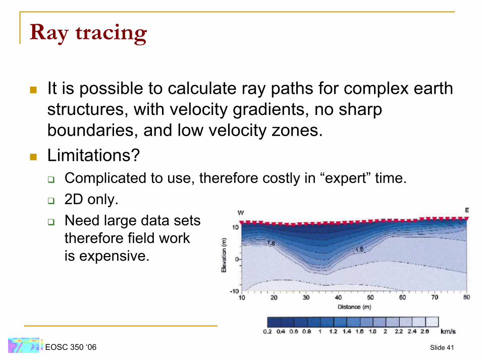
Ray tracing

It is possible to calculate ray paths for complex earth structures, with velocity gradients, no sharp boundaries, and low velocity zones.

Limitations?

Complicated to use, therefore costly in “expert”

time.

2D only.

Need large data sets therefore field work

is expensive.

Reading for Team Exercise

Near-surface SH-wave surveys in unconsolidated, alluvial sediments (on website)

This is a case history for a landfill in Norman, Oklahoma

Pay attention to:

7-Step Process

Understand data plots

Typical data plots

Upcoming

TBL: Friday, October 8 (Near Surface SH)

Monday October 11: Holiday (Thanksgiving)

Wednesday Oct 13: Seismology

Friday October 15: Finish Seismology and other review

Monday: October 17: Quiz (with TBL)

Wednesday Oct. 20: Midterm (physical properties,7 Step procedure, magnetics, seismic refraction; lab material, team exercises)

Global Earthquake

Global Earthquake:

http://www.iris.edu/hq/programs/education_and_outreach/visualizations

US Network for global seismic monitoring (see tutorial)

http://www.iris.edu/hq/programs/education_and_outreach/visualizations

applied geophysics – oct 6 · applied geophysics – oct 6 goals for today review time-intercept...

Documents