applied automata theory - home | ernet
TRANSCRIPT
AppliedAutomataTheory
Prof. Dr. Wolfgang ThomasRWTH Aachen
Course Notes compiled byThierry Cachat
Kostas PapadimitropoulosMarkus Schlutter
Stefan Wohrle
November 2, 2005

2

i
Note
These notes are based on the courses “Applied Automata Theory” and“Angewandte Automatentheorie” given by Prof. W. Thomas at RWTHAachen University in 2002 and 2003.
In 2005 they have been revised and corrected but still they may containmistakes of any kind. Please report any bugs you find, comments, andproposals on what could be improved [email protected]

ii

Contents
0 Introduction 1
0.1 Notation . . . . . . . . . . . . . . . . . . . . . . . . . . . . . . 6
0.2 Nondeterministic Finite Automata . . . . . . . . . . . . . . . 6
0.3 Deterministic Finite Automata . . . . . . . . . . . . . . . . . 7
1 Automata and Logical Specifications 9
1.1 MSO-Logic over words . . . . . . . . . . . . . . . . . . . . . . 9
1.2 The Equivalence Theorem . . . . . . . . . . . . . . . . . . . . 16
1.3 Consequences and Applications in Model Checking . . . . . . 28
1.4 First-Order Definability . . . . . . . . . . . . . . . . . . . . . 31
1.4.1 Star-free Expressions . . . . . . . . . . . . . . . . . . . 31
1.4.2 Temporal Logic LTL . . . . . . . . . . . . . . . . . . . 32
1.5 Between FO- and MSO-definability . . . . . . . . . . . . . . . 35
1.6 Exercises . . . . . . . . . . . . . . . . . . . . . . . . . . . . . 39
2 Congruences and Minimization 43
2.1 Homomorphisms, Quotients and Abstraction . . . . . . . . . 43
2.2 Minimization and Equivalence of DFAs . . . . . . . . . . . . . 48
2.3 Equivalence and Reduction of NFAs . . . . . . . . . . . . . . 57
2.4 The Syntactic Monoid . . . . . . . . . . . . . . . . . . . . . . 67
2.5 Exercises . . . . . . . . . . . . . . . . . . . . . . . . . . . . . 74
3 Tree Automata 77
3.1 Trees and Tree Languages . . . . . . . . . . . . . . . . . . . . 78
3.2 Tree Automata . . . . . . . . . . . . . . . . . . . . . . . . . . 82
3.2.1 Deterministic Tree Automata . . . . . . . . . . . . . . 82
3.2.2 Nondeterministic Tree Automata . . . . . . . . . . . . 88
3.2.3 Emptiness, Congruences and Minimization . . . . . . 91
3.3 Logic-Oriented Formalisms over Trees . . . . . . . . . . . . . 94
3.3.1 Regular Expressions . . . . . . . . . . . . . . . . . . . 94
3.3.2 MSO-Logic . . . . . . . . . . . . . . . . . . . . . . . . 99
3.4 XML-Documents and Tree Automata . . . . . . . . . . . . . 102
3.5 Automata over Two-Dimensional Words (Pictures) . . . . . . 109
iii

iv CONTENTS
3.6 Exercises . . . . . . . . . . . . . . . . . . . . . . . . . . . . . 120
4 Pushdown and Counter Systems 1234.1 Pushdown and Counter Automata . . . . . . . . . . . . . . . 1234.2 The Reachability Problem for Pushdown Systems . . . . . . . 1304.3 Recursive Hierarchical Automata . . . . . . . . . . . . . . . . 1364.4 Undecidability Results . . . . . . . . . . . . . . . . . . . . . . 1404.5 Retrospection: The Symbolic Method . . . . . . . . . . . . . 1454.6 Exercises . . . . . . . . . . . . . . . . . . . . . . . . . . . . . 147
5 Communicating Systems 1495.1 Synchronized Products . . . . . . . . . . . . . . . . . . . . . . 1495.2 Communication via FIFO Channels . . . . . . . . . . . . . . 1525.3 Message sequence charts . . . . . . . . . . . . . . . . . . . . . 1565.4 Exercises . . . . . . . . . . . . . . . . . . . . . . . . . . . . . 161
6 Petri Nets 1656.1 Basic Definitions . . . . . . . . . . . . . . . . . . . . . . . . . 1656.2 Petri Nets as Language Acceptors . . . . . . . . . . . . . . . . 1696.3 Matrix Representation of Petri Nets . . . . . . . . . . . . . . 1726.4 Decision Problems for Petri Nets . . . . . . . . . . . . . . . . 1756.5 Exercises . . . . . . . . . . . . . . . . . . . . . . . . . . . . . 180
Index 181
Chapter 0
Introduction
Automata are systems consisting of states, some of them designated as initialor final, and (usually) labeled transitions. In classical automata theoryrecognizable languages or sets of state sequences have been investigated.Non-classical theory deals with several aspects, e.g. infinite sequences andnon terminating behavior, with bisimulation, or with different kinds of inputobjects, e.g. trees as input structures.
Automata (more generally: transition systems) are the main modelingtools in Computer Science. Whenever we want to design a program, aprotocol or an information system, or even just describe what it is intendedto do, its characteristics, and its behavior, we use these special kinds ofdiagrams. Consequently, there is a variety of applications of automata inComputer Science, for example:
• as sequential algorithms (pattern matching, see Figure 1)
They implement exactly those tasks that we normally connect to au-tomata, namely they accept letters as an input, and on terminationthey reach a state, which describes whether or not the text that hasbeen read possesses a certain property.
• as models of the execution structure of algorithms (flow diagrams, seeFigure 2.)
Before actually implementing an algorithm in some programming lan-guage, one usually describes it by using some 2-dimensional model,that represents the steps that a run of this algorithm may take andthe phases that it may go through.
• as a formalism to system description (see Figure 3)
• as a formalism to system specification (see Figure 4)Before developing a system, we want to express its potential capabili-ties.
1

2 CHAPTER 0. INTRODUCTION
q01
0
q11
0q2
0
1
q31
0
q4
0,1
Figure 1: Deterministic automaton searching for 1101
In this course we are almost always concerned with finite automata,which is the area of automata theory where most questions are decidable.As we know, even Turing Machines can be seen as automata, but in thiscase, all main questions are undecidable. On the contrary, in the area offinite automata, practically all interesting questions that one may ask canbe answered by an algorithm; and this is what makes them so special anduseful in Computer Science.
Considered as mathematical objects, automata are simply labeled, di-rected graphs. However, this view on automata is not very interesting, sinceit can only be used to answer rather elementary questions like connectivityor reachability. What makes automata theory more complicated, is the factthat these special kinds of graphs have a certain behavior, they express aspecial meaning. This leads us to the semantics of finite automata. Sometypical kinds of semantics are:
• the language being recognized (consisting of finite or infinite words)
• the word function being computed (automata with output)
• a (bi-)simulation class
• a partial order of actions (in Petri Nets)
• a set of expressions (in tree automata)
By considering these semantics, we can for example define an equivalencebetween two completely different automata in case they recognize exactly thesame language. Moreover one can ask, which one of these two automata isthe “best” in terms of space complexity (e.g. number of states) and whetherthere exists a better automaton. Furthermore, we can ask whether there isa way even to compute the best possible automaton that can recognize thislanguage. Some other questions and problems that arise are listed below.
• Compare automata with respect to their expressive power in defin-ing languages, connect this with alternative formalisms like regularexpressions or logic.

3
Figure 2: Flow diagram

4 CHAPTER 0. INTRODUCTION
Figure 3: Transition diagram

5
Figure 4: SDL-diagram
• Describe and evaluate algorithms for transformation and compositionof automata and evaluate their complexity.
• Is it possible to find the simplest structure or expression to recognizea given language? In the case of automata, simplicity is measured onthe number of states (minimization). In the case of logic formulas itmay be measured e.g. on its length.
• Which questions about automata are decidable and, for those that are,what complexity do the corresponding algorithms have (e.g. concern-ing equivalence)?
Consequently, automata theory has to intersect with other related areasof Computer Science like:
• computability and complexity theory
• logic
• circuit theory
• algorithmic graph theory

6 CHAPTER 0. INTRODUCTION
The course and therefore these course notes are structured as follows:Chapter 1 deals with the connection of automata and logic and with theparadigm of model checking. In Chapter 2 equivalence issues including mini-mization and bisimulation are discussed. Chapter 3 focuses on tree automataand their applications. In Chapter 4 pushdown systems as a first model withan infinite set of configurations are investigated. The next two chapters dealwith automata models which allow communication and concurrency betweendifferent processes, namely communicating finite state machines in Chapter5, including the graphical formalism of message sequence charts, and Petrinets in Chapter 6.
0.1 Notation
An alphabet is a finite set. Its elements are called symbols. We usually denotean alphabet by Σ, and its elements by a, b, c, . . . . A word over an alphabetΣ is a finite sequence of letters a1a2 . . . an with ai ∈ Σ for 1 ≤ i ≤ n. n iscalled the length of a1a2 . . . an. Words are usually named u, v, w, u1, u2, . . . .By ε we denote the word of length 0, i.e. the empty word. Σ∗ (Σ+) is the setof all (nonempty) words over Σ. The concatenation of words u = a1 . . . an
and v = b1 . . . bm is the word uv := a1 . . . anb1 . . . bm. Finally, we use capitalcalligraphic letters A,B, . . . to name automata.
A set L ⊆ Σ∗ is called a language over Σ. Let L, L1, L2 ⊆ Σ∗ be lan-guages. We define the concatenation of L1 and L2 to be the set L1 · L2 :={uv | u ∈ L1 and v ∈ L2}, also denoted by L1L2. We define L0 to be thelanguage {ε}, and Li := LLi−1. The Kleene closure of L is the languageL∗ :=
⋃
i≥0 Li, and the positive Kleene closure L+ is the Kleene closure of
L without adding the empty word, i.e. L+ :=⋃
i≥1 Li.Regular expressions over an alphabet Σ are recursively defined: ∅, ε, and
a for a ∈ Σ are regular expressions denoting the languages ∅, {ε}, and {a}respectively. Let r, s be regular expressions denoting the languages R andS respectively. Then also (r + s), (r · s), and (r∗) are regular expressionsdenoting the languages R ∪ S, RS, and R∗, respectively. We usually omitthe parentheses assuming that ∗ has higher precedence than · and +, andthat · has higher precedence than +.We also denote the regular expression(r + s) by r ∪ s, and r · s by rs.
0.2 Nondeterministic Finite Automata
Definition 0.1 A nondeterministic finite automaton (NFA) is a tuple A =(Q,Σ, q0, ∆, F ) where
• Q is a finite set of states,
• Σ is a finite alphabet,

0.3. DETERMINISTIC FINITE AUTOMATA 7
• q0 ∈ Q is an initial state,
• ∆ ⊆ Q × Σ × Q is a transition relation, and
• F ⊆ Q is a set of final states.
A run of A from state p via a word w = a1 . . . an ∈ Σ∗ is a sequence% = %(1) . . . %(n+1) with %(1) = p and (%(i), ai, %(i+1)) ∈ ∆, for 1 ≤ i ≤ n.We write A : p
w−→ q if there exists a run of A from p via w to q.
We say that A accepts w if A : q0w−→ q for some q ∈ F .
The language recognized by an NFA A = (Q,Σ, q0, ∆, F ) is
L(A) = {w ∈ Σ∗ | A : q0w−→ q for some q ∈ F}.
Two NFAs A and B are equivalent if L(A) = L(B). An NFA A = (Q,Σ, q0, ∆, F )is called complete if for every p ∈ Q and every a ∈ Σ there is a q ∈ Q suchthat (p, a, q) ∈ ∆.
Example 0.2 Let A0 be the NFA presented by the following transitiongraph.
q0b
a,b
q1a
a,b
q2a q3
The language accepted by A0 is
L(A0) = {w ∈ {a, b}∗ | w contains a b and endswith aa}.
The word abbaaa is accepted by A0, because there exists a run, e.g. 1122234,yielded by this word that starts in the initial state and leads the automatonto a final one. We notice the nondeterminism in state q0, where on theoccurrence of b the automaton can choose between staying in the same stateor proceeding to state q1, as well as in state q1, where an analogous choicehas to be made when reading an a. £
0.3 Deterministic Finite Automata
Definition 0.3 (DFA) A deterministic finite automaton (DFA) is a tupleA = (Q,Σ, q0, δ, F ) where
• Q is a finite set of states,
• Σ is a finite alphabet,
• q0 ∈ Q is an initial state,
• δ : Q × Σ → Q is a transition function, and

8 CHAPTER 0. INTRODUCTION
• F ⊆ Q is a set of final states.
We can extend the transition function δ to words by defining
δ∗ : Q × Σ∗ → Q
(p, w) 7→ q if A : pw−→ q
This can also be defined inductively by δ∗(p, ε) = p and δ∗(p, wa) = δ(δ∗(p, w), a).The language accepted by a DFA A = (Q,Σ, q0, δ, F ) is L(A) := {w ∈ Σ∗ |δ∗(q0, w) ∈ F}. To simplify notation we often write δ instead of δ∗. Notethat by definition every DFA is complete. As every automaton with a par-tially defined transition function can easily be transformed in to DFA byadding an additional state, we often also consider automata with partialtransition function as DFAs.
Example 0.4 Consider the following DFA A1.
q0a
b
q1b
a
q2b
aq3
a,b
It is easy to evaluate the extended transition function δ∗ by following the cor-responding path in the automaton, e.g. δ∗(q0, aaa) = q1 or δ∗(q0, aabb) = q3.The language accepted by A1 is L(A1) = {w ∈ {a, b}∗ | w has an infix abb} =Σ∗abbΣ∗. A1 is indeed complete, because from every state, there is a tran-sition for every letter of the alphabet. £

Chapter 1
Automata and LogicalSpecifications
1.1 MSO-Logic over words
This chapter is concerned with the relation between finite automata andlogical formulas. In the first section we focus on the so called MonadicSecond-Order (MSO) Logic, by explaining its characteristics and expressive-ness. Before going into the details of the definition of this logic, we illustratethe motivation that leads us to study it as a helping tool in the area of au-tomata.
Example 1.1 We consider the following automaton over Σ = {a, b, c}:
1
a,b,c
b2
a
b3
a,b,c
It is rather easy to see that this nondeterministic automaton accepts thewords that have the following property:
“There are two occurrences of b between which only a’s occur.”
This can also be expressed in terms of logic by requiring the existenceof two positions in the word (say x and y) labeled with b, such that x isbefore y, and every position that comes after x and before y (if there is sucha position at all) is labeled by a. A logical formula ϕ that expresses thiskind of property is:
∃x∃y(x < y ∧ Pb(x) ∧ Pb(y) ∧ ∀z((x < z ∧ z < y) → Pa(z)))
A word w is accepted by the above automaton iff w satisfies ϕ. £
9

10 CHAPTER 1. AUTOMATA AND LOGICAL SPECIFICATIONS
x z
s
u
Figure 1.1: A half-adder.
Our final goal is to find a general equivalence between automata andlogical formulas. This means that the language that we choose to representlogical formulas has to be of exactly the same expressive power as finiteautomata. Furthermore, we want to find a way to construct for a givenautomaton an equivalent logical formula and vice versa. This may havebeen simple in the above example because we did not really translate theautomaton directly to the logical formula. What we actually did, was, usingour common sense, comprehend and capture in mind the language that isdefined by the automaton, then intuitively express the properties of thislanguage in such colloquial English that it can be easily coded into a logicalformula, and finally do the respective translation.
Unfortunately, these transformations cannot (yet) be performed by amachine. A machine needs explicitly defined instructions to translate onestructure to another. And in this case it is not an easy task. On the onehand logical formulas can be build up by explicit parts; these parts arebasic logical formulas themselves, we can partially order them in increasingcomplexity and we can combine them to result in a new logical formulathat somehow possesses the power of all its components. In other words,logical formulas can be defined inductively. On the other hand, we cannotdecompose an automaton to any meaningful basic parts; at least not inthe general case. Neither are there operators in its definition that alwayscombine its components to construct the whole automaton. We can of coursedisassemble an automaton to its states, but each one of these generallydoes not have any meaning anymore. It is the complex way the states areconnected over labeled transitions what makes the automaton work in thedesired way.
We know a similar connection between two different structures fromCircuit Theory, namely the equivalence between Boolean Logic and Circuits.
Example 1.2 Consider the well known circuit (half-adder) of Figure 1.1:
Its behavior can be described by the following Boolean formulas:
s = x · z + x · z, u = x · z

1.1. MSO-LOGIC OVER WORDS 11
£
There is a translation from circuits to Boolean formulas and vice versa.The main difference between circuits and automata is that the former areacyclic graphs. In the above example we can notice how data flows “fromleft to right”. In the case of automata we may have loops, consisting of oneor more states, and this is what makes them more complex to handle.
We also know some other roughly speaking “logical formulas” that de-scribe the behavior of automata, namely regular expressions over Σ. Theseare built up by the symbols of Σ, ∅, ε with + (for union), · (for concatena-tion) and ∗ (for the iteration of concatenation).
Example 1.3 Consider the following automaton:
1
a,b,c
b2
a
b3
a,b,c
The language that it recognizes can be defined by the following regularexpression (the concatenation symbol · is usually omitted):
(a + b + c)∗ · b · a∗ · b · (a + b + c)∗ , short Σ∗ba∗bΣ∗ .
£
Theorem 1.4 (Kleene) A language L is definable by a regular expressioniff L is DFA or NFA recognizable.
But if we already have such an equivalence between automata and regularexpressions why do we need more? Why are regular expressions not enoughand what is it that makes us need the logical formulas?
To realize the advantages of logical formulas, we consider Example 1.1as well as two variations of it, namely:
(Example 1.1) “There are two occurrences of b, between which only a’soccur”
Example 1.5 “There are no two occurrences of b, between which only a’soccur” £
Example 1.6 “Between any two occurrences of b only a’s occur” £
We notice that 1.5 is the complement of 1.1, whereas 1.6 turns the ex-istential statement into a universal statement. These two relations betweenthese examples can be easily expressed using logical formulas (e.g. in thecase of 1.5):
¬∃x∃y(x < y ∧ Pb(x) ∧ Pb(y) ∧ ∀z((x < z ∧ z < y) → Pa(z)))

12 CHAPTER 1. AUTOMATA AND LOGICAL SPECIFICATIONS
On the other hand, by using regular expressions one can convenientlydescribe the occurrences of patterns but it takes a lot of effort to describethe non-occurrence of patterns. This holds even when defining a languageby an automaton. The language of Example 1.5 is defined by the followingregular expression:
(a + c)∗(ε + b)(a∗c(a + c)∗b)∗(a + c)∗
So far we have used the following notation in our logical formulas:
• variables x, y, z, . . . representing positions of letters in a word (from 1(= min) up the length n (= max) of a word)
• formulas Pa(x) (“at position x there is an a”),x < y (“x is before y”)
Before extending the expressive power of our logical formulas, we lookat some further examples:
Example 1.7 Consider the language consisting of words with the property:
“right before the last position there is an a”
Regular expression: Σ∗ · a · ΣLogical formula: ∃x (Pa(x) ∧ x + 1 = max)
Instead of the operation “+1” we use the successor relation
S(x, y) (“x has y as a successor”).
Now the formula looks like this:
∃x (Pa(x) ∧ S(x,max))
£
Example 1.8 The property of even length:Even length, as a property of non-empty words, is regular:
(ΣΣ) · (ΣΣ)∗
A corresponding logical formula would be:
∃x (x + x = max)
But introducing addition of positions leads us outside the class of reg-ular languages. In other words, the +-operator provides us with too much

1.1. MSO-LOGIC OVER WORDS 13
expressive power. By using it we can e.g. express the non-regular language{aibi | i > 0} by the formula
∃x (x + x = max ∧ ∀y(y ≤ x → Pa(y)) ∧ ∀z(x < z → Pb(z)))
Is there a way to capture the property of even length without using the+-operator? To this purpose we consider a set of positions of a word andrequire that it:
• contains the first position,
• then always contains exactly every second position,
• does not contain the last position
We use X as a variable for sets of positions and we write X(y) to expressthat “position y is in X”. Now we are ready to express the property of evenlength in the following way:
∃X (X(min) ∧ ∀y∀z (S(y, z) → (X(y) ↔ ¬X(z))) ∧ ¬X(max))
£
Definition 1.9 (Monadic Second Order Logic (MSO-Logic)) MSOformulas are built up from
• variables x, y, z, . . . denoting positions of letters,
• constants min and max
• variables X, Y, Z, . . . denoting sets of positions
• the atomic formulas (with explicit semantics)
– x = y (equality)
– S(x, y) “x has y as a successor”
– x < y “x is before y”
– Pa(x) “at position x there is an a”
– X(y) “y ∈ X”
– (instead of x, y min, or max can also be used)
• the usual connectors ¬,∧,∨,→, and ↔ and the quantifiers ∃, ∀A non-empty word w = b1 . . . bm over the alphabet Σ = {a1, . . . , an}
defines the word model
w =({1, . . . , m}︸ ︷︷ ︸
=: dom(w)
, Sw, <w, minw, maxw, Pwa1
, . . . , Pwan
)
Where:

14 CHAPTER 1. AUTOMATA AND LOGICAL SPECIFICATIONS
• dom(w) is the set of (all) positions 1, . . . , |w|
• Sw is the successor- and <w the smaller-than-relation on dom(w)
• minw = 1 and maxw = |w|
• Pwai
:= {j ∈ dom(w) | bj = ai} for i = 1, . . . , n
Remark 1.10 We decide to use only non-empty words for models for tworeasons. First, in mathematical logic it is generally convenient to use modelsthat have at least one element. Otherwise, we have to bother with someadditional considerations and special cases. Second, in case we accept theempty word ε to define a model, we are no longer able to make use of theconstants min and max.
MSO stands for “monadic second-order”:Second-order because it allows quantification not only over (first-order) po-sition variables but also over (second-order) set variables.Monadic because quantification is allowed at most over unary (monadic) re-lations, namely sets. For an alphabet Σ we get the MSOΣ[S, <]-formulas. Inthe special case that we use quantifiers only over first-order variables (rang-ing over positions) we get the FOΣ[S, <]-formulas. Usually, the lowercaseGreek letters φ, χ, ψ, . . . are used for formulas. A variable xi or Xi is free ina formula if it does not occur within the scope of a quantifier. The notationφ(x1, . . . , xm, X1, . . . , Xn) for a formula indicates that at most the variablesx1, . . . , xm, X1, . . . , Xn occur free in φ.
Assume φ(x1, . . . , xm, X1, . . . , Xn) is given. To interpret the truth valueof φ we need:
• a word model w (with predicates Pwa for the symbols a ∈ Σ)
• positions k1, . . . , km as interpretations of x1, . . . , xm
• sets K1, . . . , Kn of positions as interpretations of X1, . . . , Xn
Consequently our complete model is:
(w, k1, . . . , km, K1, . . . , Kn)
Now,
(w, k1, . . . , km, K1, . . . , Kn) |= φ(x1, . . . , xm, X1, . . . , Xn)
expresses the fact that φ holds in w, if xi is interpreted by ki and Xi by Ki.In short notation we write:
w |= φ[k1, . . . , km, K1, . . . , Kn]
1.1. MSO-LOGIC OVER WORDS 15
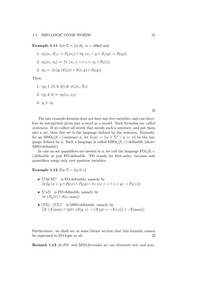
Example 1.11 Let Σ = {a, b}, w = abbab and
1. φ1(x1, X1) := Pa(x1) ∧ ∀y (x1 < y ∧ X1(y) → Pb(y))
2. φ2(x1, x2) := ∃z (x1 < z ∧ z < x2 ∧ Pb(z))
3. φ3 := ∃x∃y (Pa(x) ∧ S(x, y) ∧ Pb(y))
Then:
1. (w, 1, {2, 3, 4}) 6|= φ1(x1, X1)
2. (w, 2, 4) |= φ2(x1, x2)
3. w |= φ3
£
The last example-formula does not have any free variables, and can there-fore be interpreted given just a word as a model. Such formulas are calledsentences. If we collect all words that satisfy such a sentence, and put theminto a set, then this set is the language defined by the sentence. Formally,for an MSOΣ[S, <]-sentence φ, let L(φ) := {w ∈ Σ+ | w |= φ} be the lan-guage defined by φ. Such a language is called MSOΣ[S, <]-definable (short:MSO-definable).
In case no set quantifiers are needed in φ, we call the language FOΣ[S, <]-definable or just FO-definable. FO stands for first-order, because nowquantifiers range only over position variables.
Example 1.12 For Σ = {a, b, c}
• Σ∗ba∗bΣ∗ is FO-definable, namely by∃x∃y (x < y ∧ Pb(x) ∧ Pb(y) ∧ ∀z ((x < z ∧ z < y) → Pa(z)))
• Σ∗aΣ is FO-definable, namely by∃x (Pa(x) ∧ S(x,max))
• (ΣΣ) · (ΣΣ)∗ is MSO-definable, namely by∃X (X(min) ∧ ∀y∀z (S(y, z) → (X(y) ↔ ¬X(z))) ∧ ¬X(max))
Furthermore, we shall see in some future section that this formula cannotbe expressed in FO-logic at all. £
Remark 1.13 In FO- and MSO-formulas we can eliminate min and max.

16 CHAPTER 1. AUTOMATA AND LOGICAL SPECIFICATIONS
Example 1.14 Instead of
∃x (Pa(x) ∧ S(x,max))
we write∃x (Pa(x) ∧ ∃y (S(x, y) ∧ ¬∃z S(y, z)))
£
In general, substitute ψ(max), by:
∃y(ψ(y) ∧ ¬∃z y < z) .
Analogously for min.
Remark 1.15 In MSO-formulas we can eliminate <.Proof: Replace x < y by
∃X[¬X(x) ∧ ∀z∀z′ (X(z) ∧ S(z, z′) → X(z′)) ∧ X(y)
]
Example 1.16 Some more examples over Σ = {a, b, c}:
1. {w ∈ Σ+ | in w every a is followed only by a’s, until a b occurs} isdefinable by:
∀x(Pa(x) → ∃y
(x < y ∧ Pb(y) ∧ ∀z (x < z ∧ z < y → Pa(z))
))
2. a+ is definable by ∀x Pa(x).
3. a(ba)∗ is definable by
Pa(min)∧∀x∀y(S(x, y) → (Pa(x) → Pb(y))∧(Pb(x) → Pa(y))
)∧Pa(max)
£
1.2 The Equivalence Theorem
Now that we have defined the logic we are going to use, we shall present a wayto translate any given automaton to a formula of this logic and vice versa.To this purpose we do the following preparation: A formula φ(X1, . . . , Xn)is interpreted on word models (w, K1, . . . , Kn) with Ki ⊆ dom(w). The setKi of positions serves as an interpretation of Xi. To code such models bywords that can be processed by an automaton we collect for every positionk ∈ dom(w) the information if k ∈ K1, k ∈ K2, . . . , k ∈ Kn in the form ofa bit vector. Formally, we represent a word b1 . . . bm with sets of positionsK1, . . . , Kn by a word over the alphabet Σ × {0, 1}n:

1.2. THE EQUIVALENCE THEOREM 17
b1
(c1)1...
(c1)n
b2
(c2)1...
(c2)n
. . .
bm
(cm)1...
(cm)n
and we set (ck)j = 1 iff k ∈ Kj .
Example 1.17 Let Σ = {a, b}, w = abbab, K1 = ∅, K2 = {2, 4, 5} andK3 = {1, 2}.
wK1
K2
K3
a001
b011
b000
a010
b010
£
Theorem 1.18 (Buchi, Elgot, Trakhtenbrot 1960) A language L ⊆ Σ+
is regular if and only if it is MSO-definable. The transformation in both di-rections is effective.
For the proof we present regular languages by NFAs. Let us give anexample first.
Example 1.19 Given the following automaton A:
1
a,b
b2
b3
a,b
we have to construct a sentence φA with
w |= φA iff w ∈ L(A) .
In other words, φA has to express that there exists an accepting run of Aon w. To this purpose, along with φA we assume the existence of three setsX1, X2, X3, such that:
Xi = set of positions, at which A is in state i.
Example 1.20 abbab. An accepting run for this word is 112333. We encodeX1, X2, X3 in the following way (without the last state):
w : a b b a b
X1 : 1 1 0 0 0X2 : 0 0 1 0 0X3 : 0 0 0 1 1
£

18 CHAPTER 1. AUTOMATA AND LOGICAL SPECIFICATIONS
Naturally the automaton can only be in one state at each point of time.Therefore there is just one 1 in every column of the run. How can we describea successful run? That is, how do we set constraints to X1, . . . , Xn? Theformula we are looking for is a conjunction over 4 basic properties:
φA := ∃X1∃X2∃X3
[“X1, X2, X3 form a Partition”
∧ X1(min)
∧ ∀x∀y (S(x, y) → “at x, y one of the transitions is applied”
∧ “at max the last transition leads to a final state”]
Now let us explain each one of these properties (except the second, which isobvious) and give the respective MSO-formulas.
• “X1, X2, X3 form a Partition”: Partition is an expression for the abovementioned unambiguity of the automaton state. Since there is just one1 in every X-bitvector, X1, X2, X3 have to form a partition of dom(w).In terms of MSO-logic, we write:
∀x (X1(x) ∨ X2(x) ∨ X3(x))
∧ ¬∃x (X1(x) ∧ X2(x))
∧ ¬∃x (X2(x) ∧ X3(x))
∧ ¬∃x (X1(x) ∧ X3(x))
• “at x, y one of the transitions is applied”: In other words, we need aformula to represent the whole transition relation ∆:
(X1(x) ∧ Pa(x) ∧ X1(y)) ∨ (X1(x) ∧ Pb(x) ∧ X1(y)) ∨(X1(x) ∧ Pb(x) ∧ X2(y)) ∨ (X2(x) ∧ Pb(x) ∧ X3(y)) ∨(X3(x) ∧ Pa(x) ∧ X3(y)) ∨ (X3(x) ∧ Pb(x) ∧ X3(y))
• “at position max the last transition leads to a final state”: Since wewant the formula to be true if and only if the word is accepted by theautomaton, we have to force that the run on w ends in a final state ofA:
(X2(max)∧ Pb(max))∨ (X3(max)∧ Pa(max))∨ (X3(max)∧ Pb(max))
£
Proof of Theorem 1.18: Let A = ({1, . . . , m}︸ ︷︷ ︸
Q
, Σ, 1, ∆, F ) be an NFA. The
formula expressing that there exists a successful run of A on a word w ∈ Σ+
is then given by
φA = ∃X1 . . .∃Xm
[∀x
(X1(x) ∨ . . . ∨ Xm(x)
)∧ ∧
i6=j ¬∃x(Xi(x) ∧ Xj(x)
)

1.2. THE EQUIVALENCE THEOREM 19
∧ X1(min)
∧ ∀x∀y (S(x, y) → ∨
(i,a,j)∈∆ (Xi(x) ∧ Pa(x) ∧ Xj(y)))
∧ ∨
(i,a,j)∈∆,j∈F (Xi(max) ∧ Pa(max))]
Then A accepts w iff w |= φA.
Remark 1.21 φA does not contain any universal quantifiers over set vari-ables but only existential ones. Such an MSO-formula, namely of the form
∃X1 . . .∃Xmψ(X1, . . . , Xm)
where ψ does not contain any set quantifiers at all, is called an existentialMSO-formula (EMSO-formula).
Remark 1.22 For m states, dlog2(m)e set quantifiers suffice.
Example 1.23 In the case of 4 states: Instead of the sets X1, . . . , X4 itsuffices to use X1, X2 along with the convention that the states 1, . . . , 4correspond to the column vectors
(00
),(01
),(10
),(11
), respectively. £
Suppose now that we are given an MSO-formula φ and want to constructan NFA Aφ such that L(Aφ) = L(φ). The main idea is to proceed byinduction on the construction of φ(x1, . . . , xm, X1, . . . , Xn).
First we show how to eliminate the first-order variables xi and get equiv-alent formulas containing only set variables. To this purpose we representthe element x by the set {x} and then work with formulas of the formφ(X1, . . . , Xn). We call such formulas MSO0-formulas. Atomic MSO0-formulas are:
• X ⊆ Y and X ⊆ Pa
• Sing(X) (“X is a singleton set”)
• S(X, Y ) (“X = {x}, Y = {y} and S(x, y)”)
• X < Y (“X = {x}, Y = {y} and x < y”)
As usual, formulas are built up using ¬, ∨, ∧, →, ↔, ∃, and ∀.
Lemma 1.24 (MSO0-Lemma) Every MSO-formula φ(X1, . . . , Xn) is (overword models) equivalent to an MSO0-formula.
Proof: We proceed by induction over the structure of the given MSO-formula. In some of the intermediate steps we have to handle formulaswith free first-order (element) variables. As described above we transformthese variables into singleton set variables. More formally, by induction over

20 CHAPTER 1. AUTOMATA AND LOGICAL SPECIFICATIONS
the structure of an MSO-formula ψ(y1, . . . , ym, X1, . . . , Xn), we construct acorresponding MSO0-formula ψ∗(Y1, . . . , Ym, X1, . . . , Xn) with
(w, k1, . . . , km, K1, . . . , Kn) |= ψ iff (w, {k1}, . . . , {km}, K1, . . . , Kn) |= ψ∗
We omit the details. The idea is illustrated in the example below. 2
Example 1.25 For
φ(X1) = ∀x(Pa(x) → ∃y (S(x, y) ∧ X1(y))
)
construct
φ∗ = ∀X(Sing(X) ∧ X ⊆ Pa → ∃Y (Sing(Y ) ∧ S(X, Y ) ∧ Y ⊆ X1)
)
£
Corollary 1.26 To translate formulas φ(X1, . . . , Xn) to automata it suf-fices to consider MSO0-formulas.
A formula φ(X1, . . . , Xn) defines a language over the alphabet Σ×{0, 1}n.
Example 1.27 Let Σ = {a, b} and φ(X1) = ∀x(Pa(x) → ∃y (S(x, y) ∧
X1(y)))
(b0
)(a0
)(a1
)(b1
)satisfies φ
(b0
)(a0
)(a1
)(b0
)does not satisfy φ.
L(φ) = the set of words over Σ × {0, 1}, such that after every a in the firstcomponent there is a 1 in the second component. £
In the general case, for each φ(X1, . . . , Xn) we have to inductively con-struct a finite automaton over Σ × {0, 1}n. For the base case we considerthe atomic MSO0-formulas.
• X1 ⊆ X2:Given a word w ∈ (Σ × {1, 0}n)+, an automaton has to check thatwhenever the first component is 1, the second component is 1 as well.This is performed by the following NFA:
1
2
4
#00∗
3
5,
2
4
#01∗
3
5,
2
4
#11∗
3
5
that is, it accepts everything except
#10∗
, where # stands for arbitrary
letters in Σ and ∗ for arbitrary bit vectors in {0, 1}n−2.

1.2. THE EQUIVALENCE THEOREM 21
• X1 ⊆ Pa:
1»
a
0∗
–
,
»
a
1∗
–
,
»
6= a
0∗
–
• Sing(X1):
1
»
#0∗
–
»
#1∗
–
2
»
#0∗
–
• S(X1, X2):
1
2
4
#00∗
3
5
2
4
#10∗
3
5
2
2
4
#01∗
3
5
3
2
4
#00∗
3
5
• X1 < X2:
1
2
4
#00∗
3
5
2
4
#10∗
3
5
2
2
4
#00∗
3
5
2
4
#01∗
3
5
3
2
4
#00∗
3
5
For the induction step, we suppose that for the formulas φ1, φ2 thecorresponding NFAs A1, A2 are given and we only consider the connectors∨, ¬ and the quantifier ∃. The other operators (∧, →, ↔ and ∀) can beexpressed as a combination of the previous ones. Regarding the negation,¬φ1 is equivalent to the complement automaton of A1. As we know, we canconstruct it using the subset construction on A1 and then, in the resultingDFA, declare all states Q \ F as final ones. For the disjunction φ1 ∨ φ2 weconstruct the automaton that recognizes L(A1) ∪ L(A2). As usually we dothis by constructing the union automaton out of A1 and A2. To handle theexistential quantifier we need some preparation.
Lemma 1.28 (Projection Lemma) Let f : Σ → Γ be a projection ofthe alphabet Σ into the alphabet Γ extended to words by f(b1 . . . bm) :=f(b1) . . . f(bm). If L ⊆ Σ∗ is regular, then f(L) is regular as well.
Proof: Given an NFA A = (Q,Σ, q0, ∆, F ) that recognizes L, we constructthe NFA B = (Q,Γ, q0, ∆
′, F ) with ∆′ := {(p, f(a), q) | (p, a, q) ∈ ∆}. 2
22 CHAPTER 1. AUTOMATA AND LOGICAL SPECIFICATIONS
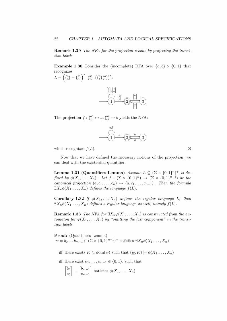
Remark 1.29 The NFA for the projection results by projecting the transi-tion labels.
Example 1.30 Consider the (incomplete) DFA over {a, b} × {0, 1} thatrecognizes
L =((
a0
)+
(b0
))∗ (b1
) ((a1
)(a1
))∗:
1
h
a
0
i
,h
b
0
i
h
b
1
i
2
h
a
1
i
3h
a
1
i
The projection f :(ac
)7→ a,
(bc
)7→ b yields the NFA:
1
a,b
b2
a3
a
which recognizes f(L). £
Now that we have defined the necessary notions of the projection, wecan deal with the existential quantifier.
Lemma 1.31 (Quantifiers Lemma) Assume L ⊆ (Σ × {0, 1}n)+ is de-fined by φ(X1, . . . , Xn). Let f : (Σ × {0, 1}n) → (Σ × {0, 1}n−1) be thecanonical projection (a, c1, . . . , cn) 7→ (a, c1, . . . , cn−1). Then the formula∃Xnφ(X1, . . . , Xn) defines the language f(L).
Corollary 1.32 If φ(X1, . . . , Xn) defines the regular language L, then∃Xnφ(X1, . . . , Xn) defines a regular language as well, namely f(L).
Remark 1.33 The NFA for ∃Xnϕ(X1, . . . , Xn) is constructed from the au-tomaton for ϕ(X1, . . . , Xn) by “omitting the last component” in the transi-tion labels.
Proof: (Quantifiers Lemma)w = b0 . . . bm−1 ∈ (Σ × {0, 1}n−1)+ satisfies ∃Xnφ(X1, . . . , Xn)
iff there exists K ⊆ dom(w) such that (w, K) |= φ(X1, . . . , Xn)
iff there exist c0, . . . , cm−1 ∈ {0, 1}, such that[b0
c0
]
. . .
[bm−1
cm−1
]
satisfies φ(X1, . . . , Xn)

1.2. THE EQUIVALENCE THEOREM 23
iff b0 . . . bm−1 = f(u) for some u with
u |= φ(X1, . . . , Xn) , i.e. for some u ∈ L
iff b0 . . . bm−1 ∈ f(L)
2
Example 1.34 For the following formula we construct an equivalent au-tomaton.
ϕ = ∃X1
(X1(min)︸ ︷︷ ︸
ψ1(X1)
∧∀x∀y(S(x, y) → (X1(x) ↔ ¬X1(y)))︸ ︷︷ ︸
ψ2(X1)
∧∀z Pa(z)︸ ︷︷ ︸
ψ3(X1)
)
We suppose that we are directly given automata A1, A2, A3 for thesub-formulas ψ1(X1), ψ2(X1), ψ3(X1) respectively:
A1: 1
[ ∗1 ]
2 [ ∗∗ ]
A2: 1[ ∗1 ][ ∗0 ]
2[ ∗1 ]
3
[ ∗0 ]
A3: 1 [ a∗ ]
We consider the conjunctions directly (without eliminating them by us-ing negation and disjunction). A3 merely requires that only a’s occur inthe first component. Since A1 and A2 make no restrictions about the firstcomponent, we can intersect A3 with both of them by always replacing the∗ in the first component with an a:
A′1 : 1
[ a1 ]
2 [ a∗ ]
A′2 : 1
[ a1 ][ a
0 ]
2[ a1 ]
3
[ a0 ]
Since A′1 only requires that in the first position in the word model a 1
occurs in the second component, we form the intersection of A′1 and A′
2 byremoving the transition from 1 → 2. So for the formula ψ1(X1) ∧ ψ2(X1) ∧ψ3(X1) we get the following equivalent automaton:
A′1 ∩ A′
2 : 1[ a1 ]
2[ a1 ]
3
[ a0 ]

24 CHAPTER 1. AUTOMATA AND LOGICAL SPECIFICATIONS
The projection on Σ leads to the final automaton A:
1a
3a
2a
Obviously L(A) = a+, so a (better) equivalent automaton is:
1a
2
a
£
The BET-Theorem allows the transformation of an MSO-formula intoan equivalent automaton and vice versa. How effective are these transforma-tions? Let us focus on the computational effort (in terms of time complexity)that is needed to perform the first one, assuming that we are given the au-tomata for the atomic formulas. If each one of two NFAs A1, A2 has atmost n states, then the NFA recognizing the
• union language has at most 2n + 1 states (because we create a newinitial state and depending on the first letter that is read, the newautomaton branches to one of the two initial ones)
• intersection language has at most n2 states(because we have to construct the product automaton)
• complement language has at most 2n states (because we have to use thesubset construction and turn the given NFAs to DFAs before switchingfinal and non-final states)
• projection language has at most n states (because we use the sameautomata and omit one component)
Does this mean that the transformation requires exponential time withrespect to the number of states of the automata? Unfortunately not. Thefact that the projection may turn a DFA into an NFA and the fact thatconstructing the complement automaton requires to make an automatonfirst deterministic (subset construction) means that, whenever an alternationbetween negation and projection occurs (e.g. when a universal quantifieroccurs), an additional exponential burden is added to our computationaleffort. So, in the general case, if k is the number of logical operators inthe formula, then the number of states in the resulting automaton grows
like 22...2n }
k. The following theorem shows that we cannot hope a better
bound.

1.2. THE EQUIVALENCE THEOREM 25
Theorem 1.35 (Meyer, Stockmeyer 1971) There is no translation ofMSO-formulas ϕ to automata in which the number of states of the resultingautomaton can be bounded by a function of the form
22...2n }
k
with a constant k.
Empirical observation (MONA system of Basin, Klarlund):If each DFA that is produced by the translation as an intermediate resultis immediately minimized, then even in the case of long formulas the sizeof the automaton mostly remains moderate. But doesn’t minimization addanother computational burden? Not really, because we will see in the nextchapter that for the case of a DFA, minimization can be done efficiently.Consequently, the examples for an hyper-exponential growth are not typical.
Example 1.36 We give to the MONA system the following formula:
ϕ(X, Y, x) : “X \ Y = {0, 1, 2, 4}′′ ∧ ψ(x) ∧ ¬X(x)
with ψ(x) := ∃Z(Z(0) ∧ Z(x) ∧ ∀y(0 < y ≤ x →((Z(y) → ¬Z(y − 1)) ∧ (¬Z(y) → Z(y − 1)))
MONA input:
var2 X,Y;
X\Y = {0,4} union {1,2};
pred even(var1 x) = ex2 Z: 0 in Z & x in Z &
(all1 y: (0 < y & y <= x) =>
(y in Z => y-1 notin Z) &
(y notin Z => y-1 in Z));
var1 x;
even(x) & x notin X;
The resulting automaton is (MONA output)

26 CHAPTER 1. AUTOMATA AND LOGICAL SPECIFICATIONS
9
0 1X 1X,X
2
10X
0 1
XXX
0 1 1X 0 1X,1,X
3
100
XXX
0 1 1X 0 1X,1,X
4
100
0 1 1X 0 1X,1,X
5
100
0 1 1X 0 11,X,1
6
0 1X 10,0
0 1 1X 0 1X,1,X
7
100
0 1 1X 0 11,X,1
8
0 1X 10,0
0X1
1 10 1X,1
0 1X 10,0
£
Now that we have connected automata to logic, we can make a compar-ison between them, as well as consider the applications of this connection.
• Automata: operational, formulas: descriptive
• Automata: implementation, formulas: specification
• Automata have local transitions, formulas have global operators (inparticular quantifiers)
• The semantics of automata are defined over the arbitrary construc-tion of state sequences, whereas the semantics of formulas are definedinductively (compositional)
• algorithmic questions on automata are often efficiently solvable, whereasthe ones on formulas are hard to solve (non-emptiness vs. satisfiabil-ity)
• For automata the minimization problem is approachable, for formulasit remains still incomprehensible.
How does all this relate to the “logic” of regular expressions? These canbe enriched by further operators that make them more convenient to usewithout increasing their expressive power. We add ∼ (for the complement)and ∩ (for the intersection).
Definition 1.37 Generalized regular expressions over Σ are built up byletters a ∈ Σ and ∅, ε by using +, ·,∩ (binary) and ∗,∼ (unary).
Example 1.38 The following property over words in Σ = {a, b, c}:

1.2. THE EQUIVALENCE THEOREM 27
“there are no two occurrences of b, between which only a’s occur, and atmost three c’s occur”
is defined by∼ (Σ∗ba∗bΣ∗) ∩ ∼ (Σ∗cΣ∗cΣ∗cΣ∗cΣ∗)
£
Remark 1.39 A language is definable by a generalized regular expressionif, and only if, it is regular.
For the definition of word sets (languages) generalized regular expressionsare an alternative to MSO-logic; they may be not so flexible, but in manycases they are much more convenient to use. Their translation into automatais of the same computational complexity as the translation of the formulas.
Remark 1.40 The BET-Theorem has been extended to other types of mod-els instead of finite words:
1. Automata on ω-words and their equivalence to MSO-logic (Buchi 1960)
2. Automata on finite trees and their equivalence to MSO-logic (Doner,Thatcher/Wright 1968)
3. Automata on infinite trees and their equivalence to MSO-logic (Rabin1969)
Application: Decidable theories. The initial motivation to reduce for-mulas to automata was “First-order arithmetics”, i.e. the first-order theoryof the structure (N, +, ·, 0, 1), which was proven to be undecidable (Godel1931). Based on this result Tarski formulated the following problem: Whatis the result if in its signature we keep only +1, but allow set quantifiers?
Corollary 1.41 (of the Buchi, Elgot, Trakhtenbrot Theorem) : Thesecond-order theory of the structure (N, +1) in which the second-order quan-tifiers range only over finite sets is decidable.
This theory is usually referred to as the weak second-order theory of onesuccessor (WS1S).
Theorem 1.42 The weak second-order theory of one successor (WS1S) isdecidable.
The use of tree automata and automata on infinite trees lead to furtherresults:
• The theory S1S refers to the structure (N, +1) with arbitrary set quan-tifiers.

28 CHAPTER 1. AUTOMATA AND LOGICAL SPECIFICATIONS
• The theory WS2S concerns the structure of the infinite binary tree(with two successor functions), in which the set quantifiers range onlyover finite sets.
• The theory S2S refers to the infinite binary tree with arbitrary setquantifiers.
All these theories are decidable using the corresponding automata and sim-ilar techniques as in the proof of Theorem 1.18.
1.3 Consequences and Applications in Model Check-ing
First of all, the Equivalence Theorem has a purely logical consequence:
Theorem 1.43 Every MSO-formula φ(X1, . . . , Xn) is over word modelsequivalent to an EMSO-formula, i.e. to a formula of the form
∃Y1 . . .∃Ymψ(X1, . . . , Xn, Y1, . . . , Ym)
where ψ is an FO-formula.
Proof: Use the BET-Theorem in both directions: φ ; Aφ ; ∃Y1 . . .∃Ym ψ.So, given an MSO-formula φ(X), we first construct the equivalent NFA
Aφ over the alphabet Σ × {0, 1}n and then transform it into an equivalentEMSO-formula ∃Y1 . . .∃Ym ψ. 2
Theorem 1.44 Satisfiability and equivalence of MSO-formulas over wordmodels are decidable problems.
Proof: Apply the transformations into automata:
• ϕ is satisfiable iff L(ϕ) 6= ∅ iff L(Aϕ) 6= ∅
• ϕ ≡ ψ iff L(ϕ) = L(ψ) iff L(Aϕ) = L(Aψ)
The constraints on the right can be tested algorithmically. 2
We look at the terminating behavior of finite state systems. The modelchecking problem is the following: Given a finite state system represented byan NFA A and a specification formulated as an MSO-formula φ, does everyword accepted by A satisfy the specification φ? This can be succinctlyrestated as “L(A) ⊆ L(φ)?”.
To solve the model checking problem we introduce error scenarios. Aword w is an error scenario if w ∈ L(A) but w 6|= φ, i.e. w ∈ L(A)∩L(A¬φ).

1.3. CONSEQUENCES AND APPLICATIONS IN MODEL CHECKING29
The solution of a model checking problem consists of two steps. Firstwe construct from a formula φ an automaton A¬φ using the BET-Theorem.Then we construct the product automaton B of A and A¬φ. B acceptsprecisely the error scenarios. Hence, we apply the emptiness test for B. IfL(B) turns out to be non-empty, then not every word accepted by A satisfiesthe specification φ. In this case the emptiness test returns a counter-exampleto φ, which can be used for debugging the system.
So, given an automaton A and an MSO-formula φ, to solve the modelchecking problem we have to do the following:
1. Construct the automaton A¬φ
2. Proceed to the product automaton A × A¬φ that recognizes L(A) ∩L(A¬φ).
3. Apply the non-emptiness test on the product automaton.
4. In case of non-emptiness, return a word that is accepted by the productautomaton (error scenario).
Example 1.45 MUX (Mutual exclusion) protocol modeled by a transitionsystem over the state-space B5.
Proc0: loop
(00) a0: Non_Critical_Section_0;
(01) b0: wait unless Turn = 0;
(10) c0: Critical_Section_0;
(11) d0: Turn := 1;
Proc1: loop
(00) a1: Non_Critical_Section_1;
(01) b1: wait unless Turn = 1;
(10) c1: Critical_Section_1;
(11) d1: Turn := 0;
A state is a bit-vector (b1, b2, b3, b4, b5) ∈ B5 (value of turn, line no. ofprocess 0, line no. of process 1). On this protocol we can define the systemautomaton AMutEx over the state space {0, 1}5, with initial state (00000),the alphabet B5 and the following transitions:
For process 0:
b1 0 0 b4 b5 → b1 0 1 b4 b51 0 1 b4 b5 → 1 0 1 b4 b50 0 1 b4 b5 → 0 1 0 b4 b5
b1 1 0 b4 b5 → b1 1 1 b4 b5b1 1 1 b4 b5 → 1 0 0 b4 b5
For process 1: analogously

30 CHAPTER 1. AUTOMATA AND LOGICAL SPECIFICATIONS
If we additionally label each transition with its target state, and declare allreachable states as final ones, the words being accepted by this automatonare exactly the system runs. Finally, for matters of system specification wecan represent the 5 bits by predicates X1, . . . , X5 and introduce abbreviatedcompact state properties that can be described by MSO-formulas:
ata0(t) := ¬X2(t) ∧ ¬X3(t) (states of the form (X00XX)Turn(t) = 0 := ¬X1(t) (states of the (0XXXX)
The first formula specifies all states where some part of the system is “ata0”, which means that process 0 is in line 00. The second one specifies allthose states where the value of the synchronization variable happens to be0. For the general case where state properties p1, . . . , pk are considered, aframework is used that is called Kripke structure.
Definition 1.46 A Kripke structure over propositions p1, . . . , pk has theform M = (S,→, s0, β) with
• a finite set S of states
• a transition relation →⊆ S × S (alternatively ⊆ S × Σ × S)
• an initial state s0
• a labeling function β : S → 2{p1,...,pn} assigning to each s ∈ S the setof those pi that are true in s
Usually, we write a value β(s) as a bit vector (b1, . . . , bn) with bi = 1 iffpi ∈ β(s).
Some very essential specifications of the MUX System would be thesafety condition and the liveliness condition. For the first we have to specifythat no state in which process 0 is in c0 and process 1 is in c1 will ever bereached:
ϕ := ∀x¬(atc0(x) ∧ atc1(x)
)
According to our model, we have to forbid all states of the form (X1010):
ϕ(X1, . . . , X5) = ∀x¬(X2(x) ∧ ¬X3(x) ∧ X4(x) ∧ ¬X5(x)
)
In the framework of model checking, this is an inclusion test, namely whetherevery (accepting) run of the finite system is also a (correct) model for theMSO-specification: L(AMutEx) ⊆ L(ϕ(X1, . . . , X5)).
For an example specification of the second kind, we require that “when-ever process 0 wants to enter the critical section (at b0), it will eventuallyindeed enter c0”:
∀x(atb0(x) → ∃y(x < y ∧ atc0(y))
)
The MSO formulation of this condition actually makes sense when it comesto infinite system runs, which goes beyond the scope of these course notes.
£

1.4. FIRST-ORDER DEFINABILITY 31
1.4 First-Order Definability
For the most cases of specification the expressive power of FO[S, <]-formulassuffices. A natural question to ask is what are the exact limits of this power,i.e. which regular languages can be expressed by FO-formulas. To thispurpose we are going to introduce two new formalisms, namely star-free(regular) expressions and the temporal logic LTL (“linear time logic”), andcompare them with FO-logic. Without giving a complete proof, we shallsee that all three formalisms define exactly the same class of languages.Finally, we will see that this class is a proper subset of the class of regularlanguages, i.e. there is a special class of languages that is regular (whichmeans MSO-definable) but not FO-definable.
1.4.1 Star-free Expressions
Definition 1.47 A star-free regular expression is a (generalized) regularexpression built up from the atoms ε, ∅, a ∈ Σ using only the operations · forconcatenation, + for union, ∩ for intersection, and ∼ for complementation.The language L(r) defined by such an expression r is also called star-free.
Example 1.48 Let Σ = {a, b, c}
1. Σ∗ is star-free, defined by ∼∅
2. a+ is star-free, defined by ∼ε ∩ ∼(Σ∗(b + c)Σ∗)
3. b(ab)∗ is star-free, defined by the constraint:“never c, begin with b, never aa nor bb, end with b”, i.e.:
∼(Σ∗cΣ∗) ∩ bΣ∗ ∩ ∼(Σ∗(aa + bb)Σ∗) ∩ Σ∗b
£
Remark 1.49
a. The use of complementation ∼ is essential.Indeed, complementation is the operation that enables us to representinfinite languages because by complementing a finite language we getan infinite one. With union, concatenation, and intersection we canonly produce finite languages starting from the finitely many symbolsof the alphabet.
b. The standard star-free expressions are produced out of a ∈ Σ, ε, ∅ byusing only + and ·; these expressions define exactly the finite lan-guages.
Theorem 1.50 Every star-free language L ⊆ Σ+ is FO-definable.

32 CHAPTER 1. AUTOMATA AND LOGICAL SPECIFICATIONS
This theorem follows from the more technical lemma below.
Lemma 1.51 For every star-free expression r there is an FO-formula ϕr(x, y)that expresses that “the segment from x up to y is in L(r)”, that is w ∈ L(r)iff w |= ϕr[min, max] for all w ∈ Σ+.
Proof: By induction on the construction of the star-free expression.Base cases:
• r = a: Set ϕr(x, y) := Pa(x) ∧ x = y
• r = ∅: Set ϕr(x, y) := ∃z(x ≤ z ∧ z ≤ y ∧ ¬(z = z))
Induction hypothesis: Let s, t be equivalent to ϕs(x, y), ϕt(x, y).Induction step: For r = s + t, r = s ∩ t and r = (∼s) ∩ ∼ε set:ϕr(x, y) := ϕs(x, y)∨ϕt(x, y), ϕs(x, y)∧ϕt(x, y), and ¬ϕs(x, y), respectively.For r = s · t we require the existence of two successive positions z, z′ thatare between x and y. From x up to z, ϕs holds, and from z′ up to y, ϕt
holds:
ϕr(x, y) := ∃z∃z′(x ≤ z ∧ z ≤ y ∧ x ≤ z′ ∧ z′ ≤ y ∧ϕs(x, z) ∧ S(z, z′) ∧ ϕt(z
′, y))
2
1.4.2 Temporal Logic LTL
The (propositional) temporal logic LTL (linear time logic) was first pro-posed in 1977 by A. Pnueli for purposes of system specification. Its mainadvantages are:
• variable-free compact syntax
• transformation into automata more efficiently than in the case of FO-formulas
• equivalence to FO[S, <]-logic
In this section we handle LTL only over finite words.
Definition 1.52 (LTL) Syntax: A temporal formula is built up frompropositional variables p1, p2, . . . using the connectives ¬,∨,∧,→,↔ andthe temporal operators X (next), F (eventually), G (always), and U (until).We write φ(p1, . . . , pn) for a temporal formula φ to indicate that at mostthe propositional variables p1, . . . , pn appear in φ.

1.4. FIRST-ORDER DEFINABILITY 33
Semantics: A temporal formula φ(p1, . . . , pn) is evaluated in a model (w, j)where 1 ≤ j ≤ |w| is a position in the word w, and w is of the form
w =
(b1(1)
...bn(1)
. . .
b1(|w|)...
bn(|w|)
)
The value bi(k) ∈ {0, 1} codes the truth value of proposition pi at positionk in w.
We define the semantics of temporal formulas as follows:
(w, j) |= pi iff bi(j) = 1|= Fφ iff ∃k (j ≤ k ≤ |w| and (w, k) |= φ)|= Gφ iff ∀k (j ≤ k ≤ |w| ⇒ (w, k) |= φ)|= Xφ iff j < |w| and (w, j + 1) |= φ
|= φUψ iff
{
∃k1(j ≤ k1 ≤ |w| and (w, k1) |= ψ
and ∀k (j ≤ k < k1 ⇒ (w, k) |= φ))
The Boolean connectives have the standard semantics.
Intuitively, (w, j) |= φ means that φ is satisfied at position j in the wordw. We write w |= φ for (w, 1) |= φ and define the language L(φ) acceptedby a temporal formula containing the propositional variables p1, . . . , pn tobe L(φ) = {w ∈ ({0, 1}n)+ | w |= φ}.
Example 1.53 The LTL-formula
ϕ := G(p1 → X(p1Up2))
expresses the following property:
“Whenever p1 holds, then from the next moment on the following holds:p1 holds until eventually p2 holds.”
Consider the model:
w =
[10
] [00
] [10
] [10
] [10
] [11
] [01
]
The formula holds on position 2, but not on position 1. Consequently, wewrite (w, 2) |= ϕ but w 6|= ϕ. £
Example 1.54
G(p1 → X(¬p2Up3))
expresses in (w, j) with w ∈ ({0, 1}3)+ the following property:

34 CHAPTER 1. AUTOMATA AND LOGICAL SPECIFICATIONS
“From position j onwards, whenever the first component is 1, then fromthe next position onwards the second component is 0, until at some
position the third component is 1”.
£
Example 1.55 Let n = 2 and w =
[10
] [00
] [11
] [01
] [10
] [01
]
• w |= G(p1 → Fp2), w 6|= G(p2 → Fp1)
• w |= X(¬p2Up1), w |= ¬p2Up1
• w 6|= p1U(p1 ∧ p2)
£
Theorem 1.56 Every LTL-definable language L ⊆ Σ+ is FO-definable.
Lemma 1.57 For every LTL-formula ϕ one can construct an equivalentFO[S, <]-formula ϕ∗(x) with
(w, j) |= ϕ iff (w, j) |= ϕ∗(x)
Proof: Inductive definition of ϕ∗(x):
• (pi)∗(x) := Xi(x)
• (¬ϕ)∗(x) := ¬(ϕ∗(x)), analogously for ∨,∧,→,↔
• (Gϕ)∗(x) := ∀y(x ≤ y → ϕ∗(y))
• (Fϕ)∗(x) := ∃y(x ≤ y ∧ ϕ∗(y))
• (Xϕ)∗(x) := ∃y(S(x, y) ∧ ϕ∗(y))
• (ϕUψ)∗(x) := ∃y(x ≤ y ∧ ψ∗(y) ∧ ∀z(x ≤ z ∧ z < y → ϕ∗(z))
)
2
Example 1.58
ϕ = G(p1 → X(¬p2Up3))ϕ∗(x) = ∀y(x ≤ y ∧ X1(y) → ∃z(S(y, z) ∧ ∃s(z ≤ s ∧ X3(s) ∧
∀t(z ≤ t ∧ t < s → ¬X2(t)))))
£
So far we have shown that:

1.5. BETWEEN FO- AND MSO-DEFINABILITY 35
• If L is star-free, then L is FO-definable.
• If L is LTL-definable, then L is FO-definable.
The converses also hold but won’t be proven in these course notes sincethis requires much bigger technical effort:
Theorem 1.59 (McNaughton 1969, Kamp 1968) The conditions “FO-definable”, “star-free”, and “LTL-definable” for a language L are equivalent.
1.5 Between FO- and MSO-definability
The question that arises now is whether there is an MSO-definable languagethat is not FO-definable. Using the above equivalences, this questions meansthat we are looking for regular languages that are not star-free. To thispurpose we introduce the “counting”-property, by which regular languagescan be distinguished from star-free ones. In particular, we show that:
• There is at least one regular language that is “counting”.
• Every star-free language is “non-counting”.
Definition 1.60 Call L ⊆ Σ+ non-counting if
∃n0 ∀n ≥ n0 ∀u, v, w ∈ Σ∗ : uvnw ∈ L ⇔ uvn+1w ∈ L.
This means for n ≥ n0 either all uvnw are in L, or none is.
Remark 1.61 The above condition is a strong pumping-property; namelyif for a sufficiently large n the segment vn occurs in a word of L, thenwe remain in L if we use higher powers of v. Furthermore, note that theposition of vn is arbitrary. The standard Pumping Lemma guarantees onlythe existence of a position to pump.
Definition 1.62 L is not non-counting (short: L is counting) iff
∀n0 ∃n ≥ n0 ∃u, v, w ∈ Σ∗ : (uvnw ∈ L ⇔ uvn+1w 6∈ L).
Example 1.63 • L1 = (aa)+ is counting: Given n0 take some evennumber n ≥ n0 and set u, w := ε, v := a. Then an ∈ L1, but an+1 /∈L1.
• L2 = b(a∗bb)∗ is counting: Given n0 take some even number n ≥ n0
and set u := b, v := b, w := ε. Then bbn ∈ L2, but bbn+1 /∈ L2.
• L3 = b(a+bb)∗ is non-counting because it is FO-definable by:
36 CHAPTER 1. AUTOMATA AND LOGICAL SPECIFICATIONS
Pb(min) ∧ Pb(max) ∧ ∀u(S(min, u) → Pa(u))∧∀x∀y( S(x, y) ∧ Pa(x) ∧ Pb(y) →
∃z(S(y, z) ∧ Pb(z) ∧ ∀u(S(z, u) → Pa(u)))) .
Theorems 1.65 and 1.59 imply that FO-definable languages are non-counting.
£
Remark 1.64 By “counting” we mean modulo-counting successive occur-rences of a particular pattern (the word v in the definition). L = a(ba)∗ isalso sort of a counting language since it contains only words of odd length,but it is not modulo-counting in the above sense.
Theorem 1.65 Every star-free language is non-counting.
Proof: By induction on the structure of star-free expressions.
Base cases: For a ∈ Σ, ∅, ε take n0 = 2 respectively. Then, for eachof these languages L, for each n ≥ n0, and for all u, v, w ∈ Σ∗ thefollowing holds:
uvnw ∈ L ⇔ uvn+1w ∈ L
Induction step “∼”: If for a suitable n0 and for every n ≥ n0
uvnw ∈ L ⇔ uvn+1w ∈ L
holds, then obviously this also holds for the complement of L.
Induction step “∩”: By induction hypothesis, for L1, L2 there are n1, n2,such that for all n ≥ ni
uvnw ∈ Li ⇔ uvn+1w ∈ Li (i = 1, 2)
Set n0 = max(n1, n2). Then for n ≥ n0 the following holds:
uvnw ∈ L1 ∩ L2 ⇔ uvn+1w ∈ L1 ∩ L2
Induction step “·”: Take the induction hypothesis as before and set n0 =2 · max(n1, n2) + 1. For n ≥ n0 consider uvnw ∈ L1 · L2. Considerthe decomposition of uvnw in two segments, uvnw = z1z2 with z1 ∈L1, z2 ∈ L2 as illustrated in Figure 1.2. By the choice of n0 one of thefollowing cases applies.
Case 1: z1 contains at least n1 v-segments. Then by induction hy-pothesis z′1 (with one v-segment more than z1) is in L1.Case 2: z2 contains at least n2 v-segments. Then by induction hy-pothesis z′2 (with one v-segment more than z2) is in L2.In both cases we get uvn+1w ∈ L1L2. The converse (from uvn+1w ∈L1L2 to uvnw ∈ L1L2) can be proven analogously. 2

1.5. BETWEEN FO- AND MSO-DEFINABILITY 37
n1 n2
vn
z1� L1 z2
� L2
u w
Figure 1.2: Illustration
Now that we distinguished these classes of languages on the level of logic,the natural thing to ask is whether there is a way to do the same on the levelof automata. That is, is there a property of automata that characterizes thestar-free expressions? This question is answered positively in Section 2.4.
In the following we introduce a finer complexity scale for (standard)regular expressions that refers to the number of occurrences of the staroperator, and relate this measure to a property of automata.
Definition 1.66 The star-height of a regular expression is defined induc-tively as follows:
• sh(a) = sh(∅) = sh(ε) = 0
• sh(r + s) = sh(r · s) = max(sh(r), sh(s))
• sh(r∗) = sh(r) + 1
For a regular Language L, the star-height of L is
sh(L) = min{n | there is a regular expression r with L = L(r) and sh(r) = n}
Remark 1.67 L is finite iff sh(L) = 0.
Theorem 1.68 (Eggan 1963) The star-height hierarchy is strict (over al-phabets with at least two letters): For each n ≥ 0 there exists a language Ln
with sh(Ln) = n.
For Ln we can take the family of languages, recognized by the following NFA(see exercises):
0 1 2 · · · 2n
a a a a
b b b b
The property of NFAs that corresponds to the star-height of expressions isthe “loop complexity” (also “feedback number”).

38 CHAPTER 1. AUTOMATA AND LOGICAL SPECIFICATIONS
Definition 1.69 The loop complexity lc(A) of an NFA A is the minimumnumber of steps of the following kind required to eliminate all loops of A:
“remove one state in each strongly connected component of the currenttransition graph”
Example 1.70 Verify that the following automaton has loop complexity 2:
0 1
2 3
1st step: Remove 12nd step: Remove 0 and 3
£
Example 1.71 lc(A1) = 1, lc(A2) = 2, and lc(A3) = 3.
A1 : 1a
a,b
2
a,b
1st step: Remove 1 and 2.
A2 : 1 21st step: Remove 1 (or 2)2nd step: Remove 2 (or 1)
A3 : 0 1 2 3
8 7 6 5 4
1st step: Remove 42nd step: Remove 2 and 63rd step: Remove 0 and 7
£
Analogously, we can define the loop complexity of a regular language.
Definition 1.72 The loop complexity of a regular language is
lc(L) = min{n | there exists an NFA A with L = L(A) and lc(A) = n}
Theorem 1.73 (Eggan 1963) For every regular language L, sh(L) = lc(L).
The proof is a refinement of the one for Kleene’s theorem (Theorem 1.4). Forfurther details, please refer to J.R. Buchi: Finite Automata, Their Algebrasand Grammars, Sect. 4.6.
Theorem 1.74 (Hashiguchi 1988) Given a regular language L (say de-fined by an NFA) the star-height can be calculated algorithmically.
For the case of generalized regular expressions the generalized star-heightgsh is defined analogously to the one of the standard star-height.

1.6. EXERCISES 39
Remark 1.75
• gsh(L) ≤ sh(L) (i.e. we may be able to reduce the star-height bysubstituting some stars by the extended operators of the generalizedregular expressions) but in general we cannot reduce it to 0 because
• gsh(L) = 0 iff L is star-free (by definition).
• There exist regular languages L with gsh(L) ≥ 1 (compare Exam-ple 1.63 on page 35).
Open problem (since 1971): Are there regular languages L with gsh(L) ≥2?
We suspect that in case there is a solution, it goes to the direction ofnesting modulo-counting since this is the identifying property of non-star-free expressions. We define the languages:
E = (00)∗1 (“even block”)O = (00)∗01 (“odd block”)
The suggestion of using the language
specifying an even number of even blocks (((O∗E)(O∗E))∗O∗) failed after afew years.
Theorem 1.76 (Thomas., Theor. Comput. Sci. 13 (1981))
gsh(((O∗E)(O∗E))∗E∗) = 1
Another proposed language L as candidate for a language with gsh(L) =2 was (O+E+O+E+)∗. Also for this language it was later proven thatgsh(L) = 1. For details, please refer to M. Robson, More languages ofgeneralized star height 1, Theor. Comput. Sci. 106 (1992), 327-335.
1.6 Exercises
Exercise 1.1 Give FO- or MSO-formulas for the languages that are definedby the following regular expressions or descriptions in colloquial language:
(a) a+b∗,
(b) aab∗aa,
(c) there are at least three occurrences of b, and before the first b there areat most two occurrences of a.
Exercise 1.2 Consider the following NFA A:
1b
2
a
4
b
3 ab

40 CHAPTER 1. AUTOMATA AND LOGICAL SPECIFICATIONS
In the lecture it was shown how to construct an equivalent formula ϕA withfour set variables X1, · · · , X4. According to the hint of the lecture, give aformula with only two set variables. (The states 1, 2, 3, 4 should correspond
to the vectors
[00
]
,
[01
]
,
[10
]
,
[11
]
). Is L(A) FO-definable?
Exercise 1.3 (a) For the MSO-formula
∃x∀y(x < y → Pa(y))
give an equivalent MSO0-formula.
(b) Let Σ = {a, b}. The following MSO0-formula defines a language overΣ × {0, 1}3. Give (by direct construction) an equivalent NFA.
(X1 ⊆ X2) ∧ (X1 < X3) ∧ (X3 ⊆ Pa) .
Exercise 1.4 ∗ Show that every regular language L ⊆ Σ+ is definable by anEMSO-sentence with only one single set quantifier.
Exercise 1.5 Let Σ = {a, b} and
ϕ(X1, y) :=(¬Pa(y) → X1(y)
),
ψ(X1) := ∀y ϕ(X1, y) and
χ := ∃X1 ψ(X1).
(a) Write ϕ as an MSO0-formula ϕ(X1, Y ).
(b) Construct an NFA over Σ × {0, 1}2 recognizing L(ϕ(X1, Y )).
(c) Using (b) construct an NFA over Σ × {0, 1} recognizing L(ψ(X1)).
(d) Using (c) construct an NFA over Σ recognizing L(χ).
Exercise 1.6 Consider the following two decidability problems:
(a) Given an MSO-sentence ϕ, does ϕ hold for all nonempty word models?
(b) Given an MSO-sentence ϕ, does ϕ hold for all nonempty word modelsof even length?
Describe algorithms for solving these problems.
Exercise 1.7 Consider the word model
w :=
[1 0 1 0 1 00 0 1 1 0 1
]
and the formulas

1.6. EXERCISES 41
1. ϕ = p2U(p1 ∧ ¬p2) and
2. ψ = G(p1 → Xp2)
(a) For each j = 1, · · · , 6 answer whether the formulas hold in (w, j) or not.
(b) Give equivalent FO-formulas and star-free expressions.
Exercise 1.8 ∗ For n ≥ 1 let An be the following NFA:
0a
1b
a
2b
· · ·a
nb
(a) Show that L(An) is star-free.
(b) Show that for L(A2n) there exists a conventional regular expression (i.e.only using +, ·,∗) of star-height n.(The star-height of an expression is the maximal number of nested stars.Example: (a(aa)∗ + (bb)∗)∗ has star-height 2)
(c) Give an LTL-formula for L(An).
Hint: For (a),(b) it is useful, to consider next to An also the automataA+
n , A−n ; A+
n has initial state 0, final state n, A−n has initial state n, final
state 0.
Exercise 1.9 Give star-free expressions for the languages defined by the
following LTL-formulas. The alphabet is Σ =
{[00
]
,
[01
]
,
[10
]
,
[11
]}
. Write[1∗
]
for
[10
]
+
[11
]
, etc.
(a) XX(p1 ∧ G¬p2)
(b) FG(p1 ∧ ¬Xp2)
(c) F (p1 ∧ X(¬p2Up1))
Exercise 1.10 Decide whether the following languages are “counting” andverify your assumption.
(a) b(abb)∗
(b) a(bbb)∗aa

42 CHAPTER 1. AUTOMATA AND LOGICAL SPECIFICATIONS

Chapter 2
Congruences andMinimization
In this chapter we are interested in reducing the size of automata whilekeeping their functionality. For finite automata (on words or on trees) thesize usually refers to the number of states. The states of an automaton or asystem represent the distinctions that are made in order to fulfill a certaintask. The goal is to make this number of distinctions as small as possible.For this purpose we now take the graph theoretic view (as opposed to thelogical view from the previous chapter) of automata. As we will see, thereare elegant techniques that allow us to compare and improve automata onthe system level, rather than on the specification level.
2.1 Homomorphisms, Quotients and Abstraction
There are cases in the analysis and design of a system, where we are inter-ested only in a rough view of its structure and want to spare ourselves thelocal details. In this case, we actually represent by a model only the topol-ogy and interconnection between the subsystems and abstract away fromtheir own functionality.
Example 2.1 The NFA A2 on the right-hand side of Figure 2.1 is a roughview on the NFA A2 on the left-hand side, where the subsystem of the states1, 2, and 3 (counting a’s modulo 3) is represented by state B. This mergingof states corresponds to the following homomorphism:
0 7→ A, 1 7→ B, 2 7→ B, 3 7→ B
£
Definition 2.2 Let A = (A, RA, fA, cA),B = (B, RB, fB, cB) be two struc-tures, with
43

44 CHAPTER 2. CONGRUENCES AND MINIMIZATION
0 1
2
3
A Bb
a
a
a
b
b
b
a
Figure 2.1: Merging states in an NFA
• universes A, B,
• binary relations RA ⊆ A × A, RB ⊆ B × B,
• binary functions fA : A × A → A, fB : B × B → B and
• distinguished elements (“constants”) cA ∈ A, cB ∈ B.
A homomorphism from A to B is a function h : A → B with
• for x1, x2 ∈ A: If (x1, x2) ∈ RA, then (h(x1), h(x2)) ∈ RB
• for x1, x2 ∈ A: h(fA(x1, x2)) = fB(h(x1), h(x2))
• h(cA) = cB
The definition is analogous for relations and functions of other arity.
Example 2.3 The “Parikh-mapping”:A = ({a, b}∗, ·, ε), B = (N × N, +, (0, 0))h(w) = (|w|a, |w|b) (Numbers of a’s and b’s in w)E.g.: h(aabab) = (3, 2)The function h is a homomorphism because:
• for w1, w2 ∈ {a, b}∗: h(w1 · w2) = (|w1 · w2|a, |w1 · w2|b) = (|w1|a +|w2|a, |w1|b + |w2|b) = (|w1|a, |w1|b) + (|w2|a, |w2|b) = h(w1) + h(w2)
• h(ε) = (|ε|a, |ε|b) = (0, 0)
£
Example 2.4 Consider again the NFAs A1 and A2 from Figure 2.1:
({0, 1, 2, 3}, 0, R1a, R
1b , {1}) with
R1a = {(1, 2), (2, 3), (3, 1)} and
R1b = {(0, 0), (0, 1)}
({A, B}, A, R2a, R
2b , {B}) with
R2a = {(B, B)} and
R2b = {(A, A), (A, B)}

2.1. HOMOMORPHISMS, QUOTIENTS AND ABSTRACTION 45
The domain of this homomorphism h is the state set of A1 and has thefollowing discrete values: h(1) = h(2) = h(3) = B, h(0) = A. It is indeed ahomomorphism, because every transition from R1
a is mapped to a transitionin R2
a. Analogously for R1b and R2
b . £
Definition 2.5 Let A1 = (Q1, Σ, q10, ∆
1, F 1) and A2 = (Q2, Σ, q20, ∆
2, F 2)be NFAs. An NFA-homomorphism from A1 to A2 is a function h : Q1 → Q2
with
• h(q10) = q2
0
• (p, a, q) ∈ ∆1 ⇒ (h(p), a, h(q)) ∈ ∆2
• q ∈ F 1 ⇒ h(q) ∈ F 2
Remark 2.6 This is covered also by the general definition of homomor-phism if ∆1 is decomposed into binary relations R1
a for each a ∈ Σ with:
(p, q) ∈ R1a iff (p, a, q) ∈ ∆1
and analogously for ∆2.
Remark 2.7 Let h be an NFA-homomorphism from A1 to A2. Then thefollowing holds: If A1 accepts the word w, then so does A2. Hence, L(A1) ⊆L(A2). In other words abstraction by homomorphism produces an NFA thatrecognizes a super-language of the one defined by the initial NFA.
Example 2.8 Consider A1 and A2 from Example 2.4:
L(A1) = b+(aaa)∗
L(A2) = b+a∗
£
Remark 2.9 An NFA-homomorphism h of A yields a matching (or equiv-alence) of the states of A: p, q are h-equivalent iff h(p) = h(q). In shortterms: A homomorphism yields a state equivalence.
The converse of Remark 2.9 also holds, namely: A state equivalenceyields a homomorphism. To this purpose we consider a partitioning of thestates of the NFA A = (Q,Σ, q0, ∆, F ) and we write p ∼ q if p, q are in thesame class q/∼ = {p ∈ Q | p ∼ q} (i.e. they are “equivalent”).
Definition 2.10 The quotient automaton A/∼ of A is defined by A/∼ =(Q/∼, Σ, q0/∼, ∆/∼, F/∼) with
• Q/∼ = set of ∼-classes q/∼ for q ∈ Q
46 CHAPTER 2. CONGRUENCES AND MINIMIZATION
• (P, a, R) ∈ ∆/∼ iff there is p ∈ P, r ∈ R with (p, a, r) ∈ ∆, for∼-classes P, R
• P ∈ F/∼ iff there exists p ∈ P with p ∈ F
Then: h : q 7→ q/∼ is a homomorphism from A to A/∼.
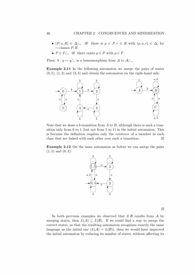
Example 2.11 In the following automaton we merge the pairs of states(0, 5), (1, 2) and (3, 4) and obtain the automaton on the right-hand side.
0 1 2
345
b
aa
a
a
a
a
b b
bb
A B
C
b
aa
a a, b
a, b
Note that we draw a b-transition from A to B, although there is such a tran-sition only from 0 to 1 (but not from 5 to 1) in the initial automaton. Thisis because the definition requires only the existence of a member in eachclass that are linked with each other over such a transition. £
Example 2.12 On the same automaton as before we can merge the pairs(1, 5) and (0, 4):
0, 4
1, 5 2
3
a, b a
a
a
a
b b
bb
£
In both previous examples we observed that if B results from A bymerging states, then L(A) ⊆ L(B). If we could find a way to merge thecorrect states, so that the resulting automaton recognizes exactly the samelanguage as the initial one (L(A) = L(B)), then we would have improvedthe initial automaton by reducing its number of states, without affecting its

2.1. HOMOMORPHISMS, QUOTIENTS AND ABSTRACTION 47
functionality. Furthermore, the best possible merging of states would leadus to an equivalent automaton with the minimum number of states. This iswhat we call the minimization problem of NFAs; namely given an NFA A,to find an equivalent NFA B that has the minimum number of states. Butcan we really achieve this by merging states? The following two examplesgive an answer to this question.
Example 2.13 Let A be an NFA and call Aq the same NFA as A but witha different initial state, namely q. To minimize A we suggest to merge twostates p, q, if L(Ap) = L(Aq). That is, if A accepts the same language bothstarting from p and from q, then we shall merge p and q.
A
B
C
b
a
b
a, b
In the automaton above there is no pair that can be merged in way describedbefore:
• A vs. C: From A, b is accepted, from C not,
• A vs. B: From B, ε is accepted, from A not,
• B vs. C: From B, ε is accepted, from C not.
But still, it is obvious that the automaton can be minimized since states Aand B suffice to accept the same language, namely Σ∗b. £
Unfortunately, things are even worse since there are cases where evenif we try all possible mergings (without following a specific rule as in theprevious example), we will not find the minimal NFA.
Example 2.14 Consider the language L = Σ∗aΣ, over Σ = {a, b}. Obvi-ously the minimal automaton A that recognizes L is the following:
a a, b
a, b
Another (not minimal) automaton B recognizing L is the following:

48 CHAPTER 2. CONGRUENCES AND MINIMIZATION
1 2
3
4
a
b
a
a
b
b
b
a
We observe that there is no proper quotient automaton of B that recognizesL. This means that in the general case of the minimization of an NFA itdoes not suffice to merely merge the existing states. £
2.2 Minimization and Equivalence of DFAs
We first look at the minimization problem for DFAs. In this case we cansuccessfully apply the techniques that we studied in the previous sectionand furthermore we have an efficient algorithmic solution. Before starting,we have to adopt a more abstract view on DFAs, namely consider them asalgebras.
Definition 2.15 Let Σ = {a1, . . . , an}. A DFA A = (Q,Σ, q0, δ, F ) canbe represented as a structure A = (Q, q0, δa1 , . . . δan , F ) with δai
: Q → Q,defined by δai
(p) := δ(p, ai). This is an algebra with a distinguished subsetF .
Every word w = b1 . . . bm induces a function δw : Q → Q, which isdefined as a composition of δb1 , . . . , δbm
: δw(p) = δbm(δbm−1(. . . δb1(p) . . .)).
A accepts w iff δw(q0) ∈ F .
We are going to apply the homomorphisms on the structures A.
Example 2.16
1 2
34
b
b
b
b
aa aa A Bb
b
a a
Looking at the automaton on the right-hand side we observe that with a weremain at the same state, whereas with b we switch from A to B and viceversa. So, δ2
a is the identity function and δ2b is the permutation A 7→ B, B 7→
A.
To the automaton on the left-hand side we apply a homomorphism hdefined by h(1) = h(4) = A, h(2) = h(3) = B. To ensure that it is indeed a

2.2. MINIMIZATION AND EQUIVALENCE OF DFAS 49
homomorphism we have to check for each p ∈ {1, 2, 3, 4} the homomorphismcondition:
h(δ1a(p)) = δ2
a(h(p)), h(δ1b (p)) = δ2
b (h(p))
or in standard syntax:
h(δ1(p, x)) = δ2(h(p), x) for x ∈ Σ .
£
Next, we adapt the definition of NFA-homomorphism introduced in theprevious section to the case of DFAs.
Definition 2.17 Let A1 = (Q1, Σ, q10, δ
1, F 1) and A2 = (Q2, Σ, q20, δ
2, F 2)be DFAs. A DFA-homomorphism from A1 to A2 is a homomorphism h :Q1 → Q2 between the corresponding algebras. This means:
• h(q10) = q2
0
• h(δ1(p, a)) = δ2(h(p), a)
• h(F 1) ⊆ F 2
If h is a bijective function and h(F 1) = F 2, then h is called an isomorphism.
Example 2.18 From the left automaton we proceed to the right one bymerging 1 with 3 and 2 with 4.
0 1 2
34
b a
a
a
a
a b b
bb
A B Cb
a
a
a b b
This corresponds to a homomorphism h with: h(0) = A, h(1) = h(3) = B,h(2) = h(4) = C. This homomorphism is also a DFA-homomorphism,because both the initial and the resulting automata are DFAs. £
Example 2.19 On the same automaton as in the previous example wemake a different merging of states, namely 1 with 2 and 3 with 4.

50 CHAPTER 2. CONGRUENCES AND MINIMIZATION
0 1 2
34
b a
a
a
a
a b b
bb
A B
C
b
aa
a a, b
a, b
The mapping h(0) = A, h(1) = h(2) = B, h(3) = h(4) = C yields anNFA-homomorphism, but not a DFA-homomorphism. We observe that ifwe want to preserve determinism in the resulting automaton, we cannotmerge any pairs of states, even if this adheres to the conditions of the NFA-homomorphism. There must be some additional relation between the twostates before they are merged. £
Remark 2.20 Every DFA-homomorphism induces an NFA-homomorphism;the converse does not hold. This means that if a DFA-homomorphism fromA to B exists, then L(A) ⊆ L(B) holds (as a result of the induced NFA-homomorphism).
Remark 2.21 A partitioning of states with a corresponding equivalence ∼defines a DFA-homomorphism iff ∼ is a congruence with respect to thetransition functions δa for each a ∈ Σ and preserves the distinction betweenfinal and non-final states. Formally:
p ∼ q ⇒ δa(p) ∼ δa(q)
and p ∼ q ⇒ (p ∈ F ⇔ q ∈ F )
Definition 2.22 A DFA-homomorphism from A = (Q,Σ, q0, δ, F ) to B de-fines a quotient-DFA of A in the following way: We set p ∼ q iff h(p) = h(q)and define A/∼ = (Q/∼, Σ, q0/∼, δ/∼, F/∼) with
• Q/∼ = the set of ∼-classes q/∼ for q ∈ Q
• δ/∼(p/∼, a) = δ(p, a)/∼• p/∼ ∈ F/∼ iff p ∈ F
Explanation: The definition of δ/∼(p/∼, a) is independent of the represen-tative p. This goes also for F/∼.
Definition 2.23 For a DFA A = (Q,Σ, q0, δ, F ), where w.l.o.g. we supposethat all states are reachable from q0 we define p ∼A q, if L(Ap) = L(Aq).Equivalently:
δw(p) ∈ F iff δw(q) ∈ F for all w ∈ Σ∗ .

2.2. MINIMIZATION AND EQUIVALENCE OF DFAS 51
Remark 2.24 a) ∼A is a right congruence, i.e. an equivalence relationandif p ∼A q and a ∈ Σ, then δa(p) ∼A δa(q).
b) The DFA A/∼Ais called the reduced DFA of A, short Ared and L(A) =
L(Ared).
Definition 2.25 (Nerode congruence) Let L ⊆ Σ∗.
u ∼L v iff for all w ∈ Σ∗ uw ∈ L ⇔ vw ∈ L.
This means that for any future w, u and v need not be distinguished withrespect to L. We often use the negation of this equivalence to prove thattwo words belong in different equivalence classes, namely u 6∼L v iff thereexists some w with uw ∈ L and vw 6∈ L (or uw 6∈ L and vw ∈ L).
Example 2.26 Consider the language L = a(bb)∗. a and b are not equiva-lent: Take w = ε, then aw = a ∈ L but bw = b 6∈ L. a, abb, abbbb, . . . are forexample equivalent. ε, a, b, ab are pairwise not equivalent. £
Remark 2.27 ∼L is a right congruence with respect to concatenation, whichmeans that if u ∼L v, then ua ∼L va and generally uw ∼L vw.
Proof: Show that ua ∼L va, i.e. uay ∈ L ⇔ vay ∈ L for all y ∈ Σ∗:
uay ∈ L ⇔ u(ay) ∈ L ⇔ by assumption v(ay) ∈ L ⇔ vay ∈ L
Notation: For the ∼L-class of u we write [u]L or just [u].In a DFA A that recognizes L, we observe that if both u and v lead to
the same state, then u ∼L v. This holds because from δ(q0, u) = δ(q0, v)we imply δ(q0, uw) = δ(q0, vw) and consequently uw ∈ L ⇔ vw ∈ L. Thismeans that there can be at most that many ∼L-classes as there are states:
Remark 2.28 If a DFA A recognizes the language L, then:
Number of ∼L-classes ≤ number of A-states.
It follows that if L is regular, then ∼L has a finite index, i.e. there arefinitely many equivalence classes.
Definition 2.29 (Canonical DFA) Let L be a language with finiteindex(∼L). The canonical DFA AL = (QL, Σ, q0L, δL, FL) for L is definedas follows:
• QL := { [u]L | u ∈ Σ∗} the (finite) set of ∼L-classes,
• q0L := [ε],

52 CHAPTER 2. CONGRUENCES AND MINIMIZATION
• δL([u], a) := [ua] and
• FL := {[u] | u ∈ L}.
Example 2.30 Let L = {a, b}∗abb{a, b}∗. There are four different ∼L-classes: [ε]L, [a]L, [ab]L, [abb]L. Since
[ε]L = [b]L , [aba]L = [aa]L = [a]L , [abba]L = [abbb]L = [abb]L
we obtain the following canonical automaton for L:
[ε]La
b
[a]L
a
b
[ab]La
b[abb]L a,b
£
Proposition 2.31 The canonical automaton AL accepts L.
Proof: AL accepts w ⇔ δ(q0L, w) ∈ FL ⇔ [w]L ∈ FL ⇔ w ∈ L 2
AL has index(∼L) many states. So AL is a DFA accepting L with theminimum possible number of states. The following theorem shows that AL
is unique up to isomorphism.
Theorem 2.32 (Main DFA-Minimization Theorem) If the DFA A =(Q,Σ, q0, δ, F ) recognizes L, then the DFA Ared is isomorphic to AL.
Proof: We have to show that for Ared = (Q,Σ, q0, δ, F ) there is a bijectionf : Q −→ QL with f(q0) = q0L, f(F ) = FL and f(δ(q, a)) = δL(f(q), a).
Definition of f : Pick for any state q of Ared a word uq with δ(q0, uq) = qand let f(q) := [uq]L. Obviously f is an isomorphism between Ared and AL.
2
Example 2.33 Consider the following automaton, which is obviously theminimal one that can recognize the language L = a(bb)∗. To map thisautomaton to a canonical one, we choose the following isomorphism:
1 7→ [ε] 2 7→ [bab] = [b] 3 7→ [ab] 4 7→ [abb] = [a]
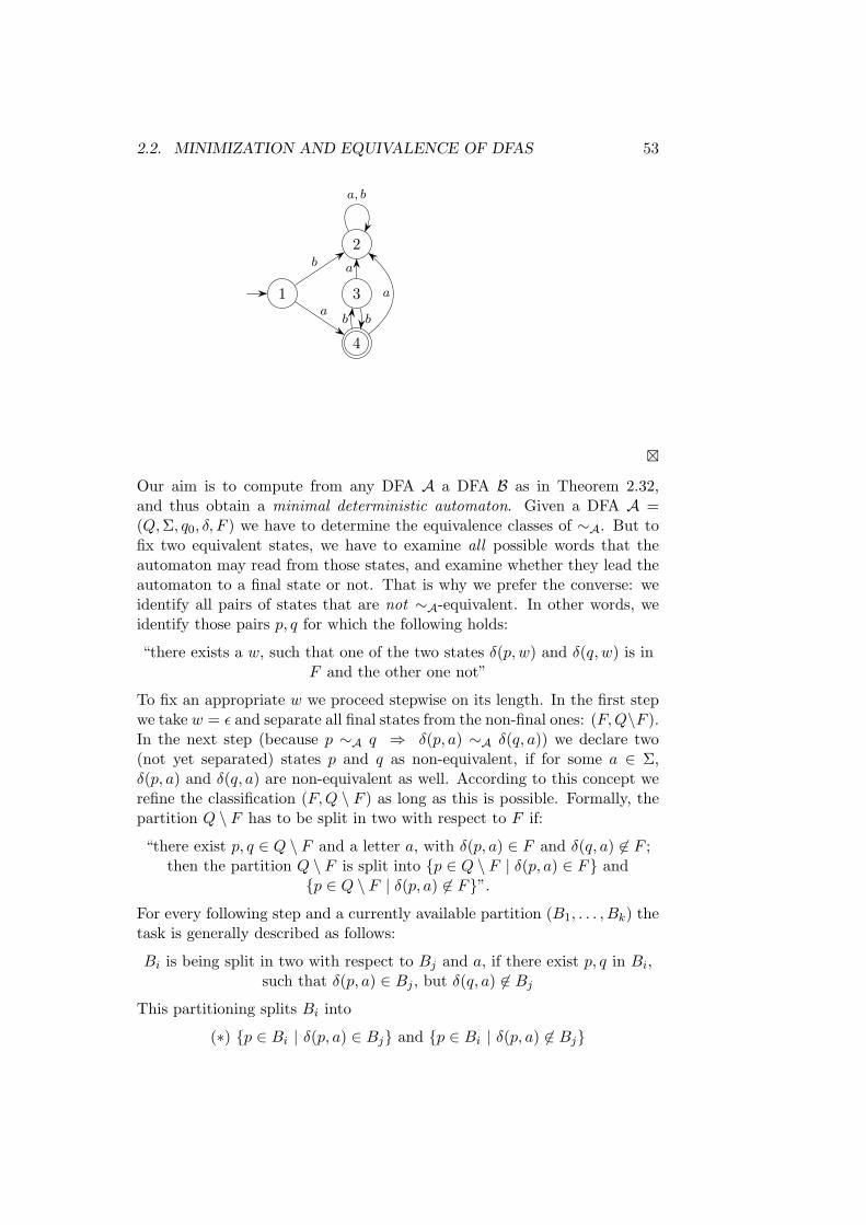
2.2. MINIMIZATION AND EQUIVALENCE OF DFAS 53
1
4
2
3
b
ab b
a
a
a, b
£
Our aim is to compute from any DFA A a DFA B as in Theorem 2.32,and thus obtain a minimal deterministic automaton. Given a DFA A =(Q,Σ, q0, δ, F ) we have to determine the equivalence classes of ∼A. But tofix two equivalent states, we have to examine all possible words that theautomaton may read from those states, and examine whether they lead theautomaton to a final state or not. That is why we prefer the converse: weidentify all pairs of states that are not ∼A-equivalent. In other words, weidentify those pairs p, q for which the following holds:
“there exists a w, such that one of the two states δ(p, w) and δ(q, w) is inF and the other one not”
To fix an appropriate w we proceed stepwise on its length. In the first stepwe take w = ε and separate all final states from the non-final ones: (F, Q\F ).In the next step (because p ∼A q ⇒ δ(p, a) ∼A δ(q, a)) we declare two(not yet separated) states p and q as non-equivalent, if for some a ∈ Σ,δ(p, a) and δ(q, a) are non-equivalent as well. According to this concept werefine the classification (F, Q \ F ) as long as this is possible. Formally, thepartition Q \ F has to be split in two with respect to F if:
“there exist p, q ∈ Q \ F and a letter a, with δ(p, a) ∈ F and δ(q, a) 6∈ F ;then the partition Q \ F is split into {p ∈ Q \ F | δ(p, a) ∈ F} and
{p ∈ Q \ F | δ(p, a) 6∈ F}”.
For every following step and a currently available partition (B1, . . . , Bk) thetask is generally described as follows:
Bi is being split in two with respect to Bj and a, if there exist p, q in Bi,such that δ(p, a) ∈ Bj , but δ(q, a) 6∈ Bj
This partitioning splits Bi into
(∗) {p ∈ Bi | δ(p, a) ∈ Bj} and {p ∈ Bi | δ(p, a) 6∈ Bj}

54 CHAPTER 2. CONGRUENCES AND MINIMIZATION
A CB
D E F G
a
b
b
a
a
b
a
a
b
b
b
a
b
a
AD CBG
E F
a
b
b
a
a
a
b
b
b
a
Figure 2.2: Partition refinement
Partition refinement algorithm:
1. Initialization: B1 = F, B2 = Q \ F
2. While there exist Bi, Bj , a with (∗), partition Bi with respect to Bj
and a.
Example 2.34 We want to find equivalence classes in the automaton fromthe left-hand side of Figure 2.2. The initial partition is (ABDEFG, C) andwe now stepwise split these blocks according to (∗):
1st step: Splitting ABDEFG w.r.t. C and b yields BG and ADEF .
2nd step: Splitting ADEF w.r.t. BG and a yields AD and EF .
3rd step: Splitting EF w.r.t. C and a yields E and F .
Q
initialization ABDEFG C
1st step BG ADEF
2nd step AD EF
3rd step E F
The resulting minimized automaton is shown on the right-hand side of Fig-ure 2.2. £

2.2. MINIMIZATION AND EQUIVALENCE OF DFAS 55
Complexity of the algorithm: There can be at most |Q|−1 splits. Everyloop requires at most to calculate δ(q, a) for q ∈ Q and a ∈ Σ (for checkingcondition (∗)). Altogether this sums up to O(|Σ| · |Q|2). We conclude thatthe minimization of a DFA can be done in second-order polynomial time withrespect to the number of states. This can be improved by the algorithm ofHopcroft, which requires only O(|Q| log |Q|) time.
Now that we know an efficient algorithm to minimize DFAs, we canuse it to construct an efficient equivalence test, according to the followingcorollary.
Corollary 2.35 (of the Main Minimization Theorem) Two DFAs overΣ are equivalent, if and only if the corresponding reduced automata are iso-morphic.
This means that we can use the following algorithm to check, whethertwo DFAs are equivalent:
1. Given two DFAs A,B construct their reduced versions Ared,Bred.
2. Starting from the initial state perform breadth-first search in Ared,Bred and name each reached state q with the smallest word that leadsto it, according to the canonical order.
3. Check whether the transition tables and the final states are identical.
Time complexity: O(n log n), like for the minimization.
Example 2.36 We consider the canonical automaton of Example 2.33 andapply the equivalence test algorithm. With breadth-first search we first visit
[ε]
[a]
[b]
[ab]
b
ab b
a
a
a, b
a b
[ε] [a] [b][a] [b] [ab][b] [b] [b][ab] [b] [a]
the initial state [ε] and write it into the transition table. In the next loopwe visit [a] and from there [b]. We enter both under [ε]. In the next loopwe reach again [b], but take no action, because we have already seen thisstate. In the last loop we visit [ab] and write it down into the transitiontable. We complete the transition table for every state that we reached
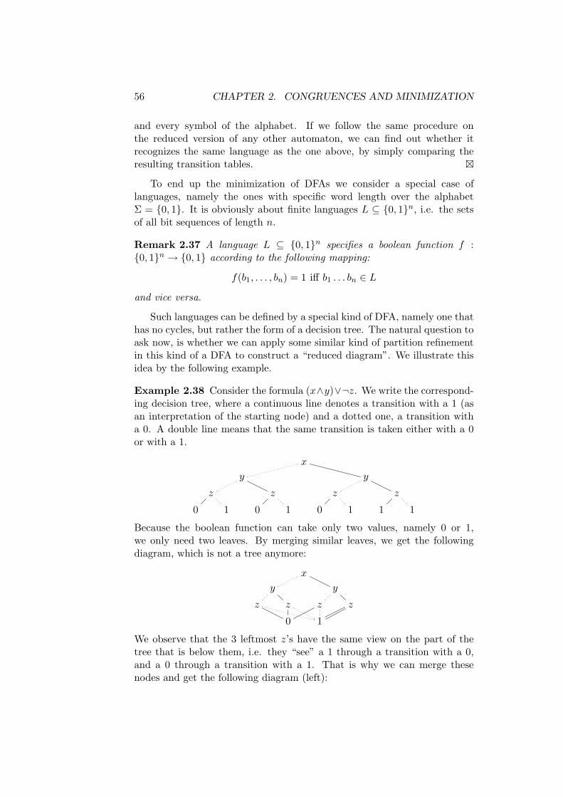
56 CHAPTER 2. CONGRUENCES AND MINIMIZATION
and every symbol of the alphabet. If we follow the same procedure onthe reduced version of any other automaton, we can find out whether itrecognizes the same language as the one above, by simply comparing theresulting transition tables. £
To end up the minimization of DFAs we consider a special case oflanguages, namely the ones with specific word length over the alphabetΣ = {0, 1}. It is obviously about finite languages L ⊆ {0, 1}n, i.e. the setsof all bit sequences of length n.
Remark 2.37 A language L ⊆ {0, 1}n specifies a boolean function f :{0, 1}n → {0, 1} according to the following mapping:
f(b1, . . . , bn) = 1 iff b1 . . . bn ∈ L
and vice versa.
Such languages can be defined by a special kind of DFA, namely one thathas no cycles, but rather the form of a decision tree. The natural question toask now, is whether we can apply some similar kind of partition refinementin this kind of a DFA to construct a “reduced diagram”. We illustrate thisidea by the following example.
Example 2.38 Consider the formula (x∧y)∨¬z. We write the correspond-ing decision tree, where a continuous line denotes a transition with a 1 (asan interpretation of the starting node) and a dotted one, a transition witha 0. A double line means that the same transition is taken either with a 0or with a 1.
x
y y
z z z z
0 1 0 1 0 1 1 1
Because the boolean function can take only two values, namely 0 or 1,we only need two leaves. By merging similar leaves, we get the followingdiagram, which is not a tree anymore:
x
y y
z z z z
0 1
We observe that the 3 leftmost z’s have the same view on the part of thetree that is below them, i.e. they “see” a 1 through a transition with a 0,and a 0 through a transition with a 1. That is why we can merge thesenodes and get the following diagram (left):

2.3. EQUIVALENCE AND REDUCTION OF NFAS 57
x
y y
z z
0 1
x
y
z
0 1
Finally, a node that leads to its (only) successor with both a 0 or a 1can be eliminated, because it does not affect the final result. This leads usto the final minimized diagram above (right). £
Formally the procedure can be described by the following reduction rules:
1. Merge two nodes p, q if they have isomorphic structures. (This corre-sponds to the relation p ∼A q for a DFA A)
2. In case there exist transitions p →b q and q →0 r, q →1 r, strike out qand introduce the transition p →b r.
Note that the second rule makes use of the fact that the nodes are labeledby the names of the variables. This way, striking out a node does not leadto processing the wrong bits. If we apply these reduction rules on a decisiontree, until no rules can be applied anymore, then the resulting diagram iscalled a “Reduced Ordered Binary Decision Diagram” (ROBDD).
Theorem 2.39 (Main Theorem on ROBDDs) The ROBDD for a booleanfunction does not depend on the order, in which the reduction rules are ap-plied: it is unambiguously defined up to isomorphism.
Corollary 2.40 The equivalence test for definitions of boolean functionscan be reduced on the isomorphism test of ROBDDs.
2.3 Equivalence and Reduction of NFAs
In this section we examine whether the problems that we efficiently solved inthe last section on DFAs are likewise efficiently solvable in the case of NFAs.The main motivation towards this goal is the fact that minimal NFAs canbe exponentially smaller than equivalent minimal DFAs with respect to thenumber of states.
Example 2.41 Consider the language Ln = the set of words over {a, b}having an a on the n-th position before the end. A minimal NFA canrecognize this language with n + 1 states by guessing when the n-th lastposition is being read and initiate a run of n transitions to the final state.On the contrary, a minimal DFA would always have to memorize the lastn letters that it has processed by having built in a path for each possiblecombination. This needs obviously 2n states. £

58 CHAPTER 2. CONGRUENCES AND MINIMIZATION
By this example we realize that the minimization of NFAs can save upa lot of space when modeling a system. Unfortunately, this does not comewithout a cost. In particular, in this section we deal with the followingissues:
• The PSPACE-hardness of the equivalence problem and the minimiza-tion problem for NFAs
• An efficient reduction of NFAs using the bisimulation equivalence be-tween states
• The Universal NFA and the search for a minimal NFA
We address only the decision problems of minimization, equivalence andnon-universality and show that even these are PSPACE-hard.NFA Minimization Problem
• Given: NFAs A,B over the same alphabet
• Question: Is B a minimal NFA equivalent to A?
NFA Equivalence Problem
• Given: NFAs A,B over the same alphabet
• Question: Are A and B equivalent?
NFA Non-Universality Problem
• Given: NFA A over the alphabet Σ.
• Question: Does L(A) 6= Σ∗ hold?
At the first glance this last problem looks very similar to our fairly known(and by the way very efficiently solvable) non-emptiness problem. However,we will see that there is a big difference between them.
Before we start, let us refresh our memory with some issues out of Com-plexity Theory. We know that a decision problem is P, NP or PSPACE if itcan be solved by a
• Turing Machine (TM) in polynomial time
• non-deterministic TM in polynomial time
• TM using at most polynomial space
respectively.
Remark 2.42 We code a decision problem by a language L as follows:L contains the word codings of those instances, for which the expected answeris “yes”.

2.3. EQUIVALENCE AND REDUCTION OF NFAS 59
Furthermore, we also know that P ⊆ NP ⊆ PSPACE and we stronglysuspect that the inclusions are proper.
Definition 2.43 A language L0 is PSPACE-complete, if
1. L0 belongs to PSPACE
2. Every language L ∈ PSPACE, say over the alphabet Σ, is reduciblein polynomial time to L0 (short: L ≤p L0), i.e. there exists functionF on Σ∗, such that it is computable in polynomial time and for allw ∈ Σ∗ w ∈ L iff F (w) ∈ L0 holds. In colloquial English, this meansthat a problem that has this property is at least as hard as any otherproblem in PSPACE.
L0 is PSPACE-hard, if the second condition holds.
Example 2.44 QBF, namely the evaluation problem for quantified booleanformulas is PSPACE-complete. £
Our aim is now to prove that all three decision problems mentionedabove are PSPACE-hard, i.e. they are not efficiently solvable like in thecase of DFAs. (It can be also shown that they belong to PSPACE, but weare not going to deal with that part of the proof.) For the case of the Non-Universality Problem of NFAs we have to prove that for every L in PSPACE“L ≤p NFA Non-Universality Problem” holds.
Lemma 2.45 For an arbitrary language L ⊆ Σ∗ that belongs to PSPACE,there exists a transformation F that is computable in polynomial time, suchthat F : Σ∗ → set of all NFAs over Σ′ with (∗) w ∈ L iff NFA F (w) doesnot accept all words over Σ′.
Proof: Let M be a Turing Machine that decides L using polynomial space.We define M by a tuple M = (Q,Σ, Γ, q0, δ, F ) with
• state set Q, initial state q0 ∈ Q, final state set F ⊆ Q
• working alphabet Γ, input alphabet Σ ⊆ Γ (with a distinguished blanksymbol à in Γ \ Σ)
• transition function δ : (Q \ F ) × Γ → Γ × {N, L, R} × Q
A transition δ(p, a) = (b, L/R/N, q) implies: “when being in state p andreading an a on the working cell, write there a b, move the head to the left/ move the head to the right / don’t move the head and go to state q”.Now assume the TM M decides L and is space-bounded by some polyno-mial p(n). The computational situation, in which M is, is described by itsconfiguration, which is defined by the word that is written on the left of the

60 CHAPTER 2. CONGRUENCES AND MINIMIZATION
working cell, the current state and the word that is written on the right ofthe working cell. So, a configuration of M has the form uqv.
Let w = a1 . . . an. An accepting computation M, w is a word over Γ ∪Q∪ {#} of the following form: u0q0v0 # u1q1v1 # . . . # usqsvs #, where
1. u0 = à . . . à and v0 = wà . . . Ã, and u0, v0 have been chosen in such away that throughout the whole computation M visits only the cellsoccupied by u0, v0, so |ui| + |vi| = p(n)
2. ui+1qi+1vi+1 is a successor configuration of uiqivi
3. usqsvs is a configuration with qs ∈ F
The purpose of the reduction is to find a transformation F computablein polynomial time with F : Σ∗ → set of all NFAs over the alphabet Σ′
having the property:
(∗) w ∈ L iff NFA F (w) does not accept all words in (Σ′)∗
We choose Σ′ = Γ∪Q∪{#} and we define the NFA F (w) in such a way thatit accepts exactly the words that are not an accepting M, w-computation.Then (∗) holds! To achieve this, the NFA F (w) has to check whether on theinput u one of the constraints 1. to 3. is indeed violated. In other words,the NFA has to verify that:
1. The input word does not begin with u0q0v0#,
2. OR there are two consecutive segments uiqivi#ui+1qi+1vi+1#, suchthat ui+1qi+1vi+1 is not a successor configuration of uiqivi
3. OR that the last configuration does not contain a final state.
The first condition can be tested with p(n)+2 states (because |u0v0| = p(n)).The second condition can be tested by guessing 3 consecutive cells, whoseupdate (after p(n) + 2 positions) is not correct. O(p(n) + 2) states sufficefor this test.
Explanation: Assume that the transition function of the Turing Machineimplies δ(p, b) = (a, L, q) and consider the following two consecutive config-urations (without the square brackets):
. . . [aab][apb] . . .# . . .︸ ︷︷ ︸
p(n)+2
[aab][qaa]
The automaton may compare the three consecutive cells in the first squarebrackets with the ones that are p(n) + 2 positions away. In the case thatnone of these cells is currently (or in the previous step) occupied by the

2.3. EQUIVALENCE AND REDUCTION OF NFAS 61
head of the Turing Machine, one cell would suffice for the comparison. Butin case one of the cells contains the state of the Turing Machine (like in thesecond square brackets) three cells are required. In the example above theNFA verifies that the Turing Machine changed from state p to q, movingthe head to the left (that is why the q is now written on the left of the athat was previously on the left of the p) and printing an a on the b. Inthis example the cells adhere to the transition function. In the general casethe Turing Machine has to guess such a pair of triples where this does nothold. It is now obvious that O(p(n) + 2) states suffice for this test, wherethe constant represents the space that is required to save a triple of cells likeit was mentioned above.
The last condition can be trivially tested by using a memory state toremember the information “no final state has been seen between the lasttwo #”. Consequently, from M and w we can construct the appropriateNFA F (w) as a union-NFA from the three automata mentioned above withp(n)+2, const·(p(n)+2) and 5 states respectively. Altogether, this NFA haspolynomially many states with respect to n = |w|, which also means thatthe transformation w 7→ F (w) is computable in polynomial time. Thus, wehave proven the following theorem:
Theorem 2.46 The NFA-Non-Universality Problem is PSPACE hard.
Now that we have extensively dealt with the non-universality problemon NFAs, let us compare it with a much more easily solvable problem thatlooks (at least at the first glance) similar to it, namely the non-emptinessproblem for NFAs. So, given an NFA A we compare the following questions:
1. L(A) = ∅? or the negation L(A) 6= ∅?
2. L(A) = Σ∗? or the negation L(A) 6= Σ∗?
The first question is about the existence of an appropriate w and the ex-istence of some corresponding accepting run on it, which, as we know, issolvable in linear time (by performing breadth-first or depth-first search).On the contrary, the second problem is about the existence of an acceptingrun for each possible w, or for the existence of such a w that all possi-ble runs on it are rejecting. Now we can see that there is a big differencein terms of logic between the two problems. The first one contains twoconsecutive existential quantification whereas the second is expressed by auniversal quantification followed by an existential one (or vice versa in thecase of the negation). The PSPACE hardness of the second problem reliesexactly on this alternation of the existential and the universal quantifier. Itis easy to see that the universality problem of an NFA A over Σ is a specialcase of the equivalence problem between A and the standard NFA A0 withjust one state that is also a final one (obviously accepting Σ∗). Likewise,
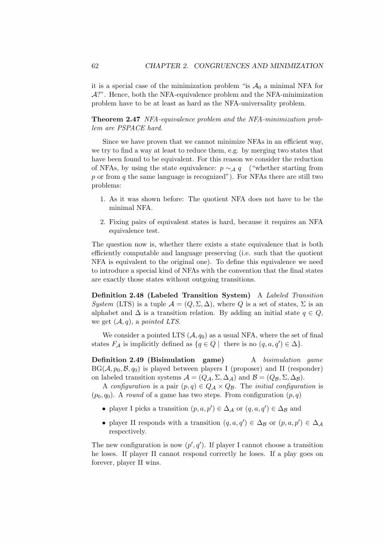
62 CHAPTER 2. CONGRUENCES AND MINIMIZATION
it is a special case of the minimization problem “is A0 a minimal NFA forA?”. Hence, both the NFA-equivalence problem and the NFA-minimizationproblem have to be at least as hard as the NFA-universality problem.
Theorem 2.47 NFA-equivalence problem and the NFA-minimization prob-lem are PSPACE hard.
Since we have proven that we cannot minimize NFAs in an efficient way,we try to find a way at least to reduce them, e.g. by merging two states thathave been found to be equivalent. For this reason we consider the reductionof NFAs, by using the state equivalence: p ∼A q (“whether starting fromp or from q the same language is recognized”). For NFAs there are still twoproblems:
1. As it was shown before: The quotient NFA does not have to be theminimal NFA.
2. Fixing pairs of equivalent states is hard, because it requires an NFAequivalence test.
The question now is, whether there exists a state equivalence that is bothefficiently computable and language preserving (i.e. such that the quotientNFA is equivalent to the original one). To define this equivalence we needto introduce a special kind of NFAs with the convention that the final statesare exactly those states without outgoing transitions.
Definition 2.48 (Labeled Transition System) A Labeled TransitionSystem (LTS) is a tuple A = (Q,Σ, ∆), where Q is a set of states, Σ is analphabet and ∆ is a transition relation. By adding an initial state q ∈ Q,we get (A, q), a pointed LTS.
We consider a pointed LTS (A, q0) as a usual NFA, where the set of finalstates FA is implicitly defined as {q ∈ Q | there is no (q, a, q′) ∈ ∆}.
Definition 2.49 (Bisimulation game) A bisimulation gameBG(A, p0,B, q0) is played between players I (proposer) and II (responder)on labeled transition systems A = (QA, Σ, ∆A) and B = (QB, Σ, ∆B).
A configuration is a pair (p, q) ∈ QA × QB. The initial configuration is(p0, q0). A round of a game has two steps. From configuration (p, q)
• player I picks a transition (p, a, p′) ∈ ∆A or (q, a, q′) ∈ ∆B and
• player II responds with a transition (q, a, q′) ∈ ∆B or (p, a, p′) ∈ ∆Arespectively.
The new configuration is now (p′, q′). If player I cannot choose a transitionhe loses. If player II cannot respond correctly he loses. If a play goes onforever, player II wins.

2.3. EQUIVALENCE AND REDUCTION OF NFAS 63
A strategy is a mapping σ : (QA × QB)+ → (QA ∪ QB) for player Iand similarly σ : (QA × QB)+(QA ∪ QB) → (QA ∪ QB) for player II. Awinning strategy for player II ensures that for every configuration (p, q) thatis reached while II plays according to this strategy, player I will not win theBG(A, p,B, q).
(A, p0) and (B, q0) are called bisimilar, (A, p0) ∼ (B, q0), if player II has awinning strategy in BG(A, p0,B, q0). In the special case that (A, p) ∼ (A, q)we call p and q ∼-equivalent (p ∼ q).
Proposition 2.50 (A, p0) ∼ (B, q0) ⇒ L(Ap0) = L(Bq0)
Proof: By assumption player II has a winning strategy in BG(A, p0,B, q0).We show L(Ap0) ⊆ L(Bq0). (The other direction is similar to this one.)
Assume w ∈ L(Ap0). We apply the winning strategy of player II to aplay where player I moves in A from p0 to FA by a path labeled w. Player IIrealizes a path in B starting from q0 and labeled with w. We have to checkthat the last state of this path is in FB. But this is clear, because otherwiseplayer II would lose in the next step. 2
The following example shows that the converse direction of proposition2.50 fails.
Example 2.51 Consider the following two NFAs:
•b
•
a
a
•
•c
• a •b
c
•
They accept the same language, but they are not bisimilar (both started ontheir leftmost state). £
Remark 2.52 Bisimulation equivalence is finer than language equivalence.This means that it results to a correct but not optimal reduction of an NFA.
To compute the bisimulation equivalence between two LTS we have tocheck for all states p, q whether (A, p) ∼ (B, q). Again, similar to the mini-mization algorithm for DFAs, we determine the pairs p, q where player I hasa winning strategy (showing non-equivalence).
Remark 2.53 1. If p ∈ FA and q 6∈ FB, or vice versa, player I winsafter his first move.

64 CHAPTER 2. CONGRUENCES AND MINIMIZATION
Input: LTS A = (QA,Σ,∆A), B = (QB,Σ,∆B)
1. Mark p, q ∈ QA × QB if p ∈ FA 6⇔ q ∈ FB
2. while some states have been marked in the last iteration do
3. Mark each pair p, q previously unmarked for whichthere is a (p, a, p′) ∈ ∆A such that for all (q, a, q′) ∈ ∆B
(p′, q′) is marked
4. Mark each pair p, q previously unmarked for whichthere is a (q, a, q′) ∈ ∆B such that for all (p, a, p′) ∈ ∆A
(p′, q′) is marked.
5. od
Output: All marked pairs.
Figure 2.3: Bisimulation Marking Algorithm
2. If player I can pick (p, a, p′) ∈ ∆A such that for all (q, a, q′) ∈ ∆B thatplayer II can choose, player I wins from (p′, q′), then from (p, q) playerI wins. Similarly, if player I can pick (q, a, q′) ∈ ∆B such that for all(p, a, p′) ∈ ∆A that player II can choose, player I wins from (p′, q′),then from (p, q) player I wins.
The Remark 2.53 motivates the marking algorithm for marking pairs(p, q) with (A, p) 6∼ (B, q) shown in Figure 2.3.
Example 2.54 We apply the marking algorithm to reduce the NFA shownbelow. According to our convention, the final states are 4 and 6. That is
1 2 3
4 5 6
a
a b
b
b
b
b
a
why before entering the loop, we mark all pairs, where exactly one of thosetwo states occurs. In the first loop we mark the pair (2, 1) because we canchoose to move from 2 with b, but we cannot move with the same letterfrom state 1. We also mark the pair (5, 2) because there exists a transitionwith b from 5 that leads to state 6 that is already marked with every statethat is reachable from 2 with the same transition (namely 3, since it is theonly state reachable with a b and (6, 3) is marked). Continuing like this, thealgorithm terminates leaving the pairs (5, 3) and (6, 4) unmarked.

2.3. EQUIVALENCE AND REDUCTION OF NFAS 65
1 2 3 4 52 1 X X X X3 1 1 X X X4 0 0 0 X X5 1 1 0 X6 0 0 0 0
X : It is not necessary to look at thisfield.
0 : This field was marked beforeentering the loop (final andnon-final states).
i : This field was marked in thei-th loop (i = 1, 2, . . .).
This means that we can merge these states in the reduced automaton.The resulting NFA is shown below and it happens to be also a minimal one.
1 2 3, 5
4, 6
a
ab
b
b
a
£
The algorithm terminates after ≤ |QA| · |QB| loops (all possible pairs ofstates). Every loop requires the consideration of each previously unmarkedpair (p, q) by checking the corresponding outgoing transitions, i.e. a compu-tational effort that is proportional to |QA| · |∆A| + |QB| · |∆B|. Altogether,if A,B have |QA| + |QB| = n states and |∆A| + |∆B| = m transitions, thenthe marking algorithm terminates in time O(n3m). Better algorithms areknown working in time O(n · log2(n)) (Page and Tarjan, 1987).
NFA A
NP-hard
PTIME
A− bisimulation quotient of A
gap in sizesmallest NFAs A0,A1, . . . ,Ak
There is a variant of BG(A, p,B, q) that results to wider equivalenceclasses, and is therefore often considered as more appropriate. It is calledthe alternating simulation and the main difference to bisimulation is thatthis time player I has to stay in the NFA that he chose in his first move,i.e. he cannot arbitrarily switch between the two NFAs. In this case thequotient NFA is again language equivalent and efficiently computable.
Example 2.55 For the following NFAs the alternating simulation holds,but not the bisimulation.

66 CHAPTER 2. CONGRUENCES AND MINIMIZATION
aa
ba
a
b
a
a
£
Finally, there is an alternative technique that leads not only to the reduced,but even to the minimal NFA. The idea relies on the fact that given an NFAwith n states, there are only finitely (of course exponentially) many NFAswith less than n states. The following procedure illustrates, how we canconstruct a (in most cases huge) NFA that contains all equivalent smallerNFAs and in which we can restrict our attention only to those NFAs whoreally have the possibility to be minimal ones. Given a regular language L,there is indeed a canonical NFA, in which we can search for the minimalone; it is constructed as follows:
1. Determine the minimal DFA AL (powerset construction andDFA-minimization)
2. In AL invert all transitions and switch all final states to initial onesand vice versa and thus obtain the NFA AL.
3. Once again apply the powerset construction to obtain D(AL) (deter-ministic).
4. Invert this DFA too and obtain D(AL).
5. The Universal-NFA C is constructed out of the state sets of the lastNFA.
The NFA D(AL) has states A1, . . . , Ak, each of them consisting of AL-states. The states of the Universal-NFA C are sets of the form {Ai1 , . . . , Aim},where Ai1 ∩ . . . ∩ Aim 6= ∅ must hold. For further details, please refer toO. Matz, A. Potthoff, “Computing Small Nondeterministic Automata”.
Theorem 2.56 The Universal-NFA of L contains each minimal NFA rec-ognizing L as an induced NFA for an appropriate subset of its states.
This confirms our initial claim, namely that the minimal NFA can be foundwithin the Universal-NFA.

2.4. THE SYNTACTIC MONOID 67
2.4 The Syntactic Monoid
In this section we introduce a structure that characterizes a regular languagebut also contains a neutral element and enables us to perform binary opera-tions just like in the case of natural numbers. The reason why we find sucha structure very useful to describe a language, is that the set of all wordsfollows the same concept (neutral element, binary operations) but automatadon’t. In other words we shall see that using this structure we can directlyidentify characteristics of a language that cannot be directly handled by au-tomata, like for example whether a language is star-free (i.e. FO-definableor LTL-definable)
Exactly as the minimal DFA is a canonical acceptor for a regular lan-guage L, we define a further canonical acceptor M(L), the “syntactic monoid”for L, with the same signature as for all words over Σ, namely (Σ∗, ·, ε).
There is a close relation between the monoid structure and the transitionstructure of the minimal DFA AL. This relation is presented in the following.First, we refine the Nerode congruence by making it symmetric:
Definition 2.57 For a language L ⊆ Σ∗ we define: u ≈L v if ∀x, y ∈ Σ∗ :xuy ∈ L ⇔ xvy ∈ L.
Remark 2.58 ≈L is a right congruence with respect to concatenation, i.e.≈L is an equivalence relation and u ≈L v, u′ ≈L v′ ⇒ uu′ ≈L vv′. If u ≈L vand u′ ≈L v′, then xuu′y ∈ L iff xvv′y ∈ L for all words x and y.
Remark 2.59 u ≈L v implies u ∼L v (take x = ε). The converse does nothold in general.
Example 2.60 Consider the language L = bba∗. a ∼L ba, because for allw ∈ Σ∗: aw /∈ L and baw /∈ L. But a 6≈L ba, because b · a · ε /∈ L, andb · ba · ε ∈ L. £
Notation:
• The ≈L-class of u ∈ Σ∗ is denoted by 〈u〉L.
• Let Σ∗/≈Lbe the set of all ≈L-classes.
A multiplication (concatenation) between ≈L-classes is defined by rep-resentatives: 〈u〉L · 〈v〉L := 〈uv〉L. The product is well-defined because ≈L
is a right congruence.
Remark 2.61 (Σ∗, ·, ε) is a monoid (i.e. · is associative, and ε is the neu-tral element).

68 CHAPTER 2. CONGRUENCES AND MINIMIZATION
The structure M(L) := (Σ∗/≈L, ·, 〈ε〉) is also a monoid, namely the syn-
tactic monoid of L. But how can we construct the correct monoid for alanguage? We do this by applying specific transformations on the automaton(we take the canonical one) that recognizes this language.
Let A = (Q,Σ, q0, δ, F ) be a DFA. Every word w ∈ Σ∗ induces a statetransformation wA : Q → Q that is defined by wA(q) := δ(q, w). Note thatεA = idQ (identity function). The composition goes as follows: uA ◦ vA isthe function (uv)A: uA ◦ vA(q) = vA(uA(q)).
Remark 2.62 The structure T (A) = ({uA | u ∈ Σ∗}, ◦, idQ) is a monoid,namely the transition monoid of A.
Note that over Q, there are at most |Q||Q| many functions. This meansthat the transition monoid of a DFA is finite. If Q = {0, . . . , n}, then werepresent the state transformation uA by the sequence uA(0), . . . , uA(n) ofvalues on the states of the DFA.
Example 2.63 Consider the following automaton and the transformationsbeside.
0 1
2
a
aa
b
b
b
εA: (0 1 2)aA: (1 2 0)aaA: (2 0 1)
£
One can easily see that there are no other (different) transformations on thisDFA, e.g. bA = εA or aabaaA = aA. But of course this is no proof that wehave indeed found all possible transformations. There is a formal methodto determine all functions uA and it goes as follows:
1. Go through all words u in canonical order, until no new functionsoccur.
2. Draw an a-labeled arrow from uA to (ua)A
Example 2.64 Let L1 := {w ∈ Σ∗ | |w|a ≡ 0 (mod 3) }. The DFA AL1 isshown below:

2.4. THE SYNTACTIC MONOID 69
0 1
2
a
aa
b
b
b
012ε
ab
120a
a
b
201aa
a
b
Having determined the functions from the previous example, we draw thetransition monoid (on the right). £
Example 2.65 Consider the language L2 := { aw ∈ Σ∗ | |w| ≡ 0 (mod 2) }recognized by the following automaton AL2 :
0 1
23
a
b a, ba, b
a, b
0123ε
a
b
1213a
a,b2123aa
a,b
3213b
a,b3123ba
a,b
The corresponding transition monoid T (AL2) is drawn on the right. £
Example 2.66 L3 := (ab)∗ is recognized by the following automaton AL3 :
0 1
2
ab
a
b
a, b
122a
b
a
022ab
ab
012ε
a
b
222aa
a,b
202b
a
b
212ba
a
b
The corresponding transition monoid T (AL3) is drawn on the right. £
Now we can proceed to constructing the syntactic monoid. For thispurpose we prove the following theorem.
Theorem 2.67 Let L be regular and AL the minimal automaton recognizingL. The syntactic monoid M(L) is isomorphic to the transition monoid ofAL, short: M(L) ∼= T (AL).

70 CHAPTER 2. CONGRUENCES AND MINIMIZATION
Hence, by constructing the transition monoid (by using the previously il-lustrated method) and by applying the last theorem, we obtain the syntacticmonoid.
Proof: Define f : M(L) → T (AL) by f(〈u〉) := uAL . f is the appropriateisomorphism. f is well-defined and injective because
〈u〉 = 〈v〉 iff uAL = vAL .
Verification: 〈u〉 = 〈v〉
iff ∀x, y : xuy ∈ L ⇐⇒ xvy ∈ L
iff ∀x : [xu] = [xv] (by definition)
iff ∀x : uAL([x]) = vAL([x])(Note that [x] is a state of AL and uAL([x]) = [xu])
iff uAL = vAL
f is surjective, because
uAL = f(〈u〉) for all uAL ∈ T (AL)
Finally, f is a homomorphism, because
f(〈u〉 · 〈v〉) = f(〈uv〉) = (uv)AL = uAL ◦ vAL = f(〈u〉) ◦ f(〈v〉)
2
Now we can use these results to identify the class, in which a languagebelongs. For example, in the previous chapter we have shown that the star-free languages are non-counting. In the following we show that it can beidentified, whether a language is non-counting, by the property “group-free”of the syntactic monoid. Furthermore, we show that for regular languages,the properties non-counting and star-free coincide.
Definition 2.68 An element m of a monoid M is called idempotent, ifm · m = m.
Every subset of M that forms a group through multiplication ·, hasexactly one idempotent element. This is the neutral element of the group.We call a monoid M group-free if the only occurring subsets that form groupsare the trivial ones {m} with an idempotent m.
Example 2.69 We look at the monoid of a previous example.

2.4. THE SYNTACTIC MONOID 71
012ε
ab
120a
a
b
201aa
a
b
ε a aa
ε ε a aaa a aa εaa aa ε a
0 1 2
0 0 1 21 1 2 02 2 0 1
Obviously the whole monoid represents a non-trivial group, since it is count-ing modulo-3. The two multiplication and addition tables show the corre-spondence between this monoid and the group (Z3, +) respectively. £
Example 2.70 Consider the following two monoids.
0123ε
a
b
1213a
a,b2123aa
a,b
3213b
a,b3123ba
a,b
122a
a
b022ab
a
b
012ε
a
b
222aa
a,b
122b
b
a022ba
b
a
The left one has two groups, each one of the type Z2, while the right onedoes not have any non-trivial groups, i.e. it is group-free. £
Theorem 2.71 (Schutzenberger 1965) Let L be regular. L is star-freeif and only if M(L) is group-free.
According to this theorem, one can algorithmically decide, whether a givenregular language is star-free.
Example 2.72 According to the previous examples:
1. L1 := {w ∈ Σ∗ | |w|a ≡ 0 (mod 3) } is not star-free.
2. L2 := { aw ∈ Σ∗ | |w| ≡ 0 (mod 2) } is not star-free.
3. L3 := (ab)∗ is star-free.
£
Theorem 2.71 allows even the generation of a star-free expression out ofa given group-free monoid. This is implemented in the AMoRE system.
We can also determine whether a monoid M(L) is group-free by directlyanalyzing the corresponding minimal DFA AL. The required property isgiven in the following definition.

72 CHAPTER 2. CONGRUENCES AND MINIMIZATION
Definition 2.73 A DFA A = (Q,Σ, q0, δ, F ) allows permutations, in casethere exist a subset Q0 ⊆ Q and a word w ∈ Σ+, such that wA|Q0 rep-resents a non-trivial permutation on Q0. In the opposite case A is calledpermutation-free.
Example 2.74 We examine the minimal deterministic automata recogniz-ing the three languages of the previous examples.
AL1 :
0 1
2
a
aa
b
b
b
This DFA allows permutations. Take Q0 = {0, 1, 2} and w = a. ThenaAL1 |{0,1,2} represents a non-trivial permutation on {0, 1, 2} (0 1 2 7→ 1 2 0).
AL2 :
0 1
23
a
b a, ba, b
a, b
This DFA allows permutations. Take Q0 = {1, 2} and w = a. ThenaAL2 |{1,2} represents a non-trivial permutation on {1, 2} (1 2 7→ 2 1).
AL3 :
0 1
2
ab
a
b
a, b
This DFA is permutation-free. £
Finally, we gather all the previous properties of a regular language inthe following theorem.
Theorem 2.75 For a regular language L the following conditions are equiv-alent:
(a) L is non-counting.

2.4. THE SYNTACTIC MONOID 73
(b) The minimal DFA AL is permutation-free.
(c) The syntactic monoid M(L) is group-free.
(d) L is star-free.
According to the theorem of Schutzenberger (c) ⇔ (d). In the following weshow
• not (c) ⇒ not (b),
• not (b) ⇒ not (a),
• not (a) ⇒ not (c).
Proof (from group to permutation): Assume M(L) is not group-free,say having a group G. Choose a g ∈ G other than the neutral elementof G and consider the cyclic group {g, g2, . . . , gk} with gk as a neutral el-ement. g = 〈u〉 corresponds via the isomorphism M(L) ∼= T (AL) to thetransformation uAL . Then gi = 〈ui〉, and the following holds:
1. (uk)AL = (u2k)AL
2. (uk)AL 6= (uk+1)AL
Now choose a q, such that δ(q, uk) 6= δ(q, uk+1). Set Q0 = {δ(q, uk),δ(q, uk+1), . . . , δ(q, u2k−1)}. Then uAL is a permutation on Q0. 2
Proof (from permutation to modulo-counting): Let the transforma-tion vAL be a permutation π on Q0. Choose a q ∈ Q0 and obtain the ele-ments q, π(q), π2(q), . . . , πm(q) = q. Then δ(q, vkm) = q, δ(q, vkm+1) = q′ 6=q. Choose u, w such that δ(q0, u) = q, and not δ(q, w) ∈ F ⇔ δ(q′, w) ∈ F .Now we have to show that for any arbitrarily large n:
∃u, v, w: not uvnw ∈ L ⇔ uvn+1w ∈ L
Take n = km where k is arbitrary. Then it does not hold that
δ(q0, uvkmw) ∈ F ⇔ δ(q0, uvkm+1w) ∈ F
2
Proof (from modulo-counting to group): Note that in every finitemonoid each element m has a power mk that is idempotent. Now set K =the smallest common multiple of these k-values. For every element m of amonoid mK = m2K (∗). By hypothesis there are arbitrarily large n’s (also> K), such that for appropriate u, v, w:
uvnw ∈ L but uvn+1w 6∈ L
For such an n then 〈vn〉 6= 〈vn+1〉. Because of (∗), 〈vK〉 = 〈v2K〉. Then〈vK〉 6= 〈vK+1〉 must hold. Now 〈vK+1〉 forms a group in M(L). 2

74 CHAPTER 2. CONGRUENCES AND MINIMIZATION
2.5 Exercises
Exercise 2.1 Find a family (Ln)n>0 of languages over {a, b}, such that
• Ln is recognized by a DFA with O(n) states, and
• every DFA that recognizes LRn has at least 2n many states.
Hint: The first automaton of Example 2.14 points to the right direction.(LR
n = {bn · · · b1 | b1 · · · bn ∈ L} is the language of the flipped words.)
Exercise 2.2 ∗ Consider the following algorithm that is applied on a DFAA (over Σ = {a, b}):
1. Invert A, i.e. turn the A-transitions to the opposite direction andswitch the initial states with the final ones. Obtain AR. (Note thatthe automaton may have several initial states.)
2. Apply the powerset construction (construct only the reachable states).Obtain D(AR). (The initial state of this automaton is the set of initialstates of the NFA.)
3. Invert D(AR), obtain (D(AR))R.
4. Apply the powerset construction as in (2), obtain D((D(AR))R).
Show that the resulting automaton is the minimal automaton for A.
Exercise 2.3 Consider the language L = b(a + b)∗aa over the alphabet{a, b}.(a) Give representatives for the five ∼L-classes.
(b) Verify that the representatives are pairwise not language equivalent, i.e.for any pair u, v, u 6∼L v holds (construct a table, where for each pair aseparating word w is entered).
(c) Using (a) give the minimal automaton AL for L.
Exercise 2.4 (a) Apply the minimization algorithm (page 54) in order tominimize the following DFA (describe the steps as in Example 2.34):
1a
b
2
a
b
3b
a
4b
a
5a
b
6a,b
7a
b
8
a
b

2.5. EXERCISES 75
(b) Construct the bisimulation quotient A of the following NFA A:
8
b
a,b
a
5
b
a
a,b4
a1
7
a
b
a
6
b
a
a,b
3
aa,b
b2
a
a,b
b
Exercise 2.5 Consider the DFA A without final states as given by thefollowing transition graph:
1
a
b2
a
b
3
a
b
Choose final states such that A is minimal, or show that this is impossible.
Exercise 2.6 ∗ Show that there exists a family of regular languages lan-guages (Ln)n>0 such that Ln is recognized by n different (not isomorphic)minimal NFAs.Hint: The editors do not know the solution yet.
Exercise 2.7 (a) determine the transition monoid of the following automa-ton according to the method presented in the lecture:
0
b
a1
b
a
2
a,b
Mark with a circle the idempotent elements.
(b) Determine the transition monoid (with 13 elements) of the followingautomaton:
0
b
a1
b
a
2
b
a
3
ab
Give a non-trivial group.

76 CHAPTER 2. CONGRUENCES AND MINIMIZATION
Exercise 2.8 ∗ Give a family of DFAs An = (Qn, Σ, qn0 , δn, Fn), n > 0, with
|Qn| = n over the alphabet Σ = {a, b, c}, such that the transition monoid ofAn has exactly nn elements. Hence, every mapping f : Qn → Qn has to beimplemented by a word in Σ∗.

Chapter 3
Tree Automata
In the last two chapters we dealt with two fundamental issues in the world offinite automata, namely establishing a connection to logical (or “logic-like”)expressions and discovering algebraic ideas and methods to solve typicalproblems on finite automata. In this chapter we are going to generalize themodel of a finite automaton itself, and use it for processing generalized inputs(i.e. not only finite words). This can be done in two different dimensions.One is to lift the constraint of finiteness and consider infinite inputs suchas the run of a non-terminating procedure. In this case we are not anymoreinterested in reaching some final state but rather in ensuring stability, e.g.by passing again and again through a certain state. The other is to consider(finite) inputs that are branching rather than being linearly ordered (i.e.letters follow one another).
The first dimension goes beyond the scope of this course and is the coreof the next semester’s course about automata over infinite objects. Thesecond dimension leads to the tree automata and tree languages, which areour main subject in this chapter.
Our primary motivation relies on the fact that trees model structuredobjects, which happen to be very frequent in computer science. Even thefinite words we were dealing with in the previous chapters are a special casein this category; they represent linear trees (only one successor). The fun-damental questions we are going to answer are accordingly a generalizationof the ones we considered in the last two chapters, i.e.:
• Which techniques can we borrow from the area of finite words?
• How can we construct automata that describe the properties of trees?
• How can we define equivalent formalisms like regular expressions andlogical formulas?
• Are there efficient algorithms for the fundamental problems (non-emptiness, equivalence and minimization of automata)?
77
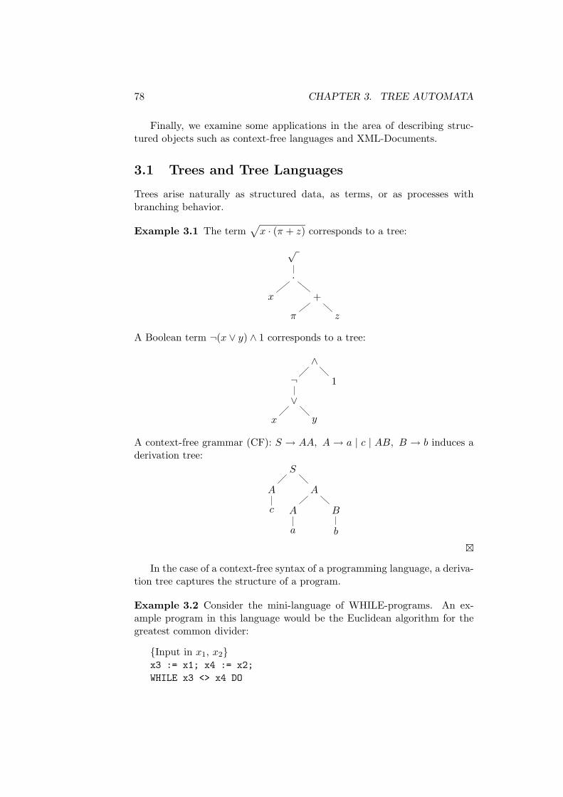
78 CHAPTER 3. TREE AUTOMATA
Finally, we examine some applications in the area of describing struc-tured objects such as context-free languages and XML-Documents.
3.1 Trees and Tree Languages
Trees arise naturally as structured data, as terms, or as processes withbranching behavior.
Example 3.1 The term√
x · (π + z) corresponds to a tree:
√
·x +
π z
A Boolean term ¬(x ∨ y) ∧ 1 corresponds to a tree:
∧¬ 1
∨x y
A context-free grammar (CF): S → AA, A → a | c | AB, B → b induces aderivation tree:
S
A A
c A B
a b
£
In the case of a context-free syntax of a programming language, a deriva-tion tree captures the structure of a program.
Example 3.2 Consider the mini-language of WHILE-programs. An ex-ample program in this language would be the Euclidean algorithm for thegreatest common divider:
{Input in x1, x2}x3 := x1; x4 := x2;
WHILE x3 <> x4 DO

3.1. TREES AND TREE LANGUAGES 79
IF x3 < x4 THEN x4 := x4 - x3 ELSE x3:= x3 - x4 END
END
{the value of x3 is gcd(x1, x2)}
A formal definition of the WHILE-programs includes:
• a terminal alphabet: Σkeyboard
• non-terminal symbols:S for 〈program〉W for 〈assignmentofvalue〉V for 〈variable〉D for 〈decimal number〉Z for 〈positive digit〉F for 〈sequence of decimal digits〉B for 〈condition〉O for 〈comparison operator〉E for 〈arithmetic expression〉
• a grammarS → W | S; S | IF B THEN S ELSE S END |
WHILE B DO S END
W → V := EV → XDD → 0 | Z | ZFF → 0 | Z | 0F | ZFZ → 1 | 2 | 3 |4 | 5 | 6 | 7 | 8 | 9E → D | V | (E + E) | (E − E) | (E · E)B → EOEO → = | < | > | <> | =< | =>
According to this definition a possible syntax tree of the gcd-program looksas follows:
S
S ; S
W S ; S
W WHILE B DO S END
. . . IF B THEN S ELSE S END
. . . . . . . . .
£
We know that it is very important to point out the hierarchical structureof a program even in its normal text representation. That is why program-mers use indents to show how expressions are nested in each other. A similar

80 CHAPTER 3. TREE AUTOMATA
way to represent the structure of a derivation tree in normal text form is theuse of special bracketing. For every non-terminal symbol X the brackets (X
and )X are introduced. Then, the derivation tree t for w is coded by theword wt that is produced by inserting bracketing symbols into w.
Example 3.3 The derivation tree on the left can be coded by the word onthe right.
S
A A
A B a
c b
(S (A (A c )A (B b )B )A (A a )A )S
£
XML-documents are also coding trees in normal text form. Here, thebracketing notation is slightly modified: 〈X〉 is used for (X and 〈/X〉 isused for )X .
Example 3.4 Consider the following XML-document:
<ProfileOfStudies>
<faculty> Computer Science </faculty>
<semester> 3 </semester>
<courses>
<title> PROGRAMMING </title>
<title> COMPUTER STRUCTURES </title>
<title> DATA STRUCTURES </title>
</courses>
</ProfileOfStudies>
The main difference between the previous examples and XML-documents isthat in the latter the branching degree is generally unlimited. For examplethere is no restriction on the number of titles that the “courses”-bag maycontain. This case is considered in further detail later. £
Definition 3.5 A ranked alphabet is a non-empty finite set Σ of symbols,where every symbol a is assigned a finite set rk(a) ⊆ N (the set of all ranksor arities of a).
Σi := { a ∈ Σ | i ∈ rk(a) }
Σ = Σ0 ∪ · · · ∪ Σm (where m = max{rk(a) | a ∈ Σ})Note that the Σi need not be disjoint.

3.1. TREES AND TREE LANGUAGES 81
Example 3.6 The ranked alphabet for the term√
x · (π + z) from Example3.1 is Σ = {√ , +, ·, x, π, z} with Σ2 = {+, ·}, Σ1 = {√ } and Σ0 = {x, π, z}.
£
Example 3.7 The ranked alphabet for the term ¬(x∨y)∧1 from Example3.1 is Σ = {0, 1,¬,∧,∨} with Σ0 = {0, 1}, Σ1 = {¬}, Σ2 = {∧,∨}. £
Example 3.8 The ranked alphabet for the context-free grammar from Ex-ample 3.1 is Σ = {a, b, c, A, B, S} with Σ0 = {a, b, c}, Σ1 = {A, B}, Σ2 ={S, A}. £
We first define trees in a term-like fashion.
Definition 3.9 Let Σ = Σ0 ∪ . . .∪Σn be a ranked alphabet. The set TΣ oftrees (or terms) over Σ is defined inductively by:
• Each symbol a ∈ Σ0 is a tree a ∈ TΣ.
• For f ∈ Σk and t1 . . . tk ∈ TΣ, f(t1 . . . tk) is a tree in TΣ depicted by
f
t1 t2 . . . tk−1 tk
A set T ⊆ TΣ is called a tree-language.
Remark 3.10 This definition of trees allows
• inductive definitions of functions on the set of Σ-trees
• proofs by induction over the construction of Σ-trees.
Example 3.11 Inductive definitions:
1. The frontier word yield(t) of a tree t (the labelling of the leaves of tread from left to right) is inductively defined byyield(a) = a for a ∈ Σ0,yield(a(t1, . . . , ti)) = yield(t1) · · · yield(ti) for a ∈ Σi (i > 0).
2. Semantics of WHILE-programsLet WHILEn be the set of WHILE-programs with the variables x1, . . . , xn.Each such program computes a partial function f : Nn− → Nn. LetFn be the set of these functions. Then, the semantics of a programis a function σ : WHILEn → Fn that is defined inductively over thestructure of the program.
£
Example 3.12 An inductive proof for the arithmetical terms over {0, 1, +, ·}:

82 CHAPTER 3. TREE AUTOMATA
Hypothesis: The modulo-3 value of a term t with at most one 1, is either0 or 1.
Inductive proof:
1. Induction start:Verify the hypothesis for the terms 0 and 1.
2. Induction step:Assume the hypothesis is fulfilled for t1, t2. Show that the hypothesisholds for (t1 + t2) and (t1 · t2) (by simply distinguishing the possiblecases).
£
An alternative, but equivalent, definition of trees distinguishes the tree-domain, which is the set of underlying nodes, from their values under anevaluation function.
Example 3.13 Below the tree associated to the term ¬(x ∨ y) ∧ 1 and itsunderlying domain is shown. The evaluation function val satisfies val(ε) =∧; val(1) = ¬, . . .
∧¬ 1
∨x y
ε
1 2
11
111 112
£
Definition 3.14 Let Σ = Σ0 ∪ . . . ∪ Σn be a ranked alphabet. A Σ-valued tree is a tuple t = (domt, valt) where domt is a prefix closed subsetof {1, . . . n}∗ satisfying ui ∈ domt ⇒ uj ∈ domt for every j < i, andvalt : domt → Σ maps a node u with k successors to a symbol in Σk.
3.2 Tree Automata
3.2.1 Deterministic Tree Automata
Definition 3.15 A deterministic tree automaton (DTA) is a tuple A =(Q,Σ, δ, F ) where
• Q is a finite set of states,
• Σ is a ranked alphabet,

3.2. TREE AUTOMATA 83
• F ⊆ Q is a set of final states, and
• δ :⋃
i≥0(Qi × Σi) → Q is a transition function.
By convention Q0 × Σ0 := Σ0. The evaluation function δ∗ : TΣ → Qis defined inductively by δ∗(a) = δ(a) for a ∈ Σ0, and δ∗(f(t1 . . . ti)) :=δ(δ∗(t1), . . . , δ∗(ti), f) for f ∈ Σi and t1, . . . , ti ∈ TΣ.
A DTA A accepts a tree t ∈ TΣ if δ∗(t) ∈ F . The tree-language recognizedby A is T (A) = {t ∈ TΣ | A accepts t}.
Example 3.16 We define a tree automaton accepting all true Boolean ex-pressions over Σ = {∧,∨,¬, 0, 1}. Let Q = {q0, q1} be the state set, F = {q1}be the set of final states, and δ be defined by
δ(0) = q0
δ(1) = q1
δ(qi,¬) = q|i−1|δ(qi, qj ,∧) = qmin(i,j)
δ(qi, qj ,∨) = qmax(i,j)
£
Definition 3.17 T is called DTA-recognizable or regular, if there exists aDTA A with T = T (A).
Example 3.18 The set of the true logical expressions (the ones that canbe evaluated to 1) is regular. £
Example 3.19 (on arithmetic expressions) Let Σ = Σ0 ∪ Σ2 with Σ0 ={0, 1}, Σ2 = {+, ·}. We construct a tree automaton that recognizes the treelanguage T = {t ∈ TΣ | value of t = 0 (mod 3)} . A tree that belongs tothis language is shown in the picture below. On the same picture, the runof the automaton, which we intend to construct, is shown; namely we use 3states to distinguish the 3 different cases in modulo-3 counting.
+q0
·q2 +q1
1q1 +q2 0q0 1q1
1q1 1q1
Formally: We use a state set Q = {q0, q1, q2}, where qi means that “themodulo-3 remainder of the evaluated term is i”. Obviously, q0 is the only fi-nal state. The transition function is defined explicitly for each possible value

84 CHAPTER 3. TREE AUTOMATA
of its arguments, using a parametric formulation for matters of compactness:
δ(0) = q0, δ(1) = q1
δ(qi, qj , +) = qi+j mod 3, δ(qi, qj , ·) = qij mod 3
£
In the following we consider 3 further examples of languages, in order toget more familiar with constructing DTAs.
Example 3.20 Let Σ = Σ0 ∪ Σ1 ∪ Σ2 with Σ0 = {0, 1}, Σ1 = {g} ,andΣ2 = {f}. We define tree automata for the languages
T1 = {t ∈ TΣ | there is an odd number of f ’s in t}T2 = {t ∈ TΣ | there are at least two f ’s in t}T3 = {t ∈ TΣ | on the frontier of t there is no 1 before a 0}
For T1 let Q = {q0, q1} and F = {q1}. q0 signals an even number of f ’sand q1 an odd number of f ’s in the subtree below the current node. Thisinduces the following transition function:
δ(0) = δ(1) = q0
δ(qi, g) = qi
δ(qi, qj , f) = q(i+j+1) mod 2
For T2 let Q = {q0, q1, q2} (signaling respectively no, one and at least twooccurrences of an f in the subtree below the current node) and F = {q2}.This induces the following transition function:
δ(0) = δ(1) = q0
δ(qi, g) = qi
δ(qi, qj , f) = qmin(i+j+1,2)
For T3 let Q = {q0, q1, q01, q10} and F = {q0, q1, q01}. A node of the treeis labeled with state q01 if all 0’s are before the first 1 in the frontier wordof the subtree below this node. q10 signals that there is a 1 somewhere leftof a 0 on the frontier, and q0, q1 signal that only 0’s, respectively 1’s, appearon the frontier of the corresponding subtrees. The meaning of the statesis implemented in the following transition function: δ(0) = q0, δ(1) = q1,δ(q, g) = q for all q ∈ Q,
δ(q0, q0, f) = q0 δ(q01, q0, f) = q10
δ(q1, q1, f) = q1 δ(q01, q1, f) = q01
δ(q0, q1, f) = q01 δ(q0, q01, f) = q01
δ(q1, q0, f) = q10 δ(q1, q01, f) = q10,
and δ(p, q, f) = q10 for all other combinations of states p, q ∈ Q. £

3.2. TREE AUTOMATA 85
Tree languages can also be defined by the rules of context-free grammars.How do these languages relate to the regular languages we illustrated so far?
Definition 3.21 If G = (N, T, P, S) is a context-free grammar, then letT (G) be the set of all derivation trees generated by G (with frontier wordsconsisting of T -symbols).
For this definition we assume that ε is not used in the grammar.
Example 3.22 The derivation tree on the right belongs to the language de-fined by the grammar on the left.
S → AAA → c | a | ABB → b
S
A A
c A B
a b
£
The following theorem shows that this kind of tree languages forms aproper subset of the regular ones.
Theorem 3.23 a) If G is a context-free grammar, then T (G) is regular.
b) Not every regular tree language can be represented as a language T (G)for a context-free grammar G.
Proof: (part a) Given a grammar G = (N, T, P, S) we construct a DTAwith state set N ∪ T ∪ {∗} and final state S. The tree automaton shouldbe able to copy the tree symbols into its states, as long as the tree is builtup (in a bottom-up fashion) according to the rules of G. Hence, the inputalphabet consists of Σ0 = T and Σi = {X ∈ N | there exists a rule X →α with |α| = i} (for i > 0). The transition function is defined as follows:
δ(a) = a for a ∈ Σ0
δ(σ1, . . . , σi, X) = X for X → σ1 . . . σi ∈ P for i > 0, X ∈ Σi
δ(σ1, . . . , σi, X) = ∗ otherwise (“error′′ − state)
δ(σ1, . . . , σi, ∗) = ∗
2
Proof: [part b] It suffices to show that there exists a tree language thatcannot be represented as a language of derivation trees. For this reason weconsider the set T containing all trees with the following property:
(∗) On every path there are at most two A’s and there exists at least onepath with two A’s.

86 CHAPTER 3. TREE AUTOMATA
Looking at this property, on the one hand we observe that T is a regularlanguage because (∗) is a conjunction of two properties that can be easilyrecognized by a DTA. On the other hand we also observe that in case asymbol A occurs twice in a path of a derivation tree t (as a result of asequence of grammar rules), then it is possible to produce trees with anarbitrary number of A’s on the same path (using the same sequence of rulesagain and again). Consequently, T is recognizable by a DTA but cannot beof the form T (G) for a grammar G. 2
Finally, we illustrate an example of a language that belongs to a higherclass in the sense that it is not recognizable by a DTA.
Example 3.24 Let Σ = Σ0 ∪ Σ2 with Σ0 = {b}, Σ2 = {a}. We show thatthe language T := { a(t, t) | t ∈ TΣ } is not recognizable. By a(t, t) we meanwhat is shown in the picture below, where t is a (sub)tree.
a
t t
When reading the root of a tree, the only information a DTA can get fromthe two subtrees below, is the states it reaches at the top of each subtree.Hence, the idea to prove this assumption (as well as other similar ones) isto show that the finitely many states of the DTA do not suffice to comparethe infinitely many different subtrees.
Proof: Towards a contradiction, we assume that the DTA A = (Q,Σ, δ, F )recognizes T . Since we do not have a restriction on the length of thetree, there are obviously infinitely many trees over Σ. But because Q isfinite, there exist two different trees t, t′ with δ∗(t) = δ∗(t′) and hence alsoδ∗(a(t, t)) = δ∗(a(t, t′)) (at this point the automaton cannot distinguish be-tween t and t′ anymore, since both lead it to the same state). Now, sinceδ∗(a(t, t)) ∈ F also δ∗(a(t, t′)) ∈ F , which means that a(t, t′) ∈ T . Contra-diction. £
In case we want to generate a similar repetition of states, this time onlyon the same path, we use another method that relies on the pumping lemma.To achieve this we first have to formally describe how we can concatenatetrees to get longer and longer paths. In the case of finite words no specialdefinition was required, because it is obvious that we append a word at the(only) end of another one. In the case of finite trees we do not have onespecific end, but instead a number of leaves; hence we have to always declareat which one of them we append a new tree when concatenating.
Definition 3.25 Let Σ be a ranked alphabet and c a new symbol of rank0. A special tree over Σ is a tree over Σ ∪ {c}, where c occurs exactly once(as a leaf). We call SΣ the set of all special trees over Σ. For t ∈ TΣ or
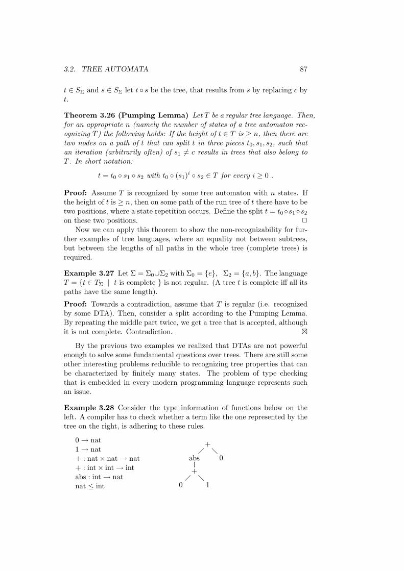
3.2. TREE AUTOMATA 87
t ∈ SΣ and s ∈ SΣ let t ◦ s be the tree, that results from s by replacing c byt.
Theorem 3.26 (Pumping Lemma) Let T be a regular tree language. Then,for an appropriate n (namely the number of states of a tree automaton rec-ognizing T ) the following holds: If the height of t ∈ T is ≥ n, then there aretwo nodes on a path of t that can split t in three pieces t0, s1, s2, such thatan iteration (arbitrarily often) of s1 6= c results in trees that also belong toT . In short notation:
t = t0 ◦ s1 ◦ s2 with t0 ◦ (s1)i ◦ s2 ∈ T for every i ≥ 0 .
Proof: Assume T is recognized by some tree automaton with n states. Ifthe height of t is ≥ n, then on some path of the run tree of t there have to betwo positions, where a state repetition occurs. Define the split t = t0 ◦s1 ◦s2
on these two positions. 2
Now we can apply this theorem to show the non-recognizability for fur-ther examples of tree languages, where an equality not between subtrees,but between the lengths of all paths in the whole tree (complete trees) isrequired.
Example 3.27 Let Σ = Σ0∪Σ2 with Σ0 = {e}, Σ2 = {a, b}. The languageT = {t ∈ TΣ | t is complete } is not regular. (A tree t is complete iff all itspaths have the same length).
Proof: Towards a contradiction, assume that T is regular (i.e. recognizedby some DTA). Then, consider a split according to the Pumping Lemma.By repeating the middle part twice, we get a tree that is accepted, althoughit is not complete. Contradiction. £
By the previous two examples we realized that DTAs are not powerfulenough to solve some fundamental questions over trees. There are still someother interesting problems reducible to recognizing tree properties that canbe characterized by finitely many states. The problem of type checkingthat is embedded in every modern programming language represents suchan issue.
Example 3.28 Consider the type information of functions below on theleft. A compiler has to check whether a term like the one represented by thetree on the right, is adhering to these rules.
0 → nat1 → nat+ : nat × nat → nat+ : int × int → intabs : int → natnat ≤ int
+
abs 0
+
0 1

88 CHAPTER 3. TREE AUTOMATA
To answer this purpose, a DTA is used that has a state for each one ofthe types (finitely many). The DTA evaluates the term using the type rulesas transitions and assumes an error state in case of a type mismatch. Therun tree of the automaton is shown below:
nat
nat nat
int ← nat
nat nat
Because the abs-function is not defined on nat, the last rule (namely that natis a subtype of int) has to be applied first. This corresponds to the implicittype casting in programming languages and is implemented by ε-transitionsin the tree automaton. £
3.2.2 Nondeterministic Tree Automata
Definition 3.29 A nondeterministic tree automaton (NTA) is a tuple A =(Q,Σ, ∆, F ) where
• Q is a finite state set,
• Σ = Σ0 ∪ . . . ∪ Σm is a ranked alphabet,
• F ⊆ Q is a set of final states, and
• ∆ ⊆ ⋃mi=0(Q
i × Σi × Q) is a transition relation.
By convention Q0 × Σ0 × Q = Σ0 × Q. A run of A on a tree t ∈ TΣ is amapping ρ : domt → Q such that
• for leaf nodes u ∈ domt we have (valt(u), ρ(u)) ∈ ∆, and
• for nodes u with successors u1, . . . , ui we have
(ρ(u1), . . . , ρ(ui), valt(u), ρ(u)) ∈ ∆.
An NTA A accepts a tree t ∈ TΣ if for some run ρ of A on t ρ(ε) ∈ F . Thetree-language recognized by A is T (A) = {t ∈ TΣ | A accepts t}.
Example 3.30 Let Σ = Σ0 ∪ Σ1 ∪ Σ2 with Σ0 = {0, 1}, Σ1 = {g}, andΣ2 = {f}. Let
T = {t ∈ TΣ | some path through t has even length }.

3.2. TREE AUTOMATA 89
We construct an NTA that guesses a path through t, counts modulo-2 thelength of this path, and labels all other nodes with a dummy symbol.
Let Q = {q0, q1, ∗} and F = {q0}. The transition relation implementsthe idea above.
∆ := { (0, ∗), (1, ∗), (0, q0), (1, q0), (q0, g, q1), (q1, g, q0),(∗, g, ∗), (q0, ∗, f, q1), (q1, ∗, f, q0), (∗, q0, f, q1), (∗, q1, f, q0)(q0, q0, f, ∗), (q1, q1, f, ∗), (∗, ∗, f, ∗) }
£
In the case of automata over finite words, nondeterminism does not offerany additional expressive power. The following theorem shows that the samehappens in the case of tree automata.
Theorem 3.31 For each NTA one can construct an equivalent DTA.
Proof: For a given NTA A = (Q,Σ, ∆, F ) we construct a DTA A′ =(Q′, Σ, δ, F ′) where
• Q′ = 2Q,
• F ′ = {P ⊆ Q | F ∩ P 6= ∅},
• δ(a) = {q ∈ Q | (a, q) ∈ ∆} for a ∈ Σ0, and
• δ(P1, . . . , Pi, f) = {q ∈ Q | ∃q1 ∈ P1 . . .∃qi ∈ Pi : (q1, . . . , qi, f, q) ∈∆} for f ∈ Σi.
It remains to show that for every t ∈ TΣ, δ∗(t) is the set of those statesq ∈ Q, for which a run of A on t exists reaching q at the root of t. Byinduction on the construction of t, one can easily see that:
q reachable by A on the root of t iff q ∈ δ∗(t) .
Then:
A′ accepts t
iff δ∗(t) ∈ F ′
iff ∃q ∈ δ∗(t) ∩ F
iff ∃q∃ run ρ of A on t with ρ(ε) = q and q ∈ F
iff A accepts t.
2
The closure properties also hold, as they do for NFAs.

90 CHAPTER 3. TREE AUTOMATA
Theorem 3.32 The class of regular tree languages is closed under the Booleanoperations (∪, ∩, complement) and under projection.
This can be easily shown by copying the following well-known proofs:
• intersection and union by product automaton,
• complement as with normal NFAs,
• for the projection f : Σ → Γ (assumed as rank preserving) changefrom a transition (q1, q2, a, q) to (q1, q2, f(a), q) .
A natural thing to ask is whether there are any results that cannot bedirectly transferred from word automata to tree automata. Unfortunately,the answer to this question is positive. Until now, we were using tree au-tomata that process trees from the leaves to the root (bottom-up). We canalso introduce automata that evaluate their input in the opposite direction(top-down) and show that in this case a reduction from nondeterminism todeterminism is not possible.
Definition 3.33 A nondeterministic top-down tree automaton (↓NTA) overΣ = Σ0 ∪ · · · ∪ Σm is of the form A = (Q,Σ, Q0, ∆) with
• finite state set Q,
• Q0 ⊆ Q as a set of initial states,
• ∆ ⊆ ⋃mi=0(Q × Σi × Qi)
(The pairs in ∆ ∩ (Q × Σ0) are also called “final combinations”).
An accepting run of A on t is a mapping ρ : domt → Q with
• ρ(ε) ∈ Q0,
• for each node u of t with i > 0 successors, we have(ρ(u), valt(u), ρ(u1), . . . , ρ(ui)
)∈ ∆,
• for each leaf u of t,(ρ(u), valt(u)
)is a final combination.
A accepts t if and only if there exists a run on t.
Remark 3.34 Normal NTAs can be directly transformed to ↓NTAs and viceversa.
A ↓DTA is a special ↓NTA that has a singleton set {q0} as an initialstate set Q0, transition functions δ1, . . . , δm with δi : Q×Σi → Qi instead of∆ and final combinations exactly like a ↓NTA. A tree t is accepted by theunambiguous run on t. This also means that a state assumed on a positionof the run tree can only depend on the nodes of the path back to the root.The example language considered below shows that ↓DTA can recognizeless than ↓NTA (in contrast to what happens in the case of bottom-up treeautomata).

3.2. TREE AUTOMATA 91
Remark 3.35 The doubleton set
T :=
{
aÁ
fÂ
b,bÁ
fÂ
a
}
is recognizable by a ↓NTA (and an NTA as well), but not by a ↓DTA.
Proof (↓NTA recognizability): The following ↓NTA recognizes T :
Q := {q0, qa, qb}Q0 := {q0}∆ := {(q0, f, qa, qb), (q0, f, qb, qa), (qa, a), (qb, b)}
2
Proof (↓DTA non-recognizability): Towards a contradiction we assumethat the ↓DTA A recognizes T . Then, A accepts
aÁ
fÂ
b, with the unambiguous run
aq1Á
fq0
Âbq2
This means that δ(q0, f) = (q1, q2) and (q1, a) and (q2, b) are final combina-tions. A likewise accepts
bÁ
fÂ
awith the run
bq1Á
fq0
Âaq2
Consequently, (q1, b) and (q2, a) are also final combinations. Hence A alsoaccepts f(a, a). Contradiction. 2
3.2.3 Emptiness, Congruences and Minimization
Theorem 3.36 The emptiness problem for nondeterministic tree automatais decidable in polynomial time.
Proof: Given an NTA A, the main idea for the proof is to consider theset EA of all states that are reachable on the roots of input trees and notethat T (A) 6= ∅ iff EA contains a final state. Then, EA is computed in thefollowing way:
• For h = 0, 1, 2, . . . determine the states that are reachable on trees ofheight h, until no new states arise.
• Now verify whether the computed set contains a final state.

92 CHAPTER 3. TREE AUTOMATA
Emptiness algorithm:
Input: A = (Q,Σ, ∆, F )
E0 := {q ∈ Q | (a, q) ∈ ∆ for some a ∈ Σ0}n := 0Repeat
n := n + 1
En := En−1 ∪ {q ∈ Q | there exists q1, . . . , qi ∈ En−1,a ∈ Σi with (q1, . . . , qi, a, q) ∈ ∆}
Until En = En−1
If En ∩ F = ∅ output(“empty”) else output(“non-empty”)
Note that since Q is finite, the algorithm terminates. The effort in terms oftime complexity is O(|Q| · (|Q| · |∆|)).
Correctness: It has to be shown that En = EA for the smallest n withEn = En−1.
The inclusion En ⊆ EA can be easily shown by induction over n. Toprove the opposite inclusion EA ⊆ En, we have to show that if q is reachableon a tree of height i, then q ∈ Ei (induction). Now
⋃
i∈NEi = En holds and
hence, if q ∈ EA, then also q ∈ En. 2
The Nerode congruence for trees is defined using the notion of specialtrees introduced previously. Hereby, when appending a tree t ∈ TΣ to aspecial tree s ∈ SΣ, to construct t ◦ s, s is called the “context” of t in t ◦ s.
Definition 3.37 (Nerode congruence) Define ∼T ⊆ TΣ×TΣ for T ⊆ TΣ
by:
t1 ∼T t2 ⇔ for each special tree s ∈ SΣ:t1 ◦ s ∈ T ⇔ t2 ◦ s ∈ T
Example 3.38 Let Σ = Σ0 ∪ Σ2 with Σ0 = Σ2 = {a, b} and the languageT with
T = { t ∈ TΣ | on every branch of tthere are two consecutive occurrences of an a}.
Consider the trees t = a(b, a), t′ = b(a, a) and t′′ = a(b, b). Then, t 6∼T t′
and t ∼T t′′. The first can be shown by choosing the special tree s = a(c, a).Then t ◦ s ∈ T but t′ ◦ s /∈ T as it can be seen below (the letter in bracketsis the one that was substituted for the sake of the concatenation).

3.2. TREE AUTOMATA 93
a
a(c) a
b a
a
b(c) a
a a
£
Definition 3.39 For a given DTA A = (Q,Σ, δ, F ) (w.l.o.g. assume allstates are reachable) define p1∼Ap2 by: If δ∗(t1) = p1 and δ∗(t2) = p2 thenfor every special tree s
δ∗(t1 ◦ s) ∈ F ⇔ δ∗(t2 ◦ s) ∈ F
Remark 3.40 In the special case that Σ = {c}∪Σ1 the relations ∼T and ∼Aare identical to the corresponding congruences for the case of finite words.
Remark 3.41 a) ∼T and ∼A are right congruences.
b) If p ∼A p′ with δ∗(t) = p and δ∗(t′) = p′, then t ∼T t′.
c) index of ∼T ≤ index of ∼A.
d) If T is recognizable, then ∼T has a finite index.
e) If ∼T has a finite index, then T is recognizable; moreover, the ∼T -classesform the state space of the (up to isomorphism unambiguous) minimalDTA AT that recognizes T .
The proofs are analogous to the ones in the word case and are thereforeskipped. Only for the last remark we give the formal definition of the mini-mal DTA as well as the method for computing it.
Definition 3.42 For a given ∼T with finite index we define the DTA AT =(QT , Σ, δT , FT ) with
• QT = TΣ/∼T(the set of equivalence classes [t])
• δT (a) = [a] for a ∈ Σ0,
• δT ([t1], . . . , [ti], a) = [a(t1, . . . , ti)] for a ∈ Σi, i > 0,
• FT = { [t] | t ∈ T }
Note that δT is well-defined, since t1 ∼T t′1, . . . , ti ∼T t′i implies thata(t1, . . . , ti) ∼T a(t′1, . . . , t
′i).
To compute this minimal DTA, as in the case of finite words, startingfrom an arbitrary DTA we first eliminate any non-reachable states and thenwe merge the equivalent states (i.e. two states q, q′ with q ∼A q′) into one.

94 CHAPTER 3. TREE AUTOMATA
Only the way we identify two equivalent states (given two other states thathave been already found to be equivalent) is a little more complicated thanin the case of finite words. This is because, as stated before, in trees wehave to explicitly state at which leaf we concatenate a tree with another.Formally: q ∼A q′, a ∈ Σi ⇒δ(q1, . . . , qj−1, q, qj+1, . . . , qi, a) ∼A δ(q1, . . . , qj−1, q
′, qj+1, . . . , qi, a)for all j ∈ {1, . . . , i} and all q1, . . . , qj−1, qj+1, . . . , qi ∈ Q.
Translated into an algorithm, the procedure takes the following steps:
1. Mark all pairs (q, q′), such that exactly one state belongs to F .
2. While a new pair was marked in the last step: mark all yet non-marked pairs (q, q′), for which there exists an a ∈ Σi and statesq1, . . . , qj−1, qj+1, . . . , qi, such that the pair
(δ(q1, . . . , qj−1, q, qj+1, . . . , qi, a), δ(q1, . . . , qj−1, q′, qj+1, . . . , qi, a))
is already marked.
As in the case of conventional DFAs, this algorithm can also be applied totest the equivalence between two given tree automata by minimizing themand comparing them with respect to isomorphism.
3.3 Logic-Oriented Formalisms over Trees
In this section we look at the two kinds of logic-oriented formalisms thatwe studied in the first chapter about words, namely regular expressions andMSO-logic. We only focus on issues that have to be extended or refinedto meet the special characteristics of trees, skipping what can be directlytransferred from the area of finite words.
3.3.1 Regular Expressions
Regular expressions are built up using three main operations, namely union,concatenation and star-operation. For the first one, no special explanationneeds to be given. For the other two some further consideration is necessary.The way we defined concatenation in the previous section (specifying exactlyone leaf where a special tree is appended to the root of another tree) makes itrather weak to express all languages that are recognizable by tree automata.
Definition 3.43 T1 ·c T2 is the set of all trees that are formed from somet ∈ T1, by replacing each c-labeled leaf by some tree from T2.
Note that from now on we are concatenating trees in a top-down manner, incontrast to what we did in Section 3.2. This is a natural thing to do at thispoint, since we now append more than one tree to an existing one. Also note

3.3. LOGIC-ORIENTED FORMALISMS OVER TREES 95
that these trees (∈ T2) can be different. If we represent a tree by a triangleand mark the c-labeled leaves by a dot, a concatenated tree belonging toT1 ·c T2 may look like
• •
where the upper tree belongs to T1 and the lower ones to T2.
Since the star-operator induces a special kind of concatenation it has tobe defined in a similar way.
Definition 3.44 T ∗c := T0 ∪ T1 ∪ T2 ∪ · · · with T0 := {c}, Ti+1 :=Ti ·c (T ∪ {c})
Example 3.45 Consider the singleton tree language T :=
{ f
c c a
}
. Some
of the trees belonging to T ∗c are schematically shown below: £
•• • • •
• •• •• •
• ••• ••
• •• •
•• ••
Definition 3.46 (Regular Expressions) T ⊆ TΣ is definable by a regularexpression, if there exist an n ≥ 0 and 0-ary symbols c1, . . . , cn, such that Tis constructed from finitely many trees over Σ∪{c1, . . . , cn} by finitely oftenapplying the operators ∪, ·ci and ∗ci (i ∈ {1, . . . , n}).
Example 3.47 Let Σ = Σ0∪Σ2 with Σ2 := {a1, . . . , am}, Σ0 := {b1, . . . , bk}.TΣ is definable by a regular expression:
TΣ :=
( a1
c c+ · · · +
am
c c
)∗c
·c (b1 + · · · + bk)
Take for example the following tree that obviously belongs to TΣ:
a1
a1 a3
b2 b2 a1 b2
b2 b1

96 CHAPTER 3. TREE AUTOMATA
This tree can be generated according to the above mentioned regular expres-sion by twice applying the star-operator (∗c) and once the concatenation (·c):
a1
c c
∗c−−→ a1
a1 a3
c c c c
∗c−−→ a1
a1 a3
c c a1 c
c c
·c−−→ a1
a1 a3
b2 b2 a1 b2
b2 b1
£
Example 3.48 Let Σ2 = {a}, Σ0 = {b}.1. If T is the set of all trees with height bigger than 1, then
T =
( a
a c
c c
+
a
c a
c c
)
·c TΣ
2. If T is the set of all “left-combs”, thena
a b
ba
b b
T =
( a
c b
)∗c
·c b
3. If T is the set of all trees whose paths are all of even length, then
T =
( a
a a
c c c c
)∗c
·c b
4. If T is the set of all “left-combs” of even length, then
T =
( a
c1 b·c1
a
c2 b
)∗c2
·c2 b

3.3. LOGIC-ORIENTED FORMALISMS OVER TREES 97
£
Remark 3.49 Note that c is considered as a non-terminal symbol that canappear in the construction but not in the trees of the language.
Theorem 3.50 (Kleene-Theorem for Tree Languages) A tree languageT ⊆ TΣ is recognizable by a tree automaton if and only if it is definable bya regular expression.
Proof (⇐): We suppose that a we are given a language, defined by a regularexpression. By definition the expression contains finitely many trees. Hence,we can proceed by induction on the construction of regular expressions.
Induction start: By the definition of regular expressions, we start withlanguages containing finitely many trees. These can be built up from sin-gleton languages by finitely often applying the union operator. And sincewe are going to handle this operator in the induction step anyway, it suf-fices now to construct an automaton recognizing a singleton language, i.e.exactly one tree.
Example 3.51 Given the following tree
t =
a
b
b
c
a
c c
domt =
ε
1
11
111
2
21 22
we construct an NTA over the state set domt, such that in a suc-cessful run state i is assumed on reading node i. The transitions are:(c, 111), (c, 21), (c, 22),(111, b, 11), (21, 22, a, 2), (11, b, 1), (1, 2, a, ε). £
Generally given a tree t, the automaton recognizing it is A = (domt, Σ, ∆, {ε})with ∆ := { (u1, . . . , ui, valt(u), u) | u ∈ domt }.
Induction step: Given automata Ai = (Qi, Σ, ∆i, Fi) for i = 1, 2 withQ1 ∩ Q2 = ∅,
• T (A1) ∪ T (A2) is recognized by the NTA A := (Q1 ∪ Q2, Σ, ∆1 ∪∆2, F1 ∪ F2)
• T (A1) ·cT (A2) is recognized by the NTA A := (Q1∪Q2, Σ, ∆, F1) with
∆ = (∆1 \ { (c, q) | q ∈ Q1 }) ∪ ∆2
∪{
(q(2)1 , . . . , q
(2)i , a, q(1)) | ∃q′ ∈ F2 :
(q(2)1 , . . . , q
(2)i , a, q′) ∈ ∆2 and (c, q(1)) ∈ ∆1
}

98 CHAPTER 3. TREE AUTOMATA
• T (A1)+c is recognized by the NTA A := (Q1, Σ, ∆, F1) with
∆ := ∆1 ∪{
(q1, . . . , qi, a, q) | ∃q′ ∈ F1 :(q1, . . . , qi, a, q′) ∈ ∆1 and (c, q) ∈ ∆1
}
2
Proof ((⇒)): We suppose that T is recognized by the NTA A = (Q,Σ, ∆, F ).First of all we have to choose some distinguished 0-ary symbols to enableconcatenation (“c-symbols”). For this purpose we misuse the state set ofthe automaton and extend Σ to Σ∪Q, where the symbols from Q have arity0.
Example 3.52 Let Σ = Σ0∪Σ2 with Σ0 = {b}, Σ2 = {a} and Q = {∗, 0, 1}.An example tree over this extended alphabet would be
a
a a
a 0 ∗ b
b b
£
After having extended the alphabet we construct A′ from A by addingthe transitions (p, p) for every p ∈ Q, to allow the automaton to read the new0-ary symbols on the leaves and synchronously assume the correspondingstate (having the same name).
Next we define a set T (R, S, q) for R, S ⊆ Q that contains all trees overΣ ∪ Q, on which there exists a run of A′,
• whose leaves that are labeled by Q-symbols in the input tree, arelabeled with states from R
• whose root is labeled by the state q and
• whose remaining nodes are occupied by states from S
We call the elements of R the “source states”, q the “target state” andthe elements of S the “intermediate states”.
Example 3.53
a0
a1 a∗
a∗ 00 ∗∗ b∗
b∗ b∗
∈ T ({0, ∗}, {1, ∗}, 0)
£

3.3. LOGIC-ORIENTED FORMALISMS OVER TREES 99
By the definition of T (R, S, q) the following holds:
T (A) =⋃
q∈F
T (∅, Q, q) .
Hence, it suffices to show that all sets T (R, S, q) are regular, which we proveby induction over the size of S.
Induction start: S = ∅. In this case T (R, S, q) contains only trees oflength 0 or 1. These are finitely many, so T (R, S, q) is regular.
Induction step: |S| > 0: Let S = S0 ∪ {s} (with s /∈ S0), where for S0
the induction hypothesis holds. A tree t ∈ T (R, S, q) iff there exists a runon t with source states in R, q as target state and intermediate states inS0 ∪ {s}. If we decompose t by splitting it on the nodes where s occurs
•q
•s •s
•s
•s •s
then by induction hypothesis we can build a regular expression for the de-composed parts, since all their intermediate nodes are in S0. Using thefollowing equation we can then construct a regular expression for T (R, S, q).
T (R, S0 ∪ {s}, q) =T (R, S0, q) ∪ T (R ∪ {s}, S0, q) ·s
(T (R ∪ {s}, S0, s)
)∗s ·s T (R, S0, s). 2
3.3.2 MSO-Logic
In this subsection we introduce a way to describe the properties of treesusing the Monadic Second-Order Logic. Furthermore, as we did in the caseof finite words, we compare the expressive power of this logic to the treeautomata, this time without giving a proof.
Definition 3.54 (MSO-Logic over trees) Let Σ = Σ0 ∪ · · · ∪ Σm be aranked alphabet. A tree t corresponds to a structure
t =(domt, S
t1, . . . , S
tm,vt, (P t
a)a∈Σ
)
with
• Sti the i-th successor relation on domt (between two positions, where
the second is on the i-th branch starting from the first, when counted“from left to right”)

100 CHAPTER 3. TREE AUTOMATA
• vt the prefix relation on domt (between two positions in t that are onthe same path)
• P ta := {u ∈ domt | valt(u) = a} (i.e. the set of all positions of t labeled
with an a)
The syntax of MSO-Logic over trees follows the one over words, thoughwith the atomic formulas
x = y, S1(x, y), . . . , Sm(x, y), x v y, Pa(x), Xi(x)
Given a formula ϕ(X1, . . . , Xn) the expression
(domt, S
t1, . . . , S
tm,vt, (P t
a)a∈Σ︸ ︷︷ ︸
t
, K1, . . . , Kn
)|= ϕ(X1, . . . , Xn)
states that “as an interpretation for Xi, t with Ki ⊆ domt satisfies ϕ”.A sentence ϕ defines the tree language T (ϕ) := {t ∈ TΣ | t |= ϕ}. Suchlanguages are called MSO-definable.
Example 3.55 For the tree t over Σ = Σ0∪Σ1∪Σ2, with Σ0 = Σ1 = Σ2 ={a, b} depicted below, Pa = {ε, 11, 2}, Pb = {1, 12, 21, 211} and obviously2 v 211.
a
b a
a b b
b
£
Example 3.56 We express three main properties of trees by means of MSO-formulas and use these in following examples. Consider an alphabet withmaximal rank m = 2. Then:
1. We can express that a node x is the root of a tree (i.e. it does nothave any predecessors) by
Root(x) = ¬∃y(S1(y, x) ∨ S2(y, x))
2. We can express that a node x is on the frontier of a tree (i.e. it doesnot have any successors) by
Fr(x) = ¬∃y(S1(x, y) ∨ S2(x, y))

3.3. LOGIC-ORIENTED FORMALISMS OVER TREES 101
3. We can express that a set X of nodes of a tree is “closed under prede-cessors” (i.e. if some node belongs to X, then so does its predecessor)by
∀y∀z(X(y) ∧ (S1(z, y) ∨ S2(z, y)) → X(z))
£
Example 3.57 Now consider some more complicated issues:
1. The prefix operator v can be eliminated. That is, we can expressx v y by:
∀X(X(y) ∧ “X is closed under predecessors” → X(x))
2. “a occurs twice on the same path”:
∃x∃y(¬x = y ∧ x v y ∧ Pa(x) ∧ Pa(y))
3. “a occurs twice not on the same path”:
∃x∃y(¬y v x ∧ ¬x v y ∧ Pa(x) ∧ Pa(y))
4. “there exists a subtree labeled only with a’s”:
∃x∀y(x v y → Pa(y))
5. “the frontier word contains an infix ab”: To express this property wefirst express the ≺ relation, which is a partial order meaning that anode is “on the left” of another, for the case of a maximal rank m = 2:
x ≺ y = ∃x0∃y0∃z(S1(z, x0) ∧ S2(z, y0) ∧ x0 v x ∧ y0 v y)
Then, the quoted property can be expressed by:
∃x∃y(Fr(x)∧Fr(y)∧Pa(x)∧Pb(y)∧x ≺ y∧¬∃z(Fr(z)∧x ≺ z∧z ≺ y))
£
The following theorem asserts the equivalence between tree automataand MSO-logic.
Theorem 3.58 (Doner, Thatcher-Wright 1968) T ⊆ TΣ is regular ifand only if T is MSO-definable.
The proof is completely analogous to the one of the theorem of Buchi,Elgot, Trakhtenbrot, namely:
• for the direction from formulas to tree automata we consider an in-duction over the construction of MSO-formulas and make use of theclosure properties of tree automata
• for the direction from tree automata to formulas we describe the exis-tence of a run by an existential MSO-formula.

102 CHAPTER 3. TREE AUTOMATA
3.4 XML-Documents and Tree Automata
In this section we consider XML-Documents, which are special kinds oftrees as we experienced in the very beginning of this chapter. Comparedto the conventional trees we were dealing with by now, these ones may beslightly more complicated, but are therefore nowadays extremely significantfor applications. The additional complication relies on the fact that arbitrarybranching is allowed. But let us recall Example 3.4.
Example 3.59 We know that an XML-Document, like the one shown be-low, is a word that codes a tree using a bracketing 〈X〉 and 〈/X〉 to signalthe beginning and the end of a branch.
<ProfileOfStudies>
<faculty> Computer Science </faculty>
<semester> 3 </semester>
<courses>
<title> PROGRAMMING </title>
<title> COMPUTER STRUCTURES </title>
<title> DATA STRUCTURES </title>
</courses>
</ProfileOfStudies>
This XML-Document codes the following tree:
PS
F S C
TXT TXT T T T
TXT TXT TXT
Note that the branching under “Courses” is arbitrary, i.e. we could as welllist more than three courses. £
This unlimited branching is already known from other areas. In arith-metics for example, although we formally define “+” as a binary operation,we are used to writing a sum of arbitrarily many numbers (n1+ . . .+nm) be-cause we know that the order is not important. In this sense we could as wellsay that the “+”-operation has arbitrary arity (at least 2). The followingexample illustrates a similar case in the area of boolean expressions.
Example 3.60 In generalized boolean expressions arbitrarily long conjunc-tions and disjunctions can be formed (β1 ∧ . . . ∧ βn and β1 ∨ . . . ∨ βn withn > 0). In this sense the expression
((1 ∨ 0) ∨ (1 ∧ 0 ∧ 0) ∨ (0 ∨ 1 ∨ 0))

3.4. XML-DOCUMENTS AND TREE AUTOMATA 103
represents the arbitrarily (but finitely) branching tree:
∨∨ ∧ ∨
1 0 1 0 0 0 1 0
£
Considering the previous examples it becomes obvious that the rankedalphabets we introduced in the beginning of this chapter are not appropriateanymore. Instead, we introduce a labeling alphabet Σ that does not restrictthe branching of a node.
Definition 3.61 A Σ-valued tree over the alphabet Σ is of the form t =(domt, valt), where
• domt ⊆ N∗+ is a tree domain
• valt : domt → Σ is the labeling function.
A tree domain D satisfies the following conditions:
1. D is closed under prefixes (wj ∈ D ⇒ w ∈ D)
2. D is closed under “left brother” (wj ∈ D, 1 ≤ i < j ⇒ wi ∈ D)
A node with rank i must have exactly i successors.
The model of a Σ-valued tree is defined similarly to the one over a ranked al-phabet. The main difference is that in this case it is rather inappropriate touse an indexed successor relation, because the index could be arbitrary. In-stead, we only use a simple (not indexed) relation of the immediate successorand additionally we introduce an ordering relation between the immediatesuccessors of a node.
Definition 3.62 (Model of a Σ-valued tree) Let t be a Σ-valued tree.Then
t = (domt, St,vt, <t, (P t
a)a∈Σ)
with
• St = a successor relation (edge relation) without indexing
• vt= a prefix relation on domt
• <t= an ordering relation between all immediate successors of the samenode, i.e., u <t v iff u is an “elder brother” of v in t
104 CHAPTER 3. TREE AUTOMATA
• P ta = {u ∈ domt | valt(u) = a}
MSO-definability is defined as in the previous case.
XML-documents are such Σ-valued trees and their models can be used tointerpret MSO-formulas. However, it is quite inconvenient to use MSO-logicto describe (groups of) XML-documents. Instead, another special kind ofdocument description is used.
Definition 3.63 (Document-Type Definition (DTD)) A Document-Type Definition (DTD) is a system S of rules for the creation of a set ofXML-documents. Each rule in this system has the form of a rule of ageneralized context-free grammar, namely X → r, where r is a regularexpression. The resulting derivation trees (if coded into words using thespecial XML-bracketing) are the XML-documents created by S.
Recall that such systems have exactly the same expressive power as conven-tional context-free grammars.
Theorem 3.64 By using generalized context-free grammars, exactly the context-free languages can be constructed.
Example 3.65 A context-free grammar to create the XML-document (tree)of Example 3.59 is defined by the following rules
ProfileOfStudies → faculty · semester · coursesfaculty → terminal word
semester → terminal word
courses → title∗
title → terminal word
The corresponding (equivalent) DTD would be:
<!DOCTYPE ProfileOfStudies
[ <!ELEMENT ProfileOfStudies (faculty, semester, courses)>
<!ELEMENT faculty (\# PCDATA)>
<!ELEMENT semester (\# PCDATA)>
<!ELEMENT courses (title*)>
<!ELEMENT title (\# PCDATA)>
]>
where the keyword \# PCDATA stands for “parsed character data” to allowwords over the the terminal alphabet. We use the keyword “TEXT” instead.
£
An alternative way to describe sets of XML-documents is to use a specialtree automaton that is able to process them. Of course, such a kind ofautomaton should be defined in a way that it has exactly the same expressivepower as DTDs.

3.4. XML-DOCUMENTS AND TREE AUTOMATA 105
Definition 3.66 (XML Tree Automaton) For an alphabet Γ let Reg(Γ)be the set of regular languages over Γ. An XML-Automaton is a nondeter-ministic tree automaton of the form A = (Q,Σ, ∆, F ) with
• a finite state set Q,
• a labeling alphabet Σ,
• a transition relation ∆ ⊆ Reg(Q) × Σ × Q,
• a final state set F ⊆ Q.
Note that because of the arbitrary branching of the trees, there may beinfinitely many different combinations of son-nodes allowed, in order to pro-ceed to a certain parent node. Nevertheless, the transition relation is stillpresented as a finite set by each time specifying a regular expression or anNFA over Q for the first component of a transition tuple.
Definition 3.67 (Run and acceptance of an XML-automaton) A runof A on t is a function ρ : domt → Q with the following conditions:
• for every node u ∈ domt of rank n there exists (L, valt(u), ρ(u)) ∈ ∆with ρ(u1) . . . ρ(un) ∈ L
• ρ(ε) ∈ F (i.e. the state assumed on the root has to be a final one)
A accepts t if there a exists such a run of A on t (i.e. a run fulfilling bothconditions). By T (A) we denote the set of all trees accepted by A. We callsuch a tree language regular.
Note that, according to the first condition of the run function, for an a-valued leaf node the transition relation of an XML-automaton must containa transition (L, a, q) with ε ∈ L.
Example 3.68 We construct an XML-automaton that accepts the general-ized Boolean expressions (as they were illustrated in Example 3.60) that eval-uate to true. Not surprisingly we have to use a set of two states Q = {q0, q1}denoting that the subtree evaluates to false or true, respectively. The au-tomaton accepts if the true state is assumed at the root (F = {q1}). Thetransition relation ∆ contains the following transitions:
• (ε, 0, q0), (ε, 1, q1)
• (Q∗q0Q∗,∧, q0), (q+
1 ,∧, q1)
• (Q∗q1Q∗,∨, q1), (q+
0 ,∨, q0)
£

106 CHAPTER 3. TREE AUTOMATA
To show that the definition of XML-automata is a correct one, we have toshow our primary requirement, which was to create an alternative formalismthat has the same expressive power as DTDs.
Theorem 3.69 Every DTD is equivalent to an XML-automaton.
Proof: Simply use the non-terminal symbols of the rule system S as statesin the XML-automaton (cf. Theorem 3.23). 2
One should note that for the other direction (the translation from XML-automata to DTDs) the situation is as in Theorem 3.23. This can be avoidedby allowing several “instances” A1, A2, . . . , Ak of each non-terminal symbolA and considering the derivation trees with the indices of these instancesremoved (the details are omitted).
Note that the automaton defined in Example 3.68 happens to have atmost one run on a given tree. This holds because the transitions are definedin a “mutually exclusive” way, i.e. all languages defined by the ∧-transitionsdo not have common elements (and the same goes for the ∨-transitions).This kind of determinism results from the specific transitions of the automa-ton, but is still not integrated into its structure. In the following we define avariation of the conventional XML-automaton with a built-in determinism.
Definition 3.70 (Deterministic XML-Automaton) A deterministicXML-automaton has the form A = (Q,Σ, δ, (Sa)a∈Σ, F ), where:
• Q,Σ, F are as in the conventional case,
• δ : Σ → Q (to initialize the run),
• for each a ∈ Σ, Sa is a DFA over Q with an output in Q.
The unambiguous run ρ of A on t is specified as follows:
• for a leaf node u: ρ(u) = δ(valt(u)),
• for a node u of rank n > 0 and valt(u) = a: ρ(u) is the (unambiguous)output of Sa on the input ρ(u1) . . . ρ(un) (i.e. upon reading the orderedsequence of the states of the immediate successors of an a-valued node,Sa returns the state that has to be assigned to the node)
Now that we have defined both the deterministic and the non-deterministicversion of XML-automata it is natural to question ourselves about their ex-pressive power. The following theorem asserts that, as with automata onranked trees, nondeterminism does not offer the ability to describe morelanguages.
Theorem 3.71 A nondeterministic XML-automaton is equivalent to a de-terministic XML-automaton.

3.4. XML-DOCUMENTS AND TREE AUTOMATA 107
Furthermore, all main issues that were considered for the case of au-tomata on ranked trees (and also on finite words) hold in exactly the sameway for XML-automata. These issues mainly include the following points:
1. The regular sets of valued trees are closed under the Boolean opera-tions and under projection.
2. A set of valued trees is regular if and only if it is MSO-definable.
3. The emptiness problem, the inclusion problem and the equivalenceproblem for XML-automata are all decidable.
All these statements can be proved by simply copying and adapting theresults that we know from the previous cases. Alternatively, we can code theΣ-valued trees by binary trees and use the results of the previous sectionsdirectly.
The mentioned properties of XML-automata can be used for variousapplications concerning XML-documents. Among these are:
1. Testing DTDs for compatibility: For the XML-automata A,B corre-sponding to the given DTDs, check whether T (A) ⊆ T (B).
2. Query evaluation: Given a query expressed in logic (e.g. XPath-expression, MSO-formula), extract all documents satisfying the fol-lowing condition: For the XML-automaton A construct a query rep-resentation B and check whether T (A) ∩ T (B) 6= ∅.
Remark 3.72 a) Another very essential application in XML technologiesis the transformation of an XML-document into another tree structure.This problem cannot be handled by the XML-automata that we introducedin this section; it requires the definition of XML-automata with output,the so-called tree transducers, which construct a new tree while processingan XML-document as input.
b) It is very common in current applications to use identifiers to establishlinks between XML-documents. This leads to structures that cannot beconsidered (and processed) as trees anymore. The resulting graphs aremuch more difficult to handle than the initial XML-documents and requiremore complex methods.
As stated before, the model that we used for processing XML-documents,actually, was intentionally defined in such a way that it provides exactly thesame expressive power as DTDs. In fact, when trying to figure out a way toread and validate a tree with arbitrary (but still finite) branching, anotheridea comes first into mind; that is, to navigate through the tree in a verticaland horizontal manner by visiting exactly one position of the tree at a time.
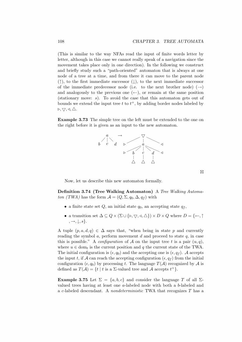
108 CHAPTER 3. TREE AUTOMATA
(This is similar to the way NFAs read the input of finite words letter byletter, although in this case we cannot really speak of a navigation since themovement takes place only in one direction). In the following we constructand briefly study such a “path-oriented” automaton that is always at onenode of a tree at a time, and from there it can move to the parent node(↑), to the first immediate successor (↓), to the next immediate successorof the immediate predecessor node (i.e. to the next brother node) (→)and analogously to the previous one (←), or remain at the same position(stationary move: s). To avoid the case that this automaton gets out ofbounds we extend the input tree t to t+, by adding border nodes labeled by.,5, /,4.
Example 3.73 The simple tree on the left must be extended to the one onthe right before it is given as an input to the new automaton.
a
b c d
→ 5
. a /
. b c d /
4 4 4
£
Now, let us describe this new automaton formally.
Definition 3.74 (Tree Walking Automaton) A Tree Walking Automa-ton (TWA) has the form A = (Q,Σ, q0, ∆, qf ) with
• a finite state set Q, an initial state q0, an accepting state qf ,
• a transition set ∆ ⊆ Q× (Σ∪ {.,5, /,4})×D×Q where D = {←, ↑,→, ↓, s}.
A tuple (p, a, d, q) ∈ ∆ says that, “when being in state p and currentlyreading the symbol a, perform movement d and proceed to state q, in casethis is possible.” A configuration of A on the input tree t is a pair (u, q),where u ∈ domt is the current position and q the current state of the TWA.The initial configuration is (ε, q0) and the accepting one is (ε, qf ). A acceptsthe input t, if A can reach the accepting configuration (ε, qf ) from the initialconfiguration (ε, q0) by processing t. The language T (A) recognized by A isdefined as T (A) = {t | t is a Σ-valued tree and A accepts t+}.
Example 3.75 Let Σ = {a, b, c} and consider the language T of all Σ-valued trees having at least one a-labeled node with both a b-labeled anda c-labeled descendant. A nondeterministic TWA that recognizes T has a

3.5. AUTOMATA OVER TWO-DIMENSIONAL WORDS (PICTURES)109
state set Q = {qa, qb, qc, qr, qf}, where qa, qb, qc mean that the automatonis currently searching for an a, b or c respectively, qr that the pattern wasfound and the automaton is on the way back to the root, and qf is theaccepting state. We choose q0 = qb, i.e. we first navigate down the tree tofind a node with label b, from there a node with label a on the path backto the root, and from there a node with label c somewhere in the subtree.Translated into transitions this procedure is coded as follows:
• search for an appropriate b (i.e. the automaton has to guess that thisb has an a-labeled predecessor) with transitions (qb, σ, ↓ / →, qb)
• on visiting a b switch to state qa and search for an a by using transitions(qb, b, s, qa) and (qa, σ, ↑, qa)
• on visiting an a proceed to qc and search for a c-labeled node in thesubtree with the transitions (qa, a, ↓, qc) and (qc, σ,→ / ↓, qc)
• having visited a c proceed to qr and return to the root by applying thetransitions (qc, c, s, qr) and (qr, σ, ↑, qr)
• accept with the transition (qr,5, s, qf )
£
Regarding the relationship between XML-automata and TWAs and be-tween deterministic and nondeterministic TWAs, the following results havebeen shown up to now.
Theorem 3.76 a) Any TWA can be translated into an equivalent (nonde-terministic) XML-automaton.
b) There exists a language that is recognizable by an XML-automaton butnot by any (nondeterministic) TWA.
c) There exists a language that is recognizable by a nondeterministic TWAbut not by any deterministic TWA.
There are, still, some fundamental questions concerning TWAs that re-main open to computer science; one of those is concerned with complemen-tation: “Is the complement of the tree language recognized by a nondeter-ministic TWA also recognizable by a nondeterministic TWA?” We suspectthat the answer is negative, though.
3.5 Automata over Two-Dimensional Words (Pic-tures)
In this last section of the chapter we are going to take one more furtherstep in generalizing our models by considering two-dimensional words as el-ements of languages and inputs for automata. Strictly speaking, this slightly

110 CHAPTER 3. TREE AUTOMATA
generalized model does not really belong to the area of trees. The essen-tial distinction between them is the fact that trees are the kind of directedgraphs where two pieces of information flow from the root to the leaves ina “spreading” manner, i.e. without being able to converge again into somenode. In other words, in trees a node has always at most one predecessorwhereas in two-dimensional words it has at most two. Still, we are goingto study pictures as a generalized model in this chapter because this verystep of generalization is the one that leads us out of the convenient world ofdecidability and efficient computability as far as it concerns the most funda-mental problems on describing and processing input models. In particular,after introducing automata and MSO-formulas over labeled grids, we aregoing to verify that
a) the class of recognizable picture languages is not closed under comple-ment and
b) the emptiness problem is undecidable.
Definition 3.77 (Picture) A picture over Σ is a pair p = (domp, valp)with
• domp = {1, . . . , m} × {1, . . . , n} for m, n > 1 and
• valp : domp → Σ.
In this case we are speaking of a picture of size (m, n).
Example 3.78 Below we can see a picture of size (2, 3).
a b b
b a b
£
Definition 3.79 (Picture Language) Let Σ++ be the set of all picturesover Σ. Any B ⊆ Σ++ is called a picture language over Σ. If Σ is a singletonset, then we speak of grids [m, n] and grid languages.
Example 3.80 Below we list three basic picture languages that we aregoing to consider in further detail later.
1. for Σ = {a, b}:B1 = {p ∈ Σ++ | p(3, 3) = a, otherwise p(i, j) = b}
2. for Σ = {·}:B2 = {[n, n] | n > 0} (square grids)

3.5. AUTOMATA OVER TWO-DIMENSIONAL WORDS (PICTURES)111
3. for Σ = {a, b}:B3 = {pp | p ∈ Σ++, p is a square}
£
As usual we are going to introduce a model over these pictures thatallows us afterwards to define MSO-formulas, describing languages like theones mentioned above. Models of pictures belonging to a language shouldthen serve as an interpretation for the corresponding MSO-formula.
Definition 3.81 (Pictures as Models) For a picture p of size (m, n) overΣ let
p :=(domp, S
p1 , Sp
2 ,(P p
a
)
a∈Σ
)
with
• Sp1
((i, j), (i + 1, j)
)(lower successor), Sp
2
((i, j), (i, j + 1)
)(right suc-
cessor) for all suitable i, j and
• P pa = {u ∈ domp | valp(u) = a}.
Definition 3.82 (MSO-Logic over Pictures) The MSO-Logic over pic-tures (over Σ) is as previously defined with the atomic formulas:
x = y S1(x, y) S2(x, y) Pa(x) X(y)
The semantics (p, K1, . . . , Kr) |= ϕ(X1, . . . , Xr) where Ki ⊆ domp is definedas usually. For a sentence ϕ we call B(ϕ) = {p ∈ Σ++ | p |= ϕ} the picturelanguage defined by ϕ.
Example 3.83 Consider the language B1 of Example 3.80. First we con-struct an auxiliary formula to specify the symbol at position (0, 0) of thepicture:
topleft(x) = ¬∃yS1(y, x) ∧ ¬∃yS2(y, x)
Now B1 can be defined by the following formula:
∃x1, y1, x2, y2, x3(topleft(x1) ∧ S1(x1, y1) ∧ S2(y1, x2)∧S1(x2, y2) ∧ S2(y2, x3) ∧ Pa(x3) ∧ ∀y(¬y = x3 → Pb(y)))
i.e. by expressing the fact that in the picture there must be a top leftposition from which, after “moving” twice right and twice down, we reachan a-labeled position whereas all other positions are labeled by letter b. £
Example 3.84 Consider the language B2 of Example 3.80. In a squaregrid, departing from the top left position we can reach the bottom rightposition by continuously moving once to the right and once down in an

112 CHAPTER 3. TREE AUTOMATA
alternating fashion. In this sense we can say that a square grid is actuallya picture in which “every set X that contains the top left position and isclosed under diagonal successors also contains the bottom right position”.This is exactly what we express by the following MSO-formula:
∀X[∀x(topleft(x) → X(x))∧∀x∀y∀z(X(x) ∧ S1(x, y) ∧ S2(y, z) → X(z))
→ ∀x(bottomright(x) → X(x))]
where bottomright(x) := ¬∃yS1(x, y) ∧ ¬∃yS2(x, y) £
Now that we have defined a logical formalism to describe picture lan-guages it is time to construct a corresponding automaton-oriented model.To this purpose we first recall the construction we adopted in the case ofconventional trees. The run of a tree automaton is a mapping of states tothe nodes of the input tree. This mapping, along with the labels of thenodes, has to comply with the transitions that the automaton is allowed toperform.
(q2, b) (q1, a) (q0, a)
(q0, a)
(q1, a) (q2, b)
(q0, a)
tree transition
Figure 3.1: Run tree of a tree automaton.
This way, a run is composed by matching the prescribed triangles (al-lowed transitions) to a triangle of nodes (labeled tree node along with bothits immediate successors). Picture acceptors (Tiling-Systems) are nondeter-ministic systems that function in a similar fashion. They guess the assign-ment of states to the input picture and then verify the local correctness ofthe assignment by matching it with the allowed transitions. But this timetransitions are represented by (2 × 2)-squares instead of triangles, as illus-trated by Figure 3.2. Each such possible square of the “filled-out” picturehas to correspond to a transition of Tiling-System. To be able to distinguishthose squares that include some boundary nodes (i.e. belonging to the firstor the last row or column) of the picture, we extend the input by marginalsymbols #, as illustrated by the following example:

3.5. AUTOMATA OVER TWO-DIMENSIONAL WORDS (PICTURES)113
a p
b r
b q
a q
b p
b p
transitions
Figure 3.2: Verification of matching transitions on an assignment of states
# # # # #
# a b b #
# b a b #
# # # # #
Definition 3.85 (Tiling-Systems (T-Systems)) A Tiling-System (T-System) for pictures over Σ has the form A = (Q,Σ, ∆) with a finite set
of states Q and ∆ ⊆[(Σ ∪ {#}) × Q
]4. In other words, a transition is
a tuple of four pairs of the type (input symbol, assigned state). To havea better overview we represent a transition (a1, q1, a2, q2, a3, q3, a4, q4) by a
matrix
(a1q1 a2q2
a3q3 a4q4
)
. A run of A on p =
a1,1 . . . a1,n
.... . .
...am,1 . . . am,n
is a ma-
trix ρ =
q0,0 . . . q0,n+1...
. . ....
qm+1,0 . . . qm+1,n+1
such that, with a0,j = ai,0 = am+1,j =
ai,n+1 := #, the following holds, for all suitable i, j:
(ai,jqi,j ai,j+1qi,j+1
ai+1,jqi+1,j ai+1,j+1qi+1,j+1
)
∈ ∆.
A accepts p if and only if there exists such a run of A on p. As usual wecall the set B(A) := {p ∈ Σ++ | A accepts p} the language recognized bythe t-system A.
Now we are going to consider once again the languages presented inExample 3.80 and this time describe them by t-systems.
Example 3.86 To recognize B1 (the set of all pictures with an a at (3,3)and a b everywhere else) we construct a t-system with states Q = {0, 1, 2}(1 to be assigned to the first and 2 to the second diagonal element) and

114 CHAPTER 3. TREE AUTOMATA
the transitions
(#0 #0#0 b1
)
,
(b1 b0b0 b2
)
,
(b2 b0b0 a0
)
, along with all other
ones that are required to “fill-out” the rest of the picture with state 0.An example run could be (states are denoted as exponents, and state 0 isassumed whenever no state is mentioned):
#0 # # # #
# b1 b b #
# b b2 b #
# b b a0 #
# b b b #
# # # # #
£
Example 3.87 To recognize the square grids required by language B2 ={[m, m] | m > 0} from Example 3.80 we use almost the same trick as whenwe were looking for an appropriate MSO-formula. The idea is to “emit asignal-state” from the top left corner and transmit it through the grid inthe diagonal direction. To this purpose we choose a state set Q = {0, 1}and require the transitions to fit to the picture below (state 0 is assumedwhenever no state is mentioned):
#1 # # # ## ·1 · · ## · ·1 · ## · · ·1 ## # # # #1
The t-system accepts the grid only if it can match its special verification
transition
(·1 #0#0 #1
)
with some part of the input, i.e. if the 1 that was
emitted from the top-left corner is received by the bottom-right corner. £
Remark 3.88 If two languages B1, B2 are both recognizable by t-systems,then the same holds for the languages B1 ∪ B2 and B1 ∩ B2.
The idea for the proof of B1 ∪ B2 is to construct a union of the two t-systems that should have disjoint state sets. For B1 ∩B2 the usual productconstruction has to be applied in order to build a t-system with state setQ1 × Q2.
The last example that we study right away is a more complicated oneand is based on the language B3 of Example 3.80.

3.5. AUTOMATA OVER TWO-DIMENSIONAL WORDS (PICTURES)115
Example 3.89 Let Σ = {a, b} and consider the language B3, namely theset of all pictures over Σ that do not have the form pp for some square p. Apicture p′ belongs to this language if either
1. p′ is not of size (n, 2n), or
2. p′ is indeed of size (n, 2n), but there exist some 1 ≤ i, j ≤ n such thatvalp′(i, j) 6= valp′(i, j + n).
It suffices to construct one t-system for each case because afterwards, byRemark 3.88, we can construct a t-system for the union of these two, whichobviously recognizes B3.
Case 1: Let us first find out how we can accept pictures of size (n, 2n).This can be done by extending the idea of Example 3.87, namely as soon asthe signal state 1 is received by some bottom position it has to be reflectedto the up-right diagonal direction (renamed as signal state 2 to avoid anyconfusion). Now we shall expect to receive the signal state 2 in the top-rightcorner of the grid. Below we can see an accepting run that also shows theother transitions that are required in order to fill out the grid correctly:
#1 #0 #0 #0 #0 #0 #0 #0 #0 #0 #0 #2#0 ·1 ·0 ·0 ·0 ·0 ·0 ·0 ·0 ·0 ·2 #0#0 ·0 ·1 ·0 ·0 ·0 ·0 ·0 ·0 ·2 ·0 #0#0 ·0 ·0 ·1 ·0 ·0 ·0 ·0 ·2 ·0 ·0 #0#0 ·0 ·0 ·0 ·1 ·0 ·0 ·2 ·0 ·0 ·0 #0#0 ·0 ·0 ·0 ·0 ·1 ·2 ·0 ·0 ·0 ·0 #0#0 #0 #0 #0 #0 #0 #0 #0 #0 #0 #0 #0
However, in this example we actually want to accept everything but thiskind of grids. For this purpose, we keep the same t-system and refuse toreceive the signal state 2 at the top-right corner by striking out the transition(
#0 #2·2 #0
)
. Instead, we may receive the signal state 2 everywhere else on
the right or top border by adding the transitions
(#0 #0·2 ·0
)
,
(·0 #0·2 #0
)
(in
case the number of columns is greater or less than 2n, respectively), or wemay receive only the signal state 1 somewhere on the right border by adding
the transitions
(·1 #0·0 #0
)
,
(·1 #0#0 #0
)
,
(·0 #0·1 #0
)
(in case the number of
columns is ≤ n). Of course we expect state 0 in the critical top-right corner
by adding the transition
(#0 #0·0 #0
)
. Finally, some extra consideration has
to be done for the sizes (1, 1) and (1, n), which we skip at this point.

116 CHAPTER 3. TREE AUTOMATA
Case 2: The second t-system has to accept pictures p of size (n, 2n) (wealready know from the previous case how this can be done) that have atleast one pair of positions (i, j), (i, j +n) such that valp(i, j) 6= valp(i, j +n).First of all the t-system has to guess such a position (i, j), which can bedone easily by using nondeterminism. Then, it has to count n positionsto the right to verify that the symbol at (i, j + n) is different. Of coursecounting cannot be done by using n different states because n is not fixed.The idea is depicted below (we assume that (i, j) is a-labeled and (i, j + n)is b-labeled):
a b11
22
2
3a 3a 3a 4a
5 6
7
The position (i, j) is guessed by using the transition
(a1 ∗3a∗1 ∗0
)
. From
there the signal state 1 is emitted vertically towards the bottom borderand the signal state 3a (the a stands for the letter that has been read; itis perfectly in order to do this because the alphabet is finite and given)is emitted horizontally towards position (i, j + n). How do we know thatstate 3a just reached this position to perform the comparison with (i, j)?As soon as state 1 hits the bottom border, it is renamed to 2 and furthertransmitted to the upper right diagonal direction, mainly with the tran-
sitions
(∗1 ∗2#0 #0
)
and
(∗0 ∗2∗2 ∗0
)
. When state 2 crosses the horizontal
transmission of state 3a, they are renamed to 5 and 4a, respectively. The
corresponding transitions are
(∗3a ∗4a∗2 ∗0
)
and
(∗0 ∗5∗4a ∗4a
)
. When state 5
hits the top border, it is renamed to 6 and further transmitted vertically
towards the bottom border, using transitions
(#0 #0∗5 ∗6
)
,
(∗5 ∗6∗0 ∗6
)
and(∗0 ∗6∗0 ∗6
)
. Note that this happens at column j + n because the picture has
n rows and state 2 (later state 5 and 6) took as many steps to the right asto the top. When state 6 crosses the horizontal transmission of state 4a,
the letter comparison is done by transitions
(∗0 ∗6∗4a b7
)
,
(∗4a b7∗0 ∗7
)
. In

3.5. AUTOMATA OVER TWO-DIMENSIONAL WORDS (PICTURES)117
case the letters are different an “OK” signal is transmitted (by using state7) to the bottom and finally to the bottom-right corner with transitions(∗0 ∗7∗0 ∗7
)
,
(∗0 ∗7#0 #7
)
,
(∗7 ∗7#7 #7
)
,
(∗7 #7#7 #7
)
. £
But what about the language B3 of Example 3.80? Is it also recognizableby a t-system as it is the case with its complement? If not, then we wouldhave proven that the closure property under complement does not hold forpicture languages recognizable by t-systems.
Theorem 3.90 The picture language B3 = {pp | p ∈ Σ++, p is a square}is not recognizable by a t-system.
Proof: Towards a contradiction we assume that A = (Q, {a, b}, ∆) recog-nizes B3. Set k := |Q| and consider the runs of A on pictures of size (n, 2n).The number of all possible central stripes (the part of the run consisting ofcolumns n and n+1) in such runs is at most |(Σ∪{#})×Q|2(n+2) = (3k)2n+4.The number of all possible pictures of size (n, n) over Σ is 2n2
. Because thesecond term grows faster than the first one (with respect to n), we can find asuitable n such that 2n2
> (3k)2n+4. For such an n, there exist two picturespp and qq with p 6= q that are both accepted by A with two runs that havethe same central stripes:
%p %′p %q %′q
Combining the left part of the left picture with the right part of the rightone, we can compose a run that accepts pq:
%p %′q
Contradiction. 2
The following theorem summarizes the closure properties that we studiedabove.
Theorem 3.91 The class of picture languages recognizable by t-systems isclosed under union and intersection, but not under complement.
As far as it concerns the relation of t-systems to MSO-logic the followingholds:

118 CHAPTER 3. TREE AUTOMATA
Theorem 3.92 (Giammarresi, Restivo, Seibert, Ths. 1994) A picturelanguage is t-system recognizable if and only if it is EMSO-definable.
Theorem 3.93 (Matz, Schweikardt, Ths. 1997) As the number of al-ternations between second-order quantifiers grows we obtain an infinite hi-erarchy of bigger and bigger classes of picture languages.
Compare the latter result with the case of finite words, where EMSO-logiccan provide the same expressive power as MSO-logic.
We conclude this section (and the whole chapter about trees) by prov-ing that even the most fundamental decision problem on automata is notsolvable within the area of pictures.
Theorem 3.94 The emptiness problem for t-systems is undecidable.
Proof: To prove undecidability, as usual, we consider a reduction of thehalting problem for Turing machines. In other words, we transform a Turingmachine (TM) M to a t-system AM , such that
M halts on the empty tape ⇐⇒ B(AM ) 6= ∅ .
This should suffice to prove that it is not possible to have a method to decidethe emptiness problem for t-systems because, if we had one, then we wouldbe able to decide the halting problem for TMs as well (through the abovementioned transformation), which has been proven to be impossible.
We construct AM in such a way that B(AM ) codes (in its elements)exactly the terminating computations of M when started on the emptytape. Let M = (Q,Σ, q0, ∆, qf ) with à ∈ Σ. ∆ contains transitions ofthe form (q, a, a′, l/r, q′). We suppose that the tape is left bounded. Theconfiguration words are of the form b1 . . . bi−1 (qbi) bi+1 . . . bn (denotingthat M is currently in state q, reading letter b and the rest of the symbols arewritten on the tape to the left and the right of the head). For transitions(q, bi, b
′, l, q′) ∈ ∆ and (q, bi, b′, r, q′) ∈ ∆ the successor configurations are
b1 . . . (q′bi−1) b′ bi+1 . . . bn and b1 . . . bi−1 b′ (q′bi+1) . . . bn, respectively.If we write the sequence of configurations one after the other into the rowsof a table, we obtain a picture of size (m, n), for sufficiently large m, n. Thisway, a terminating computation of M started on the empty tape can berepresented by a picture over Σ ∪ (Q × Σ):
a1,1 . . . a1,n
......
am,1 . . . am,n
with
• a1,1 . . . a1,n = (q0Ã)Ã. . . Ã,

3.5. AUTOMATA OVER TWO-DIMENSIONAL WORDS (PICTURES)119
• ai+1,1 . . . ai+1,n is the word coding a successor configuration of ai,1 . . . ai,n
for 1 ≤ i < m, and
• in am,1 . . . am,n a letter (qfb) occurs.
In the transitions of AM no states are needed because the t-system onlyneeds to verify the correctness of the picture by comparing two consecutiverows and two consecutive positions on the tape (because the Turing machinecan move the head only by one position). For this comparison the 2×2 tilesof the t-system suffice. Hence, the t-system needs the following transitions(we have to assume that the TM is deterministic and complete; otherwise,we have to check that on each row the control state appears only once, whichis possible using 2 states in the system):
For the initial configuration:
(# ## (q0Ã)
)
,
(# #
(q0Ã) Ã
)
,
(# #Ã Ã
)
,
(# #Ã #
)
For the intermediate configurations:
(b (qa)b a′
)
,
(# (qa)# a′
)
,
((qa) ba′ (q′b)
)
, for (q, a, a′, r, q′) ∈ ∆
((qa) ba′ b
)
,
((qa) #a′ #
)
,
(b (qa)
(q′b) a′
)
, for (q, a, a′, l, q′) ∈ ∆
(# a# (qa)
)
,
(a #
(qa) #
)
,
(# a# a
)
,
(a #a #
)
, for a ∈ Σ, q ∈ Q
(a a′
a a′
)
,
(a a′
a (qa′)
)
,
(a a′
(qa) a′
)
, for a, a′ ∈ Σ, q ∈ Q.
For the final configuration:
(# a# #
)
,
(a a′
# #
)
,
(a ## #
)
,
(# (qfa)# #
)
,
((qfa) a′
# #
)
,
(a (qfa′)# #
)
,
((qfa) #
# #
)
for a, a′ ∈ Σ. 2

120 CHAPTER 3. TREE AUTOMATA
3.6 Exercises
Exercise 3.1 Let Σ = Σ0∪Σ2 with Σ0 = Σ2 = {f, g} be a ranked alphabet.Give tree automata for the following languages:
(a) { t ∈ TΣ | on some path in t there are two consecutive occurrences of f }
(b) { t ∈ TΣ | on every path in t there are two consecutive occurrences of f }Remark: a path is always starts at the root and ends at a leaf.
Exercise 3.2 Let the tree languages T1, T2 ⊆ TΣ be recognized by the treeautomata A1,A2, where Ai = (Qi, Σ, δi, Fi) for i = 1, 2. Give tree automatarecognizing the following languages:
(a) TΣ\T1 ,
(b) T1 ∩ T2 .
Exercise 3.3 Let Σ = Σ0 ∪ Σ2 be a ranked alphabet with Σ0 = {c}, Σ2 ={a, b}. Show that
(a) T1 := { t ∈ TΣ | in t there are more a’s than b’s } is not regular,
(b) T2 := { t ∈ TΣ | in t there are more c’s than a’s } is regular.
Exercise 3.4 Let Σ2 = {f}, Σ0 = {a, b}, and
T := { t ∈ TΣ | the frontier word of t is in (ab)+ } .
Give a DTA that recognizes T . Provide also an explanation.Alternatively: Solve the exercise for any regular language L ⊆ {a, b}+ in-stead of (ab)+.
Exercise 3.5 (a) Which language is generated by the following regular ex-pression over Σ0 = Σ2 = {0, 1}?
( 0
c0 c0
)∗c0
·c0[ 1
c1 c1
·c1( 0
c0 c0
)∗c0
·c0 {0}]
(b) Give a regular expression over Σ = Σ0 ∪ Σ2 with Σ0 = {0, 1} andΣ2 = {f} that generates the language
T := { t ∈ TΣ | the frontier word of t contains an infix 01 } .
Exercise 3.6 ∗ Let an almost-deterministic top-down tree automaton be de-fined like a deterministic top-down tree automaton, but with a set Q0 ofinitial states. A run is successful if one of these states is assumed at theroot. Show that there exists a recognizable tree language that cannot berecognized by an almost-deterministic top-down tree automaton.

3.6. EXERCISES 121
Exercise 3.7 Consider the generalized arithmetic expressions with con-stants 0, 1 and the functions + and · with arbitrary arities n ≥ 2. Givean XML-automaton that recognizes the set T0 of all generalized expressionsthat have the value 0 (modulo 3).
Exercise 3.8 (a) Give a deterministic (!) TWA that accepts those inputtrees over Σ = {a, b, c} where an a occurs.Hint: Program a run through the whole input tree.
(b) Give a deterministic TWA for the language T presented in the lecture,namely the set of all Σ-valued trees having at least one a-labeled nodewith both a b-labeled and a c-labeled successor.
Provide an explanation for each part.
Exercise 3.9 Give a t-system that accepts exactly those pictures p overthe singleton alphabet {·} whose domain domp contains an even number ofelements. Provide an explanation.
Exercise 3.10 ∗ Show that the set of square grids [m, m] where m is a primenumber is recognizable by a t-system.

122 CHAPTER 3. TREE AUTOMATA

Chapter 4
Pushdown and CounterSystems
In this chapter we are entering the area of systems whose sets of configu-rations are infinite. This makes it harder to find algorithmic solutions tocertain problems, because we cannot anymore hope to gather all requiredinformation by taking finitely many steps throughout the transition graphof such a system. Nevertheless, we present some methods that successfullysolve the most fundamental problems. We then apply our results to systemsthat are based on recursive structures and gain some significant results.Finally, we identify and prove decidability limits towards more complex sys-tems.
4.1 Pushdown and Counter Automata
It is well known that pushdown automata accept precisely the context-freelanguages. Words are accepted using a finite set of control states and astack as an auxiliary memory. A global state or configuration of such anautomaton is a pair consisting of a control state and a stack content. Hence,different from the finite state systems treated so far, the set of configurationsof a pushdown automaton can be infinite, and therefore new questions arise.
Definition 4.1 A pushdown automaton (PDA) is a tuple A = (Q,Σ, Γ, q0, Z0, ∆)where
• Q is a finite set of control states,
• Σ is a finite input alphabet,
• Γ is a finite stack alphabet,
• q0 ∈ Q is the initial state,
123

124 CHAPTER 4. PUSHDOWN AND COUNTER SYSTEMS
• Z0 ∈ Γ is the initial stack symbol, and
• ∆ ⊆ Q × (Σ ∪ {ε}) × Γ × Γ∗ × Q is the transition relation.
A transition (p, a/ε, Z, β, q) ∈ ∆ is interpreted in the following way: If A isin state p, reading letter a or no input letter respectively, with Z on top ofthe stack, it replaces Z by β and enters control state q.
A configuration is a pair (state q, stack content u) and is often rep-resented by a single word qu, where the first letter of u represents thetop stack symbol. An extended configuration is a triple (state, stack con-tent, remaining input). With a transition (p, a/ε, Z, β, q) ∈ ∆ we reach asuccessor of the current extended configuration (p, Zu, aw) ` (q, βu, w) or(p, Zu, w) ` (q, βu, w) in case the empty word is read. In terms of conven-tional configurations this is written as pZu ` qβu. Hence, we observe thatthe configurations of a PDA induce a prefix rewriting system.
An input word w is accepted by a PDA A if there is a computation ofA on w that starts in q0 with Z0 on the stack, reads all letters of w, andreaches the empty stack at the end of w. In other words, a PDA accepts w iffrom (q0, Z0, w) an extended configuration (q, ε, ε) can be reached in finitelymany steps:
(q0, Z0, w) `∗ (q, ε, ε) for some q ∈ Q .
We call L(A) = {w ∈ Σ∗ | A accepts w} the language recognized by A.
Theorem 4.2 (Main Theorem) A language L is context-free (i. e. can beconstructed by a context-free grammar) iff L is recognizable by a PDA.
We recall three fundamental results from the area of context-free gram-mars. Given a context-free grammar (or two for the third result) G:
1. The word problem “does w belong to L(G)?” is decidable (CYK-algorithm).
2. The emptiness problem “Is L(G) = ∅?” is decidable (marking of thevariables from which a terminal word can be derived).
3. The inclusion and the equivalence problem are both undecidable.
Since PDAs describe the same class of languages as context-free gram-mars, there must be a way to gain analogous results for the former by somereduction to the latter. However, because in computer science PDAs oftenoccur independently (i. e. not related to some grammar), we solve the firsttwo problems directly for PDAs.
Pushdown automata play a central role in various topics in computerscience. In compilers the stack serves as the central data structure. In par-ticular, it is used as an auxiliary memory in the implementation of recursive

4.1. PUSHDOWN AND COUNTER AUTOMATA 125
procedures. In the special case that the stack alphabet consists of a singlesymbol, apart from the initial stack symbol, a stack actually implements acounter. If the stack contains only the initial stack symbol, the number 0 isrepresented. Any other number is represented by the number of occurrencesof the (only) stack symbol on top of the initial one. This again shows thatthe set of all possible stack contents is infinite, as natural numbers are too.
Example 4.3 The depth-first search in a graph G = (V, E), starting froma node v0, can conveniently be implemented by the following recursive pro-cedure DFS(v):
Mark vFor all non-marked successors w of v: DFS(w)
We illustrate this process on the graph below, where v0 = 1, and denotethe nested calls of the algorithm on the left.
DFS(1)DFS(2)
DFS(4)DFS(6)
DFS(5)
1 2 3
6 5 4
To implement this by an iterative program we have to store the procedurecalls in “reverse” direction. This can be done by the following algorithm thatuses a stack as an auxiliary memory:
Initialize stack with v0
Mark v0
As long as the stack is not empty, assume the top symbol is v:if there exists a non-marked neighbor of v:
mark the first non-marked neighbor w of vand push w onto the stack
otherwise, delete v from the stack
If we apply this algorithm to the example graph from above, the stackcontent evolves as follows:
1 → 21 → 421 → 6421 → 421 → 21 → 521 → 21 → 1 → ε .
£
Example 4.4 According to Theorem 4.2, if a language L can be generatedby a context-free grammar, then L is recognizable by a PDA. Suppose L isgenerated by a grammar G. Then w ∈ L iff there exists a derivation tree tfor w in G. While reading w, this can be verified by guessing a left derivationthat corresponds to a depth-first search through the derivation tree. A stackonce again serves as an auxiliary memory for this kind of depth-first search.

126 CHAPTER 4. PUSHDOWN AND COUNTER SYSTEMS
Given the following grammar
S → AA, A → AB | b | c, B → b ,
we suppose that the tree shown below is guessed by a nondeterministicautomaton. On the right we can see how the stack content evolves aftereach step of the depth-first search.
S
A A
A B c
b b
SAA
ABAbBABAbAAc
£
By defining the configurations of a PDA as states of a transition system,we can extend the PDA to an infinite automaton, since there are in generalinfinitely many configurations. This shows again that PDAs can accept awider class of languages than finite automata.
Definition 4.5 [Configuration graph of a PDA] If A is a PDA, then theconfiguration graph of A is defined as GA = (V, (Ea)a∈Σ∪{ε}), where
• V is the set of all configurations reachable from q0Z0, and
• (pZu, qβu) ∈ Ea or (pZu, qβu) ∈ Eε if there is a transition(p, Z, a/ε, β, q) ∈ ∆.
A pushdown graph is the configuration graph of a PDA without ε-transitions.
Example 4.6 We define a PDA A for the language L = {anbn | n > 0}.Let A = ({q0, q1}, {a, b}, {Z0, Z}, q0, Z0, ∆) with
∆ =
(q0, a, Z0, ZZ0, q0), (q0, a, Z, ZZ, q0),(q0, b, Z, ε, q1), (q1, b, Z, ε, q1),(q1, ε, Z0, ε, q1)
.
The configuration graph of A is shown below.
q0Z0a
q0ZZ0a
b
q0ZZZ0a
b
. . .
b
q1 q1Z0ε
q1ZZ0b
q1ZZZ0b . . .b
£

4.1. PUSHDOWN AND COUNTER AUTOMATA 127
The way we defined a PDA at the beginning of the section allows toreplace the top symbol of the stack by several ones (i. e. a word β) in onestep. We say that a PDA is in normal form, if it has only transitions(p, a/ε, Z, β, q) with |β| ≤ 2. That is, in one step the length of the stack canbe increased or reduced by at most 1.
Lemma 4.7 For every PDA there exists an equivalent PDA in normalform.
Proof: For each transition with |β| > 2 add |β|−2 intermediate transitions.2
Every PDA induces a pushdown system, where we suppress the specialroles of q0 and Z0, and ignore the input letters.
Definition 4.8 A pushdown system (PDS) P is a tuple P = (P, Γ, ∆),where P is a finite set of states, Γ is a finite stack alphabet, and ∆ ⊆(P × Γ × P × Γ∗) is a finite set of transition rules, written pa → qv.
A configuration (or global state) of a pushdown system P is a wordpw ∈ P · Γ∗, where the first letter of w represents the top symbol of thestack.
We write
• pw ` p′w′ if w = aw0, w′ = vw0, and pa → p′v ∈ ∆,
• pw `i p′w′ if there exists p0w0, . . . , piwi with pw = p0w0, piwi = p′w′,and pjwj ` pj+1wj+1 for 0 ≤ j < i, and
• pw `∗ p′w′ if pw `i p′w′ for some i ≥ 0.
The configuration graph of a pushdown system P = (P, Γ, ∆) is the graphwith vertex set {c | c ∈ PΓ∗} and an edge between c1 and c2 if c1 ` c2.
Example 4.9 Let P = (P, Γ, ∆) be a PDS, where P = {p0, p1, p2}, Γ ={a, b, c} and ∆ = {(p0a → p1ba), (p1b → p2ca), (p2c → p0b), (p0b → p0ε)}. Asequence of configurations reachable from p2cbba is shown below.
p2cbba ` p0bbba ` p0bba ` p0ba ` p0a ` p1ba ` p2caa ` . . .
£
In the following we consider an extension of pushdown systems to systemsthat have more than one stack.
Definition 4.10 [n-Pushdown System] An n-pushdown system is definedanalogously to a PDS but with n stacks. What needs to be redefined is theway transitions are executed. By [n] we denote the set {1, . . . , n}. Then,

128 CHAPTER 4. PUSHDOWN AND COUNTER SYSTEMS
the transition relation is ∆ ⊆ Q× [n]×Γ×Γ∗×Q. A transition (p, i, a, v, q)means that being in state p with a as the top symbol of stack i, the systemis allowed to replace this a by v and proceed to state q. The configurationsare analogous to the ones of a PDS.
We recall the special case of counter systems and extend them to more thanone counters by giving analogous formal definitions.
Definition 4.11 [Counter System] A counter system is a pushdown systemwhose stack alphabet contains one single symbol Z apart from the initialstack symbol Z0. Hence, the stack content is ZmZ0 and represents thenumber m. A transition (p, Z, v, q) with v ∈ Z∗ means the following:
• for |v| > 1: addition of |v| − 1 and change to state q;
• for |v| = 1: change to state q;
• for |v| = 0: subtraction of 1 and change to state q.
A counter system is deterministic if the corresponding PDS is.
An n-counter system is an n-pushdown system where the stack alphabetfor all stacks contains one single symbol Z apart from the initial stack symbolZ0. A configuration has the form (p, i1, . . . , in), denoting the current stateand the number currently represented by each of the n counters.
Counter systems appear in programming languages, however under a dif-ferent name and format. To study the computation limits on functions overN, register machines were introduced as a model of programming language.
Definition 4.12 [Register Machines (Shepherdson, Sturgis 1963)] An n-register machine is a sequence of instructions 1 I1; 2 I2; . . . ; k Ik (i. e. aprogram) with program variables X1, . . . , Xn. For j < k an instruction Ij
has one of the following forms:
• INC Xi (increase the value of Xi by 1 and proceed to the next instruc-tion);
• DEC Xi (decrease the value of Xi by 1, if possible, and proceed to thenext instruction);
• IF Xi = 0 GOTO m (if the value of Xi = 0, jump to instruction Im,otherwise proceed to Ij+1).
Ik is the instruction STOP. A configuration (j, valueOf(X1), . . . , valueOf(Xn))contains the number j of the instruction that is executed in the next step,and the values currently assigned to each of the n variables.

4.1. PUSHDOWN AND COUNTER AUTOMATA 129
Example 4.13 Consider the register machine R0:
1 IF X2 = 0 GOTO 5;2 INC X1;3 DEC X2;4 IF X3 = 0 GOTO 1;5 STOP
Because (1, x, y, 0) `∗ (5, x+y, 0, 0), R0 can be used to perform the additionof two natural numbers. £
Even if register machines are allowed to perform only the three basicinstructions mentioned above, it can be shown that they possess the sameexpressive power as Turing machines. That is, using only these three in-structions and a finite number of variables one can compute all functionsin number theory. Instead of proving this directly, we conclude this sectionby showing that register machines are indeed only a different formulationof counter systems, and in a later section we reduce Turing machines tocounter systems.
Proposition 4.14 Deterministic counter systems Z in normal form cansimulate register machines R and vice versa.
More specifically, given a counter system Z, there exists a register ma-chine R that comprises the states of Z such that:
Z : (p, i1, . . . , in) `∗ (q, j1, . . . , jn)iff R : (p, i1, . . . , in) `∗ (q, j1, . . . , jn)
The converse direction can be expressed in an analogous way.
Proof (from register machines to counter systems): Given R con-struct Z by using the instruction numbers 1, . . . , k as states and add thefollowing transitions:
• for Ij = INC Xi: (j, i, Z, ZZ, j + 1), (j, i, Z0, ZZ0, j + 1);
• for Ij = DEC Xi: (j, i, Z, ε, j + 1), (j, i, Z0, Z0, j + 1);
• for Ij = IF Xi = 0 GOTO m: (j, i, Z0, Z0, m), (j, i, Z, Z, j + 1).
2
Proof (from counter systems to register machines): For the sake ofsimplicity we exclude complex cases in the transitions of the counter system.We assume that transitions either do not depend on whether the current topstack symbol is Z or Z0, or they leave the stack unchanged (each countersystem can easily be transformed into one satisfying these restrictions).

130 CHAPTER 4. PUSHDOWN AND COUNTER SYSTEMS
Given a deterministic n-counter system Z in normal form, we constructan n + 1-register machine R where we use the last variable as a constantXn+1 = 0 to be able to express static GOTO instructions (i. e. not dependingon the “dynamic” value of a variable). Before proceeding to the constructionwe make the counter system complete by adding transitions such that forevery possible control state and top stack symbol the counter system cantake a step. If Z has the states 1, . . . , k, introduce the instruction numbers1, . . . , 2k + 1 (instruction 2k + 1 is STOP). We denote the static instruction“j IF Xn+1 = 0 GOTO m” by “j GOTO m”. The transition relation is thentransformed to register specific instructions according to the following cases:
• for (j, i, Z/Z0, ZZ/ZZ0, m): 2j − 1 INC Xi; 2j GOTO 2m − 1
• for (j, i, Z, ε, m) and (j, i, Z0, Z0, m): 2j − 1 DEC Xi; 2j GOTO 2m − 1
• for (j, i, Z, Z, m) and (j, i, Z0, Z0, m′):
2j − 1 IF Xi = 0 GOTO 2m′ − 1; 2j GOTO 2m − 1
2
4.2 The Reachability Problem for Pushdown Sys-tems
Configuration graphs of pushdown systems are (in general) infinite. Hencethe question whether one can reach from a configuration c1 a configurationc2 becomes more interesting. We call this the reachability problem. Let Cbe a set of configurations. We define
post∗(C) := {c | c0 `∗ c for some c0 ∈ C}
andpre∗(C) := {c | c `∗ c0 for some c0 ∈ C}.
With this notation the reachability problem for two configurations can berestated in two versions:
• Forward reachability problem: Given c and the definition of C,does c ∈ post∗(C) hold?
• Backwards reachability problem: Given c and the definition of C,does c ∈ pre∗(C) hold?
These formulations can be sharpened to meet a generalized version of thereachability problem. That is, given the definition of some configuration setC, we want to determine the definitions of the configuration sets post∗(C)and pre∗(C). Note that such a result is very helpful for testing certain safetyconditions in system design.

4.2. THE REACHABILITY PROBLEM FOR PUSHDOWN SYSTEMS131
Theorem 4.15 (Buchi 1964) Let P = (P, Γ, ∆) be a PDS and C ⊆ PΓ∗ aregular set of configurations. Then pre∗(C) and post∗(C) are again regular.
Moreover, from an NFA A accepting C we can compute an NFA A ac-cepting pre∗(C) and an NFA A accepting post∗(C).
Before proceeding to the proof, we look at some very significant resultsthat emanate from this theorem.
Corollary 4.16 The stack contents that are reachable from the initial con-figuration q0Z0 of a PDA form a regular set.
Corollary 4.17 The point-to-point reachability problem for pushdown sys-tems is decidable.
Proof: Let c1, c2 be two configurations. Obviously {c2} is a regular set.By using Theorem 4.15 we can determine a DFA that recognizes pre∗({c2}).Then we only need to check whether c1 is accepted by this DFA, in order todecide if c2 is reachable from c1. 2
Since counter systems (and register machines equivalently) are a special-ization of pushdown systems, the same statement as Corollary 4.17 musthold for this case too.
Theorem 4.18 The point-to-point reachability problem for 1-counter sys-tems (equivalently for 1-register machines) is decidable.
Corollary 4.19 The emptiness problem for context-free languages is decid-able.
Proof: We use PDAs (instead of grammars) to prove this corollary. Forthe language recognized by a PDA A the following holds:
L(A) 6= ∅ iff q0Z0 `∗ (q, ε) for some q ∈ Q .
This means that the context-free language is non-empty iff q0Z0 ∈ pre∗(Qε),which can be decided by Theorem 4.15. 2
Proof (of Theorem 4.15): First we have to clarify how we will givedefinitions for sets of configurations. We use special NFAs to represent suchregular sets. Let P = (P, Γ, ∆) be a PDS and C ⊆ PΓ∗ a regular setof configurations. A P -automaton for C is an NFA A = (Q,Γ, P,∆A, F )that accepts from an initial state p ∈ P exactly the words w ∈ Γ∗ such thatpw ∈ C. The control states of P are used as initial states of A. Additionally,it is not allowed in A to have a transition to an initial state.

132 CHAPTER 4. PUSHDOWN AND COUNTER SYSTEMS
Input: A P -automaton A, a PDS P = (P,Γ,∆)
1. A0 := A, i := 0
2. repeat :
3. if pa → p′v ∈ ∆ and Ai : p′v−→ q
4. then add (p, a, q) to Ai to obtain Ai+1
5. i := i + 1
6. until no more transitions can be added.
7. A := Ai
Output: A
Figure 4.1: First Saturation Algorithm
Example 4.20 Consider the pushdown system from Example 4.9 and theconfiguration C = {p0aa}. The P -automaton for C is the following:
A : p2
p0a s1
a s2
p1
£
The idea that we use (proposed by Bouajjani, Esparza, Maler, Hansel,Rossmanith, Schwoon) is a transformation of such an NFA. We consider theregular target set C of configurations of a PDS and suppose that the NFAA(C) accepts qvw with a run q
v−→ rw−→ F . If there exists a rule pa → qv
in the pushdown system, then paw must be accepted by the NFA as well.Therefore we add a transition p
a−→ r to its transition relation.
Let P = (P, Γ, ∆) be a PDS and C ⊆ PΓ∗ a regular set of configura-tions represented by a P -automaton A = (Q,Γ, P,∆A, F ). We present twosaturation algorithms to compute P -automata A and A accepting the setspre∗(C) and post∗(C), respectively.
The first saturation algorithm is shown in Figure 4.1. Example 4.21shows the P -automaton computed by the first saturation algorithm with thepushdown system from Example 4.9 and the P -automaton from Example4.20 as inputs.
Since the number of transitions that can be added to a P -automaton isfinite, the algorithm terminates. For the correctness we have to prove that
pw ∈ pre∗(C) ⇔ A : pw−→ F.

4.2. THE REACHABILITY PROBLEM FOR PUSHDOWN SYSTEMS133
For the direction from left to right we show for n ≥ 0:
pw `n ru ∈ C ⇒ A : pw−→ F.
For n = 0 there is nothing to show. Suppose now that pw `n ru andru ∈ C. We can decompose this sequence into paw′ ` p′vw′ `n−1 ru wherew = aw′ and pa → p′v is a transition of the pushdown system. By the
induction hypothesis we know that A : p′vw′
−−→ F , i. e. there is a state q such
that A : p′v−→ q
w′
−→ F . Hence the saturation rule ensures that there is atransition (p, a, q) ∈ ∆A, and thus pw is accepted by A.
For the converse we have to show a more general claim to make theinduction work. We show that for all pw and all q we have
A : pw−→ q ⇒ ∃p′w′ : A : p′
w′
−→ q and pw `∗ p′w′ (*)
For q ∈ F this yields the original claim because A : p′w′
−→ q then means thatp′w′ ∈ C, and thus pw `∗ p′w′ implies that pw ∈ pre∗(C).
If A : pw−→ q, then there exists i such that Ai : p
w−→ q. We prove (*)by induction on i. For i = 0 the claim obviously holds with p′w′ = pw asA0 = A.
For i > 0 let (p1, a, q1) be the transition that was added by the algorithmto Ai−1 to obtain Ai. This transition is used j times in the run Ai : p
w−→ qfor some j ≥ 0. We prove the induction step for i by another induction, thistime on j. If j = 0, then we get Ai−1 : p
w−→ q and we can directly apply theinduction hypothesis for i.
If j > 0, then we can split the run Ai : pw−→ q at the first position where
the new transition is used as follows (where w = u1au2):
Ai−1 : pu1−→ p1
︸ ︷︷ ︸
(1)
, Ai : p1a−→ q1
︸ ︷︷ ︸
(2)
, Ai : q1u2−→ q
︸ ︷︷ ︸
(3)
.
We can apply the induction hypothesis for i to (1) (i. e. to pu1 and p1). This
means that there is p′1u′1 such that A : p′1
u′1−→ p1 and pu1 `∗ p′1u
′1. As a
P -automaton does not have any transitions leading to an initial state, the
only possibility for A : p′1u′1−→ p1 is u′
1 = ε and p′1 = p1. We get pu1 `∗ p1.Considering (2), the transition (p1, a, q1) was added by the algorithm
because there is a pushdown rule p1a → p2v with Ai−1 : p2v−→ q1. Concate-
nating this run with (3) we obtain the run Ai : p2v−→ q1
u2−→ q in which thetransition (p1, a, q1) is used only j − 1 times. The induction hypothesis on j
yields p′w′ such that A : p′w′
−→ q and p2vu2 `∗ p′w′.Combining this with pu1 `∗ p1 (derived from (1)) and the rule p1a → p2v
we get pw `∗ p1au2 ` p2vu2 `∗ p′w′, proving (*).For the part of Theorem 4.15 concerning post∗(C) we use the same idea.
We suppose we are given a PDS P = (P, Γ, ∆), this time in normal form,

134 CHAPTER 4. PUSHDOWN AND COUNTER SYSTEMS
Input: A P -automaton A and a PDS P = (P,Γ,∆)
1. Set A0 := A and i := 0
2. For each rule r : pa → p′bc add a new state r and a transition (p′, b, r)
3. repeat (Saturation steps):
4. if pa → p′ ∈ ∆ and Ai : pa−→ q then add (p′, ε, q)
5. if pa → p′a′ ∈ ∆ and Ai : pa−→ q then add (p′, a′, q)
6. if r : pa → p′a′a′′ ∈ ∆ and Ai : pa−→ q then add (r, a′′, q)
7. i := i + 1
8. until no more transitions can be added.
9. A := Ai
Output: A
Figure 4.2: Second Saturation Algorithm
i. e. containing only rules pa → q or pa → qb or pa → qbc. We use a P -automaton that recognizes the (regular) configuration set C of P. Supposethat the NFA A(C) accepts paw with a run p
aw−−→ F . If there exists a rulepa → qv in the pushdown system, then we must be able to construct a runq
vw−−→ F in the NFA. If the first transition of the run paw−−→ F is p
a−→ r, thenwe distinguish three cases for a rule pa → qv of the PDS.
1. v = ε: add a transition qε−→ r (now qvw = qw is accepted by the run
qε−→ r
w−→ F );
2. v = b: add a transition qb−→ r (now qvw = qbw is accepted by the run
qb−→ r
w−→ F );
3. v = bc: we have to add some transition “qbc−→ r”. But since the
NFA can process only one letter at a time, we need an intermediatestate rρ for each such rule ρ with |v| = 2. In this case, before startingthe procedure we should first have extended the NFA by a transition
qb−→ rρ. Now we can add the transition rρ
c−→ r, so that the NFA finally
accepts qvw = qbcw by the run qb−→ rρ
c−→ rw−→ F .
The second saturation algorithm is shown in Figure 4.2. Example 4.21shows the P -automaton computed by this algorithm with the same inputsas above.
Since the correctness proof is similar to the one for the first saturationalgorithm, it has been dropped here. 2

4.2. THE REACHABILITY PROBLEM FOR PUSHDOWN SYSTEMS135
Example 4.21 Let P be the pushdown system from Example 4.9. Apply-ing the first saturation algorithm for the P -automaton from 4.20, we obtainthe automaton A accepting pre∗(p0aa).
A : p2
c
p0a
ab
s1a s2
p1
b
b
The automaton A obtained by applying the second saturation algorithmand accepting post∗(p0aa) is shown below.
A : p0a
b,ε
s1a s2
p1b r1
a
a
p2c r2
a
£
Complexity estimation of the first saturation algorithm: For thebackwards reachability problem we are given a PDS P = (P, Γ, ∆) in normalform and a P -automaton A = (Q,Γ, P,∆A, F ). Hence, the length of theinput for the algorithm is |P | + |∆| + |Q| + |∆A|. In the first step of eachloop (see Figure 4.1) we examine the existence of both a rule of the pushdownsystem (there are |∆| many) and a matching run (with some v) in the P -automaton. Because |v| ≤ 2 (normal form), such a run can comprise atmost two transitions. Hence, for each rule in ∆ we have to examine at most|Q|2 runs, which in the worst case sums up to |∆| · |Q|2 checks in each loop.Now because a transition is a combination of a pair of states and a letterof the input alphabet, the loop can be executed at most |P | · |Q| · |Γ| times;more transitions cannot be added to the P -automaton. All in all we get a(polynomial) complexity of |∆| · |P | · |Q|3 · |Γ|.
Complexity estimation of the second saturation algorithm: Theinput is the same as before. In this algorithm we have an additional compu-tational effort that must be carried out before entering the loop (see Figure4.2), in order to extend the P -automaton for each rule that increases the

136 CHAPTER 4. PUSHDOWN AND COUNTER SYSTEMS
stack by one symbol. This can be done as many times as there are rules,namely |∆| times. In each loop and for each rule in ∆ we have to find outin which of the three cases it belongs (at most 3 comparisons) and then finda matching transition (not a run!). In the worst case this can be done in3 · |∆| · |Q| steps. For a similar reason as before the loop can be executed atmost (|P |+ |∆|) · |Q| · |Γ| times. All in all we get a (polynomial) complexityof |∆| + 3 · |∆| · (|P | + |∆|) · |Q|2 · |Γ|.
We conclude this section by recalling what holds about the equivalencetests between two PDAs.
Theorem 4.22 The problem
“Given two PDAs A,B, do A and B recognize the same lan-guage?”
is undecidable. However, it is decidable for deterministic PDAs.
Theorem 4.23 The problem
“Given two PDAs A,B, are A and B bisimilar?”
is decidable.
4.3 Recursive Hierarchical Automata
In the previous section we thoroughly studied the reachability problem forPDSs. In this section we consider a kind of system whose analysis dependson the application of this reachability test. These are the so called “recursivehierarchical systems” which consist of components K0, . . . , Kn that can callone another or even themselves (recursion). The states of such a systemare either “normal” ones or calls of a component Kj . Figure 4.3 shows thesystem K0 that comprises three normal states and two calls, one to itselfand one to a component K1. Calls to components are usually representedas boxes, like in the picture. Unlike the case of Figure 4.3, boxes may have
�
� K0
�
K1
a
K0
Figure 4.3: A recursive hierarchical system.

4.3. RECURSIVE HIERARCHICAL AUTOMATA 137
several inputs and outputs. For the sake of simplicity, we only consider thecase of a single input and output in the following.
The concept which recursive hierarchical systems rely on is of coursewell-known to us from the context-free grammars. The idea of replacing acomponent with several ones (including itself) is represented by the rulesthat imply a substitution of some letter by several ones (including itself).
Example 4.24 Consider the context-free grammar G, defined by the fol-lowing rules:
S → AB | ASB | SS, A → a | cA, B → b | cB .
S generates the bracket words over {A, B}, e. g. AABABBAB. If we imag-ine “A” as “(” and “B” as “)”, then this word corresponds to “(()())()”. Aderivation tree of this word is shown below.
S
S S
A S B A B
S S
A B A B
Finally A is replaced by words in c∗a and B by words in c∗b.The rules of this grammar induce a recursive hierarchical system S (Fig-
ure 4.4) that can sequentially call the components A, B or the componentsA, S, B or the components S, S.
A BS
A B
S S
� �
S
Figure 4.4: A recursive hierarchical system corresponding to the grammarof Example 4.24.
The component A is shown in Figure 4.5, where either a c is selected andA is recursively called, or the call is completed by an a. The component Bis constructed similarly. £

138 CHAPTER 4. PUSHDOWN AND COUNTER SYSTEMS
�
� A
�
c
aA
Figure 4.5: A component of the recursive hierarchical system of Figure 4.4.
Definition 4.25 [Recursive Hierarchical Automaton] A recursive hierarchi-cal automaton over Σ has the form A = (K0, . . . , Kn), where every compo-nent Kj = (Qj , BXj , BIj , ij , ∆j , oj) consists of the following:
• a finite state set Qj ;
• a finite set of boxes BXj ;
• a specification of the box content BIj : BXj → {0, . . . , n}. In partic-ular, BIj(B) = i means that in the component Kj the box B is a callto the component Ki;
• an input state ij and an output state oj ;
• a transition relation ∆j with transitions of the form (p, a, q), (p, ε, B),(B, ε, q), (B, ε, B′) for p, q ∈ Qj , a ∈ Σ, and B, B′ ∈ BXj .
Definition 4.26 [Run of a Recursive Hierarchical Automaton] A run of Ais a sequence p0, b1, p1, b2, p2, . . . , bm, pm of
• states pi from Q =⋃n
j=0 Qj and
• labels bi ∈ Σ ∪ {ε}.
For each segment pi, bi+1, pi+1 of the sequence there is a j ∈ {0, . . . , n} suchthat the following holds:
• (pi, bi+1, pi+1) ∈ ∆j (normal transition), or
• (pi, bi+1, B) ∈ ∆j with B ∈ BXj , BIj(B) = m, and pi+1 = im (a callto component Km), or
• (B, bi+1, pi+1) ∈ ∆j with B ∈ BXj , BIj(B) = m, and pi = om (returnfrom component Km), or
• (B, bi+1, B′) ∈ ∆j with B, B′ ∈ BXj , BIj(B) = m, BIj(B
′) = m′,pi = om, pi+1 = im′ (call to component Km′ , while returning fromcomponent Km).

4.3. RECURSIVE HIERARCHICAL AUTOMATA 139
An accepting run on w is a run from i0 to o0, labeled by the word w. Aaccepts w, if there exists an accepting run of A on w.
Example 4.27 Consider the word ccab and the recursive hierarchical sys-tems of Figures 4.4 and 4.5. By following the upper branch of system S andtwice the lower and then once the upper branch of component A, we getthe following accepting run of ccab (of course we also follow once the upperbranch of component B, which is analogous to A):
iSε−→ iA
c−→ qε−→ iA
c−→ qε−→ iA
a−→ oAε−→ oA
ε−→ oAε−→ iB
b−→ oBε−→ oS .
£
Theorem 4.28 Recursive hierarchical automata recognize exactly the context-free languages.
We skip the proof, since it merely goes by a direct transformation of gram-mars to recursive hierarchical automata and vice versa. The transformationof the first direction was illustrated in Example 4.24.
Naturally, the run of the recursive hierarchical automaton illustratedin the last example motivates the question about the reachability problem;namely, given two states of such an automaton, is there a sequence of tran-sitions to reach one from the other? The following theorem answers thisquestion indirectly by giving an equivalence between recursive hierarchicalautomata and pushdown automata. It is then obvious that we can solve thereachability problem, since we have found an efficient solution for the caseof pushdown automata.
Theorem 4.29 For every recursive hierarchical automaton A an equivalentpushdown automaton can be constructed.
Remark 4.30 1. Theorem 4.29 is a variant of the translation from gram-mars to pushdown automata.
2. With some additional effort we obtain variants of Theorem 4.29 withseveral input and output states.
Proof (of Theorem 4.29): Given a recursive hierarchical automaton A =(K0, . . . , Kn) with Kj = (Qj , BXj , BIj , ij , ∆j , oj), we construct a pushdownautomaton with state set Q =
⋃nj=0 Qj and stack alphabet {Z0}∪
⋃nj=0 BXj .
The main idea of the construction is to store the current Kj-state in thecontrol state of the PDA, and to store on the stack the boxes that are calledin a LIFO fashion. This means that the box that is called is stored on top ofthe stack. This way, the correct information about “where to return” whena call is completed is always available. If only the initial stack symbol Z0
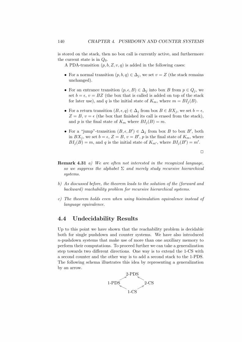
140 CHAPTER 4. PUSHDOWN AND COUNTER SYSTEMS
is stored on the stack, then no box call is currently active, and furthermorethe current state is in Q0.
A PDA-transition (p, b, Z, v, q) is added in the following cases:
• For a normal transition (p, b, q) ∈ ∆j , we set v = Z (the stack remainsunchanged).
• For an entrance transition (p, ε, B) ∈ ∆j into box B from p ∈ Qj , weset b = ε, v = BZ (the box that is called is added on top of the stackfor later use), and q is the initial state of Km, where m = BIj(B).
• For a return transition (B, ε, q) ∈ ∆j from box B ∈ BXj , we set b = ε,Z = B, v = ε (the box that finished its call is erased from the stack),and p is the final state of Km where BIj(B) = m.
• For a “jump”-transition (B, ε, B′) ∈ ∆j from box B to box B′, bothin BXj , we set b = ε, Z = B, v = B′, p is the final state of Km, whereBIj(B) = m, and q is the initial state of Km′ , where BIj(B
′) = m′.
2
Remark 4.31 a) We are often not interested in the recognized language,so we suppress the alphabet Σ and merely study recursive hierarchicalsystems.
b) As discussed before, the theorem leads to the solution of the (forward andbackward) reachability problem for recursive hierarchical systems.
c) The theorem holds even when using bisimulation equivalence instead oflanguage equivalence.
4.4 Undecidability Results
Up to this point we have shown that the reachability problem is decidableboth for single pushdown and counter systems. We have also introducedn-pushdown systems that make use of more than one auxiliary memory toperform their computations. To proceed further we can take a generalizationstep towards two different directions. One way is to extend the 1-CS witha second counter and the other way is to add a second stack to the 1-PDS.The following schema illustrates this idea by representing a generalizationby an arrow.
2-PDS
1-PDS 2-CS
1-CS
4.4. UNDECIDABILITY RESULTS 141
As far as the reachability problem is concerned, the system that is mostlikely to lead us to an undecidability result is the most complex one, namelythe 2-PDS. In the following we first show that this statement indeed holds,and then proceed to proving the same even for a 2-CS, by showing that ithas the same expressive power as a 2-PDS. Hence, we gain the insight thatboth extensions cross the boundaries of decidability and lead us to Turingcomplete systems.
Theorem 4.32 The reachability problem is undecidable for both 2-pushdownsystems and 2-counter systems.
Proof: The proof involves three main steps:
1. From TM to 2-PDS: Given a TM M we construct a 2-PDS PM andconfigurations c0, c1, such that M halts when started on the emptytape iff PM : c0 `∗ c1.
2. From 2-PDS to 4-counter systems: Given a 2-PDS P and configu-rations c0, c1, we construct a 4-counter system Z and configurationsc′0, c
′1 that simulate P, namely: P: c0 `∗ c1 iff Z : c′0 `∗ c′1.
3. From 4-counter systems to 2-counter systems: Given a 4-counter sys-tem Z and configurations c0, c1, we construct a 2-counter system Z ′
and configurations c′0, c′1 that simulate Z, namely: Z : c0 `∗ c1 iff
Z ′ : c′0 `∗ c′1.
1. To simulate a TM we use the two stacks of a 2-PDS to store the tapecontent on the left and on the right of the current working cell. Only theimmediate (left and right) neighbors of the working cell will be directlyaccessible, since they will be the current top symbols of the stacks.
Lemma 4.33 Given a TM M one can construct a 2-PDS PM and config-urations c0, c1, such that M halts when started on the empty tape iff PM :c0 `∗ c1.
Proof: Consider a TM M = (Q,Γ, q0, ∆, qf ) with transitions of the form(p, a, b, R/L/N, q), expressed in colloquial language: “If in state p and read-ing an a on the working tape, print letter b there, move the head to theright / to the left / don’t move, and assume state q”. An M -configurationis of the form [a1 · · · ampb1 · · · bn] with left and right end markers “[” and“]” respectively. The corresponding configuration of the 2-PDS would thenbe (p, b1 · · · bn], am · · · a1[). Hence, we construct a 2-PDS PM = (Q ∪ (Q ×Γ), Γ, ∆′) with “]” and “[” as the initial stack symbol of the first and thesecond stack respectively, and allow the following transitions:

142 CHAPTER 4. PUSHDOWN AND COUNTER SYSTEMS
• for each non-moving transition (p, a, b, N, q) add a PDS transition(p, 1, a, b, q);
• for each right-moving transition (p, a, b, R, q) add the PDS transitions(p, 1, a, ε, (q, b)) and ((q, b), 2, c, bc, q) for all c ∈ Γ;
• for each left-moving transition (p, a, b, L, q) add the PDS transitions(p, 2, c, ε, (p, c)) and ((p, c), 1, a, cb, q) for all c ∈ Γ.
Furthermore we have to ensure that in the end both stacks of the PDS areempty, so that it accepts exactly when the TM reaches a final state. Hence,we have to add transitions that force the PDS to repeatedly erase the topsymbols in both stacks, until it reaches the initial ones (“]” and “[”), namely:
(qf , 1, a, ε, qf ) for a 6= ] and (qf , 2, a, ε, qf ) for a 6= [ .
Now we have ensured that M can reach a certain configuration from anotherone if and only if PM can do the same for the corresponding configurations.Formally:
M : [upv] `∗ [u′qv′] iff PM : (p, v ], uR[) `∗ (q, v′ ], (u′)R[) .
This holds also if one configuration is the initial one (with an empty tape)and the other is a final one:
M : [q0Ã] `∗ [u′qfv′] for some u′, v′ iff PM : (q0, Ã ], [) `∗ (qf , ], [).
In other words, M terminates when started on the empty tape if and onlyif PM can reach the configuration c1 := (qf , ], [) from the configurationc0 := (q0, Ã ], [). 2
2. To simulate a 2-PDS by a 4-counter system, we simulate each push-down stack by a 2-counter system. The following lemma proves that this ispossible.
Lemma 4.34 Given a PDS P and configurations c0, c1, one can constructa 2-counter system ZP and configurations c′0, c
′1, such that P : c0 `∗ c1 iff
ZP : c′0 `∗ c′1.
Proof: To simulate a pushdown stack by two counters we code a stackcontent over a stack alphabet with k elements by a k +1-adic 0-free numbern, carrying the code of the bottom most symbol at the leading position. Weonly illustrate the proof for the case k = 9. Then we can relate each ofthe letters in Γ to a (different) decimal digit (except 0) and map the stackcontent i0 · · · ir to the number with the decimal representation ir · · · i0.

4.4. UNDECIDABILITY RESULTS 143
Example 4.35 Consider an initial stack content 3511. Then
• the stack content 3511 is coded by the number z = 1153;
• the top symbol is the remainder of z after dividing it by 10;
• erasing the top symbol of the stack corresponds to a division by 10without remainder;
• replacing the top symbol of the stack e. g. by 7 corresponds to:division by 10 without remainder, multiplication by 10 and additionof 7;
• replacing the top symbol of the stack e. g. by 27 corresponds to:division by 10 without remainder, multiplication by 10 and additionof 7, multiplication by 10 and addition of 2.
£
These arithmetic operations can easily be carried out by using a secondcounter. We assume that the PDS P = (P, Γ, ∆) is given in normal form.To simplify the construction of the 2-counter system Z, we continue using|Γ| = 9. Every P-transition is carried out by a block of Z-transitions (whichwe will represent by a pseudo program p):
• Erasing the top symbol of the stack (with transition pa → q) is simu-lated by:p: if rem(z1) = a then z1 := z1 div 10, goto q
• Replacing the top symbol of the stack by another symbol (with tran-sition pa → qb) is simulated by:p: if rem(z1) = a then z1 := z1 div 10; z1 := z1 ∗ 10; z1 := z1 + b; gotoq
• Replacing the top symbol of the stack by two symbols (with transitionpa → qbc) is simulated by:p: if rem(z1) = a then z1 := z1 div 10; z1 := z1 ∗ 10; z1 := z1 + c;z1 := z1 ∗ 10; z1 := z1 + b; goto q
We give the counter operations only for the second case. The other twoare analogous. We describe (almost) all of the four operations of this casebelow:
• The computation of rem(z1) can be done with the auxiliary countery1 as follows:
– Subtract 1 from z1 and add 1 to y1, going through the states0, . . . , 9 in a cyclic manner.

144 CHAPTER 4. PUSHDOWN AND COUNTER SYSTEMS
– z1 becomes 0 on reaching state i iff rem(z1) = i. Hence we getthe remainder in the index of the state.
– Now the initial value of z1 is stored in y1, and we can write itback to z1 with the opposite operation, but without changing thestate.
• Multiplication by 10:
– We use 10 auxiliary states and repeat the following until z1 = 0:z1 := z1 − 1 and ten times y1 := y1 + 1. In other words, wedecrease the first counter one by one until it reaches 0, and foreach decrease we perform 10 increases of the second counter.
– Again, we can copy the value of y1 back to z1, simultaneouslyresetting the auxiliary counter to 0.
• Addition of b is easy.
• Division by 10 without remainder is left as an exercise to the reader.
Finally, for the initial configuration c = (p, i0 · · · ir) of the PDS, the cor-responding configuration of the 2-counter system is c′ = (p, (ir · · · i0)10, 9),where 9 is used as the initial stack (counter) symbol. Then, since we havecoded all possible transitions of the PDS by corresponding ones for the 2-counter system, the following holds:
P : c0 `∗ c1 iff ZP : c′0 `∗ c′1 .
2
It follows directly from Lemma 4.34 that any 2-PDS P can be simu-lated by a 4-counter system ZP (actually 3 counters would suffice, sincewe only need one auxiliary counter). For the initial configuration c =(p, i0 · · · ir, j0 · · · js) of P, the corresponding configuration of ZP is thenc′ = (p, (ir · · · i0)10, 9, (js · · · j0)10, 9).
3. The following lemma shows that we can in fact further reduce the num-ber of counters we need.
Lemma 4.36 For every 4-counter system Z and configurations c0, c1, onecan construct a 2-counter system Z ′ and configurations c′0, c
′1, such that
Z : c0 `∗ c1 iff Z ′ : c′0 `∗ c′1.
Proof: To simulate four counters (each with content ki) by two, we code(k1, . . . , k4) by k := 2k1 · 3k2 · 5k3 · 7k4 and store this number in one ofthe counters. Adding, respectively deleting, 1 to k1 then corresponds tomultiplying, respectively dividing, k by 2, and analogously for k2, . . . , k4.

4.5. RETROSPECTION: THE SYMBOLIC METHOD 145
Again these operations can be computed using the second counter as anauxiliary memory. 2
Now that we can simulate a TM by a counter system with two counters,this suffices to show that the reachability problem is undecidable even for2-counter systems. 2
A consequence of Theorem 4.32 is that a programming language withtwo integer variables X1, X2, instructions Xi := Xi +1, Xi := Xi−1, and IFXi = 0 THEN JUMP TO (line) s is already Turing complete, i. e. powerfulenough to simulate every Turing machine.
4.5 Retrospection: The Symbolic Method
In this section we look back at the way we solved the reachability problemfor the different models of automata theory, but this time in a more abstractsense. First of all, it is interesting to note why the reachability problem isso important in system design. The typical problem that we face in suchcases is that we are given a transition system (e. g. a graph) and some set ofstates or configurations (e. g. vertices) in this system. Then, we want to findthe transitive closure under predecessor of this set, i. e. we want to extendthis set in order to additionally include all those states from which, aftera finite number of steps, we can reach the initial designated set. Imaginethat the designated set includes all those states that we want a run to avoid(deadlocks, endless loops, conflicts, etc.). Then of course we also want toavoid the states from which a visit to the “malicious” states can be forced.This is a typical kind of safety constraint that is checked in the frameworkof Model Checking.
Returning once again to the example of a graph, we know that there is avery efficient way to solve this problem, namely by a backwards breadth-firstsearch in time O(|V |+|E|), where V and E are the sets of vertices and edgesof the graph respectively. In fact we cannot hope for a more efficient result.However, if we consider for example a circuit with 100 flip-flops (nothingextraordinary nowadays), the number of different states in this system is2100, which is also the number of steps that our very efficient algorithm hasto take before issuing the result. Hence, even if our method is as good as itgets, it is still not satisfactory enough for large systems.
Since we cannot improve the algorithm itself, our only way out is toimprove the input. Strictly speaking, we have to find a way to improvethe method by which the systems are coded before they are given as aninput to an algorithm. This is exactly the idea of the symbolic method ;instead of enumerating a set of states we can describe it (e. g. by some logicformalism or an automaton) using significantly less space. Then, we canperform a reachability analysis by successively computing the descriptionsof C, pre(C), pre2(C) etc., until no new states can be added anymore. Note

146 CHAPTER 4. PUSHDOWN AND COUNTER SYSTEMS
that this is definitely going to be the case sometime, because the overallnumber of available states in the system is finite anyway.
In the algorithm that is presented below we actually manipulate a for-mula or an automaton until it describes exactly the set that we are lookingfor. We denote
• by β an abstract description (formula or automaton), and
• by [β] the set defined by β.
The symbolic algorithm for backwards reachability takes the following steps:
1. β := description of C;
2. β′ := description of [β] ∪ {q ∈ Q | there is a transition from q to [β]};
3. if [β] = [β′], terminate with output β as a description of pre∗(C);
otherwise β := β′ and back to 2.
We already know that in the case of finite systems on the state space {0, 1}n,it is very convenient to describe sets by boolean formulas β(x1, . . . , xn).
Example 4.37 Consider the state set Q = {0, 1}5 and the designated setof configurations C = {q ∈ Q | 3rd or 5th component = 0}. The set C canbe described by β = ¬x3∨¬x5. In Section 2.2 we studied a way to constructa minimal acyclic automaton for such a boolean formula, namely OBDDs.The OBDD for (the description of) C is shown below.
x3
x5
0 1
£
It is obvious that it is much easier to apply the reachability algorithm onthe level of OBDDs than to apply it on enumerated sets. To achieve this,two steps of the algorithm presented above still remain to be implemented:
1. β′ := description of [β] ∪ {q ∈ Q | there is a transition from q to [β]};
2. the equivalence test (“[β] = [β′]?”).
At this point let us recall that this is exactly what we were striving to-wards when we were trying to solve the reachability problem for pushdownsystems. To describe the given set C we used a P -automaton. To imple-ment the extension to the transitive closure (under predecessor) of C, we

4.6. EXERCISES 147
gradually exhausted the states belonging strictly to pre∗(C) by adding newtransitions to the P -automaton. Furthermore, because we used such a struc-ture, we were not concerned with an equivalence test. The termination ofthe algorithm depended on whether it was possible to add new transitionsto the automaton. What we finally observe is that the reachability analysisof pushdown systems is performed according to the symbolic method, byusing NFAs for the representation of state sets.
We conclude this chapter about pushdown systems by noting that theseare a first essential step in the verification of infinite systems. In such systemswe look at two words u, v, e. g. representing two configurations, and we wantto examine all ways that may lead from the first to the second. To changethe first letter of one word and replace it by another (or two) is only a specialcase.
4.6 Exercises
Exercise 4.1 Show that every PDA A is (language) equivalent to a PDAB that uses only purely expanding and purely reducing transitions.
Exercise 4.2 Let P := (P, Γ, ∆) be a pushdown system with P := {p0, p1},Γ := {a, b, c} and the following set ∆ of transitions:
p0a → p0 p0b → p1c
p0c → p1 p1c → p0bb
Consider the configuration c1 = p0aac. As in the lecture {c1} is accepted byan NFA A with states p0, p1, s1, s2, s3. Apply the saturation procedures tocompute the automata A and A accepting pre∗{c1} and post∗{c1}, respec-tively.
Exercise 4.3 A 1-register machine R decides a set M ⊆ N, if R, initializedwith x ∈ N, always terminates and moreover with value 1 assigned to X1 incase x ∈ M , and with value 0 assigned to X1 in case x 6∈ M .
Show that if M is eventually periodic, then M is decided by a 1-registermachine.
(M is eventually periodic, if for suitable k0, p the following holds:
for all x ≥ k0 : x ∈ M ⇔ x + p ∈ M .)
Exercise 4.4 ∗ Show that the following problem is decidable: Given a push-down automaton A, does there exist a sequence q0Z0 ` q1w1 ` q2w2 ` . . . ofconfigurations such that the length of the configurations is unbounded, i. e.for every n ∈ N there is an i such that |qiwi| > n?
Hint: Consider the repetitions and the following parameters: The num-ber of states n, the number of symbols in the stack alphabet m, and themaximal length of a word v in a transition (p, a/ε, Z, v, q).
148 CHAPTER 4. PUSHDOWN AND COUNTER SYSTEMS
Exercise 4.5 In the lecture we applied the saturation algorithm to com-pute the set pre∗(C) to P -automata whose states from P have no incomingtransitions. Show that this assumption is necessary.
For this purpose, find a pushdown system P := (P, Γ, ∆), a set C ofconfigurations and a P -automaton A that recognizes C and has incomingtransitions into states in P , such that the saturation algorithm computes noautomaton for the set pre∗(C) when applied to A.
Exercise 4.6 Construct a recursive automaton that recognizes the lan-guage generated by the following context-free grammar:
S → aB | bAA → a | aS | bAAB → b | bS | aBB
Give a run of the automaton on the word bbabaa.
Exercise 4.7 ∗ Show that the following problem is undecidable.
Given: A 2-pushdown system P and a configuration c of P.
Question: Does a number n exist, such that |c′| < n holds for all configu-rations c′ ∈ post∗(c)?
The length of the configuration is the sum of the lengths of both stackcontents.
Hint: For a reduction the halting problem for offline Turing machines isrecommended, which can be assumed to be undecidable. (An offline Turingmachine has a read-only input tape and a read-write working tape.)

Chapter 5
Communicating Systems
In this chapter different types of automata are introduced which allow tomodel parallel and distributed computations directly rather than encodingthe behavior of such a system into a single finite state device. We gain asuccinct representation of parallel processes, but also show that one has to becareful not to include too powerful communication possibilities to maintainthe nice properties of finite state machines.
5.1 Synchronized Products
Recall the product construction for NFAs. We generalize this constructionby distinguishing which actions are relevant for which automata.
Definition 5.1 (Synchronized product) Let Ai = (Qi, Σi, q0i, ∆i, Fi)be NFAs for 1 ≤ i ≤ n.. The synchronized product of A1, . . . ,An is theautomaton
A1 ◦ . . . ◦An := (Q1 × . . .×Qn, Σ1 ∪ . . .∪Σn, (q01, . . . , q0n), ∆, F1 × . . .×Fn)
with
((p1, . . . , pn), a, (q1, . . . , qn)
)∈ ∆ :⇔
{
(pi, a, qi) ∈ ∆i for a ∈ Σi and
pi = qi for a 6∈ Σi.
In binary products we usually emphasize the synchronizing alphabet Σ0 :=Σ1 ∩ Σ2 by writing A1 ◦Σ0 A2.
Example 5.2 We model a producer–consumer system by a synchronizedproduct.
1st process: This process models a shipbuilder with two sites for storingships. Possible actions are: produce ship, check the quality, sell a ship,and retake a ship. This process can be implemented by the following
149
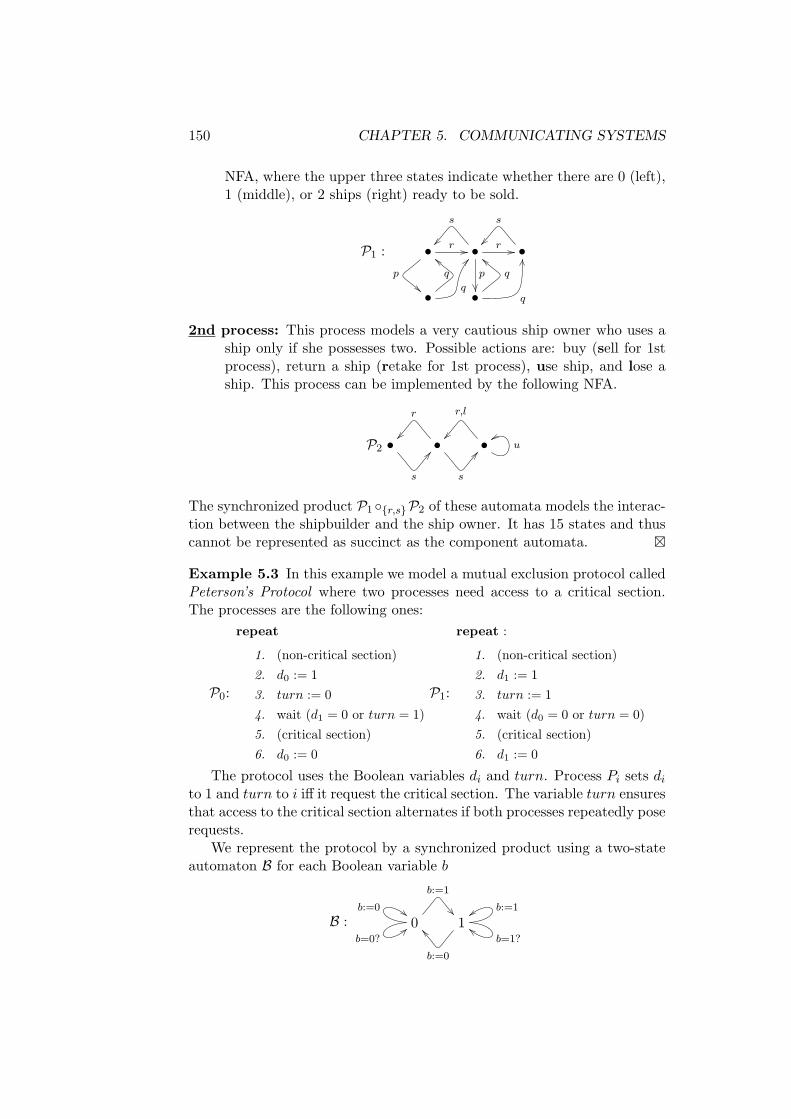
150 CHAPTER 5. COMMUNICATING SYSTEMS
NFA, where the upper three states indicate whether there are 0 (left),1 (middle), or 2 ships (right) ready to be sold.
P1 : • r
p
•
s
r
p
•
s
•q
q •q
q
2nd process: This process models a very cautious ship owner who uses aship only if she possesses two. Possible actions are: buy (sell for 1stprocess), return a ship (retake for 1st process), use ship, and lose aship. This process can be implemented by the following NFA.
P2 •
s
•
s
r
•
r,l
u
The synchronized product P1 ◦{r,s}P2 of these automata models the interac-tion between the shipbuilder and the ship owner. It has 15 states and thuscannot be represented as succinct as the component automata. £
Example 5.3 In this example we model a mutual exclusion protocol calledPeterson’s Protocol where two processes need access to a critical section.The processes are the following ones:
P0:
repeat
1. (non-critical section)
2. d0 := 1
3. turn := 0
4. wait (d1 = 0 or turn = 1)
5. (critical section)
6. d0 := 0
P1:
repeat :
1. (non-critical section)
2. d1 := 1
3. turn := 1
4. wait (d0 = 0 or turn = 0)
5. (critical section)
6. d1 := 0
The protocol uses the Boolean variables di and turn. Process Pi sets di
to 1 and turn to i iff it request the critical section. The variable turn ensuresthat access to the critical section alternates if both processes repeatedly poserequests.
We represent the protocol by a synchronized product using a two-stateautomaton B for each Boolean variable b
B : 0
b:=1
b:=0
b=0?
1
b:=0
b:=1
b=1?

5.1. SYNCHRONIZED PRODUCTS 151
and the following automaton for P0 (P1 is defined analogously):
P0 : 1non-critical section 0
2d0:=1
3
turn:=0
6
d0:=1
5critical section 0
4
turn=1?
d1=0?
Peterson’s Protocol is modeled by the synchronized product P0 ◦ P1 ◦ D0 ◦D1 ◦T . Note that the expanded product automaton has 23 ·62 = 288 states!
£
Example 5.4 We model the famous Dining Philosophers Problem as a syn-chronized product. The problem is the following: 5 philosophers are sittingat a table, and there is a fork in between two of them (as shown below).Each philosopher either thinks or eats, and to eat she needs both of herneighboring forks, i.e. philosopher i needs forks i and i + 1 (mod 5).
F1 P1
P5 F2
F5 P2
P4 F3
F4 P3
A simplified version where we assume that every philosopher picks bothforks simultaneously can be modeled by the synchronized product of
Pi : think
upforks i,i+1
eat
downforks i,i+1
and Fi : down
upforks i,i+1upforks i−1,i
up
downforks i,i+1downforks i−1,i
.
£
The synchronized product of the transition systems presented in theprevious example is only a model for all possible actions (transitions) thatcan occur and for all possible situations (states), in which the group ofphilosophers can find itself at any moment in time. To really describe theproblem of the dining philosophers (there are several versions of it) we haveto construct a protocol that specifies a code of behavior between them byallowing and forbidding certain actions. Such a protocol would for exampleforce the following constraints:

152 CHAPTER 5. COMMUNICATING SYSTEMS
• A deadlock must not occur; that is from every reachable situation, anaction of at least one philosopher is allowed.
• Every philosopher will again and again obtain the forks that are ac-cessible by him (liveliness condition).
• By introducing an intermediate state “hungry” we may require thatwhenever a philosopher gets hungry, he will eventually obtain his forks.
Conditions like the ones above are not modeled in the transition rules of thesystem. They are posed on the behavior of the system, i.e. on the possiblepaths through the graph. A path can be coded by a word, and thus thecondition will specify a subset of all possible words, i.e. a language. Thefirst condition stated above is for example a typical reachability conditionand hence can be expressed by the techniques on finite words that we havelearned so far. For the last condition above one has to examine infiniteexecutions of the system and thus this cannot be expressed by the sametechniques.
In the general case the solution and verification of such problems is re-alized in three different levels. The synchronized product is constructedto describe a language L over the action alphabet representing the possi-ble behavior. The required behavior of the communicating components isdescribed by an automaton for some language K. A solution (protocol)is another automaton recognizing a sub-language L0 ⊆ K. Usually L andK are given, and we have to follow an efficient method to determine L0.Although the synchronized product offers a very compact description of asystem with say k components of n states each, the “state space explo-sion” to the number nk is generally inevitable. Techniques like the symbolicmethod are unfortunately not always helpful, and this is one of the mainproblem of system verification nowadays.
5.2 Communication via FIFO Channels
In this section we introduce finite state machines which communicate witheach other via channels. A channel implements a FIFO queue, i.e messagesare processed in first-in first-out order. We represent the content of a queueby a word a1 . . . an where letters added to the queue are appended to theleft and read from the right.
The basic idea for two automata A1 and A2 and channels c12 andc21 is the following: A1 sends messages to A2 via channel c12 and, viceversa, mathcalA2 sends messages to A1 using channel c12. The contentof a channel cij is a word over a message alphabet Γ. In general au-tomata A1, . . . ,An communicate with each other via a set of channels CN ⊆CNn := ({1, . . . , n}×{1, . . . , n})\{(1, 1), . . . , (n, n)}. For example, if CN =

5.2. COMMUNICATION VIA FIFO CHANNELS 153
{(1, 2), (3, 1), (3, 2)(2, 3)} we obtain the following communication structure:
A1c12 A2
c23A3
c31
c32
Definition 5.5 A communicating finite state machine (CFSM) is a tupleA = (A1, . . . ,An, Γ, CN) where CN ⊆ CNn, Γ is a message alphabet, andfor 1 ≤ i ≤ n Ai = (Qi, Σi, q0i, ∆i, Fi) is a finite automaton with transitionsof the form
• (p, a, q) ∈ Qi × Σi × Qi, (local)
• (p, m!j, q) where p, q ∈ Qi, m ∈ Γ, (i, j) ∈ CN , and (write)
• (p, m?j, q) where p, q ∈ Qi, m ∈ Γ, (j, i) ∈ CN . (read)
A configuration of a CFSM A is a tuple((p1, . . . , pn), (wij)(i,j)∈CN
)where
pi ∈ Qi and wij ∈ Γ∗ is content of channel cij . A configuration of A is alsocalled a global state.
The semantics of the transitions is defined as follows:
(p, (wij)) ` (q, (uij)) :⇔ there exists a k such that
(pk, a, qk) ∈ ∆k andpi = qi for i 6= k,uij = wij for (i, j) ∈ CN
(pk, m!j, qk) ∈ ∆k andpi = qi for i 6= k,ukj = mwkj , uii′ = wii′ for (i, i′) 6= (k, j)
(pk, m?j, qk) ∈ ∆k andpi = qi for i 6= k,ujkm = wjk, uii′ = wii′ for (i, i′) 6= (j, k)
A transition (p, a, q) of an automaton Ai is interpreted as usual, the transi-tions (p, m!j, q) and (p, m?j, q) are used to write, respectively read, a letterfrom the corresponding channel. Note that with this definition of a CFSMonly one component automaton Ai is active at a time. However this can beeasily generalized to real parallel processing.
Remark 5.6 IF a CFSM has bounded channels, i.e. in every execution ofthe system the length of the channel contents is bounded by some l ∈ N, thenthe number of configurations is bounded by |Q1| · . . . · |Qn| · (|Γ| + 1)|CN |·l.Hence such a CFSM is equivalent to an NFA.
A configuration c of a CFSM A is reachable from the initial configuration(q0, ε) (where q0 = (q01, . . . , q0n)) if (q0, ε) ` . . . ` c. Let C be a set ofconfigurations of a CFSM A. If the languages of the channel contents from

154 CHAPTER 5. COMMUNICATING SYSTEMS
C are regular, then C can be finitely represented by tuples consisting of acontrol state and a regular expression rij for the content of channel cij . Wecall such a set a regular set of configurations.
The reachability problem for CFSMs is the following:
Input : A CFSM A, a regular set C of configurations.Problem: Is a configuration c ∈ C reachable from (q0, ε)?
Theorem 5.7 The reachability problem for CFSMs is undecidable.
Proof: We reduce the halting problem for Turing Machines to the reacha-bility problem for CFSMs. Remember that instructions of a Turing machineM are of the form (s, a, a′, ∗, s′) where s, s′ are states of M , a, a′ are symbolsfrom the tape alphabet, and ∗ ∈ {L, R, N} is the direction in which the headof M moves. A configuration of M is a word [usv$ where [ and $ are theleft and right end markers of the tape inscription, u is the word to the left ofthe head of M , v is the word to the right of it (including the symbol beneaththe head), and s is the current state of M . We assume that M only stops ifa special state sfin is reached.
We define an effective transformation of a Turing machine M into aCFSM AM where AM = (AM
1 ,AM2 , {(1, 2), (2, 1)}) such that M stops when
started on the empty tape iff AM reaches a configuration in a set C to bedefined later on.
The idea is that AM1 puts the current configuration of M into channel
c12. AM2 reads this configuration, applying changes to it according to the
instructions of M and sends the new configuration back to AM1 using channel
c21. More precisely:To start the simulation of M , AM
1 puts the initial configuration [s0~$into channel c12, and proceeds to state p0. From thereon AM
1 will writeevery letter read from c21 to channel c12. AM
2 behaves as follows
1. Starting from the initial state read the first three letters a1, a2, a3 fromc12 and store them in a state [a1, a2, a3].
2. If a2 is not a state symbol then
• if a3 = $ write a1, a2, a3 to c21 and enter the initial state again.
• else write a1 to c21, read a letter b from c12 and update the stateto [a2, a3, b].
3. If [a1, a2, a3] = [a, s, b] then 0
• if b = $ write a to c21 and enter state [s, ~, $]
• else if
(i) (s, b, b′, N, s′) ∈ ∆M proceed to state [a, s′, b′]

5.2. COMMUNICATION VIA FIFO CHANNELS 155
(ii) (s, b, b′, R, s′) ∈ ∆M proceed to state [a, b′, s′]
(iii) (s, b, b′, L, s′) ∈ ∆M proceed to state [s′, a, b′] if a 6= [, elsewrite [ to channel c21 and enter state [s′, ~, b′].
Let now C be the set of configurations of the communication state ma-chine AM in which sfin occurs in channel c12. This set is obviously regular.We obtain that the TM M started on the empty tape reaches the stop statesfin iff AM reaches from the initial configuration ((q01, q02), ε, ε) a config-uration in C. Hence the reachability problem for CFSMs is undecidable.
2
This proof can be easily modified such that one single automaton witha channel to itself suffices to simulate Turing machines. We therefore con-clude that the reachability problem is decidable for systems with an un-bounded LIFO memory (stack), but undecidable for systems with an un-bounded FIFO channel.
For the boundedness problem we experience a likewise situation. Inexercise 4.4 we proved that this problem is decidable for pushdown systems.This is unfortunately not the case for a FIFO-communicating automaton.
Theorem 5.8 The problem, whether a FIFO-communicating automaton hasbounded channels starting from a configuration c, is undecidable.
The idea is to consider the decidability of the boundedness problem forthe case of a Turing machine. Since we have already found a way to simulateTMs by CFSMs, the problem is decidable for the former if and only if it isdecidable for the latter.
Lemma 5.9 The boundedness problem for Turing Machines “Given a TMM and a TM-configuration c, is M bounded starting from c?” is undecidable.
Proof: We call a TM M bounded starting from c, in case M reaches onlyfinitely many cells of the working tape, when starting from c. This mayhappen because of two reasons; either M will eventually halt if started fromc, or it will not halt but will move in a bounded area by visiting again andagain the same cells. We know that the first case in undecidable, but weare not sure about the second. For this reason we construct a new TM M ′
that simulates M in such a way that M terminates starting from c iff M ′
is bounded starting from c. This can be done easily by instructing M ′ towork exactly as M and additionally replace the right end marker $ by ~$after each step. Then obviously M halts starting from c iff M ′ is boundedstarting from c. 2
Proof of Theorem 5.8: We use the previous lemma and the constructionfrom the proof of Theorem 5.7. Thus, given M and c we can construct aFIFO-communicating automaton AM such that M is bounded starting from

156 CHAPTER 5. COMMUNICATING SYSTEMS
c iff AM is bounded starting from a configuration where initially c is storedin channel c12. 2
5.3 Message sequence charts
Message sequence charts are a simple formalism for the notation of asyn-chronous communicating processes, their syntax settled in the InternationalStandard Z120.
Definition 5.10 A Message Sequence Chart (MSC) C is given by
• a finite set {P1, . . . , Pn} of processes,
• a finite set M = {m1, . . . , mk} of messages, where each mi involves asend event si and a receive event ri and E = {s1, . . . , sk, r1, . . . , rk} isthe set of all events,
• a label function l : E → {P1, . . . , Pn}, assigning to each event a processsuch that l(si) 6= l(ri), and
• for every 1 ≤ i ≤ n a total order <i defined on the set Ei := {e ∈ E |l(e) = i} of all events belonging to process i (called visual order)
Example 5.11 An MSC is shown in Figure 5.1. In this MSC P = {P1, P2, P3}and e.g. E2 = {r1, s2, s3, r4, s5} with r1 <2 s2 <2 s3 <2 r4 <2 s5.
P1 P2 P3
m1s1 r1m2s2 r2m3s3 r3m4 s4r4
m5 s5r5m6 s6r6
msc C
Figure 5.1: MSC from Example 5.11
£

5.3. MESSAGE SEQUENCE CHARTS 157
Our aim is to assign a semantics to MSCs by defining a partial order onthe send and receive events. To do this we need some facts on partial ordersas a preparation.
Definition 5.12 A partial order over a set A is a relation < ⊆ A×A suchthat
• ¬(a < a) for all a ∈ A (< is irreflexive),
• (a < b) ∧ (b < c) ⇒ a < c for all a, b, c ∈ A (< is transitive), and
• ¬((a < b) ∧ (b < a)
)for all a, b ∈ A (< is acyclic).
Obviously every partial order gives rise to an acyclic graph. Conversely,every acyclic graph (A,→) induces a partial order (A, <) with a < b :⇔there is a non-empty →-path from a to b.
Definition 5.13 Let (A, <) be a partial order. The Hasse diagram (A, <·)of (A, <) is the acyclic graph defined by
a <· b :⇔ a < b and there exists no c ∈ A : a < c < b
A linearization of a partial order (A, <) is a total order (A,≺) such that
a < b ⇒ a ≺ b.
A linearization of a partial order can be obtained algorithmically by a topo-logical sort based on depth-first search.
Example 5.14 Let A := {pants, trousers, socks, shoes, watch, belt, shirt,tie, jacket}. Figure 5.2 shows a Hasse diagram for A such that the associatedpartial order allows to dress correctly. The associated partial order is definedby a < b iff there exists a nonempty path from a to b in the Hasse diagramfor A.
A possible linearization of this partial order is the following:
watch < shirt < tie < pants < trousers < belt < jacket < socks < shoes.
£
Definition 5.15 Let C be an MSC. The semantics of C is the partial orderon the send and receive events of C induced by the acyclic graph (E,→)defined by
e → e′ :⇔ e = sj and e′ = rj , or
e <i e′ and at least one of them is send event, or
e = rj , e′ = rk with l(rj) = l(rk) and sj <i sk.
A race of an MSC C is a pair of receive events r, r′ such that r <i r′ forsome i, but not r < r′ in the partial order induced by (E,→).

158 CHAPTER 5. COMMUNICATING SYSTEMS
pants
socks trousers shirt watch
shoes belt tie
jacket
Figure 5.2: Hasse Diagram for Example 5.14
Example 5.16 Figure 5.3 shows the Hasse diagram of the partial orderdefined by the MSC C from Figure 5.1. Note that r5 and r6 are not orderedin the partial order induced by (E,→), but r5 <1 r6, i.e. r5 and r6 are arace of C. £
An important task when dealing with MSCs is to find all races. Thestandard procedure is to construct the acyclic graph (E,→) from Definition5.15, then compute its transitive closure (E, <), and compare this with thevisual orders <i.
MSCs can be generalized to higher level message sequence charts (HM-SCs), where a HMSC is a directed graph composed of MSCs. A HMSCdefines a family of MSCs, obtained from paths in the HMSC graph by con-catenating the component MSCs.
Example 5.17 Let a HMSC be given by the following graph with compo-nent MSCs as shown in Figure 5.4:
C1
C2 C3
An expansion of this HMSC is shown in Figure 5.5, where the dashed linesindicate that the part between label 1 and 2 can be repeated arbitrarilyoften afterwards. We obtain a family of MSCs with an unbounded set ofraces (for process P3).
£
The previous example leads us to partial orders with a larger and largernumber of nodes. There is a special theory that deals with such partial

5.3. MESSAGE SEQUENCE CHARTS 159
s1
r1
s2
r2
s3
r3
s4
r4
s6
s5
r5
r6
Figure 5.3: Hasse Diagram for the MSC of Figure 5.1
P1 P2 P3
msc C1
P1 P2 P3
msc C2
P1 P2 P3
msc C3
Figure 5.4: Component MSCs for Example 5.17

160 CHAPTER 5. COMMUNICATING SYSTEMS
P1 P2 P3
1
2
Figure 5.5: Expanded HMSC from Example 5.17
orders as trace languages. These represent a generalization of words tolabeled partial orders. They are defined by an independence relation on aconcurrency alphabet. Such an alphabet is of the form (Σ, I) with a set ofletters Σ and an irreflexive relation I ⊆ Σ × Σ. A pair (a, b) ∈ I impliesthat two consecutive occurrences of a and b can be switched. Then, everyword w ∈ Σ∗ defines an equivalence class [w] which is the set of words whichcan be obtained from w by a sequence of switches of neighboring letters a, bwith (a, b) ∈ I. We call [w] a trace (“Mazurkiewicz trace”).
Example 5.18 Let D be the relation (Σ × Σ) \ I. D describes the “de-pendency relation” and contains all pairs (a, b) whose order must not beswitched. (Σ, D) can by given as an undirected graph, e.g. by
a d
b c
In this case, if w = adabcd, then aadbcd ∈ [w] and aabdcd ∈ [w]. £

5.4. EXERCISES 161
5.4 Exercises
Exercise 5.1 Consider the following automata A1 over {a.b} and A2 over{b, c}.
A1 : 1b
2
a
3
b
a
A2 : 4b
5
b
c
6
b
c
(a) Draw the graph of the synchronized product A1 ◦b A2, disregarding thestates that are not reachable from the initial state (1, 4).
(b) Describe (informally or by a regular expression) the language acceptedby A1 ◦b A2.
Exercise 5.2 Consider the synchronized product modeling the five philoso-phers, with automata P1, . . . ,P5 and F1, . . . ,F5 as explained in this chapter.Determine the number of states of this synchronized product. Give an upperbound (as small as you can justify) on the number of reachable states fromthe initial states “think” for the philosophers and “down” for the forks.
Exercise 5.3 (a) Consider the language L defined by the regular expres-sion (b+ac+a)∗. Find an NFA A1 over {a, b} and an NFA A2 over {a, c}such that L is accepted by the synchronized product A1 ◦a A2.
(b) Show that no NFAs A1,A2 as in (a) exist such that the language(b+ac+a)∗ + (c+ab+a)∗ is accepted by their synchronized product A1 ◦a
A2.
Exercise 5.4 Let A1 and A2 be synchronized products of NFAs, each con-sisting of m factor NFAs with n states each. Describe a procedure to testthe equivalence of A1 and A2 and give a bound on the time complexity interms of m and n.
Exercise 5.5 (a) Develop a CFSM A that models the “Five PhilosophersProblem”. A shall consist of component automata P1, . . . ,P5 for thephilosophers and F1, . . . ,F5 for the forks, which are lifted separatelyhere. Pi shall be connected via forward and backward channels to bothFi and Fi+1. In particular your model has to ensure that
(i) no fork can be lifted by two philosophers simultaneously,

162 CHAPTER 5. COMMUNICATING SYSTEMS
(ii) a philosopher can eat iff she possesses both of her forks,
(iii) a philosopher can think iff she possesses no fork, and
(iv) once a fork is requested, a philosopher is not in state “think” any-more.
Explain your construction.
(b) Modify your CFSM such that a philosopher is allowed to drop her re-quest for a fork (because the fork is in use) and go back to state “think”.
Exercise 5.6 In the course it was shown that CFSMs consisting of a sin-gle component automaton A with a channel to itself induces an undecidablereachability problem. (“Given such an A, can it reach from an initial config-uration (q, ε) a configuration (p, w) with control state p and channel contentw?”)
Analyze this problem for the restricted case of a CFSM with an one-lettermessage alphabet Γ = {m}. Justify your answer.
Exercise 5.7 Consider the message sequence chart from Figure 5.6.
P1 P2 P3 P4
Id1
Id2
Req
Check
Ack1
Inf
Interr
Disconn1
Disconn2
msc C
Figure 5.6: MSC for Exercise 5.7
We denote the send events by s(Id1), s(Id2), . . . and the receive eventsby r(Id1), r(Id2), . . ..
(a) Draw the Hasse diagram for the partial order associated with C.

5.4. EXERCISES 163
(b) List the races occurring in C.
(c) Give three linearizations of the events of C.

164 CHAPTER 5. COMMUNICATING SYSTEMS

Chapter 6
Petri Nets
6.1 Basic Definitions
Petri nets are models for concurrent systems and their behavior.
Definition 6.1 A Petri net is a tuple N = (P, T, F ) where P and T arenonempty, finite and disjoint sets of places and transitions, respectively, andF ⊆ P × T ∪ T × P is a flow relation.
A marking of a Petri net N = (P, T, F ) is a function m : P → N thatassigns a number of tokens to a place. If P = {p1, . . . , pn} we also writem = (m1, . . . , mn) for the marking m where mi is the number of tokens onplace pi.
A transition t can be fired (or executed) if there is a token on everyplace with an incoming edge to t. When t is fired, one token is removedfrom every place with an incoming edge to t, and one token is put on everyplace connected to t by an outgoing edge.
In figures we represent places by circles and transitions by bars. Tokens arerepresented by dots inside a place. In the context of concurrent systems theplaces are called resource holders, and tokens are resources.
Example 6.2 The following Petri net models a mutual exclusion protocol
165

166 CHAPTER 6. PETRI NETS
where two processes access a critical section.
•
noncritical section • critical section
•
£
Definition 6.3 Let N = (P, T, F ) be a Petri net. The preset of a transitiont ∈ T is the set •t := {p ∈ P | (p, t) ∈ F}, the postset is the set t• :={p ∈ P | (t, p) ∈ F}. The preset •p and postset p• of a place p ∈ P aredefined analogously. The definitions above generalize to sets of transitionsand sets of places in the usual way, e.g., for a set S ⊆ T of transitions weset S• := {p ∈ P | (t, p) ∈ F for some t ∈ S}.
Let m, m′ be markings of a Petri net N = (P, T, F ). We write
m ≥ m′ :⇔ ∀p ∈ P m(p) ≥ m′(p), and
m > m′ :⇔ ∀p ∈ P m(p) ≥ m′(p) and ∃p : m(p) > m′(p).
Let m be a marking of a Petri net N = (P, T, F ) and t ∈ T . We define
m ¤t m′ :⇔ ∀p ∈ •t : m(p) > 0 and
∀p ∈ P : m′(p) =
m(p) − 1 if p ∈ •t, p /∈ t•
m(p) + 1 if p /∈ •t, p ∈ t•
m(p) otherwise
We write m ¤ m′ if there is a transition t with m ¤t m′. A firing sequencefrom m to m′ is a sequence τ = t1, . . . , tn of transitions such that there aremarkings m0, . . .mn with m0 = m, mn = m′ and mi−1 ¤ti mi for 1 ≤ i ≤ n.We write m¤τ m′ if τ is a firing sequence from m to m′ and m¤
∗ m′ if sucha sequence exists.
We call a marking m a deadlock for N if for all t ∈ T there exists ap ∈ •t with m(p) = 0, i.e., no transition of N can be fired.
A Petri net with initial marking m0 is called unbounded (or unsafe) iffor all K ∈ N there exists a sequence m0 ¤ m1 ¤ m2 ¤ . . . of markings suchthat there is an i with
∑
p∈P mi(p) > K.

6.1. BASIC DEFINITIONS 167
Example 6.4 The following picture illustrates the firing of a transition.
m : • • • •
•
••
m′ : •• ••
•
••
£
Example 6.5 The following Petri net illustrates the modeling power ofPetri nets.
1 • 2 •
a b c
3 4 5
d
Transitions a and b are in conflict, only one of them can be fired at a time.We call such transitions nondeterministic. Transition c can be fired inde-pendently of a and b. We call c concurrent to a and b. If transitions a, cfire, the Petri net ends up in a deadlock. If b, c and d fire repeatedly, moreand more tokens are collected at place 1, i.e., the Petri net is unbounded. £
Example 6.6 The following Petri net models two production lines A andB with two intermediate steps each; the main manufacturing phase and thereset back to the idle state. Production line A requires resources p and q,

168 CHAPTER 6. PETRI NETS
Figure 6.1: A Petri net modeling the problem of five dining philosophers.
whereas production line B needs only q.
p q
A B
£
Example 6.7 Consider the problem of the dining philosophers as it wasdescribed in Example 5.4. The Petri net depicted in Figure 6.1 represents asnapshot of a possible modeling of the system, when only the first philoso-pher holds his forks and eats. £
Example 6.8 Consider a small computer network where three PCs have toshare two printers. These two printers can be represented by an auxiliary

6.2. PETRI NETS AS LANGUAGE ACCEPTORS 169
place that possesses two tokens in the idle case.
• •
If any of the PCs wants to use a printer it must obviously be in an non-printing state and furthermore it has to find at least one of the two tokensin the auxiliary place. After finishing the print job, the token is put back tothe auxiliary place. £
A Petri net with n places p1, . . . , pn and markings in Nn models a vectoraddition system, where a transition t leads from some marking m to a newmarking m′ = m+v, with v ∈ {−1, 0, 1}n. In particular, the i-th componentof v is
• −1, in case pi is in the preset but not in the postset of t,
• 1 in case pi is in the postset but not in the preset of t, and
• 0 otherwise.
In the special case of condition/event nets the markings are also 0-1-vectors.That is, we are only interested whether there is a token at some place ornot, and even if there is more than one token at some place, the number isnormalized to 1, after each update of the marking. The mutual exclusionprotocol in Example 6.2 and the production lines in Example 6.6 are suchspecial cases.
6.2 Petri Nets as Language Acceptors
With a small extension of the original definition Petri nets can be used aslanguage acceptors.

170 CHAPTER 6. PETRI NETS
Definition 6.9 Let N = (P, T, F ) be a Petri net and M−, M+ be finite setsof initial markings and final markings, respectively. Let Σ be an alphabetand l : T → Σ be a labeling function that associates with each transitiona label from Σ. N = (N, M−, M+, l) accepts a word w ∈ Σ∗ if there existsa firing sequence τ = t1, . . . , tn from m− ∈ M− to m+ ∈ M+ such thatl(τ) := l(t1) . . . l(tn) = w. We denote by L(N ) the language recognized bythe Petri net N .
Example 6.10 The following pictures illustrate how to construct from anNFA A a Petri net N with initial marking m− = (1, 0, 0) and final markingfinal marking m+ = (0, 1, 0) accepting the same language.
A : 1
a
a 2
b
3
b
N : a 1•a
2
b
3
b
£
Lemma 6.11 For every regular language L there exists a Petri net N suchthat L = L(N ). 2
The power of Petri nets as language acceptors goes beyond the regular lan-guages.
Example 6.12 Let L = {ancbn | n ≥ 0}. L is a Petri net language acceptedby the following Petri net with initial marking m− = (1, 0, 0) and finalmarking m+ = (0, 0, 1).
1 •a
2 b 3
c

6.2. PETRI NETS AS LANGUAGE ACCEPTORS 171
Reading an yields the marking (1, n, 0), from (1, n, 0) we proceed to (0, n, 1)via c, and via bn from (0, n, 1) to (0, 0, 1). This is the only way to reach(0, 0, 1) from (1, 0, 0). Hence this Petri net accepts L. £
In Figure 6.2 the power of Petri nets as language acceptors is shown. Ex-ample languages are shown that separate the different classes.
CSL
REGPNL CFL
anbncn
ww
wwR
Figure 6.2: On the power of Petri nets as language acceptors
Example 6.13 We know that the language L = {anbncn | n > 0} iscontext-sensitive, but not context-free. To prove its position in the inclusiondiagram of Figure 6.2 we construct the following Petri net:
a b c
a b c
This Petri net accepts L with initial marking m− = (1, 0, 0, 0, 0, 0) and finalmarking m+ = (0, 0, 0, 0, 0, 1). £
The previous examples demonstrate the power of Petri nets in checking thecorrect number of occurrences of a letter. However, Petri nets are weakwhen it comes to checking also the order of occurrences. In the following werealize this situation on the language consisting of the palindromes of evenlength.
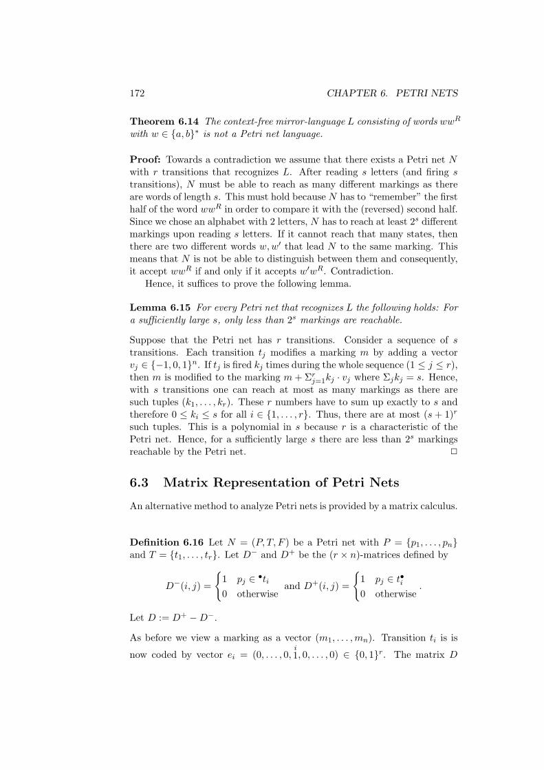
172 CHAPTER 6. PETRI NETS
Theorem 6.14 The context-free mirror-language L consisting of words wwR
with w ∈ {a, b}∗ is not a Petri net language.
Proof: Towards a contradiction we assume that there exists a Petri net Nwith r transitions that recognizes L. After reading s letters (and firing stransitions), N must be able to reach as many different markings as thereare words of length s. This must hold because N has to “remember” the firsthalf of the word wwR in order to compare it with the (reversed) second half.Since we chose an alphabet with 2 letters, N has to reach at least 2s differentmarkings upon reading s letters. If it cannot reach that many states, thenthere are two different words w, w′ that lead N to the same marking. Thismeans that N is not be able to distinguish between them and consequently,it accept wwR if and only if it accepts w′wR. Contradiction.
Hence, it suffices to prove the following lemma.
Lemma 6.15 For every Petri net that recognizes L the following holds: Fora sufficiently large s, only less than 2s markings are reachable.
Suppose that the Petri net has r transitions. Consider a sequence of stransitions. Each transition tj modifies a marking m by adding a vectorvj ∈ {−1, 0, 1}n. If tj is fired kj times during the whole sequence (1 ≤ j ≤ r),then m is modified to the marking m + Σr
j=1kj · vj where Σjkj = s. Hence,with s transitions one can reach at most as many markings as there aresuch tuples (k1, . . . , kr). These r numbers have to sum up exactly to s andtherefore 0 ≤ ki ≤ s for all i ∈ {1, . . . , r}. Thus, there are at most (s + 1)r
such tuples. This is a polynomial in s because r is a characteristic of thePetri net. Hence, for a sufficiently large s there are less than 2s markingsreachable by the Petri net. 2
6.3 Matrix Representation of Petri Nets
An alternative method to analyze Petri nets is provided by a matrix calculus.
Definition 6.16 Let N = (P, T, F ) be a Petri net with P = {p1, . . . , pn}and T = {t1, . . . , tr}. Let D− and D+ be the (r × n)-matrices defined by
D−(i, j) =
{
1 pj ∈ •ti0 otherwise
and D+(i, j) =
{
1 pj ∈ t•i0 otherwise
.
Let D := D+ − D−.
As before we view a marking as a vector (m1, . . . , mn). Transition ti is is
now coded by vector ei = (0, . . . , 0,i1, 0, . . . , 0) ∈ {0, 1}r. The matrix D

6.3. MATRIX REPRESENTATION OF PETRI NETS 173
contains all the information about the “net effect” of transition ti in its i-throw. Suppose ti can be fired from a marking m = (m1, . . . , mn). Then
m ¤ti m′ ⇒ m′ = m + ei · D.
Note that the converse does not hold, i.e.,
m′ = m + ei · D 6⇒ m ¤ti mi′.
Example 6.17 Let N be the following Petri net.
2
t2
4
1
t1
3
t3
Then
D− =
1 1 1 00 0 0 10 0 1 0
and D+ =
1 0 0 00 1 1 00 0 0 1
.
So we obtain
D =
0 −1 −1 00 1 1 −10 0 −1 1
.
Let m = (1, 0, 1, 0) and fire t3. Then we get
(1, 0, 1, 0) + (0, 0, 1) · D = (1, 0, 1, 0) + (0, 0,−1, 1) = (1, 0, 0, 1)
£
Lemma 6.18 If m′ can be reached from m by firing i1 times t1, . . ., ir timestr, then m′ = m + (i1, . . . , ir) · D. 2
As a consequence of the previous lemma we obtain that if m′ is reachablefrom m, then the equation m′ = m + (x1, . . . , xr) · D has a solution in Nr.
As mentioned above, the converse does not hold:

174 CHAPTER 6. PETRI NETS
Example 6.19 Let N be the following Petri net:
1
t1
2
t2
4
3
If m = (1, 0, 0, 0) and m′ = (0, 0, 0, 1), then m′ is not reachable from m, but
(0, 0, 0, 1) = (1, 0, 0, 0) + (x1, x2) ·(−1 1 −1 00 −1 1 1
)
(x1, x2) = (1, 1) is a solution for the equation. £
However, we obtain: If m′ = m + x · D has no solution x, then m′ cannotbe reached from m.
Another application of the matrix representation of Petri nets is moti-vated by applications for balanced distributed systems, where the total ofresources is neither consumed nor expanded.
Definition 6.20 A Petri net N = (P, T, F ) with initial marking m− is saidto be strictly conservative if for all markings m reachable from m− we havem−
1 + . . .+m−n = m1 + . . .+mn. We may write this as m− ·1 = m ·1, where
1 = (1, . . . , 1) ∈ Nn+.
N is called conservative if there is a weight vector w = (w1, . . . , wn) ∈ Nn+
such that m− · w = m · w for every marking m reachable from m−.
Example 6.21 Let N be the following Petri net:
2 • 4
5 •
1 • 3
N is conservative for w = (1, 1, 2, 2, 1) and m− = (1, 1, 0, 0, 1). £
We have the following characterization of conservative Petri nets:

6.4. DECISION PROBLEMS FOR PETRI NETS 175
Lemma 6.22 Let N = (P, T, F ) be a Petri net with initial marking m−
and let P = {p1, . . . , pn} and T = {t1, . . . , tr}. We assume that for everytransition ti there is a marking mi reachable from m− such that ti can be firedfrom mi. Let D be the transition matrix of N and let 0 = (0, . . . , 0) ∈ Nr.Then N is conservative iff the linear equation D · w = 0 has a solutionw ∈ Nn
+.
Proof: Assume that D · w = 0 for some w ∈ Nn+. Let m be some marking
reachable from m−, say, by the firing sequence τ . Let [τ ] be the vector(i1, . . . , ir) where ij is the number of occurrences of tj in τ . By Lemma 6.18,we have m = m− + [τ ] · D. It follows that m · w = (m− + [τ ] · D) · w =m− · w + [τ ] · D · w = m− · w. Hence, N is conservative.
Conversely, assume that N is conservative with weight vector w ∈ Nn+
and let 1 ≤ i ≤ r. By assumption, there are mi, mi with m−¤
∗ mi¤ti mi.
Since both mi, mi are reachable from m−, we obtain m− ·w = mi ·w = mi ·w.By Lemma 6.18, we have mi = mi + ei · D. It follows that mi · w =(mi + ei ·D) ·w = mi ·w + ei ·D ·w and thus, ei ·D ·w = (D ·w)i = 0. Sincei was chosen arbitrarily, we obtain D · w = 0. 2
6.4 Decision Problems for Petri Nets
In this section we investigate important algorithmic issues for Petri nets.
Definition 6.23 The boundedness problem for Petri nets is the following:
Input : A Petri net N , an initial marking m−.Problem: Is there a number K such that for all m reachable from
m− we have∑
p∈P m(p) ≤ K?
The reachability problem for Petri nets is the following:
Input : A Petri net N , an initial marking m− and a final mark-ing m+.
Problem: Is m+ reachable from m− in N?
The covering problem for Petri nets is the following:
Input : A Petri net N , an initial marking m− and a final mark-ing m+.
Problem: Is there a marking m reachable from m− such thatm ≥ m+?
The boundedness of a Petri net N with respect to some initial marking m−
actually guarantees that N can be represented by a finite automaton. Thisholds, because a Petri net with n places that is bounded by some number

176 CHAPTER 6. PETRI NETS
K has only markings (m1, . . . , mn) with Σni=1mi ≤ K. This means that also
mi ≤ K for every i and hence there are less than Kn different markingsreachable in N . These can be represented by the states of a huge, but stillfinite automaton.
In the following we first solve the boundedness problem and then the cov-ering problem. Unfortunately, we have to skip the proof for the decidabilityof the reachability problem because it is far too complex to be presentedhere.
Theorem 6.24 (Karp, Miller 1968) The boundedness problem for Petrinets is decidable.
The proof of this theorem needs some preparation. We first define reacha-bility trees over a Petri net and make some important observations aboutthem.
Definition 6.25 [Reachability Tree of a Petri net] Given a Petri net N andan initial marking m−, the reachability tree t[N, m−] is defined as follows:
• the root of t[N, m−] is m−, and
• the immediate successors of a node m are all markings that are reach-able from m by firing one transition.
Remark 6.26 The reachability tree t[N, m−] contains exactly the markingsthat are reachable from m−.
However, since a place of a Petri net can have arbitrarily many markers,the reachability tree can be infinite. Is there some way to break the (pos-sibly never ending) construction of a reachability tree in order to be ableto perform the boundedness test? The construction of a reachability treefor a Petri net relies on the following monotonicity property. If m is reach-able from m− and there is a nonempty firing sequence τ such that m ¤τ m′
and m ≤ m′, then τ can be fired infinitely often. Two cases have to bedistinguished:
1. If m = m′, then m can be reproduced infinitely often by executing τagain and again.
2. If m < m′, then mi < m′i for some i, and mi can be increased ar-
bitrarily by executing τ again and again. In this case we obtain amonotonically increasing marking sequence m < m′ < m′′ < . . . andconsequently the unboundedness of the Petri net.
Lemma 6.27 (Expansion Lemma) If m−¤
∗m¤∗m′ with m′ > m, then
the following holds: there exist m′′, m′′′ . . . with m−¤
∗ m ¤∗ m′
¤∗ m′′
¤∗
m′′′¤
∗ . . . and m < m′ < m′′ < . . .. Hence, the Petri net is unbounded.

6.4. DECISION PROBLEMS FOR PETRI NETS 177
The algorithm from Figure 6.3 uses the previous observations to compute atruncated reachability tree t(N, m−) for a Petri net N , the Karp-Miller tree.For simplicity we assume that the initial marking m− is not a deadlock. Notethat the marking m′ is possibly changed in line 7 and thus, the conditionsin lines 8 and 9 are checked for this possibly new marking.
Input: A Petri net N = (P, T, F ), an initial marking m−
1. Let m− be an unmarked leaf of t(N,m−)
2. while there are unmarked leafs in t(N,m−) do
3. Choose an unmarked leaf m
4. for m′ such that m ¤ m′ do
5. Add m′ as a new leaf below m
6. if there is a m1 < m′ on the path from m′ to the root
7. do change every m′i> m1
ito ∞ od
8. if m′ already occurs in t(N,m−) do mark it od
9. if m′ is a deadlock do mark it od
10. od
11. od
Output: t(N,m−)
Figure 6.3: Algorithm computing t(N, m−)
As we shall prove in the following the Karp-Miller tree contains all theinformation we need. Note that the structure of the output tree of thealgorithm may depend on the order of chosen leaves in line 3. Further, theremay be m1 < m′ and m2 < m′ with m1 £ m2 and m2 £ m1. The structureof the output tree may also depend on the choice of such a marking in line 6.But nevertheless, the set of all leaf labels for different output trees is alwaysthe same, and this suffices for our purpose.
Example 6.28 The Karp-Miller tree for the Petri net from Example 6.5has the following form:
(1, 1, 0, 0, 0)
ab
c
(0, 1, 1, 0, 0)
c
(1,1,0,61,0)(1,1,0,∞,0)
ab
c
(1, 0, 0, 0, 1)
a
b
(0,0,1,0,1)deadlock
(0,1,1,∞,0)
...
(1,1,0,∞,0)√(1,0,0,∞,1)
...
(0,0,1,0,1)√(1,0,0,61,1)(1,0,0,∞,1)√

178 CHAPTER 6. PETRI NETS
£
Now we have all the knowledge we need to decide whether a Petri net isbounded when started from some given marking. The procedure goes asfollows: Given a Petri net N and an initial marking m− we construct theKarp-Miller tree t(N, m−) by using the algorithm of Figure 6.3. If no ∞ signoccurs in the tree then N is bounded when started from m−. Otherwise, Nis unbounded when started from m−.
To prove the correctness of this method we proceed in two stages. First,we show that the algorithm of Figure 6.3 terminates, i.e., that the Karp-Miller tree is finite, and second that N is unbounded when started from m−
if and only if a ∞ occurs in t(N, m−).
Theorem 6.29 The algorithm from Figure 6.3 computing t(N, m−) termi-nates, i.e., t(N, m−) is finite.
For the proof we need two intermediate results. The first one is the wellknown Konig’s Lemma:
Lemma 6.30 (Konig) Every finitely branching infinite tree has an infinitepath.
Proof: Let t be a finitely branching infinite tree. Starting from the rootr of t we find an infinite path through t by repeatedly picking a son s ofthe current node such that the subtree of t rooted at s is infinite. Since t isassumed to be a finitely branching but infinite, this is always possible. 2
Lemma 6.31 (Dixon) Let V ⊆ Nr be infinite. Then there is an infinitesubset V0 ⊆ V that is totally ordered by ≤.
Proof: We prove this by induction on r. For r = 1 the order ≤ is total,hence there is nothing to show. Assume now that V is an infinite subsetof Nr+1. Let V ′ := {m ∈ Nr | ∃x : (m, x) ∈ V }. Two cases have to bedistinguished:Case 1: V ′ is finite. Then there exists some m0 such that for infinitely manyx we have (m0, x) ∈ V . These vectors form the desired totally ordered set.Case 2: V ′ is infinite. By induction hypothesis there is a totally orderedinfinite subset V ′
0 ⊆ V ′.
a) For some x0 we have x ≤ x0 for all (m, x) ∈ V with m ∈ V ′0 . Then there
exists x1 ≤ x0 such that (m, x1) ∈ V for infinitely many m ∈ V ′0 . These
vectors form the desired infinite totally ordered set.
b) For every (m0, x0) ∈ V with m0 ∈ V ′0 there exists m ∈ V ′
0 and x ∈ N withm > m0 and x > x0 such that (m, x) ∈ V . In this case the existence ofan infinite totally ordered set is trivial.

6.4. DECISION PROBLEMS FOR PETRI NETS 179
2
Proof of Theorem 6.29: Assume that t(N, m−) is infinite. By construc-tion t(N, m−) is finitely branching. Hence, by Konig’s Lemma, t(N, m−)contains an infinite path π. For markings (m1, . . . , mn) appearing on π leti1, . . . , is be those components where eventually ∞ appears. We know that{i1, . . . , is} 6= {1, . . . , n} because otherwise (∞, . . . ,∞) would be reached,then repeated, and therefore π would be finite. So w.l.o.g. assume that af-ter the last ∞ sign has been introduced (this happens after a finite numberof steps!) only markings (m1, . . . , mr,∞, . . . ,∞) (r ≥ 1) appear on π.
By Dixon’s Lemma there exists an infinite totally ordered set V0 of mark-ings of the form (m1, . . . , mr,∞, . . . ,∞) on π. Let m ∈ V0 be the first suchmarking appearing on π. Consider now the markings in V0 appearing afterm on π. Only finitely many of these can be smaller than m. Since V0 isinfinite there must be a m′ appearing after m on π with m′ > m. Henceanother ∞ sign would be introduced by the algorithm, contradicting theassumption above. 2
Now that we proved that the algorithm terminates we have to show thatN is unbounded when started from m− if and only if a ∞ occurs in theKarp-Miller tree t(N, m−).
Direction ⇐: If ∞ occurs in the Karp-Miller tree then m−¤
∗ m ¤∗ m′
with m < m′. According to the expansion lemma we obtain markings m−¤
∗
m′¤
∗ m′′¤
∗ m′′′ . . . with m′ < m′′ < m′′′ . . . Hence, N is unbounded whenstarted from m−.
Direction ⇒: We argue that, if ∞ does not occur in t(N, m−), then Nis bounded when started from m−. According to the construction of thetree, the markings that occur in t(N, m−) are exactly the ones that arereachable from m− (see Remark 6.26), i.e., we have t(N, m−) = t[N, m−].Since the Karp-Miller tree is finite (Theorem 6.29), there are only finitelymany different reachable markings. Hence, N is bounded when started fromm−. 2
The tree t(N, m−) computed by the Algorithm 6.3 can be applied todecide the covering problem mentioned above, the reachability problem ifN is bounded, and other properties like whether there exists a deadlock,or whether N is life (we say that a Petri net is life if for every marking mreachable from m− and for every transition t there is a marking mt that canbe reached from m and where t can be fired).
However, a major drawback of the above mentioned algorithm is that itscomplexity cannot be bounded even by a primitive recursive function.
The result on the reachability problem can be strengthened:
Theorem 6.32 The reachability problem is decidable even for unboundedPetri nets. 2
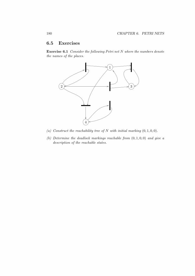
180 CHAPTER 6. PETRI NETS
6.5 Exercises
Exercise 6.1 Consider the following Petri net N where the numbers denotethe names of the places.
1
2 3
4
(a) Construct the reachability tree of N with initial marking (0, 1, 0, 0).
(b) Determine the deadlock markings reachable from (0, 1, 0, 0) and give adescription of the reachable states.

Index
A ◦ B, see synchronized productA/∼, 45A : p
w−→ q, 7AL, 51A, 48AT , 93Aq, 47FOΣ[S, <], 14M(L), 68MSOΣ[S, <], 14Pa(x), 13S(x, y), 13SΣ, 86T (G), 85T (A)
transition monoid, 68tree language, 83
TΣ, 81X(y), 13〈u〉L, 67[m, n], 110[u]L, 51Σ++, 110Σi, 80·c, 94∗c , 95¤t, 166∼L, 51≈L, 67∼T , 92∼A, 50, 93`, 124, 153`∗, 124dom(w), 14domp, 110domt, 82, 103
gsh(L), 38
lc(A), 38
n-counter system, 128
n-pushdown system, 127
n-register machine, 128
p, 111
post∗(C), 130
pre∗(C), 130
pw ` p′w′, 127
rk(a), 80
sh(L), 37
t, 99, 103
t(N, m−), 177•t, 166
t•, 166
t[N, m−], 176
valp, 110
valt, 82, 103
w, 13
wA, 68
algebra, 48
alphabet, 6
ranked, 80
automaton
P -, 131
canonical, 51
complete, 7
deterministic
over trees, 82, 90
over words, 7
XML —, 106
nondeterministic
over trees, 88, 90
over words, 6
XML —, 105
181

182 INDEX
pushdown, 123quotient, 45recursive hierarchical, 138tree walking —, 108
bisimilar, 62bisimulation, 62
equivalence, 62game, 62
winning strategy, 62marking algorithm, 64
boundedness problemfor Petri nets, 175
box, 138
CFSM, 153communicating finite state machine,
153configuration
of a CFSM, 153of a PDA, 124of a PDS, 127
configuration graphof a PDS, 127
congruencefor DFAs, 50Nerode
over trees, 92over words, 51
counter system, 128n-CS, 128
counting language, 35covering problem
for Petri nets, 175
deadlock, 166DFA, 7dining philosophers, 151Dixon’s Lemma, 178DTA, 82↓DTA, 90DTD, document-type definition, 104
emptiness problemfor NTAs, 91
for t-systems, 118error scenario, see model checking
firing sequence, 166
global state, see configurationgrid, 110group-free, 70
Hasse diagram, 157HMSC, 158homomorphism, 44
DFA-, 49NFA-, 45
idempotent, 70
Konig’s Lemma, 178Karp-Miller tree, 177Kripke structure, 30
language, 6counting, 35grid —, 110Kleene closure, 6non-counting, 35Petri net, 170picture —, 110recognizable, 7, 8, 83regular, 83, 97, 105tree —, 81, 97
loop complexity, 38LTL, 32LTS, see transition system
message sequence chart, 156model checking, 28
error scenario, 28monadic second-order, 13monoid
syntactic, 68transition, 68
MSC, 156semantics, 157
MSO0-formulas, 19MSO-Logic, 13
INDEX 183
MSO-logicover pictures, 111over trees, 99, 103
Nerode congruence, see congruenceNFA, 6NTA, 88↓NTA, 90
orderlinearization of, 157partial, 157visual, see MSC
P -automaton, 131PDA, see pushdown automatonPDS, see pushdown system
n-PDS, 127permutation-free, 72Peterson’s protocol, 150Petri net, 165
conservative, 174life, 179marking, 165strictly conservative, 174unbounded, 166unsafe, 166
picture, 110— model, 111
place, see Petri netpostset, 166preset, 166pumping lemma, 87pushdown automaton, 123
configuration, 124configuration graph, 126normal form, 127
pushdown graph, 126pushdown system, 127
race, 157reachability problem
for PDS, 130for CFSM, 154for Petri nets, 175
register machine, 128regular expression, 6
generalized, 26over trees, 95, 97star-free, 31
saturation algorithm, 132first, 132second, 134
star-free, see regular expressionstar-height, 37
generalized, 38symbol, 6
rank of, 80synchronized product, 149syntactic monoid, 68
t-system, tiling system, 113term, see treetoken, see Petri nettransition monoid, 68transition system
labeled, 62pointed, 62
tree, 81Σ-valued, 82, 103— model, 99, 103derivation —, 85Karp-Miller, 177special —, 86
TWA, 108
winning strategy, see bisimulationword model, 13
XML document, 104