Applications of the synchrosqueezing transformin seismic time-frequency analysis

Roberto H. Herrera1, Jiajun Han1, and Mirko van der Baan1

ABSTRACT

Time-frequency representation of seismic signals pro-vides a source of information that is usually hidden in theFourier spectrum. The short-time Fourier transform andthe wavelet transform are the principal approaches to simul-taneously decompose a signal into time and frequency com-ponents. Known limitations, such as trade-offs between timeand frequency resolution, may be overcome by alterna-tive techniques that extract instantaneous modal compo-nents. Empirical mode decomposition aims to decomposea signal into components that are well separated in thetime-frequency plane allowing the reconstruction of thesecomponents. On the other hand, a recently proposed methodcalled the “synchrosqueezing transform” (SST) is an exten-sion of the wavelet transform incorporating elements of em-pirical mode decomposition and frequency reassignmenttechniques. This new tool produces a well-defined time-frequency representation allowing the identification ofinstantaneous frequencies in seismic signals to highlightindividual components. We introduce the SST with applica-tions for seismic signals and produced promising results onsynthetic and field data examples.

INTRODUCTION

This paper is a follow-up study of the empirical mode decompo-sition (EMD) method (Han and Van der Baan, 2013). The EMDmethod is an effective way to decompose a seismic signal into indi-vidual components, called “intrinsic mode functions” (IMFs). EachIMF represents a harmonic signal localized in time, with slowlyvarying amplitudes and frequencies, potentially highlighting differ-ent geologic and stratigraphic information.

EMD methods have evolved from EMD to ensemble EMD (Wuand Huang, 2009) and recently to complete ensemble EMD(CEEMD) (Torres et al., 2011). These extensions aim to solvethe mode mixing problem (Huang et al., 1999, 2003) while keepingthe complete reconstruction capability. Han and Van der Baan(2013) investigate the difference between these EMD methods,and discuss the suitability of EMD for seismic interpretation. Theyconclude that CEEMD not only solves the mode mixing problembut also provides an exact reconstruction of the original signal. Interms of spectral resolution, the EMD-based alternatives outperformthe short-time Fourier transform (STFT) and the wavelet transform(WT) methods. Yet, like other methods, the top-performingCEEMD still has limitations when the components are not well sep-arated in the time-frequency plane.We extend our studies of time-frequency analysis with a recently

proposed transform called the “synchrosqueezing transform” (SST)(Daubechies et al., 2011). SST is a wavelet-based time-frequencyrepresentation that resembles the EMD method. Unlike EMD, ithas a firm theoretical foundation (Wu et al., 2011; Thakur et al.,2013). SST is also an adaptive and invertible transform that im-proves the readability of a wavelet-based time-frequency map usingfrequency reassignment (Auger and Flandrin, 1995), by condensingthe spectrum along the frequency axis (Li and Liang, 2012). Thistransform was originally proposed in the field of audio processing(Daubechies et al., 2011) and has been successfully applied to pa-leoclimate time series (Thakur et al., 2013) and to vibration mon-itoring (Li and Liang, 2012). The SST is still limited by Gabor’suncertainty principle (Hall, 2006), but it approximates the lowerlimit better, thus improving resolution.In this paper, we show the suitability of SST in seismic time-

frequency representation. We contrast and compare SST withCEEMD and the continuous wavelet transform (CWT). Our selec-tion of CEEMD as a reference method for comparison is based onits very low reconstruction errors (Torres et al., 2011) and the factthat it was successfully applied to seismic signal analysis (Han andVan der Baan, 2013), where the instantaneous frequencies are

Manuscript received by the Editor 5 June 2013; revised manuscript received 23 December 2013; published online 12 March 2014.1University of Alberta, Department of Physics, Edmonton, Alberta, Canada. E-mail: rhherrer@ualberta.ca; hjiajun@ualberta.ca; mirko.vanderbaan@

ualberta.ca.© 2014 Society of Exploration Geophysicists. All rights reserved.

V55

GEOPHYSICS, VOL. 79, NO. 3 (MAY-JUNE 2014); P. V55–V64, 11 FIGS.10.1190/GEO2013-0204.1

Dow

nloa

ded

03/1

4/14

to 1

42.2

44.1

91.5

2. R

edis

trib

utio

n su

bjec

t to

SEG

lice

nse

or c

opyr

ight

; see

Ter

ms

of U

se a

t http

://lib

rary

.seg

.org

/

estimated as a posterior step. The CWT is also taken as a referencebecause SST comprises a combination of this method with fre-quency reassignment.In the following section, we describe the theory behind EMD and

the SST. Next, we test the SST on a synthetic example and compareits time-frequency representation and signal reconstruction featureswith the CWT and CEEMD method. Finally, we apply SST on fielddata showing its potential to highlight stratigraphic features withhigh precision.

THEORY

A brief recap of EMD and siblings

EMD is a fully data-driven method to split a signal into compo-nents, called IMFs (Huang et al., 1998). Recursive empirical oper-ations (sifting process; see Huang et al., 1998) separate the signalinto high and low oscillatory components. The sum of all the indi-vidual components reproduces the original signal. However, somemode mixing appears in the classic EMD method, caused by signalintermittency (Huang et al., 1999, 2003), that can produce difficul-ties in interpreting the resulting time-frequency distribution. Thisfact triggered the development of ensemble EMD (Wu and Huang,2009), which is based on a noise-injection technique. Noise isadded prior to decomposition, and ensemble averages are computedfor resulting IMFs. This aids in better separation of independentmodes but does not guarantee perfect reconstruction.Despite the improvement in mode separation using the noise-as-

sisted technique, reconstruction from individual components is im-portant, and Torres et al. (2011) propose an elegant solution. In theCEEMD, an appropriate noise signal is added at each stage of thedecomposition producing a unique signal residual for computingthe next IMF (Torres et al., 2011; Han and Van der Baan, 2013).Computation of the instantaneous frequencies for each IMF thenproduces the desired time-frequency representation (Han andVan der Baan, 2013).

The synchrosqueezing transform

The SSTwas originally introduced in the context of audio signalanalysis and is shown to be an alternative to EMD (Daubechies andMaes, 1996; Daubechies et al., 2011). SST aims to decompose asignal sðtÞ into constituent components with time-varying harmonicbehavior. These signals are assumed to be the addition of individualtime-varying harmonic components yielding

sðtÞ ¼XKk¼1

AkðtÞ cosðθkðtÞÞ þ ηðtÞ; (1)

where AkðtÞ is the instantaneous amplitude, ηðtÞ represents additivenoise, K stands for the maximum number of components in onesignal, and θkðtÞ is the instantaneous phase of the kth component.The instantaneous frequency fkðtÞ of the kth component is esti-mated from the instantaneous phase as

fkðtÞ ¼1

2π

ddt

θkðtÞ: (2)

In seismic signals, the number K of harmonics or components inthe signal is infinite. They can appear at different time slots, with

different amplitudes AkðtÞ, instantaneous frequencies fkðtÞ, andthey may be separated by their spectral bandwidths ΔfkðtÞ.The spectral bandwidth defines the spreading around the central

frequency, which in our case is the instantaneous frequency; seeBarnes (1993) for a completed disentangling of concepts. This mag-nitude is a constraint for traditional time frequency representationmethods. The STFT and the CWT tend to smear the energy of thesuperimposed instantaneous frequencies around their centerfrequencies (Daubechies and Maes, 1996). The smearing equalsthe standard deviation around the central frequency, which is thespectral bandwidth (Barnes, 1993).SST is able to decompose signals into constituent components

with time-varying oscillatory characteristics (Thakur et al., 2013).Thus, by using SST we can recover the amplitude AkðtÞ and theinstantaneous frequency fkðtÞ for each component.

From CWT to SST

The CWT of a signal sðtÞ is (Daubechies, 1992)

Wsða; bÞ ¼1ffiffiffia

pZ

sðtÞψ��t − ba

�dt; (3)

where ψ� is the complex conjugate of the mother wavelet and b isthe time shift applied to the mother wavelet, which is also scaled bya. The CWT is the crosscorrelation of the signal sðtÞ with severalwavelets that are scaled and translated versions of the originalmother wavelet. The symbols Wsða; bÞ are the coefficients repre-senting a concentrated time-frequency picture, which is used to ex-tract the instantaneous frequencies (Daubechies et al., 2011).Daubechies et al. (2011) observe that there is a limit to reduce the

smearing effect in the time-frequency representation using theCWT. Equation 3 can be rewritten using Plancherel’s theorem, en-ergy in the time domain equals energy in the frequency domain, i.e.,Parseval’s theorem in the Fourier domain:

Wsða; bÞ ¼1

2π

Z1ffiffiffia

p sðξÞψ�ðaξÞejbξdξ; (4)

where j ¼ ffiffiffiffiffiffi−1

p, ξ is the angular frequency, and ψðξÞ is the Fourier

transform of ψðtÞ. The scale factor a modifies the frequency of thecomplex wavelet ψ�ðaξÞ, by stretching and squeezing it. Also, thetime shift b is represented by its Fourier pair ejbξ. The convolutionin equation 3 becomes multiplication in the frequency domain inequation 4. Considering the simple case of a single harmonic signalsðtÞ ¼ A cosðωtÞ with Fourier pair sðξÞ ¼ πA½δðξ−ωÞþ δðξþωÞ�,equation 4 can then be transformed into

Wsða; bÞ ¼A2

Z1ffiffiffia

p ½δðξ − ωÞ þ δðξþ ωÞ�ψ�ðaξÞejbξdξ;

¼ A2

ffiffiffia

p ψ�ðaωÞejbω: (5)

In the frequency plane, if the wavelet ψ�ðξÞ is concentratedaround its central frequency ξ ¼ ω0, then Wsða; bÞ will be concen-trated around the scale a ¼ ω0∕ω (the ratio of the central frequencyof the wavelet to the central frequency of the signal). However, whatwe actually get is that Wsða; bÞ often spreads out along the scaleaxis leading to a blurred projection in time-scale representation.

V56 Herrera et al.

Dow

nloa

ded

03/1

4/14

to 1

42.2

44.1

91.5

2. R

edis

trib

utio

n su

bjec

t to

SEG

lice

nse

or c

opyr

ight

; see

Ter

ms

of U

se a

t http

://lib

rary

.seg

.org

/

This smearing mainly occurs in the scale dimension a, for constanttime offset b (Li and Liang, 2012). Daubechies and Maes (1996)show that if smearing along the time axis can be neglected, thenthe instantaneous frequency ωsða; bÞ can be computed as thederivative of the WT at any point ða; bÞ with respect to b, for allWsða; bÞ ≠ 0:

ωsða; bÞ ¼−j

2πWsða; bÞ∂Wsða; bÞ

∂b: (6)

The final step in the new time-frequency representation is to mapthe information from the time-scale plane to the time-frequencyplane. Every point ðb; aÞ is converted to ðb;ωsða; bÞÞ, and this op-eration is called synchrosqueezing (Daubechies et al., 2011). Be-cause a and b are discrete values, we can have a scaling stepΔak ¼ ak−1 − ak for any ak whereWsða; bÞ is computed. Likewise,when mapping from the time-scale plane to the time-frequencyplane ðb; aÞ → ðb; winstða; bÞÞ, the SST Tsðw; bÞ is determined onlyat the centers ωl of the frequency range ½ωl − Δω∕2;ωl þ Δω∕2�,with Δω ¼ ωl − ωl−1:

Tsðωl; bÞ ¼1

Δω

Xak∶jωðak;bÞ−ωlj≤Δω∕2

Wsðak; bÞa−3∕2Δak: (7)

The above equation shows that the new time-frequency represen-tation of the signal Tsðωl; bÞ is synchrosqueezed along the fre-quency (or scale) axis only (Li and Liang, 2012). The SSTreallocates the coefficients of the CWT to get a concentrated imageover the time-frequency plane, from which the instantaneousfrequencies are then extracted (Wu et al., 2011).Following Thakur et al. (2013), the discretized version of

Tsðωl; bÞ in equation 7 is represented by ~T ~sðwl; tmÞ, where tm isthe discrete time tm ¼ t0 þmΔt with Δt the sampling rate andm ¼ 0; : : : ; n − 1; n is total number of samples in the discrete sig-nal ~sm. More special considerations are described in Thakur et al.(2013). The reconstruction of the individual components sk from thediscrete synchrosqueezed transform ~T ~s is then the inverse CWTover a small frequency band lϵLkðtmÞ around the kth component:

skðtmÞ ¼ 2C−1ϕ ℜe

� XlϵLkðtmÞ

~T ~sðwl; tmÞ�; (8)

where Cϕ is a constant dependent on the selected wavelet. As wetake the real partℜe of the discrete SST in that band, we recover thereal component sk. In this paper, we follow Thakur et al. (2013) inwhich the reconstruction is done by a standard least-squares ridgeextraction method; different approaches are explored by Meignenet al. (2012).

Parameter selection

The wavelet choice is a key issue in synchrosqueezing-basedmethods (Meignen et al., 2012). In SST, we first construct thetime-frequency map through a CWT; thus, we need a mother wave-let that satisfies the admissibility condition (i.e., finite energy, zeromean, and bandlimited). At the same time, the wavelet must be agood match for the target signal (Mallat, 2008). By definition, thewavelet coefficients are the correlation coefficients between the tar-get signal and dilated and translated versions of a given basic pattern

(Daubechies, 1992). In our implementation, we use a Morlet wave-let with central frequency and bandwidth estimated from the seismicsignal.The other parameter of interest is the wavelet threshold γ. It ef-

fectively decides the lowest usable magnitude in the CWT (Thakuret al., 2013). It is a noise-based hard thresholding that Thakur et al.(2013) set to 10−8 for the ideal noiseless case in double precisionmachines. In real cases, when the noise level is unknown, it iscommon practice to use the finest scale of the wavelet decomposi-tion (Donoho, 1995) as the noise variance σ2η . This threshold worksin real signals as a noise-level adaptive estimator (Herrera et al.,2006) and is defined as the median absolute deviation (MAD) ofthe first octave (Donoho, 1995; Thakur et al., 2013):

ση ¼ medianðjWsða1∶nv ; bÞ−medianðWsða1∶nv ; bÞÞjÞ∕0.6745; (9)

where Wsða1∶nv ; bÞ are the finest scale wavelet coefficients and0.6745 is a normalizing factor being the MAD of a Gaussian dis-tribution. The threshold is then weighted by the signal length n to beasymptotically optimal with value γ ¼ ffiffiffiffiffiffiffiffiffiffiffiffiffiffiffi

2 log np

· ση.

EXAMPLES

Synthetic data

In this section, we test the SSTwith a challenging synthetic signal(Figure 1). This is the same synthetic example used by Han and Vander Baan (2013). The signal is comprised of an initial 20 Hz cosinewave, with a 100 Hz Morlet atom at 0.3 s, two 30 Hz zero-phaseRicker wavelets at 1.07 and 1.1 s, and three different frequencycomponents between 1.3 and 1.7 s of, respectively, 7, 30, and40 Hz. Note that the 7 Hz frequency component is split into threeparts less than a full period each, appearing at 1.37, 1.51, and 1.65 s.Figure 2a shows the CWT, CEEMD, and SST time-frequency

representations. For comparison purposes, we include the CWT re-sult, because the SST is an extension of the CWT. The STFT isknown to have suboptimal performance, as is shown in Figure 6

0 0.5 1 1.5 2−2

−1.5

−1

−0.5

0

0.5

1

1.5

2

2.5Time series

Time (s)

Am

plitu

de

Figure 1. Synthetic example: background 20 Hz cosine wave,superposed 100 Hz Morlet atom at 0.3 s, two 30 Hz Ricker waveletsat 1.07 and 1.1 s, and there are three different frequency componentsbetween 1.3 and 1.7 s. Same as Figure 1 in Han and Van der Baan(2013).

Seismic time-frequency analysis V57

Dow

nloa

ded

03/1

4/14

to 1

42.2

44.1

91.5

2. R

edis

trib

utio

n su

bjec

t to

SEG

lice

nse

or c

opyr

ight

; see

Ter

ms

of U

se a

t http

://lib

rary

.seg

.org

/

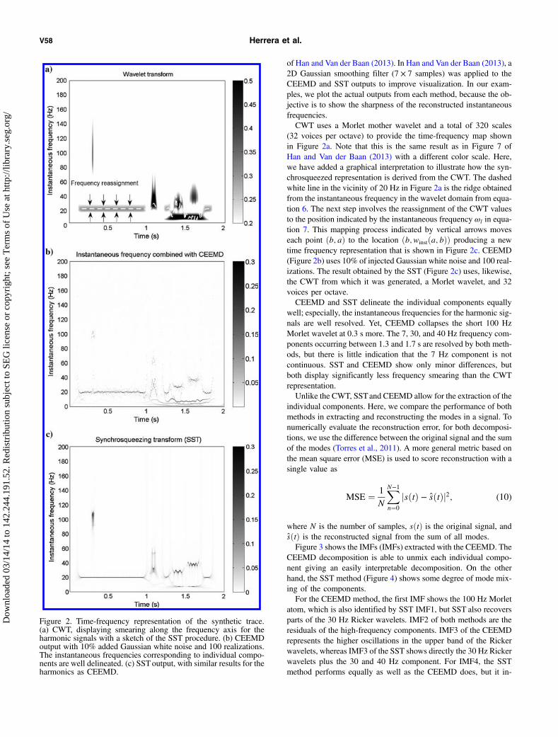
of Han and Van der Baan (2013). In Han and Van der Baan (2013), a2D Gaussian smoothing filter (7 × 7 samples) was applied to theCEEMD and SST outputs to improve visualization. In our exam-ples, we plot the actual outputs from each method, because the ob-jective is to show the sharpness of the reconstructed instantaneousfrequencies.CWT uses a Morlet mother wavelet and a total of 320 scales

(32 voices per octave) to provide the time-frequency map shownin Figure 2a. Note that this is the same result as in Figure 7 ofHan and Van der Baan (2013) with a different color scale. Here,we have added a graphical interpretation to illustrate how the syn-chrosqueezed representation is derived from the CWT. The dashedwhite line in the vicinity of 20 Hz in Figure 2a is the ridge obtainedfrom the instantaneous frequency in the wavelet domain from equa-tion 6. The next step involves the reassignment of the CWT valuesto the position indicated by the instantaneous frequency ωl in equa-tion 7. This mapping process indicated by vertical arrows moveseach point ðb; aÞ to the location ðb; winstða; bÞÞ producing a newtime frequency representation that is shown in Figure 2c. CEEMD(Figure 2b) uses 10% of injected Gaussian white noise and 100 real-izations. The result obtained by the SST (Figure 2c) uses, likewise,the CWT from which it was generated, a Morlet wavelet, and 32voices per octave.CEEMD and SST delineate the individual components equally

well; especially, the instantaneous frequencies for the harmonic sig-nals are well resolved. Yet, CEEMD collapses the short 100 HzMorlet wavelet at 0.3 s more. The 7, 30, and 40 Hz frequency com-ponents occurring between 1.3 and 1.7 s are resolved by both meth-ods, but there is little indication that the 7 Hz component is notcontinuous. SST and CEEMD show only minor differences, butboth display significantly less frequency smearing than the CWTrepresentation.Unlike the CWT, SSTand CEEMD allow for the extraction of the

individual components. Here, we compare the performance of bothmethods in extracting and reconstructing the modes in a signal. Tonumerically evaluate the reconstruction error, for both decomposi-tions, we use the difference between the original signal and the sumof the modes (Torres et al., 2011). A more general metric based onthe mean square error (MSE) is used to score reconstruction with asingle value as

MSE ¼ 1

N

XN−1

n¼0

jsðtÞ − sðtÞj2; (10)

where N is the number of samples, sðtÞ is the original signal, andsðtÞ is the reconstructed signal from the sum of all modes.Figure 3 shows the IMFs (IMFs) extracted with the CEEMD. The

CEEMD decomposition is able to unmix each individual compo-nent giving an easily interpretable decomposition. On the otherhand, the SST method (Figure 4) shows some degree of mode mix-ing of the components.For the CEEMD method, the first IMF shows the 100 Hz Morlet

atom, which is also identified by SST IMF1, but SST also recoversparts of the 30 Hz Ricker wavelets. IMF2 of both methods are theresiduals of the high-frequency components. IMF3 of the CEEMDrepresents the higher oscillations in the upper band of the Rickerwavelets, whereas IMF3 of the SST shows directly the 30 Hz Rickerwavelets plus the 30 and 40 Hz component. For IMF4, the SSTmethod performs equally as well as the CEEMD does, but it in-

Figure 2. Time-frequency representation of the synthetic trace.(a) CWT, displaying smearing along the frequency axis for theharmonic signals with a sketch of the SST procedure. (b) CEEMDoutput with 10% added Gaussian white noise and 100 realizations.The instantaneous frequencies corresponding to individual compo-nents are well delineated. (c) SSToutput, with similar results for theharmonics as CEEMD.

V58 Herrera et al.

Dow

nloa

ded

03/1

4/14

to 1

42.2

44.1

91.5

2. R

edis

trib

utio

n su

bjec

t to

SEG

lice

nse

or c

opyr

ight

; see

Ter

ms

of U

se a

t http

://lib

rary

.seg

.org

/

cludes the 20 Hz component between the two 30 Hz. IMF5 of theCEEMD shows the 20 Hz component with some mixtures of the30 Hz Ricker wavelets, whereas the SST shows a better represen-tation of the 20 Hz with the 7 Hz mode. IMF6 is only informativefor CEEMD with an isolated 7 Hz mode. The remainder are small-valued elements. These low-amplitude components in the CEEMDmethod are low-amplitude frequency bands, derived during the sift-ing process. IMFs are derived from the highest oscillating compo-nents to the lower frequency ones. Like the Fourier transform, someIMFs will have higher amplitudes than other components depend-ing on the signal characteristics. This is visible in Figure 3, wherethe second IMF has not only a different frequency content from IMF1 and 3, but also a different maximum amplitude.The reconstructed signals by both methods are shown in Figure 5.

CEEMD (top dotted gray) has a perfect reconstruction subjectedonly to machine precision with an overall MSE value of5 × 10−33 and a negligible reconstruction error as is shown inthe bottom plot. The SST method provides a good estimation(top continuous line), but some areas are not reconstructed accu-rately, especially in the amplitudes, as is shown in the bottom plot(continuous line). The MSE for the SST is 0.0013, which is in therange of what is considered good performance for a reconstructionmethod (Meignen et al., 2012).

Application to field seismic signals

Single trace

In this section, we apply the SST to a field data set and compareto the CWT and CEEMD methods. This is a data set from a sedi-mentary basin in Canada (Figure 6), also analyzed by Han and Vander Baan (2013) and Van der Baan et al. (2010). It contains aCretaceous meandering channel at 0.42 s between common mid-points (CMPs) 75–105 and a second channel between CMPs160–180 of this migrated 2D cross section. An erosional surfaceis located between CMPs 35–50 around 0.4 s. The data also containevidence of migration artifacts (smiles) at the left edge between 0.1and 0.6 s. There are bands of alternating high-frequency areas withtightly spaced reflections and low-frequency regions, which aremostly composed of blank intervals without much reflected energy(Van der Baan et al., 2010). This makes this data set interesting fortesting time-frequency decomposition algorithms. It has beenshown that both channel intersections exhibit significantly lowerfrequency content due to their increased thickness (Van der Baan

−101

IMF

1

CEEMD modes

−101

IMF

2

−101

IMF

3

−101

IMF

4

−101

IMF

5

−101

IMF

6

−101

IMF

7

−101

IMF

8

−101

IMF

9

−101

IMF

10

−101

IMF

11

−101

IMF

12

0 0.2 0.4 0.6 0.8 1 1.2 1.4 1.6 1.8 2−1

01

IMF

13

Time (s)

Figure 3. Decomposition of the original signal, shown in Figure 1,into its intrinsic modes by CEEMD. The decomposition gives 13individual modes with little mode mixing.

−101

IMF

1

SST modes

−101

IMF

2

−101

IMF

3

−101

IMF

4

−101

IMF

5

−101

IMF

6

−101

IMF

7

−101

IMF

8

−101

IMF

9

−101

IMF

10

−101

IMF

11

−101

IMF

12

0 0.2 0.4 0.6 0.8 1 1.2 1.4 1.6 1.8 2−1

01

IMF

13

Time (s)

Figure 4. Decomposition of the original signal, shown in Figure 1,into its intrinsic modes by SST. We use the same 13 levels to com-pare to CEEMD output. Although the decomposition is able to iso-late the individual components, still some degree of mode mixing isappreciable in the SST components.

Seismic time-frequency analysis V59

Dow

nloa

ded

03/1

4/14

to 1

42.2

44.1

91.5

2. R

edis

trib

utio

n su

bjec

t to

SEG

lice

nse

or c

opyr

ight

; see

Ter

ms

of U

se a

t http

://lib

rary

.seg

.org

/

et al., 2010), causing constructive interference in the low-frequencycomponents (Partyka et al., 1999).We take the seismic trace at CMP 81, which is plotted in Figure 7,

and apply CWT, CEEMD, and SST as is shown in Figure 8. TheCWT and SST methods are based on a Morlet wavelet with 32 voi-ces per octave. CEEMD uses 10% of added Gaussian white noiseand 50 realizations. Figure 12 in Han and Van der Baan (2013)shows the corresponding STFT plot.All time-frequency representations display some similar shapes

including the bright channel at 0.42 s and a decrease in frequency

content with time, most likely due to attenuation (Figure 8). TheSST and CEEMD show more features than the CWT, due to thehigher time-frequency resolution of both methods. SST andCEEMD representations generally agree for the frequencies above50 Hz but connect strong spectral peaks differently for the lowerfrequencies. This demonstrates the value in examining a single timeseries using various time-frequency analysis methods.

Vertical cross section

Next, we apply the three methods to all traces and compute thefrequency where the cumulative spectral energy is at 80% (C80) ofthe total energy (Perz, 2001; Van der Baan et al., 2010). Our mo-tivation to use this cumulative energy criterion comes from the factthat frequency-dependent tuning effects are often analyzed usingspectral decomposition to detect variations in turbidite layers or me-andering channels (Partyka et al., 1999; Van der Baan et al., 2010).Low-frequency values in C80 indicate concentrations of energynear the lower portion of the total bandwidth, whereas high-frequency values imply a broader spectrum. In some cases, lowervalues will thus indicate areas of larger attenuation of the propagat-ing wavelet. In other situations, it can reveal shifts in the positionof a single notch in the locally observed wavelet, for instance, dueto a thickening or thinning of reflector spacing (Van der Baanet al., 2010).This frequency attribute is overlain onto the original seismic data

shown in Figure 6. Figure 9 shows the CWT, CEEMD, and SSTresults. The color bar represents the frequency bands. This fre-quency representation for the three methods shows high- andlow-frequency bands between 0.2 and 0.8 s due to variations in re-flector spacing and a general decrease in high frequencies, which isassociated with attenuation of the seismic wavelet.The CWT C80 representation, shown in Figure 9a, brings out a

broader picture of the spectral content of this spatial location; themajor features are indicated. The CEEMD result emphasizes themost interesting features in the data set. Traces on the Cretaceousmeandering channels at 0.42 s have lower frequency content thanthe neighboring traces. This low-frequency variation is due to theincreased thickness in the channels. The SST result exhibits an evencleaner representation (Figure 9c). The thin layers around 0.8 s are

0.2 0.4 0.6 0.8 1 1.2 1.4 1.6 1.8 2

−1

0

1

2

Time (s)

Am

plitu

de

Orginal and reconstructed signals

OriginalCEEMDSST

0 0.2 0.4 0.6 0.8 1 1.2 1.4 1.6 1.8 2−1

−0.5

0

0.5

1Reconstruction error with CEEMD and SST

Time (s)

Am

plitu

de

CEEMDSST

Figure 5. Reconstructed signals and reconstruction errors. (a)CEEMD estimate (gray dotted) over the original signal (continuousgray); there is no appreciable difference between these two signals.The reconstruction error is approximately zero, limited by themachine precision in the order of 10−16 (b). (b) SST produces areasonable reconstruction (continuous line), especially for the sta-tionary parts with an MSE value of 0.0013, which is a lowreconstruction error.

CMP

Tim

e (s

)

Original data

50 100 150 200

0.2

0.4

0.6

0.8

1

1.2

1.4

ChannelsErosional surface

Figure 6. Seismic data set from a sedimentary basin in Canada. Theerosional surface and channel sections are highlighted by arrows.The horizontal axis spans 5.6 km. Same data as in Figure 10 ofHan and Van der Baan (2013).

0.2 0.4 0.6 0.8 1 1.2 1.4−1.5

−1

−0.5

0

0.5

1

1.5

x 104

Time (s)

Am

plitu

de

CMP 81

Figure 7. Individual trace at CMP 81 in Figure 6. It crosses thechannel at 0.42 s.

V60 Herrera et al.

Dow

nloa

ded

03/1

4/14

to 1

42.2

44.1

91.5

2. R

edis

trib

utio

n su

bjec

t to

SEG

lice

nse

or c

opyr

ight

; see

Ter

ms

of U

se a

t http

://lib

rary

.seg

.org

/

Figure 9. Characteristic frequencies for the vertical cross section.C80 attribute for (a) CWT, (b) CEEMD, and (c) SST. CEEMD andSST show a sparser representation than the CWT. SST has even lessspeckle noise, and the strong reflector at 0.9 s is better represented.

Figure 8. CMP 81. Time-frequency representation from (a) CWT,(b) CEEMD, and (c) SST. All show a decrease in frequencycontent over time, yet the CEEMD and SST results are leastsmeared.

Seismic time-frequency analysis V61

Dow

nloa

ded

03/1

4/14

to 1

42.2

44.1

91.5

2. R

edis

trib

utio

n su

bjec

t to

SEG

lice

nse

or c

opyr

ight

; see

Ter

ms

of U

se a

t http

://lib

rary

.seg

.org

/

equally well identified by all methods, but fewer speckle like pat-terns are observed below this reflector in the CEEMD and SSTimages. The strong uniform reflector at 0.9 s is better representedby the SST method.

Horizontal slice

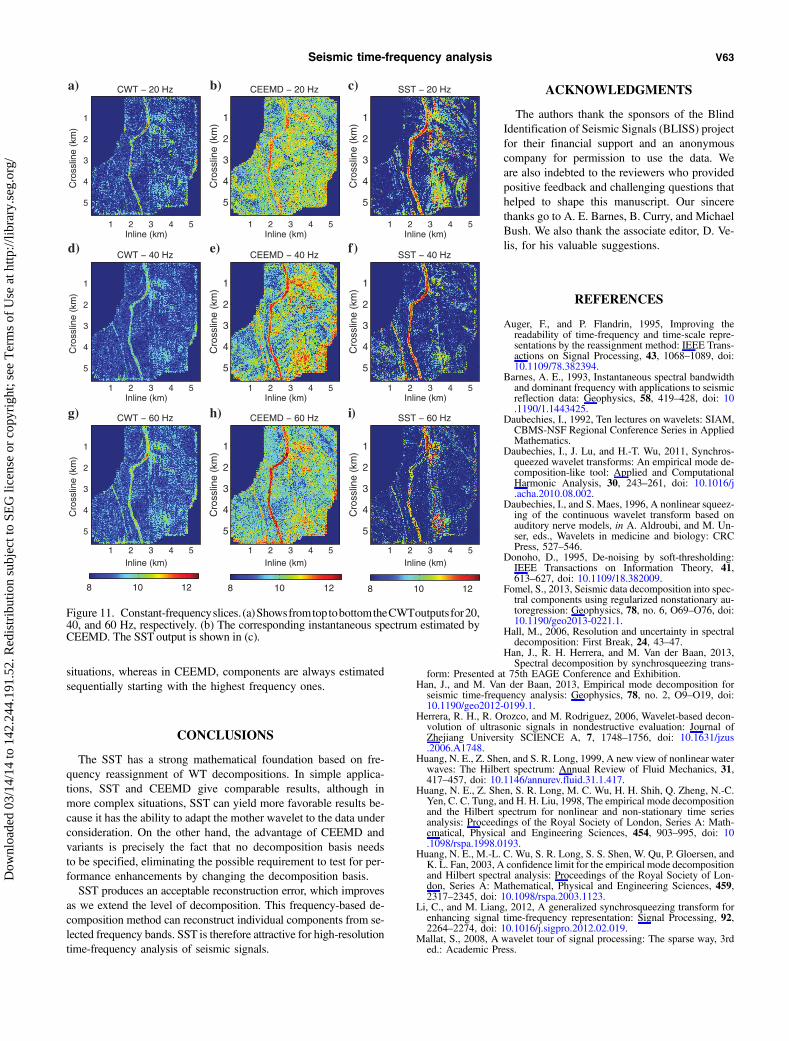
In our last test, we run the three algorithms on the entire seismiccube, composed of 225 inlines and 217 crosslines with a regularspacing of 25 m. Each trace is 450 samples long with a samplingperiod of 2 ms. Figure 10 shows the time slice at 420 ms of theseismic cube. Beside the channel, which is clearly shown through-out the image, there is a subtle fault. We compare the results ofCWT, CEEMD, and SST centered at this time slice analyzing differ-ent frequency slices. CWT and SST use a Morlet wavelet with 32levels per octave, and CEEMD injects 10% of Gaussian white noiseusing 50 realizations.Figure 11 shows the resulting constant frequency slices for CWT

(a), CEEMD (b), and SST (c) at, respectively, 20, 40, and 60 Hz (topto bottom). The channel and fault are more sharply represented byCEEMD and SST than in the CWT maps. CEEMD and SST havesimilar performance; however, only SST seems to show that the60 Hz spectral component is fading.The fault appears at the 40 and 60 Hz time slices of all three

methods. The CWT shows the main features on all three frequencyslices, yet their amplitude variations are less clear, which makes thethickness calculation of the channel challenging during further in-terpretation. Compared with CWT, the amplitude variation ofCEEMD and SSTalong the channel is better defined, which is help-ful to calculate subtle thickness variations. The amplitude variationsbetween closely spaced frequencies are better resolved in theCEEMD and SST result due to significantly reduced frequencysmearing and smaller spectral leakage than for the CWT and STFTmethods (Han et al., 2013). In addition, the CWT depicts a ratherhomogeneous area in the zone to the right of the channel in all fre-quency slices, whereas the CEEMD and SST results show more

variable magnitudes with areas of localized amplitude strengtheningand weakening plus several linear features.

DISCUSSION

SST can be used to accurately map time-domain signals into theirtime-frequency representation. It has a well-grounded mathematicalfoundation that facilitates theoretical analysis. Like the alternativetransform methods, it is a mathematically reversible function,thereby allowing for signal reconstruction, possibly after removalof specific components.CEEMD performs exceptionally well overcoming mode-mixing

problems. The reconstruction error is around machine precision(Torres et al., 2011). The computation of the instantaneous fre-quency from the isolated modes leads to a well-defined time-frequency representation. SST shares many of the advantages ofCEEMD in practice, with an acceptable reconstruction error. Thus,both methods are suitable to decompose a seismic trace into indi-vidual components with the advantage of frequency localization. Itmay also aid in noise-attenuation problems in which the signal andnoise correspond to different components, likewise, a recently pro-posed technique based on regularized nonstationary autoregression(Fomel, 2013). As in this paper, Fomel (2013) also suggests seismicdata compression and seismic data regularization as possible appli-cations for seismic data decomposition into spectral components.Both approaches aim to decompose seismic data into a sum of os-cillatory signals with smoothly varying frequencies and smoothlyvarying amplitudes (Fomel, 2013; Thakur et al., 2013), which isthe principle of the decomposition using the CWT (Daubechieset al., 2011).CEEMD using 50 noise realizations is approximately 13 times

slower than SST using our parameter settings; SST has approxi-mately the same cost as a WT, yet neither method is prohibitivelyexpensive. We found that by using a classical Morlet wavelet and 32levels for the SST method, we get a good balance between speedand resolution in the frequency representation. The improvement ofSST is clear compared with the CWT. The reassignment techniqueplays an important role in the results, by reallocating the waveletenergy to the corresponding time position.CEEMD and SST are more appropriate than STFT and CWT

when better time-frequency localization is needed. On the otherhand, STFT and CWT remain very useful analysis methods, evenif they may be subject to more spectral leakage than the CEEMDand SST methods, because they do not collapse spectra to narrowfrequency bands. For instance, many attenuation methods are basedon spectral ratios between two signals (Reine et al., 2009, 2012).Spectral ratios are difficult to compute if only individual frequencylines exist. On the other hand, it may be possible to use the fre-quency-shift method (Quan and Harris, 1997) to estimate seismicattenuation using the CEEMD and SST methods. SST, due to thereassignment step, will concentrate the energy into a small spectralband. Thus, it will be more appropriate when better time-frequencylocalization is needed (such as stratigraphic mapping to detect chan-nel structures or identification of resonance frequencies).From our study, we find that SST and CEEMD perform equally

well for seismic time-frequency representation, with the advantageof speed and a stronger mathematical foundation in the case of theSST. A further difference is that in the SST method, one can specifythe frequency range of interest prior to decomposition via the CWTscale parametrization. This can speed up computations in many

Inline (m)

Cro

sslin

e (m

)

Amplitude

1000 2000 3000 4000 5000

500

1000

1500

2000

2500

3000

3500

4000

4500

5000

5500 −3

−2

−1

0

1

2

3x 10

6

Channel

Fault

Channel

Fault

Figure 10. Time slice at 420 ms. The channel and fault are clearlyvisible. The vertical white line, at inline 2050 m, represents the sec-tion displayed in Figure 6.

V62 Herrera et al.

Dow

nloa

ded

03/1

4/14

to 1

42.2

44.1

91.5

2. R

edis

trib

utio

n su

bjec

t to

SEG

lice

nse

or c

opyr

ight

; see

Ter

ms

of U

se a

t http

://lib

rary

.seg

.org

/

situations, whereas in CEEMD, components are always estimatedsequentially starting with the highest frequency ones.

CONCLUSIONS

The SST has a strong mathematical foundation based on fre-quency reassignment of WT decompositions. In simple applica-tions, SST and CEEMD give comparable results, although inmore complex situations, SST can yield more favorable results be-cause it has the ability to adapt the mother wavelet to the data underconsideration. On the other hand, the advantage of CEEMD andvariants is precisely the fact that no decomposition basis needsto be specified, eliminating the possible requirement to test for per-formance enhancements by changing the decomposition basis.SST produces an acceptable reconstruction error, which improves

as we extend the level of decomposition. This frequency-based de-composition method can reconstruct individual components from se-lected frequency bands. SST is therefore attractive for high-resolutiontime-frequency analysis of seismic signals.

ACKNOWLEDGMENTS

The authors thank the sponsors of the BlindIdentification of Seismic Signals (BLISS) projectfor their financial support and an anonymouscompany for permission to use the data. Weare also indebted to the reviewers who providedpositive feedback and challenging questions thathelped to shape this manuscript. Our sincerethanks go to A. E. Barnes, B. Curry, and MichaelBush. We also thank the associate editor, D. Ve-lis, for his valuable suggestions.

REFERENCES

Auger, F., and P. Flandrin, 1995, Improving thereadability of time-frequency and time-scale repre-sentations by the reassignment method: IEEE Trans-actions on Signal Processing, 43, 1068–1089, doi:10.1109/78.382394.

Barnes, A. E., 1993, Instantaneous spectral bandwidthand dominant frequency with applications to seismicreflection data: Geophysics, 58, 419–428, doi: 10.1190/1.1443425.

Daubechies, I., 1992, Ten lectures on wavelets: SIAM,CBMS-NSF Regional Conference Series in AppliedMathematics.

Daubechies, I., J. Lu, and H.-T. Wu, 2011, Synchros-queezed wavelet transforms: An empirical mode de-composition-like tool: Applied and ComputationalHarmonic Analysis, 30, 243–261, doi: 10.1016/j.acha.2010.08.002.

Daubechies, I., and S. Maes, 1996, A nonlinear squeez-ing of the continuous wavelet transform based onauditory nerve models, in A. Aldroubi, and M. Un-ser, eds., Wavelets in medicine and biology: CRCPress, 527–546.

Donoho, D., 1995, De-noising by soft-thresholding:IEEE Transactions on Information Theory, 41,613–627, doi: 10.1109/18.382009.

Fomel, S., 2013, Seismic data decomposition into spec-tral components using regularized nonstationary au-toregression: Geophysics, 78, no. 6, O69–O76, doi:10.1190/geo2013-0221.1.

Hall, M., 2006, Resolution and uncertainty in spectraldecomposition: First Break, 24, 43–47.

Han, J., R. H. Herrera, and M. Van der Baan, 2013,Spectral decomposition by synchrosqueezing trans-

form: Presented at 75th EAGE Conference and Exhibition.Han, J., and M. Van der Baan, 2013, Empirical mode decomposition forseismic time-frequency analysis: Geophysics, 78, no. 2, O9–O19, doi:10.1190/geo2012-0199.1.

Herrera, R. H., R. Orozco, and M. Rodriguez, 2006, Wavelet-based decon-volution of ultrasonic signals in nondestructive evaluation: Journal ofZhejiang University SCIENCE A, 7, 1748–1756, doi: 10.1631/jzus.2006.A1748.

Huang, N. E., Z. Shen, and S. R. Long, 1999, A new view of nonlinear waterwaves: The Hilbert spectrum: Annual Review of Fluid Mechanics, 31,417–457, doi: 10.1146/annurev.fluid.31.1.417.

Huang, N. E., Z. Shen, S. R. Long, M. C. Wu, H. H. Shih, Q. Zheng, N.-C.Yen, C. C. Tung, and H. H. Liu, 1998, The empirical mode decompositionand the Hilbert spectrum for nonlinear and non-stationary time seriesanalysis: Proceedings of the Royal Society of London, Series A: Math-ematical, Physical and Engineering Sciences, 454, 903–995, doi: 10.1098/rspa.1998.0193.

Huang, N. E., M.-L. C. Wu, S. R. Long, S. S. Shen, W. Qu, P. Gloersen, andK. L. Fan, 2003, A confidence limit for the empirical mode decompositionand Hilbert spectral analysis: Proceedings of the Royal Society of Lon-don, Series A: Mathematical, Physical and Engineering Sciences, 459,2317–2345, doi: 10.1098/rspa.2003.1123.

Li, C., and M. Liang, 2012, A generalized synchrosqueezing transform forenhancing signal time-frequency representation: Signal Processing, 92,2264–2274, doi: 10.1016/j.sigpro.2012.02.019.

Mallat, S., 2008, A wavelet tour of signal processing: The sparse way, 3rded.: Academic Press.

Inline (km)

Cro

sslin

e (k

m)

CWT − 20 Hz

1 2 3 4 5

1

a) b) c)

d) e) f)

g) h) i)

2

3

4

5

Inline (km)

Cro

sslin

e (k

m)

CEEMD − 20 Hz

1 2 3 4 5

1

2

3

4

5

Inline (km)

Cro

sslin

e (k

m)

SST − 20 Hz

1 2 3 4 5

1

2

3

4

5

Inline (km)

Cro

sslin

e (k

m)

CWT − 40 Hz

1 2 3 4 5

1

2

3

4

5

Inline (km)

Cro

sslin

e (k

m)

CEEMD − 40 Hz

1 2 3 4 5

1

2

3

4

5

Inline (km)

Cro

sslin

e (k

m)

SST − 40 Hz

1 2 3 4 5

1

2

3

4

5

Inline (km)

Cro

sslin

e (k

m)

CWT − 60 Hz

1 2 3 4 5

1

2

3

4

5

8 10 12

Inline (km)

Cro

sslin

e (k

m)

CEEMD − 60 Hz

1 2 3 4 5

1

2

3

4

5

8 10 12

Inline (km)

Cro

sslin

e (k

m)

SST − 60 Hz

1 2 3 4 5

1

2

3

4

5

8 10 12

Figure 11. Constant-frequencyslices. (a)ShowsfromtoptobottomtheCWToutputsfor20,40, and 60 Hz, respectively. (b) The corresponding instantaneous spectrum estimated byCEEMD. The SST output is shown in (c).

Seismic time-frequency analysis V63

Dow

nloa

ded

03/1

4/14

to 1

42.2

44.1

91.5

2. R

edis

trib

utio

n su

bjec

t to

SEG

lice

nse

or c

opyr

ight

; see

Ter

ms

of U

se a

t http

://lib

rary

.seg

.org

/

Meignen, S., T. Oberlin, and S. McLaughlin, 2012, A new algorithm formulticomponent signals analysis based on synchrosqueezing: With an ap-plication to signal sampling and denoising: IEEE Transactions on SignalProcessing, 60, 5787–5798, doi: 10.1109/TSP.2012.2212891.

Partyka, G., J. Gridley, and J. Lopez, 1999, Interpretational applications ofspectral decomposition in reservoir characterization: The Leading Edge,18, 353–360, doi: 10.1190/1.1438295.

Perz, M., 2001, Coals and their confounding effects: CSEG Recorder, 26,no. 12, 34–53.

Quan, Y., and J. M. Harris, 1997, Seismic attenuation tomography using thefrequency shift method: Geophysics, 62, 895–905, doi: 10.1190/1.1444197.

Reine, C., R. Clark, and M. van der Baan, 2012, Robust prestack Q-deter-mination using surface seismic data: Part 1 — Method and synthetic ex-amples: Geophysics, 77, no. 1, R45–R56, doi: 10.1190/geo2011-0073.1.

Reine, C., M. Van der Baan, and R. Clark, 2009, The robustness of seismicattenuation measurements using fixed- and variable-window time-frequency transforms: Geophysics, 74, no. 2, WA123–WA135, doi: 10.1190/1.3043726.

Thakur, G., E. Brevdo, N. S. Fučkar, and H.-T. Wu, 2013, The syn-chrosqueezing algorithm for time-varying spectral analysis: Robustnessproperties and new paleoclimate applications: Signal Processing, 93,1079–1094, doi: 10.1016/j.sigpro.2012.11.029.

Torres, M., M. Colominas, G. Schlotthauer, and P. Flandrin, 2011, A com-plete ensemble empirical mode decomposition with adaptive noise: IEEEInternational Conference on Acoustics, Speech and Signal Processing(ICASSP), 4144–4147, doi: 10.1109/ICASSP.2011.5947265.

Van der Baan, M., S. Fomel, and M. Perz, 2010, Nonstationary phase es-timation: A tool for seismic interpretation?: The Leading Edge, 29, 1020–1026, doi: 10.1190/1.3485762.

Wu, H.-T., P. Flandrin, and I. Daubechies, 2011, One or two frequencies?The synchrosqueezing answers: Advances in Adaptive Data Analysis, 3,no. 2, 29–39, doi: 10.1142/S179353691100074X.

Wu, Z., and N. E. Huang, 2009, Ensemble empirical mode decomposition: Anoise-assisted data analysis method: Advances in Adaptive Data Analysis,1, no. 1, 1–41, doi: 10.1142/S1793536909000047.

V64 Herrera et al.

Dow

nloa

ded

03/1

4/14

to 1

42.2

44.1

91.5

2. R

edis

trib

utio

n su

bjec

t to

SEG

lice

nse

or c

opyr

ight

; see

Ter

ms

of U

se a

t http

://lib

rary

.seg

.org

/