applications of renormalization group methods in nuclear ...ntg/talks/hugs_2014_furnstahl... ·...
TRANSCRIPT

Applications of Renormalization GroupMethods in Nuclear Physics – 6
Dick FurnstahlDepartment of PhysicsOhio State University
HUGS 2014

Outline: Lecture 6
Lecture 6: High-res. probes of low-res. nucleiRecap: Running HamiltoniansParton distributions as paradigmSummary and challengesExtra: High-res. probes of low-res. nuclei

Outline: Lecture 6
Lecture 6: High-res. probes of low-res. nucleiRecap: Running HamiltoniansParton distributions as paradigmSummary and challengesExtra: High-res. probes of low-res. nuclei

“Measuring” the QCD Hamiltonian: Running αs(Q2)
QCD α (Μ ) = 0.1184 ± 0.0007s Z
0.1
0.2
0.3
0.4
0.5
αs (Q)
1 10 100Q [GeV]
Heavy Quarkoniae+e– Annihilation
Deep Inelastic Scattering
July 2009
The QCD coupling is scaledependent (“running”):αs(Q2) ≈ [β0 ln(Q2/Λ2
QCD)]−1
The QCD coupling strength αs isscheme dependent (e.g., “V”scheme used on lattice, or MS)
Extractions from experiment canbe compared (here at MZ ):
0.11 0.12 0.13
α (Μ )s Z
Quarkonia (lattice)
DIS F2 (N3LO)
τ-decays (N3LO)
DIS jets (NLO)
e+e– jets & shps (NNLO)
electroweak fits (N3LO)
e+e– jets & shapes (NNLO)
Υ decays (NLO)
cf. QED, where αem(Q2) iseffectively constant for soft Q2:
αem(Q2 = 0) ≈ 1/137∴ fixed H for quantum chemistry

Running QCD αs(Q2) vs. running nuclear Vλ
QCD α (Μ ) = 0.1184 ± 0.0007s Z
0.1
0.2
0.3
0.4
0.5
αs (Q)
1 10 100Q [GeV]
Heavy Quarkoniae+e– Annihilation
Deep Inelastic Scattering
July 2009
The QCD coupling is scaledependent (cf. low-E QED):αs(Q2) ≈ [β0 ln(Q2/Λ2
QCD)]−1
The QCD coupling strength αsis scheme dependent (e.g., “V”scheme used on lattice, or MS)
Vary scale (“resolution”) with RG
Scale dependence: SRG (or Vlow k )running of initial potential with λ(decoupling or separation scale)
Scheme dependence: AV18 vs. N3LO(plus associated 3NFs)
But all are (NN) phase equivalent!
Shift contributions between interactionand sums over intermediate states

JLab: Understanding “short-range correlations” in nucleiCorrelations in nuclear systems
A!1A
q
A
q
e e
e’ e’
a) b)
A!2
N
NN
FIGURE 1. The simple goal of short-range nucleon-nucleon correlation studies is to cleanly isolate diagram b) from a).Unfortunately, there are many other diagrams, including those with final-state interactions, that can produce the same final state asthe diagram scientists would like to isolate. If one could find kinematics that were dominated by diagram b) it would finally allowelectron scattering to provide new insights into the short-range part of the nucleon-nucleon potential.
For A(e,e’p) reactions, one can determine not only the energy and moment transferred, but also the energy and
momentum of the knocked-out nucleon. The difference between the transferred and detected energy and momentum
is referred to as the missing energy, Emiss and missing momentum, pmiss, respectively. From the theoretical works on
how short-range nucleon-nucleon correlations effects the momentum distribution of nucleons in the nucleus [6], it
is clear one must probe beyond the simple particle in an average potential motion of the nucleon in the nucleus of
approximately 250 MeV/c in order to observe the effects of correlations.
With the construction of the Jefferson Lab Continuous Electron Beam Facility (CEBAF) [7], it was possible to
do high-luminosity knock-out reactions in ideal quasi-elastic kinematics into the pmiss > 250 MeV/c region. In the
early Jefferson Lab knock-out reaction proposals, such as E89-044 3He(e,e’p)pn and 3He(e,e’p)d, these kinematics
were argued as the key to cleanly observe the effects of short-range correlations. And while final results of the
experiments were clearly effected by the presence of correlations, the magnitude of the cross sections in the high
missing momentum region was dominated by final-state interaction effects [8, 9]. Equally striking was the D(e,e’p)n
data from CLAS taken at Q2 > 5 [GeV/c]2 in xB < 1 kinematics [10]. Here it was shown that meson-exchange currents,final-state interaction, and delta-isobar configurations mask cleanly probing nucleon-nucleons even at extremely high
Q2 in xB < 1 kinematics.
NUCLEAR SCALING
With both the xB < 1 and xB = 1 kinematics practically ruled out for ever being able to cleanly probe short-range
correlations; there is only one region left to explore: xB > 1. This is a special region, since it is kinematically
forbidden for a free nucleon, and thus seems to be a natural place to observe effects of multi-nucleon interactions.
These kinematics were probed with limited statistics at SLAC [11] and the plateaus in the per nucleon ratios, r(A/d),
were claimed at to be evidence for short-range correlations [12].
In 2003, CLAS published high statics data in the same kinematic region. The results clearly showed that the plateaus
could only be seen for Q2 > 1 [GeV/c]2 and xB > 1 kinematics [13] as predicted by Frankfurt and Strikman [14]. But
plateaus alone are not evidence for correlations, just evidence that the functional form of the cross section is the same
for the two nuclei; so data was taken the xB > 2 region. By logic, if 1< xB < 2 is a region of two-nucleon correlations,
then the xB > 2 region should be dominated by three-nucleon correlations. The CLAS Q2 > 1 and xB > 2 experiment
reported observing a second scaling plateau as shown in Fig. 2 [15]. Preliminary results of Hall C high precision data
have shown roughly the same magnitude for these plateaus as CLAS and shown that there is no Q2 dependence in the
2< Q2 < 4 [GeV/c]2 range [16, 17].
Subedi et al., Science 320, 1476 (2008)
would demonstrate the presence of 3-nucleon (3N) SRCand confirm the previous observation of NN SRC.
Note that: (i) Refs. [5,6] argue that the c.m. motion of theNN SRC may change the value of a2 (by up to 20% for56Fe) but not the scaling at xB < 2. For 3N SRC there areno estimates of the effects of c.m. motion. (ii) Final stateinteractions (FSI) are dominated by the interaction of thestruck nucleon with the other nucleons in the SRC [7,8].Hence the FSI can modify !j, while such modification ofaj!A" are small since the pp, pn, and nn cross sections atQ2 > 1 GeV2 are similar in magnitudes.
In our previous work [6] we showed that the ratiosR!A; 3He" # 3!A!Q2;xB"
A!3He!Q2;xB" scale for 1:5< xB < 2 and 1:4<
Q2 < 2:6 GeV2, confirming findings in Ref. [7]. Here werepeat our previous measurement with higher statisticswhich allows us to estimate the absolute per-nucleon prob-abilities of NN SRC.
We also search for the even more elusive 3N SRC,correlations which originate from both short-range NNinteractions and three-nucleon forces, using the ratioR!A; 3He" at 2< xB $ 3.
Two sets of measurements were performed at theThomas Jefferson National Accelerator Facility in 1999and 2002. The 1999 measurements used 4.461 GeV elec-trons incident on liquid 3He, 4He and solid 12C targets. The2002 measurements used 4.471 GeVelectrons incident on asolid 56Fe target and 4.703 GeV electrons incident on aliquid 3He target.
Scattered electrons were detected in the CLAS spec-trometer [9]. The lead-scintillator electromagnetic calo-rimeter provided the electron trigger and was used toidentify electrons in the analysis. Vertex cuts were usedto eliminate the target walls. The estimated remainingcontribution from the two Al 15 "m target cell windowsis less than 0.1%. Software fiducial cuts were used toexclude regions of nonuniform detector response. Kine-matic corrections were applied to compensate for driftchamber misalignments and magnetic field uncertainties.
We used the GEANT-based CLAS simulation, GSIM, todetermine the electron acceptance correction factors, tak-ing into account ‘‘bad’’ or ‘‘dead’’ hardware channels invarious components of CLAS. The measured acceptance-corrected, normalized inclusive electron yields on 3He,4He, 12C, and 56Fe at 1< xB < 2 agree with Sargsian’sradiated cross sections [10] that were tuned on SLAC data[11] and describe reasonably well the Jefferson Lab Hall C[12] data.
We constructed the ratios of inclusive cross sections as afunction of Q2 and xB, with corrections for the CLASacceptance and for the elementary electron-nucleon crosssections:
r!A; 3He" # A!2!ep % !en"3!Z!ep % N!en"
3Y!A"AY!3He"R
Arad; (2)
where Z and N are the number of protons and neutrons innucleus A, !eN is the electron-nucleon cross section, Y isthe normalized yield in a given (Q2; xB) bin, and RA
rad is theratio of the radiative correction factors for 3He and nucleusA [see Ref. [8] ]. In our Q2 range, the elementary crosssection correction factor A!2!ep%!en"
3!Z!ep%N!en" is 1:14& 0:02 for C
and 4He and 1:18& 0:02 for 56Fe. Note that the 3He yieldin Eq. (2) is also corrected for the beam energy differenceby the difference in the Mott cross sections. The corrected3He cross sections at the two energies agree within $ 3:5%[8].
We calculated the radiative correction factors for thereaction A!e; e0" at xB < 2 using Sargsian’s upgradedcode of Ref. [13] and the formalism of Mo and Tsai [14].These factors change 10%–15% with xB for 1< xB < 2.However, their ratios, RA
rad, for 3He to the other nuclei arealmost constant (within 2%–3%) for xB > 1:4. We appliedRArad in Eq. (2) event by event for 0:8< xB < 2. Since there
are no theoretical cross section calculations at xB > 2, weapplied the value of RA
rad averaged over 1:4< xB < 2 to theentire 2< xB < 3 range. Since the xB dependence of RA
radfor 4He and 12C are very small, this should not affect theratio r of Eq. (2). For 56Fe, due to the observed small slopeof RA
rad with xB, r!A; 3He" can increase up to 4% at xB #2:55. This was included in the systematic errors.
Figure 1 shows the resulting ratios integrated over 1:4<Q2 < 2:6 GeV2. These cross section ratios (a) scale ini-tially for 1:5< xB < 2, which indicates that NN SRCs
a)
r(4 H
e/3 H
e)
b)
r(12
C/3 H
e)
xB
r(56
Fe/3 H
e)
c)
1
1.5
2
2.5
3
1
2
3
4
2
4
6
1 1.25 1.5 1.75 2 2.25 2.5 2.75
FIG. 1. Weighted cross section ratios [see Eq. (2)] of (a) 4He,(b) 12C, and (c) 56Fe to 3He as a function of xB for Q2 >1:4 GeV2. The horizontal dashed lines indicate the NN (1:5<xB < 2) and 3N (xB > 2:25) scaling regions.
PRL 96, 082501 (2006) P H Y S I C A L R E V I E W L E T T E R S week ending3 MARCH 2006
082501-3
Higinbotham, arXiv:1010.4433
Egiyan et al. PRL 96, 1082501 (2006)
What is this vertex?
k k� q = k − k�
ν = Ek − Ek�
p1
p2
p�1
SRC interpretation:
NN interaction can scatter states withto intermediate states with which are knocked out by the photon
p1, p2 � kF
How to explain cross sections in terms of low-momentum interactions?
Vertex depends on the resolution!
q
p�1
p�2
p�1, p�2 � kF
p�2
1.4 < Q2 < 2.6 GeV 2
Q2 = −q2
xB =Q2
2mNν
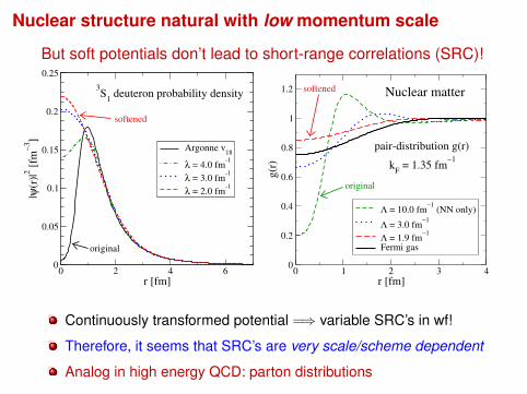
Nuclear structure natural with low momentum scale
But soft potentials don’t lead to short-range correlations (SRC)!
0 2 4 6r [fm]
0
0.05
0.1
0.15
0.2
0.25
|ψ(r
)|2 [
fm−
3]
Argonne v18
λ = 4.0 fm-1
λ = 3.0 fm-1
λ = 2.0 fm-1
3S
1 deuteron probability density
softened
original
0 1 2 3 4r [fm]
0
0.2
0.4
0.6
0.8
1
1.2
g(r
)
Λ = 10.0 fm−1
(NN only)
Λ = 3.0 fm−1
Λ = 1.9 fm−1
Fermi gas
pair-distribution g(r)
kF = 1.35 fm
−1
original
softened Nuclear matter
Continuously transformed potential =⇒ variable SRC’s in wf!
Therefore, it seems that SRC’s are very scale/scheme dependent
Analog in high energy QCD: parton distributions

Outline: Lecture 6
Lecture 6: High-res. probes of low-res. nucleiRecap: Running HamiltoniansParton distributions as paradigmSummary and challengesExtra: High-res. probes of low-res. nuclei

Parton distributions as paradigm [C. Keppel]
DIS Kinematics • Four-momentum transfer:
• Mott Cross Section (c=1):
22
2'
2
22
sin'4
)cos|'| ||'(2
)'()'()'(
QEEkkEEmm
kkkkEEq
ee
−≡−≈
=−−+=
=−⋅−−−=
2θ
θ
sorhadron ten :
sorlepton ten :
µν
µν
WL
)sin2(11
sin4
cos
)cos1(112
sin'16'4
'2'4
22
2422
22
2422
22
4
22
cos
cos)(
θθ
θ
θ
α
θθα
θασ
ME
ME
E
EEE
EE
QE
Mottdd
+
−+2
2Ω
⋅=
⋅=
⋅=
Electron scattering of a spinless point particle
a virtual photon of four-momentum q is able to resolve structures of the order /√q2
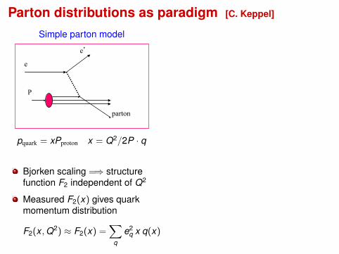
Parton distributions as paradigm [C. Keppel]
Simple parton model
e
P
parton
e�
pquark = xPproton x = Q2/2P · q
Bjorken scaling =⇒ structurefunction F2 independent of Q2
Measured F2(x) gives quarkmomentum distribution
F2(x ,Q2) ≈ F2(x) =∑
q
e2q x q(x)

Parton distributions as paradigm [C. Keppel]
Simple parton model
e
P
parton
e�
pquark = xPproton x = Q2/2P · q
Bjorken scaling =⇒ structurefunction F2 independent of Q2
Measured F2(x) gives quarkmomentum distribution
F2(x ,Q2) ≈ F2(x) =∑
q
e2q x q(x)

Parton distributions as paradigm [C. Keppel]
Higher the resolution(i.e. higher the Q2)more low x partons we“see”.
So what do we expect F2 as a function of x ata fixed Q2 to look like?
F2

Parton distributions as paradigm [C. Keppel]
1/3
1/3
1/3
F2(x)
F2(x)
F2(x)
x
x
x
Three quarkswith 1/3 oftotalprotonmomentum each.
Three quarkswith somemomentumsmearing.
The three quarksradiate partons at low x.
….The answer depends on the Q2!

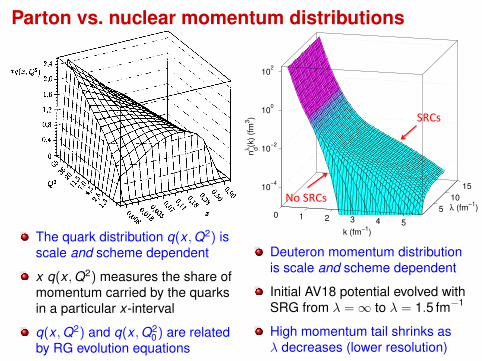
Parton vs. nuclear momentum distributions
The quark distribution q(x ,Q2) isscale and scheme dependent
x q(x ,Q2) measures the share ofmomentum carried by the quarksin a particular x-interval
q(x ,Q2) and q(x ,Q20) are related
by RG evolution equations
0 1 2 3 4 5
5
10
1510!4
10!2
100
102
! (fm!1)
k (fm!1)
nd!(k
) (f
m3) SRCs%
No%SRCs%
Deuteron momentum distributionis scale and scheme dependent
Initial AV18 potential evolved withSRG from λ =∞ to λ = 1.5 fm−1
High momentum tail shrinks asλ decreases (lower resolution)

Factorization: high-E QCD vs. low-E nuclear
Parton distributions as paradigm [Marco Stratman]
July, 25-28 2005 PHENIX Spin Fest @ RIKEN Wako 20
!"#$%&'("$'%)*+#,-.-+
!"#$%&"'()&*!&*+*,$'$"%,)%-)-'#$%&".'$"%,/
,"&/*+#"0-
1"#$%&'("$'%)
-232
42*#0%"#*)%-) -5*/-1')-+*6%&/-&0')-*6-$7--)*0%)389+,%&$8/'+$")#-
:2*#0%"#*)%-)+#0*1*5*&-8+,;110')3*1')'$-*<'-#-+*
$,-*+-<"&"$'%) 6-$7--)*0%)38 ")/*+,%&$8/'+$")#-*<,=+'#+*'+*)%$*;)'>;-
+,%&$8/'+$")#-?'0+%)*#%-11'#'-)$
0%)38/'+$")#-<"&$%)*/-)+'$=
F2(x ,Q2) ∼∑a fa(x , µf )⊗ F a
2 (x ,Q/µf )
Parton distributions as paradigm [Marco Stratman]
July, 25-28 2005 PHENIX Spin Fest @ RIKEN Wako 20
!"#$%&'("$'%)*+#,-.-+
!"#$%&"'()&*!&*+*,$'$"%,)%-)-'#$%&".'$"%,/
,"&/*+#"0-
1"#$%&'("$'%)
-232
42*#0%"#*)%-) -5*/-1')-+*6%&/-&0')-*6-$7--)*0%)389+,%&$8/'+$")#-
:2*#0%"#*)%-)+#0*1*5*&-8+,;110')3*1')'$-*<'-#-+*
$,-*+-<"&"$'%) 6-$7--)*0%)38 ")/*+,%&$8/'+$")#-*<,=+'#+*'+*)%$*;)'>;-
+,%&$8/'+$")#-?'0+%)*#%-11'#'-)$
0%)38/'+$")#-<"&$%)*/-)+'$= ↔
Parton distributions as paradigm [Marco Stratman]
July, 25-28 2005 PHENIX Spin Fest @ RIKEN Wako 20
!"#$%&'("$'%)*+#,-.-+
!"#$%&"'()&*!&*+*,$'$"%,)%-)-'#$%&".'$"%,/
,"&/*+#"0-
1"#$%&'("$'%)
-232
42*#0%"#*)%-) -5*/-1')-+*6%&/-&0')-*6-$7--)*0%)389+,%&$8/'+$")#-
:2*#0%"#*)%-)+#0*1*5*&-8+,;110')3*1')'$-*<'-#-+*
$,-*+-<"&"$'%) 6-$7--)*0%)38 ")/*+,%&$8/'+$")#-*<,=+'#+*'+*)%$*;)'>;-
+,%&$8/'+$")#-?'0+%)*#%-11'#'-)$
0%)38/'+$")#-<"&$%)*/-)+'$=
Separation between long- andshort-distance physics is notunique =⇒ introduce µf
Choice of µf defines borderbetween long/short distance
Form factor F2 is independentof µf , but pieces are not
Q2 running of fa(x ,Q2) comesfrom choosing µf to optimizeextraction from experiment
Also has factorization assumptions(e.g., from D. Bazin ECT* talk, 5/2011)
D. Bazin, Workshop on Recent Developments in Transfer and Knockout Reactions, May 9-13, 2011, Trento, Italy
Conundrum
• Using reactions to study nuclear structure
• One observable, two models
• To extract structure information, need accurate reaction model
!if
=
!
|Jf!Ji|"j"Jf +Ji
Sifj !sp
Observable: cross section
Structure model: spectroscopic factor
Reaction model: single-particlecross section
Is the factorization general/robust?(Process dependence?)
What does it mean to be consistentbetween structure and reactionmodels? Treat separately? (No!)
How does scale/schemedependence come in?
What are the trade-offs? (Doessimpler structure always meanmuch more complicated reaction?)

Scheming for parton distributionsNeed schemes for both renormalization and factorization
From the “Handbook of perturbative QCD” by G. Sterman et al.
“Short-distance finite parts at higher orders may beapportioned arbitrarily between the C’s and φ’s. A prescriptionthat eliminates this ambiguity is what we mean by afactorization scheme. . . . The two most commonly usedschemes, called DIS and MS, reflect two different uses towhich the freedom in factorization may be put.”
“The choice of scheme is a matter of taste and convenience,but it is absolutely crucial to use schemes consistently, and toknow in which scheme any given calculation, or comparison todata, is carried out.”
Specifying a scheme in low-energy nuclear physics includesspecifying a potential, including regulators, and how a reaction isanalyzed.

Standard story for (e,e′p) [from C. Ciofi degli Atti]
In IA: “missing” momentum pm = k1 and energy Em = E
Common assumption: FSI and two-body currents treatableas independent add-ons to impulse approximation
Is this valid?
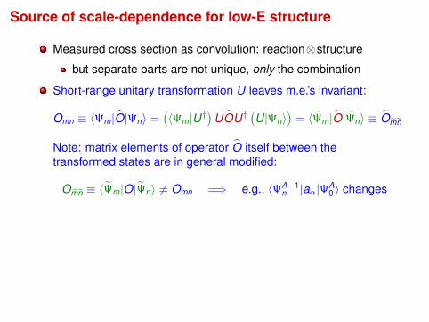
Source of scale-dependence for low-E structure
Measured cross section as convolution: reaction⊗structure
but separate parts are not unique, only the combination
Short-range unitary transformation U leaves m.e.’s invariant:
Omn ≡ 〈Ψm|O|Ψn〉 =(〈Ψm|U†
)UOU†
(U|Ψn〉
)= 〈Ψm|O|Ψn〉 ≡ Omn
Note: matrix elements of operator O itself between thetransformed states are in general modified:
Omn ≡ 〈Ψm|O|Ψn〉 6= Omn =⇒ e.g., 〈ΨA−1n |aα|ΨA
0 〉 changes
In a low-energy effective theory, transformations that modifyshort-range unresolved physics =⇒ equally valid states.So Omn 6= Omn =⇒ scale/scheme dependent observables.
RG unitary transformations change the decoupling scale =⇒change the factorization scale. Use to characterize and explorescale and scheme and process dependence!
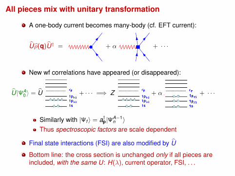
All pieces mix with unitary transformation
A one-body current becomes many-body (cf. EFT current):
Uρ(q)U† = + α + · · ·
New wf correlations have appeared (or disappeared):
U|ΨA0 〉 = U
12C(e, e!p)X
1966 1988 2006
+ · · · =⇒ Z
12C(e, e!p)X
1966 1988 2006
+ α
12C(e, e!p)X
1966 1988 2006
+ · · ·
Similarly with |Ψf 〉 = a†p|ΨA−1n 〉
Thus spectroscopic factors are scale dependent
Final state interactions (FSI) are also modified by U
Bottom line: the cross section is unchanged only if all pieces areincluded, with the same U: H(λ), current operator, FSI, . . .

How should one choose a scale and/or scheme?
To make calculations easier or more convergentQCD running coupling and scale: improved perturbationtheory; choosing a gauge: e.g., Coulomb or LorentzLow-k potential: improve many-body convergence,
or to make microscopic connection to shell model or . . .(Near-) local potential: quantum Monte Carlo methods work
Better interpretation or intuition =⇒ predictabilitySRC phenomenology?
Cleanest extraction from experimentCan one “optimize” validity of impulse approximation?Ideally extract at one scale, evolve to others using RG
Plan: use range of scales to test calculations and physicsFind (match) Hamiltonians and operators with EFTUse renormalization group to consistently relate scales andquantitatively probe ambiguities (e.g., in spectroscopic factors)

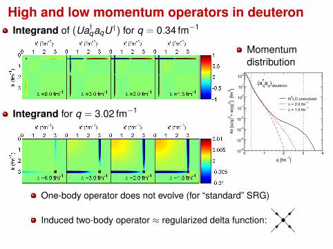
Operator flow in practice [e.g., see arXiv:1008.1569]
Evolution with s of anyoperator O is given by:
Os = UsOU†s
so Os evolves via
dOs
ds= [[Gs,Hs],Os]
Us =∑
i |ψi (s)〉〈ψi (0)|or solve dUs/ds flow
Matrix elements of evolvedoperators are unchanged
Consider momentumdistribution < ψd |a†qaq |ψd >
at q = 0.34 and 3.0 fm−1
in deuteron
0 1 2 3 4
q [fm−1]
10-5
10-4
10-3
10-2
10-1
100
101
102
4π [u
(q)2 +
w(q
)2 ] [fm
3 ]
N3LO unevolvedλ = 2.0 fm−1
λ = 1.5 fm−1
(a✝
qaq) deuteron
High and low momentum operators in deuteronIntegrand of (Ua†qaqU†) for q = 0.34 fm−1
Integrand for q = 3.02 fm−1
Momentumdistribution
0 1 2 3 4
q [fm−1]
10-5
10-4
10-3
10-2
10-1
100
101
102
4π [u
(q)2 +
w(q
)2 ] [fm
3 ]
N3LO unevolvedλ = 2.0 fm−1
λ = 1.5 fm−1
(a✝
qaq) deuteron
One-body operator does not evolve (for “standard” SRG)
Induced two-body operator ≈ regularized delta function:

High and low momentum operators in deuteronIntegrand of 〈ψd | (Ua†qaqU†) |ψd〉 for q = 0.34 fm−1
Integrand for q = 3.02 fm−1
Momentumdistribution
0 1 2 3 4
q [fm−1]
10-5
10-4
10-3
10-2
10-1
100
101
102
4π [u
(q)2 +
w(q
)2 ] [fm
3 ]
N3LO unevolvedλ = 2.0 fm−1
λ = 1.5 fm−1
(a✝
qaq) deuteron
Decoupling =⇒ High momentum components suppressed
Integrated value does not change, but nature of operator does
Similar for other operators:⟨r2⟩, 〈Qd 〉, 〈1/r〉
⟨ 1r
⟩, 〈GC〉, . . .

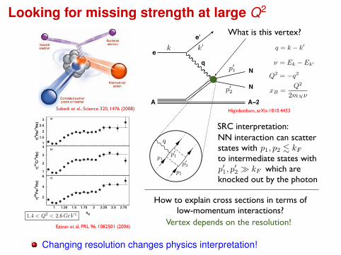
Looking for missing strength at large Q2Correlations in nuclear systems
A!1A
q
A
q
e e
e’ e’
a) b)
A!2
N
NN
FIGURE 1. The simple goal of short-range nucleon-nucleon correlation studies is to cleanly isolate diagram b) from a).Unfortunately, there are many other diagrams, including those with final-state interactions, that can produce the same final state asthe diagram scientists would like to isolate. If one could find kinematics that were dominated by diagram b) it would finally allowelectron scattering to provide new insights into the short-range part of the nucleon-nucleon potential.
For A(e,e’p) reactions, one can determine not only the energy and moment transferred, but also the energy and
momentum of the knocked-out nucleon. The difference between the transferred and detected energy and momentum
is referred to as the missing energy, Emiss and missing momentum, pmiss, respectively. From the theoretical works on
how short-range nucleon-nucleon correlations effects the momentum distribution of nucleons in the nucleus [6], it
is clear one must probe beyond the simple particle in an average potential motion of the nucleon in the nucleus of
approximately 250 MeV/c in order to observe the effects of correlations.
With the construction of the Jefferson Lab Continuous Electron Beam Facility (CEBAF) [7], it was possible to
do high-luminosity knock-out reactions in ideal quasi-elastic kinematics into the pmiss > 250 MeV/c region. In the
early Jefferson Lab knock-out reaction proposals, such as E89-044 3He(e,e’p)pn and 3He(e,e’p)d, these kinematics
were argued as the key to cleanly observe the effects of short-range correlations. And while final results of the
experiments were clearly effected by the presence of correlations, the magnitude of the cross sections in the high
missing momentum region was dominated by final-state interaction effects [8, 9]. Equally striking was the D(e,e’p)n
data from CLAS taken at Q2 > 5 [GeV/c]2 in xB < 1 kinematics [10]. Here it was shown that meson-exchange currents,final-state interaction, and delta-isobar configurations mask cleanly probing nucleon-nucleons even at extremely high
Q2 in xB < 1 kinematics.
NUCLEAR SCALING
With both the xB < 1 and xB = 1 kinematics practically ruled out for ever being able to cleanly probe short-range
correlations; there is only one region left to explore: xB > 1. This is a special region, since it is kinematically
forbidden for a free nucleon, and thus seems to be a natural place to observe effects of multi-nucleon interactions.
These kinematics were probed with limited statistics at SLAC [11] and the plateaus in the per nucleon ratios, r(A/d),
were claimed at to be evidence for short-range correlations [12].
In 2003, CLAS published high statics data in the same kinematic region. The results clearly showed that the plateaus
could only be seen for Q2 > 1 [GeV/c]2 and xB > 1 kinematics [13] as predicted by Frankfurt and Strikman [14]. But
plateaus alone are not evidence for correlations, just evidence that the functional form of the cross section is the same
for the two nuclei; so data was taken the xB > 2 region. By logic, if 1< xB < 2 is a region of two-nucleon correlations,
then the xB > 2 region should be dominated by three-nucleon correlations. The CLAS Q2 > 1 and xB > 2 experiment
reported observing a second scaling plateau as shown in Fig. 2 [15]. Preliminary results of Hall C high precision data
have shown roughly the same magnitude for these plateaus as CLAS and shown that there is no Q2 dependence in the
2< Q2 < 4 [GeV/c]2 range [16, 17].
Subedi et al., Science 320, 1476 (2008)
would demonstrate the presence of 3-nucleon (3N) SRCand confirm the previous observation of NN SRC.
Note that: (i) Refs. [5,6] argue that the c.m. motion of theNN SRC may change the value of a2 (by up to 20% for56Fe) but not the scaling at xB < 2. For 3N SRC there areno estimates of the effects of c.m. motion. (ii) Final stateinteractions (FSI) are dominated by the interaction of thestruck nucleon with the other nucleons in the SRC [7,8].Hence the FSI can modify !j, while such modification ofaj!A" are small since the pp, pn, and nn cross sections atQ2 > 1 GeV2 are similar in magnitudes.
In our previous work [6] we showed that the ratiosR!A; 3He" # 3!A!Q2;xB"
A!3He!Q2;xB" scale for 1:5< xB < 2 and 1:4<
Q2 < 2:6 GeV2, confirming findings in Ref. [7]. Here werepeat our previous measurement with higher statisticswhich allows us to estimate the absolute per-nucleon prob-abilities of NN SRC.
We also search for the even more elusive 3N SRC,correlations which originate from both short-range NNinteractions and three-nucleon forces, using the ratioR!A; 3He" at 2< xB $ 3.
Two sets of measurements were performed at theThomas Jefferson National Accelerator Facility in 1999and 2002. The 1999 measurements used 4.461 GeV elec-trons incident on liquid 3He, 4He and solid 12C targets. The2002 measurements used 4.471 GeVelectrons incident on asolid 56Fe target and 4.703 GeV electrons incident on aliquid 3He target.
Scattered electrons were detected in the CLAS spec-trometer [9]. The lead-scintillator electromagnetic calo-rimeter provided the electron trigger and was used toidentify electrons in the analysis. Vertex cuts were usedto eliminate the target walls. The estimated remainingcontribution from the two Al 15 "m target cell windowsis less than 0.1%. Software fiducial cuts were used toexclude regions of nonuniform detector response. Kine-matic corrections were applied to compensate for driftchamber misalignments and magnetic field uncertainties.
We used the GEANT-based CLAS simulation, GSIM, todetermine the electron acceptance correction factors, tak-ing into account ‘‘bad’’ or ‘‘dead’’ hardware channels invarious components of CLAS. The measured acceptance-corrected, normalized inclusive electron yields on 3He,4He, 12C, and 56Fe at 1< xB < 2 agree with Sargsian’sradiated cross sections [10] that were tuned on SLAC data[11] and describe reasonably well the Jefferson Lab Hall C[12] data.
We constructed the ratios of inclusive cross sections as afunction of Q2 and xB, with corrections for the CLASacceptance and for the elementary electron-nucleon crosssections:
r!A; 3He" # A!2!ep % !en"3!Z!ep % N!en"
3Y!A"AY!3He"R
Arad; (2)
where Z and N are the number of protons and neutrons innucleus A, !eN is the electron-nucleon cross section, Y isthe normalized yield in a given (Q2; xB) bin, and RA
rad is theratio of the radiative correction factors for 3He and nucleusA [see Ref. [8] ]. In our Q2 range, the elementary crosssection correction factor A!2!ep%!en"
3!Z!ep%N!en" is 1:14& 0:02 for C
and 4He and 1:18& 0:02 for 56Fe. Note that the 3He yieldin Eq. (2) is also corrected for the beam energy differenceby the difference in the Mott cross sections. The corrected3He cross sections at the two energies agree within $ 3:5%[8].
We calculated the radiative correction factors for thereaction A!e; e0" at xB < 2 using Sargsian’s upgradedcode of Ref. [13] and the formalism of Mo and Tsai [14].These factors change 10%–15% with xB for 1< xB < 2.However, their ratios, RA
rad, for 3He to the other nuclei arealmost constant (within 2%–3%) for xB > 1:4. We appliedRArad in Eq. (2) event by event for 0:8< xB < 2. Since there
are no theoretical cross section calculations at xB > 2, weapplied the value of RA
rad averaged over 1:4< xB < 2 to theentire 2< xB < 3 range. Since the xB dependence of RA
radfor 4He and 12C are very small, this should not affect theratio r of Eq. (2). For 56Fe, due to the observed small slopeof RA
rad with xB, r!A; 3He" can increase up to 4% at xB #2:55. This was included in the systematic errors.
Figure 1 shows the resulting ratios integrated over 1:4<Q2 < 2:6 GeV2. These cross section ratios (a) scale ini-tially for 1:5< xB < 2, which indicates that NN SRCs
a)
r(4 H
e/3 H
e)
b)
r(12
C/3 H
e)
xB
r(56
Fe/3 H
e)
c)
1
1.5
2
2.5
3
1
2
3
4
2
4
6
1 1.25 1.5 1.75 2 2.25 2.5 2.75
FIG. 1. Weighted cross section ratios [see Eq. (2)] of (a) 4He,(b) 12C, and (c) 56Fe to 3He as a function of xB for Q2 >1:4 GeV2. The horizontal dashed lines indicate the NN (1:5<xB < 2) and 3N (xB > 2:25) scaling regions.
PRL 96, 082501 (2006) P H Y S I C A L R E V I E W L E T T E R S week ending3 MARCH 2006
082501-3
Higinbotham, arXiv:1010.4433
Egiyan et al. PRL 96, 1082501 (2006)
What is this vertex?
k k� q = k − k�
ν = Ek − Ek�
p1
p2
p�1
SRC interpretation:
NN interaction can scatter states withto intermediate states with which are knocked out by the photon
p1, p2 � kF
How to explain cross sections in terms of low-momentum interactions?
Vertex depends on the resolution!
q
p�1
p�2
p�1, p�2 � kF
p�2
1.4 < Q2 < 2.6 GeV 2
Q2 = −q2
xB =Q2
2mNν
SRC explanation relies on high-momentum nucleons in structure!
Looking for missing strength at large Q2Correlations in nuclear systems
A!1A
q
A
q
e e
e’ e’
a) b)
A!2
N
NN
FIGURE 1. The simple goal of short-range nucleon-nucleon correlation studies is to cleanly isolate diagram b) from a).Unfortunately, there are many other diagrams, including those with final-state interactions, that can produce the same final state asthe diagram scientists would like to isolate. If one could find kinematics that were dominated by diagram b) it would finally allowelectron scattering to provide new insights into the short-range part of the nucleon-nucleon potential.
For A(e,e’p) reactions, one can determine not only the energy and moment transferred, but also the energy and
momentum of the knocked-out nucleon. The difference between the transferred and detected energy and momentum
is referred to as the missing energy, Emiss and missing momentum, pmiss, respectively. From the theoretical works on
how short-range nucleon-nucleon correlations effects the momentum distribution of nucleons in the nucleus [6], it
is clear one must probe beyond the simple particle in an average potential motion of the nucleon in the nucleus of
approximately 250 MeV/c in order to observe the effects of correlations.
With the construction of the Jefferson Lab Continuous Electron Beam Facility (CEBAF) [7], it was possible to
do high-luminosity knock-out reactions in ideal quasi-elastic kinematics into the pmiss > 250 MeV/c region. In the
early Jefferson Lab knock-out reaction proposals, such as E89-044 3He(e,e’p)pn and 3He(e,e’p)d, these kinematics
were argued as the key to cleanly observe the effects of short-range correlations. And while final results of the
experiments were clearly effected by the presence of correlations, the magnitude of the cross sections in the high
missing momentum region was dominated by final-state interaction effects [8, 9]. Equally striking was the D(e,e’p)n
data from CLAS taken at Q2 > 5 [GeV/c]2 in xB < 1 kinematics [10]. Here it was shown that meson-exchange currents,final-state interaction, and delta-isobar configurations mask cleanly probing nucleon-nucleons even at extremely high
Q2 in xB < 1 kinematics.
NUCLEAR SCALING
With both the xB < 1 and xB = 1 kinematics practically ruled out for ever being able to cleanly probe short-range
correlations; there is only one region left to explore: xB > 1. This is a special region, since it is kinematically
forbidden for a free nucleon, and thus seems to be a natural place to observe effects of multi-nucleon interactions.
These kinematics were probed with limited statistics at SLAC [11] and the plateaus in the per nucleon ratios, r(A/d),
were claimed at to be evidence for short-range correlations [12].
In 2003, CLAS published high statics data in the same kinematic region. The results clearly showed that the plateaus
could only be seen for Q2 > 1 [GeV/c]2 and xB > 1 kinematics [13] as predicted by Frankfurt and Strikman [14]. But
plateaus alone are not evidence for correlations, just evidence that the functional form of the cross section is the same
for the two nuclei; so data was taken the xB > 2 region. By logic, if 1< xB < 2 is a region of two-nucleon correlations,
then the xB > 2 region should be dominated by three-nucleon correlations. The CLAS Q2 > 1 and xB > 2 experiment
reported observing a second scaling plateau as shown in Fig. 2 [15]. Preliminary results of Hall C high precision data
have shown roughly the same magnitude for these plateaus as CLAS and shown that there is no Q2 dependence in the
2< Q2 < 4 [GeV/c]2 range [16, 17].
Subedi et al., Science 320, 1476 (2008)
would demonstrate the presence of 3-nucleon (3N) SRCand confirm the previous observation of NN SRC.
Note that: (i) Refs. [5,6] argue that the c.m. motion of theNN SRC may change the value of a2 (by up to 20% for56Fe) but not the scaling at xB < 2. For 3N SRC there areno estimates of the effects of c.m. motion. (ii) Final stateinteractions (FSI) are dominated by the interaction of thestruck nucleon with the other nucleons in the SRC [7,8].Hence the FSI can modify !j, while such modification ofaj!A" are small since the pp, pn, and nn cross sections atQ2 > 1 GeV2 are similar in magnitudes.
In our previous work [6] we showed that the ratiosR!A; 3He" # 3!A!Q2;xB"
A!3He!Q2;xB" scale for 1:5< xB < 2 and 1:4<
Q2 < 2:6 GeV2, confirming findings in Ref. [7]. Here werepeat our previous measurement with higher statisticswhich allows us to estimate the absolute per-nucleon prob-abilities of NN SRC.
We also search for the even more elusive 3N SRC,correlations which originate from both short-range NNinteractions and three-nucleon forces, using the ratioR!A; 3He" at 2< xB $ 3.
Two sets of measurements were performed at theThomas Jefferson National Accelerator Facility in 1999and 2002. The 1999 measurements used 4.461 GeV elec-trons incident on liquid 3He, 4He and solid 12C targets. The2002 measurements used 4.471 GeVelectrons incident on asolid 56Fe target and 4.703 GeV electrons incident on aliquid 3He target.
Scattered electrons were detected in the CLAS spec-trometer [9]. The lead-scintillator electromagnetic calo-rimeter provided the electron trigger and was used toidentify electrons in the analysis. Vertex cuts were usedto eliminate the target walls. The estimated remainingcontribution from the two Al 15 "m target cell windowsis less than 0.1%. Software fiducial cuts were used toexclude regions of nonuniform detector response. Kine-matic corrections were applied to compensate for driftchamber misalignments and magnetic field uncertainties.
We used the GEANT-based CLAS simulation, GSIM, todetermine the electron acceptance correction factors, tak-ing into account ‘‘bad’’ or ‘‘dead’’ hardware channels invarious components of CLAS. The measured acceptance-corrected, normalized inclusive electron yields on 3He,4He, 12C, and 56Fe at 1< xB < 2 agree with Sargsian’sradiated cross sections [10] that were tuned on SLAC data[11] and describe reasonably well the Jefferson Lab Hall C[12] data.
We constructed the ratios of inclusive cross sections as afunction of Q2 and xB, with corrections for the CLASacceptance and for the elementary electron-nucleon crosssections:
r!A; 3He" # A!2!ep % !en"3!Z!ep % N!en"
3Y!A"AY!3He"R
Arad; (2)
where Z and N are the number of protons and neutrons innucleus A, !eN is the electron-nucleon cross section, Y isthe normalized yield in a given (Q2; xB) bin, and RA
rad is theratio of the radiative correction factors for 3He and nucleusA [see Ref. [8] ]. In our Q2 range, the elementary crosssection correction factor A!2!ep%!en"
3!Z!ep%N!en" is 1:14& 0:02 for C
and 4He and 1:18& 0:02 for 56Fe. Note that the 3He yieldin Eq. (2) is also corrected for the beam energy differenceby the difference in the Mott cross sections. The corrected3He cross sections at the two energies agree within $ 3:5%[8].
We calculated the radiative correction factors for thereaction A!e; e0" at xB < 2 using Sargsian’s upgradedcode of Ref. [13] and the formalism of Mo and Tsai [14].These factors change 10%–15% with xB for 1< xB < 2.However, their ratios, RA
rad, for 3He to the other nuclei arealmost constant (within 2%–3%) for xB > 1:4. We appliedRArad in Eq. (2) event by event for 0:8< xB < 2. Since there
are no theoretical cross section calculations at xB > 2, weapplied the value of RA
rad averaged over 1:4< xB < 2 to theentire 2< xB < 3 range. Since the xB dependence of RA
radfor 4He and 12C are very small, this should not affect theratio r of Eq. (2). For 56Fe, due to the observed small slopeof RA
rad with xB, r!A; 3He" can increase up to 4% at xB #2:55. This was included in the systematic errors.
Figure 1 shows the resulting ratios integrated over 1:4<Q2 < 2:6 GeV2. These cross section ratios (a) scale ini-tially for 1:5< xB < 2, which indicates that NN SRCs
a)
r(4 H
e/3 H
e)
b)
r(12
C/3 H
e)
xB
r(56
Fe/3 H
e)
c)
1
1.5
2
2.5
3
1
2
3
4
2
4
6
1 1.25 1.5 1.75 2 2.25 2.5 2.75
FIG. 1. Weighted cross section ratios [see Eq. (2)] of (a) 4He,(b) 12C, and (c) 56Fe to 3He as a function of xB for Q2 >1:4 GeV2. The horizontal dashed lines indicate the NN (1:5<xB < 2) and 3N (xB > 2:25) scaling regions.
PRL 96, 082501 (2006) P H Y S I C A L R E V I E W L E T T E R S week ending3 MARCH 2006
082501-3
Higinbotham, arXiv:1010.4433
Egiyan et al. PRL 96, 1082501 (2006)
What is this vertex?
k k� q = k − k�
ν = Ek − Ek�
p1
p2
p�1
SRC interpretation:
NN interaction can scatter states withto intermediate states with which are knocked out by the photon
p1, p2 � kF
How to explain cross sections in terms of low-momentum interactions?
Vertex depends on the resolution!
q
p�1
p�2
p�1, p�2 � kF
p�2
1.4 < Q2 < 2.6 GeV 2
Q2 = −q2
xB =Q2
2mNν
Changing resolution changes physics interpretation!

Changing the separation scale with RG evolutionConventional analysis has (implied) high momentum scale
Based on potentials like AV18 and one-body current operator
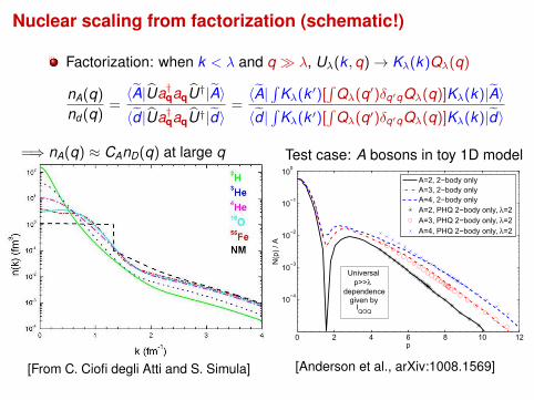
nA(k) � CA nD(k)
0 1 2 3 4
k [fm−1
]
10−5
10−4
10−3
10−2
10−1
100
101
102
n(k
) [
fm3]
AV18
Vsrg at λ = 2 fm−1
Vsrg at λ = 1.5 fm−1
CD-Bonn
N3LO (500 MeV)
[From C. Ciofi degli Atti and S. Simula]
With RG evolution, probability of high momentum decreases, but
n(k) ≡ 〈A|a†kak|A〉 =(〈A|U†
)Ua†kakU†
(U|Ψn〉
)= 〈A|Ua†kakU†|A〉
is unchanged! |A〉 is easier to calculate, but is operator too hard?

Nuclear scaling from factorization (schematic!)
Factorization: when k < λ and q � λ, Uλ(k ,q)→ Kλ(k)Qλ(q)
nA(q)
nd (q)=〈A|Ua†qaqU†|A〉〈d |Ua†qaqU†|d〉
=〈A|∫
Uλ(k ′,q′)δq′qU†λ(q, k)|A〉〈d |∫
Uλ(k ′,q′)δq′qU†λ(q, k)|d〉
=⇒ nA(q) ≈ CAnD(q) at large q
nA(k) � CA nD(k)
[From C. Ciofi degli Atti and S. Simula]
Test case: A bosons in toy 1D model
0 2 4 6 8 10 12
10−4
10−3
10−2
10−1
100
p
N(p
) / A
A=2, 2−body onlyA=3, 2−body onlyA=4, 2−body onlyA=2, PHQ 2−body only, λ=2A=3, PHQ 2−body only, λ=2A=4, PHQ 2−body only, λ=2
Universal p>>λdependence given by I
QOQ
[Anderson et al., arXiv:1008.1569]
Nuclear scaling from factorization (schematic!)
Factorization: when k < λ and q � λ, Uλ(k ,q)→ Kλ(k)Qλ(q)
nA(q)
nd (q)=〈A|Ua†qaqU†|A〉〈d |Ua†qaqU†|d〉
=〈A|∫
Kλ(k ′)[∫
Qλ(q′)δq′qQλ(q)]Kλ(k)|A〉〈d |∫
Kλ(k ′)[∫
Qλ(q′)δq′qQλ(q)]Kλ(k)|d〉
=⇒ nA(q) ≈ CAnD(q) at large q
nA(k) � CA nD(k)
[From C. Ciofi degli Atti and S. Simula]
Test case: A bosons in toy 1D model
0 2 4 6 8 10 12
10−4
10−3
10−2
10−1
100
p
N(p
) / A
A=2, 2−body onlyA=3, 2−body onlyA=4, 2−body onlyA=2, PHQ 2−body only, λ=2A=3, PHQ 2−body only, λ=2A=4, PHQ 2−body only, λ=2
Universal p>>λdependence given by I
QOQ
[Anderson et al., arXiv:1008.1569]

Nuclear scaling from factorization (schematic!)
Factorization: when k < λ and q � λ, Uλ(k ,q)→ Kλ(k)Qλ(q)
nA(q)
nd (q)=〈A|Ua†qaqU†|A〉〈d |Ua†qaqU†|d〉
=〈A|∫
Kλ(k ′)Kλ(k)|A〉〈d |∫
Kλ(k ′)Kλ(k)|d〉≡ CA
=⇒ nA(q) ≈ CAnD(q) at large q
nA(k) � CA nD(k)
[From C. Ciofi degli Atti and S. Simula]
Test case: A bosons in toy 1D model
0 2 4 6 8 10 12
10−4
10−3
10−2
10−1
100
p
N(p
) / A
A=2, 2−body onlyA=3, 2−body onlyA=4, 2−body onlyA=2, PHQ 2−body only, λ=2A=3, PHQ 2−body only, λ=2A=4, PHQ 2−body only, λ=2
Universal p>>λdependence given by I
QOQ
[Anderson et al., arXiv:1008.1569]

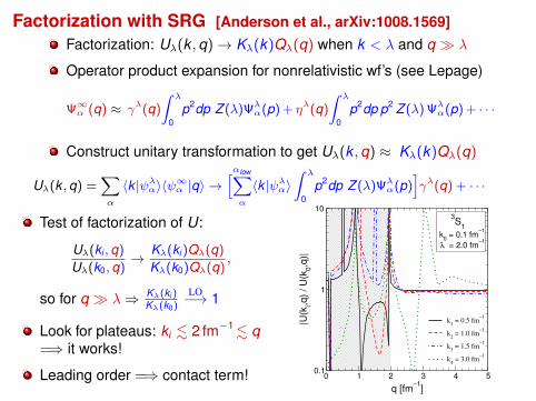
Factorization with SRG [Anderson et al., arXiv:1008.1569]Factorization: Uλ(k ,q)→ Kλ(k)Qλ(q) when k < λ and q � λ
Operator product expansion for nonrelativistic wf’s (see Lepage)
Ψ∞α (q) ≈ γλ(q)
∫ λ
0p2dp Z (λ)Ψλ
α(p) + ηλ(q)
∫ λ
0p2dp p2 Z (λ) Ψλ
α(p) + · · ·
Construct unitary transformation to get Uλ(k ,q) ≈ Kλ(k)Qλ(q)
Uλ(k , q) =∑α
〈k |ψλα〉〈ψ∞α |q〉 →
[αlow∑α
〈k |ψλα〉∫ λ
0p2dp Z (λ)Ψλ
α(p)]γλ(q) + · · ·
Test of factorization of U:
Uλ(ki , q)
Uλ(k0, q)→ Kλ(ki )Qλ(q)
Kλ(k0)Qλ(q),
so for q � λ⇒ Kλ(ki )Kλ(k0)
LO−→ 1
Look for plateaus: ki . 2 fm−1. q=⇒ it works!
Leading order =⇒ contact term! 0 1 2 3 4 5
q [fm−1
]
0.1
1
10
|U(k
i,q)
/ U
(k0,q
)|
k1 = 0.5 fm
−1
k2 = 1.0 fm
−1
k3 = 1.5 fm
−1
k4 = 3.0 fm
−1
λ = 2.0 fm−1
1S
0
k0 = 0.1 fm
−1
Factorization with SRG [Anderson et al., arXiv:1008.1569]Factorization: Uλ(k ,q)→ Kλ(k)Qλ(q) when k < λ and q � λ
Operator product expansion for nonrelativistic wf’s (see Lepage)
Ψ∞α (q) ≈ γλ(q)
∫ λ
0p2dp Z (λ)Ψλ
α(p) + ηλ(q)
∫ λ
0p2dp p2 Z (λ) Ψλ
α(p) + · · ·
Construct unitary transformation to get Uλ(k ,q) ≈ Kλ(k)Qλ(q)
Uλ(k , q) =∑α
〈k |ψλα〉〈ψ∞α |q〉 →
[αlow∑α
〈k |ψλα〉∫ λ
0p2dp Z (λ)Ψλ
α(p)]γλ(q) + · · ·
Test of factorization of U:
Uλ(ki , q)
Uλ(k0, q)→ Kλ(ki )Qλ(q)
Kλ(k0)Qλ(q),
so for q � λ⇒ Kλ(ki )Kλ(k0)
LO−→ 1
Look for plateaus: ki . 2 fm−1. q=⇒ it works!
Leading order =⇒ contact term! 0 1 2 3 4 5
q [fm−1
]
0.1
1
10
|U(k
i,q)
/ U
(k0,q
)|
k1 = 0.5 fm
−1
k2 = 1.0 fm
−1
k3 = 1.5 fm
−1
k4 = 3.0 fm
−1
λ = 2.0 fm−1
3S
1
k0 = 0.1 fm
−1

Outline: Lecture 6
Lecture 6: High-res. probes of low-res. nucleiRecap: Running HamiltoniansParton distributions as paradigmSummary and challengesExtra: High-res. probes of low-res. nuclei

Summary: Atomic Nuclei at Low Resolution
Strategy: Lower the resolution and track dependence
High resolution =⇒ high momenta can be painful!( “It hurts when I do this.” “Then don’t do that.”)
SR correlations in wave functions reduced dramaticallyNon-local potentials and many-body operators “induced”
Flow equations (SRG) achieve low resolution by decoupling
Band (or block) diagonalizing Hamiltonian matrix (or . . . )Unitary transformations: observables don’t changebut physics interpretation can change!Nuclear case: evolve until few-body forces start to explodeor use in-medium SRG
Applications to nuclei and beyond
CI, coupled cluster, . . . converge faster =⇒ greater reachIM-SRG, microscopic shell model =⇒ role of 3-body forcesMBPT works =⇒ improved nuclear density functional theory

Confluence of progress in theory and experiment
Theory advances, catalyzed by large-scale collaboration
Explosion of complementary many-body methodsComputational power and advanced algorithmsInputs: effective field theory and renormalization groupUnified and consistent treatment of structure and reactions
Experimental facilities and technology
Precise + accurate mass measurements (e.g., Penning traps)Access to exotic nuclei (isotope chains, halos, etc.)Knock-out reactions (of many varieties)Neutrino experiments (e.g., neutrinoless double beta decay)
...
Precision comparisons are increasingly possible if we can
control (and minimize) model dependencequantify theory error bars from all sources

Challenges: Precision nuclear structure and reactions
We’re in a golden age for low-energy nuclear physics
Many complementary methods able to incorporate 3NFsSynergies of theory and experimentLarge-scale collaborations facilitate progressMany opportunities and challenges for precision physics
EFT and RG have become important tools for precision
Consistent N3LO EFT to be tested soon! Need ∆s?Scale and scheme dependence is inevitable =⇒ deal with it!
Challenges for which EFT/RG perspective + tools can help
Can we have controlled factorization at low energies?How should one choose a scale/scheme in particular cases?What is the scheme-dependence of SF’s and other quantities?What are the roles of short-range/long-range correlations?How do we consistently match Hamiltonians and operators?. . . and many more. Calculations are in progress!

Long-term gameplan: Fully connected descriptions
Nuclei
⇑RG evolution
NN· · ·N
⇑Chiral EFT
NN· · ·N
⇑Lattice QCD=⇒ LEC’s
Lattice
QCD
QCD
Lagrangian
Exact methods A!12
GFMC, NCSM
Chiral EFT interactions
(low-energy theory of QCD)
Coupled Cluster, Shell Model
A<100
Low-mom.
interactions
Density Functional Theory A>100

Outline: Lecture 6
Lecture 6: High-res. probes of low-res. nucleiRecap: Running HamiltoniansParton distributions as paradigmSummary and challengesExtra: High-res. probes of low-res. nuclei
What parts of wf’s can be extracted from experiment?
Measurable: asymptotic (IR) properties like phase shifts, ANC’s
Not “pure” observables, but well-defined theoretically given aHamiltonian: interior quantities like spectroscopic factors
These depend on the scale and the schemeExtraction from experiment requires robust factorization ofstructure and reaction; only the combination is scale/schemeindependent (cross sections) [What if weakly dependent?]
Short-range correlations (SRCs) depend on the Hamiltonian andthe resolution scale (cf. parton distribution functions)
Are there RG-invariant quantities to extract?
High-momentum tails of momentum distributions?
Nuclear tails depend on scale and scheme
But what about cold atoms in the unitary regime?
So might expect Hamiltonian- and resolution-dependent butA-independent high-momentum tails of wave functions [T. Neff]
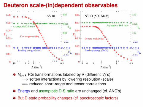
Deuteron scale-(in)dependent observables
0.51234510
Λ (fm−1
)
0
0.01
0.02
0.03
0.04
0.05
0.06
PD
−2.23
−2.225
−2.22
ED
0.02
0.025
0.03
ηsd
AV18
D-state probability
Asymptotic D-S ratio
Binding energy (MeV)
0.512345
Λ (fm−1
)
0
0.01
0.02
0.03
0.04
0.05
0.06
PD
−2.23
−2.225
−2.22
ED
0.02
0.025
0.03
ηsd
N3LO (500 MeV)
D-state probability
Asymptotic D-S ratio
Binding energy (MeV)
Vlow k RG transformations labeled by Λ (different VΛ’s)=⇒ soften interactions by lowering resolution (scale)=⇒ reduced short-range and tensor correlations
Energy and asymptotic D-S ratio are unchanged (cf. ANC’s)
But D-state probability changes (cf. spectroscopic factors)

Unevolved long-distance operators change slowly with λ
Matrix elements dominated by longrange run slowly for λ > 2 fm−1
Here: examples from the deuteron(compressed scales)
Which is the correct answer?
Are we using the completeoperator for the experimentalquadrupole moment?
1 1.5 2 2.5 3 3.5 4λ [fm−1]
1.95
2.00
2.05
2.10
bare
r d [fm
] N3LO (550/600 MeV)Vsrg
Deuteron rms radius
1 1.5 2 2.5 3 3.5 4
λ [fm−1]
0.2
0.22
0.24
0.26
0.28
0.3
bare
Qd [f
m2 ]
N3LO (550/600 MeV)Vsrg
Deuteron quadrupole expt.
1 1.5 2 2.5 3 3.5 4λ [fm−1]
0.36
0.38
0.40
0.42
0.44
0.46
bare
<1/
r>
N3LO (550/600 MeV)Vsrg
Deuteron <1/r>
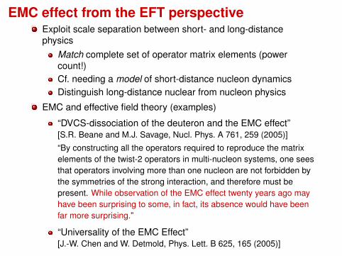
EMC effect from the EFT perspectiveExploit scale separation between short- and long-distancephysics
Match complete set of operator matrix elements (powercount!)Cf. needing a model of short-distance nucleon dynamicsDistinguish long-distance nuclear from nucleon physics
EMC and effective field theory (examples)
“DVCS-dissociation of the deuteron and the EMC effect”[S.R. Beane and M.J. Savage, Nucl. Phys. A 761, 259 (2005)]
“By constructing all the operators required to reproduce the matrixelements of the twist-2 operators in multi-nucleon systems, one seesthat operators involving more than one nucleon are not forbidden bythe symmetries of the strong interaction, and therefore must bepresent. While observation of the EMC effect twenty years ago mayhave been surprising to some, in fact, its absence would have beenfar more surprising.”
“Universality of the EMC Effect”[J.-W. Chen and W. Detmold, Phys. Lett. B 625, 165 (2005)]

Dependence of EMC effect on A is long-distance physics!EFT treatment by Chen and Detmold [Phys. Lett. B 625, 165 (2005)]
F A2 (x) =
∑i
Q2i xqA
i (x) =⇒ RA(x) = F A2 (x)/AF N
2 (x)
“The x dependence of RA(x) is governed by short-distancephysics, while the overall magnitude (the A dependence) ofthe EMC effect is governed by long distance matrix elementscalculable using traditional nuclear physics.”
Match matrix elements: leading-order nucleon operators toisoscalar twist-two quark operators =⇒ parton dist. moments
J.-W. Chen, W. Detmold / Physics Letters B 625 (2005) 165–170 167
symmetries [14–17]. The leading one- and two-bodyhadronic operators in the matching are
(4)Oµ0···µn
q =!xn
"qvµ0 · · ·vµnN†N
#1+ !nN
†N$+ · · · ,
where vµ = vµ + O(1/M) is the velocity of thenucleus. Operators involving additional derivativesare suppressed by powers of M in the EFT power-counting. In Eq. (4) we have only kept the SU(4) (spinand isospin) singlet two-body operator !nv
µ0 · · ·!vµn(N†N)2. The other independent two-body oper-ator "nv
µ0 · · ·vµn(N†!N)2, which is non-singlet inSU(4) (! is an isospin matrix), is neglected because"n/!n = O(1/N2
c ) " 0.1 [21], where Nc is the num-ber of colors. Furthermore, the matrix element of(N†!N)2 for an isoscalar state with atomic num-ber A is smaller than that of (N†N)2 by a factor A
[10]. Three- and higher-body operators also appear inEq. (4); numerical evidence from other EFT calcula-tions indicates that these contributions are generallymuch smaller than two-body ones [22].Nuclear matrix elements of Oµ0···µn
q give the mo-ments of the isoscalar nuclear parton distributions,qA(x). The leading order (LO) and the next-to-leadingorder (NLO) contributions to these matrix elementsare shown in Fig. 1(a) and (b), respectively. For an un-polarised, isoscalar nucleus,
!xn
"q|A # vµ0 · · ·vµn$A|Oµ0···µn
q |A%
(5)=!xn
"q
#A + $A|!n
%N†N
&2|A%$,
where we have used $A|N†N |A% = A. Notice that ifthere were no EMC effect, the !n would vanish forall n. Also !0 = 0 because of charge conservation. As-ymptotic relations [23] and analysis of experimentaldata [2,24] suggests that !1 " 0, implying that quarkscarry very similar fractions of a nucleon’ and a nucle-us’ momentum though no symmetry guarantees this.From Eq. (5) we see that the ratio
(6)$xn%q|AA$xn%q & 1$xm%q|AA$xm%q & 1
= !n
!m
is independent ofAwhich has powerful consequences.In all generality, the isoscalar nuclear quark distribu-tion can be written as
(7)qA(x) = A#q(x) + g(x,A)
$.
Taking moments of Eq. (7), Eq. (6) then demands thatthe x dependence and A dependence of g factorise,
(8)g(x,A) = g(x)G(A),
with
(9)G(A) = $A|%N†N
&2|A%/A#30,
and g(x) satisfying
(10)!n = 1#30$xn%q
A'
&A
dx xng(x).
#0 is an arbitrary dimensionful parameter and will bechosen as #0 = 1 fm&1. Crossing symmetry dictates
Fig. 1. Contributions to nuclear matrix elements. The dark square represents the various operators in Eq. (4) and the light shaded ellipsecorresponds to the nucleus, A. The dots in the lower part of the diagram indicate the spectator nucleons.
=⇒ 〈xn〉qvµ0 · · · vµn N†N[1 + αnN†N] + · · ·
RA(x) =F A
2 (x)
AF N2 (x)
= 1+gF2 (x)G(A) where G(A) = 〈A|(N†N)2|A〉/AΛ0
=⇒ the slope dRAdx scales with G(A) [Why is this not cited more?]
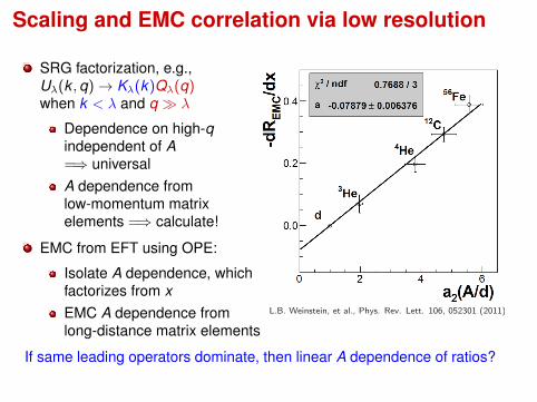
Scaling and EMC correlation via low resolution
SRG factorization, e.g.,Uλ(k ,q)→ Kλ(k)Qλ(q)when k < λ and q � λ
Dependence on high-qindependent of A=⇒ universalA dependence fromlow-momentum matrixelements =⇒ calculate!
EMC from EFT using OPE:
Isolate A dependence, whichfactorizes from xEMC A dependence fromlong-distance matrix elements
Short Range Correlations and the EMC e!ect
Deep inelastic scattering ratio atQ2 ! 2GeV2 and 0.35 " xB " 0.7and inelastic scattering atQ2 ! 1.4GeV2 and 1.5 " xB " 2.0
Strong linear correlation betweenslope of ratio of DIS cross sections(nucleus A vs. deuterium) andnuclear scaling ratio
SRG Factorization at leading order:# Dependence on high-q
is independent of A# A-dependence from low
momentum matrix elementindependent of operator
L.B. Weinstein, et al., Phys. Rev. Lett. 106, 052301 (2011)
Why should A-dependence of nuclear scaling a2 and the EMC e!ect bethe same?
Overview Operators Factorization Conclusions Principles Applications
If same leading operators dominate, then linear A dependence of ratios?

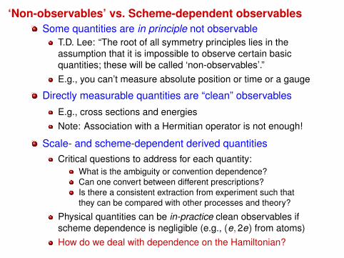
‘Non-observables’ vs. Scheme-dependent observablesSome quantities are in principle not observable
T.D. Lee: “The root of all symmetry principles lies in theassumption that it is impossible to observe certain basicquantities; these will be called ‘non-observables’.”E.g., you can’t measure absolute position or time or a gauge
Directly measurable quantities are “clean” observables
E.g., cross sections and energiesNote: Association with a Hermitian operator is not enough!
Scale- and scheme-dependent derived quantitiesCritical questions to address for each quantity:
What is the ambiguity or convention dependence?Can one convert between different prescriptions?Is there a consistent extraction from experiment such thatthey can be compared with other processes and theory?
Physical quantities can be in-practice clean observables ifscheme dependence is negligible (e.g., (e,2e) from atoms)How do we deal with dependence on the Hamiltonian?

Scale/scheme dependence: spectroscopic factors
Green’s functions I 19
RemovalRemovalprobability forprobability forvalence protonsvalence protons
fromfromNIKHEF dataNIKHEF data
Note:We have seen mostlydata for removal of
valence protons
Spectroscopic factors for valenceprotons have been extracted from(e,e′p) experimental crosssections (e.g., Nikhef 1990’s at left)
Used as canonical evidence for“correlations”, particularlyshort-range correlations (SRC’s)
But if SFs are scale/schemedependent, how do we explainthe cross section?
12C(e, e!p)X
1966 1988 2006

(Assumed) factorization of (e,e′p) cross section
958 M. LEUSCHNER et al. 49
TABLE II. Kinematics of the ' O(e, e'p) "N experiment. T, is the total center-of-mass kinetic en-ergy between the recoi1ing "N nucleus and the knocked out proton, aud Q is the total charge accumu-lated at each kinematics.
Pm(MeV/e)—150.5—100.1—81.5—40.8
1.839.479.4118.9159.4191.6216.5250.5
Eo(MeV)
520.6520.6455.8455.8520.6455.8455.8455.8455.8455.8304.4304.4
0,(deg)
78.378.081.272.858.557.149.742.535.329.340.630.2
Pe'(MeV/c)
405.63&8.8335.4336.9397.0339.7340.8341.7342.5342.4188.9196.1
Op
(deg)
42.240.839.542.247.446.548.048.748.547.138.236.0
Pp(MeV/c)
441.1481.6441.7438.9460.2433.0430.0427. 1424. 1421.7419.1417.6
Tc.m.(MeV)
87.7105.589.990.099.790.090.090.090.090.089.690.0
(mC)
250.0310.065.7209.765.1150.0118.2110.061.043.2130.036.5
tions which reflected the complete (E,p ) dependenceof the accidental coincidence spectrum on the spectrome-ter geometry. For the present analysis, adjustments inthe position of the electron spectrometer aperture of upto 5 rnrad in the horizontal direction and 4 mrad in thevertical direction were required. Adjustments of thesemagnitudes are within the alignment tolerances of thespectrometer, beam, and target system. For the protonspectrometer, the data were found to be insensitive tosmall changes in the aperture osition.The coincidence reaction ' O(e, e'p)' N was measured
in quasielastic parallel kinematics at three different beamenergies: ED=304, 456, and 521 MeV. The total kineticenergy in the center-of-mass system between the outgoingproton and the recoiling ' N nucleus was kept constant at90 MeV. Table II lists the relevant kinematical pararne-ters of the experiment.For the present experiment, we have measured the ' 0
spectral function in the range 0&E &40 MeV and—180& p & 270 MeV jc. The sign of the missingmomentum refers to the projection of the initial nucleonmomentum along the direction of the momentumtransfer. The missing rnomenturn is positive for~q~ & ~p'~. In Fig. 1 a missing energy spectrum of the re-action ' O(e, e'p)' N is shown for the kinematics cen-tered about p =120 MeV/c. The spectrum is dominat-ed by two peaks at E =12.1 and 18.4 MeV, correspond-ing to proton knockout from the valence 1p orbitals in' O. The missing energy resolution obtained for the ex-periment varied between 150 and 200 keV for thedifFerent kinematics. Because of this excellent resolution,the excitation of the ' N positive parity doublet atE„=5.3 MeV (E =17.4 MeV) is also clearly evident.The momentum distribution can be calculated for eachdiscrete state in the spectral function by integrating overthe missing energy interval of interest [see expression (4)].
IV. DWIA ANALYSIS
Distortions of the knocked out proton wave functionrequired for the DWIA analysis were calculated using
2OO 1
16p{e e p)1SN
80 & p ( 160 MeV/c l
3/8
15O—&D
100E
5o I-
t
5/2'1/2+
14 16 18 20E [Mev]
3/2
22 24 26
FIG. 1. ' O(e, e'p) "N missing energy spectrum for the kine-matics centered about p = 120MeV/e.
6ve different optical potentials. Three of the optical po-tentials were phenomenological Woods-Saxon parametri-zations. Of these, two were derived directly from elastic' O(p,p') data [17] taken at an incident laboratory energyof 100 MeV. The elastic cross section and analyzingpower were fit [18] with a Woods-Saxon (WS) potentialcontaining real, imaginary, and spin-orbit terms. Asecond potential (WSdd), which included two additionalderivative terms in the central potential, was also used toflt the (p,p') data. The center-of-mass kinetic energy of90 MeV for the current (e, e'p) experiment corresponds
Missing energy spectrum for16O(e, e′p)15N [Leuschner (1994)]
M. LEUSCHNER et al.
The final fitted DWIA results for the two strong 1ptransitions are shown in Fig. 3. The extracted spectro-scopic factors and rms radii for each state and each po-tential are listed in Table IV. All five potentials yield ex-cellent fits for both states. The quality of the fit, as evi-denced by the g values listed in Table IV, does not sufferwith the inclusion of the data at p &0. Furthermore,the extracted values of r, and S do not depend onwhether or not the p &0 data are included in the fit.The spectroscopic factors obtained from the current
experiment are in general agreement with those of theprevious ' O(e, e'p) experiment of Bernheim et al. [4], al-though their analysis employed different bound statewave functions and different optical potentials, and theirdata were taken in a difFerent kinematical arrangement(nonparallel). They reported spectroscopic factors of1.18(15) and 2.28(29) for the lp&zz ground state and i@3&2third excited state, respectively.As Table VI indicates, the consistency among the fitted
parameters between the five potentials is excellent for theground state transition, while the spectroscopic fac-
tors for the —,' state at E„=6.3 MeV differ by almost
20% between the extreme values. The spectroscopic fac-tors from the WS and WSdz potentials, which were bothderived from elastic (p,p') data, agree to within a fewpercent. The results from the two Kelly potentials,which were derived explicitly from inelastic (p,p') data,are also close to one another. The magnitude of the spec-troscopic factor due to the Schwandt parametrizationfalls between the first two groups. The major discrepancyconcerns results which were derived using optical poten-tials which describe elastic (p,p') data and optical poten-tials which describe inelastic (p,p') data. Since all fivepotentials give a good (y /ND„&1) description of theelastic (p,p') data and the (e, e'p) momentum distribu-tions, we conclude that the optical potential is notsuSciently constrained by the elastic (p,p') scatteringdata alone.The weak transitions to the positive parity states atE„=5.3 MeV in ' N are of particular interest for deter-mining the structure of ' O. The momentum distribution
100WsddKe190nSC
P3/aE„= 6.3 MeV
0. 1
PiE„
—200 —100I
0 100P [Mev,/c]
200
FIG. 3. Momentum distribution for 1p&/2 ground state (bot-tom) and the 1p3/2 state at E„=6.3 MeV. The curves representDWIA calculations using three difFerent optical potentials.
for this doublet is shown in Fig. 4. The DWIA analysisof these states is complicated somewhat because they arenot resolved in missing energy, since the 30 keV separa-tion energy between the two states is considerably lessthan the experimental resolution of 150—200 keV. Be-cause the two states differ in their angular momentum, aseparation in missing momentum can be performed.In order to extract the rms radii and spectroscopic fac-
tors, the measured momentum distribution was fit withan incoherent sum of 2s&&2 and 1d5/2 momentum distri-butions. The radii and spectroscopic factors of each statewere allowed to vary independently. The extracted spec-
TABLE IV. Spectroscopic results for ' 0 proton knockout leading to the lp&/2 "N ground state andthe 1p3/2 state at E„=6.3 MeV. The errors represent the statistical uncertainties only. The overall sys-tematic uncertainty for the present data is 5.4%.
State(J77)
E„(MeV) Potential
Radius(fm)
p )0S X'~&DF
Radius(fm)
All p
S X'~&DFl—2 0.00 WS
WSddSc
Ke196nKe1100o
2.918(32)2.928( 33 )2.828( 31)2.958(31)2.991(31)
1.261( 13)1.230( 16)1.222( 11)1.249( 18)1.221( 13)
0.640.700.600.630.67
2.898(31)2.906(36)2.835(30)2.943(30)2.970(29)
1.275( 18)1.242( 17)1.220( 11)1.260( 13)1.234( 16)
0.720.770.570.670.85
32 6.32 WS
WSddSc
Ke196nKe1100o
2.775(21 )2.778(47)2.677(21 )2.727(25 )2.793(23)
2.047( 14)1.980(15)2.132( 14)2.339(18)2.232(15)
1.161.270.660.700.77
2.771(20)2.784(22)2.680( 19)2.719(24)2.805( 15)
2.059( 16)1.983(16)2.132( 12)2.348( 19)2.215( 12)
0.981.070.690.720.92
dσdp′edp′N
= Kσep × ρ(pm) ∝ |φα(pm)|2
=⇒ p1/2 spectroscopic factor ≈ 0.63

(Assumed) factorization of (e,e′p) cross section!"!#$%
!"&#$%
!'!#$%
!"!#$%
!"&#$%
!'!#$%
!()*'%
!+,*'%
!"!#$-"./"
Knock out p1/2 proton from 16O to15N ground state in IPM
Adjust s.p. well depth and radius toidentify φα(pm)
Final state interactions (FSI) addedusing optical potential(s)
M. LEUSCHNER et al.
The final fitted DWIA results for the two strong 1ptransitions are shown in Fig. 3. The extracted spectro-scopic factors and rms radii for each state and each po-tential are listed in Table IV. All five potentials yield ex-cellent fits for both states. The quality of the fit, as evi-denced by the g values listed in Table IV, does not sufferwith the inclusion of the data at p &0. Furthermore,the extracted values of r, and S do not depend onwhether or not the p &0 data are included in the fit.The spectroscopic factors obtained from the current
experiment are in general agreement with those of theprevious ' O(e, e'p) experiment of Bernheim et al. [4], al-though their analysis employed different bound statewave functions and different optical potentials, and theirdata were taken in a difFerent kinematical arrangement(nonparallel). They reported spectroscopic factors of1.18(15) and 2.28(29) for the lp&zz ground state and i@3&2third excited state, respectively.As Table VI indicates, the consistency among the fitted
parameters between the five potentials is excellent for theground state transition, while the spectroscopic fac-
tors for the —,' state at E„=6.3 MeV differ by almost
20% between the extreme values. The spectroscopic fac-tors from the WS and WSdz potentials, which were bothderived from elastic (p,p') data, agree to within a fewpercent. The results from the two Kelly potentials,which were derived explicitly from inelastic (p,p') data,are also close to one another. The magnitude of the spec-troscopic factor due to the Schwandt parametrizationfalls between the first two groups. The major discrepancyconcerns results which were derived using optical poten-tials which describe elastic (p,p') data and optical poten-tials which describe inelastic (p,p') data. Since all fivepotentials give a good (y /ND„&1) description of theelastic (p,p') data and the (e, e'p) momentum distribu-tions, we conclude that the optical potential is notsuSciently constrained by the elastic (p,p') scatteringdata alone.The weak transitions to the positive parity states atE„=5.3 MeV in ' N are of particular interest for deter-mining the structure of ' O. The momentum distribution
100WsddKe190nSC
P3/aE„= 6.3 MeV
0. 1
PiE„
—200 —100I
0 100P [Mev,/c]
200
FIG. 3. Momentum distribution for 1p&/2 ground state (bot-tom) and the 1p3/2 state at E„=6.3 MeV. The curves representDWIA calculations using three difFerent optical potentials.
for this doublet is shown in Fig. 4. The DWIA analysisof these states is complicated somewhat because they arenot resolved in missing energy, since the 30 keV separa-tion energy between the two states is considerably lessthan the experimental resolution of 150—200 keV. Be-cause the two states differ in their angular momentum, aseparation in missing momentum can be performed.In order to extract the rms radii and spectroscopic fac-
tors, the measured momentum distribution was fit withan incoherent sum of 2s&&2 and 1d5/2 momentum distri-butions. The radii and spectroscopic factors of each statewere allowed to vary independently. The extracted spec-
TABLE IV. Spectroscopic results for ' 0 proton knockout leading to the lp&/2 "N ground state andthe 1p3/2 state at E„=6.3 MeV. The errors represent the statistical uncertainties only. The overall sys-tematic uncertainty for the present data is 5.4%.
State(J77)
E„(MeV) Potential
Radius(fm)
p )0S X'~&DF
Radius(fm)
All p
S X'~&DFl—2 0.00 WS
WSddSc
Ke196nKe1100o
2.918(32)2.928( 33 )2.828( 31)2.958(31)2.991(31)
1.261( 13)1.230( 16)1.222( 11)1.249( 18)1.221( 13)
0.640.700.600.630.67
2.898(31)2.906(36)2.835(30)2.943(30)2.970(29)
1.275( 18)1.242( 17)1.220( 11)1.260( 13)1.234( 16)
0.720.770.570.670.85
32 6.32 WS
WSddSc
Ke196nKe1100o
2.775(21 )2.778(47)2.677(21 )2.727(25 )2.793(23)
2.047( 14)1.980(15)2.132( 14)2.339(18)2.232(15)
1.161.270.660.700.77
2.771(20)2.784(22)2.680( 19)2.719(24)2.805( 15)
2.059( 16)1.983(16)2.132( 12)2.348( 19)2.215( 12)
0.981.070.690.720.92
dσdp′edp′N
= Kσep × ρ(pm) ∝ |φα(pm)|2
=⇒ p1/2 spectroscopic factor ≈ 0.63

Deuteron electromagnetic form factors
GC , GQ , GM in deuteron withchiral EFT at leading order(Valderrama et al.)
NNLO 550/600 MeV potential
Unchanged at low q withunevolved operators
Independent of λ with evolvedoperators
0 1 2 3 4 510
−3
10−2
10−1
100
q (fm−1
)
GC
λ=1.5
Unevolved
SRG EvolvedSRG Evolved wfwith Bare Operator
0 1 2 3 4 510
−3
10−2
10−1
100
q (fm−1
)
GQ
λ=1.5
Unevolved
SRG EvolvedSRG Evolved wfwith Bare Operator
0 1 2 3 4 510
−3
10−2
10−1
100
q (fm−1
)
MG
M/M
d
λ=1.5
Unevolved
SRG Evolved
SRG Evolved wfwith Bare Operator

Generic knockout reaction [e.g., Dickhoff/Van Neck text]Consider a scalar external probe that just transfers momentum q
ρ(q) = ρ0
A∑j=1
e−iq·r =⇒ ρ(q) = ρ0
∑p,p′
〈p|e−iq·r|p′〉a†pap′q
p!
p
First assumption: one-body operator (scale dependent!)
Then the cross section from Fermi’s golden rule is
dσ ∼∑
δ(ω + Ei − Ef )|〈Ψf |ρ(q)|Ψi〉|2
Complication: ejected final particle A interacts on way out (FSI)
HA =A∑
i=1
p2i
2m+
A∑i<j=1
V (i , j) = HA−1 +p2
A2m
+A−1∑i=1
V (i ,A)
If we neglect this interaction =⇒ PW (no FSI)
|Ψi〉 = |ΨA0 〉 , |Ψf 〉 = a†p|ΨA−1
n 〉 =⇒ 〈Ψf | = 〈ΨA−1n |ap
=⇒ factorized knockout cross section ∝ hole spectral fcn:
dσ ∼ ρ20
∑n
δ(Em − EA0 + EA−1
n )|〈ΨA−1n |apm |ΨA
0 〉|2 = ρ20 Sh(pm,Em)
Does it still factorize when corrected for (scale dependent!) FSI?

Now repeat with a unitary transformation U
The cross section is guaranteed to be the same from U†U = 1
dσ ∼∑
δ(ω + Ei − Ef )|〈Ψf |ρ(q)|Ψi〉|2
=∑
δ(ω + Ei − Ef )|〈Ψf |(U†U)ρ(q)(U†U)|Ψi〉|2
=∑
δ(ω + Ei − Ef )|(〈Ψf |U†)(Uρ(q)U†)(U|Ψi〉)|2
but the pieces are different now.
Schematically, the SRG has U = 1 + 12 (U − 1)a†a†aa + · · ·
U is found by solving for the unitary transformation in theA = 2 system (this is the easy part!)The · · · ’s represent higher-body operatorsOne-body operators (∝ a†a) gain many-body pieces(EFT: there are always many-body pieces at some level!)Both initial and final states are modified (and therefore FSI)

New pieces after the unitary transformation
The current is no longer just one-body (cf. EFT current):
Uρ(q)U† = + α + · · ·
New correlations have appeared (or disappeared):
U|ΨA0 〉 = U
12C(e, e!p)X
1966 1988 2006
+ · · · =⇒
12C(e, e!p)X
1966 1988 2006
+ α
12C(e, e!p)X
1966 1988 2006
+ · · ·
Similarly with |Ψf 〉 = a†p|ΨA−1n 〉
So the spectroscopic factors are modified
Final state interactions are also modified by U
Bottom line: the cross section is unchanged only if all pieces areincluded, with the same U: H(λ), current operator, FSI, . . .

Changing resolution shifts physics: Not unique!
From D. Higinbotham, arXiv:1010.4433
A−1A
q
A
q
e e
e’ e’
a) b)
A−2
N
NN
“The simple goal of short-range nucleon-nucleon correlation studiesis to cleanly isolate diagram b) from a). Unfortunately, there aremany other diagrams, including those with final-state interactions,that can produce the same final state as the diagram scientists wouldlike to isolate. If one could find kinematics that were dominated bydiagram b) it would finally allow electron scattering to provide newinsights into the short-range part of the nucleon-nucleon potential.”
What is in the blob in b)? A one-body vertex and an SRC, or atwo-body vertex? Depends on the resolution! (Also FSI+ will mix.)

Deuteron-like scaling at high momenta from factorization
Deuteron vs Complex Nuclei at high momentum region
C. Ciofi and S. Simula, Phys.Rev C53, 1689(1996)
n(k) at high Momentum regions are similar to it of the Deuteron
Momentum Distributions n(k) Ratio to the Deuteron
2H
3He,4He,16O, 56Fe and N.M.
Almost Flat! High resolution: Dominance of VNN and SRCs (Frankfurt et al.)
Lower resolution =⇒ lower separation scale =⇒ fall-off depends onVλ