Applications of Machine Learning and ComputationalLinguistics in Financial Economics

Lili Gao

April 2016

CARNEGIE MELLON UNIVERSITY

Applications of Machine Learning and Computational Linguistics in

Financial Economics

A dissertation

submitted to the Tepper School of Business

in partial fulfillment of the requirements for the degree of

Doctor of Philosophy

Field of Economics

by

Lili Gao

April 2016

Dissertation Committee

Bryan Routledge (Chair)

Stefano Sacchetto

Steve Karolyi

Alan Montgomery (Outside Reader)

c©2016

Lili Gao

All Rights Reserved

Abstract

In the world of the financial economics, we have abundant text data. Articles in the Wall

Street Journal and on Bloomberg Terminals, corporate SEC filings, earnings-call

transcripts, social media messages, etc. all contain ample information about financial

markets and investors’ behaviors. Extracting meaningful signals from unstructured and

high dimensional text data is not an easy task. However, with the development of machine

learning and computational linguistic techniques, processing and statistically analyzing

textual documents tasks can be accomplished, and many applications of statistical text

analysis in social sciences have proven to be successful.

In my thesis, I conduct statistical text analysis using datasets constructed from the

SEC corporate filings to retrieve information about the financial market macroeconomic

conditions. First, using the text data from the management discussions and analysis in

corporate annual reports (10-K files), I examine whether the management discussions contain

information that reveals a firm’s exposure to systematic risk, and construct a risk factor

based on textual information that can explain the cross-sectional variations in expected

stock returns (Chapter 1). Second, using a text dataset containing letters to shareholders

written by institutional investment managers, I analyze whether fund manager discussions

provide insights in predicting returns of the aggregate market portfolio (Chapter 2). In

addition to conducting empirical tests in asset pricing using textual data. I also construct a

theoretical model to explain the interaction between corporate takeover activities and cash

holdings behaviors, and I calibrate my model to the U.S. market mergers and acquisitions

i

data (Chapter 3).

I demonstrate a variety of machine learning, natural language processing and dynamic

programming techniques as powerful tools in complement to traditional econometric

methods commonly adopted by economists. My work illustrates the potential of using text

data as a new avenue for empirical research in financial economics. In particular, although

computational linguistic techniques have made significant achievements in social sciences

such as political science and sociology, and they have also drawn lots of attention from

financial industry practitioners, their applications in financial economics academic research

is still limited. My work aims to fill this gap.

ii

Acknowledgments

I would like to thank my advisor, Professor Bryan Routledge, for his tremendous help,

enlightenment, and support. Bryan sets up an example for me to be rigorous in research,

and to be passionate in solving interesting and challenging problems. Every time I talk

with Bryan, I learn something new, feel stuffed with brilliant insights and inspired with full-

hearted motivation. Our conversations strengthened my conviction to be a researcher and

contribute knowledge to the fascinating field of the intersection between machine learning,

computational linguistics, and financial economics.

I am sincerely obliged to Professor Stefano Sacchetto. It was Stefano who guided me to

start doing research in the captivating field of financial economics since my first year as a

Ph.D. student at Tepper. Stefano urged me to read plenty of classical papers in corporate

finance, directed me to develop research ideas, carefully proofread my paper drafts, and

provided lots of invaluable advice in preparing myself to be a qualified researcher.

I am deeply grateful to Professor Steve Karolyi, who gave me lots of crucial guidance in

conducting empirical research. Steve always asks discerning questions, which helped me to

discover the missing or weak point in my research and stimulated many research ideas. He

also gave me thorough and insightful suggestions on my career development.

I feel incredibly fortunate to have worked closely with Professor Alan Montgomery. As

the outside reader for my economics Ph.D. dissertation, Alan encouraged me to think about

financial economics from different angles, which greatly benefited me in crafting innovative

research ideas. As my mentor in the machine learning master program, Alan gave me great

iii

advice in applying my computer science skills in the financial economics research.

I benefited enormously from a number of faculty members of CMU: Professor Laurence

Ales, Professor Andrew Bird, Professor Carlos Corona, Professor Anisha Ghosh, Professor

Brent Glover, Professor Geoff Gordon, Professor Isa Hafalir, Professor Burton Hollifield,

Professor Yaroslav Kryukov, Professor Lars-Alexander Kuehn, Professor Jing Li, Professor

Pierre Jinghong Liang, Professor Bennett Mccallum, Professor Robert Miller, Professor

Emilio Osambela, Professor R. Ravi, Professor Thomas Ruchti, Professor Alan

Scheller-Wolf, Professor Steven Shreve, Professor Christopher Sleet, Professor Fallaw

Sowell, Professor Chester Spatt, Professor Steve Spear, Professor Ryan Tibshirani,

Professor Larry Wasserman, Professor Shu Lin Wee, Professor Eric Xing, Professor Yiming

Yang, Professor Sevin Yeltekin, Professor Ariel Zetlin-Jones, and many others.

Thanks to Lawrence Rapp for the continuous and superior help.

I am appreciative to have many friends who made my Ph.D. studies a fruitful and

enjoyable journey of my life. Special thanks go to Aaron Barkley, Francisco Cisternas, Alex

Kazachkov, Qihang Lin, Xiao Liu, Eric Siyu Lu, Yifei Ma, Ronghuo Zheng and others.

Finally, I want to give my deepest thanks to my fiancee who granted me so much help

and support in both my work and life, and my parents who directed me to pursue knowledge

and truth since I was a child. This dissertation is dedicated to my fiancee Tianjiao Dai, my

mother Yaqiong Zhou and my father Shan Gao.

iv

Contents

1 Text-implied Risk and the Cross-section of Expected Stock Returns 4

1.1 Introduction . . . . . . . . . . . . . . . . . . . . . . . . . . . . . . . . . . . . 5

1.2 Beta Pricing Model . . . . . . . . . . . . . . . . . . . . . . . . . . . . . . . . 10

1.3 Text-based Risk Measure . . . . . . . . . . . . . . . . . . . . . . . . . . . . . 11

1.4 Empirical Results . . . . . . . . . . . . . . . . . . . . . . . . . . . . . . . . . 18

1.4.1 Data Description . . . . . . . . . . . . . . . . . . . . . . . . . . . . . 18

1.4.2 Estimate γ . . . . . . . . . . . . . . . . . . . . . . . . . . . . . . . . . 21

1.4.3 Estimate Document Risk Score DRS . . . . . . . . . . . . . . . . . . 24

1.4.4 Beta Sorted Portfolios . . . . . . . . . . . . . . . . . . . . . . . . . . 25

1.4.5 Robustness . . . . . . . . . . . . . . . . . . . . . . . . . . . . . . . . 27

1.4.6 Price of the Text-implied Risk . . . . . . . . . . . . . . . . . . . . . . 30

1.5 Economic Intuition of the Text-implied Factor . . . . . . . . . . . . . . . . . 31

1.5.1 TXT and Macroeconomic Variables . . . . . . . . . . . . . . . . . . . 31

1.6 Conclusion . . . . . . . . . . . . . . . . . . . . . . . . . . . . . . . . . . . . . 34

1.A Appendix . . . . . . . . . . . . . . . . . . . . . . . . . . . . . . . . . . . . . 35

2 Investment Manager Discussions and Stock Returns 60

2.1 Introduction . . . . . . . . . . . . . . . . . . . . . . . . . . . . . . . . . . . . 61

2.2 Language Model . . . . . . . . . . . . . . . . . . . . . . . . . . . . . . . . . . 65

2.2.1 CBOW . . . . . . . . . . . . . . . . . . . . . . . . . . . . . . . . . . . 66

i

2.2.2 Matrix Factorization . . . . . . . . . . . . . . . . . . . . . . . . . . . 69

2.3 Data . . . . . . . . . . . . . . . . . . . . . . . . . . . . . . . . . . . . . . . . 70

2.3.1 Letters to Shareholders . . . . . . . . . . . . . . . . . . . . . . . . . . 70

2.3.2 Stock Returns . . . . . . . . . . . . . . . . . . . . . . . . . . . . . . . 73

2.4 Empirical Results . . . . . . . . . . . . . . . . . . . . . . . . . . . . . . . . . 74

2.4.1 Word Vectors . . . . . . . . . . . . . . . . . . . . . . . . . . . . . . . 74

2.4.2 Word Clouds . . . . . . . . . . . . . . . . . . . . . . . . . . . . . . . 74

2.4.3 Out-of-sample Predictions . . . . . . . . . . . . . . . . . . . . . . . . 76

2.4.4 Comparison with Other Language Models . . . . . . . . . . . . . . . 80

2.4.5 Stock Return Volatilities . . . . . . . . . . . . . . . . . . . . . . . . . 83

2.4.6 Macro Economic Variables . . . . . . . . . . . . . . . . . . . . . . . . 84

2.5 Economic Interpretation . . . . . . . . . . . . . . . . . . . . . . . . . . . . . 86

2.6 Conclusion . . . . . . . . . . . . . . . . . . . . . . . . . . . . . . . . . . . . . 88

2.A Appendix . . . . . . . . . . . . . . . . . . . . . . . . . . . . . . . . . . . . . 90

3 Corporate Takeovers and Cash Holdings 99

3.1 Introduction . . . . . . . . . . . . . . . . . . . . . . . . . . . . . . . . . . . . 100

3.2 Model . . . . . . . . . . . . . . . . . . . . . . . . . . . . . . . . . . . . . . . 103

3.3 Calibration . . . . . . . . . . . . . . . . . . . . . . . . . . . . . . . . . . . . 110

3.3.1 Data . . . . . . . . . . . . . . . . . . . . . . . . . . . . . . . . . . . . 110

3.3.2 Parametrization and calibration targets . . . . . . . . . . . . . . . . . 110

3.4 Numerical results and comparative statics . . . . . . . . . . . . . . . . . . . 112

3.4.1 Cash comparative statics . . . . . . . . . . . . . . . . . . . . . . . . . 113

3.4.2 Acquisition activity comparative statics . . . . . . . . . . . . . . . . . 114

3.4.3 Entry and exit . . . . . . . . . . . . . . . . . . . . . . . . . . . . . . 115

3.4.4 Acquirer and Target Value Difference . . . . . . . . . . . . . . . . . . 117

3.4.5 Summary . . . . . . . . . . . . . . . . . . . . . . . . . . . . . . . . . 118

3.5 Conclusion . . . . . . . . . . . . . . . . . . . . . . . . . . . . . . . . . . . . . 118

ii

3.A Appendix . . . . . . . . . . . . . . . . . . . . . . . . . . . . . . . . . . . . . 120

3.A.1 Numerical solution . . . . . . . . . . . . . . . . . . . . . . . . . . . . 120

3.A.2 Simulation Algorithm . . . . . . . . . . . . . . . . . . . . . . . . . . . 121

iii

Introduction

Well structured numerical data have long been the main source for empirical studies in

financial economics. Although financial text data like journal articles, corporate regulatory

filings, earnings call scripts, social media messages are more abundant than numerical ones,

regarding both amount and public availability, they have been utilized in a quite limited

number of financial economics academic research. One of the main reasons is that text

data are usually unstructured, fragmented and in very high dimension in nature, making

the traditional data analysis tools familiar to financial economics researchers like

regressions powerless. With the development of natural language processing and machine

learning techniques in computational linguistics, analyzing text information in a

systematical and efficient way is easier than ever and has attracted considerable attention

from researchers in different disciplines, which also opens up a new avenue for empirical

research in financial economics.

My research is dedicated to investigating and developing methodologies to efficiently

extract financial market and corporate information contained in public available corporate

SEC filings text data, and to understand its implications on the financial market and investor

behaviors. In addition to testing economic theories by conducting empirical research, I

build a theoretical model to investigate the covariation between corporate takeover activities

and cash holding behaviors and calibrate the model to the SDC U.S. market mergers and

acquisitions dataset.

In the first chapter, I analyze the informativeness of text data contained in the

1

management discussion and analysis section of SEC 10-K files about stock returns. I used

the popular bag-of-words model in the computational linguistic literature to represent

documents. In particular, each document can be represented as a vector of words. Each

entry of the vector corresponds to a unique word in the vocabulary, and the value of each

entry is the weight (can be counts, frequency, tf-idfs etc.) assigned to the word. The

underlying assumption of the bag-of-words models is that the token position information is

irrelevant. Although this assumption seems strong, the bag-of-words model usually

generates robust results when trained using large corpus. To summarize the stock return

information contained in the high dimensional text data into a one-dimensional text factor,

I used multinomial inverse regression to project document word vectors onto a

one-dimensional subspace that is most relevant to the stock returns, generating the

document risk score (DRS), which measures the exposure to the underlying systematic

risk for each individual stock. I construct a factor mimicking portfolio TXT for the

text-implied risk by sorting stocks based on DRS and estimate its risk premium, which is

found to be significant and positive. I also investigated the economic meaning of the

text-implied systematic risk and find the it is related the real productivity shocks and

financial market volatilities.

In the second chapter, I investigate whether institutional investment managers have

market insights. To answer my question, I test whether letters to shareholders written by

investment managers contain useful information in predicting future market aggregate

returns. The letters to shareholders text data are extracted from SEC N-CSR(S) files,

which are reports to shareholders mandatory for all the registered investment management

firms in the US. I apply a continuous bag-of-words neural network model to quantify the

textual documents in a low dimension (relative to vocabulary size) vector space, and use

the document vectors to predict the stock returns of the value-weighted market portfolio,

controlling the past year market portfolio returns and dividend yield. Both the in-sample

ordinary linear regression t -tests shows and the out-of-sample predictions using ridge

2

regression shows that the letters to shareholders indeed contains useful information in

predicting market aggregate returns, implying that institutional investment managers

indeed have market insights, and they deliver valuable information to their investors

through their letters.

In the third chapter, I investigate the relationship between corporate takeover activity

and firm’s cash holding policies. I develop a discrete time infinite-horizon model with

heterogeneous agents, solve the model numerically and calibrate it to US data on firm’s

takeover decisions and cash holdings. I find that market average cash holdings are

increasing in acquisition opportunities as both acquirers and targets hold more cash than

stand-alones. Acquirers hold more cash because of their larger motivations to avoid the

external financial cost. Targets hold more cash to attract acquirers as their cash holdings

can be used by acquirers to reduce external financial cost in both current and future

acquisitions, and the effect of reducing future acquisition cost originates from the model

setup that firms have the option to make repeated acquisitions, which is not possible in a

static model.

3

Chapter 1

Text-implied Risk and the

Cross-section of Expected Stock

Returns

Abstract

This paper establishes an econometric framework to construct a systematic risk factor from

textual data, by linking a beta pricing model with a language model based on machine

learning techniques. In this framework, the distributions of stock returns and words in

associated documents are determined by a common underlying systematic risk factor (text-

implied risk). The exposure to the text-implied risk of a stock is measured by a text-based

risk measure, document risk score (DRS). I construct a factor mimicking portfolio TXT

for the text-implied risk by sorting stocks based on DRS and estimate its risk premium. I

find significant positive risk premium for TXT , and the adjusted R2 of the Fama-MacBeth

cross-sectional regression increases significantly by adding TXT into a four factor model

that includes the Fama-French three factors and a moment factor.

4

Key Words: systematic risk, excess returns, text analysis, language modeling

JEL Classification: C11, C13, C51, C52, D83, G12, G14

1.1 Introduction

Regulations on corporate information disclosure have been enhanced over the past few years.

For example, since the introduction of the Sarbanes-Oxley Act in year 2002, the SEC has

been increasing its requirements on firm managers to disclose their insider subjective opinions

about the firm operational performance and significant factors that make a firm speculative

or risky, in the form of management discussions and analysis (MD&A) in annual (10-K) and

quarterly (10-Q) reports. In this paper, I test whether qualitative textual data in MD&A

contains useful information about the systematic risks of stocks.

First, I propose an econometric framework to quantify textual data that works by jointly

modeling the distribution of stock returns and words in MD&A documents associated with

the stocks. My econometric framework makes use of machine learning and computational

linguistic modeling techniques and can quantify textual data in a systematical way. In

comparison to the traditional, dictionary-based word counting approach commonly used in

the finance literature, my approach is robust to subjective human judgments, and it is much

less labor intensive.

Based on my econometric framework, I construct a statistic, document risk score (DRS),

to measure the text-implied systematic risk of each stock. I show empirically that DRS is

a strong predictor of future stock returns. In the period of 1996-2013, for tertile portfolios

constructed by sorting stocks based on DRS, the portfolio with highest DRS generates an

average annual return of 10.41%, while the portfolio with lowest DRS generates an average

annual return of 5.60%. I constructed a factor mimicking portfolio TXT for the text-implied

risk based on DRS. The factor mimicking portfolio TXT generates an average annual return

of 4.24% and has a significant positive premium. Adding the text-implied risk factor TXT

5

to the four-factor model (MKT , SMB, HML, UMD) improves the ability of the model

to price equities significantly, with the adjusted R2 of the Fama-MacBeth cross-sectional

regression increases from 0.242 to 0.390. I also find that TXT has small correlations with

the other factors.

Observing that the text-implied risk factor explains variations in stock returns, I

investigate the economic intuition of the text-implied risk. By checking the words that

make the most significant contribution to DRS, I find that the text-implied risk contains

components correlated with government tax policies and the financial market stability, as

well as shocks to international markets. Based on the economic intuition guided by the

risk-implying words, I further study the covariation between the text-implied risk and

macroeconomic variables by regressing innovations to VIX indexes, commodity prices and

exchange rates on TXT . I find that TXT in general has more significant covariation with

VIX indexes and natural gas prices than SMB, HML, and UMD.

There are two reasons for focusing on textual data. First, certain types of information,

such as the forward-looking statements and subjective opinions of firm managers contained

in the MD&A section of 10-Ks (Kogan et al. (2009)), is difficult to measure using numerical

data, but can be retrieved from textual data. For instance, suppose we want to estimate the

sensitivity of a firm’s cash flow to demand shocks in the Chinese market. This characteristic

may be difficult to measure using accounting information reported in financial statements

because the SEC has no uniform requirements on reporting cash flow from segment markets.

Firms may not disclose such information, provide information in the same format, or cover

the same degree of details, making it difficult for econometricians to construct a consistent

measure and compare this characteristic across firms. However, the more sensitive a firm’s

cash flow is to the Chinese market, the more likely that the Chinese market gets discussed

by firm managers. Therefore, a textual variable like the frequency of words related to China

in MD&A can be used to proxy the sensitivity of a firm’s cash flow to demand shocks in the

Chinese market, and this word-frequency variable can be easily constructed and compared

6

cross-sectionally.

Second, textual data in the format of words can, by its nature, reveal the economic

intuition underlying the systematic risks. For example, if the manager of a firm conducts

lengthy discussions about the interest rate policy of the Federal Reserve, the high

frequency of words such as “interest” or “Fed” is a signal that a firm has a large exposure

to the interest rate risk. The nature of carrying the literal meaning of textual data is an

advantage over some numerical data. There are lots of empirical work in finance

investigating systematic risks that determine cross-sectional stock returns; however, the

economic meaning of many risk factors proposed in the previous literature, such as the

factors generated based on statistical techniques like principal component analysis (PCA)

on large panels of macroeconomic variables, is hard to interpret. Even for the famous size

and value risk factors SMB and HML in the Fama and French (1993) three factor model,

economic interpretation is still under debate among financial economists.

To make statistical inferences from textual data, I represent textual documents in a

vector space using a bag-of-words model (I also tested bag-of-phrases model, which is a

derivation of bag-of-words that represents documents as a sequence of noun-phrases, verb-

phrases, adjective-phrases, etc.), which is a robust language model commonly used in the

computational linguistics literature. In a bag-of-words model, each textual document in a

corpus (the collection of all documents) is represented as a vector, with length equal to the

size of the corpus dictionary, where the dictionary is the set of all distinct words in the

corpus. Each element in a document vector corresponds to a word, with its value equal

to the counts that the word appears in the document. The underlying assumption of the

bag-of-words model is that the position of a word does not contain information; instead, only

the frequency of a word matters.

My econometric framework combines a multinomial inverse regression (MNIR, Taddy

(2013)) language model in computational linguistics and a beta asset pricing model to jointly

model the distribution of stock returns and words in associated documents. I construct a risk

7

measure for each word and identify high-risk words that are positively correlated with stock

returns in the next year and low-risk words that are negatively correlated with stock returns.

Based on the word level risk measure, I construct an aggregate risk measure DRS for each

stock. DRS measures the total risk exposure implied by words. A stock has larger DRS

when its associated document contains more high-risk words, which implies larger exposure

to the underlying systematic risk.

To estimate the risk premium for the text-implied risk, I construct a factor mimicking

portfolio TXT based on DRS. In each year, stocks are sorted into tertiles according to

the DRS of their associated documents in the previous year, and the excess returns of the

tertile portfolios are calculated as the value-weighted average of the excess returns of its

component stocks. The factor mimicking portfolio TXT is constructed by longing the tertile

with the highest DRS and shorting the tertile with the lowest DRS, and the time series of

excess returns of this mimicking portfolio can be used as a proxy for the systematic risks

embedded in the text documents. The risk premium for the text-implied factor is estimated

using the text-implied factor mimicking portfolio TXT in a standard two-pass Fama and

MacBeth (1973) regression approach. The test portfolios are the 25 portfolios sorted by size

and book-to-market ratio obtained from Kenneth French’s website.

My contribution to the literature is twofold. First, this paper contributes to the literature

on seeking systematic risks that explain the variations in cross-sectional stock returns. Cross-

sectional return variation continuously draws intensive attention from both finance industry

practitioners and academic researchers. According to McLean and Pontiff (2014), at least 97

different variables have been proposed to explain or predict cross-sectional stock returns. The

most influential systematic risk factors include the market aggregate return in CAPM, the

size related factor small-minus-big (SMB) and the book-to-market related factor high-minus-

low (HML) in Fama and French (1993), as well as the momentum (UMD) in Carhart (1997).

More recently discussed factors include the liquidity risk factor (Pastor and Stambaugh

(2001)), the GDP growth news factor (Vassalou (2003)), and the aggregate volatility risk

8

factor (Ang et al. (2006)) etc. To the best of my knowledge, this paper is the first one that

constructs a systematic risk factor based on corporate textual data.

Second, this paper contributes to the growing literature of textual analysis in finance.

With the development of computational linguistics, textual analysis has attracted lots of

attention from researchers in various disciplines. Sources like WSJ news, corporate SEC

filings and earnings call transcripts provide rich textual data that can be used to answer

research questions in economics and finance. There is a growing but still limited literature in

empirical research in economics and finance utilizing text data. Although machine learning

and computational linguistic techniques have draw attention from researchers in financial

economics, such as ?m Kogan et al. (2009) and ?, most works in finance still rely on a

heuristic approach by counting the frequency of words (e.g. ?, Loughran and McDonald

(2011), Li (2010), Tetlock (2007)). The rationale behind this approach is straightforward:

the higher the percentage of negative/positive words appearing in a document, the more

negative/positive the document level tone is. There are both works using existing word

lists and works using self-built words lists in this strand. Tetlock (2007) uses the word lists

provided in the Harvard Psycho-sociological Dictionary to measure the tone of the “Abreast

of the Market” section on WSJ. Loughran and McDonald (2011) criticize this approach

arguing that existing word lists built in other fields such as psychology can severely misclassify

words in financial text data and lead to incorrect conclusions, so they use self-built word

lists to measure the tone of SEC 10-K files. Instead of focusing on word level frequency, Li

(2010) applies a popular machine learning method–Bayes classifier–to classify sentences in

10-K/10-Q documents into negative/positive1 ones. The tone of a document is measured

using the percentage of negative/positive sentences in it.

There are three main drawbacks of the frequency counting approach. First, building the

word lists can be costly. In Loughran and McDonald (2011), to build the word lists, the

authors needed to manually go over 10-K files. In Li (2010), the authors claim that using a

1The author also classifies the sentences into different accounting categories, like sentences aboutoperation, marketing, finance, etc.

9

machine learning classifier can reduce the workload from labeling the whole dataset to

labeling only the training dataset, which is a small fraction of the entire dataset. However,

manually labeling sentences in the training dataset is a cumbersome procedure, as the

training set must be reasonably large enough to enable the classifier to work properly.

Second, we must leverage the authors’ (or their RAs’) knowledge to believe that their

words lists make sense, which exposes their subjectivity to some degree. Last, and most

important, we may lose too much information contained in a document by considering only

the frequency of words or sentences of particular types defined by the researchers. No

theoretical foundation justifies the frequency as a sufficient statistic of the document

information. The approach I use in this paper overcomes the difficulty of reducing the high

dimension in text data while retaining key information.

The remainder of this paper is organized as follows. Section 2 introduces the econometric

framework that links a beta asset pricing model and a multinomial inverse regression language

model. Section 3 describes the data and reports the main empirical results. Section 4

discusses the economic intuition of the text-implied risk factor. Section 4 concludes.

1.2 Beta Pricing Model

The goal of this paper is to check whether textual data contain information about systematic

risk, and if so, what is the premium of taking the risk. Consider an economy in which

econometricians observe the excess returns of a large set of nt assets at time t, where rit+1

denotes the excess return of stock i from time t to t + 1. The excess return of a stock is

the difference between its gross return and the risk-free rate. Assume that the returns are

determined according to the following beta pricing model:

rit+1 = ai + βiτfτ,t+1 +K∑k=1

βikfk,t+1 + εit+1, (1.1)

with Et(εit+1

)= Et

(fs,t+1ε

it+1

)= 0, s ∈ {τ, 1, ..., K} .

10

fτ,t+1 represents the the risk factor constructed using textual data, and fk,t+1 represents

the K controlling factors, with factors loadings represented by βiτ and βik respectively. The

variances of εit are correlated over time and t-statistics of the OLS estimators are corrected

according to Newey and West (1987). According to ?, assuming law of one price and a

restriction on the volatility of discount factors to guarantee a well-behaved arbitrage pricing

model, the conditional mean of stock i is

Et(rit+1

)= αi + βiτλτ,t+1 +

K∑k=1

βikλk,t+1

where λτ,t+1 represents the risk premium for the text-implied factor and λk,t+1 denotes the

risk premium for the controlling factors. Theoretically, αi should be zero, meaning any

expected returns are compensations for investors to take exposures to systematic risks.

In the section below, I describe the procedures for constructing a portfolio mimicking the

systematic risk implied by textual data.

1.3 Text-based Risk Measure

To make statistical inferences on textual data, we firstly need to establish statistical

representations of documents. I use the bag-of-words model to represent a document in a

vector space, which is a popular language model in the computational linguistic literature

because of its simplicity and robustness. In bag-of-words, an MD&A document associated

with stock i in year y is represented by a vector of words W iy =

(wiy1, ..., w

iyD

)′, where each

element wiyj, j = 1, ..., D represents the counts of word j, the number of times that word j

appears in the document. W =(W iy

)y=1,...,Y ;i=1,...N

represents the corpus, the collection of

all the documents. D is the size of the dictionary, which is the total number of unique

words in the corpus. For example, consider a corpus consisting of two documents, and for

simplicity, each document contains only one sentence: 1. “we view wholesale banking

markets as global and retail banking markets as local”; 2. “we increased investments in

11

both markets”. The dictionary for this corpus is [“we”, ”view”, ”wholesale”, ”banking”,

”markets”, ”as”, ”global”, “and”, ”retail”, ”local”, ”increased”, ”investments”, ”in”,

”both”], which is a set of all the unique words contained in the two sentences. The

dictionary size D is 14, the total number of unique words in the set. The first document is

represented by vector W 1 = (1, 1, 1, 2, 2, 2, 1, 1, 1, 1, 0, 0, 0, 0) and the second document is

represented by vector W 2 = (1, 0, 0, 0, 1, 0, 0, 0, 0, 0, 1, 1, 1, 1).

An underlying assumption behind the bag-of-words model is that the position

information of each word is useless, but only the frequency that a word appears in a

document matters. In this paper, I check the robustness of my results using alternative

language representing models, including the bag-of-phrases model (?, ?) and dependency

parse tree model (?). In the bag-of-phrases model, each document is represented as not

just a vector of single words, but a vector of adjective-, adverb-, noun- and verb-phrases.

These four types of phrases are believed to capture the core meaning of a document. In

comparison to the bag-of-words model, the bag-of-phrases model incorporates the local

position information among consecutive words. In the dependency parse tree model, each

document is represented as a vector of dependency parse trees. A dependency parse tree

represents the grammatical relationship between a head word (the word carrying the core

syntactic meaning of a sentence) and its dependent words (words related to the head word

based on predefined grammar rules) in a sentence. For example, the short sentence “chair

of federal reserve” contains two parse trees: nn : reserve − federal and

prep of : chair− reserve. In the first tree, “reserve” is the head word, with “federal” as its

the dependent, and they form a proper noun. In the second tree, “chair” is the head word,

with “reserve” as its dependent, and they form an “of” preposition phrase. The idea of

dependency parse tree is to capture the sentence level meaning. In comparison to phrases,

it incorporates position information not only among consecutive words, but also remotely

separated words in a sentence.

A vector of words W iy representing a document is usually high-dimensional and sparse

12

with most elements being 0. This is because the dictionary size D is usually pretty large

and only a small proportion of words in the dictionary appears in a particular document.

The high-dimensional and sparse nature of textual data makes it impractical to apply

statistical estimation techniques directly in the document vector space, and dimension

reduction techniques like latent semantic analysis (LSA), latent Dirichlet allocation (LDA),

and techniques developed more recently like multinomial inverse regression (MNIR, Taddy

(2013)) are usually employed to condense the information contained in the textual data.

LSA is based on singular value decomposition, and its results are difficult to interpret.

LDA and MNIR are generative language models, and their results are easier to interpret.

In comparison to LDA, MNIR occupies a theoretical advantage that it achieves sufficient

dimension reduction, meaning that no information contained in the document vectors

about the dependent variable we are interested in is lost in the process of dimension

reduction. Therefore, I follow the MNIR approach to model the data generating process of

documents.

In MNIR, a document vector W iy follows a multinomial distribution. Multinomial

distribution has a natural interpretation for textual data and is commonly used in the

computationally linguistic literature (e.g. Blei et al. (2003), Mcauliffe and Blei (2008)):

W iy ∼Multinomial

(piy,m

iy

), with piyj =

exp(ηiyj)∑D

l=1 exp(ηiyl) , j = 1, ..., D, ηitj = φj + γjr

iy+1.

(1.2)

miy denotes document length, the total number of words in document i in year y. piyj denotes

the probability for a word slot in the document to contain word j in the dictionary. piyj is

a soft-max function of ηiyj, j ∈ {1, 2, ..., D}, which is a generalization of the logit function

for multi-class variables. ηiyj denotes the log odds of word j and is a linear function of riy+1,

which is the stock excess return from period y to y + 1. γj is the probability loading of the

word j in the stock return riy+1, which captures the correlation between the log odds of word

j and the stock excess return riy+1. If γj is positive, the occurrence of word j is positively

13

correlated with riy+1, which means if we observe a large number of the word j in the document

associated with stock i in year y, we expect the return of stock i from year y to y + 1 to

be high. As high expected return implies high systematic risk, the probability loading γj

captures the exposure to the underlying systematic risk proxied by word j. Therefore, I

classify words with positive probability loading γ as high-risk words and those with negative

probability loading as low-risk words. Intercept φj captures the fixed effect of the log odds

of word j.

To understand the economic motivation of the correlations between word frequency and

stock returns, we need to check the contents covered in the MD&A sections of 10-Ks. In

MD&A, firm managers discuss macroeconomic conditions, provide overviews of firm

performance, as well as outline guidances on future plans. In particular, SEC requires firm

managers to discuss the most significant factors make a firm speculative or risky.

Therefore, the words in the discussions of a firm manager are correlated with the exposure

to the underlying systematic risks of the firm; on the other hand, the exposure to the

underlying systematic risks of the firm determines its expected stock returns, and thus

stock returns and words in associated documents are correlated. The rationale is similar to

the justification for the relationship between the choice of words by the business press and

the concerns of the average investor in Manela (2014). The underlying assumption of the

language model is natural and consistent with a model in which a firm manager observes

real-world events and then chooses what to emphasize in its report, with the goal of

building its reputation. Related models and empirical evidence can be seen in ?, McLean

and Pontiff (2014), Tetlock (2007), Gentzkow and Shapiro (2006).

Document Risk Measure First, I define a statistic that measures the risk of each word

j as f iyjγj, the product of word frequency f iyj ≡ wiyj/miy and its probability loading

coefficient γj. This definition has straight-forward interpretation. γj measures the

covariation between word counts and stock returns in the next year, which indirectly

14

measures the covariation between word counts and underlying systematic risk. The

product measures the total contribution to text-implied systematic risk of word j. Based

on this definition, even if a word has large covariation with stock returns, its contribution

to the aggregate systematic risk is still small if its frequency is small.

Based on the word level risk measure f iyjγj, I define a document level risk measure, the

document risk score (DRS), as(F iy

)′γ. With W i

y is a vector of word counts and miy is

document length, F iy ≡ W i

y/miy is a vector of word frequencies. DRS can be interpreted as

the sum of word risks. When we see the MD&A document of a firm containing a large number

of high-risk words (word with probability loading coefficient γj > 0), it means that the firm

manager makes lengthy discussions using words positively correlated with the underlying

systematic risks, and this implies large exposure to the text-implied systematic risk of the

firm.

According to Proposition 1, DRS can be proved to have the sufficient dimension reduction

property, which means that DRS is a sufficient statistic that preserves all the information

contained in a document associated with a stock to predict its returns. Using DRS as the

risk measure of a document, the risk information contained in a high-dimensional word vector

is condensed into a one-dimensional scalar.

Proposition 1 is a restatement of Proposition 3.1 and Proposition 3.2 in Taddy (2013).

The proof is elaborated in the Appendix, which is a simple application of the Fisher-Neyman

factorization theorem for sufficient statistics.

Proposition 1. Under model (1.2), assuming p(riy+1|W i

y

)= p

(riy+1|F i

y

), DRS

(F iy

)′γ is a

sufficient statistic for the stock return riy+1, meaning riy+1 ⊥ W iy

∣∣∣ (F iy

)′γ.

Proof. See Appendix.

The assumption p(riy+1|W i

y

)= p

(riy+1|F i

y

)means that the counts of words contain the

same information as the frequency of words about the distribution of stock returns. This

result of Proposition 1 means that conditional on DRS, the distribution of the excess return

15

of a stock is independent of the distribution of words in its associated document. In another

word, DRS sufficiently summarizes all the information contained in documents about stock

excess returns.

Feasible Document Risk Score Although the document risk measure DRS has the nice

property of sufficient dimension reduction, it is not feasible as γ is not observable. Feasible

DRS is defined as(F iy

)′γ, where γ is a consistent estimator of probability loading coefficient

γ.

Because of the high dimension nature of textual data, it is prone to overfitting using

maximum likelihood estimation (MLE). To avoid over fitting, I follow Taddy (2013) and

consider a maximum a posteriori (MAP) estimator for γ. In MAP, we need to specify prior

distributions and for the intercept φ and probability loading γ. First, the intercept

coefficient φj for each word is assigned an independent standard normal prior,

φj ∼ N (0, 1), which identifies the model without having to specify a null category and it is

diffuse enough to accommodate the text categories. Second, each word loading is assigned

an independent Laplace prior with coefficient-specific precision parameter λj, meaning

p (γj) = Laplace (γj;λj) = λj/2 exp (−λj |γj|), j = 1, ..., D. Laplace prior is commonly used

in estimation problems with high-dimensional features because it coerces the MAP

estimation to be a Lasso problem (?). In Lasso, the estimator of a high-dimensional

parameter is penalized with L− 1 norm, and the resulting estimator will be a sparse vector

with most elements being equal to zero, which is a desired property to avoid overfitting.

For textual documents, we can expect many words to be just scheming words or to be

included because of grammar concern. These words carry little information about the

underlying systematic risk, and the MAP estimator with Laplace prior can filter these

words out. Each λj is assigned a conjugate gamma hyperprior

Gamma (λj; s, v) = vs/Γ (s)λs−1j e−vλj , with s as the shape parameter and v as the rate

parameter. The conjugate gamma hyperprior is a common choice in Bayesian inference for

16

Lasso.

Following the model specification, the MAP estimate of φ and γ are solved by maximizing

the posterior distribution

p (φ, γ|W, r) =Y∏y=1

ny∏i=1

D∏j=1

(piyj)wi

yj N (φj; 0, 1)Laplace (γj;λj)Gamma (λj; s, v) , (1.3)

with piyj =exp

(ηiyj)∑D

l=1 exp(ηiyl) , ηiyj = φj + γjr

iy+1.

ny is the number of firms in year y, Y is the total number of years. The hyper parameters

s and v are chosen by researchers. The details of solving the above optimization problem

can be found in Taddy (2013). Proposition 2 shows the consistency property of the MAP

estimator of γ.

Proposition 2. Denote N ≡∑Y

y=1 ny, BN =∑Y

y=1

∑ny

i=1 E[mi(riy+1

)2P iy

],

LN = maxi=1,...,ny ,y=1,...Y

(∣∣riy+1

∣∣miy ×~1 + λ

), where

P iy ≡

piy1

(1− piy1

)−piy1p

iy2 . . . −piy1p

iyD

−piy2piy1 piy2

(1− piy2

)· · · −piy2p

ityD

......

. . ....

−piyDpiy1 −piyDpiy2 · · · piyD(1− piyD

)

Assume limN→∞B−1N LN = 0 and limN→∞

∑Yy=1

∑ny

i=1 E[miy

(riy+1

)2P iy

]/i2 <∞. The MAP

estimate γ which maximizes (1.3) is a consistent estimator of γ: limN→∞ γ = γ.

Proof. See Appendix.

The assumption limN→∞B−1N LN = 0 and

limN→∞∑Y

y=1

∑ny

i=1E[miy

(riy+1

)2P iy

]/i2 < ∞ are technical assumptions which guarantee

that we can apply Linderberg central limit theorem and Kolmogorov law of large numbers

in deriving the limiting distribution of√N (γ − γ).

17

According to Proposition 2, as long as the number of documents is large enough in

comparison to the dictionary size D, γ can be treated as a valid proxy for γ, and we can

measure the text-implied risk using the feasible DRS.

Factor Mimicking Portfolio In each period, I sort firms into three portfolios according

to DRS. If DRS is a valid measure of exposure to the underlying text-implied risk, we can

expect firms in the portfolio with the larger DRS to have higher average returns. To test

whether the systematic risk captured in the textual information is priced by the market,

I construct a factor mimicking portfolio TXT by longing the portfolio with highest DRS

and shorting the portfolio with lowest DRS. I follow the standard Fama-MacBeth two-step

regression procedure to estimate risk premium of the text-implied risk.

It is important to notice that the data set used to construct the factor mimicking portfolio

needs be different from the data set used to estimate word risk measure coefficient γ. This

is because γ is trained with the objective to maximize the joint distribution of stock excess

returns and words in the documents associated with the stocks, it is not surprising for DRS

to be highly correlated with stock excess returns, but this is over optimism. Therefore, to

assess the validity of our document risk measure, we need a different set to construct sensible

factor mimicking portfolio.

1.4 Empirical Results

1.4.1 Data Description

The daily stock return data are from CRSP and the corporate fundamental data are from

Compustat. I follow the standard procedure of merging the two data sets by matching the

6-digit CUSIP and date. The 10-K textual documents are from SEC EDGAR database, and

the 10-Ks are are matched with the CRSP-Compustat merged dataset using CIK and filing

date. The 10-K files cover the period of 1995-2012. As I match 10-Ks with stock returns

18

in the following year, and thus the stock returns cover the period 1996-2013. It is worth to

notice that, in early years before 2000, the firm sample covered in my 10-K-CRSP-Compustat

merged dataset is a relatively small subset of the sample covered in the CSRP-Compustat

merged dataset. There are a few reasons. First, some 10-Ks are not available from the SEC

EDGAR database. Second, some 10-Ks are not in standard format, and thus their filing date

cannot be extracted and are discarded when matched with the CRSP-Compustat dataset.

Form 10-K is annual report required by SEC, which gives a comprehensive summary of

the operational and financial performance of a firm. The MD&A section of 10-K is where firm

managers discuss the financial conditions and results of operations in the past fiscal year,

as well as provide forward-looking statements guiding the future developments of a firm.

This section is of particular interest because this is where managers reveal their subjective

opinions in the text, and this kind of information is difficult to be measured in numerically

measurable firm characteristics. I use a Perl script from Kogan et al. (2009) to extract the

MD&A section from the 10-K files. This script extracts MD&A by matching Item 7, 7A and

8 headers in the 10-K HTML files using regular expressions and selects MD&A with more

than 1,000 whitespace-eliminated words.

Raw MD&A documents extracted from 10-Ks are processed by tokenization and

dictionary filtration to be represented as a sequence of words. Tokenization is the process

of splitting texts into a series of words, symbols or other meaningful elements, and the

resulting text elements are called tokens. I applied a Perl script from Kogan et al. (2009)

to tokenize the text which includes the following steps: 1. Eliminate HTML markups; 2.

Downcase all letters (convert A-Z to a-z); 3. Separate letter strings from other types of

sequences; 4. Delete strings not a letter, digit, $ or %; 4. Map numerical strings to #; 5.

Clean up whitespace, leaving only one white space between tokens. After tokenization, I

use the McDonald financial English word dictionary2 to filter out tokens that are not an

English word. An illustration of the textual data processing steps is shown in Table 2.6 in

2Available from: http://www3.nd.edu/˜mcdonald/Word Lists.html. The MocDonald dictionary is basedon the 2of12inf English word dictionary and include words appearing in 10-K documents.

19

the Appendix. The example is a paragraph from the MD&A section from the 2014 10-K of

Apple Inc.

Table 2.6 shows the sample sizes in each step of document sample creation. The number

of original 10-Ks downloaded from the SEC EDGAR database is 98, 805. More than 98% of

the MD&A sections can be successfully extracted from the 10-Ks. The number of MD&A

documents is 96, 973. After tokenization, dictionary filtration, and removing documents with

length less than 300, We are left with 72, 437 processed MD&A documents, among which

50, 940 documents can be matched with the CRSP-Compustat merged dataset.

Table 1 in the Internet Appendix shows the summary statistics of the document lengths

(number of words) of the processed MD&A documents. The number of documents that can

be matched with the CRSP-Compustat merged dataset increases over the period of 1995-

2012. The average length per document keeps increasing over the sample period, which is in

agreement with the increasing regulations on information disclosure enforced by SEC (Brown

and Tucker (2011)).

Table 2 in the Internet Appendix shows the summary statistics of stocks in the

10-K-CRSP-Compustat merged dataset. Firm size is the time-series average of daily

observations of log market equity, where the daily market equity is the product of daily

stock prices and shares outstanding. The Book-to-market ratio is the time-series average of

the daily observations of the ratio of book equity to market equity, where book equity

calculated following the definition in Fama and French (2001), using corporate fundamental

data from the nearest possible annual report. The yearly return of each firm is calculated

by accumulating daily returns, and the yearly excess return of a firm is the difference

between its yearly gross return and the risk-free rate. The factor loadings of each firm are

estimated by running time-series regressions using daily return data. MKT is the market

aggregate return, SMB and HML are the size and value factors in the three factor model

of Fama and French (1993), and UMD is the momentum factor downloaded from the data

library of Kenneth French. The column Size is the cross-sectional average of individual

20

firm sizes in each year. The columns B/M , ExcessReturn, βMKT , βSMB, βHML, βUMD are

cross-sectional weighted average (weighted by market equity) of individual book-to-market

ratios, excess returns and βs.

Table 1.11 shows the 20 most frequent words in the MD&A section of 10-Ks. The most

mentioned words are related to operational performance (e.g. sales, income, operations,

cash, expenses) and financial performance (e.g. interest, financial). The relative rankings

of “sales”, “revenues” and “expenses” have generally been decreasing over this period. The

relative ranking of “income”, “interest” and “operations” are pretty stable, and the relative

rankings of “cash” and “tax” have been increasing.

1.4.2 Estimate γ

As discussed above, it is important to separate the dataset used to estimate the probability

loading coefficient γ, and the dataset used to construct factor mimicking portfolio. Therefore,

I split the whole 10-K-CRSP-Compustat merged dataset evenly into a training set and a test

set. The training set is generated by randomly drawing samples from the whole set and the

test set is the set difference between the whole set and the training set.

The summary statistics about the document lengths of the training set and the test set are

shown in Table 3 and Table 5 in the Internet Appendix. We can see that the characteristics of

the document lengths of the training set are pretty similar to those of the test set. Moreover,

as shown in Table 12 and Table 13 in the Internet Appendix, the 20 most frequent words

in the MD&A section of 10-Ks are also pretty similar, and the patterns in both sets are

analogous to that of the whole set, as shown in Table 1.11.

The summary statistics of firm characteristics in the training set and the test set are

shown in Table 4 and Table 6 in the Internet Appendix. Again, the patterns of the firm

characteristics are pretty similar in both datasets. Based on the discussions above, the

training set is representable of the test set, and thus the word probability loading coefficient

learned based on the training set is also supposed to measure the covariation between word

21

counts and stock returns in the test set.

The risk impact of a word is defined as the product of its frequency in the corpus of the

whole set and its probability loading coefficient, and a word is classified as high-risk if its

probability loading γ is positive, and a word is classified as low-risk if its probability loading

γ is negative. The distribution of word impacts is heavily right-skewed, Figure 1.2 shows the

histogram of the estimated word risk in log scale. The left panel illustrates the histogram

of log risk impacts of high-risk words, and the right panel shows the histogram of log risk

impacts of low-risk words. We can see that the distribution of the log word risk impacts

of high-risk words is similar to that of the low-risk words, both close to normal with some

degree of right skewness.

Table 7 in the Internet Appendix shows the proportion of high-risk and low-risk words

in each year. The proportion of high-risk words in a document is the ratio of the counts of

high-risk words over the document length, similar for low-risk words. The columns Mean

and Sd are the cross-sectional average and standard deviation of proportions of high-risk

and low-risk words in each year. Overall, we can see that the proportion of high-risk words

increases after a recession. For example, the proportion of high-risk words increased from

about 0.37 to about 0.39 after the dot-com bubble and Enron accounting scandal around

2000-2001, and the proportion of high-risk words also increased from about 0.38 to about

0.40 after the financial crisis around 2007-2009. The pattern of the proportion of low-risk

words is exactly the opposite.

Figure 1.1 shows the clouds of words with the most significant impacts, in which larger

font size means larger impacts. The left panel shows high-risk words, with examples

including “tax”, “products”, “operating”, “cash”, “goodwill” etc. The right panel shows

low-risk words, with examples including “interest”, “loans”, “mortgage”, “stock”,

“securities” etc. This result implies that when the business of a firm depends more on

operational performance, the firm is likely to have a larger exposure to the text-implied

risk, and when the business of a firm depends more on finance performance, the firm is

22

likely to have a smaller exposure to the text-implied risk.

Table 1.13 shows the yearly ranking of 20 high-risk words with most significant impacts.

The rankings of “sales” and “cash” are pretty stable. The ranking of “tax” increases over

past a few years. The ranking of “products” decreases. The rankings of “gas”, “oil” and

“foreign” are relatively volatile. Table 1.15 shows the yearly ranking of 20 low-risk words

with most significant impacts. “interest”, “loans”, “loan” are the top 3 low-risk words in

almost all the years. The ranking of “mortgage” is pretty stable except for its ranking

decrease in years 2007-2009, meaning that its riskiness increases, confirming our intuition

that mortgage is related to the financial crisis in that period. The ranking of “management”

also decreased over the years.

On the one hand, the top risk words give us rough economic intuition to interpret the

text-implied risk, which can be decomposed into several components. Words like “sales”,

“products”, “production”, “stores” imply a component of the systematic risk about demand

shocks to the economy. Words like “tax” imply a component of the systematic risk about

government policy. Words like “interest”, “loans”, “mortgage”, “loan” imply a component

of the systematic risk about the financial market. Words like “gas”, “oil” imply a component

of the systematic risk about the commodity market.

On the other hand, the patterns in the relative ranking of the words provide implication

on the dominance of each component of the text-implied systematic risk. The increasing

ranking of “tax” among the high-risk words implies that the government tax policy risk

increases over the past a few years. The decreasing ranking of “mortgage” among the low-

risk words around the period of financial crisis implies that the financial market risk increases

over this period.

These implications above provides guidance on further investigation on systematic risk

factors.

23

1.4.3 Estimate Document Risk Score DRS

The systematic risk based on MD&A textual information for each stock in the test set is

calculated according to DRSiy = F iyγ, with risk measure γ for each word being estimated

using the training set. In each year, I sort stocks into tertile portfolios based on their DRS

calculated using MD&A document from the annual report in the previous year. The excess

return for each tertile portfolio is calculated as the value-weighted average excess returns of

component stocks within the portfolio. Monthly and yearly portfolio excess returns can be

generated by accumulating daily excess returns. Table 1.3 shows the summary statistics of

DRS and excess returns for both the training set and test set, where the columns Mean and

Sd are cross-sectional value-weighted average and standard deviations of DRS and excess

returns in each year. The factor mimicking portfolio TXT is constructed by longing the

tertile portfolio with highest DRS and shorting the tertile portfolio with lowest DRS, and

this portfolio is rebalanced at the beginning of every year.

The summary statistics of the tertile portfolios sorted by DRS and the factor mimicking

portfolio TXT are shown in Table 1.4. Panel A displays the yearly excess returns of each

DRS sorted tertile portfolio and the factor mimicking portfolio TXT . We can see that in

most years, the tertile portfolio with higher DRS generates higher returns than the tertile

portfolio with lower DRS. Panel B displays the mean and standard deviations of returns of

the tertile portfolios and TXT at different frequencies. Over the 18-year period, the factor

mimicking portfolio TXT generates average annual returns of about 4.2%.

The correlation between TXT and the market return MKT , size factor SMB, value

factor HML and momentum factor UMD are shown in Panel A of Table 1.5. The correlation

are calculated using monthly returns of the factors. We can see that the correlations between

TXT and MKT , UMD are pretty small, 0.048 for MKT and −0.068 for UMD. TXT is

slightly positively correlated with SMB with correlation 0.155 and negatively correlated with

HML and correlation −0.176. Due to the small correlation between TXT and other factors,

if TXT is a priced risk factor, it captures systematic risk that is not captured by MKT ,

24

SMB, HML and UMD. Panel B of Table 1.5 reports the monthly factor mimicking portfolio

average returns, standard deviation and their first-, second- and third-order autocorrelations.

We can see that autocorrelations of TXT are very small, with 1-period lag autocorrelation

0.039, 2-period lag autocorrelation −0.044 and 3-period lag autocorrelation 0.063, and these

numbers are in the same magnitude as the as the autocorrelations of other factors, meaning

that TXT can be treated as a stationary process.

Figure 1.3 shows the time-series of monthly excess returns of the TXT and other factors.

It is worth to notice that similar to other factors, TXT is most volatile in the period of

1999-2001, which is the period of the dot-com bubble and Enron scandal, and the period

of 2007-2009, the period of financial crisis. This fact implies that TXT is correlated with

business cycles.

Monthly accumulated excess returns of the TXT and other factors are shown in Figure

1.4. It can be seen that TXT captures patterns similar to other factors. The accumulated

return of TXT decreases in the period 1996-1998, and there is a sharp increase in period of

1998-2001, with a spike in the year 2001, right after the burst of the dot com bubble. Then

the accumulated return sled into the bottom around the year 2003 and has been increasing

pretty steadily since, except the some vibrations around the year of financial crisis.

1.4.4 Beta Sorted Portfolios

To investigate the risk premium of TXT , I firstly check whether portfolios constructed by

sorting stocks based on historical factor loadings on TXT generate different returns. The

factor loadings of a stock are estimated using daily data according to the five-factor pricing

model 1.4. I only include stocks with more than 14 daily observations in each month.

According to Ang et al. (2006), for daily data, a 1-month window is a compromise between

sorting out conditional coefficients in an dynamic environment with time-varying factor

25

loadings and estimating coefficients with a reasonable degree of precision.

rid = αi+βiTXTTXTd+βiMKTMKTd+βiSMBSMBd+βiHMLHMLd+βiUMDUMDd+εid (1.4)

In each month, I construct a set of assets that are sufficiently dispersed in exposure to the

text-implied risk by sorting firms on βTXT over the past month. Firms in quintile 1 have the

lowest βTXT and quintile 5 firms have the highest βTXT . The excess return for each portfolio

is calculated as the value-weighted average of the excess returns of their component stocks,

and the excess returns are linked across time to form one series of post-ranking excess returns

for each portfolio.

Table 1.6 reports various summary statistics for the quintile portfolios sorted by previous

month βTXT and a risk arbitrage portfolio 5−1, which is constructed by shorting the quintile

with lowest past βTXT and longing the quintile with highest past βTXT . The column Excess

Return reports the excess returns for each portfolio averaged across the sample period.

The time-series of pre-formation (post-formation) βTXT for each portfolio is calculated as

the value-weighted βTXT in the previous (current) month of component stocks within each

portfolio, and the columns Pre-Formation βTXT and Post-Formation βTXT report the time-

series average of the coefficients. We can see that excess returns are increasing in post-

formation βTXT , implying excess returns are increasing in contemporaneous exposures to

the text-implied risk. As the pre-formation βTXT of the quintiles increases from −1.221

to 1.261 the corresponding excess returns increase from 0.501% to 0.865%. The spread of

excess returns between quintile 1 and quintile 5 is 0.364%, corresponding annualized excess

return is 4.368%, which is both statistically and economically significant. Note that to claim

that the variations in excess returns are indeed due to systematic text-implied risk, it is

important to check contemporaneous patterns between factor loadings and average returns.

As the post-formation βTXT measures the contemporaneous text-implied factor loadings and

increases from −0.189 of quintile 1 to 0.275 of quintile 5, there is indeed contemporaneous

26

positive correlation patterns between factor loadings and average returns.

The columns CAPM Alpha and FF-3 Alpha report the time-series alphas of the quintile

portfolios relative to the CAPM and to the FF-3 model respectively, which are generated

by running time-series regressions using monthly observations for each portfolio. Consistent

with the patterns of excess returns, we see larger CAPM alpha and FF-3 alpha for portfolios

with higher past loadings βTXT . The spread of alphas between quintile 1 and quintile 5

is 0.337% for the CAPM model and 0.326% for the FF-3 model, corresponding annualized

alphas are 4.044% and 3.912%, which are both statistically and economically significant.

The chunk with title Full Sample reports the ex-post five-factor loadings over the whole

sample period from February 1996 to December 2013. The ex-post betas are estimated

using monthly excess return data for each portfolio. We can see that the full sample βTXT

increases from −0.116 to 0.190, justifying that portfolios sorted based on past text factor

loadings indeed have various contemporaneous exposures to the text-implied risk.

Showing the positive correlation between βTXT and average excess returns does not rule

out the possibility for the patterns to be driven by other known cross-sectional determinants

of excepted returns. Thus, it is important to conduct robustness check controlling the

loadings on other factors.

1.4.5 Robustness

In this section, I conduct a series of robustness checks controlling for potential

cross-sectional pricing effects due to size, book-to-market, momentum characteristics

following similar procedures in Ang et al. (2006).

Robustness to Size I firstly investigate the robustness of the positive correlation between

excess returns and βTXT controlling size. The βTXT sorted portfolios controlling size are

generated in the following way: In each month, stocks are firstly sorted into quintiles based

on their size averaged over daily observations in the previous month, where size is defined

27

as the log of market equity, which is the product of stock prices and shares outstanding.

Then, within each size quintile, stocks are sorted into quintiles based on their βTXT in the

previous month. The five portfolios sorted on βTXT are then averaged over each of the five

size portfolios.

The statistics of the quintile portfolios controlling for size are shown in Table 8 in the

Internet Appendix. We can see that when size is controlled, the variation in excess returns

across portfolios sorted on βTXT decreases, with the difference between the quintile 1 and

quintile 5 decreases from 0.364% in Table 1.6 to 0.298%, annualized to 3.576%. Similarly,

there are decreases in variations of the CAPM alphas and FF-3 alphas. For the 5−1 portfolio,

its CAPM alpha and FF-3 alpha decrease from 0.337 and 0.326 in Table 1.6 to 0.276 and

0.261. This result implies that the size characteristic may drive the results in 1.6 in some

degree. However, there is still a significant difference between the excess returns and alphas

between quantile 1 and quintile 5.

Robustness to Book-to-Market To investigate the robustness of the results to the book-

to-market characteristic, the βTXT sorted portfolios controlling book-to-market are generated

in the same way as the portfolios controlling for size. Book-to-market is the ratio of book

equity to market equity. The book equity is calculated based on numericals from annual

reports and thus is constant within a year, but market equity is the product of stock price

and shares outstanding and is thus updated daily.

The statistics of the quintile portfolios controlling for book-to-market are shown in Table

9 in the Internet Appendix. We can see that when book-to-market is controlled, the variation

in excess returns across portfolios sorted on βTXT does not change much, with the difference

between the quintile 1 and quintile 5 increases from 0.364% in Table 1.6 to 0.372%, annualized

to 4.464%. Similarly, there are increases in the CAPM alpha and FF-3 alpha of the 5 − 1

portfolio, from 0.337 and 0.326 in Table 1.6 to 0.347 and 0.330. However, the variations

of contemporaneous betas decreases: differences in Post-Formation βTXT between extreme

28

quintiles decreases from 0.463 in Table 1.6 to 0.405, and differences in Full Sample βTXT

between extreme quintiles decreases from 0.306 to 0.251.

Robustness to Momentum Effects Jegadeesh and Titman (1993) report momentum

effect that loser stocks in the past short-term are likely to continue to have low future

returns. To investigate the robustness of the results to momentum effects, the βTXT sorted

portfolios controlling momentum are generated in the same way as portfolios controlling for

size, where the momentum of a stock is defined as the accumulated stock returns in the past

year. Instead of firstly sorted stocks based on size, stocks are firstly sorted based on their

momentum. Then, within each momentum quintile, stocks are sorted into quintiles based

on their βTXT in the previous month. The five portfolios sorted on βTXT are then averaged

over each of the five size portfolios.

The statistics of the quintile portfolios controlling for momentum are shown in Table 10

in the Internet Appendix. We can see that when momentum is controlled, the variation in

excess returns across portfolios sorted on βTXT increases, with the difference between the

quintile 1 and quintile 5 decreases a little, from 0.364% in Table 1.6 to 0.262%, annualized

to 3.144%. Similarly, there are decreases in spreads of CAPM alpha and FF-3 alpha, from

0.337 and 0.326 in Table 1.6 to 0.245 and 0.220. There are also decreases in the variations

of contemporaneous betas: differences in Post-Formation βTXT between extreme quintiles

decreases from 0.463 in Table 1.6 to 0.373, and differences in Full Sample βTXT between

extreme quintiles decreases from 0.306 to 0.217.

Based on the discussions above, we can see that the positive correlation between excess

returns and βTXT is robust to other firm characteristics. In the following section, I estimate

the risk premium of TXT in a standard Fama-MacBeth regression approach.

29

1.4.6 Price of the Text-implied Risk

Table 8-10 in the Internet Appendix demonstrate that the positive correlation between excess

and factor loadings on the text-implied risk TXT cannot be fully explained by size, book-to-

market, volume and momentum effects. With this evidence supporting that the text-implied

risk is a priced risk factor, the next step is to estimate the risk premium.

To estimate the risk premium of the textual-implied risk, I use the Fama-French 5 × 5

portfolios two-way sorted on size and book-to-market ratio as the test assets and estimate

the price of the text-implied risk by running Fama-MacBeth regressions. The period covered

is from 1996 to 2013. The data of Fama-French 5× 5 portfolios are from the data library of

Kenneth French.

In the first pass of the Fama-MacBeth regression, I estimate the factor loadings by running

a time-series regression for each of the 5× 5 portfolios using daily observations under model

1.4. The estimated factor loadings of the test portfolios and their Newey-West robust t-

statistics are reported in Table 11 in the Internet Appendix.

The second pass of the Fama-MacBeth regression is to run a cross-sectional regression

using excess returns averaged over time for each of the portfolios and estimated betas from

the first pass:

ri = a0 + λTXT βiTXT + λMKT β

iMKT + λSMBβ

iSMB + λHMLβ

iHML + λUMDβ

iUMD + eit

The regression results are shown in Table 1.7. In addition to the baseline model four-

factor model (FF-3+UMD) which includes controlling factors MKT , SMB, HML and

UMD. 4 other models are also considered to show the robustness of the results: CAPM,

FF-3 model, Fama and French (2015) 5-factor (FF-5) model, and FF-5 with UMD. In

comparison to FF-3, FF-5 includes two additional factors, a profitability factor RMW and

an investment factor CMA. RMW is the return difference between portfolios of stocks with

robust and weak profitability, and CMA is the return difference between portfolios of stocks

30

of low and high investment firms. Each column I in the table corresponds to the benchmark

model and each column II corresponds to the benchmark model plus the text-implied risk

factor TXT .

In all the five models except CAPM, compared to benchmark models without TXT ,

includingTXT increases the cross-sectional adjusted R2 significantly. TXT has a significant

positive risk premium in all the models except CAPM. For example, In the benchmark model

FF-3+UMD, including TXT increases the adjusted R2 from 0.242 to 0.390. The estimated

daily risk premium for TXT is 0.129%, which means that when the sensitivity to the text-

implied risk of an asset increases by one unit, its daily expected excess return will increase

by 0.129%, which is both economically and statistically significant.

1.5 Economic Intuition of the Text-implied Factor

1.5.1 TXT and Macroeconomic Variables

To investigate the economic intuition of text-implied risk, the factor mimicking portfolio

TXT is regressed on macroeconomic variables related to market indexes, commodity prices

and exchange rates in this section.

Market Indexes Ang et al. (2006)and Cremers et al. (2015) find that market volatilities

have important implications on cross-sectional stock returns. Also, from Figure 1.1, words

related to financial market like “equity”, “stock”, “portfolio” are are found to implies low

exposure to the text-implied risk. Therefore, I firstly discuss the relationship between the

TXT and innovations to market volatility indexes, where innovation is defined as the month-

to-month change in percentages.

Several categories of CBOE market volatility indexes (VIX) are considered in the single

variate time-series regressions on TXT . VIX measures of the market’s expectation of U.S.

stock market volatility over the next 30 day period. S&P 3-Month VIX measures the market’s

31

expectation of U.S. stock market volatility over the next 3-month period. Treasury VIX

measures the market’s expectation of the 10-year Treasury note volatilities. Oil (Gold) VIX

measures of the market’s expectation of the volatilities of the oil (gold) commodity price.

Emerging Market (China) VIX reflects expected volatility for the Emerging Market (Chinese)

stock prices.

The estimates, Newey-West robust t-stat and adjusted R2 of the time-series regressions

using monthly observations are shown in Table 1.8. I find that TXT has strong statistical

power in explaining the innovations to expected volatilities in the U.S. stock market, the

Treasury note market, the oil commodity market and the stock market of emerging markets.

When regressing the innovations of VIX on TXT , the t-stat is −2.508 and adjusted R2 is

0.055; when regressing the innovations of S&P 3-Month VIX on TXT , the t-stat is −2.620

and adjusted R2 is 0.116; when regressing the innovations of Treasury VIX on TXT , the

t-stat is −2.333 and adjusted R2 is 0.031; when regressing the innovations of Oil VIX on

TXT , the t-stat is −2.773 and adjusted R2 is 0.062; when regressing the innovations of

Emerging Market VIX on TXT , the t-stat is −3.435 and adjusted R2 is 0.102. It only has

small statistical power in explaining the innovations to volatilities of the gold commodity

price and Chinese market stock prices.

As a comparison, the estimates of regressing VIX indexes on MKT , SMB, HML and

UMD are also shown in Table 1.8. It is not surprising that MKT is has the strongest

statistical power in explaining the variations in the innovations to the VIX indexes. However,

TXT has stronger statistical power than SMB, HML and UMD in explaining the variations

in the innovations to the VIX indexes as the adjusted R2 of regressing VIX index innovations

on TXT is larger than the adjusted R2 of regressing VIX index innovations on the other

three factors in most cases.

Commodities From Figure 1.1, words related to the ommodity market like “gas”, “oil”

are found to imply high exposure to the text-implied risk, and thus I conjecture the text-

32

implied risk is to be correlated with shocks to the energy market. I investigate the correlation

between TXT and the innovations to prices of energy commodities including oil and natural

gas. Gold is also considered as Huang (2015) mentioned that the variations in Gold may

have significant implications on systematic risks. The price innovation is defined as the

month-to-month percentage changes in commodity prices.

The data of oil price is quoted from West Texas Intermediate (WTI) Crude Oil, and the

natural gas price is quoted from Henry Hub Natural Gas Spot. Gold price is the Gold Fixing

Price 10:30am (London time) in London Bullion Market based in U.S. Dollars.

The time-series regression results of regressing commodity price innovations on TXT

are shown in Table 1.9. We can see that estimated coefficients of TXT are significant in

explaining the variations in natural gas price innovations, but not significant for oil and

gold price innovations. When regressing the gas price innovation on TXT , the Newey-West

robust t-stat is 2.757, and the adjust R2 is 0.045. The controlling factors MKT , SMB,

HML and UMD also has small statistical power in explaining the variations in commodity

price innovations.

Exchange Rates From Figure 1.1, words related to the currency market like “currency”,

“dollar”, “foreign” are found to imply high exposure to the text-implied risk, and thus I also

conjecture the text-implied risk is to be correlated with shocks to the currency market. I

investigate the relation between TXT and innovations exchange rates of the main currencies.

The currencies I consider include Euro, British Pound, Japanese Yen, Canadian Dollars

and Chinese Yuan. The trade weighted U.S. dollar index is also considered to capture the

correlated of variations in U.S. dollar value and the text-implied risk.

The time-series regression results of regressing exchange rate innovations on TXT are

shown in Table 1.10. I find that TXT has statistical power in explaining the variations

in innovations of the dollar index, and the innovations of the exchange rates of Euro and

Canadian Dollars. When regressing the Dollar Index innovation on TXT , the Newey-West

33

robust t-stat is −2.296, and the adjust R2 is 0.021; when regressing the Euro exchange rate

innovation on TXT , the Newey-West robust t-stat is 1.974, and the adjust R2 is 0.013; when

regressing the Canadian Dollar exchange rate innovation on TXT , the Newey-West robust

t-stat is −2.772, and the adjust R2 is 0.038.

As a comparison, MKT has the strongest statistical power in explaining the

innovations to exchange rates, but TXT overall has stronger statistical power in explaining

the innovations to exchanges than SMB, HML and UMD.

1.6 Conclusion

This paper provides an econometric framework to measure the text-implied risk that is

difficult to be captured in numerical variables, by linking a beta pricing model with a

multinomial inverse regression language model. Under this framework, the text-based risk

measure, document risk score DRS, measures the stock’s exposure to the text-implied risk.

By sorting stocks in each year with their DRS, I constructed a factor mimicking portfolio

TXT that can be used to estimate the price of the text-implied factor. I find that the

text-implied risk has a significantly positive risk premium. By including TXT into the

benchmark asset pricing models, the R2adj of the Fama-MacBeth cross-sectional regressions

significantly. As TXT has a small correlation with existing factors MKT , SMB, HML

and UMD, it captures systematic risk that is not captured by the existing factors.

The literal meaning carried in textual words provide guidance on understanding the

intuition of the text-implied risk proxied by TXT . Single variate time-series regressions

show that the text-implied risk is related to the systematic risk of financial market volatility,

the commodity market, and the currency market.

34

1.A Appendix

Proof of Proposition 1

Proof. The log-likelihood of the observed words counts in documents i in year y is

liy = log(miy!)

+D∑j=1

log

(piyj)wiyj

wiyj!

= log

(miy!)−

D∑j=1

log(wiyj!

)+

D∑j=1

wiyjφj +D∑j=1

wiyjγjriy+1 −mi

y logD∑l=1

exp(ηiyl)

= h(W iy,m

iy

)+ g

((W iy

)′γy, r

iy+1

)

where

h(W iy,m

iy

)≡ log

(miy!)−

D∑j=1

log(wiyj!

)+

D∑j=1

wiyjφj

g((W iy

)′γy,m

iy, r

iy+1

)≡

D∑j=1

wiyjγjriy+1 −mi

y logD∑l=1

exp(ηiyl)

According the Fisher-Neyman factorization theorem,(W iy

)′γy is a sufficient statistic for riy+1,

meaning that

P(riy+1

∣∣∣W iy,(W iy

)′γy,m

iy

)= P

(riy+1

∣∣∣ (W iy

)′γy,m

iy

)Under conditions of Theorem 6.3 in Lehmann and Sheffe (1950), there exists a minimal

sufficient statistic

G(F iy

)= T

(W iy

)= G

((F iy

)′γ,mi

y

)It is not possible for G

((F iy

)′γ,mi

y

)to vary with mi

y, while G(F iy

)does not because mi

y

cannot be recovered F iy. Therefore, it must be the case that G

((F iy

)′γ,mi

y

)= G

((F iy

)′γ)

.

Therefore(F iy

)′γ is a sufficient statistic for riy+1, meaning

P(riy+1

∣∣∣W iy,(F iy

)′γy

)= P

(riy+1

∣∣∣ (F iy

)′γy

)

35

equivalently

riy+1 ⊥ W iy

∣∣∣ (F iy

)′γ.

Proof of Proposition 2

Proof. The MAP estimates φ and γ maximizes the posterior distribution

p (φ, γ|W, r) ∝Y∏y=1

ny∏i=1

D∏j=1

(piyj)wi

yj N (φj; 0, 1)Laplace (γj;λj)Gamma (λj; s, v)

with piyj =exp

(ηiyj)∑D

l=1 exp(ηiyl) , ηiyj = φj + γjr

iy+1

Laplace (γj;λj) =λj2

exp (−λj |γj|)

Gamma (λj; s, v) =vs

Γ (s)λs−1j e−vλj

and thus the log of the posterior distribution is

log p (φ, γ|W, r) =Y∑y=1

ny∑i=1

D∑j=1

[wiyj log

(piyj)

+ logN (φj; 0, 1) + logLaplace (γj;λj) + logGamma (λj; s, v)]

where

Y∑y=1

ny∑i=1

D∑j=1

wiyj log(piyj)

=Y∑y=1

ny∑i=1

D∑j=1

wiyj log

(exp

(ηiyj)∑D

l=1 exp(ηiyl))

=Y∑y=1

ny∑i=1

D∑j=1

wiyj

(ηiyj − log

D∑l=1

exp(ηiyl))

=Y∑y=1

ny∑i=1

D∑j=1

wiyj

(φj + γjr

iy+1 − log

D∑l=1

exp(ηiyl))

=Y∑y=1

ny∑i=1

(φ′W i

t + γ′W it rit+1 −mi

t logD∑l=1

exp(ηitl))

36

When γj = 0, γj only appears in the penalty term logLaplace (γj;λj) and thus in optimal,

we must have γj = 0. In this case, γj is a trivially consistent estimator of γj. Therefore, to

prove consistency of γ, we only need to consider the situation in which each element of γ is

nonzero. Consider the first and second order derivatives of log p (φ, γ|W, r) w.r.t. γ, where

each element of γ is nonzero.

g (γ) ≡ ∂ log p (φ, γ|W, r)∂γ

=Y∑y=1

ny∑i=1

[W iyriy+1 −mi

y

exp(ηiy)riy+1∑D

l=1 exp(ηiyl) − λsign (γ)

]

=Y∑y=1

ny∑i=1

[riy+1

(W iy −mi

ypiy

)− λsign (γ)

]

h (γ) ≡ ∂2 log p (φ, γ|W, r)∂γ′∂γ

= −Y∑y=1

ny∑i=1

miy

(riy+1

)2

piy1

(1− piy1

)−piy1p

iy2 . . . −piy1p

iyD

−piy2piy1 piy2

(1− piy2

)· · · −piy2p

iyD

......

. . ....

−piyDpiy1 −piyDpiy2 · · · piyD(1− piyD

)

= −

Y∑y=1

ny∑i=1

mi(riy+1

)2P iy

where exp(ηiy)≡(exp

(ηiy1

), ..., exp

(ηiyD))′

and λsign (γ) ≡ (λ1sign (γ1) , ..., λDsign (γD))′.

The Taylor expansion of g (γ) at γ can be written as:

0 = g (γ) ≈ g (γ) + h (γ) (γ − γ)

37

From which we can get

γ = γ − h−1 (γ) g (γ)

= γ +

[Y∑y=1

ny∑i=1

mi(riy+1

)2P iy

]−1 Y∑y=1

ny∑i=1

[riy+1

(W iy −mi

ypiy

)− λsign (γ)

]Because

E[riy+1

(W iy −mi

ypiy

)]= E

[E(riy+1

(W iy −mi

ypiy

) ∣∣∣riy+1

)]= E

[riy+1

(miypiy −mi

ypiy

)]= 0

V ar[riy+1

(W iy −mi

ypiy

)]= E

[V ar

(riy+1

(W iy −mi

ypiy

) ∣∣∣riy+1

)]+ V ar

[E(riy+1

(W iy −mi

ypiy

) ∣∣∣riy+1

)]= E

[mi(riy+1

)2P iy

]

Therefore,

γ − γ =

[Y∑y=1

ny∑i=1

mi(riy+1

)2P iy

]−1 [V ar

Y∑y=1

ny∑i=1

riy+1

(W iy −mi

ypiy

)] 12

[V ar

Y∑y=1

ny∑i=1

riy+1

(W iy −mi

ypiy

)]− 12 Y∑y=1

ny∑i=1

[riy+1

(W iy −mi

ypiy

)− λsign (γ)

]=

[Y∑y=1

ny∑i=1

mi(ei)2P i

]−1 [ Y∑y=1

ny∑i=1

E[mi(riy+1

)2P iy

]] 12

[Y∑y=1

ny∑i=1

E[mi(riy+1

)2P iy

]]− 12 Y∑y=1

ny∑i=1

[riy+1

(W iy −mi

ypiy

)− λsign (γ)

]

38

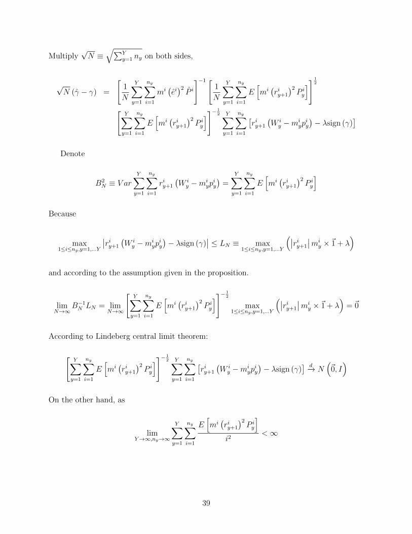
Multiply√N ≡

√∑Yy=1 ny on both sides,

√N (γ − γ) =

[1

N

Y∑y=1

ny∑i=1

mi(ei)2P i

]−1 [1

N

Y∑y=1

ny∑i=1

E[mi(riy+1

)2P iy

]] 12

[Y∑y=1

ny∑i=1

E[mi(riy+1

)2P iy

]]− 12 Y∑y=1

ny∑i=1

[riy+1

(W iy −mi

ypiy

)− λsign (γ)

]Denote

B2N ≡ V ar

Y∑y=1

ny∑i=1

riy+1

(W iy −mi

ypiy

)=

Y∑y=1

ny∑i=1

E[mi(riy+1

)2P iy

]

Because

max1≤i≤ny ,y=1,...Y

∣∣riy+1

(W iy −mi

ypiy

)− λsign (γ)

∣∣ ≤ LN ≡ max1≤i≤ny ,y=1,...Y

(∣∣riy+1

∣∣miy ×~1 + λ

)

and according to the assumption given in the proposition.

limN→∞

B−1N LN = lim

N→∞

[Y∑y=1

ny∑i=1

E[mi(riy+1

)2P iy

]]− 12

max1≤i≤ny ,y=1,...Y

(∣∣riy+1

∣∣miy ×~1 + λ

)= ~0

According to Lindeberg central limit theorem:

[Y∑y=1

ny∑i=1

E[mi(riy+1

)2P iy

]]− 12 Y∑y=1

ny∑i=1

[riy+1

(W iy −mi

ypiy

)− λsign (γ)

] d−→ N(~0, I)

On the other hand, as

limY→∞,ny→∞

Y∑y=1

ny∑i=1

E[mi(riy+1

)2P iy

]i2

<∞

39

according to Kolmogorov strong form law of large numbers, we have

1

N

Y∑y=1

ny∑i=1

mi(riy+1

)2P iya.s.−−→ 1

N

Y∑y=1

ny∑i=1

E[mi(riy+1

)2P iy

]

Therefore, based on the limit of the two parts of the product, we have

√N (γ − γ)

d−→ N

0,

[1

N

Y∑y=1

ny∑i=1

E[mi(riy+1

)2P iy

]]−1

from which we can conclude that γ is a consistent estimator of γ.

40

Table 1.1: Text Processing Working SampleThis paragraph is extracted from the MD&A section in the 2014 10-K of Apple Inc.. Original MD&A areextracted from 10-K files using regular expression matching. Tokens are generated in 5 steps: 1. EliminateHTML markups; 2. Downcase all letters (e.g. convert A-Z to a-z); 3. Separate letter strings from othertypes of sequences; 4. Delete strings not a letter, digit, $ or %; 4. Map numerical strings to #; 5. Clean upwhitespace, leaving only one white space between tokens. The McDonald financial English word dictionaryis used to filter out tokens that are not an English word.

Original MD&A The year-over-year growth in iPhone net sales and unit sales in2014 resulted primarily from the successful introduction of newiPhones in the latter half of calendar year 2013, the successfullaunch of iPhone 6 and 6 Plus beginning in September 2014, andexpanded distribution. iPhone unit sales grew in all of theCompany’s operating segments, while iPhone net sales grew in allsegments except Rest of Asia Pacific.

Tokenization the year over year growth in iphone net sales and unit sales in #resulted primarily from the successful introduction of new iphonesin the latter half of calendar year # the successful launch ofiphone # and # plus beginning in september # and expandeddistribution iphone unit sales grew in all of the company soperating segments while iphone net sales grew in all segmentsexcept rest of asia pacific

Dictionary Filtration year over year growth iphone net sales unit sales resultedprimarily successful introduction new iphones latter half calendaryear successful launch iphone plus beginning september expandeddistribution iphone unit sales grew all company operatingsegments while iphone net sales grew all segments except rest asiapacific

Table 1.2: Text Sample SizeThis table shows the number of document observations in each step. Full 10-K are original 10-K filesdirectly downloaded from SEC-Edgar database. MD&A are the Management Discussion and Analysissections extracted from 10-K files. Processed are MD&A files that are successfully processed using NLP tools(tokenization and dictionary filtration). Matched to Compustat and CRSP are files that can be matched tothe CRSP-Compustat merged dataset using CIK and filing date.

Source/Filter Sample size

Full 10-K 98805MD&A 96973

Processed 72437Matched to Compustat and CRSP 50940

41

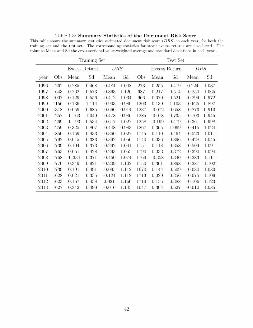
Table 1.3: Summary Statistics of the Document Risk ScoreThis table shows the summary statistics estimated document risk score (DRS) in each year, for both thetraining set and the test set. The corresponding statistics for stock excess returns are also listed. Thecolumns Mean and Sd the cross-sectional value-weighted average and standard deviations in each year.

Training Set Test Set

Excess Return DRS Excess Return DRS

year Obs Mean Sd Mean Sd Obs Mean Sd Mean Sd

1996 262 0.285 0.468 -0.484 1.008 273 0.255 0.419 0.224 1.0371997 643 0.262 0.573 -0.363 1.126 687 0.217 0.514 -0.250 1.0651998 1007 0.129 0.556 -0.412 1.034 966 0.070 0.521 -0.294 0.9721999 1156 0.136 1.114 -0.903 0.980 1203 0.139 1.103 -0.625 0.8972000 1318 0.059 0.685 -0.660 0.914 1237 -0.072 0.658 -0.873 0.9102001 1257 -0.163 1.049 -0.478 0.986 1285 -0.078 0.735 -0.703 0.9452002 1269 -0.193 0.534 -0.617 1.027 1258 -0.199 0.479 -0.361 0.9982003 1259 0.325 0.807 -0.448 0.983 1267 0.365 1.069 -0.415 1.0242004 1850 0.159 0.433 -0.360 1.027 1745 0.110 0.464 -0.523 1.0112005 1792 0.045 0.383 -0.392 1.056 1740 0.036 0.396 -0.428 1.0452006 1739 0.104 0.373 -0.292 1.041 1751 0.118 0.358 -0.504 1.0912007 1763 0.051 0.428 -0.293 1.055 1790 0.033 0.372 -0.390 1.0942008 1768 -0.334 0.371 -0.460 1.074 1769 -0.358 0.340 -0.283 1.1112009 1770 0.349 0.921 -0.209 1.102 1750 0.361 0.898 -0.287 1.1022010 1739 0.191 0.491 -0.095 1.112 1670 0.144 0.509 -0.080 1.0802011 1628 0.021 0.335 -0.124 1.112 1713 0.029 0.356 -0.075 1.1092012 1623 0.167 0.438 0.021 1.166 1719 0.155 0.388 -0.106 1.1232013 1627 0.342 0.490 -0.016 1.145 1647 0.304 0.527 -0.010 1.085

42

Table 1.4: Summary Statistics of the Tertile Portfolios Sorted on DRSIn each year, stocks are sorted into tertiles according to DRS. Tertile 1 contains stocks with lowest DRSand tertile 3 contains stocks with highest DRS. The last row 3-1 represents the factor mimicking portfoliowhich is constructed by longing tertile 3 and shorting tertile 1. The portfolio excess return for each quintileis calculated as the value-weighted average of excess returns of the component stocks. Monthly and yearlyexcess returns are accumulated daily excess returns. Each column Mean reports excess returns for eachtertile portfolio averages over the sample period, and each column S.d reports standard deviations of theexcess returns. Turnover is calculated as the percentage of stocks from a tertile portfolio in the next year,and Average turnover is the yearly turnover rates averaged over the sample period. The sample period isfrom 1996-2013.

Panel A: Yearly Returns of the DRS Tertiles

DRSYear TXT Low Medium High

1996 0.011 0.171 0.336 0.1881997 -0.094 0.277 0.287 0.1751998 0.067 -0.056 0.119 0.0201999 0.033 0.061 0.048 0.1152000 0.281 -0.192 -0.035 0.0632001 -0.192 0.051 -0.126 -0.1502002 -0.154 -0.123 -0.153 -0.2592003 0.143 0.305 0.322 0.4872004 0.041 0.100 0.121 0.1452005 0.022 0.023 0.034 0.0472006 0.008 0.123 0.125 0.1322007 0.174 -0.085 0.072 0.0832008 0.107 -0.435 -0.367 -0.3472009 0.245 0.142 0.338 0.4392010 0.007 0.180 0.136 0.1952011 0.065 0.004 0.015 0.0722012 -0.029 0.165 0.176 0.1312013 0.028 0.297 0.290 0.337

Panel B: Average Returns for the DRS Tertiles

Daily Monthly YearlyDRS Mean S.d. Mean S.d. Mean S.d.

Low 0.024 1.344 0.448 5.240 5.604 18.702Medium 0.038 1.243 0.752 4.756 9.662 18.908

High 0.040 1.291 0.812 5.308 10.409 20.998TXT 0.016 0.711 0.338 3.014 4.249 12.178

43

Table 1.5: Factor Correlations and Auto-correlationsPanel A shows the correlation between the five risk factors in monthly frequency. TXT is the factor mimickingportfolio constructed by longing the DRS-sorted tertile portfolio with highest document measured risk DRSand shorting the tertile portfolio with the lowest DRS. MKT is the market aggregate return. SMB is themimicking portfolio for the size risk and HML is the mimicking portfolio for the book-to-market risk in theFama and French (1993) 3-factor model. UMD is the mimicking portfolio for the momentum risk constructedby Kenneth French. The sample period is 1996-2013. Panel B reports the monthly factor mimicking portfolioaverage returns, standard deviation and their first-, second- and third-order auto correlations.

Panel A: Cross-Factor Correlations

TXT MKT SMB HML UMD

TXT 1.000 0.048 0.155 -0.176 -0.068MKT 0.048 1.000 0.239 -0.242 -0.324SMB 0.155 0.239 1.000 -0.176 0.067HML -0.176 -0.242 -0.176 1.000 -0.078UMD -0.068 -0.324 0.067 -0.078 1.000

Panel B: Factor Auto-correlations

Auto-correlationsMean S.d. Lag-1 Lag-2 Lag-3

TXT 0.338 3.014 0.039 -0.044 0.063MKT 0.582 4.682 0.113 -0.036 0.067SMB 0.270 3.354 -0.053 0.028 -0.093HML 0.303 3.402 0.109 0.005 0.100UMD 0.560 5.458 0.038 -0.098 0.081

44

Table 1.6: Characteristics of Value-Weighted PortfoliosValue-weighted quintile portfolios are formed every month by regression excess individual returns on TXT ,controlling for MKT , SMB, HML and UMD, using daily data over the previous month. TXT is thefactor mimicking portfolio for the text-implied risk. MKT is the aggregate stock returns. SMB and HMLare factor mimicking portfolios for the risks captured by size and book-to-market in the Fama-French (1993)three-factor model. UMD is the momentum factor constructed by Kenneth French. Stocks are sorted intoquintiles based on the coefficient βTXT from lowest (quintile 1) to highest (quintile 5). The column ExcessReturn are measured in monthly percentage terms. The Alpha columns report Jensen’s alpha with respectto the CAPM and Fama-French (1993) three-factor model (in percentage). Pre-Formation βTXT refers tothe value-weighted βTXT within each quintile portfolio estimated using daily data in the previous month.Post-Formation βTXT refers to the value-weighted βTXT within each quintile portfolio using daily data in thecurrent month. The reported pre-formation βTXT and post-formation βTXT for each portfolio are averagedacross the whole sample periods. The chunk with title Full Sample report the ex-post five factor loadings overthe whole sample. The ex-post betas are estimated by running a five-factor regression. Robust Newey-West(1987) t-statistics are reported in square brackets. The sample period is from February 1996 to December2013.

Excess Sharpe Pre-Formaton Post-Formation CAPM FF-3 Full SampleRank Return Ratio βTXT βTXT Alpha Alpha βMKT βSMB βHML βUMD βTXT

1 0.501 0.097 -1.221 -0.189 0.032 0.022 1.032 0.008 0.010 -0.059 -0.1160.262 0.186 29.291 0.238 0.209 -1.951 -2.650

2 0.445 0.101 -0.509 -0.102 0.046 0.039 0.897 -0.130 0.077 -0.018 0.0320.463 0.405 39.151 -3.281 1.530 -0.649 0.896

3 0.564 0.122 -0.002 -0.015 0.142 0.119 0.982 -0.073 0.099 0.053 -0.0181.194 1.068 28.875 -2.007 2.774 2.346 -0.387

4 0.828 0.178 0.511 0.088 0.410 0.343 0.959 -0.052 0.201 0.056 0.1103.292 3.187 33.603 -1.104 3.488 2.804 3.026

5 0.865 0.133 1.261 0.274 0.349 0.358 1.092 -0.034 -0.006 -0.007 0.1901.785 1.645 33.368 -0.702 -0.140 -0.178 3.731

5-1 0.364 0.087 0.337 0.326 0.078 -0.021 0.040 0.022 0.0102.180 2.128 2.040 1.515 -0.289 0.588 0.561 0.140

45

Table 1.7: Cross-sectional RegressionThis table reports the Fama and MacBeth (1973) factor premiums on Fama-French 5 × 5 portfolios two-way sorted on size and book-to-market. MKT is the excess return on the market portfolio, SMB is thesize factor and HML is the book-to-market factor in Fama and French (1993) 3-factor model . UMD isthe momentum factor constructed by Kenneth French. RMW is the profitability factor and CMA is theinvestment factor in Fama and French (2015) 5-factor model.

CAPM FF-3 FF-3 + UMD FF-5 FF-5 + UMDI II I II I II I II I II

Intercept 0.114 0.135 0.093 0.123 0.090 0.115 0.094 0.119 0.072 0.0964.501 4.284 3.190 4.257 2.207 3.026 3.107 3.944 2.112 2.966

MKT 0.068 0.090 0.053 0.088 0.050 0.080 0.051 0.081 0.029 0.0572.628 2.749 1.837 2.980 1.218 2.066 1.733 2.641 0.834 1.714

TXT 0.032 0.131 0.129 0.096 0.0830.967 2.385 2.279 1.992 1.758

SMB 0.007 0.009 0.008 0.009 0.009 0.010 0.010 0.0111.655 2.208 1.604 2.180 2.318 2.763 2.548 3.115

HML 0.012 0.010 0.012 0.010 0.017 0.015 0.019 0.0172.280 1.993 2.220 1.926 3.094 2.893 3.376 3.314

UMD 0.017 0.014 0.043 0.0410.200 0.184 3.947 4.121

RMW 0.039 0.015 -0.051 -0.0440.043 0.037 -2.448 -2.305

CMA 0.068 0.089 0.077 0.0742.136 3.697 1.041 1.116

R2adj 0.198 0.204 0.278 0.418 0.242 0.390 0.497 0.575 0.513 0.607

46

Table 1.8: TXT and Market IndexesThis table reports the time-series regression results of month-to-month percentage changes in market indexeson TXT and the controlling risk factors. VIX is the CBOE volatility index. Oil VIX is the CBOE crudeoil ETF volatility index. China VIX is the CBOE China ETF volatility index. S&P VIX is the CBOES&P 500 3-Month volatility index. Treasury VIX is the CBOE 10-Year Treasury Note Volatility Futures.Emerging Market VIX is the CBOE Emerging Markets ETF Volatility Index. Gold VIX is the CBOE GoldETF Volatility Index. Robust t-statistics with Newey and West (1987) standard errors are reported. Theperiod covered is 1996 – 2013 for VIX, Jan 2008 – Dec 2013 for S&P 3-Month VIX, Feb 2003 – Dec 2013 forTreasury VIX, Jun 2007 – Dec 2013 for Oil VIX, Jul 2008 – Dec 2013 for Gold VIX, Apr 2011 – Dec 2013for Emerging Market VIX, Apr 2011 – Dec 2013 for China VIX.

S&P 3-Month Treasury Oil Gold Emerging ChinaVIX VIX VIX VIX VIX Market VIX VIX

TXT -1.186 -2.196 -1.004 -1.444 -2.453 -2.263 -1.992t-stat -2.508 -2.620 -2.333 -2.773 -1.571 -3.435 -1.480R2adj 0.055 0.116 0.031 0.062 0.030 0.102 0.024

MKT -2.139 -1.938 -0.935 -1.129 -2.443 -1.279 -1.980t-stat -7.127 -3.992 -4.419 -3.374 -3.783 -3.804 -2.967R2adj 0.326 0.418 0.107 0.178 0.270 0.157 0.242

SMB -1.314 -1.939 0.066 -0.749 -3.080 -1.127 -2.603t-stat -2.971 -1.774 0.142 -1.073 -1.346 -1.210 -1.230R2adj 0.059 0.072 -0.008 0.004 0.060 0.013 0.059

HML 0.323 -0.724 -0.421 -0.571 -3.331 -0.141 -2.549t-stat 1.119 -0.706 -0.556 -0.885 -1.905 -0.138 -1.489R2adj -0.001 0.002 -0.001 0.000 0.045 -0.015 0.030

UMD 0.597 0.792 0.545 0.683 1.154 0.706 1.047t-stat 2.873 2.424 4.022 7.785 2.154 6.055 2.389R2adj 0.030 0.069 0.038 0.069 0.001 0.037 0.005

Obs 216 72 131 79 67 33 33

47

Table 1.9: TXT and Commodity PricesThis table reports the time-series regression results of month-to-month percentage changes in commodityprices on TXT and the controlling risk factors. Oil price is quoted from West Texas Intermediate (WTI).Natural Gas price is quoted from Henry Hub, LA. Gold price is the gold fixing price 10:30am (London time)in London Bullion Market, based in U.S. Dollars. Robust t-statistics with Newey and West (1987) standarderrors are reported. The period covered is from 1996 – 2013 for Oil and Gold, and 1997-2013 for Gas.

Oil Gas Gold

TXT 0.118 0.844 -0.017t-stat 0.601 2.757 -0.311R2adj -0.002 0.045 -0.004

MKT 0.183 0.089 -0.105t-stat 1.033 0.481 -1.882R2adj 0.006 -0.004 0.011

SMB 0.290 0.155 0.041t-stat 2.579 0.596 0.328R2adj 0.009 -0.004 -0.003

HML -0.045 -0.302 -0.097t-stat -0.211 -0.839 -1.142R2adj -0.004 0.001 0.002

UMD 0.014 0.068 0.042t-stat 0.102 0.328 0.905R2adj -0.005 -0.004 -0.001

Obs 216 204 216

48

Table 1.10: TXT and Market IndexesThis table reports the time-series regression results of month-to-month percentage changes in exchange rateson TXT and the controlling risk factors. Dollar index is trade weighted U.S. dollar index: major currencies(TWEXMMTH). Robust t-statistics with Newey and West (1987) standard errors are reported. The periodcovered is 1999 – 2013 for EURO, and 1996 – 2013 for other currencies.

Dollar Index EURO POUND YEN CAD YUAN

TXT -0.055 0.093 0.035 0.024 -0.104 -0.001t-stat -2.296 1.974 0.856 0.376 -2.772 -0.234R2adj 0.021 0.013 -0.001 -0.004 0.038 -0.004

MKT -0.080 0.121 0.087 0.034 -0.128 0.002t-stat -3.175 2.292 1.803 0.662 -2.795 0.592R2adj 0.087 0.046 0.034 -0.001 0.106 -0.003

SMB -0.042 0.046 -0.049 0.047 -0.099 0.005t-stat -1.364 0.749 -1.191 0.720 -2.959 1.208R2adj 0.008 -0.002 0.002 -0.001 0.029 -0.002

HML 0.003 0.024 0.021 0.108 0.010 0.003t-stat 0.096 0.332 0.516 1.846 0.251 0.972R2adj -0.005 -0.005 -0.003 0.016 -0.004 -0.003

UMD 0.039 -0.039 -0.027 -0.011 0.059 0.000t-stat 2.157 -1.048 -1.205 -0.335 2.218 0.036R2adj 0.025 0.003 0.001 -0.004 0.028 -0.005

Obs 216 180 216 216 216 216

49

Tab

le1.

11:

Most

Fre

quent

Word

sT

his

tab

lesh

ows

the

20m

ost

freq

uen

tw

ord

sin

the

MD

&A

docu

men

tsin

the

wh

ole

sam

ple

inea

chye

ar.

1995

1996

1997

1998

1999

2000

2001

2002

2003

1sa

les

sale

ssa

les

sale

sin

tere

stin

tere

stin

tere

stin

tere

stin

tere

st2

incr

ease

din

crea

sed

incr

ease

din

com

esa

les

sale

ssa

les

sale

sfinan

cial

3in

com

ein

com

ein

com

ein

crea

sed

inco

me

inco

me

inco

me

inco

me

inco

me

4in

crea

sein

crea

sein

crea

seop

erat

ions

oper

atio

ns

incr

ease

incr

ease

finan

cial

sale

s5

inte

rest

inte

rest

oper

atio

ns

incr

ease

incr

ease

din

crea

sed

incr

ease

dop

erat

ions

oper

atio

ns

6op

erat

ions

oper

atio

ns

inte

rest

inte

rest

incr

ease

oper

atio

ns

oper

atio

ns

asse

tsca

sh7

oper

atin

gco

mpar

edex

pen

ses

finan

cial

finan

cial

ended

cash

cash

asse

ts8

com

par

edduri

ng

oper

atin

gop

erat

ing

oper

atin

gex

pen

ses

pro

duct

sin

crea

seco

sts

9duri

ng

oper

atin

gre

venues

exp

ense

sco

sts

finan

cial

ended

pro

duct

sin

crea

se10

cash

exp

ense

sca

shpro

duct

sca

shca

shex

pen

ses

oper

atin

gop

erat

ing

11co

sts

cash

pro

duct

sen

ded

pro

duct

sop

erat

ing

oper

atin

gco

sts

pro

duct

s12

exp

ense

sre

venues

ended

reve

nues

exp

ense

spro

duct

sfinan

cial

incr

ease

dra

te13

pri

mar

ily

cost

sduri

ng

cash

ended

reve

nues

reve

nues

busi

nes

sen

ded

14finan

cial

pri

mar

ily

pri

mar

ily

cost

sre

sult

sco

sts

rate

exp

ense

sre

sult

s15

capit

alfinan

cial

com

par

edpri

mar

ily

reve

nues

rate

cost

sre

venues

rela

ted

16re

venues

appro

xim

atel

yco

sts

resu

lts

rate

pri

mar

ily

pri

mar

ily

resu

lts

exp

ense

s17

appro

xim

atel

yca

pit

alfinan

cial

duri

ng

busi

nes

sre

sult

sduri

ng

ended

mar

ket

18ra

tepro

duct

sap

pro

xim

atel

yco

mpar

edpri

mar

ily

duri

ng

resu

lts

mar

ket

busi

nes

s19

tota

lto

tal

capit

alsu

chsy

stem

sco

mpar

edco

mpar

edra

tein

crea

sed

20pro

duct

sen

ded

resu

lts

appro

xim

atel

yduri

ng

busi

nes

sm

arke

tduri

ng

duri

ng

50

Tab

le1.

12:

Most

Fre

quent

Word

s-

Conti

nue

Th

ista

ble

show

sth

e20

mos

tfr

equ

ent

wor

ds

inth

eM

D&

Ad

ocu

men

tsin

the

wh

ole

sam

ple

inea

chye

ar.

2004

2005

2006

2007

2008

2009

2010

2011

2012

1in

tere

stin

tere

stin

com

ein

com

ein

com

efinan

cial

inco

me

inco

me

inco

me

2sa

les

inco

me

inte

rest

inte

rest

inte

rest

inco

me

inte

rest

inte

rest

inte

rest

3in

com

esa

les

sale

sfinan

cial

finan

cial

inte

rest

finan

cial

cash

cash

4finan

cial

finan

cial

finan

cial

sale

sca

shca

shca

shfinan

cial

finan

cial

5ca

shca

shin

crea

sein

crea

sein

crea

sesa

les

sale

ssa

les

sale

s6

oper

atio

ns

incr

ease

cash

cash

sale

sop

erat

ions

oper

atio

ns

oper

atio

ns

incr

ease

7in

crea

seop

erat

ions

oper

atio

ns

oper

atio

ns

oper

atio

ns

asse

tsva

lue

incr

ease

oper

atio

ns

8co

sts

cost

sco

sts

cost

sta

xin

crea

seas

sets

ended

ended

9op

erat

ing

oper

atin

gin

crea

sed

incr

ease

das

sets

valu

een

ded

tax

tax

10pro

duct

spro

duct

sop

erat

ing

asse

tsco

sts

tax

tax

asse

tsop

erat

ing

11as

sets

asse

tsas

sets

ended

valu

eco

sts

oper

atin

gop

erat

ing

asse

ts12

rate

incr

ease

dra

teop

erat

ing

ended

ended

incr

ease

valu

eva

lue

13busi

nes

sra

teen

ded

tax

incr

ease

dop

erat

ing

cost

sre

late

dco

sts

14in

crea

sed

busi

nes

sre

late

dre

late

dre

late

dre

late

dre

late

dco

sts

rela

ted

15re

venue

rela

ted

tax

rate

oper

atin

gra

tera

tera

tera

te16

rela

ted

ended

exp

ense

sst

ock

rate

mar

ket

duri

ng

reve

nue

reve

nue

17re

sult

sre

venue

reve

nue

valu

ere

venue

busi

nes

sm

arke

tbusi

nes

sbusi

nes

s18

mar

ket

exp

ense

sduri

ng

bas

edbas

edduri

ng

busi

nes

sto

tal

tota

l19

ended

mar

ket

bas

edsp

acer

stock

reve

nue

reve

nue

duri

ng

incr

ease

d20

exp

ense

sduri

ng

tota

lex

pen

ses

busi

nes

sbas

edco

mpar

edm

arke

tco

mpar

ed

51

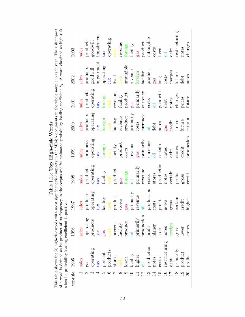
Tab

le1.

13:

Top

Hig

h-r

isk

Word

sT

his

tab

lesh

ows

the

20h

igh

-ris

kw

ord

sw

ith

most

sign

ifica

nt

risk

imp

act

sin

the

MD

&A

docu

men

tsin

the

wh

ole

sam

ple

inea

chye

ar.

Th

eri

skim

pact

ofa

wor

dis

defi

ned

asit

sp

rodu

ctof

its

freq

uen

cyin

the

corp

us

an

dit

ses

tim

ate

dp

rob

ab

ilit

ylo

ad

ing

coeffi

cien

tγj.

Aw

ord

class

ified

as

hig

h-r

isk

wh

enit

sp

rob

abilit

ylo

adin

gco

effici

ent

isp

osit

ive.

topru

le19

9519

9619

9719

9819

9920

0020

0120

0220

03

1sa

les

sale

ssa

les

sale

ssa

les

sale

ssa

les

sale

ssa

les

2ga

sop

erat

ing

pro

duct

spro

duct

spro

duct

spro

duct

spro

duct

spro

duct

spro

duct

s3

oper

atin

gpro

duct

sop

erat

ing

oper

atin

gop

erat

ing

oper

atin

gop

erat

ing

goodw

ill

goodw

ill

4ta

xta

xta

xta

xta

xta

xta

xim

pai

rmen

tim

pai

rmen

t5

per

cent

gas

faci

lity

faci

lity

fore

ign

fore

ign

fore

ign

oper

atin

gta

x6

pro

duct

sca

shca

shca

shca

shca

shca

shta

xop

erat

ing

7st

ores

per

cent

pro

duct

pro

duct

faci

lity

faci

lity

reve

nue

live

dca

sh8

cash

faci

lity

stor

esga

spro

duct

reve

nue

faci

lity

cash

reve

nue

9lo

wer

pro

duct

gas

fore

ign

cost

spro

duct

pro

duct

inta

ngi

ble

fore

ign

10fa

cility

oil

pri

mar

ily

oil

reve

nue

pri

mar

ily

gas

reve

nue

faci

lity

11hig

her

pri

mar

ily

reve

nue

pri

mar

ily

gas

cost

spri

mar

ily

fore

ign

gas

12oi

lpro

duct

ion

oil

reve

nue

pri

mar

ily

curr

ency

curr

ency

faci

lity

pro

duct

13pro

duct

ion

pro

fit

pro

duct

ion

cost

scu

rren

cyoi

lco

sts

pro

duct

inta

ngi

ble

14not

eshig

her

cost

sst

ores

oil

deb

toi

lga

sco

sts

15co

sts

cost

spro

fit

pro

duct

ion

cert

ain

not

esgo

odw

ill

long

live

d16

rest

ruct

uri

ng

not

esnot

esnot

esnot

esga

sdeb

tco

sts

oil

17deb

tfo

reig

ngr

oss

cert

ain

deb

tcr

edit

not

esch

arge

sdeb

t18

pri

mar

ily

gros

sce

rtai

npro

fit

stor

esst

ores

char

ges

futu

rere

stru

cturi

ng

19pro

duct

low

ercr

edit

gros

scr

edit

futu

repri

ces

deb

tnot

es20

pro

fit

stor

eshig

her

cred

itpro

duct

ion

cert

ain

futu

renot

esch

arge

s

52

Tab

le1.

14:

Top

Hig

h-r

isk

Word

s-

Conti

nue

Th

ista

ble

show

sth

e20

hig

h-r

isk

wor

ds

wit

hm

ost

sign

ifica

nt

risk

imp

act

sin

the

MD

&A

docu

men

tsin

the

wh

ole

sam

ple

inea

chye

ar.

Th

eri

skim

pact

ofa

wor

dis

defi

ned

asit

sp

rodu

ctof

its

freq

uen

cyin

the

corp

us

an

dit

ses

tim

ate

dp

rob

ab

ilit

ylo

ad

ing

coeffi

cien

tγj.

Aw

ord

class

ified

as

hig

h-r

isk

wh

enit

sp

rob

abilit

ylo

adin

gco

effici

ent

isp

osit

ive.

2004

2005

2006

2007

2008

2009

2010

2011

2012

1sa

les

sale

ssa

les

sale

sta

xta

xta

xta

xta

x2

pro

duct

spro

duct

sta

xta

xsa

les

sale

ssa

les

sale

ssa

les

3ta

xta

xop

erat

ing

oper

atin

gop

erat

ing

impai

rmen

tim

pai

rmen

tim

pai

rmen

tim

pai

rmen

t4

oper

atin

gop

erat

ing

pro

duct

spro

duct

sca

shop

erat

ing

oper

atin

gop

erat

ing

oper

atin

g5

impai

rmen

tim

pai

rmen

tca

shca

shpro

duct

sca

shca

shca

shca

sh6

goodw

ill

cash

impai

rmen

tga

sim

pai

rmen

tgo

odw

ill

goodw

ill

pro

duct

spro

duct

s7

cash

fore

ign

gas

reve

nue

reve

nue

pro

duct

sga

sfo

reig

nfo

reig

n8

reve

nue

reve

nue

reve

nue

impai

rmen

tga

sga

spro

duct

sgo

odw

ill

reve

nue

9fo

reig

nga

sfa

cility

faci

lity

fore

ign

reve

nue

fore

ign

reve

nue

gas

10ga

sfa

cility

fore

ign

fore

ign

faci

lity

fore

ign

reve

nue

gas

goodw

ill

11fa

cility

pro

duct

not

esnot

esoi

lfa

cility

faci

lity

fore

ign

oil

12pro

duct

goodw

ill

cost

soi

lgo

odw

ill

oil

oil

oil

faci

lity

13not

esnot

esoi

lpro

duct

not

esco

nte

nts

conte

nts

not

esnot

es14

oil

cost

spro

duct

cost

sse

gmen

tva

lue

not

esco

sts

conte

nts

15co

sts

oil

segm

ent

segm

ent

valu

ein

tangi

ble

segm

ent

segm

ent

segm

ent

16deb

tdeb

tgo

odw

ill

goodw

ill

cost

scr

edit

valu

edeb

tcr

edit

17fu

ture

segm

ent

deb

tre

late

dpro

duct

segm

ent

low

ercr

edit

deb

t18

segm

ent

futu

rere

late

ddeb

tre

late

dnot

escr

edit

futu

reva

lue

19ch

arge

sre

late

dcr

edit

valu

edeb

tfa

irdeb

tpri

ces

rela

ted

20re

late

dcu

rren

cypri

ces

conte

nts

conte

nts

deb

tnat

ura

lcu

rren

cyco

sts

53

Tab

le1.

15:

Top

Low

-ris

kW

ord

sT

his

tab

lesh

ows

the

20lo

w-r

isk

wor

ds

wit

hm

ost

sign

ifica

nt

risk

imp

act

sin

the

MD

&A

docu

men

tsin

the

wh

ole

sam

ple

inea

chye

ar.

The

risk

imp

act

ofa

wor

dis

defi

ned

asit

sp

rodu

ctof

its

freq

uen

cyin

the

corp

us

an

dit

ses

tim

ate

dp

rob

ab

ilit

ylo

ad

ing

coeffi

cien

tγj.

Aw

ord

class

ified

as

hig

h-r

isk

wh

enit

sp

rob

abilit

ylo

adin

gco

effici

ent

isn

egat

ive.

topru

le19

9519

9619

9719

9819

9920

0020

0120

0220

03

1in

tere

stlo

ans

inte

rest

inte

rest

inte

rest

inte

rest

inte

rest

inte

rest

inte

rest

2lo

ans

inte

rest

loan

slo

ans

loan

slo

ans

loan

slo

ans

loan

s3

loan

loan

loan

mor

tgag

eco

mpli

ant

loan

loan

loan

loan

4m

ortg

age

mor

tgag

em

ortg

age

loan

mor

tgag

em

ortg

age

mor

tgag

em

ortg

age

stock

5b

ank

ban

kban

kban

klo

anb

ank

stock

stock

mor

tgag

e6

dep

osit

sd

epos

its

stock

stock

ban

kst

ock

ban

kban

kse

curi

ties

7st

ock

stock

dep

osit

sd

epos

its

secu

riti

esse

curi

ties

secu

riti

esse

curi

ties

ban

k8

secu

riti

esse

curi

ties

secu

riti

esse

curi

ties

dep

osit

sdep

osit

sdep

osit

sdep

osit

sdep

osit

s9

sale

esta

teen

ded

ended

stock

ended

ended

loss

eslo

sses

10m

anag

emen

tre

alm

anag

emen

tm

anag

emen

ten

ded

inte

rnet

loss

esen

ded

acco

unti

ng

11es

tate

loss

essa

leco

mpli

ant

man

agem

ent

por

tfol

iop

ortf

olio

man

agem

ent

ended

12re

alsa

lees

tate

real

conti

nge

ncy

loss

eses

tate

sale

man

agem

ent

13d

eben

ture

sm

anag

emen

tre

ales

tate

read

ines

sre

alre

alac

counti

ng

por

tfol

io14

loss

esen

ded

loss

essa

lere

ales

tate

sale

por

tfol

iosa

le15

por

tfol

iob

eari

ng

shar

esp

ortf

olio

esta

tem

anag

emen

tm

anag

emen

tre

alre

al16

tota

lea

rnin

gco

mm

onlo

sses

por

tfol

iosa

lein

tern

etes

tate

esta

te17

dep

osit

por

tfol

iod

evel

opm

ent

com

mon

loss

esb

eari

ng

bea

ring

com

mon

issu

ed18

earn

ing

serv

icin

gse

rvic

ing

shar

essa

leea

rnin

gsh

ares

shar

esfin

19av

erag

ed

epos

itto

tal

dev

elop

men

tea

rnin

gco

mm

onco

mm

ondev

elop

men

tco

mm

on20

bea

rin

gto

tal

pro

ceed

sse

rvic

ing

shar

essh

ares

earn

ing

tota

lsh

ares

54

Tab

le1.

16:

Top

Low

-ris

kW

ord

s-

Conti

nue

Th

ista

ble

show

sth

e20

low

-ris

kw

ord

sw

ith

mos

tsi

gn

ifica

nt

risk

imp

act

sin

the

MD

&A

docu

men

tsin

the

wh

ole

sam

ple

inea

chye

ar.

The

risk

imp

act

ofa

wor

dis

defi

ned

asit

sp

rodu

ctof

its

freq

uen

cyin

the

corp

us

an

dit

ses

tim

ate

dp

rob

ab

ilit

ylo

ad

ing

coeffi

cien

tγj.

Aw

ord

class

ified

as

hig

h-r

isk

wh

enit

sp

rob

abilit

ylo

adin

gco

effici

ent

isn

egat

ive.

2004

2005

2006

2007

2008

2009

2010

2011

2012

1in

tere

stin

tere

stin

tere

stin

tere

stin

tere

stin

tere

stlo

ans

loan

slo

ans

2lo

ans

loan

slo

ans

loan

slo

ans

loan

sin

tere

stin

tere

stin

tere

st3

loan

loan

loan

mis

stat

emen

tslo

anlo

anlo

anlo

anlo

an4

mor

tgag

em

ortg

age

mor

tgag

elo

anst

ock

secu

riti

esse

curi

ties

secu

riti

esm

ortg

age

5st

ock

stock

stock

stock

secu

riti

esst

ock

mor

tgag

em

ortg

age

ban

k6

secu

riti

esse

curi

ties

ban

km

ortg

age

mor

tgag

em

ortg

age

ban

kst

ock

secu

riti

es7

ban

kb

ank

secu

riti

esse

curi

ties

ban

kb

ank

stock

ban

kst

ock

8d

epos

its

dep

osit

sd

epos

its

ban

kd

epos

its

dep

osit

sd

epos

its

dep

osit

sd

epos

its

9lo

sses

loss

eslo

sses

quan

tify

ing

loss

eslo

sses

loss

eslo

sses

loss

es10

por

tfol

iop

ortf

olio

por

tfol

iod

epos

its

por

tfol

iop

ortf

olio

esta

tees

tate

esta

te11

man

agem

ent

esta

teen

ded

loss

esen

ded

esta

tere

alre

alre

al12

end

edre

ales

tate

por

tfol

ioes

tate

real

por

tfol

iop

ortf

olio

por

tfol

io13

esta

teen

ded

real

end

edre

alen

ded

end

eden

ded

end

ed14

fin

man

agem

ent

man

agem

ent

real

man

agem

ent

man

agem

ent

man

agem

ent

man

agem

ent

man

agem

ent

15re

alsa

leac

cou

nti

ng

esta

tesa

led

epos

itd

epos

itd

epos

itd

epos

it16

sale

acco

unti

ng

sale

man

agem

ent

dep

osit

sale

com

mon

com

mon

com

mon

17ac

cou

nti

ng

tru

stto

tal

acco

unti

ng

acco

unti

ng

com

mon

sale

tota

lto

tal

18tr

ust

com

mon

dep

osit

sale

shar

esto

tal

tota

lsa

leb

ankin

g19

shar

essh

ares

tru

stfi

nco

mm

onsh

ares

bal

ance

shar

essh

ares

20co

mm

onto

tal

shar

esdep

osit

tota

lac

cou

nti

ng

shar

esb

ankin

gsa

le

55

Figure 1.1: Wordclouds of Word Risk ImpactsThe risk impact of a word is defined as the product of its frequency in the corpus and its estimated probabilityloading coefficient γj . A word classified as high-risk when its probability loading coefficient is positive, and aword classified as low-risk when its probability loading coefficient is negative. The left panel shows samplesof high-risk words with most significant impacts, and the right panel shows samples of low-risk words withmost significant impacts. Larger font size corresponds to words with larger impacts.

56

Figure 1.2: Histogram of Word Risk ImpactsThe risk impact of a word is defined as the product of its frequency in the corpus of the whole set and itsprobability loading coefficient γ. A word classified as high-risk when its probability loading coefficient ispositive, and a word classified as low-risk when its probability loading coefficient is negative. The left panelshows the histogram of log risk impacts of high-risk words, and the right panel shows the histogram of logrisk impacts of low-risk words.

57

Figure 1.3: Returns of the Market and Factor Mimicking PortfoliosThis figure shows the monthly excess returns of the aggregate market and factor mimicking portfolios,covering the period 1996 – 2013. TXT is the mimicking portfolio for the text-implied risk, which isconstructed by longing the tertile portfolio with highest DRS and shorting the tertile with lowest DRS.MKT is the market aggregate return. SMB is the mimicking portfolio for the size risk and HML is themimicking portfolio for the book-to-market risk from the Fama and French (1993) 3-factor model. UMD isthe mimicking portfolio for the momentum risk constructed by Kenneth French.

58

Figure 1.4: Accumulated Returns of the Market and Factor Mimicking PortfoliosThis figure shows the monthly excess returns of the aggregate market and factor mimicking portfolios,covering the period 1996 – 2013. TXT is the mimicking portfolio for the text-implied risk, which isconstructed by longing the tertile portfolio with highest DRS and shorting the tertile with lowest DRS.MKT is the market aggregate return. SMB is the mimicking portfolio for the size risk and HML is themimicking portfolio for the book-to-market risk from the Fama and French (1993) 3-factor model. UMD isthe mimicking portfolio for the momentum risk constructed by Kenneth French.

59

Chapter 2

Investment Manager Discussions and

Stock Returns

Abstract

This paper investigates whether the textual data in letters to shareholders written by

institutional investment managers contain valuable information that predicts future stock

returns. I quantify textual documents by mapping words and documents into a low

dimensional vector space using the continuous bag-of-words neural network model (Mikolov

et al. (2013a)). I then use the document vectors to predict value-weighted market portfolio

annual excess returns, controlling for past year returns and dividend yields. The

out-of-sample predictions using elastic-net show that the root mean square errors can be

reduced by about 6.6% when including textual features in the predicting model, and the

in-sample tests show that letters to shareholders contain information and the degree of risk

aversion of investors.

Key Words: information retrieval, market returns, text analysis, language modeling

JEL Classification: C11, C13, C45, C51, C52, D83, G12, G14, G17, G23

60

2.1 Introduction

In this paper, I investigate the relationship between investment manager discussions and

future expected stock returns. The question I try to answer is whether the information

delivered to investors by investment managers provides useful insights in predicting future

stock aggregate returns.

To answer my question, I construct a unique textual dataset which contains the letters

to shareholders written by investment managers. The letter to shareholders is part of the

semi-annual shareholder reports (N-CSR and N-CSRS1) that registered management

investment companies file with the Security and Exchange Commission (SEC). In these

letters, fund managers discuss macroeconomic environment, explain the constitutions of

their asset holdings and the related performance, compare the fund performance with

benchmarks and competing funds, as well as express opinions of future plans. Intuitively,

the forward-looking statements and subjective opinions of the investment professionals

contained in the letters may provide relevant information for the investors to understand

the concurrent investment conditions, or reflect sentiments of the investment managers.

To make statistical inferences using textual documents, I quantify the letters by

mapping words and documents into a low dimensional (relative to vocabulary size) vector

space using the continuous bag-of-words (CBOW) neural network model Mikolov et al.

(2013a)2. These vector representations for the words are called word embeddings. The

word embedding vectors are trained based on an unsupervised learning algorithm that tries

to predict a word based on its neighbors. In downstream prediction tasks, we need a vector

representation for each document, and a document vector is calculated as the average of

word vectors representing individual words appearing in the document. This approach of

1N-CSR and N-CSRS basically contained the same information. N-CSR is released at the end of afiscal year, while N-CSRS is released at the half-way of a fiscal year. They are treated in the same way inconstructing the letters to shareholders dataset.

2A related neural network model introduced in Mikolov et al. (2013b,a) is called Skip-Gram, while inCBOW, word vectors are trained based on unsupervised learning algorithm that tries to predict a wordbased on its neighbors; in Skip-gram, word vectors are trained to predict the surrounding words of a wordbased on a target word.

61

generating document vectors is referred as CBOW-Average. This is fundamentally different

from the word counting approach based on pre-built dictionaries that are commonly

applied in previous finance literature (Tetlock (2007), Loughran and McDonald (2011),

Jegadeesh and Wu (2013), etc.). The advantage of my approach is that it avoids the

subjectivity of human readers involved in building word classifying dictionaries, and it

quantifies documents in a systematic way such that it requires much less human labor and

can be applied to textual data of different domains.

The word embedding approach is drawing a great deal of attention from researchers in

computational linguistics in recent years. In comparison to the traditional bag-of-words

model, it generates superior results in many natural language processing (NLP) tasks such

as part of speeching tagging, sentiment analysis, speech recognition, etc. In a bag-of-words

model, words are treated as atomic units, without considering context information. In

comparison, the vector representations of words can capture the precise syntactic and

semantic word relationships. Distributed representations of words in a vector space help

learning algorithms to achieve better performance in natural language processing tasks by

grouping similar words.

To test the prediction power of the document vectors, I conduct out-of-sample (OOS)

predictions. The dependent variable is the annual stock return of the Center for Research

in Security Prices (CRSP) value-weighted market portfolio, which is calculated as the

accumulated return covering a 252-day period starting from the day following the

N-CSR(S) release date. The explanatory variables include two controlling variables, the

leading annual stock return of the market portfolio and the dividend yield of the market

portfolio.

The whole sample set include the 2,255 daily observations covering the period 2003-2015.

I construct a training set and a test set in two ways. First, I pool all the 2,255 observations

together ignoring their time stamp and randomly select 70% of the samples to form the

training set, and use the rest samples to build the test set. I estimated a linear model based

62

on the training set using elastic-net. Elastic-net is capable of dealing with high-dimension

explanatory variables as the penalization in the L1 and L2-norm of the coefficients could

reduce overfitting. I find that including the document vectors can reduce the OOS prediction

root mean square errors (RMSEs) significantly, by about 6.6%.

As constructing the training and test sets through random splitting may introduce looking

ahead bias as the training set contain future information in comparison to the test set.

Therefore, in the second way, I split the training and the test sets on rolling window basis. For

every 6-year window, I estimate the predicting model using the data in the leading five years

and make OOS predictions in the sixth year. In this approach, I still find that including the

document vectors in the prediction can still reduce the OOS prediction RMSEs significantly.

This rolling window based OOS predictions confirm that the letters to shareholders contain

substantial return predicting information.

Generally speaking, the CBOW neural network model can be considered as a kind of

dimension reduction technique that summarizes sparse information contained in documents

into a low-dimensional vector. However, it is not the only way to learn low dimensional

vector representations of words and documents. I compare the predictive power of

document vectors generated by CBOW-Average with six other language models:

CBOW-Doc, CBOW-Kmeans, CBOW-Spectral Clustering, Sentiment Counting, Latent

Semantic Analysis (LSA), and Latent Dirichlet Allocation (LDA). Through the

comparison, I find that CBOW-Average generates smallest OOS prediction RMSEs when

the training and test set are split in a rolling window basis, and CBOW-Doc generates

smallest OOS prediction RMSEs when the training and test set are split randomly.

In additional to stock returns, I also investigate the predicting power of textual features in

predicting stock return volatilities and the growth rates of oil price, dollar index, and default

spreads. I find that including the textual features into the model can reduce the OOS

prediction RMSEs significantly, in comparison to benchmark models without the textual

features.

63

Also, I investigate the economic meaning of the textual information that can predict

stock returns. As previous research in asset pricing suggest that the predictive part of stock

returns is risk premium, which is affected by the degree of risk aversion of a representative

investor. I construct two measures of risk aversion based on counting the frequency of words

that are related to investment uncertainties and business cycles. Notice that my approach

of classifying words is based on the semantic distance measured by the cosine similarity of

their embedding vectors learned based on CBOW, rather than human designed rules, which

is free of subjective judgment and is easy to be applied to a different corpus. I find that

my text-based risk aversion measure contains information in predicting stock returns. When

the proportion of investment uncertainty related words increase by 1%, the expected annual

stock returns increase by 5%, which is economically and statistically significant; and when

the proportion of business cycle related words increase by 1%, the expected annual stock

returns increase by 1%.

This paper is related to two strands of literature in finance. First, it is related to the

literature of stock return predictability. The predictability of stock returns has been under

debate for a long time (Campbell and Yogo (2006); Ang and Bekaert (2007); Cochrane

(2011); Fama and French (1988)). Now many financial economists agree that long-term

stock returns are predictable. In particular, the predictable part of stock returns is the risk

premium. As the risk aversion property of an investor is subjective in nature, the degree

of risk aversion is difficult to measure empirically. However, the textual data of letters

to shareholders, which reflect the subjective opinions of investment managers, provide a

unique source to measure risk aversion. Intuitively, the risk aversion nature of an investment

manager affects the information he/she puts into the letters to shareholders. I find we

can construct proxies that measure the risk aversion of investors to predict stock returns

by retrieving the textual information in the letters. In addition, I also find the investment

manager discussions contain information in predicting future stock return volatilities, as well

as some macroeconomic indicators. This results agrees with the previous literature about

64

stock return predictability such as Kogan et al. (2009).

Second, this paper is related to the literature about investment manager abilities. It has

been discussed for a long time whether fund managers have superior abilities to pick stocks or

to time the market and add value to their clients (Edwards and Caglayan (2001); Brands et al.

(2005); Cremers and Petajisto (2009)). Understanding how investment managers add value

is important because a significant and growing proportion of individual investors delegate

their portfolio management to investment professionals. Kacperczyk et al. (2014) found that

a small subset of funds persistently outperforms, due to their superior capabilities of picking

stocks in expansions and timing the market in recessions. The prerequisite for an investment

manager to outperform the market is to have insights about the market. My paper suggests

that as the information delivered to fund investors indeed contains valuable information to

predict market returns, it can be inferred that investment managers indeed have capabilities

to understand the market and make informative investments.

The remainder of this paper is organized as follows. Section 2 introduces the CBOW

neural network language model. Section 3 describes the dataset. Section 4 reports the main

empirical results. Section 5 discusses the economic interpretation of the predictability of the

document vectors. Section 6 concludes.

2.2 Language Model

Textual documents come to econometricians in the format as strings of words, and we have

to quantify the textual documents for downstream statistical analysis.

Many machine learning algorithms require the input to be represented as a fixed-length

feature vector. In textual analysis, one of the most common fixed-length features is bag-of-

words. Bag-of-words is popular because of its simplicity and surprising robustness in many

NLP applications. However, the bag-of-words model has two major weakness. First, the

order information of a word is lost, and thus two different sentences could have the same

65

representations. Although a derivation of the bag-of-words model, the bag-of-n-grams model

incorporates some local order information into the vector representation of a document,

it suffers from data sparsity and high dimensionality. Second, the semantic information

contained in a document is lost in a bag-of-words representation. For example, in a financial

report corpus, a pair of words like “stock” and “returns” should be semantically closer to

each other than a pair of words like “stock” and “China”, because “stock” and “returns”

are more likely to appear together. However, in a bag-of-words model, the three words are

equally distant from each other.

To overcome the shortcomings of the bag-of-words model, a collection of word embedding

models are proposed in the computational linguistic literature (Bengio et al. (2006); Collobert

and Weston (2008); Mnih and Hinton (2009); Turian et al. (2010); Mikolov et al. (2013b,a);

Tang et al. (2014)). The idea is to map words or phrases into a low dimensional (relative

to the vocabulary size) vector space such that semantic similarity between words can be

measured using vector distances.

2.2.1 CBOW

The CBOW word embedding model is a neural network model introduced by Mikolov et al.

(2013b). It provides an efficient method for learning high-quality vector representations of

words from large amounts of unstructured text data and has achieved great popularity in the

computational linguistic research. The idea of CBOW is to find word vector representations

that are useful for predicting a target word using surrounding words in a paragraph. The

architecture of CBOW is shown in Figure 2.1, which is essentially a convolutional neural

network. Each surrounding word as an input is mapped a word embedding vector, the

average of surrounding word vectors forms the context vector, based on which we predict

the target word.

More formally, using the notation in Levy and Goldberg (2014), Denote the vocabulary

set of words in a corpus as VW , and the set of contexts VC . In CBOW, the contexts for

66

word wt are the surrounding words in a window with length 2l:

ct = (wt−l, ..., wt−1, wt+1, ..., wt+l), containing l words ahead of wt, and l words following wt.

Denote D as the set of observed words and context pairs. Consider a word-context pair

(w, c), and let p(w∣∣c) be the probability that w appears in context c.

The idea of CBOW (and other word embedding models) is to associate each word w ∈ VW

with a vector vw ∈ Rr, and similarly associate each context c ∈ VC with a vector vc ∈ Rr,

where r is the embedding’s dimensionality, a hyper parameter chosen by researchers. The

elements in the vectors are latent parameters to be learned from the model. Denote # (w, c)

as the counts of the pair (w, c) in D, # (w) =∑

c′∈VC # (w, c′) and # (c) =∑

w′∈Vw # (w′, c)

as the counts of w and c in D, respectively.

In CBOW, the probability for a word w to appear in context c is modeled as a sigmoid

function of the inner product of the word vector and context vector

p(w∣∣c) = σ (vw · vc) ≡

1

1 + exp (−vw · vc).

The learning of CBOW employs the negative sampling technique, in which the objective for

a single (w, c) is to maximize the average log probability

log σ (vw · vc) + k · EcN∼P (c)σ (−vw · vcN ) .

The idea of the objective function is to maximize p(w∣∣c) for (w, c) that appears in the

corpus, while minimizing p(w∣∣cN) for (w, cN) not appearing in the corpus. k is the number

of “negative” samples. When k is large, the objective puts more weight on penalizing

unobserved (w, c) pairs; when k is small, the objectives puts more weight on maximizing

the likelihood of observed (w, c) pairs. cN denotes contexts drawn from the empirical

distribution P (c) = #(c)|D| , the proportion of observed context c in set D. The global

67

Figure 2.1: Architecture of CBOWThis figure demonstrates the neural network architecture of CBOW. Each word is mapped to a wordembedding vector. The context vector is the average of surrounding word vectors. The distribution ofa target word is determined by the inner product of its own embedding vector and the context vector.

objective is to maximize the sum of the objective of single (w, c) pairs:

L =∑w∈VW

∑c∈VC

# (w, c)1

T

T∑t=1

[log σ (vw · vc) +

k∑i=1

EcN∼P (c)σ (−vw · vcN )

].

CBOW-Average Training texts using CBOW only generates the embedding vectors for

each word, but we need an embedding vector for each document in training downstream

stock return prediction models. In CBOW-Average, a document vector is simply calculated

as the average of the word vectors corresponding to words in the document. Otherwise

explicitly specified, all the document vectors in this paper refer to vectors generated through

CBOW-Average.

CBOW-Doc CBOW-Doc (Le and Mikolov (2014)) is a derivation of the original CBOW

model, which directly encodes the co-occurrence of words and documents into the neural

network structure and directly estimates a document vector. In CBOW-Doc, not only each

word, but also each document is represented as a vector, and the probability for word w to

appear in context c and document d is

p(w∣∣c, d) = σ (vw · (αvc + (1− α) vd)) ,

68

Figure 2.2: Architecture of CBOW-DocThis figure demonstrates the neural network architecture of CBOW-Doc. Each word and document ismapped to a word embedding vector. The context vector is the average of surrounding word vectors. Thedistribution of a target word is determined by the inner product of its own embedding vector and a weightedaverage of the context vector and document vector.

where vd ∈ Rr is the vector representing document d, and α ∈ [0, 1] is the weight assigned

to the context vector vc in affecting word distributions. The architecture of the CBOW-Doc

model is shown in Figure 2.2.

2.2.2 Matrix Factorization

The specification of the CBOW neural network has an intuition of coercing words surrounded

by similar contexts to have similar embeddings. However, it does not provide intuition to

understand the meanings of the embeddings. Levy and Goldberg (2014) justifies that neural

word embedding can be considered as implicit word-context matrix factorization, and thus

each dimension of the embedding spaces represents as a hidden topic of the corpus.

General word embedding models starts with a word-context matrix M . The process of

learning word embedding vectors is to factorize the word-context matrix into a |VW |×r word

embedding matrix W and a |VC | × r context embedding matrix C such that M = W · C ′,

which embeds both words and their contexts into a low-dimensional space Rr. Each row

of W corresponds to a word, and each row of C corresponds to a context. Each element

Mwc = vw · vc measures the association between a word and a context.

Levy and Goldberg (2014) proved CBOW is essentially factorizing a word-context matrix

69

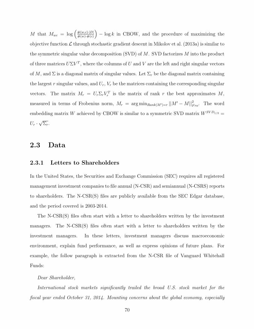
M that Mwc = log(

#(w,c)·|D|#(w)·#(c)

)− log k in CBOW, and the procedure of maximizing the

objective function L through stochastic gradient descent in Mikolov et al. (2013a) is similar to

the symmetric singular value decomposition (SVD) of M . SVD factorizes M into the product

of three matrices UΣV T , where the columns of U and V are the left and right singular vectors

of M , and Σ is a diagonal matrix of singular values. Let Σr be the diagonal matrix containing

the largest r singular values, and Ur, Vr be the matrices containing the corresponding singular

vectors. The matrix Mr = UrΣrVTr is the matrix of rank r the best approximates M ,

measured in terms of Frobenius norm, Mr = arg minRank(M ′)=r ||M ′ −M ||2Fro. The word

embedding matrix W achieved by CBOW is similar to a symmetric SVD matrix W SV D1/2 =

Ur ·√

Σr.

2.3 Data

2.3.1 Letters to Shareholders

In the United States, the Securities and Exchange Commission (SEC) requires all registered

management investment companies to file annual (N-CSR) and semiannual (N-CSRS) reports

to shareholders. The N-CSR(S) files are publicly available from the SEC Edgar database,

and the period covered is 2003-2014.

The N-CSR(S) files often start with a letter to shareholders written by the investment

managers. The N-CSR(S) files often start with a letter to shareholders written by the

investment managers. In these letters, investment managers discuss macroeconomic

environment, explain fund performance, as well as express opinions of future plans. For

example, the follow paragraph is extracted from the N-CSR file of Vanguard Whitehall

Funds:

Dear Shareholder,

International stock markets significantly trailed the broad U.S. stock market for the

fiscal year ended October 31, 2014. Mounting concerns about the global economy, especially

70

the threat of deflation in Europe and a slowdown in China and other emerging markets,

contributed to the weakness....

Sincerely,

F. William McNabb III

The SEC only provides general instructions on N-CSR(S) filing, but there is no strict

structured template for the companies to follow. Therefore, the structures of N-CSR(S)

files across firms are pretty heterogeneous, and there is no uniform boundaries between the

letters and the rest part of a file. This fact makes extracting a certain section from the

N-CSR(S) files much more challenging than extracting sections from well structured SEC

files like 10-Ks, the corporate annual reports.

I extract the letters to shareholders using regular expression matching. As there is no

separate section for letters to shareholders, I use the common letter starting words (e.g.

“Dear Shareholders”, “Letters to Shareholders”, “Fellow Shareholders”) to match the

beginning of a letter and use ending words (e.g.“Yours sincerely”, “Respectfully”,“Best

regards”) to match the end of a letter. Table 2.1 shows the counts of the original

N-CSR(S) files and the letters extracted from the original files, as well as the extraction

rate, the proportion of letters extracted from the original files successfully. The total

number of the N-CSR files is 37, 862, and the total number of letters extracted from the

N-CSR files is 21, 937, with average extraction rate of 0.58. The total number of N-CSRS

files is 31, 139, and the total number of letters extracted from the N-CSRS files is 15, 077,

with average extraction rate of 0.48.

After extracting the letters from the N-CSR(S) files, following Kogan et al. (2009), I

tokenize the letters in six steps: 1. Eliminate HTML markups; 2. Downcase all letters

(convert A-Z to a-z); 3. Separate letter strings from other types of sequences; 4. Delete

strings not a letter; 5. Clean up whitespace, leaving only one whitespace between tokens. 6.

Remove stopwords.

A paragraph of an example letter and its tokenized version are demonstrated in the Table

71

Table 2.1: Document counts and letter extraction ratesThis table shows the numbers of N-CSR(S) files and letters to shareholders extracted from those files in eachyear. The extraction rate is the proportion of letters extracted from the N-CSR(S) files.

N-CSR N-CSRS

Files Letters Extraction Rate Files Letters Extraction Rate

2003 2801 1527 0.55 984 460 0.472004 3968 2338 0.59 2615 1286 0.492005 3527 2154 0.61 2727 1415 0.522006 3361 1997 0.59 2738 1353 0.492007 3326 1967 0.59 2806 1248 0.442008 3293 1989 0.60 2787 1270 0.462009 3163 1938 0.61 2743 1345 0.492010 2927 1619 0.55 2772 1360 0.492011 2964 1652 0.56 2720 1393 0.512012 2832 1554 0.55 2742 1333 0.492013 2851 1583 0.56 2723 1307 0.482014 2849 1619 0.57 2782 1307 0.47

Total 37862 21937 0.58 31139 15077 0.48

2.6 in the Appendix, and the summary statistics for the length of the tokenized letters are

shown in Table 2.7 in the Appendix. We can see that the average length of a tokenized letter

contains about 500 words and the length varies a lot from letter to letter.

As multiple N-CSR(S) files may be filed on the same day, I concatenate the letters to

shareholders written by different investment managers on the same day together and treat it

as a single document. Because the my research question is to test whether a representative

investment manager has insights about market performance, there is no need to identify

individual managers. In addition,for CBOW, the word embedding vectors are learned based

on the co-occurrence of words in the same sentence, and thus the concatenation does not

impair the learning of the word embedding vectors. For CBOW-Doc, this may add bias to

the estimation of the word and document vectors as the concatenation procedure creates

some fake co-occurrence of some words and documents.

72

2.3.2 Stock Returns

The daily stock return data of the value-weighted market portfolio come from the Center for

Research in Security Prices (CRSP) dataset.

CRSP provides the market portfolio return data both including (vwretd) and excluding

(vwretx) dividends. Denote the price of the market portfolio at time t as Pt, and its dividend

as Dt. The market portfolio returns including and excluding dividends from period t− 1 to

t are vwretdt = (Pt +Dt) /Pt−1 − 1 and vwretxt = Pt/Pt−1 − 1 respectively. Therefore, the

dividend yield log (Dt/Pt) can be constructed as

dividend yieldt = log

(1 + vwretdt1 + vwretxt

− 1

).

To test whether the document vectors contains information in predicting the stock returns

of the market portfolio. I use the document vector at date t, to predict the annual excess

return of the market portfolio, which is calculated as the accumulated returns from t+ 1 to

t+ 252. The excess return is gross return (vwretd) minus the risk-free rate. The risk-free is

proxied by the interest rate of 3-Month Treasury Bills in this paper. The controlling variables

are dividend yieldt and return leadingt, where return leadingt is the leading annual stock

return of the value-weighted market portfolio, which is calculated as the accumulated returns

from t− 251 to t.

The value and momentum factors are two of the most popular pricing factors in the

asset pricing literature and are found to explain a significant proportion of variations in the

cross-section of stock returns (Fama and French (1993); Carhart (1997)). In the market

portfolio time series predictions, dividend yieldt captures value factor, and return leadingt

captures the momentum factor. They are found to have significant power in predicting

long-term stock returns (Lettau and Ludvigson (2001); Cochrane (2011); Fama and French

(1988)), and thus I include dividend yieldt and return leadingt in my predicting models as

a controlling variables.

73

2.4 Empirical Results

2.4.1 Word Vectors

I apply the CBOW model using the Python module Gensim (Rehurek and Sojka (2010)).

Gensim provides Python interface to the Word2Vec software of Google which originally

implemented the CBOW model. It is recommended to represent words in a relative

high-dimension vector space in literature (Mikolov et al. (2013b)) to achieve accurate word

embedding estimates. In practice, a common choice of the dimension is 150 − 400. In this

paper, I choose the embedding dimension to be 300 and length of the context window l to

be equal to 2, meaning the context of a word contains 2 leading and 2 following words.

Examples showing the top similar words to a few seed words are listed in Table 2.2. For

example, the top 10 words that have highest semantic similarity to the word “china” are

“chinese”, “indonesia”, “brazil”, “russia”, “japan”, etc., which is sensible as Indonesia and

Japan are countries geographically close to China, and Brazil, Russia, India are often referred

as Gold BRICS countries in financial documents. The topic 10 words that have closest

semantic similarity to the word “oil” are “commodity”, “energy”, “gasoline”, “cotton” etc.,

which is also reasonable because these words often appear together in letters to shareholders

written by investment managers that focus on commodity trading.

2.4.2 Word Clouds

The nonlinear dimension reduction technique t-SNE (Van der Maaten and Hinton (2008))

is a powerful dimension reduction method to project the high-dimension word vectors into

a low-dimension space such that we can visualize the word locations in a 2-d graph.

The visualization of some sentiment words are demonstrated in Figure 2.7 in the

Appendix. To generate the positive and negative word lists, I use the keywords “good” and

“bad” as seed words, and find 40 words that have the highest semantic similarity to them.

We can see the splitting between positive words like “good”, “excellent”, “superior” and

74

Table 2.2: Similar WordsThis table demonstrates the top 10 similar words to “china”, “oil”, “recession” and “shareholder”. Thesimilarity between 2 words are measured as the cosine similarity of their word embedding vectors.

china oil politics shareholder

1 chinese commodity terrorism shareholders2 indonesia energy rhetoric stockholders3 brazil gasoline political stockholder4 russia cotton standoff shareowner5 japan fuel presidential trustees6 asia gold partisan shareowners7 turkey brent debate classify8 states natural threats directors9 population food uncertainties mergers10 india ore attacks semiannual

negative words “bad”, “terrible”, “discouraging”, and words with the same sentiment are

close to each other.

The visualization of words classified by economic topics are demonstrated in Figure 2.8

in the Appendix. I include eight topics in the graph: regions, politics, macroeconomy,

market index, commodity, industry, investment and shareholder. To generate the word list

for each topic, I use the keywords “region”, “politics”, “macroeconomy”, “index”,

“commodity”, “industry”, “investment”, “shareholder” as seed words, and find 30 words

that have the highest semantic similarity to the seed word for each topic. For example, the

words having closest semantic meaning to “commodity” include “gold”, “oil”, “electricity”,

“copper” etc; the words having closest semantic meaning to “region” include “china”,

“japan”, “russian”, “asia” etc; the words having closest semantic meaning to “politics”

include “politicians”, “democracy”, “presidential”, “legislative” etc. The word lists agree

with our linguistic intuition.

The distributed location of the economic topic word clouds in Figure 2.8 also generate

intuitive results. First of all, words close to each other in semantic meaning indeed locate

close to each other. Second, topics that are supposed to have a close linguistic relationship

75

also locate close to each other. For example, in news articles or financial reports, people

often tie politics to a certain region, like wars in the mid-east or presidential elections in

the United States. In the words clouds, we indeed see the “politics” topic located close

to the “region” topic. When institutional investors make investments, the macroeconomic

condition is an important factor affecting their investment decisions, and the “macro” and

“investment” topic are indeed close to each other in the word clouds

2.4.3 Out-of-sample Predictions

For out-os-sample (OOS) predictions, I construct the training and test datasets in two ways,

random splitting and rolling window splitting.

Random Splitting For random splitting, I first pool all the 2,255 observations together,

and randomly select 70% of the observations to form the training set, and use the rest 30%

observations to form the test set. I consider five linear models, which include different

explanatory variables: (1). “Constant”, the explanatory variable include only a constant,

which is equivalent to prediction using training set mean; (2). “Mom”; the explanatory

variables include a constant and the momentum factor return leadingt; (3). “Mom&Val”,

the explanatory variables include a constant, the momentum factor return leadingt and

value variable dividend yieldt; (4). “CBOW-Average”; the explanatory variables include

the document vectors generated using the CBOW-Average model in addition to the

controlling variables in “Benchmark”; (5). “CBOW-Doc”, the explanatory variables

include the document vectors generated using the CBOW-Doc model in addition to the

controlling variables in “Benchmark”.

I estimate the linear models using elastic-net. The penalization parameter of the elastic-

net is selected through 10-fold cross validation. I measure of the prediction accuracy using

OOS RMSEs.

To reduce the random effect of the training-test set splitting, I follow a bootstrap approach

76

by repeating the training-test split 50 times. The OOS prediction RMSEs of the five models

are shown in Figure 2.3. In addition to 1-year returns, I also checked predicting power

of textual features on 1-month and 6-month returns (the corresponding momentum factor

return leadingt is adjusted accordingly). To make the results for returns of different horizons

comparison, I normalize the OOS RMSEs of the Const model to be equal to 1, and scale the

RMSEs generated by other models correspondingly. In the bar chart, the height of the bars

represent the average OOS RMSEs of the 50 experiments, and the standard errors are also

demonstrated through the error bars.

We can see that by including document vectors generated by CBOW-Average in the stock

return prediction model, we can reduce the OOS RMSEs by about 1.0% for 1-month returns,

4.2% for 6-month returns, and 6.6% for 1-year returns, in comparison to predicting using

training set mean. It means that the textual features generated by CBOW indeed contains

valuable information in predicting future stock returns, and the prediction power increases

with the length of horizon. The textual features generated by CBOW-Doc is more powerful

in predicting long-term stock returns, but it underperforms in predicting short-term returns.

Rolling Window Splitting One possible concern about the forecasting results presented

above is the potential “look-ahead” bias due to the fact the training set contains information

in the future. This concern can be addressed by forming the training and test set in a rolling

window basis and performing OOS forecasts where the parameters in the linear model are

re-estimated every period, using only data available at the time of the forecast.

I consider rolling windows with length equal to six years. In every window, I use

observations in the leading five years to form the training set to estimate the model

parameters, and make predictions in the sixth year to calculate the OOS RMSEs. The

RMSEs of the five models are shown in Table 2.3. As the data set covers the period

2003-2014, the first 6-year window is 2003-2008, and thus the RMSEs reported in the table

starts from the year 2008.

77

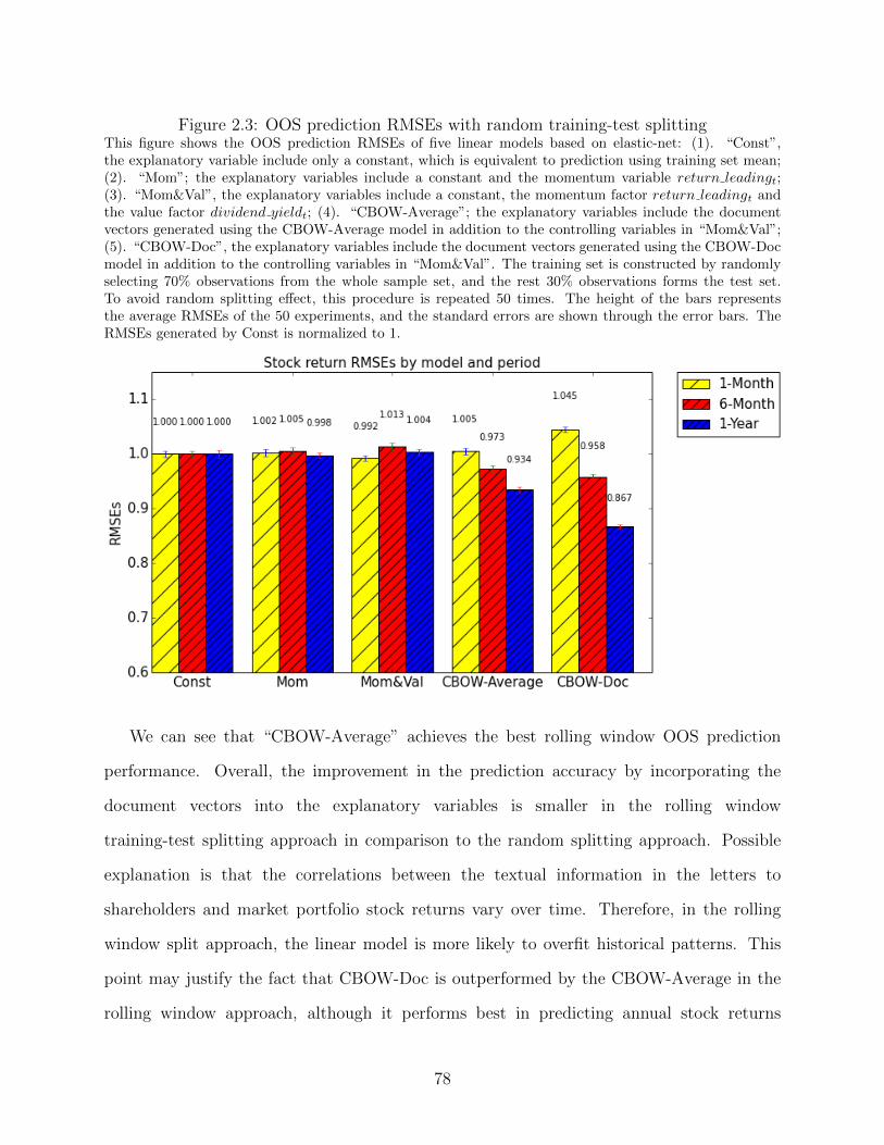
Figure 2.3: OOS prediction RMSEs with random training-test splittingThis figure shows the OOS prediction RMSEs of five linear models based on elastic-net: (1). “Const”,the explanatory variable include only a constant, which is equivalent to prediction using training set mean;(2). “Mom”; the explanatory variables include a constant and the momentum variable return leadingt;(3). “Mom&Val”, the explanatory variables include a constant, the momentum factor return leadingt andthe value factor dividend yieldt; (4). “CBOW-Average”; the explanatory variables include the documentvectors generated using the CBOW-Average model in addition to the controlling variables in “Mom&Val”;(5). “CBOW-Doc”, the explanatory variables include the document vectors generated using the CBOW-Docmodel in addition to the controlling variables in “Mom&Val”. The training set is constructed by randomlyselecting 70% observations from the whole sample set, and the rest 30% observations forms the test set.To avoid random splitting effect, this procedure is repeated 50 times. The height of the bars representsthe average RMSEs of the 50 experiments, and the standard errors are shown through the error bars. TheRMSEs generated by Const is normalized to 1.

We can see that “CBOW-Average” achieves the best rolling window OOS prediction

performance. Overall, the improvement in the prediction accuracy by incorporating the

document vectors into the explanatory variables is smaller in the rolling window

training-test splitting approach in comparison to the random splitting approach. Possible

explanation is that the correlations between the textual information in the letters to

shareholders and market portfolio stock returns vary over time. Therefore, in the rolling

window split approach, the linear model is more likely to overfit historical patterns. This

point may justify the fact that CBOW-Doc is outperformed by the CBOW-Average in the

rolling window approach, although it performs best in predicting annual stock returns

78

when we split the dataset into a training set and a test set randomly. Because the word

vectors built through CBOW-Average are solely based on co-occurrence of neighboring

words, which do not depend on document level information which may contain

time-varying text patterns, and thus CBOW-Average is less likely to overfit.

Table 2.3: OOS prediction RMSEs with rolling window training-test splitThis table shows the OOS prediction RMSEs of five linear models based on elastic-net: (1). “Const”,the explanatory variable include only a constant, which is equivalent to prediction using historical mean;(2). “Mom”; the explanatory variables include a constant and the momentum factor return leadingt; (3).“Mom&Val”, the explanatory variables include a constant, the momentum factor return leadingt and thevalue factor dividend yieldt; (4). “CBOW-Average”; the explanatory variables include the document vectorsgenerated using the CBOW-Average model in addition to the controlling variables in “Mom&Val”; (5).“CBOW-Doc”, the explanatory variables include the document vectors generated using the CBOW-Docmodel in addition to the controlling variables in “Mom&Val”. The training set is constructed in a rollingwindow basis. In every 6-year window, I estimate the parameters using observations in the first five years,and make predictions in the sixth year. Panel A reports the values of the RMSEs, and Panel B reports theratios between the RMSEs of a specific model over the RMSEs of the “Const” model.

Panel A: OOS RMSEsYear Const Mom Mom&Val CBOW-Average CBOW-Doc

2008 0.349 0.375 0.376 0.328 0.2902009 0.327 0.355 0.355 0.360 0.3852010 0.149 0.275 0.275 0.135 0.1312011 0.097 0.098 0.098 0.096 0.1372012 0.186 0.196 0.196 0.175 0.1712013 0.090 0.107 0.106 0.090 0.1242014 0.128 0.111 0.111 0.116 0.118

Panel B: OOS RMSE RatiosYear Constant Mom Mom&Val CBOW-Average CBOW-Doc

2008 1.000 1.075 1.075 0.939 0.8312009 1.000 1.087 1.087 1.101 1.1772010 1.000 1.845 1.826 0.907 0.8822011 1.000 1.010 1.009 0.990 1.4072012 1.000 1.056 1.055 0.941 0.9212013 1.000 1.185 1.187 1.000 1.3732014 1.000 0.867 0.868 0.906 0.919

79

2.4.4 Comparison with Other Language Models

In this section, I compare the CBOW-Average and CBOW-Doc results with five other

language models, CBOW with clustering, Sentiment Words Counting, Latent Semantic

Analysis (LSA) and Latent Dirichlet Allocation (LDA).

CBOW with Clustering In the discussions above, the document vectors in

CBOW-Average is calculated as the average of the word vectors. As CBOW provides a

way to identify clusters of semantically related words through their embedding vectors,

another way to exploit word similarities is to cluster words based on their locations in the

embedding vector space, and to represent a document using a bag-of-clusters. I consider

two clustering algorithms, k-means (CBOW-Kmeans) and spectral clustering

(CBOW-Spectral). The advantage of representing documents using clusters is to reduce

the idiosyncratic noises introduced by each word.

In both k-means and spectral clustering3, I first classify the words into 20 clusters based

their word vectors. Then I quantify each document using a bag-of-clusters model, where each

document is represented as a 20-dimension vector, with each entry of the vector corresponds

to a unique word cluster, and the value of each element is the counts of the words in the

corresponding cluster.

Sentiment Counting The concurrent popular approach of textual analysis in the

financial economics literature rely on a word counting approach based on pre-built

sentiment dictionaries (Tetlock (2007); Tetlock et al. (2008); Loughran and McDonald

(2011); Jegadeesh and Wu (2013)). Therefore, I also the test the return predictive power of

two sentiment measures negativet and positivet, which are calculated as the proportion of

negative and positive words in the concatenated letter on day t, where the negative and

positive words are classified using the Loughran and McDonald (2011) sentiment

3I use the Python module Scikit-Learn to implement k-means and spectral clustering, and the moduleGensim to implement LSA and LDA.

80

dictionaries.

Latent Semantic Analysis LSA (Dumais (2004)) is a method for discovering hidden

topics in a document data. LSA is essentially the singular value decomposition of the

word-document matrix that represents a bag-of-words model using matrix notation. LSA is

popularly used to reduce the dimension of the bag-of-words model and has a long history of

applications in the information retrieval literature.

I use LSA to recover 20 hidden topics from the corpus. Each document is represented as

a 20-dimension vector, with each entry of the vector corresponding to a hidden topic, and

the value of each entry represents the loading on a hidden concept of the document. Sample

topics generated by LSA is shown in Figure 2.11.

Latent Dirichlet Allocation LDA (Blei et al. (2003)) is a three-level hierarchical

Bayesian Network model that describes the data generating process of textual documents.

The idea of LDA is that documents are represented as random mixtures over latent topics,

where each topic is characterized by a random distribution over words. Since introduction,

LDA is popularly used in learning the hierarchical structures of documents and reducing

the dimension of a bag-of-words model.

I use LDA to construct 20 topics from the corpus. Similar to LSA, each document is

represented as a 20-dimension vector, with each entry of the vector corresponding to a topic,

and the value of each entry represents the proportion of words in the topic. Sample topics

generated by LSA is shown in Figure 2.12.

The OOS prediction RMSEs comparing different language models are shown in Figure 2.4

(random training-test splitting) and Table 2.4 (rolling-window training-test splitting). We

can see that CBOW-Average and CBOW-Doc generate smaller OOS prediction RMSEs than

features generated using other language models in most cases in the random training-test

splitting, and in most years in the rolling-window training-test splitting.

81

Table 2.4: OOS RMSEs, CBOW vs. other language models, rolling windowThis table compares the elastic-net OOS prediction RMSEs between models using document vectorsgenerated using CBOW-Average/CBOW-Doc with models using features generated using other languagemodels. In CBOW-Average, a document vector is the average of the word embedding vectors for all individualwords appearing in the document. In CBOW-Doc, the document vectors are directly estimated from theneural network model. In both k-means (CBOW-Kmeans) and spectral clustering (CBOW-Spectral), I firstclassify the words into 20 clusters based their CBOW word vectors, and then I quantify each document usinga bag-of-cluster model, where each document is represented as a 20-dimension vector, with each element ofthe vector corresponds to a unique word cluster, and the value of each element is the counts of the wordsin the corresponding cluster. In LSA, the document features are loadings on 20 hidden topics recovered bysingular value decomposition of term-document matrix. In LDA, the document features are distributionsover 20 hidden topics learned from hierarchical structure of the documents. In Sentiments, the documentfeatures are the proportion of negative words and positive words based the Loughran and McDonald (2011)sentiment word classification dictionary. The training set is constructed by in a rolling window basis. In every6-year window, I estimate the parameters using observations in the first five years, and make predictionsin the sixth year. Panel A reports the values of the RMSEs, and Panel B reports the ratios between theRMSEs of a specific model over the RMSEs of the “CBOW-Average” model.

Panel A: OOS RMSEs

Year CBOW-Average CBOW-Doc CBOW-Kmeans CBOW-Spectral LSA LDA Sentiments

2008 0.328 0.290 0.327 0.327 0.344 0.346 0.3422009 0.360 0.385 0.374 0.353 0.369 0.329 0.3772010 0.135 0.131 0.150 0.151 0.171 0.150 0.1502011 0.097 0.137 0.110 0.128 0.140 0.103 0.0892012 0.175 0.171 0.186 0.183 0.160 0.188 0.1912013 0.094 0.124 0.102 0.113 0.135 0.089 0.1002014 0.116 0.118 0.117 0.119 0.110 0.128 0.121

Panel B: OOS RMSE Ratios

Year CBOW-Average CBOW-Doc CBOW-Kmeans CBOW-Spectral LSA LDA Sentiments

2008 1.000 0.885 0.996 0.998 1.049 1.055 1.0452009 1.000 1.068 1.037 0.980 1.024 0.912 1.0462010 1.000 0.971 1.107 1.117 1.260 1.106 1.1102011 1.000 1.418 1.143 1.323 1.447 1.066 0.9212012 1.000 0.976 1.060 1.045 0.911 1.073 1.0902013 1.000 1.323 1.094 1.211 1.445 0.947 1.0682014 1.000 1.014 1.008 1.024 0.950 1.102 1.043

82

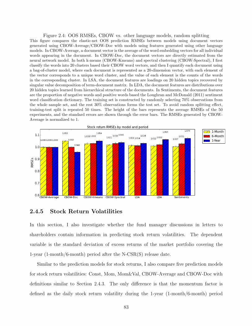
Figure 2.4: OOS RMSEs, CBOW vs. other language models, random splittingThis figure compares the elastic-net OOS prediction RMSEs between models using document vectorsgenerated using CBOW-Average/CBOW-Doc with models using features generated using other languagemodels. In CBOW-Average, a document vector is the average of the word embedding vectors for all individualwords appearing in the document. In CBOW-Doc, the document vectors are directly estimated from theneural network model. In both k-means (CBOW-Kmeans) and spectral clustering (CBOW-Spectral), I firstclassify the words into 20 clusters based their CBOW word vectors, and then I quantify each document usinga bag-of-cluster model, where each document is represented as a 20-dimension vector, with each element ofthe vector corresponds to a unique word cluster, and the value of each element is the counts of the wordsin the corresponding cluster. In LSA, the document features are loadings on 20 hidden topics recovered bysingular value decomposition of term-document matrix. In LDA, the document features are distributions over20 hidden topics learned from hierarchical structure of the documents. In Sentiments, the document featuresare the proportion of negative words and positive words based the Loughran and McDonald (2011) sentimentword classification dictionary. The training set is constructed by randomly selecting 70% observations fromthe whole sample set, and the rest 30% observations forms the test set. To avoid random splitting effect,training-test split is repeated 50 times. The height of the bars represents the average RMSEs of the 50experiments, and the standard errors are shown through the error bars. The RMSEs generated by CBOW-Average is normalized to 1.

2.4.5 Stock Return Volatilities

In this section, I also investigate whether the fund manager discussions in letters to

shareholders contain information in predicting stock return volatilities. The dependent

variable is the standard deviation of excess returns of the market portfolio covering the

1-year (1-month/6-month) period after the N-CSR(S) release date.

Similar to the prediction models for stock returns, I also compare five prediction models

for stock return volatilities: Const, Mom, Mom&Val, CBOW-Average and CBOW-Doc with

definitions similar to Section 2.4.3. The only difference is that the momentum factor is

defined as the daily stock return volatility during the 1-year (1-month/6-month) period

83

ending at the N-CSR(S) release date.

Figure 2.5 shows the OOS prediction RMSEs for stock return volatilities where the

training and test sets are split randomly in the same way as the prediction of stock returns.

We see that vol leadingt has a strong predicting power in predicting future stock return

volatilities, especially for short horizons. However, including the document vectors

generated by CBOW-Average still yields smaller OOS RMSEs. For example, in comparison

to the model Mom, CBOW-Average generates 2.9% less RMSE in predicting 1-month

volatilities, 9.4% less RMSE in predicting 6-month volatilities, and 13.9% less RMSE in

predicting 1-year volatilities. Although CBOW-Doc generates for better results in

predicting long-term volatilities, it underperforms CBOW-Average in prediction short-term

volatilities. These results imply that investment manager discussions contain valuable

information in predicting future stock return volatilities.

2.4.6 Macro Economic Variables

As macro economic conditions is an important factor affecting investment company

performances, and investment manager usually make substantive discussions on ongoing

macroeconomic conditions in their letters to shareholders. I also investigate the predicting

power of the textual features on three important macroeconomic indicators.

The first macroeconomic variable is the annual growth rate of oil prices, which is an

important indicator about the commodity market. I used the West Texas Intermediate

(WTI) oil price data. The second is the growth rate of dollar index, which is an important

indicator about the currency market, I used the Traded Weighted U.S. Dollar Index data.

The third the the growth rate of default spread, which is an important indicator of market

risk. The default spread is defined as the difference between the BAA and AAA corporate

bond rates). All the macroeconomic data are publicly available from the Fred database of

the St. Louis Federal Reserve.

Similar to the prediction models for stock returns, I also compare five prediction models

84

Figure 2.5: Stock return volatility OOS prediction RMSEs with random training-testsplittingThis figure shows the OOS RMSEs in predicting stock return volatilities using five linear models based onelastic-net: (1). “Const”, the explanatory variable include only a constant, which is equivalent to predictionusing historical mean; (2). “Mom”; the explanatory variables include a constant and vol leadingt, thestock return volatilities in the 1-year (1-month/6-month) period prior to the release of N-CSR(S) ; (3).“Mom&Val”, the explanatory variables include a constant, vol leadingt and dividend yieldt; (4). “CBOW-Average”; the explanatory variables include the document vectors generated using the CBOW-Averagemodel in addition to the controlling variables in “Mom&Val”; (5). “CBOW-Doc”, the explanatory variablesinclude the document vectors generated using the CBOW-Doc model in addition to the controlling variablesin “Mom&Val”. The training set is constructed by randomly selecting 70% observations from the wholesample set, and the rest 30% observations forms the test set. To avoid random splitting effect, this procedureis repeated 50 times. The height of the bars represents the average RMSEs of the 50 experiments, and thestandard errors are shown through the error bars. The RMSEs generated by Const is normalized to 1.

for stock return volatilities: Const, Mom, Mom&Val, CBOW-Average and CBOW-Doc with

definitions similar to Section 2.4.3. The only difference is that the momentum factor is

defined as the growth rate of oil price (dollar index/default spread) during the 1-year period

ending at the N-CSR(S) release date.

Figure 2.6 shows the OOS prediction RMSEs for the macroeconomic indicators where

the training and test sets are split randomly in the same way as the prediction of stock

returns. We see that including the document vectors generated by both CBOW-Average

and CBOW-Doc yields significantly smaller OOS RMSEs. For example, in comparison to

the model Const, CBOW-Average generates 13.8% less RMSE in predicting oil price

85

Figure 2.6: Macroeconomic OOS prediction RMSEs with random training-test splittingThis figure shows the OOS RMSEs in predicting macroeconomic indicators using five linear models basedon elastic-net: (1). “Constant”, the explanatory variable include only a constant, which is equivalent toprediction using historical mean; (2). “Mom”; the explanatory variables include a constant and a momentumfactor, where the momentum factor is the grow rate of oil price/dollar index/default spread in the year priorto the release of N-CSR(S) ; (3). “Mom&Val”, the explanatory variables include a constant, the momentumfactor and the value factor dividend yieldt; (4). “CBOW-Average”; the explanatory variables include thedocument vectors generated using the CBOW-Average model in addition to the controlling variables in“Mom&Val”; (5). “CBOW-Doc”, the explanatory variables include the document vectors generated usingthe CBOW-Doc model in addition to the controlling variables in “Mom&Val”. The training set is constructedby randomly selecting 70% observations from the whole sample set, and the rest 30% observations formsthe test set. To avoid random splitting effect, this procedure is repeated 50 times. The height of the barsrepresents the average RMSEs of the 50 experiments, and the standard errors are shown through the errorbars. The RMSEs generated by Const is normalized to 1.

growth rates, 6.8% less RMSE in predicting dollar index growth rates, and 8.2% less RMSE

in predicting default spread growth rates. These results imply that investment manager

discussions contain valuable information in predicting macroeconomic indicators as well.

2.5 Economic Interpretation

In this section, the aim is to understand the economic foundation that explains why

investment manager discussions contain information in predicting stock returns.

Financial economists find that long-term stock returns are predictable. In particular,

numerous studies report that predictive part of the stock returns is risk premium (Pastor and

86

Stambaugh (2009); Cochrane (2008); Campbell and Shiller (1988)). According to standard

asset pricing theory, risk premium is determined by the degree of the risk aversion of a

representative investor. The degree of risk aversion, which reflects the subjective opinions

of an investor, is often difficult to be measured accurately in practice. However, the textual

data of investment manager discussions, which incorporates subjective mental information

of the investors, provide a unique source to measure risk aversion.

I constructed two measures of risk aversion based on the textual data. The first

measure uncertain is the proportion (in percentage) of top 100 words having closest

semantic meaning (highest word vector cosine similarity) to the word “uncertain” (the full

list of words related to the seed words “uncertain”, “risk” and “recession” are shown in

Table 2.8, 2.9 and 2.10 in the Appendix). In theoretical works, economists usually

distinguish uncertainty aversion and risk aversion (Dow and da Costa Werlang (1992)).

Risk describes unknown outcomes whose odds of happening can be measured or learned

about, while uncertainty refers to events that we do not know how to describe. However, in

empirical works, the distinction between risk uncertainty is subtle, and researchers often

ignore it. I adopted the notation of empiricists, where “risk aversion” referred by

empiricists often included both risk aversion and uncertainty aversion, and the empirically

measured risk premium often include a premium for both risk aversion and uncertainty

aversion.

Although I use “uncertain” here as the seeding word, the word list I generate does not

exclusively measure uncertainty aversion only. Checking the full list of words related to

“uncertain”, based on linguistic intuition, it reasonably contains both risk aversion and

uncertainty aversion information. I do not use “risk” as the seeding word because many

words in the list related to “risk” does not have clear risk aversion related interpretation.

The second measure recession is the proportion (in percentage) of top 100 words having

closest semantic meaning to the word “recession”. Previous literature on asset pricing found

that risk aversion correlated with business cycles (Campbell (1999), Boldrin et al. (2001)).

87

In particular, investors usually require a high risk premium. Therefore, when investors start

to talk more about recessions, we can expect the future stock return to be higher.

The OLS regressions results are shown in Table 2.5. We can see that when regressing

return, the annual stock returns post the release date of N-CSR(S) files on uncertain and

recession, both measures of risk aversion predict high returns in the future, which agrees

with our economic intuition that when aversion is high, the expected stock returns is high,

implying high risk premium. In particular, I consider three benchmark models controlling

different variables, the momentum factor return leading and the value factor dividend yield.

Below the coefficients in the Table, I demonstrate the Newey and West (1986) robust

t-test and 5% confidence intervals constructed through bootstrapping of 1,000 times. All

three models generate similar estimates and significant level for uncertain and recession,

indicating that the information contained in these two measures is orthogonal to the

momentum measure return leading and value measure dividend yield.

When we include uncertain and recession separately, both measures are statistically

significant. When uncertain increases by 1 unit, meaning when the proportion of the words

related to “uncertain” increases by 1%, the expected future annual stock returns increases by

5%, which is economically significant. When recession increases by 1 unit, meaning when

the proportion of the words related to “recession” increases by 1%, the expected future

annual stock returns increase by 1%. When we include both uncertain and recession, only

uncertain is significant, which implies the collinearity between uncertain and recession. I

find the correlation between uncertain and recession is 0.257, indicating that uncertain

and recession indeed contains common information.

2.6 Conclusion

In this paper, I construct a unique textual dataset containing 37,014 letters to shareholders

written by investment fund managers to test whether the fund managers discussions

88

Table 2.5: Risk aversion and stock returnsThis table reports the in-sample OLS regression results. The dependent variable return is the annual stockreturns calculated for the 252-day period starting from the day following the release date of N-CSR(S)files. return leading is the annual stock returns calculated for the 252-day period ending at the releasedate of the N-CSR(S) files. dividend yield is the dividend yield, which is log of the dividend to price ratio.uncertain is the proportion of the top 100 words that having the closest semantic relationship with theseeding word “uncertain”, and recession is the proportion of the top 100 words that having the closestsemantic relationship with the seeding words “recession”. The Newey-West Newey and West (1986) HACrobust t-statistics are shown below the estimated coefficient. t-statistics significant at the 1% level are shownin bold.

Const + Risk Aversion Mom + Risk Aversion Mom&Val + Risk Aversion

intercept 0.062 0.077 0.057 0.076 0.090 0.072 0.112 0.094 0.090t-stat 4.590 6.298 4.280 3.751 5.857 3.581 4.466 3.523 3.412

5% CI (0.050, 0.073) (0.063, 0.090) (0.045, 0.070) (0.064, 0.088) (0.072, 0.104) (0.055, 0.088) (0.076, 0.153) (0.058, 0.134) (0.051, 0.132)return leading -0.120 -0.125 -0.120 -0.125 -0.119 -0.120

t-stat -1.371 -1.426 -1.372 -1.420 -1.367 -1.3685% C.I. (-0.176, -0.066) (-0.178, -0.062) (-0.181, -0.068) (-0.178, -0.072) (-0.172, -0.069) (-0.172, -0.063)

dividend yield 0.230 0.190 0.188t-stat 1.381 1.156 1.141

5% C.I. (-0.106, 0.596) (-0.146, 0.558) (-0.143, 0.56)uncertain 0.050 0.048 0.047 0.055 0.047 0.044

t-stat 4.617 4.285 4.354 4.001 4.311 3.9635% C.I. (0.033, 0.068) (0.029, 0.066) (0.032, 0.062) (0.026 0.066) (0.028, 0.065) (0.027, 0.065)

recession 0.011 0.005 0.010 0.005 0.010 0.005t-stat 2.398 1.026 2.347 1.017 2.327 1.009

5% C.I. (0.002, 0.020) (-0.003, 0.013) (0.003, 0.019) (-0.004, 0.015) (0.001, 0.018) (-0.005 0.014)

R2adj 0.012 0.002 0.012 0.027 0.019 0.027 0.027 0.019 0.027

Obs. 2255 2255 2255 2255 2255 2255 2255 2255 2255

contains useful information in predicting stock returns. I quantify the textual documents

using the CBOW neural network work embedding model introduce in Mikolov et al.

(2013a), which represents words and documents in a low-dimensional vector space. My

OOS prediction results using elastic-net show that the fund manager discussions indeed

provide valuable information in predicting stock returns, stock return volatilities, as well as

the growth rates of oil price, dollar index and default spreads. I find that the textual data

reveals information about the degree of risk aversion of institutional investors, which agrees

with previous literature in asset pricing that risk premium is predictable.

89

2.A Appendix

Table 2.6: Text Processing Working SampleThis table demonstrates tokenization of the letters to shareholders extracted from the N-CSRS report filedby Dreyfus GNMA fund on Dec 31, 2014. The original letter extracted from the N-CSRS file through regularexpression matching is much longer, and thus only a paragraph is shown here. Tokens are generated in 5steps: 1. Eliminate HTML markups; 2. Downcase all letters (e.g. convert A-Z to a-z); 3. Separate letterstrings from other types of sequences; 4. Delete strings not a letter, digit, $ or %; 4. Map numerical stringsto #; 5. Clean up whitespace, leaving only one white space between tokens. The McDonald financial Englishword dictionary is used to filter out tokens that are not an English word; 6. Eliminate stopwords.

Original letter Contrary to most analysts’ expectations, U.S. fixed-incomesecurities generally gained value as long-term interest rates fellover the reporting period. Under most circumstances, bond yieldstend to climb and prices fall during economic recoveries such asthe one that prevailed over the past six months. However,international developments led to a surge in demand for arelatively limited supply of U.S. government securities, causing asupply-and-demand imbalance that drove yields lower and priceshigher. Higher yielding sectors of the bond market also faredrelatively well as credit conditions improved in the recovering U.S.economy. We currently hold a relatively cautious view of the near-to intermediate-term prospects for fixed-income securities.

Tokenized letter contrary most analysts expectations fixed income securitiesgenerally gained value long term interest rates fell over reportingperiod under most circumstances bond yields tend climb pricesfall during economic recoveries such one prevailed over past sixmonths however international developments led surge demandrelatively limited supply government securities causing supplydemand imbalance drove yields lower prices higher higher yieldingsectors bond market also fared relatively well credit conditionsimproved recovering economy currently hold relatively cautiousview near intermediate term prospects fixed income securities

90

Table 2.7: Letter length summary statisticsThis table shows the summary statistics of the length (number of words) of the tokenized letters in eachyear. Count is the number of letters extracted from N-CSR(S) files in each year. Mean is the average numberof words in the letters. Std is the standard deviation of the letter lengths. X% are the X percentile of theletter lengths.

Year Count Mean Std 5% 50% 95%

2003 1987 407 548 67 255 11692004 3624 413 554 99 262 10912005 3569 451 591 98 294 12652006 3350 428 570 85 258 12132007 3215 463 608 99 274 13802008 3259 523 640 67 340 16332009 3283 515 601 75 312 15562010 2979 472 576 78 267 15112011 3045 487 597 73 285 15552012 2887 482 560 60 295 15162013 2890 515 843 60 305 16252014 2926 496 585 57 305 1622

91

Table 2.8: Risk aversion wordsThis table demonstrates words related to risk aversion. The three word lists are generated by three seedingwords: “recession”, “risk” and “uncertain”. Each list contains 100 words with highest semantic similaritywith the seeding words, where the semantic similarity of a pair of words is measured as the cosine similarityof their word embedding vectors.

recession risk uncertain

Related Word Similarity Related Word Similarity Related Word Similarity

1 depression 0.556 risks 0.481 unsettled 0.5072 slump 0.499 risky 0.426 challenging 0.5043 contraction 0.495 riskier 0.398 turbulent 0.4874 recessions 0.483 volatility 0.374 unstable 0.4515 downturn 0.478 quality 0.371 skeptical 0.4456 slowdown 0.451 beta 0.320 unclear 0.4457 crisis 0.440 swaps 0.314 uncertainty 0.4408 deflation 0.439 coupons 0.309 tough 0.4359 officially 0.409 sensitivity 0.306 cloudy 0.43410 crunch 0.396 yielding 0.305 constructive 0.42311 recessionary 0.396 potential 0.295 uncertainties 0.42112 correction 0.390 exposure 0.295 evolving 0.41313 patch 0.381 seasonally 0.286 vigilant 0.41114 economists 0.374 potentially 0.283 accommodating 0.40915 contagion 0.372 float 0.279 fragile 0.40616 wwii 0.370 flexibility 0.272 changing 0.40317 recovery 0.370 attractiveness 0.272 cautious 0.39718 winter 0.368 safety 0.268 flux 0.39419 mess 0.367 probability 0.267 sanguine 0.39320 collapse 0.364 defensive 0.262 tenuous 0.38221 meltdown 0.361 traditional 0.259 murky 0.38122 sars 0.361 thereby 0.259 choppy 0.37923 epidemic 0.360 correlation 0.259 dangerous 0.37424 catastrophe 0.352 compensate 0.255 stormy 0.37225 shock 0.352 conviction 0.255 perplexing 0.37126 war 0.352 likelihood 0.255 mindful 0.37027 storm 0.352 option 0.248 optimistic 0.36828 technically 0.352 rated 0.247 clouded 0.36629 landing 0.349 exposures 0.245 adapting 0.36430 deflationary 0.349 fluctuation 0.245 confusing 0.36231 economy 0.347 actively 0.243 tense 0.35932 breakup 0.346 willing 0.242 volatile 0.35333 malaise 0.346 environment 0.242 unsettling 0.352

92

Table 2.9: Risk aversion words (continue)This table demonstrates words related to risk aversion. The three word lists are generated by three seedingwords: “recession”, “risk” and “uncertain”. Each list contains 100 words with highest semantic similaritywith the seeding words, where the semantic similarity of a pair of words is measured as the cosine similarityof their word embedding vectors.

recession risk uncertain

Related Word Similarity Related Word Similarity Related Word Similarity

34 slow 0.344 spreads 0.242 interdependent 0.35035 subside 0.340 conservative 0.239 react 0.35036 calamity 0.340 avoiding 0.239 navigating 0.35037 scenario 0.340 incremental 0.238 bearish 0.34838 syndrome 0.338 inefficiencies 0.237 conducive 0.34839 stall 0.337 correlated 0.237 difficult 0.34840 soft 0.337 safer 0.237 elusive 0.34541 dip 0.337 liquid 0.236 nimble 0.34142 damage 0.335 unavoidable 0.236 reality 0.34043 acceleration 0.335 degree 0.236 tougher 0.33744 deteriorate 0.333 diversification 0.235 bleak 0.33645 layoffs 0.331 safe 0.235 unpredictability 0.33646 faltering 0.330 speculative 0.233 comfortable 0.33647 gdp 0.327 spread 0.233 steadfast 0.33448 appears 0.326 possibility 0.232 precarious 0.33449 protracted 0.325 tactically 0.232 upbeat 0.33250 cold 0.324 fluctuations 0.232 pessimistic 0.33251 expansion 0.323 cds 0.232 unknown 0.33252 lengthiest 0.323 approach 0.230 transitional 0.33153 britain 0.321 commensurate 0.228 nervous 0.32454 summer 0.319 prudent 0.228 complicated 0.32455 disruption 0.319 hedges 0.228 unpredictable 0.32056 bubble 0.318 uncorrelated 0.227 unresolved 0.31957 crises 0.318 emphasis 0.226 challenge 0.31858 slide 0.317 dispersion 0.226 erratic 0.31359 fragility 0.317 concentrate 0.225 confident 0.31260 rough 0.313 yield 0.225 brighter 0.31161 verge 0.313 upside 0.224 uncomfortable 0.31162 sliding 0.313 transparency 0.223 frustrating 0.31163 bounce 0.312 seek 0.223 daunting 0.30964 deceleration 0.311 distressed 0.221 bullish 0.30865 deleveraging 0.310 alternatives 0.221 preparing 0.30766 boom 0.309 caution 0.221 wary 0.307

93

Table 2.10: Risk aversion words (continue)This table demonstrates words related to risk aversion. The three word lists are generated by three seedingwords: “recession”, “risk” and “uncertain”. Each list contains 100 words with highest semantic similaritywith the seeding words, where the semantic similarity of a pair of words is measured as the cosine similarityof their word embedding vectors.

recession risk uncertain

Related Word Similarity Related Word Similarity Related Word Similarity

67 nber 0.309 diversifying 0.221 buoyant 0.30768 fragile 0.308 sensitive 0.220 tricky 0.30769 surface 0.307 stability 0.219 unknowns 0.30770 seems 0.306 movements 0.218 dire 0.30671 implosion 0.304 seeking 0.218 fluid 0.30672 hurricanes 0.303 strategies 0.217 clearer 0.30473 appeared 0.302 reallocate 0.216 serious 0.30374 commentators 0.302 insatiable 0.216 intact 0.30375 problem 0.301 valuations 0.216 inopportune 0.30376 jeopardy 0.300 devalued 0.216 valid 0.30277 expecting 0.299 cashflow 0.214 ideal 0.30278 goldilocks 0.299 hungry 0.214 cognizant 0.30179 weaken 0.298 protection 0.214 interconnected 0.29880 recoveries 0.298 safest 0.213 benign 0.29881 recede 0.298 duration 0.213 question 0.29482 cooling 0.297 directional 0.212 challenged 0.29383 strains 0.297 patient 0.210 recessionary 0.29284 clouds 0.297 prone 0.210 proactive 0.29185 attack 0.297 liquidity 0.209 muted 0.29086 katrina 0.295 advantage 0.208 inevitable 0.29087 yet 0.295 systematically 0.208 shifting 0.28988 decelerate 0.295 demanded 0.207 skittish 0.28789 unemployment 0.295 selectively 0.206 certainty 0.28790 bottoming 0.294 instruments 0.206 grapple 0.28791 spiral 0.294 asymmetric 0.205 troubling 0.28792 doldrums 0.294 desire 0.205 rewarding 0.28793 slowing 0.294 structured 0.205 critical 0.28694 crash 0.293 capture 0.204 today 0.28495 problems 0.293 sought 0.204 frustrated 0.28496 trouble 0.292 favoring 0.204 conscious 0.28497 stagnation 0.291 riskiest 0.202 elevated 0.28398 slowly 0.291 cues 0.202 subdued 0.28299 lasting 0.290 correlations 0.201 exacting 0.282100 danger 0.290 environments 0.201 tumultuous 0.281

94

Table 2.11: LSA Sample TopicsThis table demonstrates sample words and their corresponding loadings of three latent topics generated byLSA.

Topic 1 Topic 2 Topic 3

Word Loading Word Loading Word Loading

1 municipal 0.086 vanguard 0.512 pioneer 0.1522 vanguard 0.075 admiral 0.181 federated -0.0793 bonds 0.070 municipal -0.131 retirement 0.0724 fed 0.065 prudential 0.106 strategists -0.0705 index 0.061 mason -0.096 register -0.0676 bond 0.059 revenue -0.078 shareowners 0.0527 tax 0.057 state -0.078 tips 0.0518 yield 0.057 star 0.073 allocations 0.0489 cap 0.054 wellington 0.072 fed 0.047

10 shares 0.054 shares 0.071 odyssey -0.04711 yields 0.053 hospital -0.070 planning -0.04612 securities 0.052 rated -0.069 listing -0.04413 crisis 0.052 municipals -0.068 disclaim 0.04414 credit 0.052 pioneer 0.067 crisis -0.04315 treasury 0.051 peer 0.066 capabilities -0.04116 global 0.051 expense 0.064 prudential -0.04117 exempt 0.051 free -0.063 shareowner 0.04118 sector 0.051 curve -0.061 timers 0.04019 funds 0.050 tobacco -0.060 municipal -0.03820 debt 0.050 odyssey 0.057 tapering 0.03721 stocks 0.049 credit -0.056 tools -0.03722 rate 0.049 bonds -0.055 insights -0.03523 class 0.048 efficient -0.054 actual 0.03424 company 0.048 fed -0.053 updates -0.03425 emerging 0.047 issuance -0.052 glossary 0.03426 six 0.047 ratios 0.052 vanguard -0.03427 quarter 0.046 explorer 0.052 covering -0.03328 recovery 0.046 obligation -0.052 easy -0.03329 companies 0.045 advisors 0.051 allocation 0.03230 trust 0.045 caps 0.051 mason 0.032

95

Table 2.12: LDA Sample TopicsThis table demonstrates sample words and their corresponding loadings of three latent topics generated byLDA.

Topic 1 Topic 2 Topic 3

Word Loading Word Loading Word Loading

1 toreador 0.080 misinterpreted 0.141 barrow 0.0472 agonizingly 0.041 moat 0.116 upright 0.0393 accesses 0.039 tapering 0.099 overextended 0.0234 unacceptably 0.037 masters 0.097 motion 0.0205 shippers 0.026 dispersion 0.080 oddest 0.0156 spree 0.026 quo 0.070 digests 0.0157 homepage 0.021 palm 0.065 persuading 0.0158 saddened 0.019 emissions 0.062 reissuance 0.0149 intending 0.019 scares 0.056 affixed 0.014

10 traverse 0.019 succeeding 0.054 perpetuating 0.01211 abstained 0.017 hepatitis 0.054 genius 0.01112 squabbles 0.017 embarks 0.053 stymie 0.01113 unjustifiably 0.017 disputed 0.052 upticks 0.00914 axiom 0.016 micron 0.051 summarily 0.00915 animated 0.016 circle 0.051 technicians 0.00916 tornado 0.015 fracking 0.051 surpasses 0.00817 chipset 0.015 scare 0.050 messy 0.00818 died 0.014 wintergreen 0.050 glory 0.00719 refurbished 0.014 nimble 0.048 soil 0.00720 derailment 0.013 mega 0.047 doubting 0.00721 swank 0.013 excelsior 0.047 conserve 0.00622 opponent 0.013 scene 0.047 wield 0.00623 bender 0.013 dodge 0.047 backs 0.00624 honey 0.012 luck 0.045 nimble 0.00625 nondeductible 0.012 dependence 0.044 exhorting 0.00626 irrationally 0.012 crossover 0.044 transnational 0.00527 birds 0.012 intrepid 0.044 woke 0.00528 revoked 0.011 obscured 0.044 conformed 0.00529 representational 0.011 environmentally 0.042 impetuous 0.00530 doctrine 0.011 perpetual 0.042 backstops 0.005

96

Figure 2.7: Sentiment words visualization based on t-SNEThis figure demonstrates the clusters of sentiment words. The original word vectors learned in the CBOWmodel have 300 dimension, and they are projected onto a 2-dimension vector space using t-SNE. Thehorizontal and vertical axis represents the first and second dimension of the t-SNE dimension reduced spacerespectively. The green dots are positive words, and red dots are negative words. Positive words are top 40words with highest cosine similarity to “good” , and the negative words are top 40 words with highest cosinesimilarity to “bad”.

97

Fig

ure

2.8:

Sen

tim

ent

wor

ds

vis

ual

izat

ion

bas

edon

t-SN

ET

his

figu

redem

onst

rate

sth

ecl

ust

ers

ofth

ew

ord

sre

late

dto

diff

eren

tec

on

om

icto

pic

s.T

he

ori

gin

al

word

vect

ors

learn

edin

the

CB

OW

mod

elh

ave

300

dim

ensi

ons,

and

they

are

pro

ject

edon

toa

2-d

imen

sion

vect

or

space

usi

ng

t-S

NE

.T

he

hori

zonta

lan

dver

tica

laxis

rep

rese

nts

the

firs

tan

dse

con

dd

imen

sion

ofth

et-

SN

Ed

imen

sion

red

uce

dsp

ace

resp

ecti

vel

y.E

ight

econ

om

icto

pic

sare

show

nin

the

gra

ph

:re

gio

ns,

poli

tics

,m

acr

oec

on

om

y,m

arke

tin

dex

,co

mm

od

ity,

ind

ust

ry,

inve

stm

ent

an

dsh

are

hold

er.

To

gen

erate

the

word

list

for

each

top

ic,

Iu

seth

ekey

word

s“re

gio

n”,

“p

oli

tics

”,

“mac

roec

onom

y”,

“in

dex

”,“c

omm

od

ity”,

“in

du

stry

”,

“in

vest

men

t”,

“sh

are

hold

er”

as

seed

word

s,an

dfi

nd

30

word

sth

at

hav

eth

eh

ighes

tse

manti

csi

mil

arit

yto

the

seed

wor

dfo

rea

chto

pic

.

98

Chapter 3

Corporate Takeovers and Cash

Holdings

Abstract

This paper investigates the relationship between the motivation of making acquisitions and

precautionary cash holding behaviors of a firm. I develop a dynamic choice model with

heterogeneous agents. The model is discrete in time and has an infinite horizon. Cash

provides cheap financing source for making acquisitions in both current and future periods.

The effect of reducing future acquisition cost originates from the model dynamics that firms

have the option to make repeated acquisitions, which is not possible in a static model. I

solve the model numerically and calibrate it to the U.S. market data. I find that when the

opportunities of making acquisitions increase, market wide cash reserve increases, as firms

accumulate cash to make acquisitions or to attract acquirers.

Key Words: mergers, acquisitions, cash holding, entry, exit, dynamic

JEL Classification: C61, C63, C68, C78, G32, G34, G35,

99

3.1 Introduction

One of the most important motivations for firms to hold cash is to transfer liquidity across

time to buffer negative shocks to cash flows in the future, so as to avoid missing investment

opportunities due to liquidity shortage. Making acquisitions is an important type of

investment, and the precautionary motivation of holding cash to facilitate acquisitions can

be economically significant. In this paper, I develop a dynamic choice model to study the

relationship between the motivation of making acquisitions and cash holding behaviors of a

firm.

I find that an increase in acquisition opportunities induces firms to hold more cash on

average. This phenomenon can be explained by that both acquirers and targets hold more

cash than stand-alone firms, so an increase in acquisition opportunities leads to a lower

proportion of stand-alones in the economy and thus the economy-wide average cash

holdings increase. Acquirers tend to hold more cash than stand-alones because of their

larger motivations to avoid external financing cost. Targets tend to hold more cash than

stand-alones to attract acquirers since acquirers can use the cash of the target to reduce

external financing cost. I also find that getting acquired is an important alternative to exit

the market. Getting acquired is attractive because target firms can share part of the

merger synergy benefit as acquisition premium in addition to firm value. Finally, I find

that acquisitions generally happen between high-value acquirers and low-value targets.

The model is discrete in time and has an infinite horizon. At the beginning of each period,

a firm in the market observes its productivity, which is determined by an exogenous AR(1)

process. Then the firm is matched with a partner with a constant probability. If the firm

acquires its partner, it makes a payment to the shareholders of the target firm, where the

payment is equal to the value of the target firm plus a premium determined by the synergy

benefit of the merger as well as the Nash bargaining power of the two parties. The acquirer

has the option of financing its acquisition payment using internal funds or raising external

funds with additional cost. Reasons for external financing to be costly include adverse

100

selection premium, flotation costs, tax costs and so on (Fazzari et al. (1988)). Available

internal funds are limited by the sum accumulated cash reserves and cash flow generated in

the concurrent period. If internal funds are insufficient, the acquirer has to finance the gap

by raising external funds.

Entry and exit is also incorporated in the model. At the beginning of each period,

potential entrants can enter the market by paying a one-time entry cost. At the end of

each period, incumbents can choose to exit the market if the exit value is larger than their

continuation value. The option of entry and exit is an important ingredient to generate a

stationary equilibrium, as the size of the market will shrink continuously without entry of

new firms due to acquisitions.

I solve the model numerically and calibrate the parameters to match seven empirical

moments. I use the merged data set of SDC Platinum M&A (mergers and acquisitions)

and Compustat. The SDC Platinum M&A data set contains corporate takeover information

for the U.S. market since 1971 and Compustat contains corporate fundamentals. It turns

out the simulated moments generated by my calibrated model can match their empirical

counterparts well.

This paper firstly contributes to the literature that studies precautionary cash holdings.

Using publicly traded U.S. firms data in the 1971-1994 period, Opler et al. (1997) find

evidence supporting that firms with stronger growth opportunities and riskier cash flows

hold a larger proportion of cash. Han and Qiu (2007) find that cash holdings of financially

constrained firms are sensitive to cash flow volatility using a sample of publicly traded

companies in the U.S. from 1997 to 2002. Acharya et al. (2007) model the interplay between

cash and debt policies and show that cash allows firms facing financial constraint to hedge

against income shortfalls. Morellec and Nikolov (2009) study a real options model and find

that cash holdings are used to cover unexpected operating losses and to avoid inefficient

closure. Nikolov et al. (2013) find cash to be an important instrument to absorb shocks and

fund investment opportunities for small and financially constrained firms.

101

In particular, several empirical works have shown the importance of cash holdings on

firms’ M&A decisions. Harford (1999) finds that firms with more cash holdings are more likely

to make acquisitions and this can be explained by agency costs of free cash holding. This

paper is a supplement to the precautionary cash holding theory as my model implies that a

firm’s cash holding policy is affected not only by its cash flow uncertainty, but also by the cash

flow volatilities of other firms, as well as other factors that influence its expected acquisition

payoffs. Pinkowitz et al. (2002) find that the likelihood for a firm to be a target is negatively

related to the excess cash holding of the firm as managers hold cash to entrench themselves

at the expense of shareholders. Although the finding is different from the implication of my

model in this paper, it does not directly contradicts the model because the model focuses the

functionality of cash as cheap financing source and does not incorporate the agency problem.

Several theoretical works have investigated the dynamics of M&A and its effects on an

industry equilibrium. Morellec and Zhdanov (2005) build a dynamic model incorporating

competition and imperfect information to determine the terms and timing of takeovers.

David (2011) sets up a search and matching model to learn the impacts of M&A on aggregate

economic performance. Dimopoulos and Sacchetto (2012) develop a model of a competitive

industry with heterogeneous firms to study the industry dynamics of investments, M&A and

entry and exit. The main contribution of this paper is building a bridge between corporate

financing behaviors and the dynamics of M&A and entry and exit.

The remaining part of this paper is organized as follows. Section 2 develops a dynamic

model with cash holdings, acquisitions, as well as entry and exit. Section 3 solves the model

numerically and calibrate it. Section 4 presents the comparative static analysis and discuss

the implications of the model. Section 5 concludes.

102

3.2 Model

The model I present in this section is derived from the one in Dimopoulos and Sacchetto

(2012). I model an industry in which firms have dynamic choices of cash holdings,

acquisitions, as well as entry and exit. The model is discrete in time with an infinite

horizon. In each period, denote the number of incumbents firms as N and the number of

potential entrants as NE.

The timing of actions is shown in Figure 3.1. At the beginning of a period, an incumbent

firm first observes the shock to its productivity and then it will be matched with a partner

with an exogenously determined probability. The firm matched with a partner makes the

decision of acquisition based on the comparison between the value of acquisition and value

of standing alone. After the choice of acquisition or standing alone, an incumbent chooses

its cash holdings for the next period and then the current period payoff will be realized. At

the end of the period, an incumbent makes the choice of exit. If it exits, its cash holdings

are paid to shareholders; otherwise, it holds cash to next period.

At the beginning of each period, a potential entrant firstly observes a signal about its

productivity. If it enters the market, it pays a fixed one-time entry cost and becomes an

entrant. I assume that an entrant does not hold cash, and it is involved in matching and

acquisition and does not exit in the period of entry. It generates cash flows based on its

productivity and it chooses its cash holding.

Production and profits The production function for each firm is π − qF , in which π ∈

[π, π] is a productivity, which follows a log AR(1) process ln π′ = ρ lnπ + ε, where ρ ∈ (0, 1)

and ε ∼ N (0, σπ) i.i.d.. qF is a fixed cost of production. Denote the transition function of π

as FΠ (π′|π).

Acquirer or target In each period, an incumbent firm is matched with a partner with

a constant probability µ. Among a pair of matched firms, each firm is willing to make an

103

Figure 3.1: Timing of actions

acquisition if its acquisition value is larger than their stand-alone value. If there is only one

firm that is willing to make the acquisition, it becomes the acquirer. If both firms are willing

to make the acquisition, I assume that the firm that benefits more from acquisition1 becomes

the acquirer. The acquirer makes a payment to the target shareholders in the acquisition.

The payment is equal to the value of the target firm plus a premium. The premium is

determined by the Nash bargaining power of the two counter-parties in the acquisition deal.

The process of Nash bargaining is not modeled explicitly and the premium is assumed to be

proportional to the target value. The proportion coefficient is γ.

In the period of acquisition, the cash holding of an acquirer is cA = c + cT , where c

is cash holding of the acquirer before acquisition and cT is the cash holding of its target.

The productivity of the acquirer in the period of acquisition is given by synergy function2

(Dimopoulos and Sacchetto (2012)):

πA (π, πT ) = π + π − π [λmax {π, πT}+ (1− λ) min {π, πT}] θ, (3.1)

1This is determined in the following way: Suppose Firm A and Firm B are matched. I first calculate thestand-alone value for either firm. Then, assuming Firm A as acquirer and Firm B as target, I can calculatethe acquisition value for Firm A; similarly, assume Firm A as target and Firm B as acquirer I can calculatethe acquisition value of Firm B. If acquisition value of Firm A - stand-alone value of Firm A ¿ acquisitionvalue of Firm B - stand-alone value of Firm B, Firm A will be the potential acquirer and Firm B will be thepotential target. Otherwise, Firm A will be the potential target and Firm B will be the potential acquirer.The idea of this assumption is straight forward: if the two firms compete to be the acquirer in an auction,the one with high larger difference between its acquisition value and stand-alone value is willing to pay more.

2An example plot using my calibrated parameter values for this function is shown in Figure 3.2

104

where π is the productivity of the acquirer before acquisition and πT is the productivity of

the target, and π = π−ππ−π , λ ≥ 0 and θ ∈ (0, 1). πA is scaled in such a way that it never lies

out of the interval [π, π]. When λ is large, the largest improvements in productivity occurs

when firms with very different productivity merge; when λ is small, the largest improvements

in productivity occurs when firms with similar productivity merge. θ captures the curvature

of the synergy function. The next period productivity of the acquirer is determined by

transition FΠ (π′|πA).

Cash holdings Assuming the interest income of cash holding can be ignored, it is costly

for firms to hold cash. The benefit of holding cash is to avoid costly external financing when

making acquisitions. Balancing the cost and benefit of cash determines the optimal cash

holding level.

At the beginning of each period, an incumbent firm holds cash c. The sum of cash holding

and profits generated in the current period is total internal funds available for financing

acquisitions. After acquisition, acquirers and stand-alone firms choose cash holding c′ for

the next period. Whenever internal funds are insufficient, an acquirer can raise external

funds to finance its acquisition payments, incurring additional financing cost. I assume the

external financing cost to be proportional (with coefficient φ) to the amount of fund raised.

At the end of a period, cash in addition to c′ is paid to shareholders as dividends.

In reality, acquisitions payments include all-stock payment, mixed of securities and cash,

an all-cash payment. For simplicity, I only consider all-cash payments in my model.

Entry and exit At the beginning of each period, there is a pool of NE potential entrants.

A potential entrant observes a signal πE regarding their profitability drawn from a time-

invariant distribution G (πE), and then decides whether to pay an entry cost qE and enter

the market. An entrant is immediately productive but it does not hold cash when entering

the market. In addition, it is not involved in acquisitions and cannot exit in the period of

entry.

105

At the end of each period, existing incumbents (acquirers and stand-alones) makes the

choice between exit and stay. The payoff of an exiting firm is equal to it liquidation value. As

the dynamics of corporate assets other than cash is not explicitly modeled. The liquidation

of value is equal to the value of cash.

Value function Based on the model set-up, the value of a stand-alone incumbent is

V (π, c) = max

{maxc′

{d (1 + φ1 (d < 0)) +

1

1 + rV C (π, c′)

}, d+ c′

}(3.2)

where V C (π, c′) is the expected end-of-period continuation value, which incorporates the

value of the option of becoming an acquirer or a target in the future. d = c + π − qF − c′

denotes current period cash flow and negative cash flow implies raising external funds. A

firm exits whenever the value of stay is smaller than the exiting value:

maxc′{d (1 + φ1 (d < 0)) + 1

1+rV C (π, c′)

}< d+ c′.

The value of an acquirer is

VA (π, c, πT , cT ) = max

{maxc′A

{dA (1 + φ1 (dA < 0)) +

1

1 + rV C (πA, c

′A)

}, dA + c′A

}(3.3)

where dA = cA + πA − qF − V (πT , cT ) − γW (π, c, πT , cT ) − c′A − qI denotes the cash flow

of the acquirer, which is equal to the sum of cash holdings of the two matched firms (cA =

c + cT ), plus the production πA of the acquirer, and net off payments (qF + V (πT , cT ) +

γW (π, c, πT , cT )) to the shareholders of the target, cash holding for next period c′A and

integration cost qI .

The acquisition synergy benefit of an acquisition is defined as the difference between the

acquirer’s value and its otherwise stand-alone value:

W (π, c, πT , cT ) = VA (π, c, πT , cT )− V (π, c) . (3.4)

An potential acquirer will make acquisition if W (π, c, πT , cT ) ≥ 0.

106

Since an incumbent will be matched with a partner with probability µ, the continuation

value for Firm i with matching partner Firm j is

V C (πi, c′) =´Cj

´Πj

´Πi

[V (π′i, c′) + µmax {1 (W (π′i, c

′, πj, cj) > W (πj, cj, π′i, c′))W (π′i, c

′, πj, cj)

+1 (W (π′i, c′, πj, cj) < W (πj, cj, π

′i, c′)) γW (πj, cj, π

′i, c′) , 0}] f (πj, cj) dFΠ (π′i|πi) dπjdcj

(3.5)

where f (πj, cj) denotes the stable joint density function of production and cash holding of

firms in the economy. The integrand contains two parts. V (π′i, c′) is the stand-alone value for

Firm i in next period. The product of µ and the max term is the value of acquisition. When

W (π′i, c′, πj, cj) > W (πj, cj, π

′i, c′), it means the acquisition benefit for Firm i is larger than

the acquisition benefit of Firm j, and thus Firm i becomes the acquirer and the acquisition

value is W (π′i, c′, πj, cj). When W (π′i, c

′, πj, cj) < W (πj, cj, π′i, c′), the acquisition benefit

for Firm j is larger and Firm j becomes the target, and the value of getting acquired is

γW (πj, cj, π′i, c′). The case that W (π′i, c

′, πj, cj) = W (πj, cj, π′i, c′) is not included in the

expression because it has zero measure.

The value function for a potential entrant is

VE (πE) = max

{maxc′E

{dE (1 + φ1 (dE < 0)) +

1

1 + rV C (πE, c

′E)

}, 0

}, (3.6)

where dE = πE − qF − qE − c′E is the cash flow for an entrant and c′E is the cash held for

the next period of the entrant. A potential entrant enters if

maxc′E{dE (1 + φ1 (dE < 0)) + 1

1+rV C (πE, c

′E)}≥ 0.

Equilibrium E ={πE ∈ Π : maxc′E

{dE (1 + φ1 (dE < 0)) + 1

1+rV C(πE, c

′E)}≥ 0}

denotes the set of the new entrant’s production signals, which contains signals large enough

that makes it profitable for a potential entrant to enter the market, and

PE = Prob [πE ∈ E ] denotes the entering probability.

S ={

(π, c) ∈ Π× C : maxc′{d (1 + φ1 (d < 0)) + 1

1+rV C (π, c′)

}≥ d+ c′

}is the set of

production shocks and cash holdings for an incumbent firm that is not matched with a

107

partner to not exit, and PS = Prob [(π, c) ∈ S] denotes the probability.

A (πT , cT ) =

{(π, c) ∈ Π× C : max

c′A

{dA (1 + φ1 (dA < 0)) +

1

1 + rV C

(πA, c

′A

)}≥ d+ c′A,W (π, c, πT , cT ) ≥ max [0,W (πT , cT , π, c)]

}

is the set of productions and cash holdings of firms that acquire a target with production

πT and cash holding cT and do not exit.

N (πT , cT ) =

{(π, c) ∈ Π× C : max

c′

{dA (1 + φ1 (dA < 0)) +

1

1 + rV C

(πA, c

′)} ≥ d+ c′,max [W (π, c, πT , cT ) ,W (πT , cT , π, c)] < 0

}

is the set of shocks of firms that stand alone and do not exit, even though they are matched

with a partner with production πT and cash holding cT .

The equilibrium is a collection of value functions V (π, c), VA (π, c, πT , cT ), VE (πE); cash

holding functions c′ (π, c), c′A (π, c, πT , cT ), c′E (πE); cross-sectional densities of incumbent’s

profitability ft (Π, C), and the incumbents measure Nt, such that

1. A stand-alone firm with production π and cash holding c chooses c′ (π) to maximizes

it value V (π, c);

2. An acquirer with production π and cash holding c, when matched with a target with

production πT and cash holding cT , chooses c′A (π, c, πT , cT ) to maximize its value

VA (π, c, πT , cT );

3. An entrant with production πE chooses c′ (πE) to maximize its value VE (πE);

4. Firms within a matching pair optimally make the choice of acquisitions;

5. For all Borel sets (Π, C) ∈∏×C and for all t ≥ 0

ft+1 (Π, C) = ft+1

(Π, C

∣∣∣Et = 1)P (Et = 1) + ft+1

(Π, C

∣∣∣Et = 0)P (Et = 0) . (3.7)

where P (Et = 1) = NEt/ (NEt +NSt) is the probability for an incumbent firm in period

t+1 to be an entrant in period t, where NEt = NEPE is the number of entrants in period

t and NSt = Nt [(1− µ)PS + µ (PA/2 + PN)] is the number of incumbents that do not

108

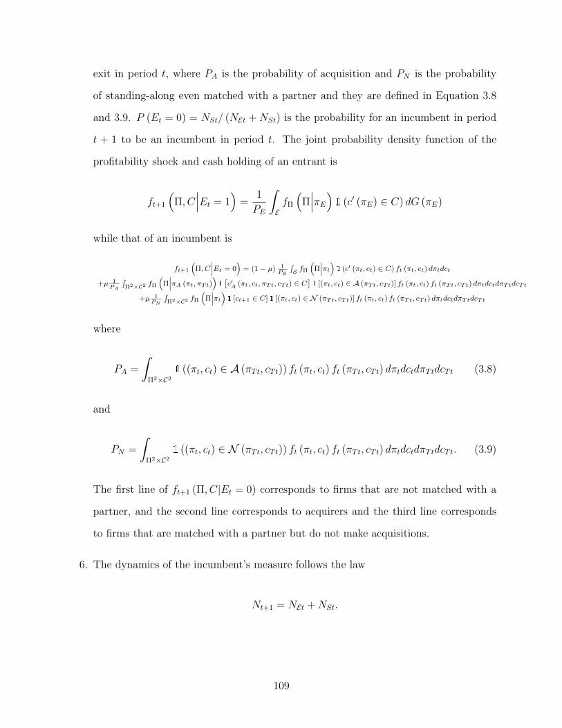
exit in period t, where PA is the probability of acquisition and PN is the probability

of standing-along even matched with a partner and they are defined in Equation 3.8

and 3.9. P (Et = 0) = NSt/ (NEt +NSt) is the probability for an incumbent in period

t + 1 to be an incumbent in period t. The joint probability density function of the

profitability shock and cash holding of an entrant is

ft+1

(Π, C

∣∣∣Et = 1)

=1

PE

ˆEfΠ

(Π∣∣∣πE)1 (c′ (πE) ∈ C) dG (πE)

while that of an incumbent is

ft+1

(Π, C

∣∣∣Et = 0)

= (1− µ) 1PS

´S fΠ

(Π∣∣∣πt)1 (c′ (πt, ct) ∈ C) ft (πt, ct) dπtdct

+µ 1PA

´Π2×C2 fΠ

(Π∣∣∣πA (πt, πTt)

)1[c′A (πt, ct, πTt, cTt) ∈ C

]1 [(πt, ct) ∈ A (πTt, cTt)] ft (πt, ct) ft (πTt, cTt) dπtdctdπTtdcTt

+µ 1PN

´Π2×C2 fΠ

(Π∣∣∣πt)1 [ct+1 ∈ C]1 [(πt, ct) ∈ N (πTt, cTt)] ft (πt, ct) ft (πTt, cTt) dπtdctdπTtdcTt

where

PA =

ˆΠ2×C2

1 ((πt, ct) ∈ A (πTt, cTt)) ft (πt, ct) ft (πTt, cTt) dπtdctdπTtdcTt (3.8)

and

PN =

ˆΠ2×C2

1 ((πt, ct) ∈ N (πTt, cTt)) ft (πt, ct) ft (πTt, cTt) dπtdctdπTtdcTt. (3.9)

The first line of ft+1 (Π, C|Et = 0) corresponds to firms that are not matched with a

partner, and the second line corresponds to acquirers and the third line corresponds

to firms that are matched with a partner but do not make acquisitions.

6. The dynamics of the incumbent’s measure follows the law

Nt+1 = NEt +NSt.

109

3.3 Calibration

To investigate the dynamics of cash holdings, acquisitions, entries and exits of firms in the

economy, I solve the model numerically using a technique combining value function

iteration and density function iteration, and calibrate the parameters to match seven

empirical moments. The algorithm for solving the equilibrium numerically is described in

the Appendix. In this section, I introduce the dataset and discuss the empirical moments

used in the calibration.

3.3.1 Data

The corporate takeover transactions data are from the Thomson Reuter’s SDC Platinum

database. I apply filters similar to those in Dimopoulos and Sacchetto (2012) to construct

my sample. The M&A dataset includes completed transactions categorized as mergers or

acquisitions of majority interest. The transactions cover the period of 1981-2010 in the U.S.

market. I exclude deals in which: the bidder holds more than 50% of the target’s shares at

the announcement date of bid; the bidder is seeking to acquire less than 50% of the target

shares; there is no information on the percentage of shares involved in the transaction; the

acquirer or target is a regulated utility (SIC codes 4900 to 4949), a financial institution (SIC

codes 6000 to 6799), or a quasi-public firm (SIC codes greater than 9000); the identity of

the acquirer is not disclosed or attributable to a specific entity (e.g. “investor group”).

The corporate fundamentals data are from Compustat. The variables are summarized in

Table 3.1. I merge the observations in SDC Platinum with the Compustat database using

CUSIP.

3.3.2 Parametrization and calibration targets

As mentioned in Dimopoulos and Sacchetto (2012), the measure of potential entrants NE

affects the size of the simulated economy but does not affect the simulated moments in steady

110

state, and I set N = 1000 and NE = 200 in the calibration.

One period in the simulation is assumed to correspond to one year. Panel A of Table

3.3 displays parameters with values taken from previous works that share similar modeling

specifications. r is set to be 0.04, which is commonly used in the corporate finance literature.

Following Dimopoulos and Sacchetto (2012), I set the probability of matching µ to be 0.34,

merger synergy weight λ to be 0.55 and merger synergy curvature θ to be 0.34.

The parameters listed in Panel B of Table 3.3 are calibrated to match a set of empirical

moments, reported in Table 3.4. The sample period is 1981-2010. SDC Platinum contains

information about M&A transactions in the US since 1971. I use the SDC Platinum data

set to identify the acquirers and targets in each transaction, and I merge the SDC data set

with corporate financial information data set from Compustat. Appendix 3.3.1 describes the

steps to construct merged data set and Table 3.1 shows the definitions of empirical variables

corresponding to variables in the model based on original variables in the Compustat data

set.

I now describe the seven moments I am trying to match. The mathematical definitions

are listed in Table 3.2. The first two moments are average cash saving rate (ACSR) and

average cash holding rate (ACHR). ACSR captures a firm’s willingness to save for the future,

while ACHR captures the significance of cash holdings compared to profits, higher ACHR

implies more significant effects that cash holdings have on firm value. Intuitively, these two

moments can be useful to pin down the external financing cost coefficient φ and merger

integration cost qI , as the higher φ is, the more expensive will the external financing cost be,

the more cash will a firm save for the acquisition opportunities in the future and I can expect

ACSR and ACHR to be increasing in φ. The relationship between cash holdings and qI can

be subtle. On the one hand, larger qI implies larger acquisition cost and thus higher cash

demand. It implies that ACSR and ACHR should be increasing in qI . On the other hand, an

increase in qI discourages acquisition and cash demand should decrease, which implies that

ACSR and ACHR should be decreasing in qI . The relationship between ACSR or ACHR

111

and qI depends on which of the two effects is more significant.

The two moments featuring the acquisition activities are average acquisition rate (AAR)

and the standard deviation of acquisition rate. The acquisition activities are intuitively

governed by all the parameters. The correlation coefficient ρ and standard deviation σ of the

productivity AR(1) process determine the production distribution of firms in the economy,

which affects continuation value of the firms and eventually can have a significant influence

on acquisition activities in equilibrium. The fixed production cost qF directly affects the

value of a target and thus affects acquisition cost. The external financing cost coefficient φ

and merger integration cost qI are direct factors determining the acquisition cost.

The average exit rate (AEXR) is useful in identifying qF as an increase in qF implies

a decrease in continuation values and thus an increase in AEXR. The average entry rate

(AENR) intuitively is useful to identify entry cost qE as an increase in qE intuitively implies

a decrease in AENR.

Finally, the moment average value difference (AVD) between the merged firms are

useful to pin down ρ and σ. This moment captures the normalized difference in the value

of acquirers and targets. Because ρ and σ determines the economy-wide distribution of

production, they also affect the value difference of two merging counterparts.

3.4 Numerical results and comparative statics

In this section, I present the numerical results of the calibration and conduct a comparative

static analysis to discuss the implications of my model on industry dynamics. My analysis

is based on my simulation of a cross-section of firms. I simulate the economy for 1000

periods and discard the first 200 periods to ensure converge to the stationary equilibrium.

Table 3.4 reports the simulated moments (the algorithm for simulation is described in

Appendix 3.A.2) corresponding to parameters taking values from Table 3.3. I can see that

the simulated average cash saving rate and average cash holding rate are smaller than their

112

empirical counterparts. The largest discrepancy happens between the simulated and

empirical standard deviation of acquisition rate. The other four moments match quite well.

3.4.1 Cash comparative statics

The comparative statics of average cash saving rate (ACSR) and average cash holding rate

(ACHR) is shown in Figure 3.3 and Figure 3.4, the comparative statics of these two rates

captures the effects of changes in economic conditions on firms’ cash holdings.

First of all, an increase in corporate takeover opportunities motivates firms to hold more

cash as both ACSR and ACHR are increasing in the matching probability µ. This effect

roots from the fact that both acquirers and targets hold more cash than stand-alones (see

Table 3.5), so an increase in acquisition opportunities leads to a lower proportion of stand-

alones in the economy and thus the economy-wide cash holdings increase. On the one hand,

because of precautionary motives, firms hold more cash to avoid the increased likelihood of

occurrence of external financing cost due to the increased likelihood of becoming an acquirer.

On the other hand, an increase in opportunities of being targets also induce firms to hold

more cash as cash-rich firms are more attractive to acquirers. This is because the targets

with lots of cash allow the acquiring firm to reduce external financing costs in both current

and future acquisitions, and the latter effect is present because in the model firms have the

option to make repeated acquisitions, which is not possible in a static model.

Second, ACSR and ACHR are barely affected by γ. This fact cannot be easily explained

because γ plays multiple roles in this model. Directly, γ measures the fraction of merger

synergy that an acquirer needs to pay its target, which implies an increase in acquisition

premium when it increases. However, γ also affects acquisition payments indirectly because

targets’ values and merger synergies are also functions of it. ACSR and ACHR are increasing

in the correlation coefficient ρ and standard deviation σ of the AR(1) process of production.

This originates from that increases in ρ and σ will intensify acquisition activities (which will

be discussed in detail in the follow subsection). The fact that cash holdings are increasing

113

in future cash flow volatility (captured by σ in this context) is also in agreement with the

precautionary cash holding theory. In addition, this fact implies that a firm’s cash holdings

are not only increasing in its own cash flow volatility, but also affected by the other firms’

cash flow volatilities and factors that are influential in determining the firm’s payoffs in

potential acquisitions. ACSR and ACHR are decreasing in qF because an increase in qF

will lead to a decrease in targets’ values and thus reduce acquisition payments. ACSR

and ACHR are significantly increasing in external financing cost coefficient φ, which agrees

with my intuition because costly external financing is the ultimate driver of cash holding.

ACSR and ACHR are decreasing in merger integration cost qI . Although an increase in qI

implies an increase in acquisition payments and thus it seems that firms should hold more

cash for future acquisitions. However, from Figure 3.5 I find that AAR is decreasing in qI .

The reduction in acquisition activities is significant enough to pull down the cash reserves.

Finally, entry cost qE does not have a significant influence on cash holding behaviors.

3.4.2 Acquisition activity comparative statics

The comparative statics of average acquisition rate (AAR) is shown in Figure 3.5, which

shows the effects of changes in economic conditions on acquisition activities.

Firstly, AAR is almost linearly increasing in the matching probability µ, this result is

quite straight forward as higher matching probability means that more firms can participate

in the corporate takeover market, and thus more acquisition deals can be made. γ does not

have a significant effect on AAR. It is interesting that average acquisition rate is increasing

in both the correlation coefficient ρ and the standard deviation σ of the production AR(1)

process, which means that when the production synergy effects are more prolonged, and

firms’ productivity are more dispersed, an acquisition is more likely to happen. The former

effect results in the fact that merger generally generates in a more productive firm and thus

larger ρ makes the increase in productivity to be more beneficial. The latter effect can

be explained by the fact that acquisitions generally happen between high-value acquirers

114

and low-value targets (see Table 3.5). This is because the acquisition payment reflects the

value of the target, if a target is too large (has large firm value), its acquirer may have to

generate a large amount of external funds which leads to large finance cost. When the firms’

productivity are more dispersed, it is more likely that two firms with significantly different

values will be matched, and then acquisition is more likely to happen.

AAR is slightly increasing in qF for the same reason that ACSR and ACHR are

increasing in qF , because an increase in qF implies a decrease in targets’ values and

encourage more acquisitions. An increase in the external cost coefficient φ actually has two

effects, a direct and obvious effect: first, the direct effect that an increase in acquisition

payments if any external funds are generated; second, an indirect effect, a decrease in

targets’ values. The direct effect suppresses acquisitions while the indirect effect stimulates

acquisitions. Therefore, it can be inferred that the indirect effect almost offset and thus

AAR is not significantly affected by φ. AAR is decreasing in merger integration cost qI ,

this is intuitive as higher integration cost makes an acquisition less profitable. Finally,

AAR is decreasing in qE. I can see from Table 3.5 that new entrants are in general of low

value but have high productivity. This kind of firms are attractive to acquirers because

they can be acquired at a low cost and the synergy benefits are large. Therefore, as high qE

blocks potential entrants from entering the market, reducing targets supplies and then

fewer acquisitions can be made.

3.4.3 Entry and exit

The comparative statics of average exit rate (AEXR) and average entry rate (AENR) are

shown in Figure 3.6 and Figure 3.7, which show the effects of changes in economic situations

on entering and exiting activities.

I firstly can find that AEXR is decreasing in matching probability µ. At the same time,

from Figure 3.7, I see that the AENR is slightly decreasing in µ. AENR does not change as

quickly as AEXR because of the increase in AAR. This implies that acquisitions and exits

115

are kind of substitutions. When chances of being acquired increases, firms that would have

exited in the absence of a merger option, now become targets. Once again, the target’s

synergy benefits sharing coefficient γ does not have obvious effects on entry and exit. I see

that AEXR is decreasing in ρ and σ, this is also due to the increased opportunities for firms

which are likely to exit originally to be purchased when ρ and σ increase. The fact that

AAR is increasing in qF is quite intuitive because higher fixed production cost leads to lower

continuation values and thus firms are more likely to quit. Finally, increases in φ and qI

directly cause increases in acquisition payments, suppressing acquisitions and inducing more

firms to exit. The entry cost qE does not have significant effects on AEXR.

AENR is decreasing in ρ and σ because when ρ increases, the negative effects of low initial

productivity of a potential entrant will be magnified, and when σ increases, negative shocks

to the initial productivity of a potential entrant become more significant. In both situations,

the continuation value of a potential entrant with low initial productivity will decrease and

thus it is less likely to enter the market. Of course, increases in ρ and σ will also magnify

the positive effects and encourage potential entrants with high initial productivity to enter,

but it seems that the entry determent effects on the low initial productivity side are more

significant. Although an increase in qF directly leads to a reduction in continuation value

and thus discourages entries, it has an indirect effect of stimulating acquisitions, which

can increase the continuation value and this indirect effect even surpasses the direct effect

and thus I see an increase in AENR. Although larger φ implies higher acquisition cost and

thus less continuation value, which is likely to discourage entries. The fact that AENR is

increasing in φ can be explained by that AEXR is increasing in φ, when more firms drop out,

the market becomes less competitive and thus encourage potential entrants to enter, and for

the same reason, AENR is increasing in qI . Finally, the fact that AENR is decreasing in cost

of entry qE is intuitive.

116

3.4.4 Acquirer and Target Value Difference

The comparative statics of the average value difference (AVD) between acquirers and targets

are shown in Figure 3.8.

First of all, AVD is decreasing in the matching probability µ. Notice that the value

difference is defined as the absolute log normalized value difference between acquirer and

target |log (Vt/πt)− log (VTt/πTt)| scaled by the standard deviation of acquirers’ log

normalized value std (log (Vt/πt)). When µ increases, because acquirers and targets are

randomly drawn from the incumbents, the numerator should be barely affected by changes

in µ, while the denominator should decrease as the number of acquirers increases with µ,

and thus AVD decreases.

Second, AVD is increasing in γ. Still, precise explanations can be difficult because the

multiple roles that γ plays in the model. However, as acquisitions generally happens

between high-value acquirers and low-value targets, there is a value difference threshold

that a relatively high-value firm will acquire a relatively low-value firm. It can be inferred

that an increase in γ leads to increase in the value difference threshold, which results in the

value difference between matched firms that acquisitions actually happen. Therefore, the

firms that actually make acquisitions are matchings with large enough difference in values

and thus AVD increases. The fact that AVD is decreasing in both ρ and σ can be

rationalized using similar arguments as those for µ. As discussed before, an increase in ρ

and σ will both lead to increase in acquisition activities. Although the increase in σ implies

larger value difference between acquirers and targets, increase in standard deviation of

acquirers’ value dominates and thus I see an decrease in AVD. AVD is increasing in qF ,

which means that the increase in fixed production cost impairs targets’ values more

significantly. External financing cost coefficient φ has little influence on AVD. When qI

increases, original acquirers in matchings that have small value difference now find

acquisitions not profitable any more as acquisitions cost increases (recall that AAR is

decreasing in qI). Therefore, the value difference threshold for acquisitions to happen

117

increases and thus AVD increases. AVD is decreasing in the entry cost qE because entrants

reduces as qE increases. This in turn reduces the probability that a firm will be match with

an entrant which generally has much lower value than incumbents, thus reducing AVD.

3.4.5 Summary

Based on the discussions above, the simulated economy has the following characteristics.

First, acquisition is an important factor affecting cash holdings. Both acquirers and targets

hold more cash than stand-alones. Acquirers hold cash to finance their acquisition payments,

while targets hold cash to attract acquirers because their cash can be taken advantage by

acquirers to reduce current external financing cost or to finance future acquisitions. Increases

in acquisition opportunities and acquisition costs induce firms to hold more cash on average.

I also find that cash holdings are increasing in future cash flow volatility, which agrees with

the prediction of precautionary cash holding theory. In addition, my model implies that the

cash holdings of a firm are also affected by cash flow volatilities of other firms and factors

that influence payoffs in acquisitions. Second, getting acquired is an important channel for a

poorly performed firm to exit the market. Getting acquired is beneficial for targets because

of the acquisition premium paid by acquirers. Finally, acquisitions are more likely to happen

between high-value acquirers and low-value targets.

3.5 Conclusion

In this paper, I build an infinite-horizon dynamic model to investigate the relationship

between corporate takeovers and cash holdings. I solve my model using a technique

combining value function iteration and density function iteration. In the calibration, the

simulated moments generated by my model match their empirical counterparts well.

The model provides important insights about the economic dynamics of a market in

which firms can participate in corporate takeover markets. Cash holdings play a significant

118

role here because firms use cash to finance their acquisition payments to reduce external

financing cost. I find that an increase acquisition opportunities induce an increase market

wide cash reserve. Because acquirers hold more cash than stand-alones because they have

larger incentives to reduce external financing cost, and targets hold more cash than stand-

alones to attract acquirers since their cash helps the acquirers to reduce current and future

acquisition costs. The effect of reducing future acquisitions costs emerges only in a dynamic

model in which firms can make repeated acquisitions. As a supplement to the precautionary

cash holding theory, my model implies that a firm’s cash holdings are not only increasing

in future cash flow uncertainty of itself, but are also affected by cash flow volatilities of

other firms, as well as other factors that influence acquisition benefits. Moreover, getting

acquired is an important alternative for poorly performed firms to exit the market due to the

acquisition premium. This model also reveals that acquisitions generally happen between

high-value acquirers and low-value targets.

119

3.A Appendix

3.A.1 Numerical solution

The model is solved using value function iteration with discrete points. Firms in the economy

are heterogeneous, and the distribution of productivity and cash holdings of all the firms in

the economy affects the value of an incumbent or an entrant by affecting its continuation

value (particularly, the distribution affects the probability of matching a partner with certain

productivity and cash holdings). Therefore, the market-wide distribution of productivity and

cash holdings should be included as a state variable in an incumbent’s or an entrant’s value

function. For simplicity, I only consider a stationary equilibrium, in which the distribution

of productivity and cash holdings does not change. Assuming rational expectation, firms

choose their policies according to the equilibrium distribution and thus I do not need to

describe the dynamics of the distribution over time, avoiding the “curse of dimensionality”.

To implement this idea numerically, I add a loop to update the market productivity-cash

joint distribution outside of the loop for value function iteration. I use the density function

iteration described in Heer and Maussner (2009). First, I arbitrarily initialize the joint

density function for productivity and cash holdings of firms in the economy. Given the density

function, I solve for the policy functions for acquisitions, cash holdings, entries and exits of

the firms by value function iteration, and the joint density function for productions and cash

holdings can be updated based on the policy functions. I keep updating the joint density

function until it converges and the policy functions in the last iteration are policy functions

corresponding to the stationary equilibrium, and the value functions can also be evaluated

based on the stationary productivity-cash joint distribution in the stationary equilibrium.

Steps of algorithm implementation The algorithm discussed above can be

implemented in the following steps:

1. Initialize the joint density function of productivity and cash holdings: f 0 (π, c);

120

2. Initialize the incumbent’s value function: V 0 (π, c); entrant’s value function: V 0E (πE);

continuation value function V C0 (π, c′) and acquisition synergy function

W 0 (π, c, πT , cT ).

3. Use the most recently updated density to update V using Equation 3.2; update VE

using Equation 3.6; update V C using Equation 3.5 and update W using Equation 3.4.

The policy functions are also computed in the process of updating the value functions.

4. Check∣∣V l+1 − V l

∣∣, ∣∣V l+1E − V l

E

∣∣, ∣∣V C l+1 − V C l∣∣ and

∣∣W l+1 −W l∣∣ in the lth iteration

of value function updating process. If all the four difference terms are smaller than

some predetermined tolerance, then go to step 5. Otherwise, go to step 3.

5. Use the most recently updated policy functions to update density distribution f by

Equation 3.7.

6. Check |f i+1 − f i| in the ith iteration of density function updating process. If it is

smaller than some predetermined tolerance, stop and report success in searching for

equilibrium. Otherwise, go to step 3.

3.A.2 Simulation Algorithm

The procedures of simulation is as follows:

1. Set an initial number of incumbents N1 in the first period, and arbitrarily (e.g. two-

dimension uniform distribution) set initial productions and cash holdings for these

incumbents.

2. Update the productions of the incumbents using the AR(1) process and update their

cash holdings using the cash holding policy function solved through value function

iteration.

3. Matchings and acquisitions:

121

(a) At time t with Nt incumbents, randomly draw bµNt/2c firms from the incumbents

and then draw another group of bµNt/2c firms as their matching partners.

(b) Compute the acquisition value and stand-alone value for each of them using the

acquisition value function, stand-alone value function and synergy function solved

through value function iteration.

(c) Compare the acquisition value and stand-alone value for each firm to decide firms

that are willing to make acquisitions. Then there are three cases between a

matched pair: if neither firm wants to make acquisition, no acquisition will happen

and both firms keep standing-alone; if only one firm is willing to make acquisition,

then it will be the acquirer and its matching partner will be its target; if both

firms are willing to make acquisition, then the firm with higher synergy benefit

will be the acquirer, and the other will be the target.

(d) Delete target from the sample and update the productions, cash holding and value

of the acquirer after an acquisition.

4. Delete non-target incumbents with exit value larger than continuation value.

5. Randomly draw productions for NE potential entrants and set those with entering

value large than zero as entrants.

6. Update the incumbents number for next period as the sum of staying incumbents and

entrants. Go to step 2 until I have simulated the economy for predetermined number

of periods.

122

Table 3.1: Variable definitions

Variables Definition in Data from Compustat

Production: πt Earnings Before Interest (EBITDA)Cash: ct Cash and Short-Term Investments (CHE)Value: Vt (Common Shares Outstanding (CSHO) * Price Close - Annual

Fiscal Year (PRCC F) + Book Debt)Book Debt Assets - Total (AT) - Book EquityBook Equity Stockholders Equity - Total (SEQ) + Deferred Taxes and Investment Tax Credit

(TXDITC) - Preferred/Preference Stock (Capital) - Total (PSTK)if (PSTK) missing then Preferred Stock Redemption Value (PSTKRV)if (PSTKRV) missing then Preferred Stock Liquidating Value (PSTKL)

123

Table 3.2: Definitions of simulated moments. The table describes definitions of three variables

used to compute the three simulated moments: average cash saving rate, average cash holding and average

value difference. The cash saving rate captures a firm’s propensity to save cash for future use, while the

cash holding rate shows the significance level of cash compared to profit, and the value difference features

the difference in value between an acquirer and its target.

Variables Definition

Cash Saving Rate ct+1/ (ct + πt − qF )Cash Holding Rate ct/ (πt − qF )Value Difference |log (Vt/πt)− log (VTt/πTt)| /std (log (Vt/πt))

124

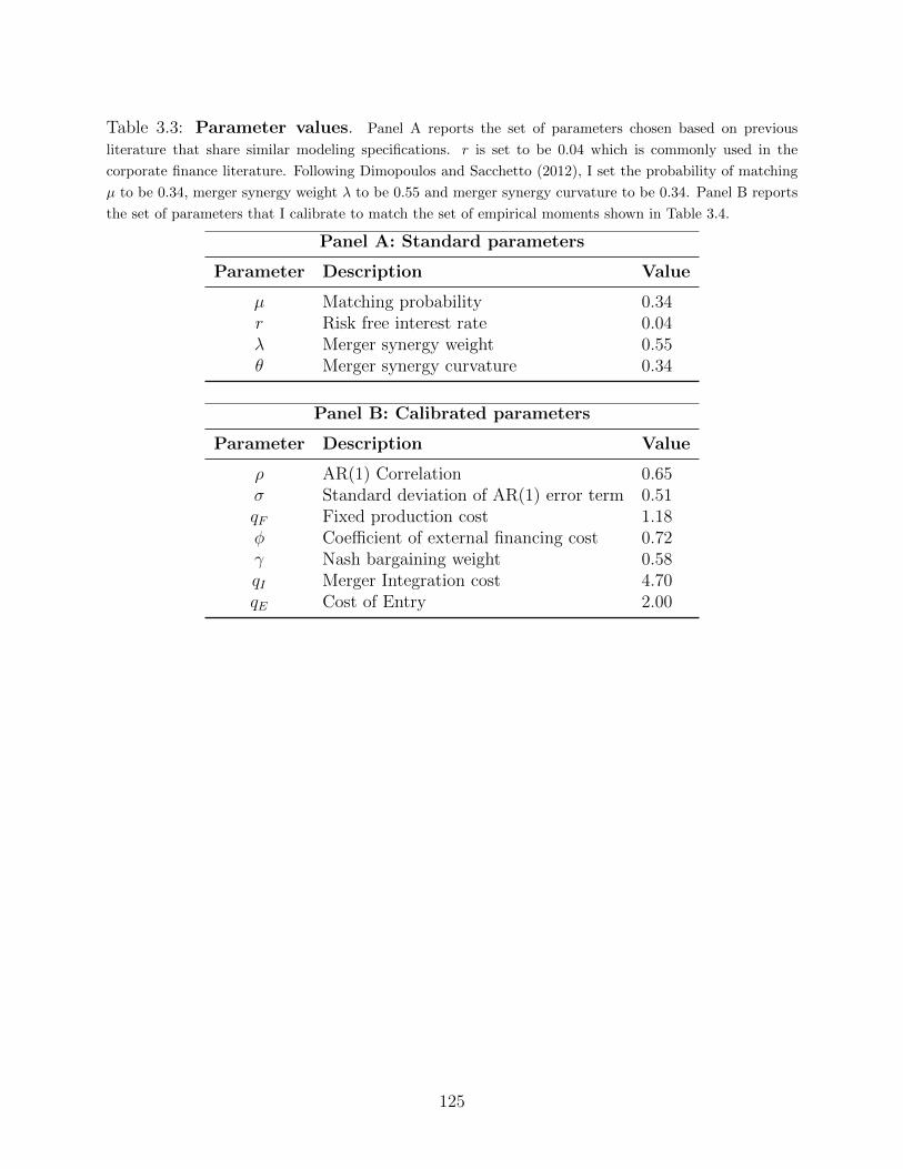
Table 3.3: Parameter values. Panel A reports the set of parameters chosen based on previous

literature that share similar modeling specifications. r is set to be 0.04 which is commonly used in the

corporate finance literature. Following Dimopoulos and Sacchetto (2012), I set the probability of matching

µ to be 0.34, merger synergy weight λ to be 0.55 and merger synergy curvature to be 0.34. Panel B reports

the set of parameters that I calibrate to match the set of empirical moments shown in Table 3.4.

Panel A: Standard parameters

Parameter Description Value

µ Matching probability 0.34r Risk free interest rate 0.04λ Merger synergy weight 0.55θ Merger synergy curvature 0.34

Panel B: Calibrated parameters

Parameter Description Value

ρ AR(1) Correlation 0.65σ Standard deviation of AR(1) error term 0.51qF Fixed production cost 1.18φ Coefficient of external financing cost 0.72γ Nash bargaining weight 0.58qI Merger Integration cost 4.70qE Cost of Entry 2.00

125

Table 3.4: Calibration.This table contains the empirical moments that I target in calibration and

their simulated counterparts. Defined on individual firms, the three moments ACSR, ACHR and AVD are

actually two dimensional average: average over firms in a certain period firm and then average over time. The

values of four empirical moments including AAR, AEXR, AENR and standard deviation of acquisition rate

are taken from Dimopoulos and Sacchetto (2012). I can see that simulated moments match their empirical

targets well except standard deviation of acquisition rate, and the firms in the simulated economy on average

hold less cash than in real life.

Variable Data Model

Average Cash Saving Rate (ACSR) 35.0% 23.3%Average Cash Holding Rate (ACHR) 67.2% 43.7%Average Acquisition Rate (AAR) 4.54% 4.51%Standard Deviation of Acquisition Rate 0.016 0.006Average Exit Rate (AEXR) 3.68% 3.70%Average Entry Rate (AENR) 8.22% 8.21%Average Value Difference (AVD) 0.859 0.852

126

Tab

le3.

5:Sim

ula

ted

finan

cial

chara

cteri

stic

sof

diff

ere

nt

kin

ds

of

firm

s.T

his

tab

leco

mp

are

the

fin

an

cial

chara

cter

isti

csof

firm

sin

the

sim

ula

ted

econ

omy

that

are

cate

gori

zed

inth

ree

way

s.T

he

six

vari

ab

les

incl

ud

edfo

rco

mp

ari

son

are

mea

nva

riab

les

that

firs

tly

aver

age

over

firm

sin

ace

rtai

np

erio

dan

dth

enav

erag

eti

me.

Fir

stof

all

,I

com

pare

acq

uir

ers,

targ

ets

an

dst

an

d-a

lon

efi

rms.

Ica

nfi

nd

that

acq

uir

ers

hav

e

hig

her

valu

eth

atst

and

-alo

nes

wh

ile

targ

ets

hav

elo

wer

-valu

eth

an

stan

d-a

lon

es,

an

dI

can

see

that

both

acq

uir

ers

an

dta

rget

son

aver

age

hold

more

cash

than

stan

d-a

lon

es.

Sec

ond,

Ico

mp

are

incu

mb

ents

an

den

trants

.I

fin

dth

at

incu

mb

ents

on

aver

age

are

sim

ilarl

ypro

du

ctiv

eas

entr

ants

,b

ut

incu

mb

ents

are

ofm

uch

hig

her

firm

valu

eb

ecau

seth

eyh

old

cash

wh

ile

entr

ants

do

not.

Fin

all

y,I

com

pare

stay

ing

firm

san

dex

itin

gfi

rms.

Sta

yin

g

firm

sar

em

ore

pro

du

ctiv

ean

dh

old

mor

eca

shth

an

exit

ing

firm

s,an

dth

us

thei

rfi

rmva

lues

are

mu

chh

igh

erth

an

thei

rex

itin

gco

unte

rpart

s.

Acq

uir

ers

Targ

ets

Sta

nd-

Incu

mb

ents

Entr

ants

Sta

yin

gE

xit

ing

alo

nes

firm

sfirm

s

Avera

ge

valu

e6.

970.

923

3.59

13.

800

0.90

63.

962

-0.5

66A

vera

ge

pro

duct

ion

revenue

0.99

00.

780

1.76

41.

762

1.60

91.

813

0.39

2A

vera

ge

cash

0.66

40.

609

0.52

80.

528

00.

648

0.39

6A

vera

ge

next

peri

od

cash

0.42

20

0.53

10.

522

0.01

50.

650

0A

vera

ge

cash

savin

gra

te0.

344

00.

229

0.22

90.

004

0.28

60

Avera

ge

cash

hold

ing

rate

0.77

50.

871

0.43

20.

433

00.

511

1.12

4

127

Figure 3.2: Productivity synergy function. This figure shows the productivity synergy function

when the synergy weight coefficient λ = 0.55 and curvature coefficient θ = 0.34.

128

Figure 3.3: Average cash saving rate comparative statics. ACSR is increasing in µ because

the stand-alone proportion is decreasing in µ and both acquirers and targets hold more cash than stand-

alones on average. ACSR is increasing the ρ and σ because of the intensified acquisition activities caused by

increases in ρ and σ. ACSR is decreasing in qF because an increase in qF will lead to a decrease in targets’

values and thus reduce acquisition payments. ACSR is increasing φ because costly external financing provides

the motivation for firms to hold cash. ACSR is decreasing in qI because of the reduced acquisition activities

caused by an increase in qI .

129

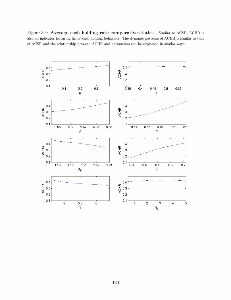
Figure 3.4: Average cash holding rate comparative statics . Similar to ACSR, ACHR is

also an indicator featuring firms’ cash holding behaviors. The dynamic patterns of ACHR is similar to that

of ACSR and the relationship between ACHR and parameters can be explained in similar ways.

130

Figure 3.5: Average acquisition rate comparative statics. AAR is almost linearly increasing

in µ because it is intuitive that more matchings implies more deals. AAR is increasing in ρ because synergy

benefit is increasing in ρ and AAR is increasing in σ because an increase in σ generates more diverse firm

production distribution. AAR is increasing in qF because an increase in qF reduces targets’ values. AAR is

decreasing in qI as an increase in qI implies higher acquisition cost, which results in less acquirers. AAR is

decreasing in qE since higher entry cost block potential entrants and reduce targets supply.

131

Figure 3.6: Average exit rate comparative statics. AEXR is decreasing in µ because getting

acquired is a substitution for firms to quit the market, and when chances of being acquired increase, original

exiting firms now become targets. AEXR is decreasing in ρ and σ because the increased acquisition activities

stimulated by increases in ρ and σ. AEXR is increasing in qF as higher fixed production cost leads to lower

continuation values. AEXR is increasing in φ and qI because increases in these two parameters causes

increases in acquisition costs, suppressing acquisitions and inducing more exits.

132

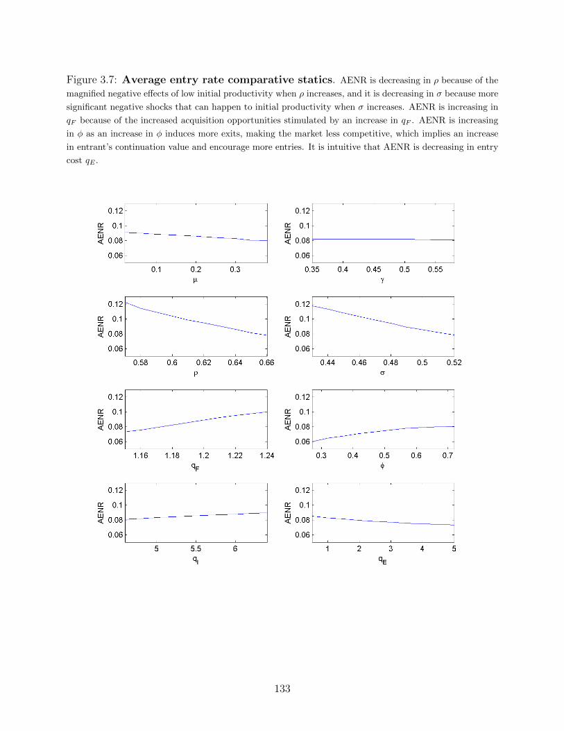
Figure 3.7: Average entry rate comparative statics. AENR is decreasing in ρ because of the

magnified negative effects of low initial productivity when ρ increases, and it is decreasing in σ because more

significant negative shocks that can happen to initial productivity when σ increases. AENR is increasing in

qF because of the increased acquisition opportunities stimulated by an increase in qF . AENR is increasing

in φ as an increase in φ induces more exits, making the market less competitive, which implies an increase

in entrant’s continuation value and encourage more entries. It is intuitive that AENR is decreasing in entry

cost qE .

133

Figure 3.8: Average value difference comparative statics. AVD is decreasing in µ, ρ and σ

because the standard deviation of normalized acquirers’ values decreases when more firms become acquirers

when there are increases in µ, ρ or σ. AVD is increasing in γ because when there is an increase in γ, matching

pairs with small differences in values which make acquisitions originally now do not make acquisitions any

more. AVD is increasing in qF because an increase in qF leads to decreases in values of both acquirers

and targets, but target values decrease more. AVD is increasing in entry cost qE because an increase in qE

discourages entry and reduces the probability that a firm will be match with an entrant which generally has

much lower value than incumbents.

134

Bibliography

Acharya, V., Almeida, H., Campello, M., 2007. Is cash negative debt? a hedging perspective on

corporate financial policies. Journal of Financial Intermediation 16, 515–554. 3.1

Ang, A., Bekaert, G., 2007. Stock return predictability: Is it there? Review of Financial studies

20, 651–707. 2.1

Ang, A., Hodrick, R. J., Xing, Y., Zhang, X., 2006. The cross-section of volatility and expected

returns. The Journal of Finance 61, 259–299. 1.1, 1.4.4, 1.4.5, 1.5.1

Bengio, Y., Schwenk, H., Senecal, J.-S., Morin, F., Gauvain, J.-L., 2006. Neural probabilistic

language models. In: Innovations in Machine Learning , Springer, pp. 137–186. 2.2

Blei, D. M., Ng, A. Y., Jordan, M. I., 2003. Latent dirichlet allocation. the Journal of machine

Learning research 3, 993–1022. 1.3, 2.4.4

Boldrin, M., Christiano, L. J., Fisher, J. D., 2001. Habit persistence, asset returns, and the business

cycle. American Economic Review pp. 149–166. 2.5

Brands, S., Brown, S. J., Gallagher, D. R., 2005. Portfolio concentration and investment manager

performance*. International Review of Finance 5, 149–174. 2.1

Brown, S. V., Tucker, J. W., 2011. Large-sample evidence on firms’ year-over-year md&a

modifications. Journal of Accounting Research 49, 309–346. 1.4.1

Campbell, J. Y., 1999. Asset prices, consumption, and the business cycle. Handbook of

macroeconomics 1, 1231–1303. 2.5

135

Campbell, J. Y., Shiller, R. J., 1988. The dividend-price ratio and expectations of future dividends

and discount factors. Review of financial studies 1, 195–228. 2.5

Campbell, J. Y., Yogo, M., 2006. Efficient tests of stock return predictability. Journal of financial

economics 81, 27–60. 2.1

Carhart, M. M., 1997. On persistence in mutual fund performance. The Journal of finance 52,

57–82. 1.1, 2.3.2

Cochrane, J. H., 2008. The dog that did not bark: A defense of return predictability. Review of

Financial Studies 21, 1533–1575. 2.5

Cochrane, J. H., 2011. Presidential address: Discount rates. The Journal of Finance 66, 1047–1108.

2.1, 2.3.2

Collobert, R., Weston, J., 2008. A unified architecture for natural language processing: Deep

neural networks with multitask learning. In: Proceedings of the 25th international conference on

Machine learning , ACM, pp. 160–167. 2.2

Cremers, K. M., Petajisto, A., 2009. How active is your fund manager? a new measure that predicts

performance. Review of Financial Studies p. hhp057. 2.1

Cremers, M., Halling, M., Weinbaum, D., 2015. Aggregate jump and volatility risk in the cross-

section of stock returns. The Journal of Finance 70, 577–614. 1.5.1

David, J., 2011. The aggregate implications of mergers and acquisitions. Working Paper. Available

at SSRN 2033555 . 3.1

Dimopoulos, T., Sacchetto, S., 2012. Merger activity in industry equilibrium. GSIA Working Papers

2012-E47, Carnegie Mellon University, Tepper School of Business. 3.1, 3.2, 3.2, 3.3.1, 3.3.2, 3.3,

3.4

Dow, J., da Costa Werlang, S. R., 1992. Uncertainty aversion, risk aversion, and the optimal choice

of portfolio. Econometrica: Journal of the Econometric Society pp. 197–204. 2.5

136

Dumais, S. T., 2004. Latent semantic analysis. Annual review of information science and technology

38, 188–230. 2.4.4

Edwards, F. R., Caglayan, M. O., 2001. Hedge fund performance and manager skill. Journal of

Futures Markets 21, 1003–1028. 2.1

Fama, E. F., French, K. R., 1988. Dividend yields and expected stock returns. Journal of financial

economics 22, 3–25. 2.1, 2.3.2

Fama, E. F., French, K. R., 1993. Common risk factors in the returns on stocks and bonds. Journal

of financial economics 33, 3–56. 1.1, 1.4.1, 1.5, 1.7, 1.3, 1.4, 2.3.2

Fama, E. F., French, K. R., 2001. Disappearing dividends: changing firm characteristics or lower

propensity to pay? Journal of Financial economics 60, 3–43. 1.4.1

Fama, E. F., French, K. R., 2015. A five-factor asset pricing model. Journal of Financial Economics

116, 1–22. 1.4.6, 1.7

Fama, E. F., MacBeth, J. D., 1973. Risk, return, and equilibrium: Empirical tests. The Journal of

Political Economy pp. 607–636. 1.1, 1.7

Fazzari, S. M., Hubbard, R. G., Petersen, B. C., Blinder, A. S., Poterba, J. M., 1988. Financing

constraints and corporate investment. Brookings Papers on Economic Activity 1988, pp. 141–206.

3.1

Gentzkow, M., Shapiro, J. M., 2006. What drives media slant? evidence from us daily newspapers.

Tech. rep., National Bureau of Economic Research. 1.3

Han, S., Qiu, J., 2007. Corporate precautionary cash holdings. Journal of Corporate Finance 13,

43–57. 3.1

Harford, J., 1999. Corporate cash reserves and acquisitions. The Journal of Finance 54, 1969–1997.

3.1

Heer, B., Maussner, A., 2009. Dynamic general equilibrium modeling: computational methods and

applications. Springer. 3.A.1

137

Huang, D., 2015. Gold, platinum, and expected stock returns. Tech. rep. 1.5.1

Jegadeesh, N., Titman, S., 1993. Returns to buying winners and selling losers: Implications for

stock market efficiency. The Journal of finance 48, 65–91. 1.4.5

Jegadeesh, N., Wu, D., 2013. Word power: A new approach for content analysis. Journal of Financial

Economics 110, 712–729. 2.1, 2.4.4

Kacperczyk, M., NIEUWERBURGH, S. V., Veldkamp, L., 2014. Time-varying fund manager skill.

The Journal of Finance 69, 1455–1484. 2.1

Kogan, S., Levin, D., Routledge, B. R., Sagi, J. S., Smith, N. A., 2009. Predicting risk from financial

reports with regression. In: Proceedings of Human Language Technologies: The 2009 Annual

Conference of the North American Chapter of the Association for Computational Linguistics,

Association for Computational Linguistics, pp. 272–280. 1.1, 1.4.1, 2.1, 2.3.1

Le, Q. V., Mikolov, T., 2014. Distributed representations of sentences and documents. arXiv

preprint arXiv:1405.4053 . 2.2.1

Lettau, M., Ludvigson, S., 2001. Consumption, aggregate wealth, and expected stock returns. the

Journal of Finance 56, 815–849. 2.3.2

Levy, O., Goldberg, Y., 2014. Neural word embedding as implicit matrix factorization. In: Advances

in Neural Information Processing Systems, pp. 2177–2185. 2.2.1, 2.2.2

Li, F., 2010. The information content of forward-looking statements in corporate filings–a naıve

bayesian machine learning approach. Journal of Accounting Research 48, 1049–1102. 1.1

Loughran, T., McDonald, B., 2011. When is a liability not a liability? textual analysis, dictionaries,

and 10-ks. The Journal of Finance 66, 35–65. 1.1, 2.1, 2.4.4, 2.4, 2.4

Manela, A., 2014. The value of diffusing information. Journal of Financial Economics 111, 181–199.

1.3

Mcauliffe, J. D., Blei, D. M., 2008. Supervised topic models. In: Advances in neural information

processing systems, pp. 121–128. 1.3

138

McLean, R. D., Pontiff, J., 2014. Does academic research destroy stock return predictability? In:

AFFI/EUROFIDAI, Paris December 2012 Finance Meetings Paper . 1.1, 1.3

Mikolov, T., Chen, K., Corrado, G., Dean, J., 2013a. Efficient estimation of word representations

in vector space. arXiv preprint arXiv:1301.3781 . 2, 2.1, 2, 2.2, 2.2.2, 2.6

Mikolov, T., Sutskever, I., Chen, K., Corrado, G. S., Dean, J., 2013b. Distributed representations

of words and phrases and their compositionality. In: Advances in neural information processing

systems, pp. 3111–3119. 2, 2.2, 2.2.1, 2.4.1

Mnih, A., Hinton, G. E., 2009. A scalable hierarchical distributed language model. In: Advances in

neural information processing systems, pp. 1081–1088. 2.2

Morellec, E., Nikolov, B., 2009. Cash holdings and competition. Working Paper. Available at SSRN

1364009 . 3.1

Morellec, E., Zhdanov, A., 2005. The dynamics of mergers and acquisitions. Journal of Financial

Economics 77, 649–672. 3.1

Newey, W. K., West, K. D., 1986. A simple, positive semi-definite, heteroskedasticity and

autocorrelationconsistent covariance matrix. 2.5, 2.5

Newey, W. K., West, K. D., 1987. Hypothesis testing with efficient method of moments estimation.

International Economic Review pp. 777–787. 1.2, 1.8, 1.9, 1.10

Nikolov, B., Schmid, L., Steri, R., 2013. Dynamic corporate liquidity. Working Paper. Available at

SSRN 2232538 . 3.1

Opler, T., Pinkowitz, L., Stulz, R., Williamson, R., 1997. The determinants and implications of

corporate cash holdings. Tech. rep., National Bureau of Economic Research. 3.1

Pastor, L., Stambaugh, R. F., 2001. Liquidity risk and expected stock returns. Tech. rep., National

Bureau of Economic Research. 1.1

Pastor, L., Stambaugh, R. F., 2009. Predictive systems: Living with imperfect predictors. The

Journal of Finance 64, 1583–1628. 2.5

139

Pinkowitz, L., Dahiya, E., Dastidar, P., Harford, J., Karolyi, A., Williamson, R., Zenner, M., 2002.

The market for corporate control and corporate cash holdings . 3.1

Rehurek, R., Sojka, P., 2010. Software Framework for Topic Modelling with Large Corpora. In:

Proceedings of the LREC 2010 Workshop on New Challenges for NLP Frameworks, ELRA,

Valletta, Malta, pp. 45–50. 2.4.1

Taddy, M., 2013. Multinomial inverse regression for text analysis. Journal of the American

Statistical Association 108, 755–770. 1.1, 1.3, 1.3, 1.3, 1.3

Tang, D., Wei, F., Yang, N., Zhou, M., Liu, T., Qin, B., 2014. Learning sentiment-specific word

embedding for twitter sentiment classification. In: ACL (1), pp. 1555–1565. 2.2

Tetlock, P. C., 2007. Giving content to investor sentiment: The role of media in the stock market.

The Journal of Finance 62, 1139–1168. 1.1, 1.3, 2.1, 2.4.4

Tetlock, P. C., SAAR-TSECHANSKY, M., Macskassy, S., 2008. More than words: Quantifying

language to measure firms’ fundamentals. The Journal of Finance 63, 1437–1467. 2.4.4

Turian, J., Ratinov, L., Bengio, Y., 2010. Word representations: a simple and general method

for semi-supervised learning. In: Proceedings of the 48th annual meeting of the association for

computational linguistics, Association for Computational Linguistics, pp. 384–394. 2.2

Van der Maaten, L., Hinton, G., 2008. Visualizing data using t-sne. Journal of Machine Learning

Research 9, 85. 2.4.2

Vassalou, M., 2003. News related to future gdp growth as a risk factor in equity returns. Journal

of financial economics 68, 47–73. 1.1

140