applications of linear and nonlinear robustness analysis techniques to the f/a-18 flight control

Applications of Linear and Nonlinear Robustness

Analysis Techniques to the F/A-18 Flight Control Laws

Abhijit Chakraborty ∗ and Peter Seiler † and Gary J. Balas‡

Department of Aerospace Engineering & Mechanics, University of Minnesota , Minneapolis, MN, 55455, USA

The F/A-18 Hornet aircraft with the original flight control law exhibited an out-of-control phenomenon known as the falling leaf mode. Several aircraft were lost due tothe falling leaf mode and which led NAVAIR and Boeing to redesign the flight controllaw. The revised flight control law successfully suppressed the falling leaf mode duringflight tests with aggressive maneuvers. This paper compares the robustness of the original(baseline) and revised control laws using linear analyses, Monte Carlo simulations, andnonlinear region-of-attraction analyses. The linear analyses indicate the revised controlleronly marginally improves the closed-loop robustness while the nonlinear analyses indicatea substantial improvement in robustness over the baseline controller. This example demon-strates the potential for nonlinear analyses to detect out-of-control phenomenon that arenot evident from linear analyses.

Nomenclature

α Angle-of-attack, radβ Sideslip Angle, radVT Velocity, ft/sp Roll rate, rad/sq Pitch rate, rad/sr Yaw rate, rad/sφ Bank angle, radθ Pitch angle, radψ Yaw angle, radT Thrust, lbfρ Density, slugs/ft3

q 12ρV

2T : Dynamic pressure

V Lyapunov Functionm Mass, slugsIC Initial Condition

I. Introduction

The US Navy F/A-18 A/B/C/D Hornet aircraft with the original baseline flight control law experienced anumber of out-of-control flight departures since the early 1980’s. Many of these incidents have been describedas a falling leaf motion of the aircraft.1 The falling leaf motion has been studied extensively to investigate theconditions that lead to this behavior. The complex dynamics of the falling leaf motion and lack of flight datafrom the departure events pose a challenge in studying this motion. An extensive revision of the baselinecontrol law was performed by NAVAIR and Boeing in 2001 to suppress departure phenomenon, improve∗Graduate Research Assistant: [email protected].†Senior Research Associate: [email protected].‡Professor: [email protected].

1 of 25

American Institute of Aeronautics and Astronautics

AIAA Guidance, Navigation, and Control Conference10 - 13 August 2009, Chicago, Illinois

AIAA 2009-5675

Copyright © 2009 by Abhijit Chakraborty. Published by the American Institute of Aeronautics and Astronautics, Inc., with permission.

maneuvering performance and to expand the flight envelope.1 The revised control law was implemented onthe F/A-18 E/F Super Hornet aircraft after successful flight tests. These flight tests included aggressivemaneuvers that demonstrated successful suppression of the falling leaf motion by the revised control law.

It is of practical interest to compare the robustness of the baseline and revised flight controllers. Oneobjective of this paper is to use linear analyses, Monte Carlo simulations, and nonlinear region of attractionanalyses to compare the robustness guarantees of each of the design. Region-of-attraction analysis fornonlinear systems provides a guaranteed stability region using Lyapunov theory and recent results in sum-of-squares optimization.2–6 This is complementary to the use of Monte Carlo simulations to search for unstabletrajectories. The sums-of-squares stability analysis has previously been applied to simple examples,2–6

though this is the first application of these techniques to an actual industry flight control problem. Thesecond objective is to use the nonlinear region-of-attraction technique to analyze and draw conclusionsabout the F/A-18 aircraft flight control system. Nonlinear analysis is necessary as the falling leaf motion isdue to nonlinearities in the aircraft dynamics and cannot be replicated in simulation by linear models. Thismakes the falling leaf motion a particularly interesting example for the application of nonlinear robustnessanalysis techniques.

The remainder of the paper has the following outline. Section II describes the characteristics of thefalling leaf motion. Section III provides a brief description of the F/A-18 aircraft including its aerodynamiccharacteristics and equations of motion. The baseline and revised flight control laws are described in SectionIV. Section V provides a comparison of the closed-loop robustness properties with the baseline and revisedflight control laws. This section includes both the linear and nonlinear analyses for each control law. Asummary of results and comparisons between linear robustness and nonlinear analyses techniques is alsopresented in Section V. Finally a brief conclusion is given in Section VI. All data required to reproduce theresults presented in this paper are provided in the Appendices.

II. Falling Leaf Motion

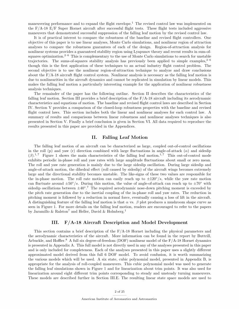
The falling leaf motion of an aircraft can be characterized as large, coupled out-of-control oscillationsin the roll (p) and yaw (r) direction combined with large fluctuations in angle-of-attack (α) and sideslip(β).1,7 Figure 1 shows the main characteristics of the falling leaf motion.1,7 This out-of-control modeexhibits periodic in-phase roll and yaw rates with large amplitude fluctuations about small or zero mean.The roll and yaw rate generation is mainly due to the large sideslip oscillation. During large sideslip andangle-of-attack motion, the dihedral effect (roll caused by sideslip) of the aircraft wings becomes extremelylarge and the directional stability becomes unstable. The like-signs of these two values are responsible forthe in-phase motion. The roll rate motion can easily reach up to ±120/s, while the yaw rate motioncan fluctuate around ±50/s. During this motion, the value of angle-of-attack can reach up to ±70 withsideslip oscillations between ±40.7 The required aerodynamic nose-down pitching moment is exceeded bythe pitch rate generation due to the inertial coupling of the in-phase roll and yaw rates. The reduction inpitching moment is followed by a reduction in normal force, eventually causing a loss of lift in the aircraft.A distinguishing feature of the falling leaf motion is that α vs. β plot produces a mushroom shape curve asseen in Figure 1. For more details on the falling leaf motion, readers are encouraged to refer to the papersby Jaramillo & Ralston7 and Heller, David & Holmberg.1

III. F/A-18 Aircraft Description and Model Development

This section contains a brief description of the F/A-18 Hornet including the physical parameters andthe aerodynamic characteristics of the aircraft. More information can be found in the report by Buttrill,Arbuckle, and Hoffler.8 A full six degree-of-freedom (DOF) nonlinear model of the F/A-18 Hornet dynamicsis presented in Appendix A. This full model is not directly used in any of the analyses presented in this paperand is only included for completeness. Each of the analyses presented in this paper uses a slightly differentapproximated model derived from this full 6 DOF model. To avoid confusion, it is worth summarizingthe various models which will be used. A six state, cubic polynomial model, presented in Appendix B, isappropriate for the analysis of roll-coupled maneuvers. This cubic polynomial model was used to generatethe falling leaf simulations shown in Figure 1 and for linearization about trim points. It was also used forlinearization around eight different trim points corresponding to steady and unsteady turning maneuvers.These models are described further in Section III.E. The resulting linear state space models are used to

2 of 25


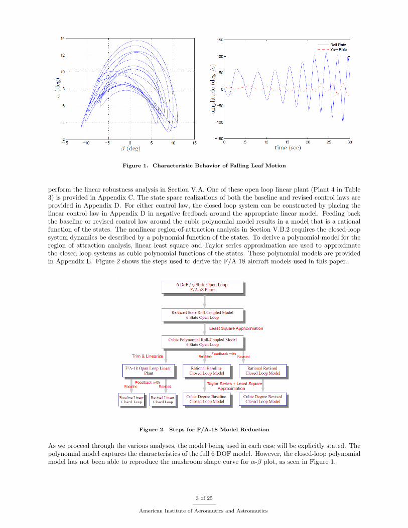
Figure 1. Characteristic Behavior of Falling Leaf Motion

perform the linear robustness analysis in Section V.A. One of these open loop linear plant (Plant 4 in Table3) is provided in Appendix C. The state space realizations of both the baseline and revised control laws areprovided in Appendix D. For either control law, the closed loop system can be constructed by placing thelinear control law in Appendix D in negative feedback around the appropriate linear model. Feeding backthe baseline or revised control law around the cubic polynomial model results in a model that is a rationalfunction of the states. The nonlinear region-of-attraction analysis in Section V.B.2 requires the closed-loopsystem dynamics be described by a polynomial function of the states. To derive a polynomial model for theregion of attraction analysis, linear least square and Taylor series approximation are used to approximatethe closed-loop systems as cubic polynomial functions of the states. These polynomial models are providedin Appendix E. Figure 2 shows the steps used to derive the F/A-18 aircraft models used in this paper.

Figure 2. Steps for F/A-18 Model Reduction

As we proceed through the various analyses, the model being used in each case will be explicitly stated. Thepolynomial model captures the characteristics of the full 6 DOF model. However, the closed-loop polynomialmodel has not been able to reproduce the mushroom shape curve for α-β plot, as seen in Figure 1.

3 of 25


A. Physical Parameters

Figure 3. F/A-18 Hornet

The F/A-18 Hornet aircraft, Figure 3a, is a high performance, twin engine fighter aircraft built by theMcDonnell Douglas (currently known as the ‘Boeing’) Corporation. Each engine is a General Electric, F404-GE-400 rated at 16,100-lbf of static thrust at sea level. The aircraft features a low sweep trapezoidal wingplanform with 400 ft2 area and twin vertical tails.8 Table 1 lists the aerodynamic reference and physicalparameters of the aircraft.

Table 1. Aircraft Parameters

Wing Area, Sref 400 ft2

Mean Aerodynamic Chord (c) 11.52 ftWing Span, bref 37.42 ft

Mass, m 1034.5 slugsIxx 23000 slug-ft2

Iyy 151293 slug-ft2

Izz 169945 slug-ft2

Ixz -2971 slug-ft2

B. Control Surfaces

The conventional F/A-18 Hornet aircraft has five pairs of control surfaces: stabilators, rudders, ailerons,leading edge flaps, and trailing edge flaps. However, only the symmetric stabilator, differential aileron anddifferential rudder are considered as control effectors for the analyses performed in this paper. Longitudinalcontrol or pitch control is provided by the symmetric deflection of the stabilators. Deflection of differen-tial ailerons is used to control the roll or lateral direction, while differential deflection of rudders providedirectional or yaw control. The actuation systems for these primary controls are modeled as first order lags.Table 2 provides the mathematical models of the actuators and their deflection and rate limits.8 However,the actuators’ dynamics and rate/position limits are neglected for all analyses. Their values are only includedfor completeness.

Table 2. Control Surface and Actuator Configuration

Actuator Rate Limit Position Limit ModelStabilator, δstab ±40/s -24,+10.5 30

s+30

Aileron, δail ±100/s -25,+45 48s+48

Rudder, δrud ±61/s -30,+30 40s+40

aPictures taken from http://www.dfrc.nasa.gov/Gallery/Photo/F-18Chase/Large/EC96-43830-11.jpg

4 of 25


C. Equations of Motion & Aerodynamic Model

The conventional aircraft equations of motion described in Stengel,9 Cook,10 and Napolitano and Spagnuolo11

are primarily driven by the aerodynamic forces and moments acting on the aircraft. In this paper, we followthe notation used in the report by Napolitano and Spagnuolo.11 The equations of motion for the 6 DOF fullmodel are presented in the Appendix A. The two aerodynamic angles, angle-of-attack (α) and sideslip angle(β), are needed to specify the aerodynamic forces and moments. These aerodynamic forces and momentsalso depend on the angular rates and the deflection of the control surfaces. The longitudinal coefficients (lift,drag, and pitching moment) primarily depend on the angle-of-attack (α); in the lateral directional coefficients(roll, yaw, and sideforce), sideslip angle (β) is equally as important as α.12 Many flight experiments havebeen performed to estimate the stability and control derivatives of the F/A-18 High Alpha Research Vehicle(HARV).13–16 The F/A-18 HARV has similar aerodynamic characteristics as the F/A-18 Hornet17 with theexception of the F/A-18 HARV having thrust vectoring control. Hence, we will use the F/A-18 HARVaerodynamic data to represent the F/A-18 aircraft in all models that are presented in this paper. Theaerodynamic model for the full six degree-of-freedom model is presented in the Appendix A.

D. Reduced Equations of Motion

The nonlinear region of attraction analysis3 requires the aircraft dynamics to be described by a polynomialmodel. The computational burden of the analysis also restricts the polynomial degree to be less than orequal to 3. Hence, a six state cubic polynomial model of the F/A-18 aircraft for roll-coupled maneuvers18 isused in this paper for performing all the analyses. The reduced (open loop cubic polynomial) equations ofmotion are presented in the Appendix B.

The polynomial model described in the Appendix B captures the characteristics of the full 6 DOF modelpresented in Appendix A. During this OCF motion, the velocity is usually on the order of 250 ft/s.7 In thispaper, the velocity is assumed to be constant, and equal to 250 ft/s. Aggressive maneuvers, like bank turn,are more likely to put the aircraft in the falling leaf motion compared to straight and level flight. Hence, weconsider a steady bank turn maneuver of the aircraft with zero climb rate (θ = 0). This assumption allowsthe pitch angle (θ) and yaw angle (ψ) to be ignored, resulting in a six state model. Thrust effects in thesideslip direction are also neglected. Small angle approximations are used for the trigonometric terms in thefull 6 DOF model to derive a polynomial representation of the aircraft dynamics. Finally, we perform leastsquares fit of the aerodynamic data over a gridded α - β space of −20 ≤ β ≤ 20, and −10 ≤ α ≤ 40 torestrict the description of the dynamics up to cubic degree.

E. Formulation of Linear Models

The cubic polynomial model, presented in Appendix B, is linearized around steady (β = 0) and unsteady(β = 10o) turning maneuvers for different bank angles (φ). Steady bank turn is a usual maneuver for anyaircraft. However, wind disturbances or any upset conditions can force the aircraft to perform unsteadybank turn maneuvers. Hence, we will consider both scenarios. Aggressive maneuvers, like large bank turn(i.e, φ = 60o), are more likely to put the aircraft into the falling leaf motion compared to straight and levelflight. Longitudinal and lateral direction become highly coupled during such maneuvers. Hence, linearizationaround such maneuvers will result in linear models which may be well suited to capture the coupling effect ofthe aircraft which is one of the important causes for initiating the falling leaf motion.7 It is of considerableinterest to perform linear robustness comparison between the baseline and revised flight control law. Theoperating points for formulating the linear models are presented in Table 3. All the linear aircraft models aretrimmed around the flight condition of: VT = 250 ft/s, altitude =25, 000 ft, and α = 26o. We will performthe nonlinear analysis around the trim condition listed for Plant 4 in Table 3. Only Plant 4 and Plant 8 areconsidered for loopmargin analysis. In addition, all eight plants, mentioned in Table 3, are used to performthe linear robustness (µ) analysis as presented in Section V.A.

IV. Control Law Design

This section provides an overview of both the baseline and revised control laws. In both cases, the controllaws are divided into three channels: longitudinal, lateral, and directional.

5 of 25


Table 3. Trim Values around VT = 250 fts

altitude =25, 000 ft, and α = 26o

State/Input Plant 1 Plant 2 Plant 3 Plant 4 Plant 5 Plant 6 Plant 7 Plant 8Sideslip, β 0 0 0 0 10 10 10 10

Bank Angle, φ 0 25 45 60 0 25 45 60

Roll Rate, p 0/s 0/s 0/s 0/s 0/s 0/s 0/s 0/sYaw Rate, r 0/s 3.20/s 5.78/s 7.70/s 0.069/s 3.28/s 5.84/s 7.77/sPitch Rate, q 0/s 0/s 0/s 0/s 0/s 0/s 0/s 0/s

δStab -21.78 -21.78 -21.78 -21.78 -21.78 -21.78 -21.78 -21.78

δAil 0 0.31 0.56 0.75 19.68 19.98 20.24 20.42

δRud 0 -2.37 -4.27 -5.69 3.32 0.96 -0.94 -2.36

T (lbf) 36464 36464 36464 36464 36464 36464 36464 36464

A. Baseline Control Law

Figure 4 shows the control law architecture for the baseline control laws used for analysis in this paper.The baseline controller structure for the F/A-18 aircraft closely follows the Control Augmentation System(CAS) presented in the report by Buttrill, Arbuckle, and Hoffler.8 The actuator (Astab, Arud, Aail) dynamics,presented in Table 2, are neglected for analysis purposes, i.e. Astab = Arud = Aail = 1. Any differencesbetween the control structure presented here and in the report by Buttrill, Arbuckle, and Hoffler8 is describedin the following sections.

Actuator

Actuator

Actuator

8

0.5

-0.8

0.8

Longitudinal

Lateral

Directional F/A-18 Plant

Figure 4. F/A-18 Baseline Flight Control Law

1. Longitudinal Control

The longitudinal baseline control design for the F/A-18 aircraft includes angle-of-attack (α in rad), normalacceleration (an in g), and pitch rate (q in rad/s) feedback. The angle-of-attack feedback is used to stabilizean unstable short-period mode that occurs during low speed, high angle-of-attack maneuvering. The inner-loop pitch rate feedback is comprised of a proportional feedback gain, to improve damping of the short-period

6 of 25


mode. In the high speed regime, this feedback gain needs to be high to avoid any unstable short-period mode.The normal acceleration feedback, a proportional-integrator (PI) compensator, has not been implementedin our analysis since only roll-coupled maneuvers are considered.

2. Lateral Control

Control of the lateral direction axis involves roll rate (p in rad/s) feedback to the aileron actuators. Roll ratefeedback is used to improve roll damping and the roll-subsidence mode of the aircraft. Due to the inherenthigh roll damping associated with the F/A-18 aircraft at high speed, the roll rate feedback authority isusually reduced at high dynamic pressure. In the low speed regime, the roll rate feedback gain is increasedto improve the Dutch roll damping. The roll rate feedback gain ranges between 0.8 at low speed to 0.08 athigh speed. At 250 ft/s, flight condition described in this paper, a feedback gain of 0.8 is used to provideroll damping.

3. Directional Control

Directional control involves feedback from yaw rate (r in rad/s) and lateral acceleration (ay in g) to therudder actuators. Yaw rate is fed back to the rudder to generate a yawing moment. Yaw rate feedbackreduces yaw rate contribution to the Dutch-roll mode. In a steady state turn, there is always a constantnonzero yaw rate present. This requires the pilot to apply larger than normal rudder input to negate theeffect of the yaw damper and make a coordinated turn. Hence, a washout filter is used to effectively eliminatethis effect. The filter approximately differentiates the yaw rate feedback signal at low frequency, effectivelyeliminating yaw rate feedback at steady state conditions.12 The lateral acceleration feedback contributes toreduce sideslip during turn coordination.

B. Revised Control Law

Actuator

Actuator

Actuator

8

0.5

-0.8

0.8

Longitudinal

Lateral

Directional F/A-18 Plant

-0.5

-2

Figure 5. F/A-18 Revised Flight Control Law

Figure 5 shows the architecture of the revised F/A-18 flight control law as described in the papers byHeller, David, & Holmberg1 and Heller, Niewoehner, & Lawson.19 The objective of the revised flight controllaw was to improve the departure resistance characteristics and full recoverability of the F/A-18 aircraftwithout sacrificing the maneuverability of the aircraft.1 The significant change in the revised control law

7 of 25


was the additional sideslip (β in rad) and sideslip rate (β in rad/s) feedback to the aileron actuators. Thesideslip feedback plays a key role in increasing the lateral stability in the 30− 35 range of angle-of-attack.The sideslip rate feedback improves the lateral-directional damping. Hence, sideslip motion is damped evenat high angles-of-attack. This feature is key to eliminating the falling leaf mode, which is an aggressive formof in-phase Dutch-roll motion. There are no direct measurements of sideslip and sideslip rate. Therefore,they are estimated for feedback. The sideslip and the sideslip rate feedback signals are computed based onalready available signals from the sensors and using the kinematics of the aircraft. Proportional feedbackhas been implemented for these two feedback channels. The values of the proportional gains are kβ = 0.5and kβ = 2.

V. Analysis

Linear robustness and nonlinear region-of-attraction analyses are performed to compare the baseline andthe revised F/A-18 flight control laws. The linear analysis captures the local behavior of the system andis only valid around the equilibrium point of the linearization. Linear analysis does not provide insightinto how the nonlinearities of the aircraft dynamics will affect the stability properties of the system. Twoapproaches are taken to analyze the effect of the nonlinearities. First, the closed-loop flight control systemsare analyzed by using region-of-attraction estimation techniques to compute an inner estimate of the stabilityboundaries. Second, Monte Carlo simulations are performed on the closed-loop dynamics to estimate outerbounds of the stability boundaries. The linear robustness analysis has been performed using the RobustControl Toolbox.20

A. Linear Analysis

The cubic polynomial model described in Appendix B is linearized around the flight condition of: VT = 250ft/s, altitude =25, 000 ft at different bank angle turn, i.e, φ = 0o, 25o, 45o, 60o. Section III.E presents theoperating points for the linear systems. The actuator states are excluded from both linear and nonlinearmodels. The actuators have very fast dynamics, as mentioned in Table 2, and their dynamics can be neglectedwithout causing any significant variation in the analysis results. Validation and verification of flight controllaw relies heavily on applying linear analysis at trim points throughout the flight envelope. Linear analysisusually amounts to investigating robustness issues and possible worst-case scenarios around the operatingpoints of interest.

1. Loopmargin Analysis

Gain and phase margins provide stability margins for the closed-loop system. Poor gain and phase marginsindicate poor robustness of the closed-loop system. A typical requirement for certification of a flight controllaw requires the closed-loop system to achieve at least 6dB of gain margin and 450 of phase margin. However,the classical loop-at-a-time SISO (Single-Input-Single-Output) margin can be unreliable for MIMO (Multi-Input-Multi-Output) systems. The F/A-18 aircraft closed- loop plants under consideration are multivariable;hence, we will perform both disk margin and multivariable margin analysis in addition to the classical loop-at-a-time margin analysis.

Classical Gain, Phase and Delay Margin Analysis: Classical gain, phase and delay margins providerobustness margins for each individual feedback channel with all the other loops closed. This loop-at-a-timemargin analysis provides insight on the sensitivity of each channel individually. Table 4 provides the classicalmargins for both the baseline and the revised flight control laws. The results, presented in Table 4, are basedon the unsteady (β = 10o) bank turn maneuver at φ = 60o (Plant 8). The baseline and revised flight controllaws have very similar classical margins at the input channel. However, loop-at-a-time margin analysis can beunreliable for a multivariable system. Hence, multivariable loop margin analysis is necessary to understandhow coupling between the channel effects the robustness properties.

Disk Margin Analysis: Disk margin analysis provides an estimate on how much combined gain/phasevariations can be tolerated at each channel with other loops closed. The disk margin metric is very similarto an exclusion region on a Nichols chart. As with the classical margin calculation, coupling effects betweenchannels may not be captured by this analysis. Table 5 provides the disk gain and phase variations at each

8 of 25


Table 4. Classical Gain & Phase Margin Analysis for Plant 8

Input Channel Baseline Revised

Aileron Gain Margin ∞ 27 dBPhase Margin 104o 93o

Delay Margin 0.81 sec 0.44 secRudder Gain Margin 34 dB 34 dB

Phase Margin 82o 76o

Delay Margin 2.23 sec 1.99 secStabilator Gain Margin ∞ ∞

Phase Margin 91o 91o

Delay Margin 0.24 sec 0.24 sec

loop for both the control laws. The results are based on the unsteady (β = 10o) bank turn maneuver atφ = 60o (Plant 8). The baseline flight control law achieves slightly better stability margins in the stabilatorchannel; while the revised flight control law has slightly better margins in the aileron channel. Overall, thedisk margins between the two flight control laws are nearly indistinguishable. Disk margin analysis has notprovided any definitive certificate on which of the two flight control law is more robust. The multivariable,simultaneous disk margin analysis across all channels may provide a better insight on which control law hasbetter margins.

Table 5. Disk Margin Analysis for Plant 8

Input Channel Baseline Revised

Aileron Gain Margin 20 dB ∞Phase Margin 78o 90o

Rudder Gain Margin 15 dB 14 dBPhase Margin 69o 67o

Stabilator Gain Margin ∞ ∞Phase Margin 90o 90o

Multivariable Disk Margin Analysis: The multivariable disk margin indicates how much simultaneous(across all channels), independent gain and phase variations can the closed-loop system tolerate beforebecoming unstable. This analysis is conservative since it allows independent variation of the input channelssimultaneously. Figure 6 presents the multivaribale disk margin ellipses. Figure 6(a) is based on Plant 4and Figure 6(b) is based on Plant 8. The mutivariable disk margin analysis certifies that for simultaneousgain & phase variations in each channel inside the region of the ellipses the closed-loop system remainsstable. The mutivariable disk margin analysis for steady bank turn maneuvers, in Figure 6(a), shows boththe baseline and the revised flight control laws have similar multivariable margins. For this steady maneuver,both the control laws can handle gain variation up to ≈ ±12.5 dB and phase variation of ≈ ±64o acrosschannels. Figure 6(b) shows the mutivariable disk margin analysis for unsteady bank turn maneuvers. Here,the revised flight control law achieves slightly better margin (Gain margin = ±11.3dB, Phase margin =±600) than the baseline flight control law ( Gain margin = ±9.5dB, Phase margin = ±540). However, thedifferences in the margins between the two control laws is not significant enough to conclude which flightcontrol law is susceptible to the falling leaf motion. Moreover, both the control laws achieve the typicalmargin requirement specification (6dB gain margin and 450 phase margin).

2. Input Multiplicative Uncertainty

Modeling physical systems perfectly is always a challenge. A mathematical model of the physical systemalways differs from the actual behavior of the system in many engineering problems. The F/A-18 aircraft

9 of 25


(a) Steady Maneuvers at φ = 60o (b) Unsteady Maneuvers at φ = 60o

Figure 6. Disk Margin Analysis of the Baseline and Revised F/A-18 Flight Control Law

Figure 7. F/A-18 Input Multiplicative Uncertainty Structure

model presented in this paper is no exception. One approach is to account for the inaccuracies of the modeledaircraft dynamics as input multiplicative uncertainty.

Figure 7 shows the general uncertainty structure of the plant that will be considered in the input multi-plicative uncertainty analysis. To assess the performance due to the inaccuracies of the modeled dynamics,we introduce multiplicative uncertainty, WI∆IM , in all four input channels. The uncertainty ∆IM representsunit norm bounded unmodeled dynamics. The weighting function will be set to unity for analysis purpose,WI = I4×4. We will perform the structured-singular-value (µ) analysis. The 1

µ value measures the stabilitymargin due to the uncertainty description in the system.

Diagonal Input Multiplicative Uncertainty: Figure 8 shows the µ plot of both the closed loops at bothsteady and unsteady bank maneuvers. The left subplot presents results based on plants 1-4, as mentioned inTable 3, for steady (β = 0) maneuvers, and the right subplot presents results based on plants 5-8 for unsteady(β = 10o) maneuvers. Here the uncertainty, ∆IM , has a diagonal structure. This models uncertainty ineach actuation channel but no cross-coupling between the channels. The value of µ at each frequency ω isinversely related to the smallest uncertainty which causes the feedback system to have poles at ±jω. Thusthe largest value on the µ plot is equal to 1/km where km denotes the stability margin. In Figure 8(a), thepeak value of µ is 0.97 (km = 1.03) for both the revised and baseline controller during steady maneuvers,which indicates a very robust flight control system. In addition, Figure 8(b) shows the peak value of µ forboth the control laws at unsteady bank turn maneuvers. Here, the baseline flight controller exhibits a peakµ value of 1.25 (km = 0.83) and the revised flight controller achieves a µ value of 1.20 (km = 0.80). In bothsteady and unsteady maneuvers, both the controllers achieve similar stability margins for diagonal inputmultiplicative uncertainty across the input channel. These results corresponds well with the classical margin

10 of 25


(a) Steady Maneuvers (b) Unsteady Maneuvers

Figure 8. Diagonal Input Multiplicative Uncertainty Analysis of the Baseline and Revised F/A-18 FlightControl Law

results in Section V.A.1 .

Full Block Input Multiplicative Uncertainty: Figure 9 shows the µ plot for both steady and unsteadymaneuvers. The left subplot presents results based on plants 1-4, as mentioned in Table 3, for steady (β = 0)maneuvers, and the right subplot presents results based on plants 5-8 for unsteady (β = 10o) maneuvers. Inthis analysis, ∆IM is allowed to be a full block uncertainty. This uncertainty structure models the effectsof dynamic cross-coupling between the channels to determine how well the flight control laws are able tohandle the coupling at the input to the F/A-18 actuators. As mentioned before, the falling leaf motion isan exaggerated form of in-phase Dutch-roll motion with large coupling in the roll-yaw direction. Increasedrobustness of the flight control law with respect to the full ∆IM is associated with its ability to mitigatethe onset of the falling leaf motion. Figure 9(a) shows the µ analysis for steady maneuvers. In this case,both the baseline and revised flight control law achieves similar stability margin (µ = 1.02 and km = 0.98).Figure 9(b) shows the µ analysis for unsteady maneuvers. Here, the baseline flight controller exhibits a peakµ value of 1.25 (km = 0.83) and the revised flight controller achieves a µ value of 1.20 (km = 0.80). Inboth steady and unsteady maneuvers, both the controllers achieve similar stability margins for full inputmultiplicative uncertainty across the input channels.

Robustness analysis with respect to input multiplicative uncertainty (both full block and diagonal) acrossinput channels has not detected any performance issue with the baseline flight control law compare to therevised flight control law. At this point, the linear analysis shows both controllers are very robust withsimilar stability margins and that should mitigate the onset of the falling leaf motion.

3. Robustness Analysis to Parametric Uncertainty

So far we have provided a stability analysis with respect to unstructured dynamic uncertainty at the modelinputs. Robustness analysis of flight control system with structured uncertainty is another important analysisin validating closed-loop robustness and performance.21 Moreover, robustness assessment of the flight controllaw due to the nonlinear variations of aerodynamic coefficients over the flight envelope needs to be considered.Including parametric uncertainty models into the analysis is one approach to address this issue. Bothcontrollers are examined with respect to robustness in the presence of parametric variations in the plantmodel. To this end, we represented the stability derivatives of the linearized model with ±10% uncertaintyaround their nominal values. These terms are chosen carefully to represent the stability characteristics of

11 of 25



Figure 9. Full Block Input Multiplicative Uncertainty Analysis of the Baseline and Revised F/A-18 FlightControl Law

the F/A-18 aircraft that play an important role in the falling leaf motion. These terms are related to theentries of the linearized open-loop A matrix. The terms in the lateral directions are: sideforce due to sideslip(Yβ); rolling moment due to sideslip (Lβ); yawing moment due to sideslip (Nβ); roll damping (Lp); yawdamping (Nr). The following longitudinal terms have also been considered: pitch damping (Mq); normalforce due to pitch rate (Zq); pitch stiffness (Mα). Cook10 provides a detailed description of these terms. Thelateral aerodynamic terms: Yβ , Lβ , Nβ , Lp, and Nr correspond respectively to the (1, 1), (2, 1), (3, 1), (2, 2),and (3, 3) entries of the linearized A matrix presented in previous section. The longitudinal aerodynamicterms: Mq, Zq, and Mα correspond respectively to the (6, 6), (5, 6), and (6, 5) entries of the same linearizedA matrix.

Figure 10 shows the µ plot (for both steady and unsteady maneuvers) of both closed-loop systems withrespect to this parametric uncertainty. Again, the left subplot presents results based on plants 1-4, asmentioned in Table 3, for steady (β = 0o) maneuvers, and the right subplot presents results based on plants5-8 for unsteady (β = 10o) maneuvers. For steady maneuvers, in Figure 10(a), the stability margin forparametric uncertainty in the aerodynamic coefficients of the revised controller (µ = 0.092 and km = 10.8) isapproximately 1.3 times larger than that of the baseline controller (µ = 0.115 and km = 8.7). For unsteadymaneuvers, in Figure 10(b), the stability margin for parametric uncertainty in the aerodynamic coefficientsof the revised controller (µ = 0.109 and km = 9.17) is approximately 1.2 times larger than that of thebaseline controller (µ = 0.131 and km = 7.63). Hence, the revised flight controller is more robust to error inaerodynamic derivatives than the baseline design, but overall both flight controllers are very robust designs.

To this point, the linear robustness analysis indicate both the revised and baseline flight control lawsare slightly less robust for unsteady maneuvers compared to the steady maneuvers. However, both thecontrol laws achieve similar robustness properties separately for steady and unsteady maneuvers. The linearrobustness analysis for the F/A-18 flight control laws do not indicate any dramatic improvement in departureresistance for the revised flight control compare to the baseline flight control law. This is contrary to thefact that the revised flight control law has been tested to be more robust as it is able to suppress the fallingleaf motion problem in the F/A-18 Hornet aircraft. Hence, this motivates us to investigate the nonlinearstability analysis for both the flight control laws.

12 of 25



Figure 10. Stability Analysis of the Baseline and Revised F/A-18 Flight Control Law with Real ParametricUncertainty in Aerodynamic Coefficients

B. Nonlinear Analysis

The falling leaf motion is due to nonlinearities in the aircraft dynamics and cannot be replicated in simula-tion by linear models. Thus the linear analyses, which are local analyses only valid near an operating point,may be insufficient for analyzing the falling leaf motion. We propose to use nonlinear region-of-attractionanalysis to study the F/A-18 dynamics. This analysis is based on a fundamental difference between asymp-totic stability for linear and nonlinear systems. For linear systems asymptotic stability of an equilibriumpoint is a global property. In other words, if the equilibrium point is asymptotically stable then the statetrajectory will converge back to the equilibrium when starting from any initial condition. A key differencewith nonlinear systems is that equilibrium points may only be locally asymptotically stable. Khalil22 andVidyasagar23 provide good introductory discussions of this issue. The region-of-attraction (ROA) of anasymptotically stable equilibrium point is the set of initial conditions whose state trajectories converge backto the equilibrium.22 If the ROA is small, then a disturbance can easily drive the system out of the ROAand the system will then fail to come back to the stable equilibrium point. Thus the size of the ROA is ameasure of the stability properties of a nonlinear system around an equilibrium point. This provides themotivation to estimate the region-of-attraction (ROA) for an equilibrium point of a nonlinear system. Inthis section we describe our technical approach to estimating the ROA and its application to estimate theROA for the closed loop F/A-18 system with both the baseline and revised control laws. Results presentedin this section are based on the models described in Appendix E. Moreover, the actuators’ rate and positionlimit, presented in Table 2, are not considered in the analysis.

1. Technical Approach

We consider autonomous nonlinear dynamical systems of the form:

x = f(x), x(0) = x0 (1)

where x ∈ Rn is the state vector. We assume that x = 0 is a locally asymptotically stable equilibrium point.Formally, the ROA is defined as:

R0 =x0 ∈ Rn : If x(0) = x0 then lim

t→∞x(t) = 0

(2)

13 of 25


Computing the exact ROA for nonlinear dynamical systems is very difficult. There has been significantresearch devoted to estimating invariant subsets of the ROA.5,24–31 Our approach is to restrict the searchto ellipsoidal approximations of the ROA. The ellipsoid is specified by xT0 Nx0 ≤ β where N = NT > 0is a user-specified matrix which determines the shape of the ellipsoid. Given N , the problem is to find thelargest ellipsoid contained in the ROA:

β∗ = maxβ (3)

subject to: xT0 Nx0 ≤ β ⊂ R0

Determining the best ellipsoidal approximation to the ROA is still a challenging computational problem.Instead we will attempt to solve for upper and lower bounds satisfying β ≤ β∗ ≤ β. If these upper andlower bounds are close then we have approximately solved the best ellipsoidal approximation problem givenin Equation 3.

The upper bounds are computed via a search for initial conditions leading to divergent trajectories. Iflimt→∞ x(t) = +∞ when starting from x(0) = x0,div then x0,div /∈ R0. If we define βdiv := xT0,divNx0,div

then xT0 Nx0 ≤ βdiv 6⊂ R0. Thus βdiv is a true upper bound on β∗ and xT0 Nx0 ≤ βdiv is an outerapproximation of the best ellipsoidal approximation to the ROA. We use an exhaustive Monte Carlo searchto find the tightest possible upper bound on β∗. Specifically, we randomly choose initial conditions startingon the boundary of a large ellipsoid: Choose x0 satisfying xT0 Nx0 = βtry where βtry is sufficiently large thatβtry β∗. If a divergent trajectory is found, then the initial condition is stored and an upper bound on β∗

is computed. βtry is then decreased by a factor of 0.995 and the search continues until a maximum number ofsimulations is reached. βMC will denote the smallest upper bound computed with this Monte Carlo search.

The lower bounds are computed using Lyapunov functions and recent results connecting sums-of-squarespolynomials to semidefinite programming. To compute these bounds we need to further assume that thevector field f(x) in the system dynamics (Equation 1) is a polynomial function. We briefly describe thecomputational algorithm here and full algorithmic details are provided elsewhere.2–4,32–35 Lemma 1 is themain Lyapunov theorem used to compute lower bounds on β∗. This specific lemma is proved by Tan4 butvery similar results are given in textbooks, e.g. by Vidyasagar.23

Lemma 1 If there exists a continuously differentiable function V : Rn → R such that:

• V (0) = 0 and V (x) > 0 for all x 6= 0

• Ωγ := x ∈ Rn : V (x) ≤ γ is bounded.

• Ωγ ⊂ x ∈ Rn : ∇V (x)f(x) < 0

then for all x ∈ Ωγ , the solution of Equation 1 exists, satisfies x(t) ∈ Ωγ for all t ≥ 0, and Ωγ ⊂ R0.

A function V satisfying the conditions in Lemma 1 is a Lyapunov function and Ωγ provides an estimateof the region of attraction. Any subset of Ωγ is also inside the ROA. In principle we can compute a lowerbound on β∗ by solving the maximization:

β := maxβ (4)

subject to: xT0 Nx0 ≤ β ⊂ Ωγ

Our computational algorithm replaces the set containment constraint with a sufficient condition involvingnon-negative functions:

β := maxβ (5)

subject to: s(x) ≥ 0 ∀x− (β − xTNx)s(x) + (γ − V (x)) ≥ 0 ∀x

The function s(x) is a decision variable of the optimization, i.e. it will be found as part of the optimization.It is a “multiplier” function. It is straight-forward to show that the two non-negativity conditions in Opti-mization 5 are a sufficient condition for the set containment condition in Optimization 4. If both V (x) ands(x) are restricted to be polynomials then both constraints involve the non-negativity of polynomial func-tions. A sufficient condition for a generic multi-variate polynomial p(x) to be non-negative is the existence

14 of 25


of polynomials g1, . . . , gn such that p = g21 + · · ·+ g2

n. A polynomial which can be decomposed in this wayis rather appropriately called a sum-of-squares (SOS). Finally, if we replace the non-negativity conditions inOptimization 5 with SOS constraints, then we arrive at an SOS optimization problem:

β := maxβ (6)

subject to: s(x) is SOS

− (β − xTNx)s(x) + (γ − V (x)) is SOS

There are connections between SOS polynomials and semidefinite matrices. Moreover, optimization prob-lems involving SOS constraints can be converted and solved as a semidefinite programming optimization.Importantly, there is freely available software to set up and solve these problems.6,36,37

The choice of the Lyapunov function which satisfies the conditions of Lemma 1 has a significant impact onthe quality of the lower bound, β. The simplest method is to compute P > 0 that solves the Lyapunov equa-

tion ATP +PA = −I. A := ∂f∂x

∣∣∣x=0

is the linearization of the dynamics about the origin. VLIN (x) := xTPx

is a quadratic Lyapunov function since x = 0 is assumed to be a locally asymptotically stable equilibriumpoint. Thus we can solve for the largest value of γ satisfying the set containment condition in Lemma 1:Ωγ ⊂ x ∈ Rn : ∇VLIN (x)f(x) < 0. This problem can also be turned into an SOS optimization with“multiplier” functions as decision variables. β

LINwill denote the lower bound obtained using the quadratic

Lyapunov function obtained from linearized analysis.Unfortunately, β

LINis typically orders of magnitude smaller than the upper bound βMC . Several methods

to compute better Lyapunov functions exist, including V -s iterations,32–35 bilinear optimization,4 and useof simulation data.2,3 We applied the V -s iteration starting from VLIN . In the first step of the iteration,the multiplier functions and β

LINare computed. Then the multiplier functions are held fixed and the

Lyapunov function candidate becomes the decision variable. The SOS constraints of this new problem arethose which arise from the two set containment conditions: Ωγ ⊂ x ∈ Rn : ∇VLIN (x)f(x) < 0 andxT0 Nx0 ≤ β ⊂ Ωγ . In the next iteration, the multiplier functions are again decision variables and a lowerbound is computed using the new Lyapunov function computed in the previous iteration. The V -s iterationcontinues as long as the lower bound continues to increase. In this iteration, we can allow Lyapunov functionsof higher polynomial degree. Increasing the degree of the Lyapunov function will improve the lower bound atthe expense of computational complexity. The computational time grows very rapidly with the degree of theLyapunov function and so degree 4 candidates are about the maximum which can be used for problems likethe F/A-18 analysis. β

2and β

4denote the best lower bounds computed with the V -s iteration for quadratic

and quartic Lyapunov functions.

2. ROA Analysis for F/A-18

ROA lower bounds β for the F/A-18 using with the V -s iteration are computed in this section . Theanalysis will be performed for the F/A-18 aircraft operating at a steady (β = 0) bank turn of φ = 60o. ThisROA analysis uses the cubic polynomial models for 60o steady bank turn maneuver (Appendix E). Theordering of the state vector is xT := [β, p, r, φ, α, q, xc]. The shape matrix for the ellipsoid is chosen tobe N := (5)2 · diag(5o, 20o/s, 5o/s, 45o, 25o, 25o/s, 25o)−2. This roughly scales each state by the maximummagnitude observed during flight conditions. The factor of (5)2 normalizes the largest entry of the matrixN to be equal to one. The ellipsoid, xTNx = β, defines the set of initial conditions for which the controllaw will bring the aircraft back to its trim point. If the aircraft is perturbed due to a wind gust or otherupset condition but remains in the ellipsoid then the control law will recover the aircraft and bring it backto trim. In other words the ellipsoid defines a safe flight envelope for the F/A-18. Hence, the ROA providesa measure of how much perturbation the aircraft can tolerate before it becomes unstable. The value ofthe β can be thought of as ’nonlinear stability margin’, similar to the linear stability margin (km) conceptpresented in Section V.A . However, these two margins are not comparable to each other.

As previously mentioned, increasing the degree of the Lyapunov function will improve the lower boundestimate of the ROA. We first computed a bound using the quadratic Lyapunov function from linearizedanalysis. This method has been proposed for validation of flight control laws.21 We computed β

LIN=

8.05 × 10−5 for the baseline control law and βLIN

= 1.91 × 10−4 for the revised control. Unfortunatelythese lower bounds are not particularly useful since they are two to three orders of magnitude smaller than

15 of 25


(a) ROA Estimation in α− β Space (b) ROA Estimation in p− r Space

Figure 11. Estimated Lower Bound of ROA with both Linearized and Quartic Lyapunov Function

the corresponding upper bounds computed via Monte Carlo search (see Section V.B.3). Next, lower boundswith the V -s iteration using quadratic and quartic Lyapunov functions are computed. The V -s iterationwith quadratic Lyapunov functions gives β

2= 3.45× 10−3 for the baseline control law and β

2= 9.43× 10−3

for the revised control law. The V -s iteration with quartic Lyapunov functions is β4

= 1.24 × 10−2 for thebaseline control law and β

4= 2.53× 10−2 for the revised control law. These bounds are significantly larger

than the bounds obtained for the linearized Lyapunov function. A sixth order Lyapunov function would leadto improved lower bounds but with a significant increase in computation time.

The lower (inner) bounds on the region-of-attraction can be visualized by plotting slices of the ellipsoidp(x) = β. Figure 11 shows slices of the ellipsoid in the α-β (left subplot) and p-r (right subplot) planes.The results for the linearized Lyapunov function and quartic Lyapunov function are shown in each plot. Asmentioned previously, the use of the Lyapunov function from linear analysis has been proposed for validatingflight control laws.21 The slices in Figure 11 show that this method is much more conservative than theresults obtained using the quartic Lyapunov function.

The slices for the quartic Lyapunov functions demonstrate that the ROA estimate for the revised controllaw is larger than for the baseline control law. For example, from the α-β slice we conclude the baselinecontroller will return to the trim condition for initial perturbations in an ellipse defined by β between −6.4o

and +6.4o and α between −5.9o and +57.9o . The revised controller will return to the trim conditionfor initial perturbations in an ellipse defined by β between −9.1o and +9.1o and α between −19.6o and+71.6o. In fact, the robustness improvement for the revised controller is more dramatic if we consider thevolume of the ROA estimate. The volume of the ellipsoid p(x) = β is proportional to β(n/2) where n isthe state dimension. Thus the ROA estimate obtained by the revised control law has a volume which is( β

4,rev/β

4,base)3.5 greater than that obtained by the linearized Lyapunov function. This corresponds to a

volume increase of 12.1 for the quartic Lyapunov functions.This is the first application of the nonlinear region of attraction analysis techniques to an actual flight

control problem. However, this nonlinear analysis imposes a limitation that the dynamics of the aircraft needto be described by the polynomial functions of the states. Hence, the caveat with this nonlinear analysisresults is that the size of the ROA may be larger than where the polynomial model is valid. In this paper, theaerodynamic coefficients have been fitted over a gridded α - β space of −20 ≤ β ≤ 20, and −10 ≤ α ≤ 40.However, the results shown in Figure 11 go outside the bounds of this gridding. Hence, the results may notbe valid over the entire region shown in the figure.

16 of 25


3. Monte Carlo Analysis for F/A-18

In the previous section we computed lower bounds on the best ellipsoidal ROA approximation. In thissection we provide upper bounds computed via a Monte Carlo search for unstable trajectories. Closeness ofthe upper/lower bounds means that we have approximately solved the best ellipsoidal ROA approximationproblem.

The Monte Carlo search was described in Section V.B.1 . We performed the search with a maximum of 2million simulations each for the baseline and revised control laws. The baseline control law provides an upperbound of βMC = 1.56×10−2 whereas the revised control law provides an upper bound of βMC = 2.95×10−2.The search also returns an initial condition x0 on the boundary of the ellipsoid, i.e. p(x0) = xT0 Nx0 = βMC ,that causes the system to go unstable. Hence, the value of the βMC provides an upper bound of the ROAfor the F/A-18 aircraft. This is complementary information to that provided by the Lyapunov-based lowerbounds. The Monte Carlo search returned the following initial condition for the closed system with thebaseline control law:

x0 = [−1.1206o, −12.3353o/s, 1.5461o/s, −5.8150o, 28.9786o, 9.9211o/s, 0]T

This initial condition satisfies p(x0) = 1.56 × 10−2. The left subplot of Figure 12(a) shows the unstableresponse of the baseline system resulting from this initial condition. Decreasing the initial condition slightlyleads to a stable response. The right subplot of Figure 12(a) shows the stable system response when startingfrom 0.995x0. For the revised control law the Monte Carlo search returned the following initial condition:

x0 = [0.3276o, −8.0852o/s, 2.8876o/s, −2.1386o, 44.8282o, 9.9829o/s, 0]T

This initial condition satisfies p(x0) = 2.95 × 10−2 and the left subplot of Figure 13(a) shows the unstableresponse of the revised system resulting from this initial condition. Decreasing the initial condition slightlyleads to a stable response. The right subplot of Figure 13(a) shows the stable system response when startingfrom 0.995x0.

However, the actuator exceeds the physical limit in all cases presented above. In the analysis presented inthis paper, we have ignored the saturation and rate limits of the actuator. This issue needs to be addressedin the future.

(a) Unstable Trajectory with IC s.t. xT0 Nx0 = 0.0155 (b) Stable Trajectory with IC s.t. xT

0 Nx0 = 0.0154

Figure 12. Time Response of F/A-18 Aircraft Baseline Closed Loop Model

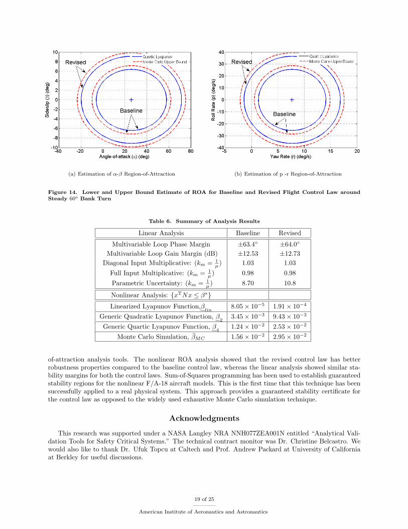
At this point, we have computed the lower and upper bounds on β∗. Figure 14 shows slices of theinner/outer approximations of the best ellipsoidal ROA approximation for both the baseline and revised

17 of 25


(a) Unstable Trajectory with IC s.t. xT0 Nx0 = 0.0295 (b) Stable Trajectory with IC s.t. xT

0 Nx0 = 0.0294

Figure 13. Time Response of F/A-18 Aircraft Revised Closed Loop Model

control laws. The blue solid lines show the slices of the inner bounds obtained from quartic Lyapunovanalysis. Every initial condition within the blue ellipses will return to the trim condition (marked as a ’+’).The red dashed lines show the slices of the outer bounds obtained from Monte Carlo analysis. There is atleast one initial condition on the outer ellipsoid which leads to a divergent trajectory. The initial conditionleading to a divergent trajectory does not necessarily lie on the slice of the ellipsoid shown in the figure.The closeness of the inner and outer ellipsoids means that we have solved, for engineering purposes, the bestROA ellipsoid problem.

Again, the aerodynamic coefficients have been fitted over a gridded α - β space of −20 ≤ β ≤ 20, and−10 ≤ α ≤ 40. Hence, the results shown in Figure 14 may not be valid over the entire region as shown inthe figure itself.

C. Summary

Table 6 summarizes the stability analysis results described in this section. There are several key points tobe gathered from this analysis. First, the F/A-18 aircraft with the baseline control law was susceptible tothe falling leaf motion. However, the linear robustness analysis did not detect any stability issues with thiscontrol law. Second, the revised control law demonstrated an ability to suppress the falling leaf motion inthe F/A-18 aircraft in flight tests. However, the linear analyses did not show a significant improvement inthe stability and robustness properties of the revised control law as compared to the baseline control law.Hence, based on the linear analyses alone both controllers should have mitigated the effect of the falling leafmotion. In contrast, the nonlinear analysis showed that the revised control law leads to a significant increasein the ROA estimate over the baseline design. This implies that the closed-loop system with the revisedcontrol law is more robust to disturbances and upset conditions. It is important to note that the region ofattraction analysis accounts for significantly nonlinearities in the aircraft dynamics. This makes the analysismore applicable to highly nonlinear flight phenomenon such as the falling leaf mode.

VI. Conclusion

In this paper, we have compared the stability and robustness properties of the two control laws (thebaseline and the revised) of the F/A-18 aircraft using linear robustness concepts and nonlinear region-

18 of 25


(a) Estimation of α-β Region-of-Attraction (b) Estimation of p -r Region-of-Attraction

Figure 14. Lower and Upper Bound Estimate of ROA for Baseline and Revised Flight Control Law aroundSteady 60o Bank Turn

Table 6. Summary of Analysis Results

Linear Analysis Baseline Revised

Multivariable Loop Phase Margin ±63.4 ±64.0

Multivariable Loop Gain Margin (dB) ±12.53 ±12.73Diagonal Input Multiplicative: (km = 1

µ ) 1.03 1.03Full Input Multiplicative: (km = 1

µ ) 0.98 0.98Parametric Uncertainty: (km = 1

µ ) 8.70 10.8

Nonlinear Analysis: xTNx ≤ β∗Linearized Lyapunov Function,β

lin8.05× 10−5 1.91× 10−4

Generic Quadratic Lyapunov Function, β2

3.45× 10−3 9.43× 10−3

Generic Quartic Lyapunov Function, β4

1.24× 10−2 2.53× 10−2

Monte Carlo Simulation, βMC 1.56× 10−2 2.95× 10−2

of-attraction analysis tools. The nonlinear ROA analysis showed that the revised control law has betterrobustness properties compared to the baseline control law, whereas the linear analysis showed similar sta-bility margins for both the control laws. Sum-of-Squares programming has been used to establish guaranteedstability regions for the nonlinear F/A-18 aircraft models. This is the first time that this technique has beensuccessfully applied to a real physical system. This approach provides a guaranteed stability certificate forthe control law as opposed to the widely used exhaustive Monte Carlo simulation technique.

Acknowledgments

This research was supported under a NASA Langley NRA NNH077ZEA001N entitled “Analytical Vali-dation Tools for Safety Critical Systems.” The technical contract monitor was Dr. Christine Belcastro. Wewould also like to thank Dr. Ufuk Topcu at Caltech and Prof. Andrew Packard at University of Californiaat Berkley for useful discussions.

19 of 25


Appendix

A. Full Model

The full six degree-of-freedom F/A-18 Hornet aircraft model is presented in this section. This model is notdirectly used for analysis presented in this paper, but is included for completeness.

1. Equations of Motion

The equations of motion described are taken from the report (chapter 4) by Napolitano and Spagnuolo.11

The state variables are:XT = [VT α β p q r φ θ ψ]

The following three equations describe the force equations of the aircraft:

VT = − qSrefm

(CD cosβ − CY sinβ) + g(cosφ cos θ sinα cosβ + sinφ cos θ sinβ

− sin θ cosα cosβ) +T

mcosα cosβ

α = − qSrefmVT cosβ

CL + q− tanβ(p cosα+ r sinα)

+g

VT cosβ(cosφ cos θ cosα+ sinα sin θ)− T sinα

mVT cosβ

β =qSrefmVT

(CY cosβ + CD sinβ) + p sinα− r cosα+g

VTcosβ sinφ cos θ

+sinβVT

(g cosα sin θ − g sinα cosφ cos θ +T

mcosα)

where q = 12ρV

2T and ρ = 0.001066 slugs

ft3 at an altitude of 25,000 ft.

The equations describing the equations of moment of the aircraft are:pqr

=

Izzκ 0 Ixz

κ

0 1Iyy

0Ixzκ 0 Ixx

κ

L

M

N

− 0 −r q

r 0 −p−q p 0

Ixx 0 −Ixz

0 Iyy 0−Ixz 0 Izz

pqr

where κ = IxxIzz − I2xz and L,M,N indicates roll, pitch, and yaw moment:LM

N

=

ClqSrefbrefCmqSref c

CnqSrefbref

The kinematic relations of the aircraft:φθ

ψ

=

1 sinφ tan θ cosφ tan θ0 cosφ − sinφ0 sinφ sec θ cosφ sec θ

p

qr

2. Full Aerodynamic Model

The aerodynamic coefficients presented here have been extracted from various papers.13–16 The aerodynamicmodel of the aircraft is presented and the coefficient values are given in Tables 7, 8.

20 of 25


Pitching Moment, Cm = Cmαα+ Cm0 + (Cmδstabα+ Cmδstab0)δstab

+c

2VT(Cmqα+ Cmq0 )q

Rolling Moment, Cl = (Clβ2α2 + Clβ1α+ Clβ0 )β + (Clδailα+ Clδail0

)δail

+ (Clδrudα+ Clδrud0)δrud +

bref2VT

(Clpα+ Clp0 )r

Yawing Moment, Cn = (Cnβ2α2 + Cnβ1α+ Cnβ0 )β + (Cnδailα+ Cnδail0

)δail

+ (Cnδrudα+ Cnδrud0)δrud + (Cnrα+ Cnr0 )

bref2VT

r

Table 7. Aerodynamic Moment Coefficients

Pitching Moment Rolling Moment Yawing MomentCmα = -0.9931 Clβ2 = 0.8102 Cnβ2 = -0.3917Cm0 = 0.1407 Clβ1 = -0.6446 Cnβ1 = 0.3648Cmδstab = 0.6401 Clβ0 = -0.0427 Cnβ0 = 0.0894Cmδstab0

= -1.1055 Clδail = -0.1553 Cnδail = -0.0213

Cmq = -14.30 Clδail0= 0.1542 Cnδail0

= 0.0051

Cmq0 = - 2.00 Clδrud = -0.0858 Cnδrud = 0.0534Clδrud0

= 0.0943 Cnδrud0= -0.0724

Clp = 0.0201 Cnr = -0.0716Clp0 = -0.3370 Cnr0 = -0.4375

Sideforce Coeffificent, CY = (CYβ2α2 + CYβ1α+ CYβ0 )β + (CYδailα+ CYδail0

)δail

+ (CYδrudα+ CYδrud0)δrud

Lift Coefficient, CL = (CLα3α3 + CLα2

α2 + CLα1α+ CLα0

) cos(2β3

)

(CLδstabα+ CLδstab0)δstab

Drag Coefficient, CD = (CDα4α4 + CDα3

α3 + CDα2α2 + CDα1

α+ CDα0) cosβ

+ CD0 + (CDδstabα+ CDδstab0)δstab

Table 8. Aerodynamic Force Coefficients

Sideforce Coefficient Drag Force Coefficient Lift Force CoefficientCYβ2 = 0.5781 CDα4

= 1.4610 CLα3= 1.1645

CYβ1 = 0.2834 CDα3= -5.7341 CLα2

= -5.4246CYβ0 = -0.8615 CDα2

= 6.3971 CLα1= 5.6770

CYδrud = -0.4486 CDα1= -0.1995 CLα0

= -0.0204CYδrud0

= 0.3079 CDα0= -1.4994 CLδstab = -0.3573

CYδail = 0.4270 CD0 = 1.5036 CLδstab0= 0.8564

CYδail0= -0.1047 CDδstab = 0.7771

CDδstab0= -0.0276

21 of 25


B. Reduced Model

1. Reduced Equations of Motion

Roll-coupled maneuvers18 of the aircraft are the focus of the analysis. The velocity, VT , is assumed to beconstant and equal to 250 ft/s.

α = − qSrefmVT

CL + q− pβ +g

VT− rβα

β =qSrefmVT

(CD + CY β) + pα− r +g

VTφ

p =1κ

(IzzL+ IxzN − [I2xz + Izz(Izz − Iyy)]rq)

q =1Iyy

(M + (Izz − Ixx)pr)

r =1κ

(IxzL+ IxxN + [I2xz + Ixx(Ixx − Iyy)]pq

φ = p

2. Reduced Aerodynamic Model

The rolling moment (Cl), pitching moment (Cm), yawing moment (Cn), and sideforce (CY ) coefficients forthe full aerodynamic model presented in Appendix A.2 are same for the reduced aerodynamic model. Thelift and drag coefficients have been approximated by employing the standard least square approximationtechnique within −20 ≤ β ≤ 20, and −10 ≤ α ≤ 40. The model is presented below:

Lift Coefficient, CL :=CLα2α2 + CLα1

α+ CLα0+ (CLδstabα+ CLδstab0

)δstabDrag Coefficient, CD:=CDα2

α2 + CDα1α+ CDβ2β

2 + (CDδstabα+ CDδstab0)δstab

Table 9. Approximated Lift & Drag Force Coefficients

Drag Coefficient Lift CoefficientCDα2

= 2.7663 CLα2= −4.5022

CDα1= 0.1140 CLα1

= 5.4854CDβ2 = 1.2838 CLα0

= −0.0406CDδstab = 0.7771 CLδstab = −0.3573CDδstab0

= −0.0275 CLδstab0= 0.8563

C. Linearized Model

The reduced order model presented in the Appendix B is used to derive the linearized model around a trimpoint. The trim values for the states and the inputs are presented in Table 3. The model xOL = AxOL+Buwith the output equation y = CxOL + Du is presented in this section. The ordering of the states, inputsand outputs are mentioned below: xT

OL = [β p r φ α q ] and u = [δail δrud δstab T ]. However, theC and D matrices will be different for each of the control law due to different feedback measurements. Theyare: yT

Baseline = [ay p r α q] and yTRevised = [ay p r α β q β]

The open loop plant, G , is represented as: G =

[A B

CRevised DRevised

]The linearized matrices for 60o

bank angle turn (Plant 4 in Table 3) is presented. The C and D matrices will be presented for the revisedflight control law. Appropriate C and D matrices for the baseline flight control law can be extracted fromthese matrices.

22 of 25


[A B

]=

−0.0059 0.4538 −1 0.1288 0.0026 0 0.0046 0.0054 0 0

−3.6680 −0.4000 0.0134 0 −0.0015 −0.1095 1.8210 0.2573 0 0

0.1382 0.0070 −0.1034 0 −0.0184 0 −0.0453 −0.1459 0 0

0 1 0 0 0 0 0 0 0 0

−0.0609 0 0 0 −0.2201 1 0 0 −0.0358 −1.755× 10−6

0 0.1305 0 0 −1.2550 −0.1984 0 0 −0.8269 0

The C and D matrices for the revised controller are as follows:

[CRevised DRevised

]=

−0.2456 0 0 0 0.02005 0 0.0356 0.0418 0 0

0 1 0 0 0 0 0 0 0 0

0 0 1 0 0 0 0 0 0 0

0 0 0 0 1 0 0 0 0 0

0 0 0 0 0 1 0 0 0 0

0 0.4538 −1 0.1288 0 0 0 0 0 0

D. Control Law State Space Realization

The state space realization of both the baseline and the revised control laws are presented here. The

controller, K =

[Ac Bc

Cc DC

]where xc = Acxc + Bcy and u = Ccxc + Dcy describes the controllers’ state

space realization with u and y as described in Appendix C.

1. Baseline Controller Realization: y = yBaseline

[Ac Bc

Cc Dc

]=

−1 0 0 4.9 0 0

0 0 0.8 0 0 0

−1 −0.5 0 −1.1 0 0

0 0 0 0 −0.8 −8

0 0 0 0 0 0

2. Revised Controller Realization: y = yRevised

[Ac Bc

Cc Dc

]=

−1 0 0 4.9 0 0 0 0

0 0 0.8 0 0 2 0 0.5

−1 −0.5 0 −1.1 0 0 0 0

0 0 0 0 −0.8 0 −8 0

0 0 0 0 0 0 0 0

23 of 25


E. Third Order Approximated Polynomial Closed-Loop Models

1. Baseline Controller Closed-Loop Model

β = 0.20127α2β − 0.0015591α2p− 0.0021718α2r + 0.0019743α2xc + 0.32034αβq + 0.065962β3

+ 0.17968αβ + 0.98314αp− 0.023426αr− 0.024926αxc + 0.134βq + 0.0025822α− 0.0068553β

+ 0.45003p + 0.1288φ− 0.99443r + 0.0056922xc

p = 17.7160α2β − 0.0277α2p− 0.0386α2r + 0.0351α2xc − 0.0033β3 + 2.1835αβ + 3.0420αp

− 0.4139αr− 0.4699αxc − 0.8151qr− 0.0015α− 3.7098β − 1.8607p− 0.1096q + 0.2799r

+ 0.2723xc

r = −1.4509α2β + 0.0105α2p + 0.0146α2r− 0.0133α2xc + 0.0012β3 − 1.0095αβ − 0.0148αp

+ 0.1410αr + 0.1854αxc − 0.7544pq− 0.0185α+ 0.1620β + 0.0455p− 0.2546r− 0.1544xc

φ = p

α = −αβr + 0.2467α2 − 0.1344αβ + 0.1473αq− βp− 0.4538βr− 0.2487α− 0.0609β + 0.7139q

q = 0.5196α2 + 4.8613αq + 0.97126pr− 1.9162α− 6.8140q + 0.1305p

xc = 4.9r− xc

2. Revised Controller Closed-Loop Model

β = 0.1831α2β − 0.0496α2p− 0.0005α2φ+ 0.0017α2r + 0.0030α2xc + 0.3203αβq + 0.0643β3

+ 0.0027αβ + 0.9557αp− 0.0054αφ+ 0.0187αr− 0.0250αxc + 0.1340βq + 0.0026α− 0.0091β

+ 0.4457p + 0.1276φ− 0.9850r + 0.0056xc

p = 1.1530α2β + 6.6577α2p− 0.0082α2φ+ 0.0308α2r− 0.1205α2xc + 18.3689β3 − 0.5080αβ

+ 2.4908αp + 0.8743αφ− 7.2037αr− 0.3495αxc − 0.8151qr− 0.0109α− 4.6009β

− 3.5186p− 0.4703φ− 0.1096q + 3.9316r + 0.2527xc

r = −1.4275α2β + 0.0546α2p + 0.0031α2φ− 0.0117α2r− 0.0132α2xc + 0.0079β3 − 1.0008αβ

− 0.0096αp− 0.0029αφ+ 0.1638αr + 0.1832αxc − 0.7544pq− 0.0182α+ 0.1854β + 0.0895p

+ 0.0124φ− 0.3509r− 0.1539xc

φ = p

α = −αβr + 0.2467α2 − 0.1344αβ + 0.1473αq− βp− 0.4538βr− 0.2487α− 0.0609β + 0.7139q

q = 0.5196α2 + 4.8613αq + 0.97126pr− 1.9162α− 6.8140q + 0.1305p

xc = 4.9r− xc

References

1Heller, M., David, R., and Holmberg, J., “Falling leaf motion suppression in the F/A-18 Hornet with revised flight controlsoftware,” AIAA Aerospace Sciences Meeting, No. AIAA-2004-542, 2004.

2Topcu, U., Packard, A., Seiler, P., and Wheeler, T., “Stability region analysis using simulations and sum-of-squaresprogramming,” Proceedings of the American Control Conference, 2007, pp. 6009–6014.

3Topcu, U., Packard, A., and Seiler, P., “Local stability analysis using simulations and sum-of-Squares programming,”Automatica, Vol. 44, No. 10, 2008, pp. 2669–2675.

4Tan, W., Nonlinear Control Analysis and Synthesis using Sum-of-Squares Programming, Ph.D. thesis, University ofCalifornia, Berkeley, 2006.

5Parrilo, P., Structured Semidefinite Programs and Semialgebraic Geometry Methods in Robustness and Optimization,Ph.D. thesis, California Institute of Technology, 2000.

6Prajna, S., Papachristodoulou, A., Seiler, P., and Parrilo, P. A., SOSTOOLS: Sum of squares optimization toolbox forMATLAB , 2004.

7Jaramillo, P. T. and Ralston, J. N., “Simulation of the F/A-18D falling leaf,” AIAA Atmospheric Flight MechanicsConference, 1996, pp. 756–766.

24 of 25


8Buttrill, S. B., Arbuckle, P. D., and Hoffler, K. D., “Simulation model of a twin-tail, high performance airplane,” Tech.Rep. NASA TM-107601, NASA, 1992.

9Stengel, R., Flight Dynamics, Princeton University Press, 2004.10Cook, M., Flight Dynamics Principles, Wiley, 1997.11Napolitano, M. R. and Spagnuolo, J. M., “Determination of the stability and control derivatives of the NASA F/A-18

HARV using flight data,” Tech. Rep. NASA CR-194838, NASA, 1993.12Stevens, B. and Lewis, F., Aircraft Control and Simulaion, John Wiley & Sons, 1992.13Napolitano, M. R., Paris, A. C., and Seanor, B. A., “Estimation of the lateral-directional aerodynamic parameters from

flight data for the NASA F/A-18 HARV,” AIAA Atmospheric Flight Mechanics Conference, No. AIAA-96-3420-CP, 1996, pp.479–489.

14Lluch, C. D., Analysis of the Out-of-Control Falling Leaf Motion using a Rotational Axis Coordinate System, Master’sthesis, Virginia Polytechnic Institue and State Unniversity, 1998.

15Napolitano, M. R., Paris, A. C., and Seanor, B. A., “Estimation of the longitudinal aerodynamic parameters from flightdata for the NASA F/A-18 HARV,” AIAA Atmospheric Flight Mechanics Conference, No. AIAA-96-3419-CP, pp. 469–478.

16Iliff, K. W. and Wang, K.-S. C., “Extraction of lateral-directional stability and control derivatives for the basic F-18aircraft at high angles of attack,” NASA TM-4786 , 1997.

17Illif, K. W. and Wang, K.-S. C., “Retrospective and recent examples of aircraft parameter identification at NASA DrydenFlight Research Center,” Journal of Aircraft , Vol. 41, No. 4, 2004.

18Schy, A. and Hannah, M. E., “Prediction of jump phenomena in roll-coupled maneuvers of airplanes,” Journal of Aircraft ,Vol. 14, No. 4, 1977, pp. 375– 382.

19Heller, M., Niewoehner, R., and Lawson, P. K., “High angle of attack control law development and testing for theF/A-18E/F Super Hornet,” AIAA Guidance, Navigation, and Control Conference, No. AIAA-1999-4051, 1999, pp. 541–551.

20Balas, G., Chiang, R., Packard, A., and Safonov, M., Robust Control Toolbox , MathWorks, 2008.21Heller, M., Niewoehner, R., and Lawson, P. K., “On the Validation of Safety Critical Aircraft Systems, Part I: An

Overview of Analytical & Simulation Methods,” AIAA Guidance, Navigation, and Control Conference, No. AIAA 2003-5559,2003.

22Khalil, H., Nonlinear Systems, Prentice Hall, 2nd ed., 1996.23Vidyasagar, M., Nonlinear Systems Analysis, Prentice Hall, 2nd ed., 1993.24Vannelli, A. and Vidyasagar, M., “Maximal Lyapunov functions and domains of attraction for autonomous nonlinear

systems,” Automatica, Vol. 21, No. 1, 1985, pp. 69–80.25Tibken, B. and Fan, Y., “Computing the domain of attraction for polynomial systems via BMI optimization methods,”

Proceedings of the American Control Conference, 2006, pp. 117–122.26Tibken, B., “Estimation of the domain of attraction for polynomial systems via LMIs,” Proceedings of the IEEE Con-

ference on Decision and Control , 2000, pp. 3860–3864.27Hauser, J. and Lai, M., “Estimating quadratic stability domains by nonsmooth optimization,” Proceedings of the Amer-

ican Control Conference, 1992, pp. 571–576.28Hachicho, O. and Tibken, B., “Estimating domains of attraction of a class of nonlinear dynamical systems with LMI

methods based on the theory of moments,” Proceedings of the IEEE Conference on Decision and Control , 2002, pp. 3150–3155.29Genesio, R., Tartaglia, M., and Vicino, A., “On the estimation of asymptotic stability regions: State of the art and new

proposals,” IEEE Transactions on Automatic Control , Vol. 30, No. 8, 1985, pp. 747–755.30Davison, E. and Kurak, E., “A computational method for determining quadratic Lyapunov functions for nonlinear

systems,” Automatica, Vol. 7, 1971, pp. 627–636.31Chiang, H.-D. and Thorp, J., “Stability regions of nonlinear dynamical systems: A constructive methodology,” IEEE

Transactions on Automatic Control , Vol. 34, No. 12, 1989, pp. 1229–1241.32Jarvis-Wloszek, Z., Lyapunov Based Analysis and Controller Synthesis for Polynomial Systems using Sum-of-Squares

Optimization, Ph.D. thesis, University of California, Berkeley, 2003.33Jarvis-Wloszek, Z., Feeley, R., Tan, W., Sun, K., and Packard, A., “Some Controls Applications of Sum of Squares

Programming,” Proceedings of the 42nd IEEE Conference on Decision and Control , Vol. 5, 2003, pp. 4676–4681.34Tan, W. and Packard, A., “Searching for control Lyapunov functions using sums of squares programming,” 42nd Annual

Allerton Conference on Communications, Control and Computing, 2004, pp. 210–219.35Jarvis-Wloszek, Z., Feeley, R., Tan, W., Sun, K., and Packard, A., Positive Polynomials in Control , Vol. 312 of Lecture

Notes in Control and Information Sciences, chap. Controls Applications of Sum of Squares Programming, Springer-Verlag,2005, pp. 3–22.

36Lofberg, J., “YALMIP : A Toolbox for Modeling and Optimization in MATLAB,” Proceedings of the CACSD Conference,Taipei, Taiwan, 2004.

37Sturm, J., “Using SeDuMi 1.02, a MATLAB toolbox for optimization over symmetric cones,” Optimization Methods andSoftware, 1999, pp. 625–653.

25 of 25


applications of linear and nonlinear robustness analysis techniques to the f/a-18 flight control

Documents