APPLICATIONS OF AUTOMATIC MESH REFINEMENT IN THE SVFLUX AND CHEMFLUX SOFTWARE PACKAGES Murray Fredlund, SoilVision Systems Ltd., Saskatoon, Saskatchewan, Canada Jason Stianson, SoilVision Systems Ltd., Saskatoon, Saskatchewan, Canada Maritz Rykaart, SRK Ltd., Vancouver, British Columbia, Canada ABSTRACT The use of finite element software packages has become commonplace in the application of geotechnical engineering. The application of the majority of this software remains hobbled by the need to manually draw finite element meshes. Manual generation of finite element meshes has further hindered the jump to the application of 3D finite element models as it remains difficult to create a 3D model in a reasonable time frame. Significant convergence problems further hinder model solution once finite element meshes are created. This paper studies the application of automatic mesh generation and automatic mesh refinement to a variety of typical problems encountered in geotechnical engineering. Common seepage, contaminant transport, and thermal geotechnical problems are examined. In particular, the application of the SVFlux and ChemFlux software packages to a variety of common problems is examined. The advantages of the automatic mesh generation and automatic mesh refinement are examined in detail. RÉSUMÉ L’utilisation des progiciels d’élément fini est devenue commune dans l’application de l’ingénierie géotechnique. L’application de la majorité de ces progiciels restes clopiner par le besoin de dessiner les mailles d’élément fini à la main. La génération manuelle des mailles d’élément fini a de plus empêché le saut de l’application des modèles à 3D car il est toujours difficile de créer un modèle à 3D dans un délai raisonnable. Les problèmes significatifs de la convergence empêchent de plus la solution du modèle dès que les mailles d’élément fini sont créées. Ce document regarde d’application de la génération de maille automatique et le raffinement de maille automatique pour une variété de problèmes typiques rencontrés en l’ingénierie géotechnique. La déperdition commune, le transport contaminé, et les problèmes géotechniques thermiques sont examinés. En particulier, l’application de SVFlux, et ChemFlux progiciels à une variété de problèmes communs est examinée. Les avantages de la génération de maille automatique et le raffinement de maille automatique sont examinés en détail. 1. INTRODUCTION The modeling of geotechnical problems such as seepage and contaminant transport has become an integral part of the practice of geotechnical engineering. The finite element and finite difference numerical methods have emerged as the primary tools used in the solution of partial differential equations describing physical processes. The finite element method, in particular, has been widely used due to its ability to offer solutions to highly irregular geometries. Commercial software packages are available in the area of geotechnical engineering. The majority of software packages require a significant time investment of the engineer in drawing the finite element mesh and achieving convergence of the model. The focus of modeling geotechnical problems should remain on the conceptual design. The details of the finite element method should be left to mathematicians. In an ideal world, mesh generation should be automatic. Mesh refinement should also be automatic based on the error encountered in the mesh. Automatic mesh generation and automatic mesh refinement is implemented in the SVFLUX and CHEMFLUX software packages. The objective of this paper is to present the advantages of automatic mesh generation and refinement when

applied to typical geotechnical engineering problems in the areas of seepage, contaminant transport, and heat flow. 2. AUTOMATIC MESH GENERATION AND

AUTOMATIC MESH REFINEMENT A general description of the automatic mesh generation and automatic mesh refinement used in the SVFLUX and CHEMFLUX software is presented below. A detailed description may be found in the user’s manuals included with the software but is omitted for the sake of brevity in this paper. The general process used in the automatic mesh generation and refinement procedure is presented in Figure 1. The process begins with an initial approximation to the mesh. The integral of the partial differential equation is then formed for each element and the relative error is estimated. The mesh is then recursively refined according to the error limit. The process continues until the relative error is less than a specified error limit. The governing partial differential equation is then solved and a Newton method of iteration is performed to bring the relative error less than a specified limit. The time-step is also iteratively refined if the problem is transient.

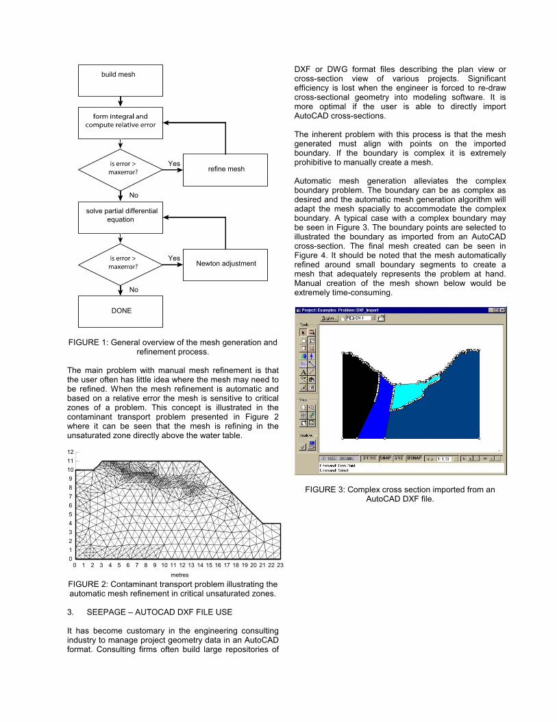
build mesh

Yes

No

refine mesh

solve partial differentialequation

Yes

No

Newton adjustment

DONE

FIGURE 1: General overview of the mesh generation and

refinement process. The main problem with manual mesh refinement is that the user often has little idea where the mesh may need to be refined. When the mesh refinement is automatic and based on a relative error the mesh is sensitive to critical zones of a problem. This concept is illustrated in the contaminant transport problem presented in Figure 2 where it can be seen that the mesh is refining in the unsaturated zone directly above the water table.

metres0 1 2 3 4 5 6 7 8 9 10 11 12 13 14 15 16 17 18 19 20 21 22 23

0123456789

101112

FIGURE 2: Contaminant transport problem illustrating the automatic mesh refinement in critical unsaturated zones.

3. SEEPAGE – AUTOCAD DXF FILE USE It has become customary in the engineering consulting industry to manage project geometry data in an AutoCAD format. Consulting firms often build large repositories of

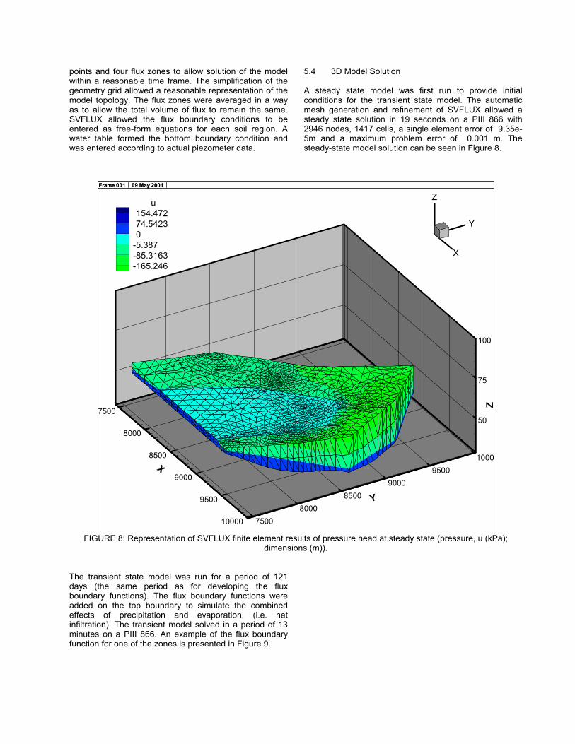
DXF or DWG format files describing the plan view or cross-section view of various projects. Significant efficiency is lost when the engineer is forced to re-draw cross-sectional geometry into modeling software. It is more optimal if the user is able to directly import AutoCAD cross-sections. The inherent problem with this process is that the mesh generated must align with points on the imported boundary. If the boundary is complex it is extremely prohibitive to manually create a mesh. Automatic mesh generation alleviates the complex boundary problem. The boundary can be as complex as desired and the automatic mesh generation algorithm will adapt the mesh spacially to accommodate the complex boundary. A typical case with a complex boundary may be seen in Figure 3. The boundary points are selected to illustrated the boundary as imported from an AutoCAD cross-section. The final mesh created can be seen in Figure 4. It should be noted that the mesh automatically refined around small boundary segments to create a mesh that adequately represents the problem at hand. Manual creation of the mesh shown below would be extremely time-consuming.

FIGURE 3: Complex cross section imported from an AutoCAD DXF file.

FIGURE 4: Mesh created by automatic mesh

generation algorithm. 4. SEEPAGE – GEOMEMBRANES

An area of seepage modeling that has been particularly challenging is the representation of geomembranes in a seepage modeling problem. The geomembrane represents a relatively thin and almost impermeable layer in typical problems. The mesh is almost impossible to create manually due to the large change in permeability over a very small spacial distance. The mesh must be altered from a relatively large element size to an extremely small element size next to the geomembrane to allow for a solution while minimizing convergence problems. Automatic mesh generation is ideal for the solution of seepage problems involving geomembranes. As the automatic mesh refinement algorithm is based on relative error of the partial differential equation the routine will automatically sense areas of high flux differentials and refine the mesh appropriately. An example of this refinement in a typical seepage problem may be seen in Figure 5.

FIGURE 5: Example of mesh refinement around a geomembrane.

5. SEEPAGE – COMPLEX 3D GEOMETRY EXAMPLE The solution of 3D finite element problems often involves creation of a highly complex, 3D mesh consisting of certain element types (i.e., tetrahedron). 3D modeling is often avoided due to the complexity of setting up the mesh. Automatic mesh generation and automatic mesh refinement are crucial for the solution of such 3D problems. An example of a real-world problem involving irregular and complex geometry is the Kidston Gold Mine. 5.1 Kidston tailings impoundment description

The gold tailings impoundment described in this article is located in Queensland, Australia. The climate is semi-arid, with an annual rainfall of 702 mm, falling mostly as high intensity showers between November and March each year. The potential evaporation of 1650 mm per year results in the annual climatic water balance to be negative. The tailings impoundment was constructed in a stream valley by means of hydraulically placed tailings behind an engineered embankment. The embankment of 5.8 km long encircles 70% of the impoundment and the overall tailings area consist of 310 ha which includes a pool of approximately 100 ha. An additional 104 ha catchment impacts on the tailings impoundment due to the impoundment being constructed against a local hill. The embankment height and subsequent tailings depth

varies between 32 m at its deepest to less than 1 m at its shallowest (Rykaart, 2001).

G

A

BC

D

E

F

Pond

Tailings

Paddy's Knob

N

S

Penstock

FIGURE 6: Simplified plan view of the Kidston tailings

impoundment, showing the penstock location after 1991, and the piezometer section lines.

Both a saturated and an unsaturated zone exist in the tailings impoundment due to the presence of the pool. The established phreatic surface has a shape that is governed by the tailings properties, and the exit location is determined by the presence of drains in the embankment walls. Let us consider a typical cross-section at any location through the tailings impoundment (Figure 7(a)) there would be an unsaturated zone of tailings which varies in thickness from the embankment end to the pool end. The top tailings impoundment surface (beach profile) along this typical cross-section would be subject to all the usual water balance components of precipitation (P), evapotranspiration (ET), infiltration (I), runoff (R), recharge (Re), and seepage (S). It would however be expected that there would be a spatial variation in the magnitude of these components as one move between the embankment and the pool. The reason for this is the availability of moisture in the profile, which is governed by the presence of the phreatic level (Staley, 1957). Therefore, at a point close to the embankment, the anticipated evaporation would be a minimum, and as one moves towards the pool the evaporation should increase until it reaches a maximum (potential evaporation) at the pool edge. Similarly, it is anticipated that the infiltration would be a maximum close to the embankment, decreasing towards the pool. This is illustrated by the graph in Figure 7(b).

Evaporation InfiltrationMin Min

MaxMax

P

R

RePool

Saturated tailings

Embank-ment

ET

S

IUnsaturated tailings

(a)

(b)

FIGURE 7: (a) Typical cross-section through a tailings

impoundment, (b) Spatial distribution of surface fluxes of infiltration and evaporation.

5.2 3D Seepage Modeling In order to prove that the spatial flux boundary functions presented in Figure 2 are in fact a reasonable approximation of the actual surface flux boundary conditions, it had to be used as an input in multidimensional seepage analysis models, and the seepage rates from the drains of the tailings impoundment had to be predicted. If the seepage rates were in fact a good match, the flux boundary functions could be considered to have fulfilled their function. Modeling of seepage in the tailings impoundment presented a unique challenge. Firstly, the complexity of the model dictated that a 3D seepage model be used. A 2-D cross-section of the tailings impoundment would not capture the essence of the problem nor would it yield representative flow rates. The actual 3D modeling of the flow regime through the tailings impoundment presented a significant challenge in itself. The model requirements included complex, irregular geometry, unsaturated flow, irregular flux sections, and highly complex boundary conditions. For practical purposes the development of the 3D model was also required to be able to be done within a reasonable time period. The SVFLUX (SoilVision Systems, 2001) model developed by SoilVision Systems Ltd. was selected based on its ability to model complex, highly irregular 3D problems with a relatively short learning curve. 5.3 3D Model Soil Properties and Boundary

Conditions The selected material properties were identical to those used in developing the surface flux boundary functions described in earlier sections of this article, resulting in the use of three soil-water characteristic curves and a saturated surface hydraulic conductivity function. Detailed survey data was available for the base and surface topography of the problem and would have to be used to describe the model. The survey data resulted in a grid of 2000 points. Furthermore, 13 zones had been isolated containing flux boundary conditions. However, the detailed data was simplified to a geometry grid of 120

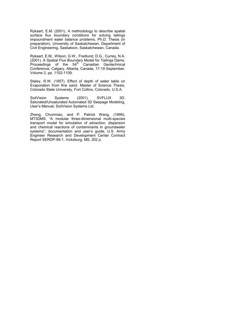
points and four flux zones to allow solution of the model within a reasonable time frame. The simplification of the geometry grid allowed a reasonable representation of the model topology. The flux zones were averaged in a way as to allow the total volume of flux to remain the same. SVFLUX allowed the flux boundary conditions to be entered as free-form equations for each soil region. A water table formed the bottom boundary condition and was entered according to actual piezometer data.

5.4 3D Model Solution A steady state model was first run to provide initial conditions for the transient state model. The automatic mesh generation and refinement of SVFLUX allowed a steady state solution in 19 seconds on a PIII 866 with 2946 nodes, 1417 cells, a single element error of 9.35e-5m and a maximum problem error of 0.001 m. The steady-state model solution can be seen in Figure 8.

50

75

100

Z

7500

8000

8500

9000

9500

10000

X

75008000

85009000

95001000

Y

X

Y

Zu154.47274.54230

-5.387-85.3163-165.246

Frame 001 09 May 2001 Frame 001 09 May 2001

FIGURE 8: Representation of SVFLUX finite element results of pressure head at steady state (pressure, u (kPa);

dimensions (m)). The transient state model was run for a period of 121 days (the same period as for developing the flux boundary functions). The flux boundary functions were added on the top boundary to simulate the combined effects of precipitation and evaporation, (i.e. net infiltration). The transient model solved in a period of 13 minutes on a PIII 866. An example of the flux boundary function for one of the zones is presented in Figure 9.

Mar

Feb

Jan

Dec

-3.0

-2.5

-2.0

-1.5

-1.0

-0.5

0.0

0.5N

et in

filtra

tion

flux

(mm

/day

)

FIGURE 9: Typical flux boundary function for one of the zones, presenting monthly distribution of net infiltration.

The combined flux boundary functions caused a net loss of water from the system over the four-month period. Flow upward through the unsaturated zone is significant, as the net flow is negative. The negative flux boundary was countered by the water source of the pond at the center of the tailings (the level of which was varied according to a function describing actual measured pond levels). Seven seepage flux surfaces were placed in the 3D model to monitor seepage outflow from the tailings impoundment. A total volume of water exited the problem over a period of four months with an average flow rate of 7.6 L/s. Actual seepage flow rates from the tailings impoundment measured over the 4 months suggests an average seepage rate of 10.8 L/s (Rykaart, 2001). Considering the inaccuracies involved in the actual seepage measurements, which includes an estimated 15% overestimation due to surface runoff intercepted in the seepage drains, combined with the complexity of the problem as a whole, the flux boundary function seems to provide an excellent solution for the problem. 5.5 Summary of 3D Example The use of a flux boundary function to describe and predict the surface flux boundary conditions through the top unsaturated tailings cross-section in itself is a great benefit for the tailings engineer. The combined advantage of using this function as a direct input, into 3D seepage modeling software to assist in long-term water balance calculations makes it a worthwhile effort altogether. Another great benefit illustrated in this study is the way the 3D model could be simplified using the same boundary conditions and material properties used in developing the flux boundary function, effectively eliminating the guesswork normally associated with setting up complex 3D problems. This could all be done without sacrificing accuracy. Finally, no 3D modeling is ever easy, and the tool used invariably affects the reliability of the results. The authors used SVFLUX due to its relatively short learning curve, and found it to be highly effective, as an engineering tool. 6. CONTAMINANT TRANSPORT – ADVECTION

ONLY

For advection-dominated problems, the solution of the contaminant transport partial differential equation is complicated by having to solve two numerical problems. The first problem is numerical dispersion. Numerical dispersion is similar to physical dispersion but is caused by truncation error. The second type of problem is artificial oscillation. Artificial oscillation tends to become more pronounced as the concentration front becomes sharper. The two numerical problems are illustrated in Figure 10. A set of one-dimensional benchmark problems used to test the ability of CHEMFLUX against the MT3DMS solver. The benchmark problems were originally published in the MT3DMS User’s Manual (Zheng and Wang , 1999). Comparison to the MT3DMS solver was performed because of the widespread use of the solver and because of the rigorous methods implemented in the solver to alleviate the numerical problems. The MT3DMS code implements three mathematical methods to obtain accurate results to transport problems dominated by one of the above processes. The mathematical methods include method of characteristics (MOC), modified method of characteristics (MMOC), and total-variation-diminishing (TVD) method. CHEMFLUX will be tested against the MT3DMS code to illustrate its ability to use one mathematical method, the finite element (FEM) method, to give accurate results to any transport problem regardless of the dominating process. 6.1 Problem Description

6.1.1 Soil Properties Groundwater seepage velocity (ν) = 0.24 m/day Porosity (θ) = 0.25 Simulation time (t) = 2,000 days Case 1a: α = 0, R = 0, λ = 0

Advection only Case 1b: α = 10m, R = 0, λ = 0

Advection and dispersion Case 1c: α = 10m, R = 5, λ = 0

Advection, dispersion, and adsorption Case 1d: α = 10m, R = 5, λ = 0.002d-1

Advection, dispersion, adsorption, and decay

6.1.2 Geometry/Boundary Conditions

1000m

1m c = 1 c = 0gradc = 0

gradc = 0

The problem is a simple rectangle that is 1000m long and 1m high. The seepage solution was prepared in SVFLUX. Arbitrary constant head boundary conditions were chosen in SVFLUX to obtain the required groundwater seepage velocity. The CHEMFLUX model uses both the Dirichlet boundary condition and the

Neuman boundary condition. The Dirichlet boundary condition specifies a concentration along a boundary for the duration of the solution, while the Neuman boundary condition specifies a concentration gradient. A concentration of 1g/m3 is specified along the left boundary; a concentration of 0g/m3 is specified along the right boundary, while a concentration gradient of zero is specified for the top and bottom boundaries of the rectangle. The solution results may be seen in Figure 10.

6.1.3 Results

0

0.2

0.4

0.6

0.8

1

1.2

0 100 200 300 400 500 600 700 800 900 1000

Distance (m)

C/C

o

CHEMFLUX Case1a FEMCHEMFLUX Case1b FEMCHEMFLUX Case1c FEMCHEMFLUX Case1d FEMMT3D Case1a TVDMT3D Case1b MOCMT3D Case1c MMOCMT3D Case1d MMOCMT3D Case1a Upstream FD

FIGURE 10: CHEMFLUX vs MT3DMS

• Case 1a: Case 1a is pure advection. CHEMFLUX is compared to the MT3DMS total-variation-diminishing (TVD) method. It should be noted that the method of characteristics (MOC) implemented in the MT3DMS model is free of numerical dispersion. However, the MOC technique can also lead to large mass balance discrepancies under certain situations because the discrete nature of the particle-tracking-based mixed Eulerian-Lagrangian solution techniques does not guarantee local mass conservation at a particular time-step (Zheng and Wang, 1999). Therefore, CHEMFLUX is compared to the third-order TVD method available in MT3DMS. This third-order ULTIMATE scheme is mass conservative, without excessive numerical dispersion, and essentially oscillation-free (Zheng and Wang, 1999). The ULTIMATE scheme was significantly superior to some popular second-order TVD schemes (Leonard, 1988) and was considered to be possibly the most accurate practical method available (Roache, 1992). For advection-dominated problems that exist under many field conditions, an Eulerian method may be susceptible to excessive numerical dispersion or artificial oscillation. To overcome these problems, restrictively small grid spacing and time-steps may be required (Zheng and Wang, 1999). CHEMFLUX utilizes both automatic mesh refinement and automatic time step refinement giving CHEMFLUX the power to overcome artificial oscillation and numerical dispersion. The above results show that CHEMFLUX is comparably as accurate as the TVD

scheme and far surpasses the results of the upstream finite difference scheme. • Case 1b: Case 1b models the affects of advection and dispersion. In this case the front is no longer abrupt due to the inclusion of dispersion. For this case CHEMFLUX is compared to the MOC scheme, as the results from the TVD scheme were not available. The CHEMFLUX software matches the solution of the MOC scheme and provides added assurance that the solution is mass conservative. • Case 1c: Case 1c models the affect of advection, dispersion, and adsorption. In this case the front does not move as far as the pure advection case or the advection dispersion case due to chemical adsorbing to soil particles. CHEMFLUX is compared to the modified method of characteristics (MMOC). This method is used only when the problem will is not dominated by advection. The MMOC technique introduces considerable numerical dispersion, especially for sharp front problems (Zheng and Wang, 1999). The MMOC technique is normally faster than the MOC technique, requires much less memory, and is also free of artificial oscillations. CHEMFLUX results are just as reliable as those obtained with the MMOC while providing benefits over the MOC in model description time savings, memory requirements, and lack of numerical oscillation.

• Case 1d: Case 1d models the affect of advection, dispersion, adsorption, and decay. This case illustrates the affect decay has on the transport process causing the front to move even slower across the problem. CHEMFLUX is again compared against the MMOC and it again provides comparible results. 7. SUMMARY Automatic mesh refinement dramatically improves the ability of the geotechnical engineer to rapidly model geotechnical engineering problems. Mesh refinement is based on relative error and is therefore superior to manual mesh generation techniques. Complex problems involving geomembranes are readily solvable. Model design time is further improved by the ability to import cross-sections directly from AutoCAD drawings. Complex 3D models are now possible in reasonable time frames. Contaminant transport problems may also be accurately solved with the irregular geometry advantages of the finite element method. All of these examples result in a new level of powerful software that allows the consulting geotechnical engineer to dramatically improve the application of numerical models. 8. REFERENCES

Rykaart, E.M. (2001). A methodology to describe spatial surface flux boundary conditions for solving tailings impoundment water balance problems. Ph.D. Thesis (in preparation), University of Saskatchewan, Department of Civil Engineering, Saskatoon, Saskatchewan, Canada. Rykaart, E.M., Wilson, G.W., Fredlund, D.G., Currey, N.A. (2001). A Spatial Flux Boundary Model for Tailings Dams. Proceedings of the 54th Canadian Geotechnical Conference, Calgary, Alberta, Canada, 17-19 September. Volume 2, pp. 1102-1109. Staley, R.W. (1957). Effect of depth of water table on Evaporation from fine sand. Master of Science Thesis, Colorado State University, Fort Collins, Colorado, U.S.A. SoilVision Systems (2001). SVFLUX 3D: Saturated/Unsaturated Automated 3D Seepage Modeling, User’s Manual, SoilVision Systems Ltd. Zheng, Chunmiao, and P. Patrick Wang, (1999), MT3DMS, “A modular three-dimensional multi-species transport model for simulation of advection, dispersion and chemical reactions of contaminants in groundwater systems”; documentation and user’s guide, U.S. Army Engineer Research and Development Center Contract Report SERDP-99-1, Vicksburg, MS, 202 p.