application specific instruction set processor design nikolaos kavvadias april 2003 (converted...

Application Specific Instruction set Processor Design

Nikolaos Kavvadias

April 2003 (converted to .odp: 2010/11/25)

Electronics and Computers Div.,

Department of Physics,

Aristotle University of Thessaloniki,

54124, Thessaloniki, Greece

E-mail: [email protected]

• Challenges in ASIP design

• Introduction to the ASIP design flow

• A methodology for synthesis of Application Specific Instruction Sets

• Architecture design space exploration for ASIPs

• Case study: ASIP design for an image compositing application

Outline

Outline

• Challenges in ASIP designChallenges in ASIP design


• A methodology for joint design of instruction sets and micro-architectures



Main challenges in embedded systems design

• Embedded systems form a market that is growing more rapidly than that of general purpose computers

• Embedded processors are extensively used in digital wireless communications and multimedia consumer electronics (e.g. cellular phones, video cameras, audio players, video-game consoles)

• These complex systems relay on power hungry algorithms

• The portability of these systems makes energy consumption a particularly critical design concern with performance and cost

• At the same time, levels of microelectronic integration continue to rise enabling more integrated functionality on a single chip

Main challenges in embedded systems design (2)

• Basic challenge:

How to effectively design first-time-right complex systems-on-a-chip that meet multiple stringent design constraints?

• To do that it is important to maximize the flexibility/programmability of the target system architecture moving as much functionality as possible to embedded software

• General purpose embedded processors may not be able to deliver the performance required by the application and they may be prohibitively expensive/inefficient, e.g. to energy consumption

• Thus, the embedded systems industry has shown an increasing interest in Application-Specific-Set Processors (ASIPs)

• Processors designed for a particular application or set of applications

• An ASIP is designed to exploit special characteristics in the target application in order to meet performance, cost and energy requirements

• By spending silicon where it truly matters, these processors are smaller and simpler than their general-purpose counterparts, able to run at higher clock frequencies and more energy efficient

• Obtaining best results requires proper decisions at the joint instruction set and micro-architectural level

• Considered as a balance between two extremes: ASICs and general-purpose processors

What are ASIPs

Potential benefits from adopting an ASIP solution

• Benefits of an ASIP solution:

Maintain a level of flexibility/programmability through an instruction set

Overcome the problems of conventional RISC/DSP architectures:

a. Fixed level of parallelism which may prove inefficient for real-time applications of high computational complexity

b. Prohibitively high energy consumption

c. Time-critical tasks that require the incorporation of dedicated hardware modules

Shortening of debugging/verification time. Key enabler is FPGA technology (rapid prototyping/reconfigurable platforms)

Challenges in ASIP design

• Given an application or set of applications, the design of an instruction set and micro-architecture to meet the design constraints of area, performance and energy consumption requires:

Definition of the design space of both instruction sets and micro-architectures to be explored

Understanding of the relationships between application characteristics and design (mapping of application on hardware)

Development of tools (assembler/linker, compiler backend and frontend, simulator, debugger) for efficient design space exploration

Outline


• Introduction to the ASIP design flowIntroduction to the ASIP design flow




Issues in application-specific processor design

• Instruction Set Synthesis (ISS) Generates an instruction set that optimizes an objective function (instruction set size, cycle count, cycle time, gate count)

• Instruction Set Mapping (ISM) or Code Generation (CG)

Systematic mapping of the application into assembly code with the given instruction set

• Microarchitecture Synthesis (MS) Given an instruction set specification, this approach synthesizes a micro-architecture at the RTL, which implements the instruction set

Steps in ASIP Synthesis

• Main steps in a typical methodology for ASIP synthesis:

1. Application analysis

2. Architectural design space exploration

3. Instruction set generation

4. Code synthesis

5. Hardware synthesis

Flow Diagram of a typical ASIP Design Methodology

Application &Design Constraints

Application Analysis

Architectural Design Space Exploration

Instruction SetGeneration

Code Synthesis Hardware Synthesis

Object Code Processor Description

Application analysis

• Input in the ASIP design process is an application or a set of applications

• The target application(s) along with its test data and design constraints are analyzed either statically (profilers) or dynamically

• Major task is to extract coarse-level requirements (micro-operations) which will lead the instruction set and micro-architecture design procedure

• Dynamic profiling: The original application description, in a high-level language is instrumented with performance counters and the modified application code is executed

Application analysis (2)

• Application analysis output may includes:

number of operations and functions

frequency of individual instructions and sequence of contiguous instructions

average basic block sizes

data types and their access methods

ratio of address computation instructions to data computation instructions

ratio of input/output instructions to total instructions

• It serves as a guide for the subsequent steps in ASIP synthesis

Architectural Exploration

• It is important to deside about a processor architecture suitable for target application

• Determination of a set of architecture candidates for a specific application(s) given the design constraints

• Performance, hardware cost and power consumption estimation and selection of the optimum one

• Performance estimation can be based on scheduling or simulation

Architectural Exploration (2)

• Block diagram for a typical architecture explorer

inpu t from app lica tionana lys is

perfo rm anceestim ator fo r a

spec ificarch itecture

searchcontro l

a rch itecture des ignspace

se lectedarch itecture (s)

• The selection process typically can be viewed to consist of a search technique over the design space driven by a performance estimator

Architecture design space

• Need for a good parameterized model of the architecture

• Different values should can be assigned to the parameters while keeping design constraints into consideration

• The size of the design space is defined by the number of parameters and the range of values which can be assigned to these paramters

Architecture design space (2)

• Parameters of architecture models:

- number of functional units of different types

- storage elements

- interconnect resources

- pipelining

- number of pipeline stages

- instruction level parallelism

- addressing support

- memory hierarchy

- instruction packing

- latency of functional units and operations

• All parameters together support a large design space

Scheduling-based performance estimation

ArchitectureDescription Application

Profiler

Retargetable Estimator

Performance andother Estimates

• The problem is formulated as resource constrained scheduling problem with the selected architectural components as the resources and the application is scheduled to generate an estimate of the cycle count

Simulation-based performance estimation

Application(HLL)

ArchitectureDescription

Trace Data

RetargetableCompiler

SimulatorObjectCode

• The application is mapped on a simulation model of the architecture for performance estimation

• A simulation model of the architecture is generated and the application is simulated to compute the performance

• The application is translated into an intermediate code composed of simple instructions directly expressing primitive hardware functionalities

• A sequential code simulation is performed to validate the code and to extract early features which can perform preliminary architectural choices

• The simulator reports performance energy consumption and statistics about resource utilization

• Optimization techniques are applied to increase the degree of parallelism

• Frequently executed sequence of instructions can be subistuted by the introduction of new instructions

Simulation-based performance estimation (2)

Instruction set generation (synthesis)

• Instruction set is synthesized for a particular application based on the application requirements, quantified in terms of the required micro-operations and their frequencies

• A methodology for instruction set synthesis should utilize: A model for the micro-architecture An objective function that establishes a metric for the fitness of the solution (both instruction set and micro-architecture) Design (hardware resource and timing) constraints are considered

• In the approach to be discussed [Huang95] instruction set design is shown as a modified scheduling problem of the application micro-operations. At the same step, instruction set and application code is generated

Code Synthesis: Retargetable code generator

• Retargetable code generator: The architecture template and instruction set architecture and application are accepted as inputs, in order to generate object code

Application (HLL)

Architecturetemplate

Instruction setArchitecture (ISA)

Retargetable code generator

Object code

Code Synthesis: Compiler generator

• Compiler generator (or Compiler – Compiler): Accept architecture template and instruction set as inputs and generate a customized compiler which accepts the application programs

Application (HLL)



Retargetable compiler generator

Object code

Customized compiler

Hardware synthesis

• Hardware synthesis refers to the generation of the HDL descriptions for the processor modules

• Automatic generation of RTL descriptions, for both simulation (and functional verification) and logic synthesis purposes

Design constraints



Automatic hardware generation

VHDL descriptionof the processor

Outline



• A methodology for synthesis of Application Specific Instruction SetsA methodology for synthesis of Application Specific Instruction Sets



• The performance of a microprocessor-based system depends on how efficiently the application is mapped to the hardware

• Key issue determining the success of the mapping is the design of the instruction set

•A jointly design of the instruction set and microarchitecture is required

• Here the following ASIP design methodology is presented:

I.J. Huang and A.M. Despain, “Synthesis of Application Specific Instruction Sets,” IEEE Transacions on Computer Aided Design, vol 14, June 1995

Key issue in designing efficient ASIPs

• The design problem is formulated as a modified scheduling problem

• The application is represented by micro-operations

• The micro-operations are scheduled on a parameterized pipelined micro-architecture folowing the design constraints

• Instructions are formed by an instruction formation process which is integrated into the scheduling process

• The compiled code of the application is generated using the synthesized instruction set

• A simulation annealing scheme is used to solve for the schedule and the instruction set

Presented ASIP design methodology

Models for instruction sets

• An instruction contains one or more parallel micro-operations (MOPs)

• MOPs are controlled via instruction fields belonging to some field types

• The instruction word length is defined by the designer (e.g. 32 bits)

• Example of instruction field types and corresponding bit-widths

• Examples of instruction formats

Instruction formats

• Example 1: The ADD instruction

Instruction description: add(R1,R2,immed)

Corresponding MOP: R1 <- R2 + immed

• Example 2: INC instruction

Instruction description: inc(R)

Corresponding MOP: R <- R + 1 (21 bits unused in the format)

Operand encoding

• The operands of instructions can be encoded to become part of the opcode in two ways:

1. A specific value can be permanently assigned to an operand and becomes implicit to the opcode (eg. Immed=1)

2. Unifying the register specifiers (eg. R1=R2)

• Encoding operands saves instruction field, at the cost of possibly larger instruction set size, additional connections and hardwired constants in the datapath

Operand encoding (2)

• Encoding allows more MOPs to be packed into a single instruction

• Example: if it happens very often that the values of two independent

registers are increased by one at the same time, a new instruction can be considered

Incd(R1,R2) => ‘R1<-R1+1; R2<-R2+1’ using only 16 bits

while the generalized form ‘R1<-R2+Immed1; R3<-R4+Immed2’

uses 58 bits violating the design constraints (32 bits)

Basic pipeline micro-architecture model

• Processor operation can be functionally partitioned into 6 pipeline stages

• Variations to the basic pipeline structure:

1. IF-ID/R-A-M-W: 5-stage MIPS-like pipeline, single format for registers

2. IF-ID-R-A/M-W: 5-stage pipeline, no displacement addressing

Pipeline micro-architecture details• The pipeline is controlled in a data-stationary fashion

• Data-stationary control: the opcode flows through the pipeline in synchronization with the data being processed in the data path

• Pipeline stage controllers: At each stage, the opcode together with the possible status bits from the data path, is decoded to generate the control signals necessary to drive the data path.

Pipeline micro-architecture details (2)

• This RISC-style pipeline supports single-cycle instructions

• Multiple-cycle instructions can be accommodated if execution can be stalled to wait for multi-cycle functional units to complete

• More generally, multiple-cycle arithmetic/logic operations, memory access, and change of control flow (branch/jump/call) are supported by specifying the delay cycles as design parameters

The specification for the target micro-architecture

• The target micro-architecture can be fully described by specifying the supported MOPs and a set of parameters

• The supported MOPs describe the functionality supported by the micro-architecture, and the connectivity among modules in the data path

The specification for the target micro-architecture (2)

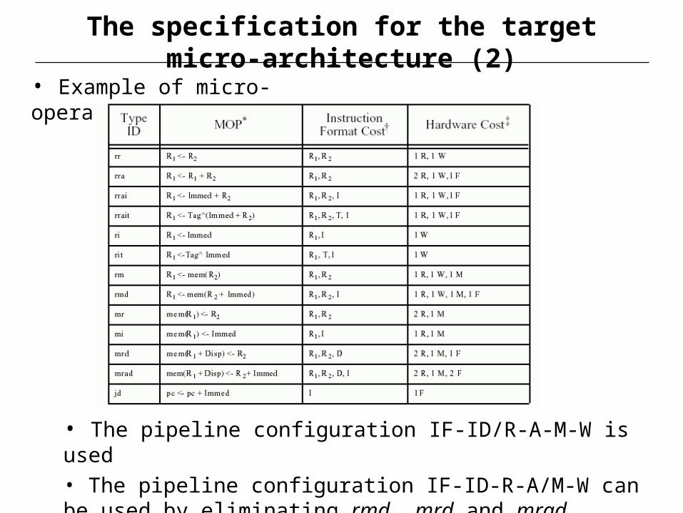
• Example of micro-operations

• The pipeline configuration IF-ID/R-A-M-W is used

• The pipeline configuration IF-ID-R-A/M-W can be used by eliminating rmd, mrd and mrad

Micro-architecture parameters

• The set of parameters describes resource allocation and timing

• Examples of parameters:

number of register file read/write ports (R/W)

number of memory ports (M)

number of functional units (F)

size of register file and memory

latencies of operations (multi-cycle functional units)

delay cycles between operations (registering/bypassing outputs)

Micro-architecture parameters (2)

• Example of resource size and latency parameters

• Example of delay cycle parameters (can model bypassing buses)

Instruction format and hardware costs

• Each MOP supported by the data path is assigned costs for the instruction format and hardware resources

• Instruction format costs:

instruction fields, including register index, function selectors and immediate data

• Hardware costs:

hardware resources as read/write ports of the register file, memory ports, and function units

Models for application benchmarks

• Each application benchmark is represented as a group of basic blocks

• Basic block: sequential code between consecutive control flow boundaries

• Basic block weights are determined dynamically by profiling, and is usually used to indicate how many times the basic block is executed in the benchmark

• An initial specification for the required MOPs is defined

• The basic blocks are mapped to control/data flow graphs (CDFGs) of MOPs based on the given MOP specification

• Different micro-architectures result in different MOP specifications, which may map the basic blocks to different CDFGs

Basic block representation

• Example: CDFG for the MOPs of simple basic block

Control dependencies are represented by dashed arrows

Data-related dependencies are represented by solid arrows

Synthesis of Instruction set

• The instruction set design problem can be formulated as a modified scheduling problem

Application(CDFGs)

μ-Arch. SpecsDesign constraintsObjective function

Compiled codeInstruction set

SchedulingInstructionFormation

• The MOPs in the CDFG are scheduled into time steps, subject to various constraints

• While scheduling MOPs into time steps, instructions are formed at the same time

Examples of micro-operation schedules

• Example schedule 1 for the simple basic block:

This is a serialized schedule with 1 MOP per time step

One-cycle delay for the jump MOP and zero cycle delay for the MOPs are assumed

Examples of micro-operation schedules (2)

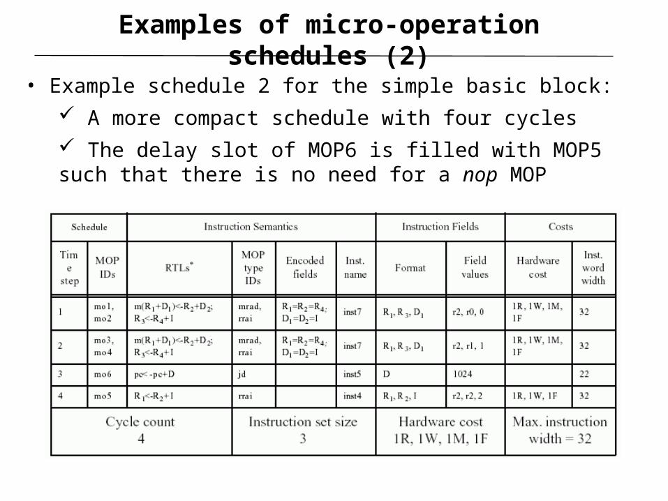
• Example schedule 2 for the simple basic block:

A more compact schedule with four cycles

The delay slot of MOP6 is filled with MOP5 such that there is no need for a nop MOP

Instruction formation details

• The semantics of an instruction can be represented by a binary tuple <MOPTypeIDs, IMPFields>, where MOPTypeIDs is a list of type IDs of MOPs contained in the instruction and IMPFields is a list of fields that are encoded into the opcode

• Example 1: add(R1, R2, immed) is represented by <[rrai], []>The MOP type ID contains MOP: R1 <- R2 + immed No fields are encoded (second argument of the tuple is empty)

• Example 2: inc(R) is represented by <[rrai],[R1=R2, immed=1]> inc instruction is an encoded version of the add (same MOPType ID) R1=R2 unifies the corresponding register specifiers, and immed=1 assigns the immediate operand a fixed value

• Instructions are generated from time steps in the schedule, with each time step corresponding to one instruction

Code generation resulting from the scheduling/instruction formation process

• The compiled code can be obtained easily from the instruction names and instantiated field values

• Example: Compiled code from the scheduled basic block of second Table

inst7(r2, r0, 0)inst7(r2, r1, 1)inst5(1024)inst4(r2, r2, 2)

• The instruction set is formed by taking the union of instructions generated from all time steps eg. inst4, instr5, instr7

Performance (cycle count) and Costs

• Execution cycles is determined as the weighted sum of the lengths (number of time steps) of the scheduled basic blocks in the benchmark

• The length of the basic cost includes nop slots which are inserted by the design process to preserve the constraints due to multi-cycle operations

• The design process will try to eliminate the nop slots by reordering other independent operations into the nop slots

• Each instruction has two costs associated with it

The total number of bits required to represent the instruction

Hardware costs (the collection of the resources required by all MOPs contained in the instruction, minus the shared resources

• The global hardware resources are obtained by choosing the maximal number for each resource type from all instructions

Increase the efficiency of the instruction set

• Compact and powerful instructions can be synthesized by:

packing more MOPs into a single instruction

making fields implicit

making register ports unified to satisfy the cost constraints

• This is particularly useful in an application specific environment where instruction sets can be customized to produce compact and efficient codes for the intended applications

Types of constraints

• The MOPs are scheduled into times steps while data/control dependencies and timing constraints (for multi-cycle MOPs) have to be satisfied

• Data dependent MOPs have to be scheduled into different time steps, subject to the precedent relationship and timing constraints (except single cycle MOPs with Write-after-Read dependencies)

• In case of control dependency with a timing constraint, e.g. a delayed jump The MOPs that are data-independent to the jump/branch MOPs can be scheduled into the time step before the jump/branch MOPs or the delay slots after the jump/branch MOPs The length of the delay slots is determined by the timing constraint

• Other constraints: instruction word width, hardware resources consumed by the instructions, the size of the instruction set that the opcode field can afford

Objective function

• An objective function is necessary to control the performance/cost trade-off

• The goal of the design system is to minimize a given object function

• The objective function has to account for parameters as:

cycle count C (as determined by the performance metrics)

instruction set size S (represents the cost metrics)

improvement in performance compared to other candidates, P

Objective = (100/P) • ln(C) + S

• The design constraints are either captured by the objective function (not in this case) or examined separately

Simulated annealing algorithm

• The instruction set design problem is formulated as a scheduling problem

• The scheduling problem is solved by a simulation annealing scheme

An initial design state consisting of an initial schedule and its derived instruction set (generated by a preprocessor) is given to the design system

then a simulated annealing process is invoked to modify the design state in order to optimize the objective function

The simulated annealing process is run until the design state achieves an equilibrium state

The basic simulated annealing algorithm

• At each temperature (outer while loop), several movements (changes of the design state) are generated by the inner while loop. The number of movements is specified by the designer

Move operators

• Move operators are applied to change the design state

• They provide methods of manipulating the MOPs and time steps

• Move operators can be classified into three groups

Manipulation of the instruction semantics and Format of a selected time step

Manipulation of MOPs locations

Micro-architecture-dependent operators (include methods that explore the special properties of the target micro-architectures)

Manipulation of the instruction semantics and format

• Unification: Unify two register accesses in the MOPs (e.g. R1=R2 in inc(R)). Decreases the instruction word width and register read/write ports

• Split: Cancel the effect of the unification operator. Increases the instruction word width and register read/write ports

• Implicit value: Bind a register specifier to a specific register, or an immediate data field to a specific value (as immed=1 in the inc). Decreases the instruction word width

• Explicit value: Cancel the effect of the “implicit value” operator. Increase in the instruction word width

• Generalization: Encoded operands in an instruction format are made general (explicit in the instruction fields). Increased instruction word width and hardware resources

Manipulation of MOP’s locations

• These move operators are subject to the data/control dependencies and delay constraints when moving MOPs

• Interchange: Interchange the locations of two MOPs from different time steps. Changes the semantics and formats of the two instructions in the corresponding time steps

• Displacement: Displaces a MOP to another time step. Simplifies the instruction in the original time step and enriches the instruction in the destination time step

• Insertion: Insert an empty time step after or before the selected time step and move one MOP to the new time slot. Increases the cycle count

• Deletion: Delete the selected time step if it is an empty one. Decreases the cycle count

• The move operators may change the resource usage in the selected time steps.

Micro-architecture dependent operators

• These move operators explore the special properties of the target micro-architectures

• Example: Tradeoffs in functional unit interconnections

- The target micro-architecture provides two data routing possibilities:

1. register file functional unit register file

2. register file register file

- Then, the following MOPs are equivalent:

1. rrai: R1 R2 + Immed (Immed=0)

2. rr: R1 R2

- These have different costs in hardware and instruction format and can be transformed from one to another

Example: Changing the design state with move operators

• In the following tables, a sequence of operators are applied to transform the schedule (one design state) to a better design state

1) Displacement: displace the MO2 from time step 2 to 1

Example: Changing the design state with move operators (2)

2) Unification: unify fields D1 and D2 in time step 1

3) Unification: unify fields D1 and I in time step 1

4) Unification: unify fields R1 and R2 in time step 1

5) Unification: unify fields R1 and R4 in time step 1


6) Deletion: delete the empty time step 2

7) Displacement: displace the MO4 from time step 4 to 3



9) Unification: unify fields D1 and I in time step 3

10) Unification: unify fields R1 and R4 in the time step 3

11) Displacement: displace the MO5 from time step 5 to 7 (see table above)


Heuristics for target selection

• During each iteration, the design space is examined whether it violates the design constraints

• In case of constraint violation a time step is randomly selected from a pool of time steps that violate design constraints

• If more than one constraint are violated, the hardware resource violations get higher priority than instruction word width violations

• Instruction word width violations: one of the following move operators is applied randomly: “unification”, “implicit value”, “interchange”, “displacement”, “insertion”

• Resource violations: one of the following move operators is applied randomly: “unification” (register port constraint), “implicit value”, “displacement”, or “insertion”

Selection weights

• In case of no constraints, all move operations are eligible for changing the design state

• A basic block is selected with the probability Selectioni which is the selection weight of the basic block i

Fi: execution frequency of the basic block

Ni: number of MOPs in the basic block

iii

iii NF

NFSelection

• The selection weight is intended to denote the degree of importance of a basic block in the benchmark

Temperature and Cooling schedule

• The cooling schedule is controlled by five parameters

1) Initial temperature (T0). It should be high enough so that there is no rejection for high-cost states at the initial temperature

2) The number of movements (M) tried at each temperature. These are proportional to the total number of MOPs in the benchmarks.

3) The next temperature (T) of the current temperature (e.g. 90%)

4) Low and high temperature points. A low temperature point is defined such that a special handling routine can be applied to stabilize the design. Different move acceptance rules are applied to high temperature points

5) The number of consecutive temperature points that the design state has remained unchanged. At such point, the annealing process is terminated

Move acceptance

• Conditions for movement acceptance:

1) The movement reduces the value of the objective function

2) The movement is a result of constraint resolution

3) Otherwise: a movement is accepted with a exp-(Δ/T) probability where Δ is the increased value of the objective function, T the current temperature

Design Flow of the presented methodology

• Steps in the instruction set design process

1) The given application is translated to dependency graphs of MOPs which are supported by the given architecture template

- the application is written in a high-level language and an intermediate representation is generated by a compiler frontend

- a retargetable MOP mapper transforms the intermediate representation into the dependency graphs of MOPs

Design Flow of the presented methodology (2)

2) A preprocessor generates a simple schedule for the MOPs

- the schedule is obtained by serializing the dependency graphs. An initial instruction set is then derived from the schedule by directly mapping time steps into instructions without encoding any operand

- The obtained schedule and instruction set constitute the initial design state

3) The simulated annealing algorithm is invoked to optimize the design state

- Several trial runs of the algorithm may be necessary to adjust the cooling schedule

• Output of the design flow: the best instruction set, micro-architecture, and assembly code which minimizes the objective function can be obtained after the design state reaches the equilibrium state

A small example

• A small benchmark is examined, consisting of 18 MOPs. It is a list-creating application in Prolog

bf: before dependencies between MOPs

ctl: denotes control dependencies

A small example (2)

• The 32-bit and 64-bit instruction sets were synthesized, with resource constraints <3R,1W,2M,1F> and <6R,4W,4M,4F>, respectively

synthesized 32-bit instruction set

synthesized 64-bit instruction set

A small example (3)

• The 32-bit instruction set compiles the application in 12 clock cycles, whereas the compiled code for the 64-bit instruction set consists of 9 cycles

compiled code for the 32-bit instruction set

compiled code for the 64-bit instruction set

Outline




• Architecture design space exploration for ASIPsArchitecture design space exploration for ASIPs


Architecture design space exploration

• A method is presented for architecture design space exploration to support instruction set generation from target applications

• The target application is selected from the multimedia field (requirement of high performance and low energy consumption for efficient manipulation of large amounts of data in real time)

• Architectures with different configurations in terms of hardware resource selection and interconnection are explored in order to study the execution performance and power/energy consumption tradeoffs

• For this reason: A flexible and parametric processor model is defined and analyzed Pre-characterized hardware units in terms of area, delay and power consumption are required A cycle-accurate instruction set simulator with energy consumption capability is implemented

Proposed architecture model

• Architecture template: four-stage pipeline, Harvard bus architecture, data stationary control

• Pipeline operation: instruction fetch (IF) instruction decode and operand fetch (ID) execute and memory read (EX) write-back (WB)

• Pipeline stalls occur: for data memory accesses at the EX stage, during operation in multi-cycle functional units, conditional executed instruction is not satisfied

• Pipeline flush: alteration of control flow

• Early completion path at the end of EX stage (e.g. for control-flow instructions)

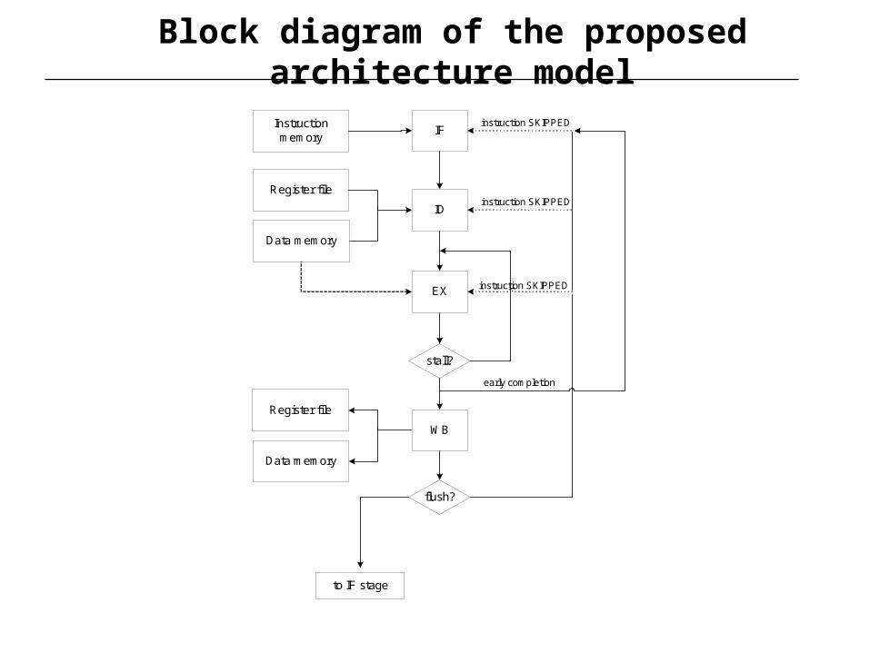
Block diagram of the proposed architecture model

IF

ID

EX

stall?

WB

flush?

Instructionmemory

Register file

Data memory

instruction SKIPPED

instruction SKIPPED

instruction SKIPPED

Register file

Data memory

early completion

to IF stage

The proposed approach for ASIP design space exploration

• Application analysis: extract weights for the coarse-level requirements

• Application description: the application is documented in basic blocks in the form of MOPs

• MOPs are defined only for the frequently executed operations satisfied by corresponding hardware resources

• Scheduling of the MOPs: the MOPs are scheduled into time steps, taking into account architecture characteristics, resource allocation and timing constraints

• Instruction generation: instructions are generated from time steps in the schedule. Possibility of multi-cycle instructions

• Performance estimation: the MOP description for the target application is simulated on the modified architecture model to evaluate the effect of the architecture changes

Performance estimation

• A retargetable cycle-accurate simulator is created for design verification and performance/power estimation

• Architecture changes are incorporated in the simulator

• The simulator is updated with the characteristics of the hardware resources

• Performance estimation: the simulator accounts for the cycle count, number of issued and executed instructions.

• Energy estimation: average power and total energy consumption are calculated by adding the contributions from each functional and storage resources

• Area estimation: count of equivalent gates

• The simulator utilizes pre-characterized resource models derived from PEAS-III framework

Outline





• Case study: ASIP design for an image compositing applicationCase study: ASIP design for an image compositing application

Case study: Image compositing

• Case study: Image compositing application (alpha blending) for the visual part of MPEG-4

• A common technique in computer graphics and visualization to perform simple compositing of digital images

• This version of the algorithm follows a block-based processing approach, and consists of two double-nested loops. A simple case is assumed with 1 foreground and 1 background objects of the same size

Application analysis for the case study

• The alpha blending algorithm is described in C code. Here is the corresponding pseudocode

for i in 0 to H/B, step B

for j in 0 to W/B, step B

for k in 0 to B, step 1

for l in 0 to B, step 1

temp = alpha*img_in1[B*i+k][B*j+l] +(255-alpha)*img_in2[B*i+k][B*j+l];

img_out[B*i+k][B*j+l] = (temp>>8);

endfor;

endfor;

endfor;

endfor;

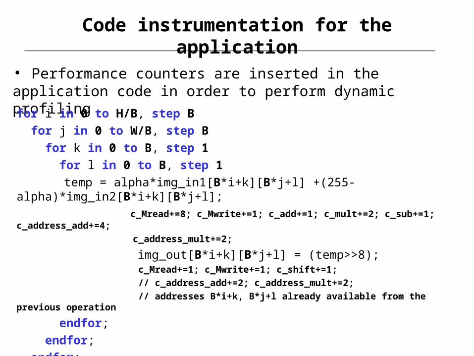
Code instrumentation for the application

• Performance counters are inserted in the application code in order to perform dynamic profiling

for i in 0 to H/B, step B

for j in 0 to W/B, step B

for k in 0 to B, step 1

for l in 0 to B, step 1

temp = alpha*img_in1[B*i+k][B*j+l] +(255-alpha)*img_in2[B*i+k][B*j+l];

c_Mread+=8; c_Mwrite+=1; c_add+=1; c_mult+=2; c_sub+=1; c_address_add+=4;

c_address_mult+=2;

img_out[B*i+k][B*j+l] = (temp>>8); c_Mread+=1; c_Mwrite+=1; c_shift+=1;

// c_address_add+=2; c_address_mult+=2;

// addresses B*i+k, B*j+l already available from the previous operation

endfor;

endfor;

endfor;

endfor;

Dynamic profiling results and discussion

• A result file is generated with the extracted information

RESULT FILE for Alpha Blending algorithm

Filename: ablend_c_report.txt

Parameters: H=288, W=352, B=8

-----------------------------------------------------------

Number of adds:101376

Number of multiplies:202752

Number of address stepping operations:115668

Number of address add operations:405504

Number of address multiply operations:202752

Number of memory element reads:912384

Number of memory element writes:202752

Number of subtracts:101376

Number of shifts:101376

Micro-operation description for the application

for l in 0 to B-1, step 1

temp = alpha*img_in1[B*i+k][B*j+l] +

(255-alpha)*img_in2[B*i+k][B*j+l];

…

endfor;

• The initial MOP description for the application movi Rix3, 0 movi Rfin3, 7loop3: mul R6, R3, Rix0 add R6, R6, Rix2 mul R7, R3, Rix1 add R7, R7, Rix3 mul R8, R6, R2 add R8, R8, R7 movi R13, 0 shl R13, R13, 8 ld R9, R8, R13 movi R13, 99 shl R13, R13, 8 ld R10, R8, R13 rsbi R6, R0, 255 mul R7, R0, R9 mul R11, R6, R10 add R12, R7, R11 … (MOPs for storing temp) addi Rix3, Rix3, 1 cmp Rix3, Rfin3 blt loop3

Baseline architecture for the image compositing ASIP

• In the first step, we derive a baseline architecture for the ASIP

• Architecture parameters: single ALU single-cycle array multiplier shifter with left/right shift capability single register file with 3 read ports and 1 write port dedicated adder for PC update local (on-chip) instruction and data memory

• The application is analyzed in MOPs and implemented by appropriate scheduling of these in time steps. MOPs in the same time step identify an instruction with needed resources

• The initial instruction set consists of 13 instructions (following table)

Baseline architecture for the image compositing ASIP(2)

• Initially, instruction and data sizes are restricted to 32 bits. Finally, we select 28-bit fixed length instructions and 24-bit datapath

• Since a full-sized array multiplier presents significant propagation delay, we have selected two-stage multiplier implementation

• Instructions present a CPI of 1 except: load register from memory (stall in EX stage, so 2 incremental cycles are required), multiply instruction (2 incremental cycles)

Extracted instruction set

• “Inst. Definition” column shows the instruction counterparts to which the micro-operations are mapped

Architectural modifications to the basic instruction set/ micro-architecture

• Modifications are applied to the initial specification of the ASIP and three different configurations are produced

Version 1: Effect of register file topology (additional register files are introduced to store the index values for the loops in the algorithm)

Version 2: Effect of implementing the multiply-add operation

Version 3: Effect of replacing chainable operations by single instructions (the packing of MOPs produces alternative instructions

• The effect of these modifications on cycle performance and energy consumption is evaluated in our cycle-accurate simulator

• The registers in the initial register file are reduced from 32 to 16 and 3 additional register files are used to store the running index, final and step values

• The index register files consist of 4 12-bit registers with 2 read and 1 write ports

• Tradeoffs in version 1 of the ASIP: For each register file, a separate address may be required, and this overhead has to be compensated by the reduction in energy consumption due to fewer storage bits The use of different data widths in the datapath requires the use of size-extension circuitry, which negatively affects propagation delay

• Results: The number of execution cycles is not affected Energy consumption is reduced by 20%

Version 1: Effect of register file topology (tradeoffs)

Version 2: Effect of the Multiply-Add operation

• The resulting architecture (version 1) is used as input to subsequent design space exploration steps

• Application analysis has identified a frequent pattern consisting of the MUL and ADD micro-operations

• A new instruction, MADD, is designed that incorporates the MUL and ADD micro-operations in the same control step

• An adder (in the ALU) and a multiplier were already included in the original configuration, so only minimal changes to the interconnection of these units are required

• Results: Reduction of 12% in the clock cycles and 17% in the energy consumption are observed (against version 1)

Version 2: Effect of the Multiply-Add operation (explanation)

• Pattern matching for the MUL-ADD micro-operation couple

• Baseline assembly code • Assembly code for version 2 of the ASIP

MUL R8, R6, R2

ADD R8, R8, R7MAC R8, R6, R2, R7

• Micro-operation description for the MAC operation

Instruction format: MAC Rd, Rs1, Rs2, Rs3 (D-format)

Action: Rd (Rs1*Rs2) + Rs3

Version 3: Effect of replacing chainable operations by single instructions

• The MOVI-SHL couple is replaced by a move immediate and shift left instruction (MVISL)

• An instruction for loop increment and conditional branch is inferred from an ADDI-CMP-BLT operation pattern (FOR instruction)

• The modifications required are the inclusion of a dedicated adder and multiplexing for calculating loop specifying the running index register, with final and step index registers implicitly encoded

• The average power consumption is indices

• In the FOR instruction definition, two register fields are saved, since only a single field is used for slightly increased due to the incorporation of additional hardware

• The number of machine cycles is reduced to the 50% of the initial configuration

• The energy consumption is reduced by a factor of 2.5

Version 3: Effect of replacing chainable operations by single instructions (explanation)

• Pattern matching for the MOV-SHL couple

• Baseline assembly code• Assembly code for version 3 of the ASIP

MOVI R13, 0SHL R13, R13, 8

MVISL R13, 0, 8

• Micro-operation description for the MVISL operation

Instruction format: MVISL Rd, #immed, #shamt

Action: Rd immed << shamt

shamt: shift amount (an immediate 5-bit value)

Version 3: Effect of replacing chainable operations by single instructions (expl. cont.)

• Pattern matching for the ADD-CMP-BLT triple

• Baseline assembly code • Assembly code for version 3 of the ASIP

ADDI Rix3, Rix3, 1 CMP Rix3, Rfin3BLT loop3

FOR Rix3, #loop3

• FOR instruction:

Instruction format: FOR Rd, #target_addr (I-format with Rs field unused)

Actions: Rd Rd + Rstp ; flags: Rd - Rfin ; if (flags): PC target_addr

“;” denotes concurrency in terms of control steps

Comparison

application specific instruction set processor design nikolaos kavvadias april 2003 (converted...

Documents

embedded systems design

asip design introduction

joint design of instruction

critical design concern

processors asips slide

embedded systems industry

target application

particular application