application of the momentary fourier transform to radar ... · application of the momentary fourier...

Budapest University of Technology and Economics

Department of Telecommunications

Application of the Momentary Fourier Transform to Radar Processing

Sandor Albrecht

Summary of the Ph. D. Dissertation

Advisors

Dr. Ian Cumming Department of Electrical and Computer Engineering

University of British Columbia, Vancouver, BC

Dr. Laszlo Pap Department of Telecommunications

Budapest University of Technology and Economics

Budapest, 2002

1

1 Introduction

Linear transformations, such as the discrete Fourier transform (DFT) are frequently used in digital signal processing, and their efficiency is very important. In applications where the DFT is applied to a signal, it is often desirable to use successive, possibly overlapping DFTs of smaller extent than the full length of the signal to obtain the spectrum coefficients. These transformations are normally off-line operations on blocks of data, requiring N samples of the signal before the transformation can be computed. The momentary Fourier transform (MFT) is a method of computing the DFT of a sequence in incremental steps. It can be computed using an efficient recursive formula, and it is useful in cases where the detailed evolution of the spectra of a discrete series is wanted, and in cases where only a few Fourier coefficients are needed. Uses of the incremental DFT were introduced by Papoulis in 1977 [1], and by Bitmead and Anderson in 1981 [5]. A detailed derivation of the momentary Fourier transform was given by Dudás in 1986 [6]. In 1991, Lilly gives a similar derivation, using the term “moving Fourier transform”, and uses the MFT for updating the model of a time-varying system [7]. A synthetic aperture radar (SAR) is a powerful sensor in remote sensing which is capable of observing geophysical parameters of the Earth’s (or another planet’s) surface, regardless of time, day and weather conditions [3]. SAR systems are extensively used for monitoring ocean surface patterns, sea-ice cover, agricultural features and for military applications such as in the detection and tracking of moving targets. A SAR transmits radar signals from an airborne or spaceborne antenna which is perpendicular to the flight direction of the platform which travels at a constant velocity. The back-scattered signal is collected by the antenna and stored in a raw format. Extensive signal processing is required on the ground to produce the output SAR image. The SPECtral ANalysis (SPECAN) SAR processing algorithm was developed in 1979 by MacDonald Dettwiler and Associates (MDA), as a multi-look version of the deramp-FFT method of pulse compression. In SPECAN, the received signals are multiplied in the time domain by a reference function, and overlapped short length DFTs are used to compress the data. In contrast, a precision processing algorithm such as the Range Doppler (RD) method requires both forward and inverse DFT operations, thus it is less computationally efficient. SPECAN is an efficient algorithm for moderate to low resolution processing and generally implemented in quick look processors for viewing of magnitude detected imagery data. Burst-mode operation is used in SAR systems, such as RADARSAT or ENVISAT, to image wide swaths, to save power or to reduce data link bandwidth. In this operational mode, the received data is windowed in a periodic fashion in the azimuth time variable, which results in a segmented frequency-time structure of its Doppler energy. This

2

frequency-time pattern requires special processing to maintain accurate focusing, consistent phase and efficient computing.

2 Research objectives

The objective of my research was to further develop the theory of the MFT, examine its properties and applications, and in particular, see what advantages it offers to SPECAN processing and to the short IFFT (SIFFT) burst-mode processing algorithm. I introduced the momentary matrix transform (MMT), and showed when the MMT takes the form of the DFT or the IDFT, the resulting MFT and IMFT have an efficient computational structure. The properties and computing efficiency of the MFT was also investigated. The azimuth FM rate of the received signal varies in each range cell, which leads to the issue of keeping the azimuth resolution and output sampling rate constant. I derived a tailor-made reduced MFT algorithm and showed what advantages the MFT method offers versus the FFT algorithms when they are applied to the SPECAN SAR processing algorithm. I investigated in details the properties of the received burst-mode data of the ScanSAR operation mode. I showed the effect of the Doppler centroid and the circular convolution on the Doppler history. I analyzed the properties of the input and output target space of the SIFFT algorithm and derived closed formulas for them. I defined the arithmetic of the SIFFT algorithm using IMFT and IFFT and showed how the IMFT algorithm can improve the computational efficiency of the SIFFT algorithm.

3 New results

Thesis 1: The momentary Fourier transformation pair [J1, J2, J3, C3]

The momentary Fourier transform (MFT) computes the DFT of a discrete-time sequence for every new sample in an efficient recursive form. I gave an alternate derivation of the MFT and IMFT using the momentary matrix transform (MMT) (Thesis 1.1) and examined the their properties and efficiency (Thesis 1.2). Thesis 1.1: Derivation of the momentary Fourier transformation pair from recursive matrix transformations

Let x be arbitrary discrete time sequence analyzed through an N-point window, ending at the current time i. In subsequent analyses, the window will be advanced one sample at a time. At sample i xi enters the window, while xi-N leaves the window. Let T be an NxN nonsingular matrix, which represent a linear transformation and has the inverse T-1. The sequence of index vectors is transformed by T at each sample. From the general

3

form of momentary matrix transform (MMT), I introduced the recursive form of the MMT:

i11 xTyTPTxTy ∆+== −

−ii i

(1)

In eqn. (1), P is the NxN elementary cyclic permutation matrix while ∆xi is the so-called adjustment vector made in the last row for the difference between the samples entering and leaving the window. Note, calculation of the newly transformed index vector yi in eqn. (1) is obtained from the previously transformed vector yi-1 and the difference between samples entering and leaving the window. The recursive MMT can be diagonalized and has the following diagonal form:

( )i-NiN- i

m

l

k

i xx

..

....

....

.

..

−+

��

�

�

��

�

�

= − 11

00

0

0

000

00

Tyy

λ

λλ

,

(2)

where TN-1 is the last column of the matrix T, k/N j2kk e=w πλ −= is the eigenvalue of P

and k, l, m ∈ {0,1,…,N-1}. I showed, if T performs the DFT, F (eqn. (3)) or the IDFT, F-1 (eqn. (4)), diagonal forms of the MMT can be obtained:

( )i-Ni

)(N

i

)-(N

-

-

ii--

i xx

w

.

w

w

w..

....

.w..

.w

..

= −

��

�

�

�

+

��

�

�

�

∆+=

−−

−

−

−

− 1

2

1

1

1

2

1

11

1

00

0

0

000

001

yxFyFPFy

(3)

( )Nii)-(N-

)(N

i)-(N-

)-(N-

i-

i--

i yy

w

.

w

w

w..

....

.w..

.w

..

=+= −

−

−−

−

−

−

��

�

��

�

�

+

��

�

��

�

�

∆

1

2

1

1

1

2

1

11

1

1

00

0

0

000

001

xyFxFPFx

(4)

4

Equation (3) expresses the recursive equation of the momentary Fourier-transform (MFT) [6, 7, 8]. The N-element vector yi contains the Fourier coefficients of the N-point sequence xi ending at sample i. Note that each spectral component yi,k can be calculated independently,

( )Niik,ik

i,kxxyw

y −−

− −+= 1

(5)

which increases efficiency if only a few frequency components need to be computed, as in the zoom transform. Also note that only one complex multiplication and two complex additions are needed to update each spectrum component. On the other hand, eqn. (4) is the dual of the MFT, the recursive inverse momentary Fourier-transform (IMFT), where the N-element vector xi contains the N-point time sequence and yi contains N Fourier coefficients ending at frequency bin i. Note that each sample in xi can also be obtained independently and the same twiddle factors, but in different order, can be used to calculate both the MFT and IMFT. Thesis 1.2: Comparison of MFT to FFT algorithms

Consider the case where N point DFTs are used to analyze an M-point complex-valued data record. If the window is shifted by q samples between each DFT application, where

1 ≤ q ≤ N, then M N

q1

−+ DFTs are needed to spectrum analyze the record, in the case

of FFT. If the MFT is applied, M MFTs are needed, because the spectrum coefficients have to be calculated in each time samples, irrespectively of the value of q. I showed that the number of shift between DFTs when the MFT is more efficient than the radix-2 FFT is

[ ](N)N-)-N(M

(N)NN)(Mq

cMFT

2

2

log518

log5−<

(6)

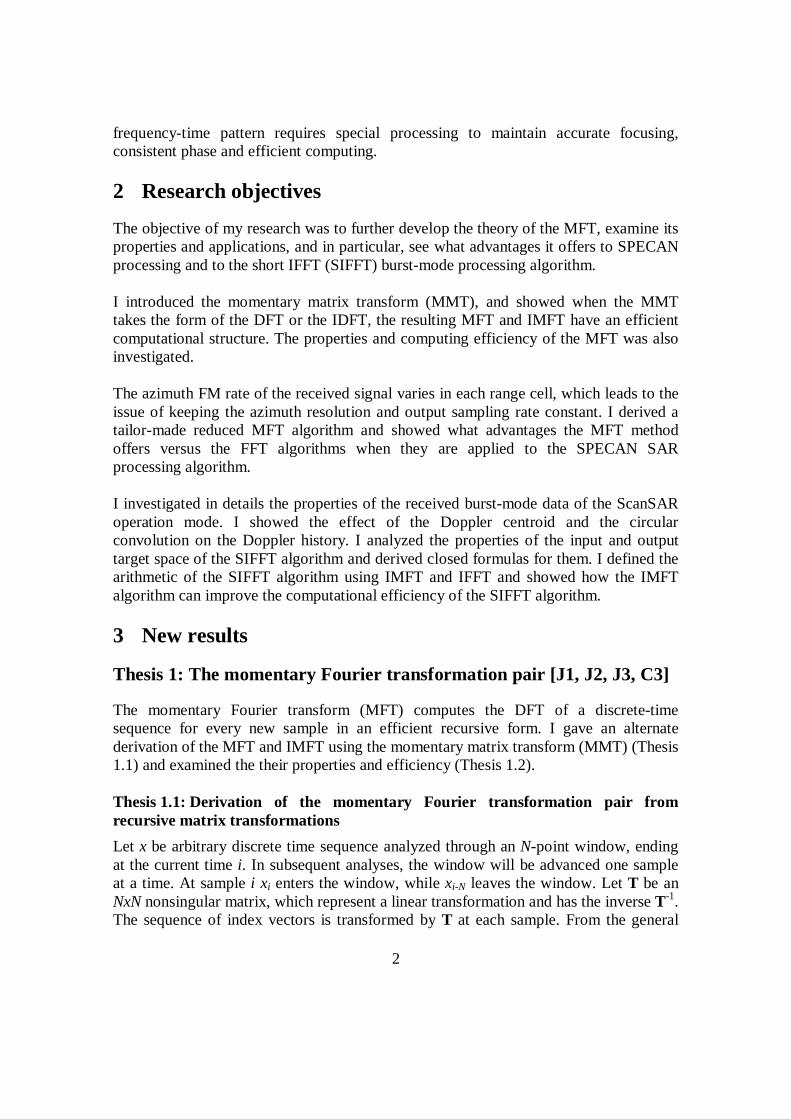
As we can see from eqn. (6), qMFT is function of the length of the data record (M), the size of the window (N) and the calculated MFT spectrum coefficients (Nc). In Figure 1, the shift between DFTs when the MFT is more efficient is shown as a function of the window length, with two values of Nc. The full MFT is more efficient compared to the radix-2 FFT, if the shift between DFTs is very small (qMFT ≤ 5), while for the reduced MFT (Nc = N/4), the MFT is more efficient even for larger values of shift. The computational load for small amount of shifts is given in Figure 2.

5

100 200 300 400 500 600 700 800 900 1000

2

4

6

8

10

12

14

16

18

20

22

24

26

Number of shift between DFTs when MFT is more efficient than FFT

Window size [sample]

Shif

t be

twee

n D

FT

s [s

ampl

e]

Total samples analyzed = 25000

1/4N MFT

Full MFT

Figure 1 Shift between DFTs when the MFT is more efficient

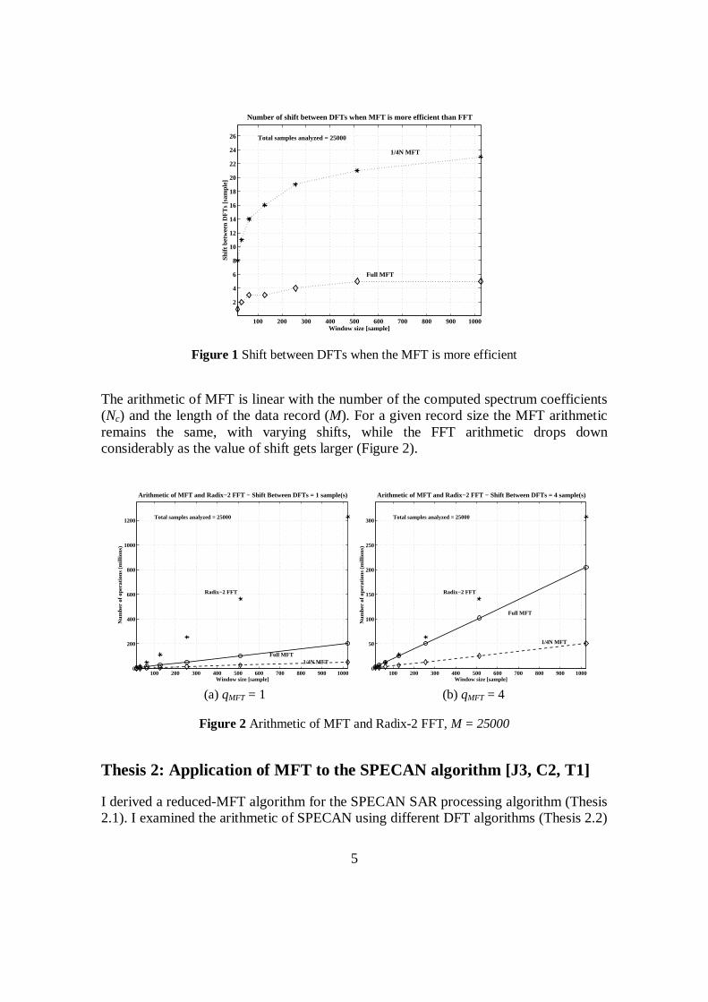
The arithmetic of MFT is linear with the number of the computed spectrum coefficients (Nc) and the length of the data record (M). For a given record size the MFT arithmetic remains the same, with varying shifts, while the FFT arithmetic drops down considerably as the value of shift gets larger (Figure 2).

100 200 300 400 500 600 700 800 900 10000

200

400

600

800

1000

1200

Arithmetic of MFT and Radix−2 FFT − Shift Between DFTs = 1 sample(s)


Num

ber

of o

pera

tions

(m

illio

ns)


Radix−2 FFT

Full MFT1/4N MFT

100 200 300 400 500 600 700 800 900 1000

0

50

100

150

200

250

300

Arithmetic of MFT and Radix−2 FFT − Shift Between DFTs = 4 sample(s)


Num

ber

of o

pera

tions

(m

illio

ns)


Radix−2 FFT

Full MFT

1/4N MFT

(a) qMFT = 1 (b) qMFT = 4

Figure 2 Arithmetic of MFT and Radix-2 FFT, M = 25000

Thesis 2: Application of MFT to the SPECAN algorithm [J3, C2, T1]

I derived a reduced-MFT algorithm for the SPECAN SAR processing algorithm (Thesis 2.1). I examined the arithmetic of SPECAN using different DFT algorithms (Thesis 2.2)

6

and showed what advantages the MFT has compared to the FFT algorithms when they are applied to SPECAN (Thesis 2.3). Thesis 2.1: Reduced MFT algorithm for SPECAN

The azimuth FM rate of the received SAR signal is inversely proportional to range, so it changes as the range varies in each cell. In order to keep the resolution and output sampling rate constant across the swath, there is a need to choose different DFT lengths for SPECAN, with the DFT length increasing one sample at a time as range increases. The effect of the varying range on the FM rate and the desired DFT length for a typical airborne radar case is shown in Figure 3. Note that there is a need for a wide range of DFT lengths to keep the resolution constant through the whole swath.

6 8 10 12 14 16 18 2020

40

60

80

100Azimuth FM Rate and DFT Length in SPECAN

Range [Km]

Azi

mut

h F

M R

ate

[Hz/

s]W

indow size [sam

ples]

Azimuth FM Rate→

←DFT length

6 8 10 12 14 16 18 20100

200

300

400

500

Figure 3 Azimuth FM rate and the DFT length with varying range, airborne SAR case

The Radix-2 FFT algorithm can be only used when the DFT length is a power of two (Figure 3, N = 256). In other cases of window length a mixed-radix FFT algorithm is used to achieve efficiency only for highly composite N. It means, for each different DFT a different FFT algorithm should be implemented within the SPECAN processor, which makes the architecture rather complex when many different FFT lengths are needed. In contrast to FFT algorithms, the structure and the efficiency of the MFT does not rely upon the size of the DFT. The same simple algorithm can be used to calculate all of the necessary DFTs during the azimuth compression. In SPECAN, during the DFT extraction only a portion of the spectrum coefficients - the good output samples (G) - are used at the same time to obtain the compressed data. Although the amount of these spectrum components remains the same through the processing, their position changes with the DFTs. So, the conventional form of the

7

reduced-MFT algorithm cannot be used. The sub-band of the calculated spectrum coefficients has to change its positions in the frequency domain in phase with position of the good output samples. I gave a detailed derivation of the reduced-MFT algorithm for SPECAN and showed how many real operations are needed to process the whole processing region with the reduced MFT (eqn (7)).

( )

[ ] [ ] ( )[ ]( )2828128

1 221

+−++�� +−++=

+�� +−+=

LGqLNq

NMGN

MFTOPSMFTOPSq

NMMFTOPSMFTOPS OLDDFTNEWDFTDFT

(7)

Although eqn. (7) looks rather complex, the implementation of the reduced MFT algorithm is the same as the full MFT algorithm, except the timing and synchronization of the sub-band of the calculated spectrum coefficients. Thesis 2.2: Arithmetic of SPECAN

Figure 4 shows the number of operations of the SPECAN azimuth compression for the airborne radar case, covering the range of DFT lengths defined in Figure 3. In this figure, the arithmetic of the direct DFT algorithm, the full and reduced MFT, the mixed-radix and the radix-2 FFT are compared. In Figure 4, it can be seen that the FFT arithmetic is generally smaller than the MFT arithmetic, although it is quite variable as the radix changes throughout the range swath.

150 200 250 300 350 400 4500

2

4

6

8

10

12

14

16

18

20

DFT Operations in SPECAN

Window size [samples]

Num

ber

of O

pera

tion

s (m

illio

ns)

DFT Mixed−radix FFTFull MFT Reduced MFT Radix−2 FFT

Figure 4 Arithmetic of SPECAN azimuth compression with different DFT algorithms

8

Note that the arithmetic of the full and reduced MFT is more uniform in contrast with the arithmetic of the mixed-radix FFT algorithms. Also note, that the arithmetic of the mixed-radix algorithm is equal to the direct DFT if the window length is a non-composite number (i.e. prime) and the radix-2 FFT algorithm can be used only once during the process, when the DFT length is 256 samples. Thesis 2.3: Output sampling rate of SPECAN

Beside the complexity and computational efficiency, another important issue in the SPECAN algorithm to keep the output sampling rate constant. In other words, targets which are T seconds apart in azimuth input time must appear T seconds apart in the output data. It was shown in [11] that the azimuth output sample rate is

Hz a

aout F

NKF =

(8)

where Ka is the azimuth FM rate and Fa is the azimuth sampling rate. The output sampling rate strongly depends on the azimuth FM rate, so when it changes throughout the swath, there is a need for slowly varying DFT length to keep the output sampling rate constant. Figure 5 shows Fout as the function of range, when MFT and radix-2 FFT is applied in the SPECAN algorithm to an airborne system. Note when the MFT algorithm is applied, the output sampling rate is more uniform, while when the radix-2 FFT is used it has a large migration. The reason of this migration is that only two transformation lengths 256 and 512 can be used when the radix-2 FFT is applied to SPECAN.

6 8 10 12 14 16 18 20

40

45

50

55

60

65

70

75

Output Sampling Rate

Range [Km]

Out

put S

ampl

ing

Rat

e [H

z]

MFT

Radix−2 FFT: N = 256 and 512

Figure 5 The output sampling rate of the SPECAN algorithm

9

Thesis 3: Properties of burst-mode SAR data processing and the SIFFT algorithm [J1, J2]

I gave detailed description of the properties of burst-mode data processing and the SIFFT algorithm. I showed the effect of the frequency domain convolution on the Doppler history of burst-mode data (Thesis 3.1), and how the Doppler history is effected when the aperture contains an odd or even number of complete bursts (Thesis 3.2). I derived the shift between the spectra of two consecutive compressed targets and two consecutive IFFTs in the Doppler history (Thesis 3.3), and gave explicit formulas for both the input and output target space of the SIFFT algorithm (Thesis 3.4). Thesis 3.1: Effect of the circular convolution on the Doppler history

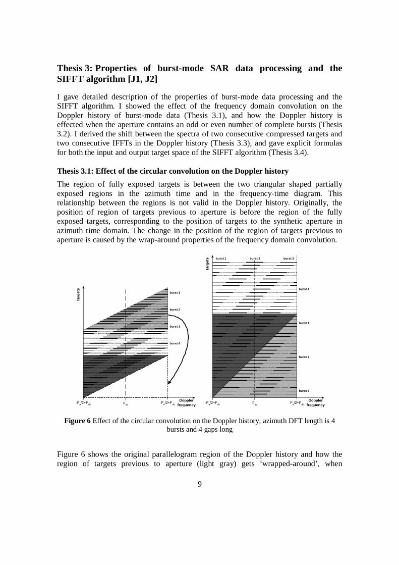
The region of fully exposed targets is between the two triangular shaped partially exposed regions in the azimuth time and in the frequency-time diagram. This relationship between the regions is not valid in the Doppler history. Originally, the position of region of targets previous to aperture is before the region of the fully exposed targets, corresponding to the position of targets to the synthetic aperture in azimuth time domain. The change in the position of the region of targets previous to aperture is caused by the wrap-around properties of the frequency domain convolution.

burst 1

burst 2

burst 3

burst 4

DopplerfrequencyFdc

-Fa/2+Fdc Fa/2+Fdc

targ

ets

burst 1 burst 2 burst 3

Fdc

Dopplerfrequency

burst 4

burst 1

burst 2

burst 3

-Fa/2+Fdc Fa/2+Fdc

targ

ets

Figure 6 Effect of the circular convolution on the Doppler history, azimuth DFT length is 4 bursts and 4 gaps long

Figure 6 shows the original parallelogram region of the Doppler history and how the region of targets previous to aperture (light gray) gets ‘wrapped-around’, when

10

frequency-domain circular convolution [4] is used instead of time-domain linear convolution. Note that targets in the fully exposed region get compressed into different output cells, while when the top triangle gets wrapped-around different targets are compressed into the same cell depending on which Doppler sub-band (e.g. burst 1 or burst 3) is used. This property of the wrapped-around target Doppler history has to be taken under consideration, when extracting targets during burst-mode signal compression. Thesis 3.2: Effect of the number of complete burst in the synthetic aperture

Usually target exposures (burst bandwidths) closest to the Doppler centroid are used for target extraction in burst-mode data processing. Figure 7 (a) and (b) show the Doppler history of the same aperture when it contains three or four full bursts and the length of the azimuth DFT is equal to the synthetic aperture (Nfft = Na). The processing region in the Doppler frequency domain is three burst-bandwidth wide (3Fburst Hz) around the Doppler centroid, independently of the number of burst in the aperture. The start and end point of this region are

[Hz] 5.12

[Hz] 5.12

burstHzendburstHza

end

burstHzstartburstHza

start

FkFk

P

FkFk

P

=��

��+=

=��

��−=

(9)

where ka equals the number of burst lengths (bursts + gaps) in the aperture (i.e. Fa = ka⋅Fburst Hz). It is assumed that there are an integer number of bursts and gaps in the aperture, and the first interval is a burst.

burst 1

burst 2

burst 3

burst 1 burst 2 burst 3

(Fdc)Doppler

frequency(-Fa/2+Fdc) (Fa/2+Fdc)

1Fburst 2Fburst 3Fburst 4Fburst0 5Fburst

targ

ets

processing region

burst 1 burst 2 burst 3 burst 4

burst 1

burst 2

burst 3

Dopplerfrequency

burst 4

(Fdc)

(-Fa/2+Fdc) (Fa/2+Fdc)

1Fburst 2Fburst 3Fburst 4Fburst0 7Fburst5Fburst 6Fburst

targ

ets

processing region

(a) odd number of bursts (3 bursts) (b) even number of bursts (4 bursts)

Figure 7 The Doppler history when there are odd or even number of bursts in the synthetic aperture

11

It can be shown that if there is an odd number of bursts in the aperture then kstart is odd, while if the aperture contains an even number of bursts, it is even. This also means that right around the Fdc there is a burst in the even case and a gap in the odd case. This property affects the pattern of targets exposure in the processing region in the following way: • If there is an odd number of complete bursts in the aperture, the first group of bursts

starts in the middle and ends at the beginning of the processing region (Figure 7 (a)). The second group starts at the end and scans through the whole interval. The last target group (from targets previous to aperture) also starts at the end but it lasts only until the middle of the region. Note that the first and last group contain only half the number of targets than the other groups.

• If there is an even number of complete bursts in the aperture, all target groups have the same length, start at the end, and last until the beginning of the processing region (Figure 7 (b)).

Thesis 3.3: Shift between output targets and IFFTs

The shift between the spectra of two consecutive compressed targets (qoutar) in the Doppler history is shown in Figure 8 and can be obtained as follows:

IFFTa

FFTa

IFFT

FFTHztarHzoutar NF

NK

N

Nqq == [Hz]

��=��

��=��

∆=

IFFTa

FFTa

a

FFTHzoutar

Hzoutarbinoutar NF

NKround

F

Nqround

f

qroundq 2

2

[frequency bin]

(10)

The shift between two consecutive IFFTs (qifft)in the SIFFT algorithm is also indicated in Figure 8 and can be obtained as follows. All IFFTs start at the beginning of a burst’s spectra of a target, so qifft can be divided into integer number of qoutar (Figure 8). The number of qoutar in the shift between two consecutive IFFTs is

1

+�� −

=binoutar

binburstIFFToutar q

FNfloorQ

(11)

Using eqn. (11) the shift between two consecutive IFFTs (qifft) is

�� +��

�� −= 1

binoutar

binburstIFFTbinoutarifft q

FNfloorqq [frequency bin]

(12)

12

When NIFFT Min is used, the shift between IFFTs is equal to the shift between output targets (qifft = qoutar). When NIFFT gets larger, qifft also gets larger, thus fewer IFFTs are needed to compress all targets (i.e. one IFFT extracts more targets).

Fdc

Dopplerfrequency

-Fa/2+Fdc Fa/2+Fdc

qifft qoutar

IFFT2

IFFT1

Figure 8 Shift between two consecutive IFFTs

Thesis 3.4: Input and output target space

I showed how many targets from an azimuth DFT can be compressed using the SIFFT algorithm. During the investigation it was assumed that targets having a complete burst exposure in the processing region are being compressed. The number of processed targets from previous to aperture (ITSbefore) is independent from the azimuth DFT length (NFFT), and it can be shown that

2ba

before

NNITS

+=

(13)

The number of extracted fully exposed targets (ITSfully) is the same as the number of targets compressed in continuous mode processing and, depends linearly on the azimuth DFT length:

1+−= aFFTfully NNITS

(14)

When the minimum NFFT is used, the number of extracted targets from after aperture (ITSafter) is equal to ITSbefore. As the azimuth DFT gets larger, ITSafter gets smaller until another full gap and full burst is not covered by the DFT. During this 2Nb interval, ITSafter depends linearly on NFFT, and can be obtained as follows:

13

�� −

−+

=b

aFFTb

baraft N

NNfractionN

NNITS

22

2e

(15)

The whole input target space (ITS) for a given azimuth DFT (NFFT) is equal to the sum of the number of processed targets in the three regions (ITS = ITSbefore + ITSfully + ITSafter), and can be expressed as follows:

�� −

+++=b

aFFTbba N

NNfloorNNNITS

221

(16)

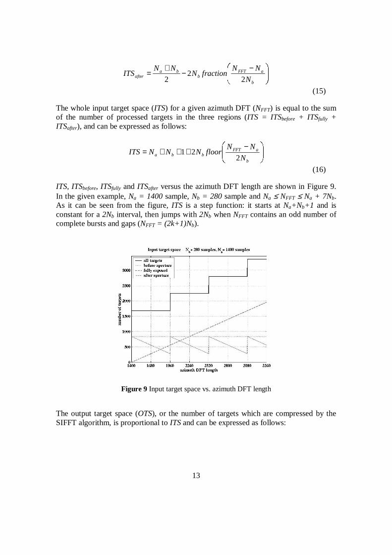
ITS, ITSbefore, ITSfully and ITSafter versus the azimuth DFT length are shown in Figure 9. In the given example, Na = 1400 sample, Nb = 280 sample and Na ≤ NFFT ≤ Na + 7Nb. As it can be seen from the figure, ITS is a step function: it starts at Na+Nb+1 and is constant for a 2Nb interval, then jumps with 2Nb when NFFT contains an odd number of complete bursts and gaps (NFFT = (2k+1)Nb).

Figure 9 Input target space vs. azimuth DFT length

The output target space (OTS), or the number of targets which are compressed by the SIFFT algorithm, is proportional to ITS and can be expressed as follows:

14

( ) ��

��

��

��

��

−+++=⋅=FFT

IFFT

b

aFFTbbaSIFFT N

N

N

NNNNNfloorITSfloorOTS

221ρ

(17)

where ρSIFFT is the output resolution of the SIFFT algorithm. The number of compressed targets in the three regions can be obtained similarly to OTS:

�� +

=FFT

IFFTbabefore N

NNNfloorOTS

2

( ) 1+�� −=

FFT

IFFTaFFTfully N

NNNfloorOTS

��

��

��

��

−−+=FFT

IFFT

b

aFFTb

baraft N

N

N

NNfractionN

NNfloorOTS

22

2e

(18)

Thesis 4: Efficiency of the SIFFT algorithm [J1, J2, J3 C1]

I examined the arithmetic and the efficiency of the SIFFT algorithm using the IMFT and mixed-radix IFFT algorithms. I gave explicit formulas for the arithmetic of SIFFT and showed how it depends on the azimuth DFT length. I also investigated the efficiency of the SIFFT when it is applied to Envisat burst-mode data. Thesis 4.1: Arithmetic of SIFFT

The processing region of a burst-mode processing algorithm is three burst-bandwidth (3Fburst bin) long in the Doppler history. Thus both the IFFT and IMFT algorithms are applied only in this region when they are used in the SIFFT algorithm. There is qifft (eqn. (12)) shift between consecutive IFFTs to compress all targets in a 3Fburst bin long region. Than the number of IFFTs applied in the processing region is

��

�+−= 1

3

ifft

IFFTbinburstIFFT q

NFceilNUM

(19)

The number of operations needed to compress all targets using the IFFT algorithm is

15

IFFTIFFT Nifft

IFFTbinburstNIFFTIFFT NOP

q

NFceilNOPNUMNOP �

��

��

�+−=⋅= 1

3

(20)

where IFFTNNOP is the number of operations needed for one N sample long mixed-radix

IFFT. IFFTNNOP is smaller when N is a higher composite number. If N is power of 2

(radix-2 IFFT) than ( )NNNOPIFFTN 2log5= .

In case of IMFT with a NIMFT long window, NOPIMFT = M(8NIMFT + 2) real operations are needed to process an M-point complex data record. In the case of 2-beam burst processing M = 3Fburst bin, so the arithmetic of the IMFT algorithm is

)28(3 += IMFTbinburstIMFT NFNOP

(21)

Note that both formulas in eqn. (20) and eqn. (21) depend on the azimuth DFT length (NFFT) in the following way: NOPIFFT through NIFFT, Fburst bin and qi fft, while NOPIMFT through NIMFT. Thesis 4.2: Efficiency vs. azimuth DFT length

During the arithmetic calculation, parameters of the ideal target simulation given in Table 1 are used with the following azimuth DFT interval: 1960 ≤ NFFT ≤ 2519. First, we make the IFFT and IMFT window length to the minimum (NIFFT = NIMFT = Fburst bin), thus there is only one window length to choose from in the IFFT and IMFT algorithms. Secondly, we consider the case when the IFFT and IMFT window length is allowed to be up to four samples longer than the minimum (i.e. Fburst bin ≤ NIFFT and NIMFT ≤ Fburst

bin + 4). This allows some flexibility in choosing a favorable (more efficient) IFFT window from five different window sizes, at the expense of a small decrease in SNR.

Processing parameter Value Unit

Azimuth sampling frequency (Fa) 1673.32 Hz

Azimuth FM rate (Ka) -2000 Hz/s

Doppler Centroid (Fdc) 447.1 Hz

Synthetic aperture length - 3 bursts-2 gaps (Na) 1400 samples

Burst length (Nb) 280 samples

Table 1 Parameters of ideal target simulation

It can be seen from Figure 10 that the arithmetic of the IFFT algorithm is quite variable depending upon the composition of the NIFFT length. The IMFT arithmetic is much

16

smoother and it is a quadratic function of the azimuth DFT length, (eqn. (21), NIMFT = Fburst). It is also seen from the figure that the IMFT algorithm is more efficient in both cases, even if there is an option to choose a more suitable window length for the IFFT algorithm.

2000 2050 2100 2150 2200 2250 2300 2350 2400 2450 25000

50

100

150

200

250Arithmetic of IFFT and IMFT − burst = 280 samples, Synth. Ap. = 1400 samples

azimuth DFT length

num

ber

of o

pera

tions

(m

illio

ns)

IFFTIMFT

(a) minimum IFFT length is used

2000 2050 2100 2150 2200 2250 2300 2350 2400 2450 25000

5

10

15

20

25

Arithmetic of IFFT and IMFT − burst = 280 samples, Synth. Ap. = 1400 samples

azimuth DFT length

num

ber

of o

pera

tions

(m

illio

ns)

IFFTIMFT

(b) 5 IFFT length to choose from

Figure 10 Arithmetic of the IFFT and IMFT algorithm vs. azimuth DFT

The output target space can be considered constant for a 2Nb interval in the azimuth DFT domain. In the example in Figure 10, this interval is 560 NFFT long, starts at NFFT = 1960 and ends at NFFT = 2519. Within this interval the azimuth DFT length

17

corresponding to the most efficient IMFT or IFFT length can be used, without affecting the output target space. In Figure 10, the minimum of the arithmetic of the IMFT and the IFFT are also indicated with an asterisk. In the first case (Figure 10 (a)), the IFFT is most efficient when the azimuth DFT length is 2023 samples long , while in the second case (Figure 10 (b)) when NFFT = 2003 samples . As it can be seen from eqn. (20) NOPIFFT is smaller when a larger NIFFT is used and/or when

IFFTNNOP is smaller. When

NFFT = 2003, both conditions are satisfied to get the arithmetic lower: the NIFFT gets larger from 401 to 405 samples and the new window size is a higher composite number, thus

IFFTNNOP is smaller. The investigation to find a more efficient NIFFT for a given

azimuth DFT length has to be performed for each DFT size in the 2Nb interval. Then the most efficient IFFT window length’s arithmetic for the given DFT length has to be compared to the arithmetic of the most efficient window lengths corresponding to other DFT sizes. This searching algorithm is rather complex, and can take a long time. The arithmetic of the IMFT is directly proportional to NIMFT, so to have the best efficiency, NIMFT min should be used for each azimuth DFT length. It becomes a quadratic function of NFFT when NIMFT min is used. In this case, in a 2Nb long azimuth DFT interval the minimum of the IMFT arithmetic is always at the beginning of the interval (Figure 10). So, at any azimuth DFT length which consists of an odd number of burst lengths (i.e. NFFT = (2k+1)Nb), the IMFT algorithm is the most efficient for the next 2Nb long NFFT interval. Thesis 4.3: Efficiency of SIFFT when applied to ENVISAT

During the Envisat efficiency evaluation, we choose the IFFT and IMFT lengths on the principles that we want:

• maximum SNR at near range, • minimum sampling rate at near range, and • the sampling rate constant with range,

and we set the azimuth DFT length (NFFT ) to be 3200 and 4096 samples long. First, we make NIFFT and NIMFT as small as possible at near range (i.e. NIFFT = NIMFT = Max Fburst bin), and have it stay the same with range, even though the burst bandwidth decreases with increasing range. Thus there is only one window length to choose from for the IFFT and the IMFT algorithms. Second, we consider the case where the IFFT is allowed to be up to 4 samples longer than the minimum (i.e. Max Fburst bin ≤ NIFFT < Max Fburst bin + 4), while the IMFT length remains the same (i.e. NIMFT = Max Fburst bin). This allows some flexibility in choosing a favorable IFFT length from five different window sizes, at the expense of a small decrease in SNR. In Figure 11, the average millions of operations (MOPS) is shown for all Envisat swathes when the azimuth DFT is 3200 and 4096 samples long. The arithmetic of the

18

IMFT algorithm is the same in Figure 11 (a) and (b), and in Figure 11 (c) and (d) respectively, because the azimuth DFT length is the same, and NIFFT Min is used in the calculations. The trend of the arithmetic of the IMFT is similar in both NFFT cases, while the IFFT arithmetic is quite variable, depending upon the composition of the IFFT window length. When NFFT = 3200, the IMFT is more efficient for most of the swathes even if there is an option to chose a suitable window length for the IFFT algorithm. When NFFT = 4096, the IMFT is almost always better than the IFFT if only NIFFT Min can be used. When there is a possibility to choose a favorable IFFT length, the IFFT is more efficient for all the swathes except one, because there is a greater possibility of finding a high composite number in the neighborhood of NIFFT Min.

IS1IS2 IS4 IS6 IS3 IS5 IS70

10

20

30

40

50

60

Envisat swathes − number of IFFT windows to choose from = 1, NFFT

= 3200

Envisat swath

aver

age

MO

PS

per

swat

h

IFFTIMFT

(a) minimum IFFT length is used, NFFT = 3200


1

2

3

4

5

6


= 3200

Envisat swath

aver

age

MO

PS

per

swat

h

IFFTIMFT

(b) 5 IFFT lengths to choose from, NFFT = 3200

19


20

40

60

80

100

120


= 4096

Envisat swath

aver

age

MO

PS

per

swat

h

IFFTIMFT

(c) minimum IFFT length is used, NFFT = 4096


1

2

3

4

5

6

7


= 4096

Envisat swath

aver

age

MO

PS

per

swat

h

IFFTIMFT

(d) 5 IFFT lengths to choose from, NFFT = 4096

Figure 11 Arithmetic of the SIFFT when it is applied to Envisat AP burst mode operation

4 Application of new results

The MFT/IMFT transformation pair can provide more efficient computation of the DFT when:

• DFTs are highly overlapped, • only a few Fourier coefficients are needed,

20

• a specific, non-composite DFT length is needed, and they can be useful in different applications of signal processing such as:

• on-line computations in real-time spectral analysis, • on-line signal identification and detection, • speech processing and • radar and sonar processing.

Although, the MFT does not improve the computational efficiency of the SPECAN algorithm, except at the finest resolutions, it has the following advantages over the radix-2 and mixed-radix FFT when they are applied to SPECAN:

• The MFT has consistent computing load as the DFT length changes.

• It is easier to implement the MFT algorithm for variable window length. The architecture of a SPECAN processor using MFT is less complex, because the same MFT algorithm can be used for the different window lengths.

• The full radar resolution can be achieved, because the full Doppler spectrum of the targets can be used for the compression by using high-overlapped DFTs.

• The output sampling rate of SPECAN is more uniform.

The detailed description of the properties of Doppler history and SIFFT algorithm can be used for the architecture design of a burst mode SAR processor using the SIFFT algorithm. The IMFT algorithm can improve the computational efficiency of the SIFFT algorithm and has the following advantages when it is applied to the SIFFT algorithm:

• For a given azimuth DFT length, the IMFT algorithm is most efficient when the burst bandwidth (i.e. NIMFT min) is used. So, beside the efficiency targets with maximum SNR are compressed.

• The IMFT arithmetic is smooth and it is a quadratic function of the azimuth DFT length opposite to the arithmetic of the IFFT algorithm which is quite variable depending upon the composition of the window length.

• It is easier to implement the IMFT algorithm for different burst and NFFT lengths, because the same IMFT algorithm can be used for the different window lengths.

Acknowledgement

First of all, I would like to thank my mother and my wife for providing consistent support and encouragement throughout my research and studies. Without their love and care this work would not have been completed. I would like to thank Dr. Jozsef Dudas for the momentary Fourier transform and his guidance in my scientific career.

21

I would like to thank Dr. Ian Cumming, for his supervision and academic guidance, as well as providing the opportunity to continue my research of momentary Fourier transform in the field of synthetic aperture radar processing. I am grateful to Dr. Miklos Boda and Dr. Laszlo Pap for the academic and personal support throughout my work.

References

[1] A. Papoulis, Signal Analysis. McGraw-Hill, 1977

[2] G. Strang, Linear Algebra and Its Applications. Saunders College Publishing, Third Edition, 1988

[3] J. Curlander and R. McDonough, Synthetic Aperture Radar: System and Signal Processing. Wiley, New York, 1991.

[4] J. G. Proakis and D.G. Manolakis, Digital Signal Processing. Prentice Hall, Third Edition, 1996

[5] R. R. Bitmead and B. D. O. Anderson, "Adaptive frequency sampling filters," IEEE Trans. On Circuits and Systems, vol. CAS-28, pp. 524-534, June 1981.

[6] J. Dudás, The Momentary Fourier Transform. Ph.D. thesis, Technical University of Budapest, 1986.

[7] H. Lilly, ”Efficient DFT-based model reduction for continuous systems”, IEEE Trans. on Automatic Control, vol.36, pp. 1188-1193, Oct. 1991.

[8] B. G. Sherlock and D. M. Monro, “Moving discrete Fourier transform”, IEE Proceedings-F, vol. 139, pp. 279-282, Aug. 1992.

[9] K. Tomiyasu, “Tutorial Review of Synthetic-Aperture Radar (SAR) with Applications to Imaging of Ocean Surface, Proceedings of IEEE, Vol. 66, No. 5, pp. 563-583, May 1978

[10] I. Cumming and J. R. Bennett, "Digital processing of SEASAT SAR data", IEEE 1979 International Conference on Acoustic, Speech and Signal Processing, (Washington, D.C., USA), April 2-4, 1979.

[11] I. Cumming and J. Lim, “The design of a digital breadboard processor for ESA remote sensing satellite synthetic aperture radar” , technical report, MacDonald Dettwiler, Richmond, BC, Canada, July 1981. Final report for ESA Contract No. 3998/79/NL/HP(SC).

22

[12] J. R. Benett, I. Cumming and R. M. Wedding, “Algorithms for Preprocessing of Satellite SAR Data” , Proceedings of ISPRS Commission II. Symposium, (Ottawa, Canada), Aug. 30 – Sept. 3, 1982

[13] M. Sack, M. Ito, I. Cumming, “Application of Efficient Linear FM Matched Filtering Algorithms to SAR Processing” , IEEE Proc-F, vol.132, no. 1, pp. 45-57, 1985.

[14] T. Ngo and C. M. Vigneron, “Project Report: UBC SQLP v.1.7.” , technical report Radar Remote Sensing Group, Electrical and Computer Engineering, University of British Columbia, 1995.

[15] F. Wong, “Processing Envisat AP mode with Range Doppler algorithm”, technical report, MacDonald Dettwiler, Richmond, BC, Canada, January 1996.

[16] I. Cumming Y. Guo and F. Wong, “Analysis and Precision Processing of Radarsat ScanSAR Data” , Geomatics in the Era of Radarsat, GER’97, (Ottawa, Canada), May 25-30, 1997.

[17] F. Wong, D. Stevens and I. Cumming, “Phase-Preserving Processing of ScanSAR Data with Modified Range Doppler Algorithm”, Proceedings of the International Geoscience and Remote Sensing Symposium, IGARSS’97, (Singapure), pp.725-727, August 3-8, 1997.

[18] I. Cumming Y. Guo and F. Wong, “A Comparison of Phase-Preserving Algorithms for Burst-mode ScanSAR Data Processing” , Proceedings of the International Geoscience and Remote Sensing Symposium, IGARSS’97, (Singapure), pp.731-733, August 3-8, 1997.

[19] I. Cumming Y. Guo and F. Wong, “Modifying the RD Algorithm for Burst-mode SAR Processing” , Proceedings of the European Conference on Synthetic Aperture Radar, EUSAR’98, (Friedrichshafen, Germany), pp.477-480, May 25-27, 1998.

Publications

Journal Papers [J1] S. Albrecht, "Börsztmódusú, szintetikus apertúrájú radar (SAR) jelek feldolgozása momentán Fourier-transzformáció alkalmazásával", Híradástechnika, LVI. vol 2001/10, pp. 31-42, December 2001.

[J2] S. Albrecht, "Application of momentary Fourier transform to burst-mode SAR processing", Híradástechnika, LVI. vol 2001/9, pp. 49-60, December 2001.

[J3] S. Albrecht and I. Cumming, “Application of Momentary Fourier Transform to SAR Processing” , IEE Proceedings: Radar, Sonar and Navigation, 146(6), pp. 285-297, December 1999.

23

Conference Papers [C1] S. Albrecht and I. Cumming, “The Application of Momentary Fourier Transform to SIFFT SAR Processing” , Proceedings of the IEEE-SP International Symposium on Time-Frequency and Time-Scale Analysis, (Pittsburgh, USA) October 7-9, 1998.

[C2] S. Albrecht and I. Cumming, “Application of Momentary Fourier Transform to the SPECAN SAR Processing Algorithm”, Proceedings of the IX. European Signal Processing Conference, EUSIPCO’98, (Rhodes, Greece) September 8-11, 1998.

[C3] S. Albrecht, I. Cumming and J. Dudás, “The momentary Fourier transformation derived from recursive matrix transformations” , Proceedings of the 13th International Conference on Digital Signal Processing, DSP’97, (Santorini, Greece) vol. 1, pp. 337-340, 2-4 July, 1997.

Technical Report [T1] S. Albrecht, “The Momentary Fourier Transform and Its Application to the SPECAN SAR Processing Algorithm”, technical report SA-97-01, Radar Remote Sensing Group, Electrical and Computer Engineering, University of British Columbia, September 1997.

application of the momentary fourier transform to radar ... · application of the momentary fourier...

Documents