application of the conjugate gradient method to the commix

AN ABSTRACT OF THE THESIS OF

John King for the degree of Master of Science in Nuclear

Engineering presented on April 17, 1987

Title: Application of the Conjugate Gradient Method to the

COMMIX-1B Three Dimensional Momentum Equation.

Abstract approved:

Redacted for PrivacySamim Anghaie

ABSTRACT

0

The conjugate gradient method is an efficient means of solving

large sparse symmetric positive definite systems of linear equations

which arise from finite difference approximations to self-adjoint

elliptic partial differential equations. In obtaining a solution,

the conjugate gradient method successively minimizes a certain norm

of the error in different orthogonal directions, causing an exact

solution to be obtained in less than N steps for an NxN system of

equations. Because the conjugate gradient method is not widely known,

it is seldom used in engineering applications in comparison to the

successive over-relaxation (S.O.R.) method.

Although comparisons between the conjugate gradient and S.O.R.

methods have been made, these comparisons usually focus on the solution

of a single system of equations often arising from one or two dimensional

problems. For this reason the purpose of this research was to compare

the performance of these methods in the context of the COMMIX-1B three

dimensional thermal hydraulics code where these methods are required

to solve many different systems of equations in a given problem to

the same level of convergence.

To accomplish its purpose, this thesis has three main objectives.

The first is to give the reader sufficient background to understand

the conjugate gradient method used in COMMIX-1B. The second is to

show how the conjugate gradient method fits into the overall solution

strategy of COMMIX-1B. The last is to compare the running times of

the conjugate gradient and S.O.R. methods for general problems run

with COMMIX-1B, and to discuss several factors affecting this com-

parison.

It is concluded that under many circumstances, the conjugate

gradient method is more efficient than S.O.R.

Application of the Conjugate Gradient Method

to the COMMIX-1B Three Dimensional

Momentum Equation

by

John King

A THESIS

SUBMITTED TO

Oregon State University

in partial fulfillment ofthe requirements for the

degree ofMaster of Science

Completed April 17, 1987

Commencement June 1987

APPROVED:

Redacted for PrivacyProfessor of Nuclear Englneerin n charge of major

Redacted for Privacy

Head Department of nuclear Engineering

Redacted for Privacy

Dean of Graduate hool

Date thesis is presented: April 17, 1987

Typed by P. Cunningham for John Barry King

Acknowledgement

I wish to thank my grandparents for raising me and helping me

to develop my intelligence and my confidence in it.

I also wish to acknowledge the expert guidance of several people

- Samim Anghaie for proposing the research and for helping me organize

the results, Henry Domanus for his insight into the COMMIX -1B computer

code, Bob Schmidt for his help in running the computer at Argonne

National laboratory, and Ely Gelbard for his expert mathematical in-

sight.

Finally, I would like to acknowledge the financial support of

the Department of Energy through the Nuclear Engineering Fellowship,

and the financial support of William Sha at Argonne National Labora-

tory who appropriated the computer funds for my research.

Table of Contents

Chapter 1. Introduction

Page

1

Chapter 2. Properties of Variational Iterative Methods 3

2.1 Introduction3

2.2 Some Linear Algebraic Concepts of Inner Products 4

2.3 The Lanczos Method for Generation of Orthogonal Vectors 7

2.4 The Variational Method9

2.5 Convergence Properties of the Variational Method 13

2.6 Relationships of the Variational Method 16

2.7 Error Bounds19

2.8 Computational Aspects22

2.9 The Preconditioned Variational Method 30

2.10 Preconditioning and the Preconditioned Conjugate

Gradient Method37

Chapter 3. COMMIX-1B40

3.1 Introduction40

3.2 General Form of Conservation Equations 42

3.3 Control Volumes44

3.4 Finite Difference Approximations50

3.5 Pressure Equation59

3.6 Mass Rebalancing61

3.7 Solution Procedures66

Chapter 4. Comparisons Between the S.O.R. and Conjugate Gradient 69

Methods

4.1 Introduction69

4.2 Problems70

4.3 Differences between Solution Schemes 88

4.4 Summary of Results91

Bibliography98

List of Figures

Page

Fig. 1. Showing the Minimization of the Error Magnitude in 2

Dimensional Space 11

Fig. 2. Construction of Cell Volumes 47

Fig. 3. Cell Volume around Point 0 in i,j,k Notation 47

Fig. 4. Staggered Grid 49

Fig. 5. Momentum Control Volumes 49

Fig. 6. Coarse Mesh Showing Rebalancing Regions 63

Fig. 7. Vertical Cross Section of 7-Pin Fuel Assembly 71

Fig. 8. Horizontal Cross Section of 7-Pin Fuel Assembly 72

Fig. 9. Vertical Cross Section of C.R.B.R. Outlet Plenum 74

Fig. 10. Vertical Cross Section of Atmospheric Fluidized Bed

Combustor 76

Fig. 11. Horizontal Cross Section of Atmospheric Fluidized Bed

Combustor 77

Fig. 12. Cross Section of Cold Leg, Downcomer and High Pressure

Injector 79

Fig. 13. Cross Section of Isothermal Air Flow through a Pipe 81



Fig. 16. Cross Section of Cold Leg, Downcomer, and High Pressure

Injector85

Fig. 17. Cross Section of Downcommer Showing Blockage 87

List of Figures (continued)

Page

Fig. 18. Showing a Typical Iteration History for which the

Conjugate Gradient Method Beats the S.O.R. Method 92

Fig. 19. Showing a Typical Iteration History for which the S.O.R.

Method Beats the Conjugate Gradient Method 92

List of Tables

Page

Table 1. Variable Values for the Conservation Equations in

Cartesian Coordinates 45

Table 2. Variable Values for the Conservation Equations in

Cylindrical Coordinates 46

Table 3. Convention Used in COMMIX-1B to Define Neighboring-

Cell Control Volumes 47

Table 4. Convention Used in COMMIX-1B to Define Neighboring

Control Volumes for the i Direction Momentum Equation 49

Table 5. Convective Fluxes for Main Control Volume 53

Table 6. Convective Fluxes for x Momentum Control Volume 53

Table 7. Diffusion Strengths for Main Control Volume 55

Table 8. Diffusion Strengths for x Momentum Control Volume 55

Table 9. General Finite Difference Equation for the Main

Control Volume and Its Coefficients 58

Table 10. Coefficients of Pressure Equation 62

Table 11. Algorithm of the Semi-Implicit Solution Scheme (a=0) 67

Table 12. Fully Implicit Solution Sequence (a=1) 68

Table 13. Summary of Results 89

Application of the Conjugate Gradient Method

to the COMMIX-1B Three Dimensional

Momentum Equation

CHAPTER 1

INTRODUCTION

Finite difference approximations to the continuity, momentum,

and energy equations in thermal hydraulics codes result in an NXN

system of equations for a problem having N field points. In a three

dimensional problem, N increases as the problem becomes larger or

more complex, and more rapidly as the mesh size is reduced. As a

consequence, the execution time required to solve the problem increases,

placing limits on the problem complexity or resolution. A conventional

method of solution for this system of equations is the Successive

Over Relaxation (S.O.R.) technique. However, for a wide range of

problems the execution time may be reduced by using a more efficient

linear equation solver. One such method is the conjugate gradient

method which I implemented in the momentum section of the COMMIX-1B

thermal hydraulics code. It was found that the execution time required

to solve the resulting system of equations to the same level of conver-

gence was reduced by a factor of about 2 for some problems.

Since the conjugate gradient method is not yet a common solution

technique, it will be described in Chapter 2. The material in Chapter

2 is a detailed discussion and mathematical proofs which are intended

to establish the convergence properties of the preconditioned conjugate

gradient method used in COMMIX-1B. For a further discussion of this

2

material see the thesis on variational interative methods by Rati

Chandra [2]. The remainder of the material is such a small fraction

of the total that the contributing sources will be referenced in Chapter

2 as they occur.

To show how the conjugate gradient method was implemented, the

fluid modeling involved in COMMIX-1B will be discussed in Chapter

3. This discussion will not only describe the equations that the

conjugate gradient method is used to solve but also show how this

method is involved in the overall solution strategy. In addition,

a convergence acceleration technique used in COMMIX-1B which is known

as mass rebalancing will also be described. For a further discussion

of this material see the COMMIX-1B reference manual [3].

After discussing these preliminary concepts, comparisons between

the conjugate gradient and S.O.R. methods will be made in Chapter

4 for the problems run. In this discussion each of the problems will

be described in detail with the flow patterns shown. Next, differences

between problems in the comparison of computer running times will

be discussed in terms of the differences between methods and the dif-

ferences between the problems.

3

CHAPTER 2

PROPERTIES OF VARIATIONAL ITERATIVE METHODS

2.1 Introduction

The solution scheme used in COMMIX-1B is the preconditioned con-

jugate gradient method with incomplete Cholesky factorization. Since

this method is a special case of the variational method, most of the

following material will be devoted to the properties of the variational

method. After these properties have been discussed, the preconditioned

conjugate gradient method will be derived as a special case of the

variational method. Before developing the properties of the vari-

ational method, however, it is necessary to provide an overview of

the method itself.

The variational method is a means of solving systems of equations

of the form,

(2.1.1) AR =

for which A is an NXN symmetric matrix. The solution strategy is

to march in a set of directions, S = { 50, 51,, 511-1}, which are

orthogonal to each other with respect to the inner product,

(2.1.2) <5j, 5i>41 = (Pj, 0 = 5j 0 5i.

When marching in a direction, 5i, Ri+1 is set to xi + aipi with ai

chosen to minimize the error functional,

(2.1.3) Eft (Ri.1.1) UR-Rug), AP (R-Ri+1))

4

(Note that R is the exact solution to (2.1.1), and Ri+1 is the (i +1)st

calculated approximation to R.) After traveling in all n orthogonal

directions, an exact solution is obtained if exact arithmetic exists.

The conjugate gradient method is simply the special case where the

exponent p in (2.1.2) and (2.1.3) is set to 1.

Since the preconditioned conjugate gradient method is a special

case of the variational method, several topics must first be discussed.

Some linear algebraic concepts of inner products will be reviewed

in section 2, and the method by which orthogonal directions are generated

will be described in section 3. In section 4 the variational method

will be motivated by geometric intuition and in section 5 its convergence

behavior will be discussed. Several relationships among the variables

of the variational method will be derived in section 6 for later use.

The error bounds of the variational method will be derived in section

7, and more efficient methods of generating orthogonal direction vectors

will be derived in section 8. In section 9 the use of matrix precondi-

tioning to increase the convergence rate of the variational method

will be discussed. Finally, the matrix preconditioning scheme and

the preconditioned conjugate gradient algorithm will be described

in section 10.

2.2 Some Linear Algebraic Concepts of Inner Products

For a further discussion of the following material see the textbook

entitled Elementary Linear Algebra by Howard Anton [1].

An inner product on a vector space V is a function that associates

a real number <5, 0 with each pair of vectors 5 and 7/ in V in such

a way that the following axions hold.

(2.2.1) <5, (> = 5>

(2.2.2) <5 + v, W> = <5, W> + W>

(2.2.3) <K5, t> = K <5, To

(2.2.4) <TI, To > 0 and 0/, v> = 0 if and only if v = 0.

A vector space with an inner product is called an inner product space.

It is important to note that since the dot product (Euclidean

inner product) satisfies these axioms, it is one special case of the

inner product.

(2.2.5) 11511 <5, 5>1/2-

Also the cosine of the angle between two vectors is defined as,

(2.2.6) cos o = <5, ;;>/1151111'11

By using this definition of cos 0, the projection of a vector 5 onto

another vector v can be determined by

(2.2.7) pro4,5 = 11511 cos e = <50-0/117/11.

Since a unit vector in the I direction can be constructed as,

(2.2.8) 1* = ,/11111 = i",/<(,01/2

(2.2.7) and (2.2.8) can be combined to subtract the projection of

5 onto IT( from 5.

(2.2.9) u. = 5 - (proj-v

u)(v *) = 5- <5,;/>-- 5 <5,';'

5

6

Furthermore, the new vector 5' is now orthogonal to 17, since

(2.2.10) <500 = <5-<50.0 0=<TJ,T.0 <5'`'_><> 0<v,v>

Thus, the concepts and definitions motivated for the dot product work

together to produce analogous results for arbitrary inner products.

Another similar result is that if S = { } is an ortho-

gonal set of nonzero vectors in an inner product space, then S is

linearly independent.

Proof: Assume that

(2.2.11) k111 + k2v2 +...+ knTin = O.

To show that S is linearly independent it suffices to show that k1

. = kn = 0. For each vi in S, it follows from (2.2.11) that

<k1T.1 + k27,2 + + knvn, /i> = <0, T/i> = 0

or equivalently

k1 <T/1, Tti> + k2 <V2, "Iri> + + kn <Ttn, vi> = 0

From the orthogonality of S, "/.1> = 0 when j # i, so that this

equation reduces to

ki = 0.

Since the vectors in S are assumed to be nonzero, <ri, f.i> # 0, and

hence, ki = 0.

Since the subscript is arbitrary, k1 = k2 = . . = kn = 0. As

a consequence S is linearly independent and spans the space.

Q.E.D.

7

2.3 The Lanczos Method for Generation of Orthogonal Vectors

Since the variational method minimizes the error functional (2.1.3)

_ -by marching in directions, S = { po, pn_1} , that are AM ortho-

gonal to each other, it is necessary to have some means of generating

orthogonal vectors. One way of doing this is to choose an initial

estimate of the (i + 1)st direction vector and then successively sub-

tract its projections onto each of the other directions from it using

(2.2.9). After this process the new vector will be orthogonal to

each of the preceding vectors.

There are two problems associated with this method. First, the

need to save each of the previous direction vectors would result in

a large storage requirement. Second, the computational effort spent

in successively determining and subtracting i+1 projections from the

initial estimate of 5i4.1 would make the variational method inefficient.

Through a wise choice of the initial estimate, the Lanczos algorithm

eliminates these difficulties.

Algorithm (2.3.1) The Lanczos Method for Generation of OrthogonalVectors

Step 1: Define 5_1 = 0

Choose 50

Step 2: Compute

di = (A5i, AP 5i-1)/(5i-1, AM 5i-1),

yi = (A5i, AP 5i)/(5i, AP 50,

and

(2.3.1) 5i+1 = A5i Yi5i (Si 5i-1.

Step 3: Set i = i + 1 and go to Step 2.

8

The Lanczos method is equivalent to choosing A5i to be the initial

estimate of 5i+1 and then subtracting the projections of A51 onto

pi and pi_i from Api. What makes this method unique is that these

two subtractions suffice to make 5i+1 orthogonal to all the previous

direction vectors.

Proof: By the symmetry of A it is sufficient to show that

(2.3.2) (5i, AP5j) = 0 for i > j.

The proof is by induction on i.

Since 5_1 is defined to be O.

(pi, 050) = (A50, AP50) - Yo (50, A450),

which is 0 by the definition of yo. Therefore (2.3.2) holds for i=1.

Assume it holds for i < k. Then

(2.3.3) (50.1, Al)5j = (A5k, AP5i) - yk (5k, 05j)

61( (4-1. "I5j).

If j = k, the last term is 0 by the induction hypothesis, and

the remaining terms cancel by the definition of yk. If j = k - 1,

the middle term in the right hand side is 0 by the induction hypothesis,

and the remaining terms cancel by the definition of Sk. Finally,

if j < k - 1, the last two terms in the right hand side are 0 by the

induction hypothesis and

(2.3.4) (501, AP5i) = (A5k, AP5i).

Since A is symmetric, AP is symmetric, and (2.3.4) may be rearranged.

(2.3.5) (501, AP5i) = (A5k, AP-1(A5j))

= (A5k)T(AP-1(APJ))

= 5kTATAII-1(4,0

9

= 5kT AV(A5j)

= (5k, AP(A5j)).

By (2.3.1) however

A5i 5j+1 Yi5i

By substituting this expression into (2.3.5), the following equation

results.

(4+1, AP5j) = (4, Av(5j+1 Yji5j 6j5j-1))

05j4.1)+1,j(5k, Al.)5i + 6j(5k, AP5i..1)

By the induction hypothesis all the terms on the right hand side are

0 for j < k - 1. Thus, (50.1, 05j) =0 for j < k, and the induction

hypothesis holds for i = k + 1.

Q.E.D.

2.4 The Variational Method

As mentioned previously the variational method minimizes the

error functional, UR - Ri+1), AP(R-Rii.1)), by marching in the 5i

direction. Furthermore, the directions in the set, {50, 5i,...5n}

are all orthogonal to each other with respect to the inner product,

(5i, 05j). If p is set to 0, the error functional becomes

(2.4.1) Eu(Ri) = ((x -xi), (R-7(0) . IIR_Ri112

so that the variational method is essentially trying to minimize the

square of the error magnitude. Furthermore, the set of directions,

{50, 51, ...5n_1}, are now orthogonal to each other with respect to

the Euclidean inner product, (5j, 50. To further simplify matters

10

assume that the space is 2 dimensional. Under these circumstances

the minimization process can be shown geometrically as done in figure 1.

The strategy of the variational method is to march in the direction

po by an amount ao that

(2.4.2) xi = Ro 5o5o

minimizes

(2.4.3) EP (R1) = IIR-R1I12 II (R-Ro-ao5o)II2

The way to do this is clearly to determine the projection of R-Ro

on the 50 direction, and then march in the 50 direction until the

length of the march is equal to the projection. At this point the

vector R-Ri is orthogonal to 50. The projection of R-Ro onto 50 is

clearly IIR-Roll cos o. Since

((R-Ro), 50) = IIR-Roll II5oll cos 0,

the projection is

IIR-Roll cos 011Pol1((R -7(°)' 513)

Having obtained this projection it should be multiplied by the unit

vector 5015o1I and added to Ro. Thus

(2.4.4) Ri= Ro ((X-R0),50) -

I15°112 P°

By comparison to (2.4.2) it is seen that

11

po

aoPo

Figure 1. Showing the Minimization of the Error Magnitude in2 Dimensional Space

(2.4.5) ac ((R-7(n):13n) = ((R-R0)'50)1150112 (50,50)

It should next be observed that since the space is 2 dimensional,

and 51 and R-R1 are both orthogonal to 50, the process will converge

on the next iteration.

The major flaw with this process is that a prior knowledge of

the solution is necessary to evaluate a() and similarily for al. This

problem arises, however, because p was set to 0 in the variational

method. Forcing p > 1 will prevent this difficulty and is the reason

for involving more complicated orthogonality relationships in the

method.

If u > 1, the same reasoning applies except that inner products

of the form (W, Al) 4 will replace inner products of the form (W, /).

If these changes are made in (2.4.5), then

(2.4.6) ai = ((R-Xi), Au5i)/(5i, Au5i).

for a general subscript i. As it is written, ai still depends upon

a prior knowledge of the solution ic for its evaluation. However,

since A is symmetric, and p > 1, ai may be rewritten as

(2.4.7) ai = (A(R-xi), AP-150/(5i, AV5i).

Since AR = f which is known, and ARi may be computed, ai may be deter-

mined from known quantities. Furthermore, if the residual, ri, is

defined as

(2.4.8) ri = f - ARi,

then

12

13

(2.4.9) ai = (71, AP-150/(5i, AP5i).

In addition, since 7-i4.1 = f - AR-HI., and Ri+1 = xi +aipi,

(2.4.10) 71+1 = - aiA5i = ri - aiA5i.

and may be easily updated. The variational method combines these

concepts with the Lanczos algorithm to yield an effective solution

scheme.

Algorithm (2.4.1) The Variational Method

Step 1: Choose an initial approximation Ro to R

Compute 7.0 = f - AR0

Set 50 = ro

and i = 0

Step 2: Compute

ai = (Fsi, AP-150/(5i, 05)

Ri+1 = xi aipi

7-i+1 = 7.; ai APi

6i = (A5i, AP5i-1)/(5i-1, AP5i-1)

Yi = (A5i, 050/(5i, AP5i)

and 5i+1 Yi5i 6i5i-1

Step 3: If Ri+1 is sufficiently close to x, terminate the iteration

process; else set i = i+1 and go to step 2.

2.5 Convergence Properties of the Variational Method

Since the variational method updates Rj on each iteration, it

should be obvious that by the (i +1)st iteration

(2.5.1) Ri+1 = Ro 4-1(10 akpk

14

Furthermore, the value of Ri+1 so obtained makes the new error, R-Ri+1,

AV orthogonal to each of the previous directions, { 50, 51,...50,

used to obtain Ri.1.1. Because of this orthogonality, the variational

method converges in at most N steps.

Proof: To show that the method converges in at most N steps,

it is first necessary to show that

(2.5.2) ((x -Ri.1.1, Ak5j) = 0 for j < i.

By (2.5.1) Ri1.1 may be expanded so that

(2.5.3) UR-Ri+1), AP5j) = UR-Ro - klo ak4), 05j)

= ((R- Ro), AM5j) aj(5j, 05j),

where the final term results from the AP orthogonality of the pk's.

Since

aj = (R-Rj, AP5j)/(5j, 05)

by (2.4.6), (2.5.1) may again be used to expand Rj so that

aj = (( - Ro - jil ak5k), AV5j)/(5j, A45j)

Since all of the 14's are orthogonal to 5j for 0 < k < j-1,

(2.5.4) aj = ((x- 310), AP5j)/(Pj, API3j).

Substituting this result into (2.5.3) yields

R-0),0 115j)(5j,A5j)((R-Ri+1), 05j)) = ((x -R0), AVPJ)

U7((5j,APPj)

15

which is 0. Thus (R-Ri+1) is orthogonal to the set {50, 51,...,

used to obtain Ri+1. Furthermore, since the subscript is arbitrary

it must be true that after Rn is calculated (R-Rn) is orthogonal to

the set {po,p1pn_1}. Since this set has n orthogonal vectors which

completely span the space, R-Rn is orthogonal to all vectors in the

space. As a consequence, R-Rn=0, implying that R=Rn. Convergence

in N steps is therefore guaranteed.

Q.E.D.

Another important property of the variational method is that

for each i, Ri+1 minimizes the error functional EM(R) over the subspace

spanned by Ro + {50, 51, ,5i}

i

Proof: Let 'Z = Ro +i si5i where {s.}j=0 are some scalers.j=o "

Then, (2.5.5) EM(x) = AP(R-3))

= E sj5j), ANR-Ro- E sji5j))j=o j=o

= UR-R0), ANR-R0)) -ilo sj (5j,AP(R-7(0))

-

jEo -

si(6i-R0),A115i)"F.JE

0 "si2 (5j,05j)

where the last term arises from the orthogonality of the 5j's. Since

the first term is simply Ey (R0) and the second term may be rearranged

by the symmetry of A,

Ella) = EM(R0) - E 2 sj ((x -R(0, 05j)j=o

E s-2(5- AV5).j=0 J J' J

By differentiating with respect to sj, the necessary and sufficient

condition for Ep(3) to be a minimum is,

(2.5.6) sj = ((x -R0), 05j)/(5i,A115j)

for 0 < j < i. However, sj corresponds to aj from (2.4.6), and conse-

quently,

(2.5.7) x = xo + E sjiij = Ro + E aj5j = Ri+1.j=o j=o

Thus Ri+1 corresponds to x for which Ep (x) is a minimum.

16

Q.E.D.

2.6 Relationships of the Variational Method

Since much of the material presented in later sections depends

heavily upon several relationships of the variational method, it is

necessary to digress from discussions of its convergence properties

and computational aspects to develop these relations. The following

relations hold for the variational method. In these relations set

notation is used to refer to the spaces spanned by the vectors in

the brackets.

(2.6.1a) A5i E {50, 51,.451 +1};

(2.6.1b) ri E {Po' 519."25i };

(2.6.1C) {50951"'"50 {50,A50,...A10} = {0;A17.0;...AiT"0};

(2.6.1d) (71; AP-15j) = 0, j <

(2.6.1e) (7.i, AP-17sj) = 0 if i j;

(2.6.1f) (7'i, AP-15j) = (T.0, AV-15j), i < j.

17

Proof: (2.6.1a) follows directly from (2.3.1). Since 50= T-0, (2.6.1b)-

(2.6.1d) hold for i = 0. To prove (2.6.1b)-(2.6.1d) by induction,

assume they hold for i < k.

By this induction hypothesis 4050,51,,Pk} Since 4+1 =

T"k akApk, and A51(05o,51,50.11 by (2.6.1a), T1+1 E {5o,51,5k+1}

and (2.6.1b) holds for i = k+1.

By the Lanczos algorithm,

4+1 = A5k Yk5k-605k-1,

and by the induction hypotheses

{50, 51,5k} = {50 ,A50,...,Ak50}.

This implies that both 5k and 5k_1 are elements of {50, A5o,-..,A40,

and hence

5k4.1 = A (E {50, A50,...Ak50}) - yk(E{50,A50,...Ak50})

6k(030, A50,...Ak501)

As a consequence,

4+1 6{50,A50,...Ak+150}, and

{150,51,4+1} E-{Po, APo..-Ak+150-

Since the 5's are linearly independent,

{Po, 51,-4+1} {Po, A50A10-150}.

Furthermore,

18

{50, A50,...,Ak+150} = {:0, AT'0,...,Ak+li"o}

since 50 = 7-0, and (2.6.1c) holds for i = k+1.

By the definition of 44.1 in algorithm (2.4.1),

(44.1, AP-15j) = (c-k,AP-15j) - ak (A5k, AP-15j)

If j = k, the right hand side is 0 by the definition of ak in (2.4.9).

If j<k, then the two terms on the right hand side vanish by the induction

hypothesis and the orthogonality of the 5's respectively. Thus (2.6.1d)

holds for i = k+1, and (2.6.1b)-(2.6.1d) follow by induction.

To prove (2.6.1e) note that by (2.6.1b)

AP-1T-j c {AP-150, AP-151,...,0-15j}

If j<i,

(C"-i, AP-4"j)=(1, E {AP-150, AM-151,...0-15,0)

By (2.6.1d) this is 0 for j<i and (7--i, AP-1T'i) = 0 is for j<i. However,

by the symmetry of AP-1

(7-1, AP-1Tj) = (T-j, AP-1TO

so that (T.i, AP-1T.j)=0 for ij.

To prove (2.6.10 note that

_ _ i-1 _ri = ro - kE0 akApk.

Therefore,

(T-i, AP-15j) = (T-0, AP-15j) - ikilo ak (A5k, 0-15j)

If i <j, the sum vanishes by the orthogonality of the 5's and

(7.-i, AP-15j) = (7.0, AP-15j) for i < j

19

Q.E.D.

2.7 Error Bounds

As a first step in establishing error bounds for the variational

method it must be shown that the variational method is optimal among

all linear iterative methods with respect to the error functional

Ep(x)

Proof: Since {50, 51...5i...1}={1-0,AT-0,.Ai-17.0}

by (2.6.1c)

i-1 _ i-1Ri'Ro+ E ajPj-- X0 E s+ AjT-0 for some scalers isi 1 i-1

Thisjj=0 j=0 j=0

may be written as

(2.7.1) Ri'Ro + 14-1(A)T"o

where Pt_i (A) is a polynomial of degree at most i-1 in A. In addition,

any consistent linear iterative method may be written as

(2.7.2) Ri=R0 + Pi-1(A) T"o

where Pi_1(A) is also a polynomial of degree at most i-1 in A. However,

since the variational method minimizes the error functional over the sub-

space Ro+ {i0,AT-0,...Ai-17s0}, it must choose the particular polynomial

P*i_1(A) which is optimal with respect to Ep(Ri) in the set of all poly-

nomials,Pi_1(A). Since the polynomials Pt...1(A) in (2.7.1) and Pi_1(A) in

20

(2.7.2) are in the same set of polynomials, and Pt_1(A) is the optimal

polynomial, the variational method must be optimal with respect to

the error functional among all linear iterative methods.

To establish error bounds on the solution, (2.7.1) must be manip-

ulated somewhat

Since Ri=R0 + Pt_i (A)T-0,

R-xi = R-R0 - Pt_1(A)i-0, and

A(R-xi) = A(R-R0) - APt_1(A)T-0 =

ri = ro - APt_1(A)T-0, or

ri = (I - APt_1(A))T.0

If Ili(A) is defined as the set of polynomials of degree at most

i in A, then (I-APt_1(A)) is clearly a polynomial in this set. Further-

more it must be the polynomial Rt(A) that minimizes the error func-

tional, and consequently

(2.7.3) 7-i = Rt (A) T.0

In addition, the error functional may be expressed as

(2.7.4) Ep(Ri) = ((R-Ri), AP(R-7(0) =

= (Rt(A)7.0, AP-2Rt(A)T-0)

Since A is symmetric, it has N orthonormal eigenvectors

satisfying,

(2.7.5) Ali = Agj,

where {ApN..1 are eigenvalues.

NSince 7-0 =jrl tiT/j for some scalers ftpj=1,

(2.7.6) RT(A)7-0 = E tiRT(A)/i = E tiRt(Xj)6.J =1 v " j=1 v

In this expression Rt(xj) is a polynomial of at most degree i

in Asi having the same form as RT(A) and arises from the relationship

in (2.7.5) when RT(A) is multiplied by Vi. Using (2.7.6) the error

functional in (2.7.4) may be expanded as

N * _ *

(2.7.7) Ep(Ri) = ( E tiRi(ApVi,A11-2 E tiRiN)Vi)j1 j1 v

N * N *= ( E tiRi(AiN11-27,j)

j1 v v v J=1 v

= E ti2 02(A.)A.11-2j.1

j j

< (max I 14(xj)1)2 (E t.2x.m-2)j=1

1<j<N

(max I lit(xj)1)2 (E1 jE 1

tiAj11-2Vi)3==1<j<N

= (max RT(xj)I)21<j<N j=1 j.1 J

= (maxI

Rt(xj)1)2 (7-0, AP-2r0)

1<j<N

= Qi2 Eu(io)

where

21

22

(2.7.8) Qi = maxIRT (Aj)!

1<j<N

For general eigenvalue distributions one cannot find the minimum

polynomial and evaluate Qi. However upper bounds on Qi can be obtained.

For positive definite A, Engeli, Ginzburg, Rutishauser and Strefel

[5] used the following approach. They let [a,b], a,b>0 be an interval

known to contain all the eigenvalues of A. Then to obtain a bound

on Qi, they chose Ri(A) to be the unique polynomial in TZi(A) that min-

imizes the deviation from 0 on [a,b] viz., the normalized Chebyshev

polynomial on [a,b], i.e.

Ri(x) = Ti (b

) /Ti (bb :),

where Tk(z) = cos (k arccos (z)) is the kth order Chebyshev polynomial

in z. This choice gives [4] and [5])

Qi < 2 ( 1

1 + ,/(7,

4)1: for i > 0,

where a = a/b = Amin/Amax. As a consequence, the iterates xi, i >

0 satisfy

(2.7.9) IIR-RillA4 < 2 (

+11 VEL)i 117(-Roll",

where IIR-RillAP = ((R-Ri), All(R-7(0)1/2 = W7(1)1/2

2.8 Computational Aspects

As mentioned previously, the Lanczos algorithm forces the new

direction vector 5i.14, to depend only on pi and It was also

mentioned that this strategy was far more efficient than "brute force"

strategies that systematically force the new direction vector, 121+1,

23

to be orthogonal to each of the previous directions {5o,51,Pi}-

Although the Lanczos algorithm results in substantial computational

savings, further reductions in computational effort are possible by

using alternate formulae to calculate the direction vectors.

If

where

(2.8.1) i"i+1 bi5i

(2.8.2) bi = AP5i)/(5i, A450,

and 5j+1 is given by the Lanczos algorithm, then

(2.8.3) = -

Proof: Since T-i.1.1 = ri - aiA5i, (2.8.1) may be expanded as,

ti -(2.8.4) =

Since ri c {50, 51,.50 by (2.6.1b), (2.8.4) may be rewritten as,

(2.8.5) = u - aiAPi

where 5 c 15o251,-..50.

Moreover taking the inner product with Aupj yields.

(2.8.6) 05j) = AP5j)+bi (5i, 015j)

If j=i, the two terms on the right hand side cancel by the definition

of bi. If j<i, the last term is 0 by the orthogonality of the 5.s.

Furthermore, the other term may be regrouped as

24

(7-i+1, 03j) (7-1+1, 0-1(A5j))

By (2.6.1a) Apj E {309 515...,5p-1} so that

(1-i+1, AV-1(Ai5j)) = 61+1, AV-1(E {5o, 51,-..5j+1}))

Since (2.6.d) states that (7'i, AP-15j) = 0 for j<i, this last term

is 0, and

(2.8.7) (iii+1, Al)5j = 0 for j<i+1

Also, by the Lanczos algorithm

(2.8.8) 5i+1 = T., + A5i

where VC {50, 51,50, and

(2.8.9) (5i+1, AV5j) = 0, j<i+1

In addition multiplying (2.8.8) by ai and adding this to (2.8.5) gives

ll'i+1 + aii3i+1 = TA aiA5i+aiig+aiA5i = 5+ai''

Since TJ and 7/ are each E {50, 51,50,

(2.8.10) l5i+1 + ail3i+1 E 050, 51."50'

Since

((15i+1 + ai5i+1), AV (Pi+1 + ail5i+1)) =

(Pi+1, AV(i+14-ai5i+1)) + ai(5i-1, All(11+1 + aii5i+1))

and since (2.8.10) implies that the last two terms are 0 by (2.8.7)

and (2.8.9) respectively,

((Pi+1 + ai5i+1), Piv(i+1 + ai5i+1)) = 0,

and consequently ISbill. = - ai5i4.1

25

Q.E.D.

The new direction vectors are therefore the same as the old ones

except that they have a different normalization. Since this does

not effect the orthogonality relationships however, all of the results

of previous sections hold for the new set of direction vectors.

Two problems arise when equations (2.8.1) and (2.8.2) are in-

corporated into the variational algorithm. First, since the new set

of l'5's are calculated from the old set of 5's, it seems that a method

must be incorporated to calculate and store the old set. As a

consequence, some of the gains in computational efficiency that result

from the new method may be lost. Second, since i'i1.1 has a different

length than 5i+1, a new ali+1 must be defined so that each new march,

eji4J+1, is equal to the corresponding old march, ai+15j+1. This

condition is necessary so that Ri+2.

(7(j+2 = Rj+1 + aj+15j+1 = Rj+1 + alj+11+1)

has the same value under the new set of direction vectors. (Since

the subscript j+1 is arbitrary, this condition insures that all of

the R's and is remain unchanged when these new vectors are incorpor-

ated into the variational algorithm.) Fortunately, both of these

problems share one simple solution.

26

If b'i+1 and a'i4.1 are the quantities obtained by replacing 5i

with Pi in the equations for bi+1 and ai+1, then

and

(2.8.11) = 71+1 + bi5i = + b'iPi,

(2.8.12) Ri+2 = Ri+l ai+15i+1 = Ri+l a'i+1111+1

As a consequence of (2.8.11) and (2.8.12), the new direction vectors

can be calculated in the variational algorithm without reference to

the old set and do not affect the convergence.

Proof: Since T-0 and 50 would not be effected by incorporating the

new vectors into the variational algorithm, ao, RI, and T-1, would

remain the same. It is therefore sufficient to show that for given

values of Ri+1 and 7-i+1, the same values of Ri+2 and 7-i+2 result with

or without these modifications.

Since

b'i = (-T1+1, A415-0/(i, 01150, and Pi = ai-1 5i,

b'i = (-71+1, - -ai_1050 = - bi/ai_i

Furthermore,

= blii = 71+1(abll

) ((-ai-1)5i)

= 71+1 bi5i

Since this last expression is equivalent to (2.8.1) using Pi in place

of pi in (2.8.2) is a valid means of generating

27

In addition, since

= (71+1, A11-1Wii-0/(Pi+1, A4i+1)

aiAP-15i+1)/(-ai5i+1, -a0P5i4.1)

fai+1

ai /'

fai+1)( aii5i+1) = ai+15a ei+11+1 i+1.ai

This implies that Ri+2

(Ri+2 = Ri+1 ai+15i+1 = Ri+1 ali+1i+1)

remains unchanged, and consequently so does 7-i+2.

Q.E.D.

The quantities ei and b'i will henceforth be referred to as

ai and bi respectively. If A is positive definite, then for each

i > 0,

(2.8.13) ai = (71, AP-170/(5i, AP50 # 0

and

(2.8.14) bi = (71+1, AP-17.i.4.1)/(isi, AP-17.0.

Proof: The proof of (2.8.13) is by induction on i. Since 50=70,

and (70, AP-17.0) 0, (2.8.13) holds for i=0 by substituting 7.0 for

po in the definition of ao. Assume that it also holds for i < k.

Then by the definition of ak+i,

(4+1,AP5k+1) ak+1 = (7(+1, AP-14+1)-

28

The right hand side may be expanded by using (2.8.1) so that

(7.k+1, AM-14+1) = (7(+1, A4-1(4+1+450)

= (71+1, AP-14+1) bk(4+1, AP-15k)

Since (2.6.1d) states that AP-15j) = 0 for j < i, the last term

is 0, and

(2.8.15) (5k+1,05k+1) ak+1 = (4+1, 0-14+1).

Therefore,

(4+1, 0-14+1)80.1 -, and

(Pk+1, A44+1)

(2.8.13) has been proved by induction.

To prove (2.8.14) first note that since 71+1 = akA5k,

(4+1, MI-14+1) ' (4+1, "-1(4- akA5k))

= (4+1, 0-14) ak(4+1, 05k).

Since (3.6.1e) states that (71, = 0 for i # j, the term,

(4+1, 0-14), is 0, and

(2.8.16) (4+1, AP-14+1) = - ak(4+1,04)

By (2.8.15) it is true that

(2.8.17) (4, AP-14) = (, au )

Dividing (2.8.16) by (2.8.17) implies that

29

ak (k+1,AP5k)(i.k+1, AP-11:k+1). - T-

(71, AP-17,k) ak (5k, AP5k)

(-1-10-1, AP-15K)

P,_

._ = bkk, A'APk)

Thus, (2.8.14) has been proved.

Incorporating the new set of direction vectors in algorithm (2.4.1)

and using these last definitions for ai and bi yields algorithm (2.8.1).

Algorithm (2.8.1): The Variational Method for Positive DefiniteSystems:

Step 1: Choose an initial approximation R0 to R.

Compute 7.0=-T-AR0

Set 50 = 7-0

and i = 0

Step 2: Compute

ai = (71, AP-17-0/(5i, AP5i)

Ri+1 = xi + ai5i

7A+1 = 71 - aiA5i

bi = (71+1, AP-17A+0/67-i, AP-17.0,

and 5i+1 = T.-H.1 + biiii

Step 3: If Ri+1 is sufficiently close to R, terminate the iteration


It can be seen that this algorithm involves less work and storage

than algorithm (2.4.1).

30

2.9 The Preconditioned Variational Method

Another means of reducing the computational effort associated

with the variational method is to precondition the matrix A. In particu-

ular, if Q is a nonsingular matrix, the system,

(2.9.1) AR = ?,

can be converted to the system

(2.9.2) AT =

where

(2.9.3) A' = Q-1AQ-T, f = Q-1?

and

(2.9.4) RI = QTR.

(The primes used in this section bear no relationship to those used

in the previous section). Since A' is symmetric and positive definite,

the variational methods introduced previously can be used on (2.9.2)

to find approximations to R1 from which approximations to R may be

obtained from (2.9.4). Since this preconditioning increases the work

per iteration, it must significantly reduce the number of iterations

needed to also reduce the total execution time.

One means of reducing the number of iterations is to choose the

matrix Q so that M a QQT is a symmetric positive definite matrix that

is close to A. Since A may always be written as

(2.9.5) A = M - R = QQT - R,

31

for some matrix R, this choice of Q forces the elements of R to be

small with respect to those of A and therefore with respect to the

elements of M. Since the elements of R are small with respect to

those of M, and since

(2.9.6) A' = Q-1AQ-T = Q-14Q-T - Q-1RQ-T= I-Q-1RQ-T,

it is hoped that the elements of Q-1RQ-T will be small with respect

to those of I. If this condition holds, the eigenvalues of A' will

be clustered about 1 by the Gerschgorin theorem of eigenvalue location.

As a consequence the quantity a Amin/Amax will be close to 1, and

convergence will be more rapid by (2.7.9).

If the variational method were modified to solve (2.9.2) it would

have the following form.

Algorithm (2.9.1): A Possible Form of the Preconditioned VariationalMethod

Step 1) Choose io

Compute Ro' = QTR0

Compute A' = Q-1AQ-T

Compute ?' = Q-1?

Compute 7s0' = ?' - A'Ro'

Set 50' = ro' and i = 0

Step 2: Compute

ai' = (Ty, AIP-11-0/(5i1, A'115i'),

Rii+1 = RI; + ai Pi

_.ri+1 = 171 ailAipi

bi' = (7-41, OA-W.1+0/(1-i, AIP-Wi)

32

and p i+1 = ri1.1 + bilpi

Solve xi = Q-TRi

Step 3: If Xi is sufficiently close to R, terminate the iteration


As mentioned previously, the additional work involved in applying

the preconditioning must be small so that the decrease in the number

of iterations reduces the total computational effort. As a consquence,

there are several reasons not to apply the variational method to (2.9.2)

as straightforwardly as in algorithm (2.9.1). First, computing xi,

A', and f' in step 1 and solving xi = Q-TRi in step 2 may be expensive.

Second, since A' may not have as nice of a sparity structure as A,

the work involved in computing matrix-vector products may significantly

increase the work per iteration. Last, the quantities A', RI, and

?' require storage in addition to that required for A, R, and T..

What is needed is an algorithm that gives the convergence properties

of algorithm (2.9.1) while working directly with the system, AR=?.

Before developing this idea any further it is necessary to establish

two relationships between the primed and the unprimed systems. As

mentioned previously, Q-TRik = xk for all k. Since Rik+1 = ek5ik

+ Rik, it is necessary to define Q-T5ik = 5k, so that

(2.9.7) Q-TRik+1 = Q-T(Rieek51k) = Rk a'kpk = Rk+1.

(Notice that the coefficient a'k is still primed. It will be seen

shortly that this is a necessary condition to maintain the same con_

vergence rate in the unprimed system.) In addition, by (2.9.3) and

(2.9.4),

33

(2.9.8) 7,11( . TI-A,Rik = Q-1?.. Q-1AQ-TQTRk

= Q-1 (T-AR) = Q-11..

Having established these relationships it remains to show how

to obtain the convergence properties of algorithm (2.9.1) while working

directly with the system AR=7.. Since algorithm (2.9.1) converges

in m < n steps, it must true that

n(2.9.9) R' - Rim = R

. m1-Ro E aliP

,

iO.

However, since xk = Q-TRik and 5k = Q-T51k for all k, (2.9.9) may

be multiplied by Q'T to yield

(2.9.10) R-Rm = R-Ro - 710 ej5j =O.

Thus, the way to obtain rapid convergence in the unprimed system,

is to calculate approximations to R by moving in directions {5k=Q-T5'k}

m-1 m-1k=0 and using the same coefficients {ak = a'k} that are used in

the primed system.

A difficulty that arises in implementing this idea is the calculation

of the direction vectors. In algorithm (2.9.1) the direction vectors

... _. __are calculated as po = ro when i = 0 and p

. ,

i+1 = r i.1.1 + bipi otherwise.

Keeping with the definition, 5k = Q-T5110 implies that 50=Q-T7-,;) when

i = 0, and 4+1 = Q-T7i+1+b;(5k otherwise. The problem is that an

algorithm which works directly with unprimed quantities would calculate

values of 7.k which are equal to Q. Since the calculation of the

direction vectors requires the quantity, Q-T7i, it is necessary to

define the quantity

34

(2.9.11) 4 = (:)--11i = Q-TQ-14 = M-14.

As a consequence, values of '4 can be obtained by solving the equation

Ok = 4, after each calculation of 4. Values of 4 can then be

calculated as

(2.9.11a) 50 = '1.1/40 for i = 0, and

(2.9.11b) 4+1 = 4+1 + b'k5k for k > 0.

Another requirement is to be able to calculate the coefficients

a'k and b'k in terms of unprimed quantities for use in updating values

of 4+1 and 4+1. To develop a formula for a'k, first note that the

numerator of a'k in algorithm (2.9.1) is equivalent to

(2.9.12) (4' A'11-141) = TflikTAIII-11(

= i'''T(Q-1AQ-T)P-1Ti

...,

Since rk = Q-1,k ; 7.J= 4T(1-1.. When this expression for i-IkT is used,

(2.9.12) becomes

(2.9.13) 6110 AIP-1i.0 = TIT crT(Q-1R-T)u-lci

= TIT(Q-TQ-1A)P-1(Q-Ti".0

= 4T(M-1A)µ -14 = (4, (M-1A)11-14)

Next note that the denominator for a'k is equivalent to

(2.9.14) (4', A11150 = WA'1115 =

51kT(Q-1AQ-T)115k =

35

(WQ-1)A(Q-TQ-1A)11-1N-T50

= (51J) A (M-1A)11-1050 = A(M-1A)P-15k)

By virtue of (2.9.13) and (2.9.14)

(401-1T-0 (7-k, 04-1A)11-14)

(2.9.15) ask(PkA "Pk) A(11-1A)11-15k)

Furthermore, by (2.9.13)

(2.9.16) b'k =(F-11(+1, AIP-1Ti+1) (4+1,(M-1A)P-14+1)

(rk, A P-Irk) (4, (M-1A)11-14)

From the previous development it is clear that an algorithm which

extends the convergence properties of algorithm (2.9.1) to the unprimed

system, must use the calculational scheme of (2.9.10) while using

equations (2.9.11), (2.9.15) and (2.9.16) to calculate 5k, al', and

q. It can be seen by comparison to algorithm (2.9.1) that the following

algorithm effectively incorporates these changes.

Algorithm (2.9.2) The Preconditioned Variational Method

Step 1: Choose Ro

Compute i70 = f-AR0

Solve M ro = ro

Set 50 = ro, and i = 0

Step 2: Compute

ai = (M-1A)11-17-'0/(5i,A(M-1A)P-150

Ri+1 = Xi

T^i+1 aiA5i

Solve (11i-'i+1 = ii+1)

36

bi = (71+1, (M-1A)P-r641)/(7.i,(m-1A)11-4y

and pin. = ri+1 + bipi


process; else set i = i+1 and go to Step 2.

It should be observed that although the variables ak and bk are referred

to as ak and bk in this algorithm, they still have the values that

would be obtained in algorithm (2.9.1).

Algorithm (2.9.2) minimizes the A(M-1A)11-1 norm of the error

over subspaces of increasing dimension so that the iterates satisfy

(2.9.17) IIR-illA(m-lA)µ -1 < 2 (1-4 )iIIR-RollA(M-1A)m-1,1+4

where a = Amin (A1)/Amax(A1)

Proof: Since algorithm (2.9.1) is simply an extension of the

variational method to the system, A'R' = ?I, equation (2.7.9) must

apply to the iterates of'this method so that

(2.9.18) 11R1 RillAim < 2 (-14)i 117(' )(11A11.1

where a = Amin (A1)/Amax(A1)- Since algorithm (2.9.2) is derived

from algorithm (2.9.1) by multiplying the RI's and 51's by Q-T, the

convergence of the R's in algorithm (2.9.2) is constrained by the

convergence of the x i's in (2.9.18). By comparison of (2.9.18) to

(2.9.17), it is sufficient to show that

(2.9.19) IIRI RillAim = IIR Rill A(m-1A)11-1

IIRI RillAip (6(1 xi), Ri))1/2

37

= {(Xl-Zi)T Q-1)A(Q-TQ-1A)11-1(Q-T(x' _Ri ))}

{(R-RoTA(M-1A)11-1(R-Ro}2

= ((R-Ri), A(m-1A)P-1(7,i0)1/2

= I IX -Xi ll/0-4)11-1

Using this result to replace the norms of the current and initial

errors in (2.9.18) gives (2.9.17).

Q.E.D.

2.10 Preconditioning and the Preconditioned Conjugate Gradient Method

In order to apply the preconditioned variational method, it is

necessary to have a matrix Q such that QQT=M. Since the matrix M

must be inverted on every iteration of algorithm (2.9.2), it is wise

to choose Q to be a lower triangular matrix L' so that M = LILT.

One means of obtaining L' is to force its nonzero structure to agree

with the lower triangular part of A, and then to force the product

L'L'T to be identical to A in the nonzero locations of A. Unfortunately,

however, the product L'L'T will also produce nonzero products in some

of the zero locations of A. As a consequence, the product L'L'T =

M is only approximately equal to A. For this reason the factorization

is said to be incomplete, and this preconditioning method is refered

to as incomplete Cholesky factorization.

To make the inversion of M = LILT more efficient, it is wise

to rewrite this product. If D is a diagonal matrix containing the

diagonals of L', and D-1 is its inverse, then

38

(2.10.1) LILT = (CD-1)(DLT) = LU

When L is a lower triangular matrix having l's on its diagonal,

and U is an upper triangular matrix. Because L has l's on its diagonal,

less storage is needed for it and less computational effort is required

in the forward solution of

L(u)1'0 = ri

If this factorization scheme is implemented in algorithm (2.9.2) with

p set to 1, the preconditioned conjugate gradient algorithm used in

COMMIX-1B is obtained.

Algorithm (2.10.1) The Preconditioned Conjugate Gradient Method

Step 1: Choose R0

Compute T-0 = f - AR0

Solve 6'0 = T.0 (L& = T-0)

Set 50 = r0, and i = 0

Step 2: Compute

ai = (T-i, '6)/(15i, A51)

Ri+l = Xi aii5i

= ri aiAPi

Solve M.64.1 (LU'6.1.1 = T-i+1)

bi = ri+1)/(ri,ri)

and pi+1 = ri+1 + bipi


process; else set i = 1+1 and go to step 2.

39

It should be observed that setting p = 1 in the preconditioned variational

method makes the preconditioned conjugate gradient method very efficient

since all (M-1A)11-1 terms in the inner products are eliminated.

40

CHAPTER 3

COMMIX-1B

3.1 Introduction

COMMIX-1B is a single phase, 3 dimensional, thermal hydraulics

code that can be used to analyze both steady state and transient pro-

blems. The solution strategy used in COMMIX-1B is to successively

solve the momentum, continuity, and energy equations in each outer

iteration to obtain the most recent update of fluid field parameters.

Convergence is obtained when the relative differences between the

values obtained on successive outer iterations is small for every

calculated field parameter. The thermal interaction between solid

structures and the fluid involves both heat conduction within the

solid and convective heat transfer at the interface which is character-

ized by an empirically based heat transfer coefficient. Momentum

interaction between solid structures and the fluid is based on the

use of friction factor correlations. Although COMMIX-1B is primarily

intended for the analysis of the thermal hydraulics of nuclear reactor

systems, its versatile modeling allows for the analysis of any thermal

hydraulic processes in single or multicomponent systems.

Since it was mentioned previously that the conjugate gradient

method was implemented in the momentum section of COMMIX-1B, it is

necessary to understand the overall behavior of this section to see

exactly how the conjugate gradient method is applied. Within an outer

iteration, COMMIX-1B first uses the previous iterate values of u,

v, and w, the x, y, and z velocity fields, to calculate the convection

41

and diffusion coefficients to be used in the x, y, and z momentum

equations. Next, the pressure differences are removed from the source

terms of the x, y, and z momentum equations by expanding the central

cell velocities as the sum of pressure dependent and pressure independent

contributions. The momentum equations are then solved explicitly

to obtain the pressure independent contributions to the velocities

which depend only on the convection and diffusion of momentum, gravity,

and frictional resistance. Each velocity in the continuity equation

is next replaced by the sum of its pressure dependent and pressure

independent contributions. After this replacement, the previously

calculated pressure independent contributions are taken to the right

hand side to yield a system of pressure equations that is constrained

to satisfy continuity. The conjugate gradient method is then used

to solve for the field pressures. Next, the pressure dependent contri-

butions are calculated and added to the pressure independent contribu-

tions to yield the total velocities. From this point the code moves

on to solve the energy equation.

Since the system of pressure equations is derived from the momen-

tum and continuity equations, several concepts must be discussed to

understand the previous solution strategy. In section 2 the general

form of the conservation equations will be derived. Section 3 will

discuss the types of control volumes used in COMMIX-1B, and section

4 will show the integration of the general conservation equation over

these control volumes. In section 5 the pressure equation will be

derived from the momentum and continuity equations, and in section

6 a convergence acceleration technique called mass rebalancing will

42

be described. Finally, the solution strategies used in COMMIX-1B

will be given in section 7.

3.2 General Form of Conservation Equations

As mentioned previously, COMMIX-1B solves finite difference ap-

proximations to the conservation equations of mass, momentum, and

energy to obtain successive updates to the fluid properties. Fortun-

ately, the similarities in the transport of these quantities allow

the conservation equations to be derived as one general form. For

each conservation equation the rate of change of the quantity of in-

terest may be written in general terms by the following balance equa-

tion for a control volume.

(3.2.1) [Rate of Change 11+ [Rate of Convection-]in C.V. out of C.V.

= [Rate of Diffusion_li. Rate of Production I

into C.V. from Sources in C.V.

To expand this balance equation let 0 be the dependent variable

defined to be 1 for mass conservation, u, v, or w for x, y, or z momen-

tum conservation, and h for energy conservation. Next, use this defini-

tion of to apply the balance equation to a differential cell having

dimensions dx, dy, and dz in Cartesian coordinates. The results of

this process will be shown for each term in (3.2.1). The unsteady

term becomes

[

(3.2.2) Rate of Changein C.V.

The convection term is given by

= dxdydzap0at

(3.2.3) Rate of Convection

out of C.V.= dydz (Pufli+1/2-(Pufli_2

dxdzi-(-pv0)i.f.1/2-(pv0)i_1/2]

dxdy{(2w0)k+1/2-(Pw0)k-1/2-{

The diffusion term is

(3.2.4) r Rate of Diffusionlinto C.V.

dydz l(r0 ( 4 ))i-1/2 (r0 *())i+1/21+

dxdz (r0 ))J-1/2 - (rcp ( ay ))J +2 1+

dxdy 21--))k-1/2 (r0 21--aZ))10-1/2 ,

DZ

Finally, the sourcewhere r0

is the fluid diffusivity for variable 0.

term is

(3.2.5)

43

rRate of ProductionSvodxdydz,

Lfrom Sources in C.V.

where Svo is the per volume source strength for variable 0. By substi-

tuting (3.2.2), (3.2.3), (3.2.4), and (3.2.5) into (3.2.1), and divid-

ing by dxdydz the following differential equation is obtained.

(3.2.6) at(P0)(P0) 4' tz (Pu0 (Pv0) (Pw0) =

ax ax)0,0 142 Svo

44

Since the fluid volume may not occupy the entire control volume,

it is necessary to define the volume porosity, yv, as the ratio of

the fluid volume to the total volume of a given cell. Furthermore,

since the entire surface area of a cell may not be open to fluid flow,

it is also necessary to define the directional surface porosities

Yx, Yy, and yz as the fractions of surfaces areas perpendicular to

the x, y, and z directions that are unobstructed to fluid flow. If

these definitions are used in the previous development to replace

cell volumes and surface areas with fluid volumes and flow areas,

(3.2.6) becomes

A

Y

/

(3.2.7) at (YvP0) = ti (YxPI-14)) + (YY04 AZ) + lY

ZPWO)

A

4= ° ( ro 211-) +-(), ro 2t) + ----(1, ro ----) + YvS110AX YX ax Ay y ay AZ z az

Obviously this result applies to a control cell having finite dimensions

AX, Ay, and AZ. The values of 0, scp, and r4, are listed for each con-

servation equation in Table 1 for Cartesian coordinates and in Table

2 for cylindrical coordinates.

3.3 Control Volumes

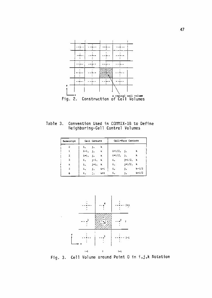
In COMMIX-1B, the control volumes are referred to as computational

cells and are defined by the locations of cell volume faces with grid

points placed in the geometrical centers of the cells. The cells

defined in COMMIX-1B may be nonuniform as shown in Figure 2. In addi-

tion, the neighboring cells and cell faces are defined according to

the convention given in Table 3 and shown in Figure 3. The thermal

Table 1. Variable Values for the Conservation Equations

in Cartesian Coordinates

Equation Variable (,) Direction

DiffusionCoefficient

(r )#

Source Term (SO

Continuity 1 Scalar 0 0

Mbeemtum

(0 u x direction Pgx + Vx Rx (;!)

(ii) v y direction pg + V - R - C.1)y y y DY

(iii) v 2 direction Si "2 + Vs Rs Q!)

Energy h Scaler k ilk + 4rb

+ 4 4.dt

Vs, V y$ Vs Balance of the viscous diffusion terms

Rx, Ry, Rs : Distributed resistances due to solid structures in momentum control volume

OrbRate of hest liberated from solid structures per unit fluid volume

0 : Rate of internal heat generation per unit fluid volume

'4 : Dissipation function

Table 2. Variable Values for the Conservation Equations in Cylindrical Coordinates

Equation Variable (0) Direction

DiffusionCoefficient

(r )

Source Term (4)

Continuity

Mbmentum(1)

(if)

(111)

Energy

I

vr

'13

vr

h

Scalar

r direction

0 direction

z direction

Scalar

0

I:

P

P

k

0

v20 I 3

p --r

+ pgr+ V

r r r 3r- R - - -- (rp)

*apyre°

I a+ pge + ve Re - iii (p)

r

pgz

+ Vz- R -

z 32(p)

12 + 0 + Q +dt

Orb

a : Centrifugal' force tern

A : Coriolis force term

Vr. Ve. Vr : Balance of the viscous diffusion terms

Rr, Rs, lir : Distributed resistance due to solid structures in a momentum control volume

/lrbI Rate of heat liberated from solid structures per unit fluid volume

4 : Rate of internal beet generation per unit fluid volume

: Dissipation function

47

L.Fig. 2.

A typical cell volume

Construction of Cell Volumes

Table 3. Convention Used in COMMIX-1B to DefineNeighboring-Cell Control Volumes

Subscript Cell Centers Cell-Face Centers

0 1, j, k

1 i-1, j, k i-1/2, j, k

2 1+1, j, k 1+1/2, j, k

3 i, J-1, k I, j-1/2, k

4 i, j+1, k i, j+1/2, k

5 i, j, k-1 i, j, k-1/2

6 i, j, k+1 i, j, k+1/2

4

L.3 - - - i-1

i-1

Fig. 3. Cell Volume around Point 0 in i,j,k Notation

48

hydraulic properties of the fluid are calculated at the cell grid

points and are assumed to remain constant over the entire cell.

Since the values of fluid and flow properties are calculated

at the grid points, the following dilema arises. Because the convec-

tive terms in the conservation equations require velocities on the

cell faces, these surface velocities must be obtained as averages

of grid point velocities which are less accurate. Furthermore, since

each of the momentum equations has a pressure derivative in the source

term, a central difference approximation to this pressure term must

span 3 grid points. As a result, the derivative is an average over

two cell lengths and is less accurate. The way in which to reduce

the need for velocity averaging as well as to tighten the pressure

derivative is to stagger the velocity grids so that the velocities

are actually calculated on the cell faces. Since this staggering

places velocity grids between adjacent pressure grids, the required

pressure derivative can be approximated using the values at adjacent

grid points. As a consequence, the central difference pressure ap-

proximation spans only one cell length and is more accurate.

Figure 4 shows the locations of u and v by short arrows on a

two dimensional grid; the three dimensional counterpart can be easily

imagined with respect to a grid point, the u location is displaced

only in the x direction, the v location only in the y direction and

so on. Since the velocity grids are staggered, the control volumes

used for the conservation of momentum are also staggered. From now

on these staggered control volumes will be referred to as momentum

control volumes while the remainder will be referred to as main control

49

roommtumControl Volume

1 I 1

.......... ........

1

.. .r....

1

Fig. 4. Staggered GridV

Other variables

Fig. 5. Momentum Control Volumes

somenttoControl Volume

Table 4. Convention Used in COMMIX-1B to DefineNeighboring Control Volumes for the iDirection Momentum Equation

SubscriptMomentu ControlVolume Centers

Momentum ControlVolume Face Centers

0 1+1/2, j, k

1 1-1/2, j, k 1, J. k

2 1+3/2, j, k 1+1, j, k

3 1+1/2, j -1, k 1+1/2, j -1/2, k

1+1/2, j+1, k 1+1/2, j+1/2, k

5 1+1/2, J, k-1 1+1/2, 3, k-1/2

6 1+1/2, 3, k +1 1+1/2, J. k+1/2

50

volumes. As shown in Figure 5, the control volume for momentum will

be staggered in the direction of the momentum such that the faces

normal to that direction pass through the grid points. The convention

used in COMMIX-1B to define neighboring momentum control volumes is

shown for the i direction momentum equation in Table 4.

3.4 Finite Difference Approximations

Finite difference approximations to (3.2.7) are derived by inte-

grating (3.2.7) over a control volume. The integration of (3.2.7)

will be shown term by term in Cartesian coordinates.

Representation of the term a (ivp0) is obtained by assuming thatat

the values Po and 00 prevail over the entire control volume. Inte-

gration of the unsteady term over the control volume then gives

.)1..

P(3.4.1)-51

4yvpciOd

xdYdz ((pin) -( :

5t '

)n)V"

where Vo = YvAxAyAz is the volume of the fluid; the superscript n

refers to old time-step values, and the superscript n+1 for the new

time-step values is omitted for simplicity. For the x-momentum control

volume the formulation is the same except that the volumes and densi-

ties used are averages of the values existing in the two main control

volumes overlapped by the x momentum control volume. The volume of

the fluid in the x-momentum control volume is given by

(3.4.2) Vo = 1/2 (yVi

+ yVi+1

)1/2 (Axi + AXi4.1) AyAz,

and the density is given by

51

AXipi AXi-FlPi+1(3.4.3) P = Pi+1/2 AXi + AXi+1

In the material that follows a bar over a variable will be used to

denote variables that pertain to momentum control volumes.

The integration of the convection terms over a main control volume

gives

tYxPUO) A(YvPV0)(3.4.4) + "

AX A Azxdydz

= F2<o>9 - F1<06 + F4<4>21 - F3<08 + F6<o>2 - F5<o>8

Here, Fk (=density x velocity x flow area) is the mass flux across

surface k. For example,

(3.4.5) F2 = Fi+1/2 = 9 (ixuA34z)2 = 9 [uAx]2

1+1 (uAx)i+1/2

is the mass flux across the east surface. In this expression

(3.4.6a) <pi = po (if U2 > 0), and

(3.4.6h) <pi = p2 (if u2 < 0).

In general the superscript location is to be used for positive velocity

and the subscript location for negative velocity. In this way the

value of p on the surface is identical to its value at the grid from

which convection is assumed to occur. This means of assigning a property

value is referred to as upwinding since the property value on the

surface is assigned the value that exists at the grid directly upwind

52

from it. Since the values of 0 in (3.4.4) are similarily upwinded,

the term, F2<01, in (3.4.4) may be rewritten as

(3.4.7) F2<0>9 = 10,F210o 10,-F2IO2,

where the quantity 1A,B1 = max (A,B). Using this formulation (3.4.4)

may be rewritten as

(3.4.8)J[1(ykou0) A(Yypv0) 0(yzPw0)1

_ Ax AyAz

dxdydz

= [10, F2I 10, F4I 10, F6I 10, -F1I 10, -F3I 10,-F51]00

- [10,-F2102 + 10,-F4104 + 10,-F6106 + 10,F1101 + 10, F3103

+ 10, F5105].

The convective fluxes for the main control volume are listed in Table

5. For the x-momentum control volume the formulation is the same

except that the pecularities of the control volume force the expressions

for the fluxes to be somewhat different. The convective fluxes for

the x-momentum control volume are listed in Table 6.

The integration of the diffusion terms over a main control volume

gives

(3.4.9)Ji

[IA(ixr04/Dx) A(yyr030/3y) A(Yzr0D0/Dz)jdd dx y z

Ax Y Az

02(o2-4)0) pl(oo-o1) + D4(04-00)

D3(00-03) + D6(06-00) D5(00-05)

= D101 + D202 D303 + D404 + D505 + D606

- (D1A-D2+D3+D4+D5+4)00.

53

Table 5. Convective Fluxes for Main Control Volume

F1

F2

F3 (A v)j-1/2

(A v)Y j+1/2

F5 (Azy)k-1/2

F6 (Az w)k+1/2

 0

0

2

 0

<0>4

0

6

Table 6. Convective Fluxes for x Momentum Control Volume

F1

F2

1

PO 2

1

9 2 2

L(.A)

A

i-1/2

J+1/2

(uAx)i+1/2]

('lAx)i+3/2]

: Po

F4

F5

1 r2

F6

:

2[<9

>0 vAy)i,j-1/2

>4 ( vAy)i,j+1/2

5 r>0 oiAz)i,k-1/2

>6f

wAz)i,k+1/2

+ 2

23 (vAy) 1+1,j-112]

2+ 24 (vAy)i +1,i+1/1

(°7z) i+1,k-1/2]

(Oh'z)i+1,k+1/2]

54

In this equation D is the average diffusion strength across a

surface of the control volume. Its value is obtained by assuming

that a uniform value of diffusivity r(1) prevails over each main control

volume and using harmonic interpolation to obtain the average at the

surface. For example,

-1(3.4.10) D2 =

2r0) 2r2

the expressions for the diffusion strengths are listed in Table 7

for the main control volume. For the x-momentum control volume the

formulation is the same except that the pecularities of the control

volume force the diffusion strengths to be averaged differently.

The diffusion strengths for the x-momentum control volume are listed

in Table 8. (In these expressions a quantity listed as r2k means

the value of r existing in the (i +1)st cell with respect to cell k

about cell 0.)

The finite difference representation of the source term S is

expressed as

(3.4.11) S = Sco + Sp000,

where Sco, Spc, and 00 are assumed to prevail over the main control

volume surrounding point 0. This linearization of the source is very

practical in a finite difference formulation. For example, the gravity

term in the x-momentum equation represents a constant source term

while the frictional drag term depends upon velocity. In (3.4.11)

the coefficient Spq must always be less than or equal to zero; otherwise

instability, divergence or physically unrealistic solutions will result.

The integration of the source term over the control volume gives.

55

Table 7. Diffusion Strengths for Main Control Volume

1

D2

03

4

5

06

(Ax)1 -1/2 [0f)0 * (4211'2)

-1

Ax) 1+1/ 2 [02-;-) (11)21

( Ay) J-1/2 [(tXr) * 0 r)3o

( Ay) j +1/2 No Ur/

( Az) k-1/2 RA2110 (Azr )

1-i(Aditin [CM Gi)6.1

Table 8. Diffusion Strengths for x Momentum Control Volume

3 [(1,2 x

) 1-1/2 ( Az)14.1/ 2 j 16x/

32 2 L A (x- 1.1 /2 A)1+312.1 \ )2

67..1 ay

53 (Ay)1.10-ini ET= 777r 1-1

14 A, 1.j+1/2 (a7)141.i+1/23 r4

Ask_i "k -1DS

; 2 [(Az) 1,6-1 / 2 ( Ad1+1.6-1/ { 1FT; 171.5 17+ 17]

ag,_+.IBA) *(A) .] [ri 1,'=:T rf,;IF]-1

6 2 z 1.1v1.1/2 1+1,1L4.1/2 r6 ' :V

56

(3.4.12) J S4dxdydz = Scolto + Sp01/000

c.v.

for the main control volume. For the x-momentum control volume V0

is simply replaced by Vo.

Having looked at each term of the general equation separately,

it is now possible to assemble all of the terms of (3.4.1), (3.4.8),

(3.4.9), and (3.4.12) for the main control volume to obtain the general

finite difference equation.

1(3.4.13) (unsteady)+(Convection)-(Diffusion)-(Source) dxdydz

. ((f)(00-(P4 )0)vo4' f10,-F1,1+10, F21+.../ Oo

At

(unsteady) (convection)

flO,F11401 + 10,-F214,2+ .../ + (1)11)2+...)00

(Convection) (Diffusion)

- [D1o1 +D2o2 + .. ] - SCOVO Spoolio = 0

(Diffusion) (Source)

Since the values of 00...06 may change over a time step, it makes

sense to use a weighted average of new and old time values of cb in

the convection, diffusion, and source terms. To accomplish this averaging

the values of (f)i used in these terms is replaced by

(3.4.14) Ti = aoi + (1-00in,

57

where a is an implicitness parameter that ranges between 0 and 1.

By making this replacement in (3.4.13) and rearranging the terms so

that only terms containing 00 are on the left hand side, the following

equation is obtained.

(3.4.15) 00 flVt0 + ai(10,-F11+...+10,F61)

+ (D1 +...+ D6) - SpoVon

= a[(10,F11+ D1)01 +...+(10,-F61+4)06]

(1-a)[(1°,F11+1)1)01n+-..÷(1°,461+4)069

Oon (1-a)[(I 0,-F11+.-.+10,F61)+(314"...4)6)-Sp0V0]

(

PnnOn

V0 4. scovo)

(3.4.15) may be re-expressed as

(3.4.16) 400 = a(a101+402+a'iO3+404+405+406

+ blo + go + go

For ease in reading, the coefficients of (3.4.16) are given in Table

9. The equation for the x-momentum control volume is similar except

that the quantities p,V0, F, and D are replaced by f70, Vo, F, and

D. (In table 9 the quantity listed as 4 (2) arises from an alternate

derivation and is irrelevant to the present discussion.)

58

Table 9. General Finite Difference Equation for theMain Control Volume and Its Coefficients

a 0.0 ' a (aia1

a.6 0 0+ (b1# + b? + b?0)

al : (10,011 + D1)

: ( lo,r31 + D3)

4 : (10,F5i

: (10,-021 + D2)

at : (10,-041 + D4)

a6

: (10,-061 + D6)

(1 - a) (at+ + a.? + at.; ++ at4 + at+bl0

b20 - (1 -a) R10,-111 + + 10,r61) + (DI + + D6) - svo] +o

(Pna."--tt:* SalV0

b30

p

at Ia'fll : + [(10,- l I

'(1st fors)

a°0(2) : a (4 + 4 +

(2nd fora)+ (1 -a) (Fi- 1,2 +13 - 74 + 15 - F6)

+ so" + 100,61 + (DI + D2 + 06) Sp, Vo]

at) +(lrE' sp+) vo

59

3.5 Pressure Equation

As seen previously a pressure derivative term appears in the

source term of the momentum equation. However, since the pressure

is unknown, it must be determined from another equation. What is

done in COMMIX-1B is to relate the velocity to pressure in such a

way as to remove the pressure term from the momentum equation. Next,

the pressure velocity relationships are used to replace the velocities

in the continuity equation to yield a pressure equation that is con-

strained to satisfy continuity.

As mentioned previously the x-momentum equation may be written

in the form

(3.5.1) 400 = (a101+....406) + bio+I++bo,

and from table 9 the term 1:$o contains the term Scoll0. Since a pressure

derivative term appears in Sco, (3.5.1) may be rewritten as

(3.5.2) 400 = (401 +...+ aog) + LA° + b o + 1+1OVIDox

where lAol is used to indicate that the pressure term has been removed

from 0o. To remove the pressure term from the equation, 00 is first

written as the sum of pressure independent and pressure dependent

terms

(3.5.3) 00 = 0 - OAP

Next (3.5.3) is substituted into (3.5.2) to yield

(3.5.4) at 6-OAP) = (401+...+406)+blo+qo+bo'- AP 6,11:

60

In order for the pressure to vanish from the equation, it is essential

that the coefficient of proportionality be given by

Go(1/2)(yvicyvi+1)(1/2)(Axi+Axii.1)AyAz

a0Ax a(15(1/2)(Axi+Axi+1)

= (1/2)(Yvi+ivii.1)AyAz/4

Having removed the influence of pressure from the momentum equation,

the momentum equation is used to solve for the pressure independent

contributions to the new time velocities as

(3.5.6)q

((a101+...+ag06) + blo + b o + bp')/at

Continuity is next used to constrain the pressure field. The

continuity equation for a cell about point 0 is derived from (3.4.15)

by substituting 0 = 1 diffusion strength D = 0, and source strength

S = 0.

(3.5.7) Vo(ap/at) - (Axu)i-1/26 + (Axu)i+29

- (Ayv)j-1/28 + (Ayv)ii.1/2<04

- (Azw)k_1/28 + (Azw)0.1/2<04 = 0

To obtain a pressure equation, the following relations are substituted

into (3.5.7).

61

and

(3.5.8) u2 = u2 - d121 (P2-P0);

ul = ul - di (P0-P1);

v4 = v4 - d4 (P4-P0);

v3 = v3 - d3 (P0-P3);

w6 = w6 dg (P6-Po),

w5 = w5 - dg (Po-P5).

By making these substitutions in (3.5.7) the following equation is

obtained

(3.5.9) agPo - i!, Pl - bg

This is the pressure equation that the conjugate gradient method is

used to solve. The coefficients of (3.5.9) are listed in Table 10.

After solving for the new time pressure field, the total velocity

fields are calculated from (3.5.3). From this point the code moves

on to solve the energy equation.

3.6 Mass Rebalancing

The mass rebalancing scheme is a means of accellerating the con-

vergence of the pressure equations by first making large scale correc-

tions to the pressure field so that the linear equation solvers are

required only for fine pressure adjustments. To make these large

scale adjustments many computational cells are first grouped into

N regions as shown in figure 6. To obtain a pressure correction for

each region, the pressure equations of all cells within the region

are added under two constraints. First, the pressure corrections

efikk C;\CP tg\.JahJOk

x

CM

0

C.*

1.1.

1.

-10

x -k4

i9

VI.

CZP

CP#

tPis;\\

\''1,

010',,

4

/..)

x

0\to'

IC:4

L9 1'P

VI.

CI

CP+

4

t.\

"117:

k_X\

x

'R,

\rtP

.1)\41,

4\*

it*Q0'L9-1

C.

fZ

+V

.S..<..k4

-\

,e\\rt°

VI

x

')I,

4'4% 41

itC)J

L9

Di

CZI

to+

CI)-1

1r

4t

.,..4'4

-NI

19

'V')

'Vlo

X\\el*IA) i

1914Z)

x -1/443

krt.

t4

41le

(Z)

1,.

19-1

,N. lr

q)loN.e.-k4

x

%V+

\\e1,

0

42

2.0

L911/43

to41

-1C:1

1 ,,i..);

11/41

L9

x

L9

.1."i

%

tt41

.-.'\V

x\4t

x

-.%sy

,%N.1#

L9 -10n)'

{)`-

x.s*

,IJI

o'V

x

.t°4

`4

VIP

x

'V

s)° Q

r.;.1

$,;*

irk)

i1.

'1,/,0

L91CI

lbAO

x

,*%\%

41

-.41.,-

tot)

Q01,x

63

NI I

I

I I 1

s

1 I_ _ +. _ t_ _ _ _1- - --II I I- I-. -I - - ..1- .... -4-. - + - ..L

I I I I1

.. .. I-- j

_i-r

I - iI

I

I 1----

-- -

-- -,

i

I

n t Iit

I

---4.---i 1

nI I

I 1

1

iI1.,-1

1I

I

I

I

iI I

I--

I I

L 1--1 I,

I

I I__I-- 4-I rI I

1

I I

I 1

1 I 1

--4. + -r

1 I I1

1

I I 1

I I I

I I

I 3 1

1

g

1

f-I

.

I I II

$

I 1

,

1 21

I

I

ri

I

I

I REIGIONiII I .

i

1

1 !

;

I

RebalancingSurface n

Fig. 6. Coarse Mesh Showing Rebalancing Regions

64

for all cells within a region are the same, and, second, the pressure

correction for each region is determined such that the sum of mass

residuals over all cells in that region equals zero.

The regions shown in figure 6 are chosen so that any region n

has neighboring cells contained only in the neighboring regions (n-1)

and (n+1). Mass leaving the region n and entering the region (n+1)

does so through rebalancing surface n. Mass leaving the last region

N goes into the remaining cells where no rebalancing performed. (It

should be noted that in this discussion N refers to the number of

regions not the number of cells. Consequently, N should not be con-

fused with the N used in Chapter 2). Furthermore, region 1 has neigh-

boring cells only in region 2.

To derive the pressure correction let P* be the pressure distri-

bution which does not satisfy the continuity equation. The pressure

equation for a cell m is

(3.6.1) amoP*m -161 am1P1 -bmo = erm,6

1

where 6*m is the mass residual, and am and bm are the pressure equation

coefficients of (3.5.9). Next, the pressure equations for all cells

m in the region n are added to yield:

6(3.6.2) z [amoP*m -1E1 (am1P*1) - bmo] = 6*m

men 1=1 men

If AP1, AP2, ...APN are the pressure corrections for the rebalancing

regions 1 to N, the new pressure distribution can be written as

(3.6.3) Pm = P*m + APn; men

65

If this new pressure field replaces the old one in (3.6.2), the following

equation results for each region.

(3.6.4) 6men (amoPm - E aml P1 bmo) = 6n1

1=1 men

Since the second constraint requires that

(3.6.5) E sm = 0,men

expanding (3.6.4) by (3.6.3) yields,

. 6(3.6.6)

meEn(amoPiii -

11 1

E amiP*-bmo) +=

6APn [E (amo - E aim)] -APn..1[E ( E aml)

men len men len-1

APn+1 kn(ferolami)] = 0, (n = 1,....N).

The first term is simply E d* from (3.6.2).men m

6Furthermore, since amo =1E1 aml, and since aml = aim, many cancellations

=

will occur when the second term is evaluated with the result that

6(3.6.7) (amo - am]) =

men+ (E ami ).

men n leE mn en leE

an-1

men n lentl

As a consequence, (3.6.6) may be rewritten as

where

(3.6.8) AonAPn-Ainon_i A2nApro1 - Ein = 0,

(3.6.9a) All = E (E

aml);men le (n-1)

66

(3.6.9b) 4 = E (Z ami);mcn 1E(n+1)

(3.6.9c) Ag = A7 + 4, and

(3.6.9d) Bn = E 6*m.men

For the first rebalancing region, the coefficients Al = 0, and Ao

A.Al2

Since no pressure is desired in the neighboring cells of the

last rebalancing region, APN+1 = 0, and AZ can be evaluated from (3.9.6b).

(3.6.8) yields N equations for the N rebalancing regions. Since

these equations may be solved using a tridiagonal matrix algorithm,

the large scale pressure corrections are easily obtained. After obtaining

these corrections, the linear equation solvers are used to make fine

pressure adjustments so that mass is conserved on both a cell by cell

and a regional basis.

3.7 Solution Procedures

As mentioned previously COMMIX-1B solves the conservation equa-

tions of momentum, mass, and energy in each outer iteration. Further-

more, it was shown in section 3.4 that the conservation equations

allow values of the dependent variables to be represented as a weighted

average of the old and new timestep values using an implicitness par-

ameter a that ranges between 0 and 1. Although any value of a between

0 and 1 should work, the solution scheme has only been fully tested

for a values of 0 and 1 at the present time. It is therefore recom-

mended that only a values of 0 and 1 be used in the solution scheme.

The solution schemes, resulting from these values of a are shown in

tables 11 and 12 respectively.

67

Table 11. Algorithm of the Semi-Implicit SolutionScheme (a=0)

1. Calculate momentum coefficients using old-time step values of u,v, and w:

d (

2. Calculate pressure equation coefficients using 4, dO:

P Pa

0 ,aP

, b0

.

I

3. Solve pressure equation for new-time pressure Pn+1:

P ra0P0 at

P

PL b0

4. Calculate new-time velocities using

tie ; ($ u,

and new-time values of pressure.

5. Calculate energy equation coefficient using new-time values ofvelocities:

eh, bb0' 0

6. Calculate new-time enthalpy hn+1:

ho a;h2 by /a0 .

68

Table 12. Fully Implicit Solution Sequence (a=1)

1. Calculate velocity-pressure relation coefficients from theprevious iterate values of u, v, and w:

;, d4; (0 - u, v, w).

2. Calculate pressure equation coefficients using ;,

P, atP b0 Pact, .

3. Solve pressure equation for new-time, new-iterate pressure P:

poPo =1 + b;

4. Calculate new-time, new iterate velocities u, v, w from velocity-pressure relations:

=; - oe AP ; (.0 - u, v, v)

5. Calculate energy equation coefficients using new-time, new-iteratevelocities:

h h

a0, ath ' b0

6. Solve energy equation for new-time, new-iterate enthalpy h:

a0 h0 G athht b0

7, Check for convergence of u, v, w, h; if not converged, return toStep 1.

69

CHAPTER 4

COMPARISONS BETWEEN THE S.O.R. AND CONJUGATE GRADIENT METHODS

4.1 Introduction

The comparisons between methods were made for six-steady state

problems run with COMMIX-1B. In all of these cases the mass rebalanc-

ing technique described in Section 3.6 was used to accelerate the

convergence of the pressure equation. In addition, for each outer

iteration the maximum number of internal pressure iterations was lim-

ited only by the default value of 99. This choice was made for two

reasons. First, an unknowledgable user would most probably rely on

default values in the absence of any better information. Second,

this choice allowed the pressure field to converge on most outer itera-

tions with the result that the velocity fields on equivalent outer

iterations were fairly similar. Since the velocity fields obtained

affected the coefficients of the pressure matrix on the next outer

iteration, allowing the pressure field to converge forced both methods

to solve fairly similar systems of equations on each outer iteration.

The over-relaxation factor was set to 1 for the first problem and

1.3 for the second. For the remaining problems this parameter was

set to its default value of 1.5.

In comparing the performance of these methods three topics need

discussion. In section 2 each of the problems run will be sufficiently

described, and the total running times for each solution scheme will

be given. In section 3 the significant differences between solution

schemes will be discussed. These differences will be used in section

70

4 to explain differences in the ratios of running times between the

problems described in section 2. In addition, several questions will

be raised about other factors affecting the problem.

4.2 Problems

The first problem modeled was the flow of liquid sodium through

a canned hexagonal 7 pin fuel assembly. Vertical and horizontal cross

sections of this assembly are shown in figures 7 and 8, respectively.

Fluid entered the assembly at the bottom of figure 7 where it was

forced to have constant temperature and normal velocity values of

553°C and 2.15m/s. Fluid left the assembly at the top of figure 7.

Here the temperature and normal velocity values were initialized to

553°C and Om/s but allowed to vary to satisfy conservation requirements.

In addition the pressure at this surface was assigned a constant value

of 1.32X105 Pa.

Because the fuel assembly is symmetric, only one quarter of the

assembly was modeled as shown in figure 8. As a consequence, the

uppermost and rightmost surfaces in this figure correspond to symmetric

surfaces while the remaining surfaces correspond to the assembly can-

ning. To model these surfaces free slip boundary conditions were

used with the normal velocities on all four surfaces initialized to

0 m/s. No heat transfer was allowed across the surfaces of symmetry

while heat transfer to the canning was allowed. In addition, the

temperatures of these surfaces were initialized to 553°C but allowed

to vary to satisfy conservation requirements.

Although the fuel rods and spacer grids are not shown in these

figures, their influence on the fluid temperature and velocity was

71

Figure 7. Vertical Cross Section of 7-Pin Fuel Assembly

72

Figure 8. Horizontal Cross Section of 7-Pin Fuel Assembly

73

accounted for. The energy transport between these strucutres and

the fluid was determined from heat conduction equations and convective

heat transfer correlations. The influence on the fluid velocity was

determined by taking both the direct resistance and frictional resist-

ance of the structures into account. The direct resistance was deter-

mined by adjusting the volume porosities and directional surface poros-

ities of each cell to make the flow pattern account for the shape

of these structures. The frictional resistance was determined by

the use of friction factor correlations. Because the rods affected

fluid temperatures and velocities, this problem required the solution

of all three conservation equations.

This problem converged in 52 outer iterations for both the conju-

gate gradient method and the S.O.R. method. The total time spent

solving the pressure equation was 6.14s for the conjugate gradient

method and 11.60s for S.O.R.

The second problem involved the flow of water in a scaled model

of the Clinch River Breeder Reactor outlet plenum. A cross-section

of the resulting flow pattern is shown in figure 9. In this figure

fluid enters at two places in the bottom and leaves at the knob on

the left hand surface. The first inlet occurs at the two large cells

in the bottom which are shown with dotted lines. This inlet corresponds

to the reactor coolant coming from the fuel and was assigned constant

temperature and normal velocity values of 81.67°C and .904 m/s. The

second inlet occurs in the cells adjacent to these and corresponds

to the reactor coolant which was diverted to cool the breeding blanket.

This inlet was assigned constant temperature and normal velocity boun-

74

4

a

$

t

t

p

vk

t t, t t. t t. t. t, t ta 't4 tt 1

a

4

4

S

tt t.t tt t.t t ,

$

a

4

4

Figure 9. Vertical Cross Section of C.R.B.R. Outlet Plenum

75

dary conditions of 49.5°C and .179 m/s. The temperature difference

between these two streams required the energy equation to be involved

in the problem solution. The temperature and normal velocity at the

exit were initialized to 81.67°C and 0 m/s but allowed to vary to

satisfy conservation requirements. The pressure at this surface was

assigned a constant value of 98,569.1 Pa.

The upper surface was assigned an initial temperature boundary

condition of 81.67°C but allowed to vary. The centerline was assigned

a free slip velocity boundary condition while the remaining surfaces

were assigned a constant normal velocity value of 0 m/s.

For this problem convergence was obtained in 236 outer iterations

using either solution scheme. The total time spent solving the pres-

sure equation was 32.96s for the conjugate gradient method and 74.06s

for S.O.R. Out of curiosity this problem was tried without mass re-

balancng causing convergence to be obtained in 236 outer iterations

with the conjugate gradient method and 211 iterations with S.O.R.

The total time spent solving the pressure equation was 35.26s for

the conjugate gradient method and 105.26s for S.O.R.

The third problem involved the flow of air through an atmospheric

fluidized bed combustor. Vertical and horizontal cross-sections of

the resulting flow pattern are shown in figure 10 and figure 11 respec-

tively. In this problem air entered the combustor from 3 places.

The first inlet was at the bottom surface which was assigned constant

temperature and normal velocity boundary conditions of 871°C and 2.58

m/s. The second and third inlets were located in the rear most plane

76

4

4

4

4

'4

44

4 4

4

0

4

a

'4

4

4

0

4

f

..... .

f

.........

'4

44

0

4

tf

' 4

' 4

' 4

4

4

4 4

44.4

44 A

41.. V V!

4 4 4 4 4 4 4 4 4 4 4

a

4

4 a

.. . 7 . . .

4 4 4 4 4 g44 A i A 444 4 4 4 441 4 4,4 4 4

. .. . .. . . . .. .. . .4 .. 4 : 4 i 4 41 4 A :A. : 4 7.4 74 , : 4 iI 4 ol :4 4 4 is. 4 : 4 :4: 4

;.:.4 : 4 : 4:& 41.::114;14.11:44 4:4 ,6 4 4 i 4 7 4

: : : : : : . : .4:.....

- . - - , .

A 4 4 4 i4: & :1:18:4:1:1:4:A 4:44 4.444 Iii. 4'4iii &

A 4 4 4 ' i 7-1.11:-V1**I'llrl'!I'74, 471.74 1".. 4' -.4'. "4' - V '41,-1*-1- -.4.

:

4 4 : 4 :A: : :IL: : JA: :A: : 4 A: 4 : :4 . :* A g :

4 :Ai A ill: : :A- : :A: : :A: 4 : 4 :4 4 a'. - -

A 4 '1: A 4:1:8:1:a.,:8:3:4:8:4:* 44.1'6 *11

Figure 10. Vertical Cross Section of Atmospheric Fluidized Bed Combustor

p. .A p. .110

4

A A

A 9a

A

a a a

4

4

aaa

V

aA

p.

p. S

4

a

77

78

of figure 10 so that the flow from these inlets came straight out

of the figure and perpendicular to the upward flow from the bottom.

These two inlets represented ports which were used to inject low tempera-

ture air at high velocity into the combustor. The action of these

ports is shown in the horizontal plane of figure 11. Both of these

ports were assigned constant temperature and normal velocity boundary

conditions of 288°C and 91.44 m/s. The temperature difference between

these ports and the bottom inlet required the energy equation to be

involved in the problem solution.

The air left the combustor at the uppermost surface in figure

10 which was assigned a constant pressure boundary condition of 1.0135x

105 Pa. Although the temperature and normal velocity of this surface

were initialized to 871°C and 0 m/s, they were allowed to vary to

satisfy conservation requirements. The normal velocities of all remain-

ing surfaces were held constant at 0 m/s while their temperatures

were initialized to 871°C but allowed to vary.


using either solution scheme. The total time spent solving the pressure

equation was 253.88s for the conjugate gradient method and 458.35s

for S.O.R.

The fourth problem involved the flow of water in the cold leg

and downcomer of a PWR. The resulting flow pattern is shown in figure

12. In this figure the horizontal portion is the cold leg having

the high pressure injector on the top right and the downcomer on the

left. The two flow inlets for this problem were at the far right

of the cold leg and at the top of the high pressure injector. The

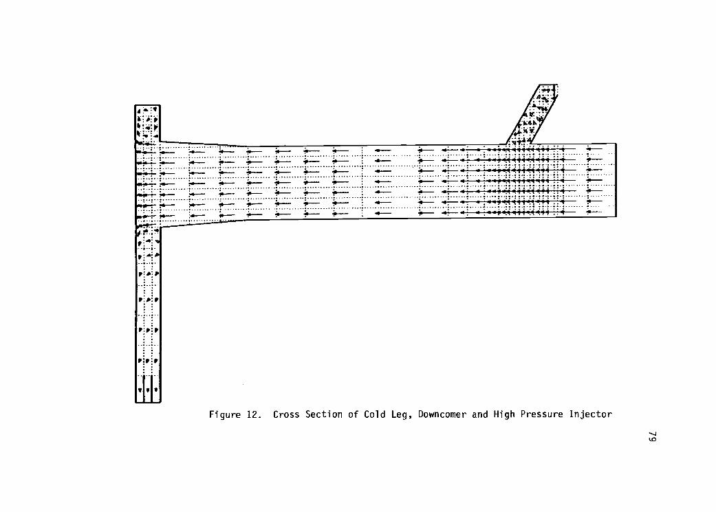
NiIr..4

G)S-=V)r-

1.1-

79

80

first inlet was assigned constant temperature and normal velocity

values of 70°C and .0913 m/s. Since the second inlet was assigned

constant values of 70°C and 0 m/s, it was effectively shut off, and

the fluid in the injector was consequently stagnant. (The arrows

shown in the injector mean nothing because the norms of these velocities

were 4 orders of magnitude below the main velocity in the cold leg,

resulting from the viscous diffusion of momentum.)

The fluid exit was located at the bottom of the downcomer. At

this exit the temperature and normal velocity values were initialized

to 70°C and 0 m/s but allowed to vary after that. The normal velocities

of all other surfaces were held constant at 0 m/s. The temperatures

of these surfaces as well as that of the internal fluid were initialized

to 70°C. Since all temperatures were set at 70°C, no significant

energy calculation needed to be performed.


with the conjugate gradient method and 208 iterations with S.O.R.



The fifth problem involved isothermal air flow through a pipe

having half of its flow area blocked a fifth of the way to the top.

The resulting flow pattern is shown in figure 13. Air entered at

the bottom surface which was assigned constant temperature and normal

velocity values of 25°C and 1 m/s. Air left at the top where these

values were initialized to 25°C and 0 m/s and then allowed to vary.

In addition the pressure at the top was held constant at 7000 Pa.

81

A

t

A

6

4

4

t

f

f

f

6

4

4

a

4

4

f

t

1

t

f

7

7

2

I

I

I

I

1

I

t

7

I

I

7

I

I,

1

1

I

I

1

f

I

I

I

4A

t A

t a

t a

t a

t a

r A

t A

t A

t &

7.

t a

f A

t

f

f A

AA

4 A V

I

I

I

I

4

I

1

4

t 4

t 4

A 4 4 4 4 4 4 A

Figure 13. Cross Section of Isothermal Air Flow through a Pipe

82

The normal velocity at the outside surface of the pipe was held

constant at 0 m/s and the temperature was initialized to 25°C. A

free slip boundary condition was used at the center of the pipe, and

the internal air temperature was initialized to 25°C. Because of

the isothermal conditions at 25°C, no energy calculation was required.

This problem converged in 110 outer iterations using either solu-

tion scheme. The total time spent solving the pressure equation was

21.35s for the conjugate gradient method and 15.60s for S.O.R. Since

the simplicity of the problem geometry made this problem easy to scale,

it was decided to see how decreasing the mesh size in the r and z

directions would influence the running times. The flow patterns for

these cases are shown in figures 14 and 15. For the case shown in

figure 14 the mesh size in these directions was reduced to 2/3 of

that shown in figure 13. This problem converged in 156 outer itera-

tions using the conjugate gradient method and 175 iterations using

S.O.R. The total time spent solving the pressure equation was 71.67s

for the conjugate method and 48.32s for the S.O.R. For the case shown

in figure 15 the mesh size was reduced to half of that shown in figure

13 in the r and z directions. For this problem convergence was ob-

tained in 194 outer iterations using the conjugate gradient method

and 282 iterations using S.O.R. The total time spent solving the

pressure equation was 155.45s for the conjugate gradient method and

117.19s for S.O.R.

The last problem modeled the flow of water in the cold leg and

downcomer of a PWR in which blockage occurred in the downcomer.

The resulting flow pattern is shown in figure 16. In this figure

83

4

4

4

4

...

4 t

4 #

4

4

4

4

4

4

4

4

4

4

t

t

1

t

t

t.t

t

t

t

t

ttt

t.

t-t-tt.

tt.t

4

4

4

4

a

t

4

a

1.

--t t

.t. tt

I tt.tt

1

t t

t t.t t

-t

-t --t

a

4 a

t t

4 a

1...t

t

ft 1 1

1 1 1

t.1 tt'.1 t

"1 t f

1 t t

"t 1 1 f

"1" t 4

't t f

1 1 t 4

"t 1't t

.t. "tt f 4

t t 4 4

# a

# a

a

4

........

4 a

a

a

a

4 a

4 a

4 a

a

4...

a.....

a

a

...a

.....

a

a a

a a

a

a a a

a a V

t t

t f

tt

a

a a

4 a

4

4

a

a

a a


84

aia:1..- %. '1.1.4717T

4..,-7;-.1.4414tAiiieA i :-.

..4.I-.+---4.A444t7tt.t7.t7trfT4.74116.aii4:7r *444".1711.7.1ai.."--747474*AA:7474aA:

--r-";17.47.1I:A:--,74747/11'-=--1-4-44-iltrtti-fttttri::A:ei

4T7474.!.VtiAi-:"-1"47471:T:1:A '-ri7i74iT:A: .--"zri'rcTT1,Ai-"TrTr471:1,

7-747471-14-t"--"4-i'itrl',18 i A i 4- -A-7474rr,:

8A ! : :---rri77-1174:T:1:1:1------rri*'-iit-AH-41.1.i.t.-i-ic441-1-

--ri7a.4.,-;--fit-i.f*tr'ha 1,-41174:1-47

1114.---;Ti4iti-tit-:-ttv4;-4111i/ilti'17'7147470::,..a :

:,--441#17,!1:1-4-44444.17t7rt6:':-7-1-474i:T:

..`.i.-.:+4.7-4.1...4.1...t.i.:.4.t.f..0..4...i..f...i..1.c.41.44.4.4.4....

'----rWr414 A :"""AiA:

8'4:4

: -1.1.tf4:4-..4.7.4.:t.L.A.:4-4.41414j4-47-1:a

. ...:.: .:

71.

: :

: : it41ttftt7f7C71.7i7A4A.;.4.;1-11*

"--A4t

:

'Lf4f41-tttili:f747ii&:,i

tj.A.;-t-1-1-TT :

:Tr4 .... s 1 :7i :

: 444-A4444

iL .14.141ttttf7f7f7i7ikt.14:tit

..11.;.f.1.1.4 ! : :

i f+1.1.,7

T7 I : :

i: : ; .

.- .41-

' ' ;"4";'474-

a a : A :: .

A A-41:4:4::A.A4C41"'.

TIt'l't"1"

:

:

:

-'t 41*: :

,

: :. .. ..: :

4: :

tti-tiltr.474717::iti.i :

4-1

4t4/fif7W74:a:&iai&: :

44-

:

..'.-ra

A

'47174; : i..:.a..

a ; a1.17.4.7.4.74.71

': ...4....;-"

-...,8.......,

: : :.,..,

'....'t414-rt.f7TrITA. .

ti.17.1Tr1.44:17.17.....

. .41,t,f-fra.A.4,t:.titil7r:T7

.87 A '

ft 1 i tt 1 I Si i 7.7 " : ;44' 17:i : : eaf-rt7174;4.&a:a.

,-ttri1747.4"7-47-4-7....,.41.4: 47 4 : 4 : A : a i a

' ri' *I 1 A s A11 4 . ...; A,1.-.1.4:4.7.17."7.i 7 A i a

"..44-4---ri-ri-

-i-t.-1*,-7;: 7 : :

8 i. ii.i..i...i...:;A.

14'441-ir41.A.7.11a. ....;.-4..4";.4..".."f"rfl4A:a

1717174747i1,i,

'CT! 47 4 4 6 !.,4-4-4-1-1-1-1i:A:&:A..:4,.:..


85

..s. re......... ..y. ,,a. -S

....... ..... (..1101e- -.1.-.-s..q.are.-.s.. 0. ..... osi.- ....lb ...

Figure 16. Cross Section of Cold Leg, Downcomer, and HighPressure Injector

86

the horizontal portion is the cold leg having the high pressure in-

jector on the top left and the downcomer to the right. In figure

17 a view of the downcomer in a different plane shows the blockage

which is the cutaway portion near the top of the right surface.

In this problem there were two fluid inlets. The first inlet

was to the far left of the cold leg where the fluid was assigned con-

stant temperature and normal velocity boundary conditons of 64.08°C

and .0161 m/s . The second inlet was on top of the high pressure

injector where the corresponding boundary conditions were 64.08°C

and 0 m/s. Because the normal velocity was set to 0 m/s at this inlet,

the high pressure injector was essentially shut off.

The fluid outlet was located at the bottom of the downcomer.

Although the temperature and normal velocity values were initialized

to 64.08°C and 0 m/s at this outlet, they were allowed to vary to

satisfy conservation requirements. The normal velocities of all other

surfaces were fixed at 0 m/s while their temperatures were initialized

to 64.08°C. The internal fluid temperature was also initialized to

64.08°C. Because the temperatures of all the surfaces and the internal

fluid were set to 64.08°C, the problem was isothermal, and the energy

equation was therefore not required in the problem solution.

Convergence for this problem was obtained in 266 outer iterations

using the conjugate gradient method and 262 iterations using S.O.R.



87

..... .iviiiai4:44:4!!''''ilw V

bib: Iiv;;4.4. : : -4 : 4.4 : ;

: : 0: v: : : : P :

:

.1.....-.`40147VV7*,irerPLZW:.:,;"Atli:V.1E11'94P'

411.0.44-- 4E 4

1ii 1i \ .....

jAii 41+74.144A 4 4

i.,4,0;44 41'4,44 4z4i+tytti

4

4

4 4 4 4

4 4

4

..4.,.

4. 4 \

4

4 4 4 4

4

4 4

Figure 17. Cross Section of Downcomer Showing Blockage

88

The results of all six problems are summarized in table 13.

It should be noticed from this table that the conjugate gradient method

significantly out performed the S.O.R. method in the first four problems

while losing in the fifth and nearly tieing in the sixth. To understand

this behavior it is first necessary to discuss some differences between

the two solution schemes.

4.3 Differences Between Solution Schemes

As can be seen from algorithm 2.9.2, the conjugate gradient method

is executed in three steps. Since step 1 always occurs before the

repetition of step 2, the time taken by this method to solve a system

of equations may be divided into two categories. The first is the

amount of time that is taken to perform step 1 and is fairly constant

for a given problem on each outer iteration. The second category

is the time taken in step 2 which is the product of the time required

for one iteration of step 2 and the number of iterations of step 2.

This result may be expressed mathematically to determine the time

taken by the conjugate gradient method to obtain convergence in one

outer iteration.

(4.3.1) TCtotal = TC1 + TC2NC

For the S.O.R. method, however, there is no initial setup step and

the time needed is therefore directly proportional to the number of

iterations. This may be expressed mathematically as

(4.3.2) TStotal= TSNS

89

Table 13. Summary of Results

#

Problem

Type

# of Cells Total

C.G.

Time(s)

S.O.R.

Time Ratio

(S.O.R./C.G.)

1 German 7 Pin Assembly 432 6.14 11.6 1.89

2a C.R.B.R. Outlet Plenum 346 32.9 74.06 2.25

2b C.R.B.R. Outlet Plenum 346 35.26 105.26 2.99

(no rebalancing)

3 Atmospheric Fluidized Bed 2148 253.88 458.35 1.81

4 Cold Leg and Down Commerof a P.W.R.

978 51.35 103.76 2.02

5a Isothermal Air Pipe Flow 800 21.35 15.60 .73

5b Isothermal Air Pipe Flow 1800 71.67 48.32 .67

(with more cells)

5c Isothermal Air Pipe Flow 3200 155.45 117.19 .75

(with more cells)

6 Cold Leg and Downcommerof a PWR with blockage

3404 207.27 224.56 1.08

90

For the problems run the setup time TC1 in (4.3.1) varied between

2.5 and 4.22 times the iterative S.O.R. time Ts. Furthermore, since

the conjugate gradient method involves more bookkeeping work per itera-

tion than the S.O.R. method, TC2 in (4.3.1) varied between 1.5 and

1.78 times the iterative S.O.R. time. If it is assumed that Ti c =

3TS and TC2 = 1.6Ts, the following crude equation may be derived from

(4.3.1).

(4.3.3) TCtotal 3Ts + 1.6TsNc

By equating (4.3.3) and (4.3.2) a relationship between the numbers

of iterations of the different methods that result in the same total

execution time is obtained.

(4.3.4) 3 + 1.6Nc = Ns.

Equation (4.3.4) has important consequences for the competition

between the methods. When the number of inner iterations is large

for both methods, the setup time becomes negligible and the number

of iterations of the conjugate gradient method must be smaller by

a factor of 1.6 to tie the running time of the S.O.R. method. Obviously

it must be lower by a factor of 3.2 to reduce the running time in

half. When the number of iterations is small the setup time is no

longer negligible, and the conjugate gradient method must beat the

S.O.R. method by greater margins. For example, when Ns=10, Nc I, 4,

and the conjugate gradient method must beat the number of S.O.R. itera-

tions by a factor of 2.5 to tie and by a factor of 5 to reduce the

91

running time in half. Finally, when Ns = 5, Nc q, 1 so that for Ns

< 4 the S.O.R. method becomes unbeatable.

From the previous development it is obvious that the burden placed

on the conjugate gradient method becomes greater as the number of

S.O.R. iterations becomes smaller. Furthermore, when the number

of S.O.R. iterations decreases below 5, the S.O.R. method becomes

unbeatable. As a consequence, the number of inner iterations per

outer iteration must remain high in order for the conjugate gradient

method to remain competitive.

4.4 Summary of Results

The difference in the ratios of running times for different prob-

lems can be explained from the development of the previous section.

In all problems run with the S.O.R. method the number of inner itera-

tions per outer iteration was large in the beginning of a run and

decreased to very low numbers towards the end of a run. As a conse-

quence, the conjugate gradient method beat the S.O.R. method during

the first part of a problem and lost toward the end. It is therefore

obvious that the conjugate gradient method beat the S.O.R. method

by greater than 2 to 1 margins in the beginnings of problems for which

the total S.O.R. execution time was beaten by a factor of 2. On the

other hand, in cases where the total S.O.R. execution time was lower

than that of the conjugate gradient method, the conjugate gradient

method did not beat the S.O.R. method by a large enough margin in

the beginning to compensate for its loss in the end.

The iteration histories that typify these two extreme cases are

shown in figures 18 and 19 which are sketches intended to represent

92

1/11 121 21111

CP/Mt IltRATUNSall

Figure 18. Showing a Typical Iteration History for which theConjugate Gradient Method Beats the S.O.R. Method.

ti 1

- - - CDULGAll INVBIDIr

IME

1E1RATICNOVID ITEI NM 23/1

Figure 19. Showing a Typical Iteration History for which theS.O.R. Method Beats the Conjugate Gradient Method.

93

general trends and not actual cases. Figure 18 illustrates the case

where the conjugate gradient method beats the S.O.R. method by a sig-

nificant margin over a large range and consequently has a lower total

execution time. The opposite case occurs in figure 19 where the number

of S.O.R. iterations rapidly diminishes as a function of the outer

iteration number. In this case the conjugate gradient method beats

the S.O.R. method by only a small margin over a narrow range and conse-

quently has a higher total execution time. The cases where the total

running times are fairly equal are intermediate between these two.

The sketch in figure 18 is tyical of the iteration histories

in the first four problems. Although the decrease in the number of

iterations was not as smooth as shown in figure 18, the common feature

is that the conjugate gradient method beat the S.O.R. method by signi-

ficant margins over long ranges in the beginning of the problems.

The three cases run for problem five had curves similar to those

shown in figure 19. The number of inner iterations per outer iteration

quickly decreased for the S.O.R. method so that the conjugate gradient

method never had a chance to beat it. Throughout most of these prob-

lems the conjugate gradient method converged in fewer iterations than

the S.O.R. method but not sufficiently fewer to reduce the total execu-

tion time.

Problem 6 had iteration curves intermediate between those in

figures 18 and 19. In this problem the conjugate gradient method

beat the S.O.R. method by a significant margin over a moderate range

in the beginning of the run. After this the methods competed rather

equally for a long time, and finally the S.O.R. method beat the conju-

94

gate gradient method at the end of the problem. As a consequence,

the total execution times were fairly equal.

The curves representing the iteration histories of problems 5

and 6 motivate two questions. First, what gives the iteration curves

of these problems their characteristic shapes? Second, since problems

4 and 6 model very similar problems, why should their iteration his-

tories differ so much? One possible explanation for both of these

occurrences is the effect of mass rebalancing. One major difference

between problem 4 and problem 6 is that problem six is divided more

finely into 37 rebalancing regions whereas problem 4 is divided into

only 6 regions. This would imply that the mass rebalancing in problem

6 produces a greater degree of resolution in the pressure field than

that in problem 4. As a consequence, it may be that the pressure

field obtained after mass rebalancing is so close to the iterative

solution that the S.O.R. method converges in few inner iterations,

leaving little room for the conjugate gradient method to beat it.

This hypothesis would also support the rapid convergence obtained

in problems 5a-5c. Since these problems involve linear flow patterns

in the z direction, there is essentially no pressure gradient in the

other directions. Furthermore, since plane by plane rebalancing is

used normal to the direction of flow, the pressure field obtained

after rebalancing is so close to the final solution that the S.O.R.

method converges rapidly, giving the conjugate gradient method no

opportunity to beat it.

This explanation, however, motivates another question. Since

problems 1 and 5 both involve linear flow patterns with plane by plane

95

rebalancing normal to the flow direction, why can the conjugate gradient

method compete in the former problem but not in the latter? Some

minor differences between these problems are that problem 1 involves

a more complicated flow domain with more thermal and momentum interaction

between the structures and the fluid. A more significant difference,

however, is that the over-relaxation factor is 1 for problem 1 and

1.5 for problem 5.

Although mass rebalancing accelerates the convergence of the

pressure equation in some problems, its effects are sometimes peculiar.

For instance, in problem 2, mass rebalancing greatly reduced the execu-

tion time of the S.O.R. method while hardly affecting the execution

time of the conjugate gradient method. There are, however, other

problems in which mass rebalancing greatly reduces the execution time

of the conjugate gradient method. (These problems, however, were

not mentioned previously since no data was taken for them.) This

behavior motivates the following question. What factors contribute

to the difference between solution methods in their sensitivity toward

mass rebalancing?

One of the potential factors affecting the sensitivity to re-

balancing is how the rebalancing regions match the problem geometry

and flow field. For example, plane by plane rebalancing in the z direc-

tion would be inapprpriate for a problem in which the flow was normal

to the x direction. In addition, a rebalancing scheme may be damaging

when it attempts to subdivide regions in which the flow is circular.

For example, if plane by plane rebalancing in the z direction were

used in problem 2, the flow would go up through the center of a re-

96

balancing region and down through the sides of it. This situation

would imply that the pressure gradient is negative in the center of

the regions and positive on the sides. Under such circumstances two

possible situations may occur. First, it might happen that the pres-

sures in the center of the region need to be adjusted downward while

those on the side need to be adjusted upward. Since the mass rebalanc-

ing scheme would apply the same pressure correction throughout each

region, the pressures of all cells within a region would be adjusted

in one direction so that the pressure field may be farther from con-

vergence. On the other hand, it may be that the pressures in the

center need a slight downward adjustment while those on the sides

need a drastic downward adjustment. The effect of the uniform pressure

change in the region may be a compromised solution that significantly

overshoots the required central adjustments and undershoots the re-

quired peripheral adjustments. As a consequence, mass rebalancing

may be ineffective under some circumstances. Furthermore, the inter-

play of the rebalancing regions and the problem geometry may favor

one solution scheme more than the other.

Another potential factor affecting the sensitivity to rebalancing

is the number of rebalancing regions into which the flow field is

divided. As seen previously, finer divisions give a greater resolution

of the adjusted pressure field after rebalancing. Depending upon

whether or not the geometric effects of rebalancing are favorable

to the given problem, the greater resolution may favor or damage one

method more than the other.

97

Another possibility is that the differences in the methods them-

selves may make one method more sensitive to rebalancing. One dif-

ference between the two methods is that for the conjugate gradient

method the pressures are updated in terms of quantities calculated

from the values on the previous iteration. For S.O.R., however, the

pressure is adjusted cell by cell so that the adjustments are made

in terms of both the new and old iterate fields. Whatever the reason

is, it remains clear that for some problems there is a difference

in the sensitivity of different solution schemes to mass rebalancing.

This effect should be investigated.

In the light of the previous discussion, it seems that for pro-

blems like 5a-5c, mass rebalancing is sufficient to obtain rapid con-

vergence, and that combining the conjugate gradient method with mass

rebalancing is essentially "overkill." For other cases like problems

1-4, convergence is still fairly time consuming after rebalancing

so that the conjugate gradient method may be effectively applied.

Furthermore, it was discussed that under certain circumstances the

problem geometry may make the mass rebalancing scheme ineffective

or even detrimental. Since the trend in fluid mechanics codes is

to move toward larger problems for which convergence is slower and

toward more complicated geometries for which mass rebalancing may

be ineffective, the conjugate gradient method has merit as a linear

equation solver.

98

Bibliography

1. Anton, Howard. Elementary Linear Algebra. John Wiley and Sons,New York, 1981.

2. Chandra, R. Conjugate Gradient Methods for Partial DifferentialEquations, Ph.D. Thesis, Yale University, May 1978.

3. COMMIX-1B: A Three-dimensional Transient Single-phase ComputerProgram for Thermal Hydraulic Analysis of Single and MulticomponentSystems. W.T. Sha, H.M. Domanus, et al., ANL-85-42, NUREG/CR-4348,September 1985.

4. Daniel, J.W. The Approximate Minimization of Functionals.Prenctice-Hall, 1971.

5. Engeli, H., T. Ginssburg, H. Ruthishauser, and E. Stiefel. Re-

fined iterative methods for computation of the solution and theeigenvalues of self-adjoint boundary value problems. Mitteilungen

aus dem Institute fur Angewandte Mathematik: 8, Birkhauser Verlag,

Basel, Stuttgart, 1959.

application of the conjugate gradient method to the commix

Documents