Technische Universitat WienInstitut fur Nacrichtentechnik und Hochfrequenztecnik

Universidad de ZaragozaCentro Politecnico Superior

MASTER THESIS

Application of SI frames for H.264/AVC

Video Streaming over UMTS Networks

by

Juan Tajahuerce Sanz

Supervisor: Univ. Prof. Dr. Markus Rupp, Luca Superiori, Wolfgang Karner

Vienna, 20th June 2008

Abstract

In mobile video applications, frames can be encoded using temporal dependencies(to other frames) or spatial dependencies (to the same frame) to reduce the bitrate.Frames with temporal dependencies are more commonly used because of their smallersize, however, in case of error in transmition, it propagates troughout the followingframes.

H.264/AVC defines two new frames, SP (with temporal dependencies) and SI (withspatial), and both of them are interchangeable if an error occurs, stopping its propa-gation.

This work shows the influence of the two quantization parameters of SP and SIframes (SPQP and PQP) on its size and quality, obtaining a conclusion of which valuesuse depending on the probability of switching.

Moreover, this project presents the implementation of the switching process de-pending on the error information obtained from the UMTS network. The error infor-mation is detected by the Mobile Station and sent back through a feedback channelwith a certain delay. The effect of the error and the delay is simulated in order toevaluate different situations.

The switching process is implemented in a Matlab program. Simulations show asave in the bitrate without decreasing the quality with respect not to use SP and SIframes in case of a low probability of switching and with a small delay in the feedbackchannel.

Contents

1 Introduction 1

2 H.264/AVC 32.1 Origing of a new standard . . . . . . . . . . . . . . . . . . . . . . . . . . 32.2 General Features . . . . . . . . . . . . . . . . . . . . . . . . . . . . . . . 42.3 NAL . . . . . . . . . . . . . . . . . . . . . . . . . . . . . . . . . . . . . . 62.4 VLC . . . . . . . . . . . . . . . . . . . . . . . . . . . . . . . . . . . . . . 7

2.4.1 Pictures, slices and macroblockes . . . . . . . . . . . . . . . . . . 72.4.2 Intra-Frame prediction . . . . . . . . . . . . . . . . . . . . . . . . 92.4.3 Inter-Frame prediction . . . . . . . . . . . . . . . . . . . . . . . . 102.4.4 Transform, quantization and entropy coding . . . . . . . . . . . . 11

3 SP and SI frames 133.1 Motivation . . . . . . . . . . . . . . . . . . . . . . . . . . . . . . . . . . 133.2 Applications . . . . . . . . . . . . . . . . . . . . . . . . . . . . . . . . . . 16

3.2.1 Bitstream switching . . . . . . . . . . . . . . . . . . . . . . . . . 163.2.2 Splicing and Random Access . . . . . . . . . . . . . . . . . . . . 173.2.3 Error Recovery and Error Resilinecy . . . . . . . . . . . . . . . . 183.2.4 Video Redundancy Coding . . . . . . . . . . . . . . . . . . . . . 19

3.3 The SP and SI design . . . . . . . . . . . . . . . . . . . . . . . . . . . . 193.3.1 Encoding and decoding process in primary SP frames . . . . . . 203.3.2 Encoding and decoding process for secondary SP and SI frames . 21

3.4 Study of the influence of the different quantization parameters . . . . . 233.4.1 Influence of QP parameter . . . . . . . . . . . . . . . . . . . . . . 243.4.2 Influence of PQP parameter . . . . . . . . . . . . . . . . . . . . . 263.4.3 Influence of SPQP parameter . . . . . . . . . . . . . . . . . . . . 27

3.5 Description of the optimized values for SPQP and PQP . . . . . . . . . 33

4 Modifications in the encoder 35

5 Implementation of the switching process 395.1 General scheme . . . . . . . . . . . . . . . . . . . . . . . . . . . . . . . . 39

5.1.1 UMTS. General transmision scheme . . . . . . . . . . . . . . . . 405.1.2 Location of the Switching program in the UMTS network . . . . 43

5.2 Program performance . . . . . . . . . . . . . . . . . . . . . . . . . . . . 455.2.1 Overview . . . . . . . . . . . . . . . . . . . . . . . . . . . . . . . 45

i

5.2.2 Extraction of the RTP packets . . . . . . . . . . . . . . . . . . . 475.2.3 Switching main routines . . . . . . . . . . . . . . . . . . . . . . . 495.2.4 Error simulation . . . . . . . . . . . . . . . . . . . . . . . . . . . 525.2.5 Delay simulation . . . . . . . . . . . . . . . . . . . . . . . . . . . 55

6 Simulation results 586.1 Simulation overview . . . . . . . . . . . . . . . . . . . . . . . . . . . . . 586.2 Encoding step . . . . . . . . . . . . . . . . . . . . . . . . . . . . . . . . . 616.3 The effect of the feedback channel delay . . . . . . . . . . . . . . . . . . 636.4 Performance Analyisis . . . . . . . . . . . . . . . . . . . . . . . . . . . . 67

7 Final Comments 757.1 Conclusions of the simulation results . . . . . . . . . . . . . . . . . . . . 757.2 Summary of the project execution . . . . . . . . . . . . . . . . . . . . . 787.3 Problems found and future challenges . . . . . . . . . . . . . . . . . . . 79

Bibliography 81

APPENDIX A: Optimization of PQP and SPQP values 83

APPENDIX B: Quantization parameter analysis 86

APPENDIX C: Switching Process analysis 98

APPENDIX D: Encoder’s configuration file 109

APPENDIX E: Decoder’s configuration file 119

ii

Chapter 1

Introduction

The great growth of multimedia applications for mobiles in the last years has obligedto investigate in order to enhace the rate-distortion efficiency without increasing dra-matically the complexity of the systems [1]. In video applications, this enhacementhas been obtained by improving the existing codecs, adding new features. Temporaldependencies (to other frames) or spatial dependencies (to the same frame) are utilizedto reduce bitrate. Temporal dependencies are more commonly used with this purposebecause of their smaller size. However, in case of an error in transmition, it propagatestroughout the following frames while decoding. Thus frames with spatial dependenciesare sent regularly to recover good quality in these cases.

Figure 1.1: Network diagram

In this project, CIF (352x288 pixels resolution) and QCIF (176x144 pixels resolu-tion) videos are encoded with the H.264/AVC codec [2] and transmitted over a UMTSnetwork. H.264/AVC contains two new frame types, SP (with temporal dependencies)and SI (with spatial dependencies). The main difference with the previously existingframes is that SP and SI are interchangeable in case of having an error in the link,stopping error propagation when decoding [3].

This work studies the influence of the two quantitation parameters of SP and SIframes (SPQP and PQP) on its size and quality, and tries to understand the close

1

relation between these values and the probability of swtiching.Part of this project consists of implementing the switching process as a completely

independent program from the encoder. Therefore, two bitstreams, one with SP andthe other with SI frames inserted, are encoded in the transmitter in order to facilitatethe switching. The (switching is carried out depending on the error information ob-tained from the UMTS network (Figure 1.1). The Mobile Station detects the error,which occurs normally in the wireless link, transmitting this information through afeedback channel with a certain delay. Video applications make use of UDP protocoland consequently no retransmission is possible, receiving erroneous packets in recep-tion in case of any transmission failure. This system aborts a sure error propagation inthe decoder produced by the usage of temporal dependences. However the propagationof this error in the decoder is avoided with this system.

The effect of the error and the delay are simulated to evaluate different situations,and together with the switching process are implemented in a Matlab program. Simula-tions show a bitrate saving without decreasing the quality with regard not to use SPand SI frames in case of a low probability of switching and with a small delay in thefeedback channel.

2

Chapter 2

H.264/AVC

H.264/AVC is the newest video coding Standard resulted from the cooperation ofthe ITU-T Video Coding Experts Group (VCEG) and the ISO/IEC Moving PictureExperts Group (MPEG) in a common project known as the Joint Video Team (JVT)[4] [5]. The aim of this project is to enhace the rate-distorition efficiency increasing thecompression and the objective and subjective quality of the encoded video comparedto previous standards (MPEG-2, MPEG-4, H.263) without increasing dramatically thecomplexity.

H.264/AVC is designed to work with different types of networks and to support awide range of applications (video telephony, storage, broadcast or streaming).

2.1 Origing of a new standard

The MPEG-2 video coding standard was developed about fifteen years ago as anextension of MPEG-1, supporting interlaced video coding and at those days this tech-nology was enable to distribute digital TV over satellite (DVB-S), cable (DVB-C) andterrestrial (DVB-T) platforms for transmision of standard definition (SD) and highdefinitions [6].

However, nowadays the number of services offered has increased and also the de-mand of high definition TV. Moreover, new transmision media like xDSL, Cable Mo-dem or UMTS offer much smaller data rates and thus a more efficient data compresionhas been required. During the development of the different standards, continued ef-forts have been made to deal with the diversification of the network types and thereforetheir formatting and robustness needs.

In 1998 the Video Coding Experts Group (VCEG - ITU-T SG16 Q.6) started aproject called H.264L, with the aim of double the coding efficiency of the existing videocoding standard at that moment. In 2001 VCEG and the Moving Pictures ExpertGroup (MPEG - ISO/IEC JTC 1/SC 29/WG 11) formed the Joint Video Team, withthe target to finalize the new video coding standard H.264/AVC.

3

2.2 General Features

All the standards from ITU-T and ISO/IEC JTC1, and also H.264/AVC follows theblock-based hybrid video coding approach, consisting in dividing the picture in macro-blocks, informing about luma and chroma. H.264/AVC compresses the transmitteddata by exploiting temporal and spatial dependencies, using inter-picture prediction(temporal) and intra-picture prediction (spatial).

The extensions to the original standard developed by the JVT are known as theFidelity Range Extensions (FRExt). Some of the new features supported by theseextensions are: higher-resolution color information, increased sample bit depth pre-cision, adaptive switching between 4x4 and 8x8 integer transforms, encoder-specifiedperceptual-based quantization weighting matrices, efficient inter-picture lossless cod-ing, and support of additional color spaces.

The standard allows to use different sets of coding tools, known as profiles [1],depending on the application searched:

Five new profiles are supported in recent extensions and they are used for profes-sional applications and high definition video (HD). The profile used in this work is theextended profile (Figure 2.1). Eventhough it is not recomended for mobile applicationsbecause of its computational complexity, it is the only one that allows working withSP and SI frames.

• Baseline Profile: For low-cost applications with limited computing resources,specially used in video conferencing and mobile applications. All features of

Figure 2.1: Utilities for H.264/AVC profiles

4

H.264/AVC are supported except B, SP and SI slices, weighted prediction,CABAC, field coding and macroblock adaptive switching between frame andfield coding.

• Main Profile: Used for broadcast and storage applications, is the mainstreamconsumer profile. It does not support the FMO feature.

• Baseline Profile: Intended as the streaming video profile, this profile has rela-tively high compression capability and some extra tricks for robustness to datalosses and server stream switching.

As all the previous cases of the ITU-T and ISO/IEC, only the decoder is standard-ized, producing similar output for an encoded bitstream in its input that conforms theconstraints of the standard on bitstream and syntax. This point has its advantages,as for instance the freedom to optimize the different applications; however it does notguarantee an end-to-end reproduction quality.

The video to be codified in a raw format is the input of the encoder (Figure 2.2).The encoded sequence is the output of the encoder to be transmitted. It is also possibleto see the effect that the encoding and decoding process have in the quality of the videosince the reconstructed video is also obtained in the encoder. This outputs representsthe received and decoded video in case of no errors in transmission. Another outputis the trace file, which explains deeply the encoded sequence obtained.

Figure 2.2: Encoder inputs and outputs

The H.264/AVC design is divided into two parts, the Video Coding Layer (VLC),which represents the video content, and the Network Abstraction Layer (NAL), whichprovides a format to the VLC and describes the headers added, depending on thestorage media or the transport layers used.

5

2.3 NAL

The NAL describes the packetization process of the encoded video (VLC) and is de-signed to enable simple and effective mapping to differernt transport layers as RTP/IP,H.32X and MPEG-2 systems for broadcasting services. A description of the differentconcepts of the NAL is given below.

The encoded video is organized into packets called NAL Units, divided into apayload and a header. The header is the first byte of the packet and informs aboutthe type of data inserted in the payload. The structure definition of the NAL Unitspecifies the format for packet-oriented or bitstream-oriented transport packets. Anumber of NAL Units forms a NAL unit stream.

In case of using a byte-stream format, three bytes prefixe every NAL unit to defineits boundaries and also some alignemt data is possible to be added if the system doesnot provide it. In case of using a Packte-Transport System, the boundaries of NALunits are withing the packets.

There are two types of NAL Units, VCL and non-VCL NAL Units. VCL NALUnits represent the values of the different samples of the encoded video, and non-VCLNAL Units contains supplemental information to enhace the whole process like timinginformation and also the parameters sets.

The parameters sets are a group of information useful for a number of NAL Units.Since this information rarely change [6], there is no need to send it with every NALUnit, saving bitrate. There are two types :

• Sequence parameter sets: Information valid for several consecutive codedvideo pictures called a coded video sequence.

• Picture parameter sets: Information valid for one or more individual picturewithin a coded video sequence.

Every VCL NAL Unit has an identifier to refer to a picture parameter set andeach Picture parameter set has another identifier to refer to a Sequence parameter set.Sequence and Picture parameter sets are sent before the VCL NAL Units to whichthey refer. Depending on the application, these parameters are sent withing the samechannel than the VLC NAL Units or through a more reliable transport channel.

All the NAL Units of a encoded picture compose forms an Access Unit. It mayalso contain an Access Unit delimiter and some additional information. In the AccessUnit, the VCL NAL Units contained, are known as the Primary Coded Picture. Anend of sequence NAL Unit is sent if the coded picture is the last picture of a videosequence and an end of stream NAL Unit if the stream is ending.

A coded video sequence is a group of Access Unit with only one Sequence parameterset which can be decoded independently. At the begining of the Coded Video Sequence,an instantaneous decoding refresh (IDR) Access Unit is sent. An IDR is an intra picturethat can be decoded without refering to any picture, and prohibits next Access Unitrefer to previous pictures. A NAL Unit stream may contain more than one CodedVideo Sequence (Figure 2.3).

6

Figure 2.3: Packetization process

2.4 VLC

2.4.1 Pictures, slices and macroblockes

The VCL represents the video data and, as in all prior standards, follows the hybridvideo coding approach. A coded picture is divided into samples of croma and lumacalled macroblocks. The final improvement depends on a big number of small stepsrather than on a single coding element.

A coded picture contains two interleaved fields, one with the odd-numbered rowsand the other with the eve-numbered. In case the two fields are captured in dif-ferent times, the frame is known as an interlaced frame, otherwise it is a progressiveframe. Chroma and luma information is extracted from the picture because humansperceive an scene in terms of brightness and color with greater sensibility to brightness.H.264/AVC separates a color representation into three components, Y, Cb and Cr. Yis luma and represents brigthness and Cb and Cr is the deviation of the color from graytoward blue and red, respectively. Chroma has one fourth of the luma samples (half ofthe number of samples in the horizontal dimension and the other half in the verticaldimension) because of the less sensitivity to color and thats called 4:2:0 sampling with8 bits of precision per sample.

A picture is divided into samples and these are grouped into macroblocks. Lumamacroblocks correspond to 16x16 samples of a rectangular part of the picture andthe two chroma components of a picture are divided into macroblocks of 8x8 samples.Macroblocks are the basic buiding blocks of the standard.

A picture can be divided into slices. Slices are sequences of macroblocks whichcan be decoded independently from other slices even though they belong to the same

7

Figure 2.4: Subdivision of a picture into slices.

picture. The transmission order of macroblocks in the bitstream depends on the Macro-block Allocation Map. FMO is a feature of H.264/AVC which allows the division of apicture into slices depending on the content of the image (Figure 2.4). This concept iscalled slice groups. The specifications of the slices are defined in the Picture parametersset and in the slice headers. Each macroblock have a slice group identification numberto inform to which slice it belongs. In this work FMO is not used and macroblocksare allocated in the slices in raster order.

Five different types of slice-coding [6]are supported by H.264/AVC:

• I slice: All macroblocks from the are encoded using intra prediction, what meansthat do not refer to other pictures.

• P slice: Macroblocks from the slice can be encoded as intra but also using interprediction, refering to other pictures, with at most one motion-compensatedprediction signal per prediction block.

• B slice: All coding types of a P slice are allowed and also biprediction, usinginter prediction with two motion-compensated prediction signals per predictionblock.

• SP slice: Similar to a P slice but allows to be switched by an SI frame.

• SI slice: Similar to an I slice but allows an exact mach with an SP frame forrandom access and error recoery applications.

The last two types of slice have been introduced by H.264/AVC. As a generalscheme, all macroblocks are predicted spatially or temporally, calculating its residual.This residual is subdivided into smaller blocks of 4x4 and these blocks are transformed.The coefficients resulting of this transformation are quantized and encoded using en-tropy coding methods.

8

2.4.2 Intra-Frame prediction

In blocks or macroblocks encoded using intra modes, the predicted block is formedbased on previously encoded and reconstructed blocks from the same picture [7]. Thereare three intra coding types, Intra 4x4, Intra 16x16 and I PCM, and all of them arepermitted by any slice-coding type. Using Intra 4x4 means dividing a macroblock in16 blocks to carry out the prediction. Due to the small size of these macroblocks thereis a more accurate prediction, perfect for those parts of the picture that wants to beencoded in detail. Since macroblocks for prediction of Intra 16x16 type are bigger,they are used to predict smoth areas of the picture. Finally, the I PCM coding typetransmits directly the values of the encoded process.

Intra prediction uses spatial dependencies, what implies the usage of neighboringsamples already encoded for prediction. A constraint intra coding mode can be ac-tivated to allow prediction only from intra macroblocks of the same slice, avoidingpropagation of errors from motion compatation.

Intra 4x4 type permits for each 4x4 block one out of nine prediction modes, DCmode and eight directional modes. In DC prediction, the predicted value is obtainedby an average of the adjacent samples. In directional modes the values of the blocksselected by the direction are directly copied. The directional values are horizontal,vertical and diagonal and they are suited to predict textures with structures in thespecified direction.

Intra 16x16 only allows 4 prediction modes, DC, vertical, horizontal and planeprediction. Luma samples can make use of both Intra 4x4 and Intra 16x16 type whilechroma samples are predicted using Intra 16x16 since chroma is usually smooth overlarge areas. Intra prediction mantains slices independent from others because theprediction is not used across slice boundaries (Figure 2.5).

Figure 2.5: Intra Prediction

9

2.4.3 Inter-Frame prediction

Inter prediction uses previosly encoded video frames to create a prediction model [8].Predictive or motion-compensated coding types are known as P macroblock types.They specify the subdivision of the macroblock into blocks of different number ofsamples. The partitions of luma macroblocks supported are of 16x16,16x8,8x16 and8x8 samples. In case of choosing a partition of 8x8 sample, the standard allows anadditional partition in blocks of 8x4, 4x8 or 4x4 and this information is also transmittedby adding some syntax elements. The partition of the 8x8 partitions is also avalaiblefor chroma samples.

The predicted macroblock is obtained by displacing an area of a reference pic-ture. The dispacement is called motion vector and that is what is transmitted. Themaximum number of motion vectors transmitted for a macroblock is 16, case of amacroblock divided into 4 8x8 partitions and each of them divided also into 4 4x4partitions.

The values of luma and chroma samples are finite, and they represent the values ofcertain points of the pictures. Not only these values can be selected as a reference formotion compensation, but also the values in between. The acuracy of the system is aquarter of the distance in case of luma samples. In case the reference value correspondsto an integer-sample position, this value is copied to the predicted signal, but in othercases these values do not exist. Therefore they are calculated using interpolation. Forvalues at half-sample positions, the prediction is obtained by applying one-dimensional6-tap FIR filter horizontally and vertically. Values at quarter-sample positions arecalculated by averaging samples at integer- and half-sample positions.

Bilinear interpolations are used to obtain the predicted values for the chroma com-ponent, and because of its lower resolution, the accuracy is of one-eight sample position.

This accuracity on motion prediction is one of the most important improvements

Figure 2.6: Inter Prediction

10

added by this standard since it allows a more precise motion representation and alsoa more flexible filtering in prediction.

In case the motion vector points outside the image area, the edge samples aretaken as reference. However, samples from other slices can not be used as referencefor motion-compensated prediction.

Once motion vectors of a picture are calculated, they are predicted using spatialprediction from neighboring motion vectors in a simmilar way intra macroblocks do.With the original motion vector and its prediction, a residual is calculated.

In H.264/AVC more than a picture can be used as a reference. That is known asmultipicture motion-compensated prediction and requires a buffer to store all previousreference pictures in both, the encoder and the decoder (Figure 2.6). Every blockfrom a macroblock transmits a reference index to indicate the position of the referencepicture for this block in the multipicture buffer. Smaller regions than 8x8 share thesame reference index.

Finally, another type called P-Skip is defined to represent large areas with nochange or constant motion with very few bits. This type is similar to a P 16x16macroblock type with the motion vector referred to the picture located at index 0 inthe multipicture buffer.

2.4.4 Transform, quantization and entropy coding

After obtaining the residual information, it is transformed as in previous standards[9]. However, in H.264/AVC the transformation is done by separable integer valuesinstead of a 4x4 distrete cosine transform (DCT). Since the transformation values areinteger, no mismatches while decoding are introdoced. At the encoder the processincludes a forward transform, zig-zag scanning, scaling, rounding and entropy coding.At the decoder the process is the inverse except for rounding. In chroma Intra 16x16prediction mode, DC coefficients are transformed again as well as DC coefficients of thefour 4x4 blocks of the chroma component. Cases of using a second transformation areutilized in very smooth areas because in that situation the reconstruction accuracy isproportional to the inverse of the one-dimensional size of the transform. But there aremore reasons for using smaller size transforms. The first one is that as in H.264/AVCthe predicted image is less correlated, transformation has less improvement to offerconcerning decorrelation. Tranformation increase the noise in the edges of the image,and with smaller transforms it is reduced. Moreover the smaller the transform, theless comptations are required.

After transformation, the coefficients obtained are quantized. The quantizationparameter used can take 52 values and the reduction of bitrate increases with itsvalue. However, this relation is not linear. All quantized transform coefficients ofa block are scanned in a zig-zag fashion but the 2x2 DC coefficients of the chromacomponents, which use a raster-scan order.

Before being transmitted, entropy coding is applied. Above the slice layer, syntaxelements are encoded as fixed- or variable-length binary codes [10]. At the slice layeror below two entropy coding methods are supported by H.264/AVC. One of this meth-ods consists of using a single infinite-extent codeword table for all syntax elementsexcept the quantized transform coefficients. This table is an exp-Golomb code with

11

simple properties. The mapping to this table depends on data statistics. Quantizedtransform coefficients use the scheme called Context-Adaptive Variable Length Cod-ing (CAVLC). In CAVLC, the different VLC tables are switched depending on theconditioned statistics, improving coding performance.

The other entropy coding method is the Context-Adaptive Binary Aithmetic Cod-ing (CABAC). This method improves the efficiency because it uses adaptative codesto the statistics of the symbols. In this project, CAVLC is used. The whole codingprocess is shown in (Figure 2.7) [1].

Figure 2.7: Basic encoding process for a macroblock

12

Chapter 3

SP and SI frames

3.1 Motivation

The new video coding standard, H.264/AVC, exploits in its extended profile the useof two new frame types, SI and SP. SP and SI picture coding was first introduced byKarczewics and Kurceren [11]. They have been created to try to avoid error propa-gation while decoding. Eventhough this was already possible in previous standardswith the existing frame types and other techniques, they may fail to completely stopor effectively reduce error propagation and some of them may not be suitable for videostreaming applications [12].

The most common frame type used and already existing in previous standard, isthe P frame which exploits temporal prediction, that means that previous picturesare referenced to calculate the actual value. This method reduce significativaly thebitrate. However, in case of an error in transmision on a previously recieved picture,the decoded image with the not appropiate values will be stored in the decoder bufferand this frame will be an erroneous reference for next pictures. If only P frames aresent, this error will propagate without any stop, resulting a not desirable situation forthe application users.

This error propagation can be solved by using I frames in H.264/AVC and alsoin previous versions. They exploit spatial prediction, that means that they dependon previously encoded macroblocks from the same frame, but not on previous frames.Thus in case of an error, the erroneous frames will not be referenced if the decodedframe is an I frame.

The reason why not all the frames sent are I frames is that its size is much biggerthan the size of a P frame for a comparable quality as it is shown in Figure 3.1 andFigure 3.2. This is because the correlation among consecutive pictures is higher thanthe correlation among different parts of a same picture. These two pictures representsForeman video with a QCIF resolution and size and quality are depicted for differentvalues of the quantization parameter. The bigger the quantization parameter, the lessbits are sent and the worst quality is obtained.

As a compromise some P frames are sent between two I frames, and the set offrames from an I frame up to the P frame preceding the next I frame is definded asGroup of Pictures (GOP). The smaller the GOP, the more prepared is the transmision

13

Figure 3.1: Comparison of size of I and P frames

Figure 3.2: Comparison of quality of I and P frames

to an error in propagation but also the more bits are sent. In this project, a picturebuffer of one frame has been used, what means the decoder uses only the previousframe for inter-prediction. Thus sending one I frame cuts the temporal referencingand it is equivalent to clearing the buffer.

The two new frame types of H.264/AVC standard, SI and SP, make also use ofspatial and temporal prediction respectively. Thus SI frames are perfect to be appliedto switch between different video sequence [13]. The difference with the previouslycommented method is that SP and SI are interchangeable, that means that both ofthem are able to reconstruct the same decoded picture. In case of a no error situation,SP frames are sent, and only if an error occurs, an SI frame is transmitted.

SI frames are able to stop error propagation as I frames do. No previously recievedpictures are referenced in the decoding process, only previously decoded macroblocksfrom the same frame because of using spatial prediction. This can lead to believe inthe benefits of sending always SI frames. However, as it is depicted in Figure 3.3, itssize is much bigger than the size of an SP frame. This is similar to the comparison of Iand P frames using spatial and temporal prediction respectively. The main differenceis that SP and SI frames obtain exactly the same reconstructed image in the decodingprocess as it has been mentioned before.

In that case it is possible to think about the idea of transmiting always SP frames.In that situation and if a notification of an error is received, an SI frame can be sentinstantaneously. The reason is that an SI can only be transmitted instead of an SP

14

frame and never instead of a P frame. A look in the referenced figure shows that thesize of an SP frame is even smaller than the size of a P frame. However, the graphthat depicts the quality for the same encoded sequence (Figure 3.4) shows that thequality of the SP frame is smaller than the quality of the P frame.

As a consequence, some P frames are sent between two SP frames, reaching acompromise between the more quality offered by a P frame, and the possibility ofrecovering the good quality after an error offered by an SP frame. The number offrames between an SP frame and the last P frame before the next SP frame is calledfrom now on in this project SP Period. A task of this project is to simulate differentSP Periods to obtain an optimization of this value for several situations.

Since SP and SI pictures degrades the compression efficiency of the transmisioneven if there is no switching, another scheme has been proposed without using SPpictures and with a flexible switching points assignment [14]. This proposal is notstudied further in this project.

Figure 3.3: Comparison of size of SI, SP and P frames

Figure 3.4: Comparison of quality of SP and P frames

15

3.2 Applications

The application explained before and used in this project is known as error recovery,but this is not the only for SP frames. A short resum of other uses of this frame typeis explained in this section.

3.2.1 Bitstream switching

Network conditions vary continously and therefore, the effective bandwitdh avalaiblefor the users is not always the same. As a consequence the server should be ableto modify the bitrate of the compressed video depending on these variations [15]. Apossible solution is to control the quantization parameter or the frame rate in theencoding process based on the feedback information of the channel. However thismethod is only applicable in cases of conversational services, characterized by real-time encoding and point-to-point delivery.

In typical cases the bitstream to be sent is complitely encoded before being trans-mitted and in those cases there is a need to look for another solution. The solutionoffered is to encode the sequence several times with different bitrate and quality usingdifferent quantization parameters and frame rates resulting independent bitstreams.The server switches between the different bitstreams depending on the information ofthe bandwidth avalaible in the channel, adapting to it (Figure 3.5).

From now on, in this section a frame will have a subindex to identify to whichbitstream it belongs, a 1 for the original bitstream and a two for the destinationbitstream it will be a two. The timing information is also shown in the subindex afterthe bitstream.

Figure 3.5: Switching bewtween bitstreams using SP frames

16

If the server switches between two bitstreams with different bitrates by sending aP2,t+1 frame after a P1,t frame, there will be a mismatch in the decoding that willpropagate in time due to motion-compensated coding. The reason is that P1,t is theproper reference for P1,t+1 but is not a valid reference for P2,t+1, wich suitable referenceis P2,t. As a consecuence the reconstructed image is not the picture expected in thistime position if the second bitstream would have been transmitted from the beginingand without being switched.

In prior video coding standards, a perfect switching without mismatches was ob-tained by sending an I frame from the destination bitstream. These frames do notdepend on previous images and therefore the frames from the original bitstream arenot used as a reference. The main drawback of this method is the bigger size of thisframes regarding to P frames because of using spatial dependencies.

In H.264/AVC, SP frames can be used with this utility. Because of their specialway of encoding, an identical reconstructed image is obtained by different SP framesusing every of them different reference frames. In order to allow to switch from onebitstream to other, special SP frames, called Secondary SP frames, are encoded. Theyare able to reconstruct the picture of the destination bitstream from the references ofthe previous pictures from the original bitstream. The SP frames transmitted in caseof no switching are known as Primary SP frames and they use the previous picturesfrom the same bitstream to predict the image.

3.2.2 Splicing and Random Access

In the previous subsection, the switching is implemented between bitstreams withdifferent bitrate and quality but from the same sequence. It is also possible to needto switch between bitstreams from different sequences of images, for example betweendifferent commertials in TV broadcast. This process is known as splicing. The useof Secondary SP frames to switch to another sequence using references from the priorframes from the original sequence (completely independent to the destination sequence)is not so efficient. That is because temporal correlation between both bitstreams islow. In these cases, using spatial prediction is a better solution, that means implementthe switching sending an SI frame from the second bitstream. The reconstructed imageafter this SI frame is the same as if the second bitstream would have been transmittedfrom its begining (Figure 3.6).

SI frames provides also random access. This application consists of accessing dif-ferent temporal parts of the bitstream with an SI frame that reconstructs the imagefor the new temporal point accessed without referencing the previously transmittedframes.

17

Figure 3.6: Splicing and random acccess using SI frames

Figure 3.7: Error recovery

3.2.3 Error Recovery and Error Resilinecy

In error recovery strategy, the server is informed by a feedback channel about theloss of packets by the client. Multiple secondary representations has been encoded

18

before, and after this notification , instead of sending the next Primary SP frame, aSecondary SP frame with no reference to the erroneously recieved frames is sent. It isalso possible to send an SI frame, without using any reference to previous frames tostop error propagation (Figure 3.7).

In error resiliency strategy the server has no information about the loss of packetsor the channel conditions. In this case, either the sequence needs to be encodedwith the worst-case expected network conditions or additional error resiliency/recoverymechanisms are required.

3.2.4 Video Redundancy Coding

This application consists of dividing the sequence into several threads, each of them en-coded independently. In regular intervals, synchronization frames are inserted. Theseframes allow to start a new thread. In case of an error, the next synchronization framewill reference the no damaged threads. If this sync frames are P frames, there will bea mismatch since the reconstructed image is not the same. To solve this problem SPframes are used as synchronization frames.

3.3 The SP and SI design

The main feature of SP and SI frames is that both of them are able to reconstructthe same image. This characteristic allows them to be interchangeable without anymismatch.

In Figure 3.8 the same sequence has been encoded twice, one with SP framesinserted and the other with SI frames. The SP period is the same in both, as well asall the encoding parameters. It is possible to observe that the size is much bigger for anSI frame because of using spatial prediction instead of temporal prediction. However,

Figure 3.8: Comparison of a sequence encoded with SP/SI frames inserted

19

the quality of the reconstructed image is exactly the same as it has been mentionedbefore, and in the decoder, this image is put into the decoder buffer.

In this project, the decoding buffer has a size of one, and therefore, the P frameafter an SP or an SI uses the same reconstructed image as a reference. That is thereason why the size and the quality of the P frames following an SP or an SI areexactly the same. These results are possible because of the special way of encodingand decoding of SP and SI frames and the whole process is explained below.

3.3.1 Encoding and decoding process in primary SP frames

The encoding and the decoding processes of a Primary SP block are different to thoseof an SI or a secondary SP block. All of them are described in the next subsections.

The encoding process of a Primary SP block is depicted in Figure 3.9. A predictedblock is calculated from the previously reconstructed images stored in a buffer andthe original block, using motion estimation. Both, the original block and the pre-dicted block are transformed and the transformed coefficients of the predicted blockare quantized and dequantized using SPQP as the quantization parameter. This stepmay seem to have no sense, but it is essential to reconstruct the same image than anSI or a Secondary SP frame.

The quantized and dequantized predicted coefficients are substracted from thetransformed coefficients of the original image. The result of this substraction is quan-tized using the PQP parameter and it is transmitted together with the motion vector

Figure 3.9: Encoding process for a block in a primary SP frame

20

Figure 3.10: Decoding process for a block in a primary SP frame

information.The quantized residual coefficients are used to reconstruct the image in the en-

coder. First this residual is dequantized and the predicted coefficients are added. Thisvalue is quantized by QPSP parameter obtaining lrec. Then a dequantization is ap-plied in order to obtain the reconstructed blocks which are stored in a buffer to usethem as a reference for next preditions. The importance of QPSP quantization anddequantization is the obtantion of lrec, which is used instead of the original block asa reference for SI and secondary SP frames. This is the main point that allows toreconstruct the same image for SP and SI frames. The quantized residual coefficientsare decoded in the encoder following the same steps as in the decoder, to obtain thesame reconstructed images.

In the decoder (Figure 3.10), the recieved error coefficients are dequantized byPQP parameter, the same used before the transmision. Moreover, a predicted block isformed and transformed. The coefficients obtained from both calculations are added,and the resulting values are known as the reconstruction coefficients. These coefficientsare quantized and dequantized by SPQP parameter, following the same process as inthe encoder, and therefore both have the same degradation. PQP and SPQP can havedifferent values. SPQP affects to the predicted blocks and a finer value introducessmaller distortion and smaller reconstructed error.

3.3.2 Encoding and decoding process for secondary SP and SI

frames

Figure 3.11 discribes the encoding process for secondary SP and SI frames. A predictedblock is calculated from the previously reconstructed images stored in a buffer andthe original block, using motion estimation in case of secondary SP frames. For SIframes, the spatial prediction is used, and therefore only already coded blocks fromthe same picture are utilized as a reference. This predicted block is transformed andquantized by SPQP parameter. These quantized coefficients of the predicted blockare substracted to lrec, the reconstructed image after having been encoded as primarySP. The quantized error coefficients are transmitted together with the motion vectorinformation in case of secondary SP frames or other information about the intra modes

21

Figure 3.11: Encoding process for a block in secondary SP and SI frames

in case of SI frames.In order to obtain the references for the next blocks, the error coefficients are de-

quantized by SPQP parameter and added to the coefficients of the predicted block,resulting the reconstucting coeficients. The inverse transform is applied to these coef-ficients and the reconstructed image is stored in a buffer to be used as a reference.

The decoding process is illustrated in Figure 3.12. A predicted block is formed bymotion compensation from the already decoded frames for secondary SP frames. ForSI frames, it is performed by spatial prediction from the already decoded neighbouringpixels within the same frame using the intra prediction mode information recieved fromthe encoder. The predicted block is transformed and quantized by SPQP parameter.The obtained quantized coefficients are added to the quantized error coefficients re-cieved to calculate the quantized reconstructed coeffcients. These coefficients are de-quantized and inverse transformed is applied to obtain the reconstructed image. Thisimage is also stored in a buffer to be used as a reference.

The use of the reconstructed image as a reference is the main point of this descrip-tion since it makes the system independent from the prediction mode chosen and nowidentical frames are reconstructed even when different reference frames are used fortheir prediction. SI frames utilizes the own picture as a reference, not the previous;secondary SP uses the previous frames from the other bitstream; primary SP uses theprevious frames from the same bitstream. With a different prediction mode, a differentresidual is obtained, but since the same prediction is performed in the decoder, thereconstructed images are identical.

Quantization is applied for both, the reconstructed image and the predicted image,before the substraction is calculated. For the reconstructed frame the reason is clear,the value can be obtained from its corresponding primary SP. For the predicted -image, the quantification error is exactly the same in the encoder and in the decoder.Moreover, in case of quantizing the residual, this process would add more quantificationerror to this value (quantification error for the reconstructed image and for the resi-dual), and there would be a mismatch with primary SP frames. Transformation andquantization applied directly to the predicted blocks is necessary for identical recons-truction of SP and SI frames, but the coding efficiency decrease regarding to that of

22

Figure 3.12: Decoding process for a block in secondary SP and SI frames

P or I frames.As a conclusion, these frames are first encoded as primary SP in order to obtain the

reconstructed image (lrec). Afterwards another encoding process is performed usingthe reconstructed image as a reference.

The effect of the different parameters is explained in another section, but a firstcontact with this process lead to think that PQP has an important effect in size andquality whereas SPQP can affect mainly the distortion of the frame.

3.4 Study of the influence of the different quantiza-

tion parameters

As it has been explained before, the H.264/AVC standard introduces SI and SP frameswith new encoding structures that utilize different quantization parameters. In orderto see the influence of these parameters, simulations have been performed with twodifferent videos, Mother and Daugther and Foreman, both of them with QCIF reso-lution (176x144). For every parameter value, two bitstreams are encoded, one withSP frames and the other with SI frames and the SP period used is 5. In this sectiononly some results with the video Mother and Daughter are depicted, and the rest areshown in the Appendix B, since its results are similar or not so relevant.

Three different quantization parameters are used to quantize or dequantize data inthe encoder and the decoder. In previous standards only one, known as QP parameterwas used. In H.264/AVC it is still used to codify I and P frames. The other twoquantization parameters are specific from SP and SI frames, and are known as PQPand SPQP parameters. PQP is only used directly in SP frames, but as an SI frameis first encoded as a SP frame, to use the reconstructed image as a reference, there isalso some influence between its value and these frames. SPQP is used in both of them,affecting the predicted image and also its reconstruction in SP and SI frames.

23

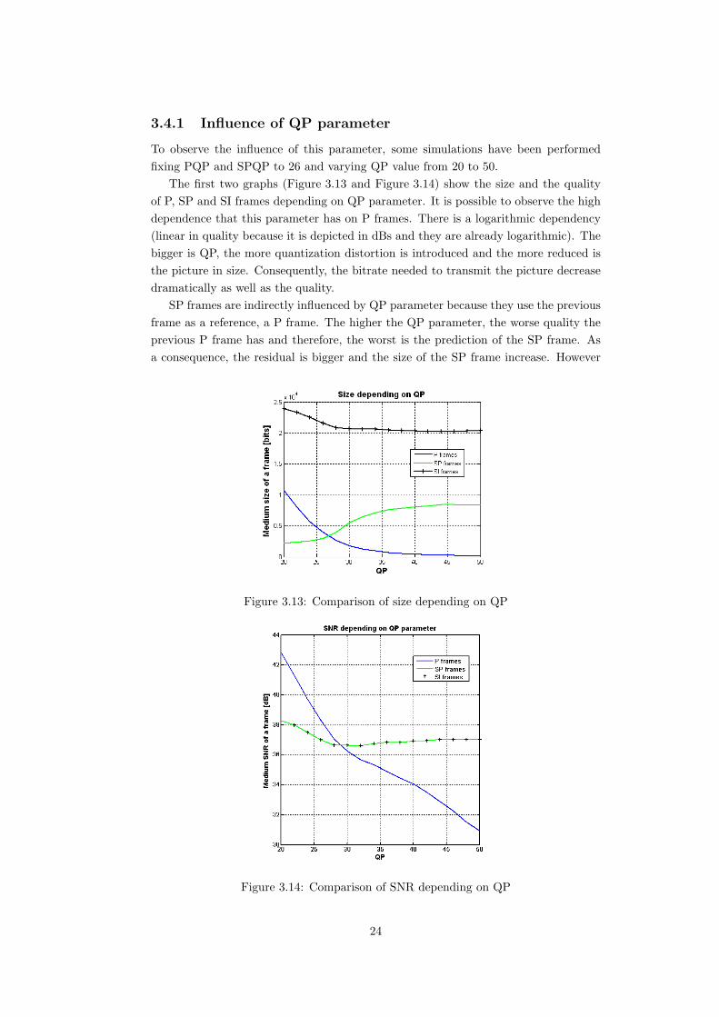
3.4.1 Influence of QP parameter

To observe the influence of this parameter, some simulations have been performedfixing PQP and SPQP to 26 and varying QP value from 20 to 50.

The first two graphs (Figure 3.13 and Figure 3.14) show the size and the qualityof P, SP and SI frames depending on QP parameter. It is possible to observe the highdependence that this parameter has on P frames. There is a logarithmic dependency(linear in quality because it is depicted in dBs and they are already logarithmic). Thebigger is QP, the more quantization distortion is introduced and the more reduced isthe picture in size. Consequently, the bitrate needed to transmit the picture decreasedramatically as well as the quality.

SP frames are indirectly influenced by QP parameter because they use the previousframe as a reference, a P frame. The higher the QP parameter, the worse quality theprevious P frame has and therefore, the worst is the prediction of the SP frame. Asa consequence, the residual is bigger and the size of the SP frame increase. However

Figure 3.13: Comparison of size depending on QP

Figure 3.14: Comparison of SNR depending on QP

24

this parameter has no influence on the quality of the SP frame because it is not aquantization parameter of these frames, and thus they do not introduce quantizationdistortion. SI frames, since they do not use previous P frames as a reference forprediction, are not affected by QP parameter.

P frames use inter prediction, and therefore they utilize the previous frames asa reference. In our video application, only the previous frame is utilized because thebuffer size is set to one. The behaviour of P frames has also been studied depending onwhether they are just after an SP or an SI frame, and the rest of P frames (Figure 3.15and Figure 3.16). In general terms, SP and SI frames are worse in quality than P and

Figure 3.15: Comparison of size of P frames depending on QP

Figure 3.16: Comparison of SNR of P frames depending on QP

25

I frames. That is the reason of the bigger size of P frames just after SP frames forlow QP parameters. Their reference is worse and therefore their prediction so moreresidiual is transmitted. However, the higher the QP, the more the quality of P framesdecrease whereas the SP and SI quality is maintained stable. In these circumstances,SP frames are a better reference than P frames and the behaviour of the P framesafter the SP or SI frames improve, outperforming the other P frames.

3.4.2 Influence of PQP parameter

Simulations have been performed fixing QP and SPQP parameters to 26 and varyingPQP from 20 to 50. The two figures depicted next (Figure 3.17 and Figure 3.18) showthe influence that this parameter has in the size and in the quality of SP, SI and Pframes. The effect of this parameter is clear in SP frames. The residual obtained tobe transmitted is quantized by this parameter and therefore the size of SP frames de-crease logarithmically with PQP. The higher the PQP means also a bigger quantizationdistortion and a worse quality for the reconstructed image.

The reconstructed image is the same for SP and SI and thus SI quality also decreaseswith the increase of PQP. On the contrary, this parameter has no relevant influenceon the size of SI frames.

The behaviour of P frames regarding this parameter is better shown in Figure 3.19where P frames are divided between the frame just after an SP or an SI frame, andthe rest. As it has been mentioned before, P frames uses only the last frame as areference. P frames just after an SP or an SI frame use those as a reference whosequality decrease for high PQP. In those cases, the prediction is worse and consequentlymore bits are sent. However the other P frames use other P frames, with good qualityeven for high PQP, as a reference, resulting a proper prediction and a small residual.The size of these frames do not increase with high PQP.

On the other hand, this parameter has no influence on the quality of these twoframes because they are not quantized by this value and therefore no quantizationdistortion is introduced.

Figure 3.17: Comparison of size depending on PQP

26

Figure 3.18: Comparison of SNR depending on PQP

Figure 3.19: Comparison of size of P frames depending on PQP

3.4.3 Influence of SPQP parameter

Simulations has been performed fixing QP and PQP parameters to 26 and varyingSPQP from 20 to 50.

The two figures depicted next (Figure 3.20 and Figure 3.21) show the influence ofthis value on the size and the quality of P, SP and SI frames. In SI frames, the residualis quantized by this parameter and thus the size of the transmitted data is reducedby increasing SPQP. Moreover, there will be more quantization distortion affectingthe quality of the reconstructed picture. SPQP does not quantize the residual ofSP frames, and that is the reason why their size do not depend on this parameter.However, in order to have identical reconstructed images in both, SP and SI frames,the decoded image is quantized and dequantized by SPQP. consequently, SP qualitydecrease when this parameter becomes higher.

The behaviour of P frames is better explained in Figure 3.22 where there is a

27

Figure 3.20: Comparison of size depending on SPQP (PQP=26)

Figure 3.21: Comparison of size depending on SPQP (PQP=26)

Figure 3.22: Comparison of size of P frames depending on SPQP (PQP=26)

28

distinction between P frames just after an SP or an SI frame and the rest of P frames.As in previous cases, P frames use only the previous picture as a reference. If quality ofSP or SI frame decrease, the prediction of the P frame just after those, becomes worse.Consequently, the residual size increases and therefore the amount of transmitted data.However, its quality is maintained stable, since this parameter is not a quantizationparameter for these frames. The other P frames that use other P frames with goodquality as a reference do not depend on SPQP, neither in size nor in quality.

All these conclusions are true until a certain SPQP value. SI macroblocks can onlybe codified as I macroblocks whereas SP can be codified as P or I macroblocks. Thedecision of the type of prediction is made in the encoder in the function that encodesone macroblock [16], and the simplified algorithm is explained in Figure 3.23.

Figure 3.23: Algorithm to decide the encoding mode of a MB

29

The information about the type of macroblock has been extracted from the tracefile of the encoder (Figure 3.24). The trace file explains deeply the different fieldsof the encoded bitstream. At the beginning of the information that describes everymacroblock there is a section called mb type with a number. If this number is smallerthan five it is a P macroblock and if it is five or more it is a I macroblock. mb type

Figure 3.24: Extract of the trace file.

Figure 3.25: P macroblocks types.

30

equal to five corresponds to I4x4 macroblocks and greater to 5 corresponds to I16x16.The types of macroblocks are described in Figure 3.25 and Figure 3.26 [16]. I

macroblocks come after P macroblocks and therefore 4 must be added to the mb typenumber in Figure 3.26.

When SPQP increases, the distortion of P macroblocks in SP becomes so high thatthe encoder finds better to encode using intra prediction in blocks known as I16x16.Consequently, the size increase as well as the quality of the reconstructed image.

I macroblocks in SI frames also change from I4x4 to I16x16. This bigger blocksare more difficult to be predicted using spatial prediction since spatial correlation

Figure 3.26: I macroblocks types.

31

decreases between big portions of a picture. The residual becomes bigger and morebits are transmitted. The quality of the reconstructed image improve because the sameis used for both, SP and SI frames. For high SPQP values, both SP and SI frames areformed by I16x16 blocks, and thus they become very similar. That is the reason whySP and SI size converge in these cases.

The effect of the improvement in the quality of the reconstructed image of an SPor an SI frame affects clearly the first P frame just after them. A better reconstructedimage means a better reference, a better prediction and a smaller residual. Therefore,less bits are transmitted.

In the graphs shown below (Figure 3.27 and Figure 3.28), it is possible to observethat the SPQP value where the two types of macroblocks cross, coincide with the SPQPvalue where a peak in size and quality was observed, the point where the behaviourchange.

The value of the SPQP parameter from which P macroblocks in SP frames become Imacroblocks depends on the value of PQP. In previous simulations PQP parameter was

Figure 3.27: Type of macroblocks in an SP frame

Figure 3.28: Type of macroblocks in an SI frame

32

Figure 3.29: Comparison of SNR depending on SPQP (PQP=28)

fixed to 26 and in the figure depicted below a PQP of 28 has been used (Figure 3.29).QP value is fixed to 26 and SPQP parameter varies from 20 to 50. The peak in sizehas displaced from SPQP 34 to 36. At this point there are more I macroblocks thanP macroblock, improving the behaviour in quality and increasing the bitrate.

A higher PQP value means more quantization distortion for the reconstructedimage in SP and SI, and that means a worse quality. In those cases, the effect of thedistortion introduced by SPQP is in some way concealed until a higher value of thisparameter.

QP parameter does not displace the SPQP value where P macroblocks becomes Imacroblocks, that produces this peak in quality.

3.5 Description of the optimized values for SPQP

and PQP

In the previous section, the effect in rate and distortion of the different quantizationparameters have been described. General conclusions are that PQP influence size ofSP and quality of SP and SI frames whereas SPQP afects size of SI and quality of SPand SI frames. Figure 7.3 [17] depicts how the increase of SPQP parameter decreasethe size of SI frames and increase the distortion of SP frames.

These conclusions explains the behaviour, however optimized values were seek forthis project. The choice of the values of these parameters have followed the recom-mendation described in [18].

In the considered scenario, SP frame positions are spaced regularly in the trans-mitted video stream and SI frames can be sent in these positions in case of packetlosses to stop error propagation. The proportion of SI frames transmitted instead ofSP frames depends on the packet error rate and on the SP period. The probability oftransmitting an SI frame at an SP frame position is denoted as x. In this optimiza-tion, the quality is considered as a constraint and the bit-rate is minimized what isequivalent to minimizing the expected size of a frame sent at an SP position:

33

Figure 3.30: Distortion of SP frames and size of SI frames depending on SPQP

Min. R = xRSI + (1− x)RSP1 (3.1)

s.t. DSP1 = DSI = D (3.2)

where RSI , RSP1 , DSI and DSP1 denotes the rate and distortion of SI and primarySP frames respectively.

The optimization is carried out by minimizing the bitrate of the transmission fora given distortion, that means that a minimum value of quality must be exceeded.This optimization method is described with more detail in Appendix A, and all themathematical explanations are written in [18].

This method concludes that the only possible optimum values are those shown inTable 7.1 , as well as the optimal values derived empirically. Empirical values havebeen used in these project.

x model ≤ 0.2 ≥ 0.2 and ≤ 0.5 ≥ 0.5x empirical ≤ 0.1 ≥ 0.1 and ≤ 0.2 ≥ 0.2PQP QP - 1 QP - 2 QP - 3SPQP QP - 10 QP - 5 QP

Table 3.1: Optimal values for PQP and SPQP

34

Chapter 4

Modifications in the encoder

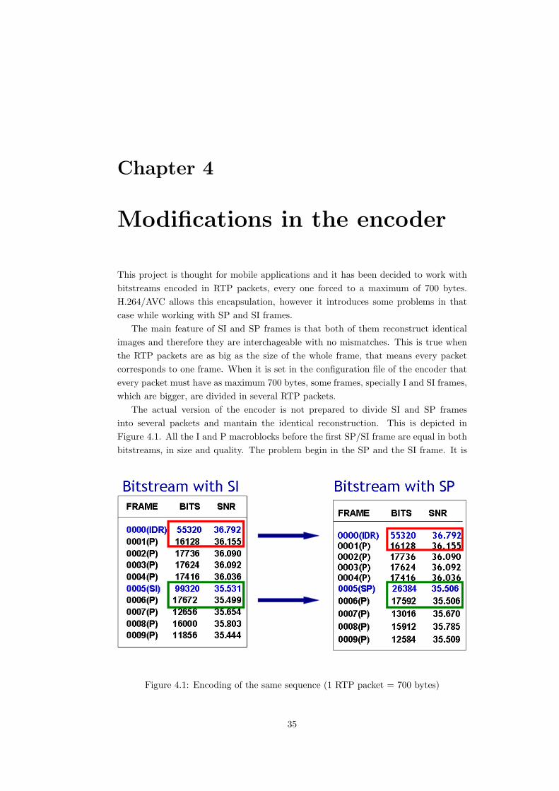
This project is thought for mobile applications and it has been decided to work withbitstreams encoded in RTP packets, every one forced to a maximum of 700 bytes.H.264/AVC allows this encapsulation, however it introduces some problems in thatcase while working with SP and SI frames.

The main feature of SI and SP frames is that both of them reconstruct identicalimages and therefore they are interchageable with no mismatches. This is true whenthe RTP packets are as big as the size of the whole frame, that means every packetcorresponds to one frame. When it is set in the configuration file of the encoder thatevery packet must have as maximum 700 bytes, some frames, specially I and SI frames,which are bigger, are divided in several RTP packets.

The actual version of the encoder is not prepared to divide SI and SP framesinto several packets and mantain the identical reconstruction. This is depicted inFigure 4.1. All the I and P macroblocks before the first SP/SI frame are equal in bothbitstreams, in size and quality. The problem begin in the SP and the SI frame. It is

Figure 4.1: Encoding of the same sequence (1 RTP packet = 700 bytes)

35

normal that every of them have a different size because spatial prediction used in SIframes is not so accurate as inter prediction and therefore the number of residual sent isbigger. However the quality of the reconstructed image is also different. Consequently,the next P frames use different references for the prediction and that is the reason whythey do not coincide in size and quality.

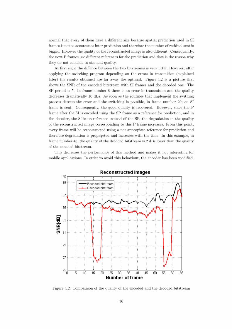
At first sight the diffence between the two bitstreams is very little. However, afterapplying the switching program depending on the errors in transmision (explainedlater) the results obtained are far away the optimal. Figure 4.2 is a picture thatshows the SNR of the encoded bitstream with SI frames and the decoded one. TheSP period is 5. In frame number 8 there is an error in transmision and the qualitydecreases dramatically 10 dBs. As soon as the routines that implement the swithingprocess detects the error and the switching is possible, in frame number 20, an SIframe is sent. Consequently, the good quality is recovered. However, since the Pframe after the SI is encoded using the SP frame as a reference for prediction, and inthe decoder, the SI is its reference instead of the SP, the degradation in the qualityof the reconstructed image corresponding to this P frame increases. From this point,every frame will be reconstructed using a not appropiate reference for prediction andtherefore degradation is propageted and increases with the time. In this example, inframe number 45, the quality of the decoded bitstream is 2 dBs lower than the qualityof the encoded bitstream.

This decreases the performance of this method and makes it not interesting formobile applications. In order to avoid this behaviour, the encoder has been modified.

Figure 4.2: Comparison of the quality of the encoded and the decoded bitstream

36

The idea is to send I and P macroblocks divided into blocks of 700 bytes, but to sendSP and SI frames as an only packet. This has been considered a proper solution toobtain realistic results of the behaviour of the method because of how the errors aresimulated in the switching program, but this is explained in the next chapter.

A simplified algorithm of the encoder is depicted in Figure 4.3. The changes per-formed on it are remarked with an orange square. The slice mode is previously arrengedin the configuration file, where it is set:

SliceMode = 2 # Slice mode (0=off 1=fixed #mb in slice 2=fixed# # bytes in slice 3=use callback)

SliceArgument = 700 # Slice argument (Arguments to modes 1 and 2 above)

Figure 4.3: Modification of the encoder

37

So the slice mode is set to 2, what means that the RTP packets have a fixed numberof bytes and equal to 700. The changes are located in the function that encodes onemacroblock, before its parameters are initialized, since this initialization depends onthe slice mode. If the macroblock belongs to an SI/SP the slice mode changes toNO SLICE, what means that the whole frame is encapsulated in an only RTP packet.

With this method SI and SP reconstruct exactly the same image, and consequentlythe next P frames use the same picture as a reference and are identical in the twobitstreams. In Figure 4.4 it is shown the bitstream encoded with SI inserted and thebitstream decoded with errors. The errors are in the same positions as in Figure 4.2,however, after the SI, the decoded bitstream recovers the good quality not only in thisframe, but also in the next P frames, just until there is another error in frame number52.

All simulations discribed in chapter 3 have been performed with the encoder alreadymodified.

Figure 4.4: Quality of the encoded and the decoded bitstream after the modification

38

Chapter 5

Implementation of the

switching process

5.1 General scheme

The aim of the project is to implement a switching process between the two new framesthat H.264/AVC standard includes regarding to prior standards, SP and SI frames.Depending on the error information received from the decoder, it is decided to send anSI frame, formed using spatial prediction. The no abscence of previous frames helpsto stop the error propagation while decoding.

The H.264/AVC encoder is able to produce a sequence with some SP or SI frameswithin the bitstream in periodical locations. However, the encoder does not decidewhether to encode an SP or an SI depending on the error information recieved, thatmeans that the switching process is not implemented inside the encoder. A generalscheme is shown in Figure 5.1, where the switching program is depicted between theencoder and the decoder.

The switching process is implemented in a Matlab routine with some inputs andan output (Figure 5.2). The encoder codifies the sequence twice, one with SP framesand the other with SI frames inside. Both bitstreams must have the same periodicityfor the switching frames and the same encoding properties, for instance the quantiza-tion parameters (QP, PQP and SPQP). An example of the bitstream with SP framesinserted with an SP periodicity of 4 is shown in Figure 5.3. The two bitstreams beginwith an I frame. All frames from one bitstream reconstruct identical images to thecorresponding frames in the other bitstream. Also the size is the same for I and Pframes to the corresponding frames from the other bitstream. These bitstreams are

Figure 5.1: Diagram of the location of the switching process

39

Figure 5.2: Bitstreams with SP and SI frames inserted.

Figure 5.3: Inputs and outputs of the switching routine.

two of the inputs of the Matlab routine.The third input is the error information that points out when the switching must be

implemented. The output is one bitstream with SP and SI frames inserted periodically,depending on the error information. This output is transmitted and is what thedecoder recieves in case of no error in transmision.

5.1.1 UMTS. General transmision scheme

This project is based on video applications transmitted over UMTS networks. Uni-versal Mobile Telecomunications system (UMTS) is a technology used for mobiles ofthird generation, succeed of GSM. It is nowadays being developed into a fourth gene-

40

Figure 5.4: Simplified scheme of the UMTS network

ration technology. UMTS normally works over a WCDMA interface and over GSMinfraestructures.

UMTS is not limited to mobile applications. Its three main features are its multi-media capabilities, a high internet access speed and the possibility of real time video.The voice quality is comparable to that of the fixed line telephone and it providesa wide variety of services like videoconferencing and live TV. Figure 5.4 depicts asimplified scheme of a UMTS network.

The UMTS network structure consits of two big subnetworks, a telecomunicationnetwork and a management network. The first one deals with the support of the trans-mition of information between the extrems of a conection. The second one controlsthe registration, definition and security of the service profiles provided as well as it hasthe misison of detecting and solving posible breackdowns and anomalies in the net.

The telecomunication network have the following two elements:

• Core Network: It includes transport and inteligence functions. The transportof the information and the signaling data and its conmutation is supported bytransport functions whereas routing is considered as an intenligence function.Throughout the core network, UMTS is conected to other networks to makepossible the communication not only with users from UMTS.

• UMTS Terrestrial Radio Access Network (UTRAN): Developed to ob-tain high velocities in transmition, conects mobile stations with the core network.It is formed by a series of Radio Network Subsystems (RNS), which are respon-

41

sible of the resources, the transmision and the reception in a set of cells.

The RNS is made up in turn of one Radio Network Controller (RNC) and one orseveral NodeB. Node Bs are also referred to as Base Transceiver Stations (BTS)or Base station in GSM. It has a radio frequency trasnmitter and reciever tocommunicate directly with the mobiles of its corresponding cell.

The RNC is responsible of controlling the UTRAN and therefore the NodeB ofone or more Base Transceiver Stations (BTS).BTS are controlled by the RNCand therefore it has not a lot of functionalities. Some of the tasks that the RNCpresent are:

– Admission control

– Packet scheduling

– Security functions

– Handover control

• User Equipment (UE): This is the new terminology in 3G of what is wasknown as Mobile Station in 2G. It is made up of a mobile terminal, that isthe end-point of the radio interface, and a USIM (Universal Subscriber IdentityModule). The USIM is roughly the SIM of GSM, and it stores information of theuser for its identification in the network as well as other informations as mobilenumber, contacts and short messages.

In UMTS networks, the videos are stored in the Media Server. The Media Server isdefined as a device that stores and shares media. The different types of media (video,photos, audio) are stored on its hard drive. With an special application it is possible tomake this information accesible to users from a remote location via internet. Becauseof its vague definition, a media server only requieres a method of storing media anda network connection. Thus several devices can be considered Media Server, as amedia center PC, or a commercial web server that hosts media. Depending on theapplication, a powerful processor, big RAMs for large storage or high access speedmay be needed. Some Media Servers are able to capture the media using specializedhardware as TV turner cards. In case of analog video, it has to be encoded in digitalformat before being stored on it.

Video applications are transmitted over UDP. UDP is a transport level protocol,very useful for real time applications because it does not waste resources in controllingthe parameters of the link, like flow control. Consequently the different packets canbe received out of order. A previous conection before trasnmitting is not necessarybecause a UDP datagram incorporates enough address information on its header toallow the end-to-end communication. Since it does not make error control, there isno information of whether a packet has been recieved correctly or not, and thereforeno retransmission is possible. This is the main difference with the other very impor-tant transport protocol, TCP, which is reliable. However, for real time applications,retransmissions are not allowed because of the little delays required.

42

5.1.2 Location of the Switching program in the UMTS network

Depending on several features of the network, different locations within the UMTSnetwork are more interesting for the switching program. In this project two are ex-plained:

• Media Server:

This is the device where the videos are stored. The main advantage of thislocation is that both bitstreams, one with SP and the other with SI framesinserted, must not be transmitted, only the result of the switching process, savingbandwidth in the transmission. To make the switching possible, informationabout how the packets have been recieved is needed. As it has been explainedbefore, UDP does not inform about errors in transmission and therefore a higherlevel is used to know whether the switching must be implemented or not.

RTP is the higher protocol over which the UDP datagrams are transmitted(Figure 5.5). RTP is utilized together with RTCP to provide information aboutthe quality of data distribution. The video is sent from the Media server tothe client in RTP packets, transparent to other devices of the network becauseit is an end-to-end protocol. RTCP is used to monitor the quality of service,providing out-of-band control information. RTCP packets do not transmit data,but contains stadistics that reports over the number of packets sent, the num-ber of packets lost, the interarrivel jitter, etc. RTCP packets are sent over an

Figure 5.5: Switching program located in the Media Server

43

independent feedback channel.

The main drawback of this location is the delay on the reporting messages intro-duced by the feedback channel. This delay prevents the sender from adaptingto the real state of the session. In our application, the switching could be im-plemented a long time after the error has started propagating, causing a greatdegradation of the quality in the decoded video.

• Radio Network Controller:

The RNC is the device that controls the UTRAN. To make possible the im-plementation of the switching in the RNC, both bitstreams, the one with SIframes inserted and the other with SP, must be transmitted until this point ofthe UMTS Network (Figure 5.6). This suppose an increase in the bandwidthneeded to transmit the video information, not only because the P frames haveto be transmitted twice, but because the SI frames are much bigger than P andSP frames.

The main advantage is that the RNC is closer to the Mobile Station than theMedia Server and therefore the time needed to transmit some information fromthe Mobile Station is smaller. The RNC does not understand the transportprotocol (RTP/RTCP), and therefore the error information must be transmittedin the link layer or a lower one.

Figure 5.6: Switching program located in the Radio Link Controller

44

5.2 Program performance

5.2.1 Overview

The program performed implements the switching process and also simulates differentsfeatures of the UMTS network. The challenge of implementing the system in a realUMTS network could be an interesting continuation of this project. In a real situa-tion, specially for real time applications, as soon as the RTP packets are encoded theprogram should recieve them and decide wether to switch or not. In this simulationthe whole encoded sequence is avalaible in the program.

The output of the Switching Program is directly decoded, and therefore no trans-mission channel have been used. No errors would be in the decoded bitstream and noswitching would be implemented. As a conscequence, the errors in transmission havealso been simulated in the program following the information from the error file.

The error information should be received a little time after the error in transmissionhas occured, applying the switching in case of error as soon as there is an SP frame.However, the delay of the feedback channel and the error information have to besimulated also from the error file.

Figure 5.7 shows the different routines of the Switching Program as well as itsinputs and outputs. Both bitstreams, one with SP and the other with SI framesinserted, are inputs of save vectors, a routine that divides its RTP packets into severalfields, extracting some information about them. This data is used later to help in theimplementation of the switching. These fields and information are stored in vectorssaved in memory.

Simulate Different Delays routine has the error file and the delay as inputs. Theuser decides which delay the feedback channel has, depending on the desired UMTSnetwork enviroment to be simulated. This routine also loads the vectors with theinformation about the RTP packets.

With the information about the errors, the RTP packets and the delay, the switch-ing is implemented in Main Switching routine. This function calls other functions thatsimulates the errors in transmission extracting the information from the error file, andalso the delay of the feedback channel.

Since a comparison with the performance of bitstreams with only I and P framesis a part of this project, also the errors in transmission must be simulated for thesebitstreams. However, no switching is implemented since I frames are always sent withthe same periodicity and therefore the information about the delay in the feedbackchannel is useless. Consequently, routines used for bitstreams with SI frames aredifferent to those utilized for bitstreams with SP frames inserted.

The bitstream with errors inserted and the switching implemented to be decoded isone of the outputs of the program but not the only. Some text files have been createdduring the implementation to inform about different aspects which will be useful next.These files includes information about the size of the bitstreams, the probability ofsending an SI frame instead of an SP frame and also information about the RTPpackets.

45

Figure 5.7: Routines of the Switching Program

46

5.2.2 Extraction of the RTP packets

The first part of the switching program consits of various routines that extract thedifferent fields of the RTP packets resulted from the encoder (Figure 5.8). In a realcase, not the whole bitstream would be avalaible to be extracted (obvious in real timeapplications).

The different parts of the bitstream are saved into two vectors, and every elementcorrespond to one packet. In one of these vectors the information is saved in the sameformat as it is in the encoded bitstream in order to directly be used in the switching.Both bitstreams with SP and with SI frames inserted must be saved to implementlater the switching. The other vector, stores some interesting information decodifiedfrom the RTP packet that will be needed to implement the switching.

Figure 5.8: Routines to extract RTP packets

The main routine consist of a loop that runs all the packets of the bitstream. Theinformation is extracted from the packet. But the bitstream is a string of bits with noapparent division between each packet. However the encoder has added some bytes atthe begining of every packet informing about its length. The process is described inFigure 5.9 and explained next.

The first four bytes corresponds to the length of the RTP packet including itsheader. This information is codified in little endian. In the example depicted, thelength is equal to 21. Afterwards there are 4 syncronization bytes which bits arealways equal to 1. The packet header is always equal to 13 bytes, 12 corresponding tothe RTP header and one to the NALU header (NALU is the term used to talk aboutNAL units, packets in which the coded video is organized). With this information itis very easy to calculate the length of the payload, just by substracting headers lengthto the length of the whole packet. In the example of the picture 21 - 13 = 8 is thelength of the payload. Consequently the next 13 bytes corresponds to the header andthe following 8 bytes to the payload of the packet.

47

Figure 5.9: RTP packets output from the encoder

Figure 5.10: First bits of the RTP payload extracted from the trace file.

Besides, some useful information is extracted from the payload, the slice type andthe frame number corresponding to this packet. This information will be used in theswitching to help on its impelementation. Here above there is an example of the firstbits from the payload, extracted from the trace file (Figure 5.10) :

The pic parameter set id is always 1 bit and the frame num corresponds to a fixednumber of bits (four in this example). However first mb in slice and slice type arecodified in such a way that the number of zeros that precede the bits of informationare always one bit less that those. In this example, the first mb in slice is equal to0000001100011, and there are 6 zeros (000000) before the first 1, that means that theinformation bits (1100011) are 6 + 1 = 7 bits.

At the end, the two vectors with the information about the RTP packets are storedin memory in order to be used later in the switching. The reason of this storage is toavoid this operation when it is wanted to simulate the same bitstream but with severaldelays (no extraction is needed but only to load this vectores from memory).

48

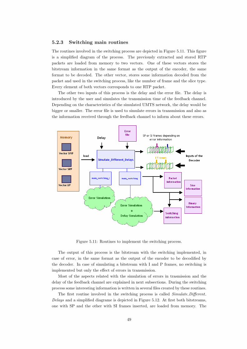
5.2.3 Switching main routines

The routines involved in the switching process are depicted in Figure 5.11. This figureis a simplified diagram of the process. The previously extracted and stored RTPpackets are loaded from memory to two vectors. One of these vectors stores thebitstream information in the same format as the output of the encoder, the sameformat to be decoded. The other vector, stores some information decoded from thepacket and used in the switching process, like the number of frame and the slice type.Every element of both vectors corresponds to one RTP packet.

The other two inputs of this process is the delay and the error file. The delay isintroduced by the user and simulates the transmission time of the feedback channel.Depending on the characteristics of the simulated UMTS network, the delay would bebigger or smaller. The error file is used to simulate errors in transmission and also asthe information received through the feedback channel to inform about these errors.

Figure 5.11: Routines to implement the switching process.

The output of this process is the bitstream with the switching implemented, incase of error, in the same format as the output of the encoder to be decodified bythe decoder. In case of simulating a bitstream with I and P frames, no switching isimplemented but only the effect of errors in transmission.

Most of the aspects related with the simulation of errors in trasmission and thedelay of the feedback channel are explained in next subsections. During the switchingprocess some interesting information is written in several files created by these routines.

The first routine involved in the switching process is called Simulate DifferentDelays and a simplified diagrame is depicted in Figure 5.12. At first both bitstreams,one with SP and the other with SI frames inserted, are loaded from memory. The

49

Figure 5.12: Simplified algorithm of Simulate Different Delays routine.

different delays introduced by the user are simulated one after the other. For everydelay the error file is utilized from its beginning in order to simulate with the sameerror environment for all of them. The error file have much more information that theneeded for the transmission of only one bitstream. To make it more realistic, the samebitstream is simulated several times, using different parts of the error file, to show theeffect of errors in differet points of the bitstream.

In case of simulating a bitstream with only I and P frames inserted, the delay is notneeded because no switching is implemented (only the effect of errors in transmissionaffects the bitstream).

The routine that includes the main loop of the switching process is called MainSwitching and its simplified algorithm is shown in Figure 5.13. Its inputs are thevectors with SP and the SI bitstreams, the error file and the delay introduced by theuser. The main loop runs all the packets of the bitstream.

First, the type of frame of the current packet is controlled. Only in case it corres-ponds to an SP frame the switching condition is checked. If it is set to one, it is apacket from an SI frame, that means that the switching is going to be implemented.The way to perform it, is assigning all the packets corresponding to the SI frame withthe same frame number from the SI bitstream to the vector that stores the packets ofthe final bitstream. If this condition is equal to zero or the packets corresponds to an Ior a P frame, the switching is not implemented and the packet from the SP bitstreamis assigned to the vector with the final bitstream.

The switching condition is obtained from the routine called Calculate Conditionsand explained later. The packets are assinged to the final bitstream only in case the

50

Figure 5.13: Simplified algorithm of Main Switching routine.

lost packet condition is set to zero but this is part of the error simulation and is alsodescribed later.

The main routine of the process for a bitstream with only I and P frames inserted iscalled Main Switching I and its simplified algorithm is shown in Figure 5.14. The prin-cipal difference with Main Switching routine is that since no switching is implemented,

51

Figure 5.14: Simplified algorithm of Main Switching I routine.

it is not needed to control the type of frame and there is no switching condition. Onlythe effect of the errors is simulated by assigning or not the packets from the orignalbitstream to the vector that stores the final bitstream.

The different files created during the execution of these routines try to informabout several aspects of this process. In the so-called Packet information file, thedifferent bitstreams are divided into packets, informing about the frame they belongto, the number of bits of the header and the payload and the number of packet. TheSize information file contains the total number of bits and the bitrate of the finalbitstream, previously calculated in the Main Switching routine. There is another filewith the information about the bitstreams in bynary data. The last one, the Switchinginformation file describes deeply the switching process, informing about when thetransmission is affected by an error and when the error is detected by the system.

The final bitstream resulted after this process is stored also in a file with properformat to be decoded by the decoder.

5.2.4 Error simulation

Avoid propagation of the errors occured during data transmission is the aim of SP andSI frames. In order to obtain good results these errors must be simulated in a realisticform.

Most of the errors occur in the wireless link between Node B and the Mobile Station.The error file uses information about the errors detected in this link, measured usinga mecanism shown in Figure 5.15. In the UMTS Terrestrial Radio Access Network(UTRAN), where the errors have been detected, the IP packets are segmented intoTransport Blocks (TB) [19]. Every Transport Block has a CRC field attached, whichsize can be configurable to 0,8,12,16 or 24 bits. This field is checked in the Mobile

52

Figure 5.15: Error file: origin and format.

Station to detect errors in transmission. In case of no error in a TB, a 0 is written in theerror file and if an error is found, a 1 is set. Normaly errors occur in bursts, describedby several 1s together in the error file. This would be the information transmittedthrough the feedback channel.

Routines involved in error simulation are depicted in Figure 5.16. It can be ob-served that this process affects both, bitstreams with SP frames inserted and bitstreamswith only I and P frames.

The number of values to read from the error file are calculated in number TB andthis routine is called by Main Switching. To be realistic in the simulation, only the

Figure 5.16: Routines involved in the error simulation.

53

Figure 5.17: Fragmentation of an RTP packet into Transport Blocks.

Figure 5.18: Discard process.

TBs of the packet we are working with at that moment, are read. However, the packetsof our bitstreams are RTP packets before being segmented by the UTRAN into TBs.In order to know in how many TBs every RTP packet would be divided, fragmentationis performed (Figure 5.17).

It is an IP packet what is fragented into TBs and therefore, the UDP and IPheaders must be added [19]. The UDP header are 8 bytes and the IP header are 20.For a data rate below 384kbits/s, the payload of a Radio Link Controller (RLC) is320 bits and 640 bits for higher data rates. A TB corresponds to a RLC payloadand a header, which size depends on whether they work in acknowledged mode (AM),allowing RLC packet retransmission or in unacknowledged mode (UM) where the erroris only detected and no feedback is allowed.

However the size of this header is not important to calculate the number of TBs,since it is the same as the number of RLC payloads. In our simulation we workwith data rate below 384kbits/s and consecuently the number of TBs is resulted fromdividing the number of bits of the IP packet to 320:

Number TBs =RTP Packet+ UDP Header + IP Header [bits]

320(5.1)

54

As it has been mentioned before, this number of TBs informs us about the numberof values to check in the error file. The reading of these values is performed in de-cide packet lost routine. If among these values there is one or more 1s, then an errormust be simulated, setting the switching condition to 1. This condition is utilize inMain Switching to simulate the error by copying the packet from the original bitstreamto the final vector only if this value is equal to zero. In case of no errors, the outputis the original bitstream with SP frames inserted (Figure 5.18).

5.2.5 Delay simulation

The decoder detects that there is an error because the timing of decoding the framesbecomes not normal. So the decoder knows at the moment of decoding, that there hasbeen an error, but not the Radio Network Controller or the Media server, where theswitching is located. This information about the errors occured is sent back through afeedback channel which have a certain delay. This delay must be taking into accountin order to be realistic in the simulation.

The delay is introduced in the program by calculating the following equation:

delay[number of frames] = fps x delay[seconds] (5.2)

where fps is the number of frames per second of the video, what is a configurablefeature of the encoder. For an introduced delay value of the feeback channel it ispossible to calculate the number of frames that the system needs, to know about theerror.

Figure 5.19 depicts how the program works. In case of no errors, SP and P framesare sent. If an error is read from the error file, a packet is extracted from the bitstreamin order to simulate the error. From this point, and after the number of frames of delaycalculated by the equation, the system detects the loss of the packet, simulating thedelay of the feedback channel. But the SI frame is sent only instead of an SP frame,not replacing a P frame, and the error follows propagating until the switching point.After the SI frame, good quality is recovered.

Figure 5.19: Effect of the feedback channel delay.

55

As it has been mentioned before in Main Switching routine, if lost packet conditionis set to one, the current packet will not be copied to the final bitstream in order tosimulate the packet loss, and at this point, the frame where the system will detect theerror is calculated by:

error frame no = actual frame+ delay[number of frames] (5.3)

The variable switching condition is controlled by decide switching routine, whosesimplified algorithm is shown in Figure 5.20. Its value is only set to one in caseerror frame no = actual frame, what means that in a real case the data informingabout the packet loss would have been recieved.

The variable error frame no is only different to 0 when an error have been simulatedand the problem is not solved yet. When an SI frame is sent to solve the problem,both, error frame no and switching condition are initialized.

The effect of simulating the errors in transmission and the delay of the feedbackchannel is depicted in Figure 5.21. In this example there are two errors, one in framenumber 16 and the other in frame number 60. The difference in quality regarding tothe original bitstream is 15 dBs. The delay simulated is big, 1.5 seconds. As fps =10, the systems needs 15 frames to know about the packet loss. The good quality isrecovered as soon as there is a switching point, when an SI is sent. In these case, theSP period used is 5, and the system knows about the first error in frame number 31,therefore the problem is solved in frame number 35, the next multiple of 5. The seconderror is noticed in frame number 75 and the SI is sent in frame number 80.

The feedback delay is only simulated for bitstreams with SP frames inserted andnot for those with only I and P frames because they do not implement the switching,only the packet loss to compare their quality for a similar error environment.

Figure 5.20: Simplified algorithm of decide switching routine.

56

Figure 5.21: Graph showing the effect of a big delay.

57

Chapter 6

Simulation results

6.1 Simulation overview

The main objective of this project is to obtain a conclusion about the utility of thenew frame types introduced by the new video coding standard H.264/AVC, calledSP and SI frames. These new frame types have been designed with the intention ofrecovering the good quality while decoding after an error in transmission. This wasalready possible in previous standards with the existing frame types. By sending anI frame that uses no prior frames as a reference, it is possible to stop the error thatpropagated due to the usage of temporal dependencies. However, the size of a framethat uses spatial dependencies is much bigger than those with temporal dependencies.In previous methods, frames with spatial dependencies were sent periodically withouttaking into consideration if there had been an error or not. That can be considered asa waste of resources.

In the method that has been previously explained, the frames with spatial predic-tion, and therefore they are able to stop error propagation, are only sent in case of anotification of an error in transmission. The main advantage of these two frames istheir capability to adapt themselves to the channel situation. In this chapter a deepcomparison with the method of using I and P frames has been done in order to obtain

(a) Mother and Daughter (b) Foreman

Figure 6.1: Images of the two videos used.

58

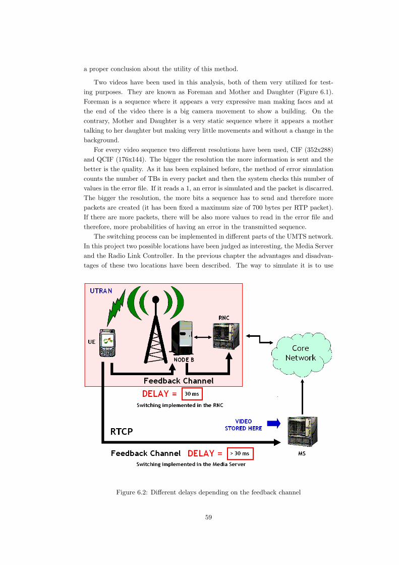
a proper conclusion about the utility of this method.

Two videos have been used in this analysis, both of them very utilized for test-ing purposes. They are known as Foreman and Mother and Daughter (Figure 6.1).Foreman is a sequence where it appears a very expressive man making faces and atthe end of the video there is a big camera movement to show a building. On thecontrary, Mother and Daughter is a very static sequence where it appears a mothertalking to her daughter but making very little movements and without a change in thebackground.

For every video sequence two different resolutions have been used, CIF (352x288)and QCIF (176x144). The bigger the resolution the more information is sent and thebetter is the quality. As it has been explained before, the method of error simulationcounts the number of TBs in every packet and then the system checks this number ofvalues in the error file. If it reads a 1, an error is simulated and the packet is discarred.The bigger the resolution, the more bits a sequence has to send and therefore morepackets are created (it has been fixed a maximum size of 700 bytes per RTP packet).If there are more packets, there will be also more values to read in the error file andtherefore, more probabilities of having an error in the transmitted sequence.

The switching process can be implemented in different parts of the UMTS network.In this project two possible locations have been judged as interesting, the Media Serverand the Radio Link Controller. In the previous chapter the advantages and disadvan-tages of these two locations have been described. The way to simulate it is to use

Figure 6.2: Different delays depending on the feedback channel

59

different delays for the feedback channel as it is shown in Figure 6.2.Using some information about different studies from the network, it has been con-

sidered that in case of implementing the process in the RNC, the delay of the feedbackchannel is about 30 ms. The next frame just after the error has occurred, the systemalready knows about it because of the way of simulating the delay (frames per secondused in the decoding is equal to 10). Bigger delays are simulated to consider also thecase of implementing the switching process in the Media Server. In case of simulatinga bitstream with only I and P frames, the delay does not affect the transission becauseno switching is implemented.

The whole simulation process is depicted in Figure 6.3. Firstly the bitstreams areencoded. The version of the encoder used is the one previously modified in ordernot to have problems with the reconstructed images while using SP and SI frames.All the modification process has been explained deeply in chapter 4. The encoder isconfigured to packetize RTP packets with a fixed size of 700 bytes. All videos have300 frames, but only 100 are codified because of skipping 2 frames every 3 (normalin video applications). This increases the information to send because there are moredifference between two consecutive codified images.

The velocity of encoding is set to 10 frames per second and that means that thevideo lasts 10 seconds. It can be considered as normal that every 10 seconds in anyvideo there is a change of sequence. In case of the bitstreams with SP or SI and Pframes, there is an I frame at the begining of the sequence because there is no previouspicture to which temporal prediction can refer. The multipicture buffer is the placewhere previous pictures are stored to be used as a reference for this type of prediction.In our simulation its size is set to one, so only the last picture is used as a referencefor P and SP frames.

The extended version of H.264/AVC is used because it is the only profile where theusage of SP and SI frames is allowed. The value of the QP, quantization parameterof the P and I frames, is the main configuration parameter to control the bandwidthneeded. It has been selected to work for the two videos in CIF resolution for a bit-

Figure 6.3: Simulation process

60

rate of about 220 kbits per second and for the two vidos in QCIF resolutions for abitrate of about 80 kbits per second. Several values around these mentioned havebeen simulated to observe the behaviour in their surroundings. The PQP and SPQPvalues, quantization parameters of SP and SI frames, have been chosen following therecomendations explained in chapter 3.

Different GOP (for bitstreams with I and P frames) and SP periods (for bitstreamswith SP or SI and P frames) are encoded to observe its influence on the performanceof the system.

The encoded sequences are processed by the program that implements the switchingprocess, performed in Matlab. For every bitstream different delays of the feedbackchannel are simulated. With a bitstream and a delay value, different parts of the errorfile are read to have different error situations simulated and make the whole systemmore realistic.

All the simulated bitstreams are decoded and the obtained results are processedby some programs, averaging the resulting values from the different errors situationssimulated. Several graphs have been depicted and the most relevant are analysed innext sections.

The whole process last plenty of time not only because of the enormous numberof simulations performed but also because of the encoding and decoding time needed,that is quite long. Even though it is true that the complexity of the encoding anddecoding process is important, the system nowadays is rather inefficient from thispoint, specially for real time applications. The code of both, the encoder and decodershould be optimized, although it is also important to point out that this is normalwhen a standard is stil developing.

6.2 Encoding step

The first step of the simulation is the encoding of every video for different QP parame-ters in order to obtain results for different bitrates that will help to see more clearlytheir behaviour. In order to compare the two different methods, not only the twobitstreams with SP and SI frames inserted are encoded but also a bitstream with onlyI and P frames. For the three bitstreams similar values of bitrates have been seeked.

The first graph Figure 6.4 depicts the different efficiency for the two resolutionsused, CIF and QCIF in case of using a bitstream with SP frames inserted. In thisexample shown, the video utilized is Mother and Daugther. It is possible to observethat QCIF resolution offers a better behaviour, since for the same number of bits sent,the quality is more than three dBs higher.

Another important aspect to remark is shown in Figure 6.5. A bitstream with Iand P frames codified, from Mother and Daugther in QCIF resolution, is depicted.The intention of this graph is to analyse the effect of using different GOPs. The biggerthe GOP, the best behaviour it has, and the difference between using a GOP of 5 anda GOP of 50 frames is 2.5 dBs. The same behaviour has been observed in other videos.The reason is found in the bigger size of I frames (spatial prediction). The smaller theGOP, the more I frames there are and therefore the less efficient the transmission isin case of having no errors. Of corse the more prepared to stop error propagation is

61

Figure 6.4: Comparison of QCIF and CIF resolution efficiency

Figure 6.5: Different GOPs for Mother and Daughter QCIF

this bitstream.The case of using different SP periods for a video sequence is not shown since the

difference in the efficiency is very little and it has been cosidered as irrelevant. The onlypoint to remark is that if we compare the SP bitstream with a bitstream of the samevideo with I and P frames (the GOP and the SP period is the same), the efficiency ismuch better for the SP bitstream. That is because of using temporal prediction always.For the SI bitstream the difference for different SP periods is extreamly important. InMother and Daughter CIF it is of 6 dBs. For the same desired quality, more bitrate

62

Figure 6.6: Comparison of quality for bitstreams with SP/P, SI/P and I/P frames

is needed for a bitstream with I frames inserted than for an SP bitstream, but stillmore bitrate than for an SI bitstream (Figure 6.6). This effect is due to the spatialprediction used in SI frames and because of the way of encoding these frames, sufferingtwo quantification processes (by PQP and by SPQP).

To conclude, a comparison between Mother and Daugther and Foreman videos forsame encoding features shows that the first one is more efficient, 7 or even 8 dBs. Thatis a great difference and the most probable reason has to do with the content of thevideo. Since Mother and Daughter is more static there is more temporal correlationamong its images and its prediction is easier. As a consequence the residual sent issmaller.

6.3 The effect of the feedback channel delay

After being encoded, the switching process is implemented to the bitstreams. Theeffect of the errors in the channel is simulated as well as the delay of the feedbackchannel. In this subsection the effect of having different delays in this feedback channelis explained. As it has been explained before, if the switching process is implementedin the Radio Network Controller, the time needed to inform the switching programabout the errors detected in the mobile station is smaller because this device is closerto this point of the UMTS network.

Normally, the feedback channel delay in those cases is about 30 ms. The systemknows about the error only one frame after it has occurred because of the way ofsimmulating the delay. Therefore the switching will be implemented almost as soon asthe error ocurrs. We can say that this system is well adapted to the channel situation.

On the other hand, in case the switching process is implemented in the MediaServer, the time needed for the feedback channel is bigger as it is rather far awayfrom the mobile station where the error is detected. Several values have been used,

63

simulating different UMTS scenarios.The first two graphs depicted (Figure 6.7 and Figure 6.8) analyze the effect of

different delays in the frame domain. These graphs have been obtained from Foremanvideo n CIF resolution and using an SP period of 5. In the first one, a small delayof 100 ms has been used. This corresponds with the switching process located in theRNC. There are two errors, the first in frame number 12 and the second in framenumber 54. Since the system detects the error very soon, an SI frame is sent only alittle frames later, instead of the corresponding SP frame. In the first error case theSI frame is sent in frame number 15 and in the second case in frame number 60 (bothof them multiples of 5, because of the SP periodicity used).

The second graph show the case of having a big delay of 1500 ms. This situationcorresponds to the switching process located in the Media Server. In this case theerrors occurs exactly in the same frame positions (because we have used the same

Figure 6.7: Effect of different delays (Delay 100 ms).

Figure 6.8: Effect of differents delays (Delay 1500 ms).

64

encoded sequence for both delays), in frame number 12 and in frame number 54. Inthis case the systems needs 15 frames to know about the error and for that reasonthe switching is not implemented untill frame number 30 and 70 (both of them alsomultiples of 5 because the same SP periodicity has been used). That supposes morethan 15 frames with the error propagating while decoding and therefore, a loss inquality of approximately 7 dBs during those frames. That means a big degradation ofthe video is resulted with such a big delay in the feedback channel.

The effect of this degradation is shown in Figure 6.9. The video used is Foremanin CIF resolution and with and SP periodicity of 7. These curves depict the SNR indBs depending on the bitrate. To obtain different bitrates in the encoded sequence,different QP parameters are used. The bigger the QP, the smaller the bitrate neededto transmit the information and the worst is the quality of the reconstructed video. Itis possible to observe how a bigger delay decreases the performance of the system. Fora bitrate of 220 Kbits per second the quality for a delay of 1500 ms is 1.5 dBs lowerthan the quality having a feedback delay of 100 ms.

Figure 6.9: Degradation of the quality due to the effect of the delay.

When utilizing different SP periodicity, the effect of having different delay valuesin the feedback channel changes. In 6.10(a) and 6.10(b) an SP periodicity of 5 and50 is used respectively. It is possible to see how the influence of the different delaysis very little for low bitrates. That is because of the way errors are simulated in theswitching program, and for those values there are almost no errors. Consecuently verylittle switchings are required and their effect is insignificant. On the contrary, forhigh bitrates the number of errors in transmission increases and more switchings areneeded. In those cases the effect of having different delays has a bigger influence onthe system performance and for that reason the curves of the different delays are moreseparated.

For an SP period of 50, using a big delay supposes a degradation in quality butnot as big as for an SP period of 5. That is because the switching is only possible inframe number 50 and even for small delays the system must wait untill this position

65

(a) SP period = 5 (b) SP period = 50

Figure 6.10: Effect of delay on different SP periodicity.

Figure 6.11: Probability of switching depending on the SP periodicity.

to implement it. However for an SP period of 5, if the delay is small, the switchingcan be implemented very little frames after the error has occured. In the graph thisis described in the difference in the quality of the curves for every different delay. Foran SP period of 5 and high bitrates, the difference in quality between a delay of 100ms and a delay of 1500 ms is about 2dBs. For an SP period of 50 this difference isreduced to 1 dB

In Figure 6.11 the probability of switching depending on the SP periodicity fordifferent delays, is depicted. The bigger is the SP periodicity the higher is the proba-bility of switching because there is more time between two switching frames and it ismore probable to have an error in between. However, for big delays the probability ofswitching decreases specially for big SP periods. The bigger is the SP period the morethese two curves diverge. For an SP period of 5 the two curves coincide; for an SPperiod of 50, if the delay is 100 ms, the probability of switching is about 70 per centand if the delay is 1500 ms this probability is only of 40 per cent.

The reason of these values is explained in Figure 6.12. In case of using an SP

66

Figure 6.12: Switching process for big delays and big SP periods.

periodicity of 50, the switching is only possible in frame number 50 since the sequencehas only 100 frames. If the delay of the feedback channel is equal to 1500 ms, thatmeans that the system needs 15 frames after the error has occured to know aboutit. 50 - 15 = 35, this is the number of the last frame where the error must occur toimplement the switching. Therefore the good quality after an error is recovered onlyif the error occurs in the first 35 frames of the sequence. An example is also shownbelow, where the error occurs in frame number 37. That means that it is in framenumber 52 when the system knows about the error. In that case the swiching can notbe implemented because it is only possible in frame number 50, 2 frames before weknow about the error. For that reason there is bad quality in the system from framenumber 37 until the end of the sequence, in frame number 99.

6.4 Performance Analyisis

This is the last section of this chapter and analyses the performance of the implementa-tion of the switching process. The effect of the encoding and the delay of the feedbackchannel has already been explained. In next paragraphs a comparison between thebehaviour of the decoded I/P bitstreams and SP/P bitstreams is described to help tofind a conclusion about if SP/P bitstreams are efficient and interesting to be used infuture applications.

The first graph (Figure 6.13) shows the effect of using different SP periodicities onthe quality of the reconstructed image. The video used for this graph is Foreman inCIF resolution, but the results are very similar for the other videos and resolution.

67

It is possible to observe that the smaller the periodicity the best is the performance.However this difference is not extreamly big. The three curves almost coincide forsmall bitrates, and for a big bitrate the difference is bigger; this is because of the wayof simulating the errors in this simulation. For big delays the probability of having anerror in a frame increases and in those cases it is more interesting to be prepared toit, having an SP frame close to implement the switching.

SP frames have a little worse quality than P frames but they can be switched toSI frames if it is needed. In this example we are using a small delay, smaller than100 ms, and that means that only one frame after the error has occurred, the systemalready knows about it. As it has been explained before, this is the case with the bestperformance. The bigger the delay, the worse is the adaption of the system to theerrors in transmission. That means that the small loss of quality, because of sending

Figure 6.13: Performance of different SP periodicities in decoding.

Figure 6.14: Performance of different GOPs in decoding.

68

SP frames with a small periodicity, is worth due to the ability these frames have toadapt themselves to the error environment. The smaller the SP periodictiy, the soonerit is possible to implement the switching and send an SI instead of an SP frame tostop the propagation of the error.

The second graph (Figure 6.14) show the performance of using different GOPs forthe same video and resolution as in the previous picture. The smaller the GOP, themore I frames must be sent and therefore, the more bits are transmitted. However,in case of error, the problem is solved earlier because the frames with no dependencesto prior frames are closer one from its following. In case of small bitrates, this sup-poses small probabilty of having an error in a concrete frame. Then it is really moreinteresting a large GOP, because I frames are not needed to solve problems and theyare too big. However for big bitrates the errors increase and then the difference ofperformance for the different GOPs are not so clear since large GOPs suppose moretime to wait to solve them.

The next two pictures show the degradation of the encoded sequence due to theerrors in transmission. Both of them correspond to Foreman video encoded in QCIFresolution. The first one (Figure 6.15) depicts the degradation of a sequence encodedwith SP frames inserted. The black curve is the encoded sequence or an ideal decodedsequence in case of a perfect transmission. It is possible to observe how the red curveis closer to the black one for small bitrate values. That is because in those cases lesserrors affect the transmission.

The second picture (Figure 6.16) show the same degradation but for a sequencewith I frames inserted periodically. The effect of the errors is very simillar and thedegradation increase with the bitrate because there are more errors per frame affectingthe transmission.

The next three graphs compare the results of the original encoded sequence, thedecoded sequence with SP frames inserted and the decoded sequence with I frames forthree different videos. The encoded sequence would be the reconstructed image in thedecoder in case of a perfect transmission without errors.

The GOP and the SP period chosen are the same, because they have a similarreaction capability in case of an error for a small delay of the feedback channel. Incase of an error and a small delay, the system detects it a frame after it has occuredand the switching process is implemented in the next SP position. A small delayhas been chosen because in other case the reaction of the stream with SP framesinsterted is much slower and therefore its ability of stopping error propagation is notso comparable. An SP period of 5 has been utilized because as it has been shown ina previous picture, this small periodicity has the best performance.

The first graph (Figure 6.17) corresponds to the video Foreman in QCIF resolu-tion. In the three pictures it is possible to observe how for slow bitrates, the decodedsequence with SP frames is closer to the encoded sequence or with no errors in trans-missions. As we have already explained this is because the error rate for these bitratevalues is quite low and therefore there is almost no degradation of the quality andalmost no SI frames are sent (what would increase the size of the transmission).

The second graph (Figure 6.18) represents an encoded and a decoded sequence ofthe video Mother and Daughter in QCIF resolution. We can appreciate how the bigger

69

Figure 6.15: Performance of the encoded and the decoded sequence (SP/P).

Figure 6.16: Performance of the encoded and the decoded sequence (I/P).

the bitrate the more separate are the curves of the encoded sequence and the decodedone. This is also because of the effect of more errors affecting the transmission, whatdecreases the quality and increase the bitrate because of the need of sending SI frames.

The third graph (Figure 6.19) corresponds to the Foreman video with CIF reso-lution. Here it is possible to see how the distance between the curve of the decodedbitstream with SP frames and the decoded bitstream with I frames becomes smallerwhile increasing the bandwidth. This fact have the same explanation used before, thebigger the bitrate, the more probability of having an error on a frame. The switchingis more probable and therefore more SI frames are sent. These SI frames are evenbigger than I frames, and as a consequence more bits are needed for the tranmsission.This added to the fact that the quality is degradated because of having more errorsmakes the switching process not so interesting. In this example the difference between

70

Figure 6.17: Effect of transmission errors on efficiency. Foreman (QCIF)

Figure 6.18: Effect of transmission errors on efficiency. Mother and Daughter (QCIF)

Figure 6.19: Effect of transmission errors on efficiency. Foreman (CIF

71

the two graphs changes from 1 dB for small bitrates to 0.5 dBs for big bitrates.The bigger difference between the efficiency of the bitstream with SP frames and

the bitstream with I frames is in Mother and Daugther video, where the difference isalmost 2 dBs. This have to do with the video content. This video is more static, theimage have little changes between two consecutive frames, and therefore the temporaldependences are higher. Therefore temporal prediction is better and the residualobtained is smaller. As a consequence a good quality is obtained for P frames with asmaller charge of bits and it is worther to send the less I frames, as possible dependingon the error statistics.

For other SP periodicties the curves of the bitstream with SP frames and the onewith I frames are closer one to the other. With such a big distance between two SPframes, the system losses its capability of solving the problem in a short period of time.Moreover, the bigger the GOP, the less I frames to send, which increased enormouslythe bitrate of the stream. Eventhough the system with I frames losses its capabilitytoo, an small rate of errors does this larger GOP more efficient. In case of error, thesystem needs more time to stop its propagation but this error is enough unprobablethat in media the stream works better. However, for different SP periodicities thiseffect is not so clear since an SP frame has a similar size than a P frame and thedegradation of the quality is not so critical.

The last three graphs depicts the probability of switching for the three previousvideos. For big SP periodicities the probability of switching is greater. This is becausethere is more time between two consecutive switching frames and therefore, for a sameerror rate the probability of having an error between two SP frames increases. It isalso possible to observe the effect of the bitrate. Because of the way of simulating theeffect of the errors in the switching routines, the bigger the bitrate the more valuesfrom the error file are read and therefore the more probabilities of finding a 1 (thatcorresponds to an error to simulate). The effect of increasing the bitrate is greater forbig SP periods and for them the slope of the curve is steeper.

The first graph (Figure 6.20) shows the probability of switching for Foreman videoin CIF resolution for SP periodicities of 5, 7 ad 10. For slow bitrates only about a 5percent of the switching frames are SIs. For big bitrates this value depends extreamlyon the SP periodicity. For SP periodicity of 5 this value is 20 percent, 30 when theperidicity is 7 and 40 for a periodicity of 10.

The second graph (Figure 6.21) represents Foreman video in QCIF resolution forSP periodicities of 5 and 7. The values of the probability of switching are rather smallerthan for CIF resolution and that is because in CIF resolution frames are bigger. Forsmall bitrates, switching probabilities are around a 1 percent for both curves. Howeverthese values diverge more for big bitrates. At those points, the probability value is 5percent and 7 percent for SP periods of 5 and 7 respectively. Even so, the probabilityis still pretty low.

The third graph (Figure 6.22) is the probability of switching of Mother and Daugh-ter video in QCIF resolution for SP periodicities of 5, 7, 10, 20 and 50. For smallbitrates and SP periodicities of 5, 7 and 10, the probability is about 2 percent. Foran SP period of 20 this value increases to 5 percent and for an SP period of 50 theprobability is higher than a 20 percent. Even for small bitrates, if the SP period is

72

Figure 6.20: Probability of switching. Foreman (CIF).

Figure 6.21: Probability of switching. Foreman (QCIF).

Figure 6.22: Probability of switching. Mother and Daughter (QCIF).

73

big there is plenty of time between two SP frames and the probability of switching ispretty high. For big bitrates these values increse for all periodicities. In case of an SPperiod of 50 this value reaches the 70 percent, what means that almost all SP framesare switched to an SI frames. This is because it is extreamly probable to have an errorin the time that lastes the transmission of 50 frames.

74

Chapter 7

Final Comments

This final chapter pretends to be more than a resume of the whole master thesis. Inthe first section the results obtained in the previous chapter are commented in order toobtain some conclusions about its utility. The resum of the project process is explainedlater, reminding breefly the different steps carried out during the whole process. Thelast section talks about different possible works that can be done as a continuationof this master thesis. As well as these future challenges, some personal observationsare listed to explain the most important impressions of the author about the wholeprocess and the problems found during its development.

7.1 Conclusions of the simulation results

In the last chapter it has been explained several simulations changing various para-meters, depicting some graphs that show the effect that these parameters have on theperformance of the switching process. Most of the parameters can be chosen beforeencoding but the delay of the feedback channel. This value depends on the location ofthe switching process within the UMTS network but also on its concrete characteristics.

The delay of the feedback channel has a great influence on the performance of thesystem when sending encoded bitstreams with SP frames inserted. For bitstreamswith I frames inserted this is not so because the switching is not implemented. Thedegradation of the performance decrease with the increase of the delay. The systemknows later about the problem in transmission and it has to wait to implement theswitching until there is a notification of error. Therefore the smaller the delay, thesooner are SI frames switched and the better are the results.

The best option is to choose a location where the delay would be smaller than 100ms because that means only one frame after the error has occured the system knowsabout it. Then it is able to send an SI in the next switching position, stopping errorpropagation. These small delays are possible when the switching process is locatedin the Radio Network Controller and are not very probable when it is located in theMedia Server. Situating the switching process in the Radio Network Controller impliesto send not only the bitstream codified with SP and P frames but also the one withSI and I frames until this point in the UMTS network. This requires to double thebandwidth avalaible.

75

Regarding the SP periodicity to choose, graphs showed that small SP periods havea better performance than big ones. SP frames have a worse quality than P framesbecause of the way they are encoded (they are quantized twice). However, this loss ofquality is not very marked and the benefits of using an small SP periodicity are reallyimportant even for small probability of switching. The smaller the periodicity thesooner the switching would be implemented in case of a problem in transmission andtherefore the sooner the error propagation would be stopped. Moreover, the size of SPframes is comparable to the size of P frames, and SI frames, bigger than I frames, areonly sent in case of error.

If there is a big delay in the feedback channel, even for small SP periods the systemlasts some time to implement the switching. However, it would be less time than incase of a big SP period. When using a bitstream with I frames inserted periodicallyinstead of SP frames, the choice of the GOP depends on the probability of error. SmallGOPs are interesting in a situation with a lot of errors in transmission. However thatimplies a large charge in bitrate since I frames are encoded with much more bits than aP or an SP frame. In any case, if large GOPs are used because the probability of erroris small, when it finally occurs the error propagates throughout plenty of pictures untilthere is an I frame, and the effect of this distortion is not desirable for the viewers.

(a) Frame number 31 (b) Frame number 32

(c) Frame number 39 (d) Frame number 40

Figure 7.1: Error propagation in time.

76

Figure 7.1 tries to help the reader to see the effect of error propagation. The videoused for this figure is Foreman in CIF resolution, encoded inserting I frames with aGOP of 10. The images shown are diferent frames of the reconstructed video in thedecoder before error has occured, during its propagation and after the error has beensolved. The first one is frame number 31, before the error (that occurs during thetransmission of frame number 32, shown in the second image). The third one is thelast frame until the error is solved by the corresponding I frame (frame number 39). Inthe last image, graph 40 is shown. The good quality has been recovered and there areno artifacts in the image. The error has propagated from frame number 32 to frame40. During 8 frames the image that the viewer saw was distorsioned. In case of havingused a SP periodicity of 5 and with a delay lower than 200 ms, an SI frame would havebeen sent in frame number 35, solving the problem 5 frames earlier.

In order to have a clear idea of whether this method is usuful or not, in the previouschapter some graphs were depicted comparing the efficiency results of the decodedsequence from a bitstream with SP periodicity of 5 and a bitstream with I framesand a GOP of 5. The reason of comparing two sequences with the same periodicity isbecause both of them have the same capability of stopping error propagation for smalldelays. The results show an improvement of even two dBs in quality for the samebitrate in Mother and Daughter video between the proposed method using SP framesand the already existing method using I frames. For Foreman video this improvementis a little lower.

As we have mentioned before, the efficiency of the bitstream with I frames improvesif a bigger GOP is used. This is because of the low probability of error and it can bevery close to the efficiency of using SP frames with a periodicity of 5. This can lead tothink that this method is not so interesting. However, the main point is the ability ithas to stop an error whenever it occurs after a short number of frames. This methoddo not have to wait plenty of frames and the bitrate do not increase dramatically, whatwould not be efficent in case of a long period of time with no errors. For that reasonthe main advantage of this method is its capacity to adapt itself to the error situationof the channel and therefore it is efficient for both, in case of having plenty of errorsand in case of perfect transmission.

This capability is specially important for applications when the video is preencodedbefore being sent; if for example, the channel is tested and there are not a lot of errorsit is possible to choose a longer GOP. If later the situation changes and there are plentyof burst of errors, the quality of the video will be really inadequate for the viewer sinceit would not be possible to change the GOP later.

On the contrary, in case of choosing a short GOP because it has been consideredthat the errors in transmission are rather probable, if later there are no errors, therewill have been sent plenty of I frames without any necessity. In an SP bitstream therewould have not been almost any switching, saving a lot of bandwidth.

In a situation with plenty of errors, specially for big SP periods where there is along time between two switching frames, there is a great probability of sending an SI.In case of sending almost always SI frames, this method is not so interesting becausethere is no save of bitrate. However this method is always prepared for a change inthe error situation.

77

7.2 Summary of the project execution

In this section the Master Thesis is summerized to give a complete view of the wholeprocess. Figure 7.2 enumerates the different steps of the project that are breefly des-cribed next.

In the beginning my knowledges about video coding were rather poor and therefore,the first step consisted in reading a plenty of papers about this topic. The first onestalked about the history of video coding, the different existing standards and howthey worked, remarking the differences with the new standard H.264/AVC. The papersconsulted later were about a new strategy introduced by H.264/AVC, SP and SI frames.Since this project works with this two frame types, the information read about thedifferent encoding process of this frames regarding P and I frames was deeply studied.In order to introduce myself in context, also some papers about UMTS networks wereconsulted. They helped to understand the packetization process, information thatwas used in the program that implements the switching process to simulate errors intransmission and to activate the switching.

After the documentation step, the effect of the different quantization parameters ofSP and SI frames was studied. The different way of encoding these frames introducedtwo new quantization parameters, the so-called PQP and SPQP. The different valuesof these parameters affected the size and the distortion not only of the SP and the SIframes but also of the following P frames because of using temporal prediction. Thisobligues them to refer to previous pictures to calculate its predicted image.

SP and SI frames are based on the fact that both of them offer a perfect recons-truction of a frame, that means that the reconstructed image is exactly the same inan SP and an SI frame. This is possible if every frame is packetized in only one RTPpacket. However, the situation to evaluate is with RTP packets of 700 bytes and thenthe system crashed in these new frame types. To solve the problem the encoder codewas modified to allow packetization in 700 bytes only for I and P frames and not forSP and SI, allowing a perfect switching between them.

Figure 7.2: Steps of the Master Thesis’s development.

78

Then, a set of routines were programmed to implement the switching process. Thesystem has as inputs a sequence encoded twice, one with SP frames inserted and theother with SI frames; a file with the error information that will be used to simulateerrors in transmission and the data introduced by the user about the delay of thefeedback channel (that informs the system about the errors occured). The error filecorresponds to the information meassured from a wireless link in a real UMTS network.In a real system the errors in transmission and the delay would no be simmulated. Assoon as the system knows about the error the switching would be implemented butonly in a switching frame.

The fith step consisted in simulating different situations to study the behaviour ofthis method in comparison to other using the already existing frames. The objectivewas to obtain a conclusion about which of these two methods is more efficient tostop error propagation while decoding. The different situations simulated consistedin varying the SP periodicity, the GOP, the delay of the feedback channel and thebandwidth avalaible in the channel. The different bandwidth resulted in the encodedbitstream was controlled by the quantization parameter.

After obtaining a conclusion that is explained in the previous section, the laststep was to write this report to explain the whole Master Thesis execution, describingdeeply all the parts in which it was divided.

7.3 Problems found and future challenges

This last section of the Master Thesis report explains the main problems found dur-ing the project execution as well as possible challenges for those who want to followinvestigating in this field.

The first problem I found was the vast documentation needed to start this projectbecause of my lack of knowledges in this field. Because the topic is so specific, thepapers that explained the concepts about H.264/AVC were normally rather complex,specially for someone who started from very little information about the topic. More-over, since the project also requires to have some knowledges about RTP and TBpackets, it was also needed to documentate about UMTS networks.

The main problem of this work was the fact that the H.264/AVC was not preparedto packetize SP and SI frames into RTP packets of a fixed size. This problem wasdetected by the time of analysing the results obtained in the simulations performed toobserve the behaviour of the switching process. By the time of sending an SI frame toavoid error propagation after an error in transmission the good quality was recovered.However, the frames that followed it had again bad quality because the reconstructedimage of an SP and an SI frame were not identical. Since they were used as a referencefor next P frames, their predicted image was not the same and this fact introduceddistortion in the reconstructed image.

After noticing the error, plenty of time had already been used for simulating andanalysing the results. The encoder was modified but it was needed to simulate againnot only to obtain the results about the behaviour of the switching process but alsothe analysis about the influence of the different quantization parameters of SP and SIframes on its size and quality was repeared.

79

The last important aspect to remark about the project execution is the long timeneeded for simulating. In order to have realistic results, several situations of thetransmission channel were simmulated for every encoded sequence and later the valuesobtained were averaged. Moreover, the fact of analyse different periodicities, delaysand bitrates increased in an important way the number of simmulations performed.Consecuently the files resulting from this simulations were very numerous and thecomputers had usually problems to work with folders with so many files.

This last problem is one of the challenges I find more important to overcome. Theencoder code is not optimized because this standard is the newest one and is notcompletely developed. The different improves have been added without worring aboutthe programming aspect and now its execution is so slow that is not interesting for areal time application like video transmission for mobiles.

The encoder code have to be modified also to allow SP and SI frames to be pac-ketized into RTP packets with a fixed size. The solution used in this project was topacketize I and P frames in RTP packets of 700 bytes but SP and SI frames formedan only RTP packet. The challenge is to prepare the encoder to be able to implementthis packetization, obtaining identical reconstructed images for both.

Another possible continuation can be implement this system in a real UMTS net-work, modifying the routines that implements the switching process since the errorsand the delay are not simmulated in a real transmission. The system can be testedand the results anylised to obtain a final conclusion about the viability of this methodin comparison with other previously existing.

To finish I want to thank the TU university for allowing me developing a MasterThesis in such an interesting field of research. This have been a very important opor-tunity for me to learn how to perform a serious investigation and to improve my oralpresentations. I am grateful for the support of my two supervisors, Luca Superioriand Wolfgang Karner who have helped me always I needed, in the documentation stepand also in the execution of the thesis even when they had plenty of important tasksto do. In my last sentence I want to record the incredible experience that my stay inVienna has been for me, and all the great moments lived in this beatiful city.

80

Bibliography

[1] Ralf Schafer, Thomas Wiegand and Heiko Scwarz. “The Emerging H.264/AVCStandard”. EBU Technical Review, Special Issue on “Best of 2003”, January 2003.

[2] H.264/AVC encoder reference software. Version JM 11.0 (FRExt)ersion.

[3] H.264/AVC decoder reference software. Version JM 11.0 (FRExt)

[4] ITU-T Rec. H.264. “Advanced video coding for generic audiovisual services”. 2005.

[5] ISO/IEC. 14496-10:2005. “Coding of audio-visual objects part 10: Advanced videocoding”. 2005.

[6] Thomas Wiegand, Gary J. Sullivan, Gisle Bjontegaard, and Ajay Luthra.“Overview of the H.264/AVC video coding standard”. IEEE Transactions of cir-cuits and systems for video technology, 13(7), July 2003.

[7] Ian E.G. Richardson “H.264/MPEG-4 Part 10: Intra Prediction”.www.vcodex.com, April 2003.

[8] Ian E.G. Richardson “H.264/MPEG-4 Part 10: Inter Prediction”.www.vcodex.com, April 2003.

[9] Ian E.G. Richardson “H.264/MPEG-4 Part 10: Transform & Quantization”.www.vcodex.com, March 2003.

[10] Ian E.G. Richardson “H.264/MPEG-4 Part 10: Variable Length Coding”.www.vcodex.com, October 2002.

[11] Xiaosong Zhou, Wei-Yiung kung and C.-C. Jay Kuo. “Improved Error ResilientH.264 Coding Scheme Using SP/SI Macroblocks”. Integrated Media Systems Cen-ter and Department of Electrical Engineering University of Southern California,Los Angeles , CA 90089-2564, 2005.

[12] Xiaosong Zhou, Wei-ying Kung and C.-C. Jay Kuo. “A Robust H.264 VideoStreaming Scheme for Portable Devices”. Department of Electrical Engineeringand Integrated Media Systems Center University of Southern California, Los An-geles, CA 90016, July 2005.

[13] Wai-tian Tan, Gene Cheung. “SP-Frame Selection for Video Streaming oer Burst-loss Networks”. Mobile & Media Systems Lab, Hewlett-Packard Laboratories,2005.

81

[14] Xiaosong Zhouand C.-C Jay Kuo. “Enhaced Video Sream Switching Schemes forH.264”. Integrated Media Systems Center and Department of Electrical Engi-neering University of Southern California, Los Angeles, California, USA, October2005.

[15] Marta Karczewicz and Ragip Kurceren. “The SP- and SI-Frames Design forH.264/AVC”. IEEE Transactions on circuits and systems for video technology.Vol 13, NO. 7, July 2003.

[16] ITU-T Rec. H.264 “Advanced video coding for generic audiovisual services”. May2003.

[17] Chen-Po Chang and Chi-Wen Lin. “R-D Optimized Quantization of H.264 SP-Frames for Bitstream Switching under Storage Contraints”. Department of Com-puter Science & Information Engineering National Chung Cheng University Chiyi621, Taiwan, May 2005.

[18] Eric Setton, Prashant Ramanathan and Bernd Girod. “Rate-distortion analysisof SP and SI frames”. Information Systems Laboratory, Department of ElectricalEngineering. Stanford University, Stanford, CA 94305-9510, USA, June 2006.

[19] Olivia Nemethova, Wolfgang Karner, Ameen Al-Moghrabi and Markus Rupp.“Cross-Layer Error Detection for H.264 Video over UMTS”. Vienna Universityof Technology, Institute of Communications and RF Engineering, Wien, Austria,September 2005.

82

APPENDIX A: Optimization

of PQP and SPQP values

The effect in rate and distortion of the different quantization parameters is studied inthis appendix. General conclusions are that PQP influence size of SP and quality ofSP and SI frames whereas SPQP afects size of SI and quality of SP and SI frames.Figure 7.3 [17] depicts how the increase of SPQP parameter decrease the size of SIframes and increase the distortion of SP frames.

Figure 7.3: Distortion of SP frames and size of SI frames depending on SPQP

These conclusions explains the behaviour, however optimized values were seek forthis project. The choice of the values of these parameters have followed the recom-mendation described in [18] and resumed next.

In the considered scenario, SP frame positions are spaced regularly in the trans-mitted video stream and SI frames can be sent in these positions in case of packetlosses to stop error propagation. The proportion of SI frames transmitted instead ofSP frames depends on the packet error rate and on the SP period. The probability oftransmitting an SI frame at an SP frame position is denoted as x. In this optimiza-tion, the quality is considered as a constraint and the bit-rate is minimized what isequivalent to minimizing the expected size of a frame sent at an SP position:

Min. R = xRSI + (1− x)RSP1 (7.1)

s.t. DSP1 = DSI = D (7.2)

83

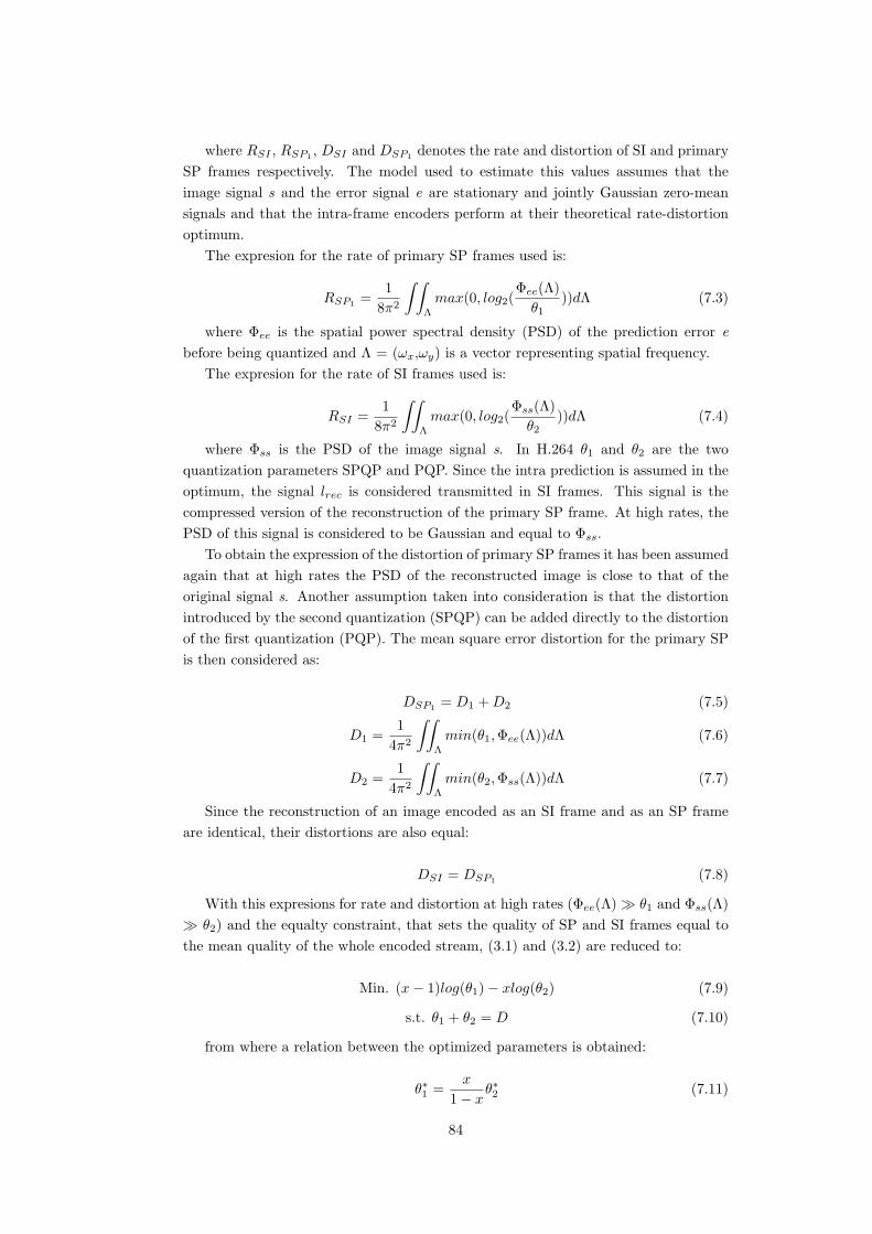
where RSI , RSP1 , DSI and DSP1 denotes the rate and distortion of SI and primarySP frames respectively. The model used to estimate this values assumes that theimage signal s and the error signal e are stationary and jointly Gaussian zero-meansignals and that the intra-frame encoders perform at their theoretical rate-distortionoptimum.

The expresion for the rate of primary SP frames used is:

RSP1 =1

8π2

∫ ∫Λ

max(0, log2(Φee(Λ)θ1

))dΛ (7.3)

where Φee is the spatial power spectral density (PSD) of the prediction error ebefore being quantized and Λ = (ωx,ωy) is a vector representing spatial frequency.

The expresion for the rate of SI frames used is:

RSI =1

8π2

∫∫Λ

max(0, log2(Φss(Λ)θ2

))dΛ (7.4)

where Φss is the PSD of the image signal s. In H.264 θ1 and θ2 are the twoquantization parameters SPQP and PQP. Since the intra prediction is assumed in theoptimum, the signal lrec is considered transmitted in SI frames. This signal is thecompressed version of the reconstruction of the primary SP frame. At high rates, thePSD of this signal is considered to be Gaussian and equal to Φss.

To obtain the expression of the distortion of primary SP frames it has been assumedagain that at high rates the PSD of the reconstructed image is close to that of theoriginal signal s. Another assumption taken into consideration is that the distortionintroduced by the second quantization (SPQP) can be added directly to the distortionof the first quantization (PQP). The mean square error distortion for the primary SPis then considered as:

DSP1 = D1 +D2 (7.5)

D1 =1

4π2

∫∫Λ

min(θ1,Φee(Λ))dΛ (7.6)

D2 =1

4π2

∫∫Λ

min(θ2,Φss(Λ))dΛ (7.7)

Since the reconstruction of an image encoded as an SI frame and as an SP frameare identical, their distortions are also equal:

DSI = DSP1 (7.8)

With this expresions for rate and distortion at high rates (Φee(Λ)� θ1 and Φss(Λ)� θ2) and the equalty constraint, that sets the quality of SP and SI frames equal tothe mean quality of the whole encoded stream, (3.1) and (3.2) are reduced to:

Min. (x− 1)log(θ1)− xlog(θ2) (7.9)

s.t. θ1 + θ2 = D (7.10)

from where a relation between the optimized parameters is obtained:

θ∗1 =x

1− xθ∗2 (7.11)

84

For any Gaussian signal with a continuous PSD, at high frequencies the slope ofthe rate-distiortion function is expressed:

dR

dD=

−12log(2)Θ

(7.12)

where Θ is in H.264 the quantization parameter that generates the rate-distortioncurve. From this equation it is possible to obtain the slope of the distortion-ratefunctions of the error signal emphe and the reconstructed signal in an SP before beingquantized by SPQP s:

dRe

dDe= −0.85 ∗ 2

P QP−123 (7.13)

dRs

dDs= −0.85 ∗ 2

SP QP−123 (7.14)

The optimal values of SPQP ∗ and PQP ∗ are resulted by combining (3.11),(3.13)and (3.14):

SPQP ∗ = PQP ∗ + 3log2(x

1− x) (7.15)

Since an assumption is to have the same qualtiy in SP frames as in other framesof the video stream, SPQP ∗ and PQP ∗ can not exceed the quantization parameterQP used to encode the P frames. The last restriction is that the three quantizationparameters must be integers. With all these constraints and equations the only pos-sible optimum values are shown in Table 7.1 , as well as the optimal values derivedempirically.

x model ≤ 0.2 ≥ 0.2 and ≤ 0.5 ≥ 0.5x empirical ≤ 0.1 ≥ 0.1 and ≤ 0.2 ≥ 0.2PQP QP - 1 QP - 2 QP - 3SPQP QP - 10 QP - 5 QP

Table 7.1: Optimal values for PQP and SPQP

85

APPENDIX B: Quantization

parameter analysis

Results from the analysis of the influence of the different quantization parameters (QP,PQP and SPQP) from FOREMAN video with QCIF resolution.

Figure 7.4: SNR(QP)with PQP = 26 and SPQP = 26

86

Figure 7.5: Size(QP)with PQP = 26 and SPQP = 26

Figure 7.6: SNR(QP)with PQP = 26 and SPQP = 26

87

Figure 7.7: Size(QP) with PQP = 26 and SPQP = 26

Figure 7.8: SNR(PQP) with QP = 26 and SPQP = 26

88

Figure 7.9: Size(PQP) with QP = 26 and SPQP = 26

Figure 7.10: SNR(PQP) with QP = 26 and SPQP = 26

89

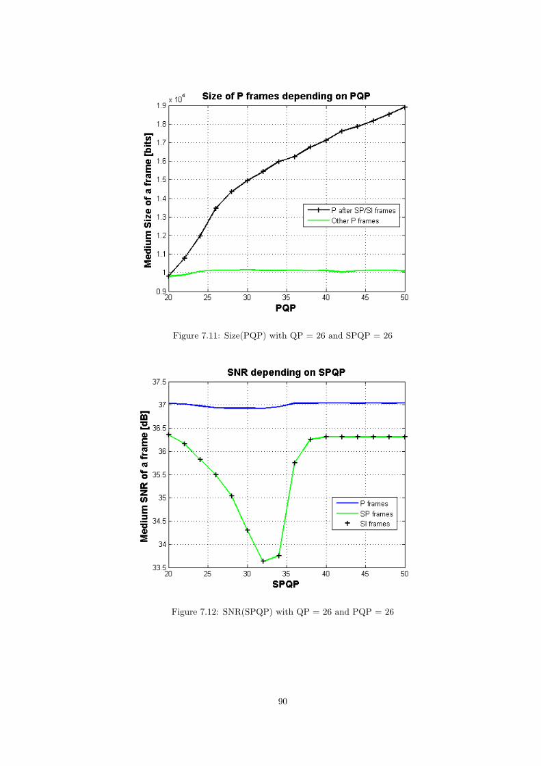
Figure 7.11: Size(PQP) with QP = 26 and SPQP = 26

Figure 7.12: SNR(SPQP) with QP = 26 and PQP = 26

90

Figure 7.13: Size(SPQP) with QP = 26 and PQP = 26

Figure 7.14: SNR(SPQP) with QP = 26 and PQP = 26

91

Figure 7.15: Size(SPQP) with QP = 26 and PQP = 26

Figure 7.16: Type of macroblocks in an SP frame depending on SPQP

92

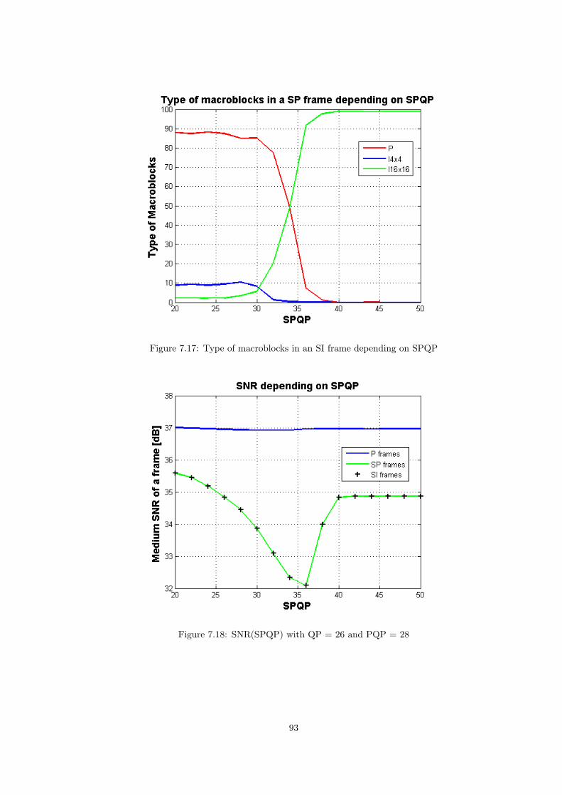
Figure 7.17: Type of macroblocks in an SI frame depending on SPQP

Figure 7.18: SNR(SPQP) with QP = 26 and PQP = 28

93

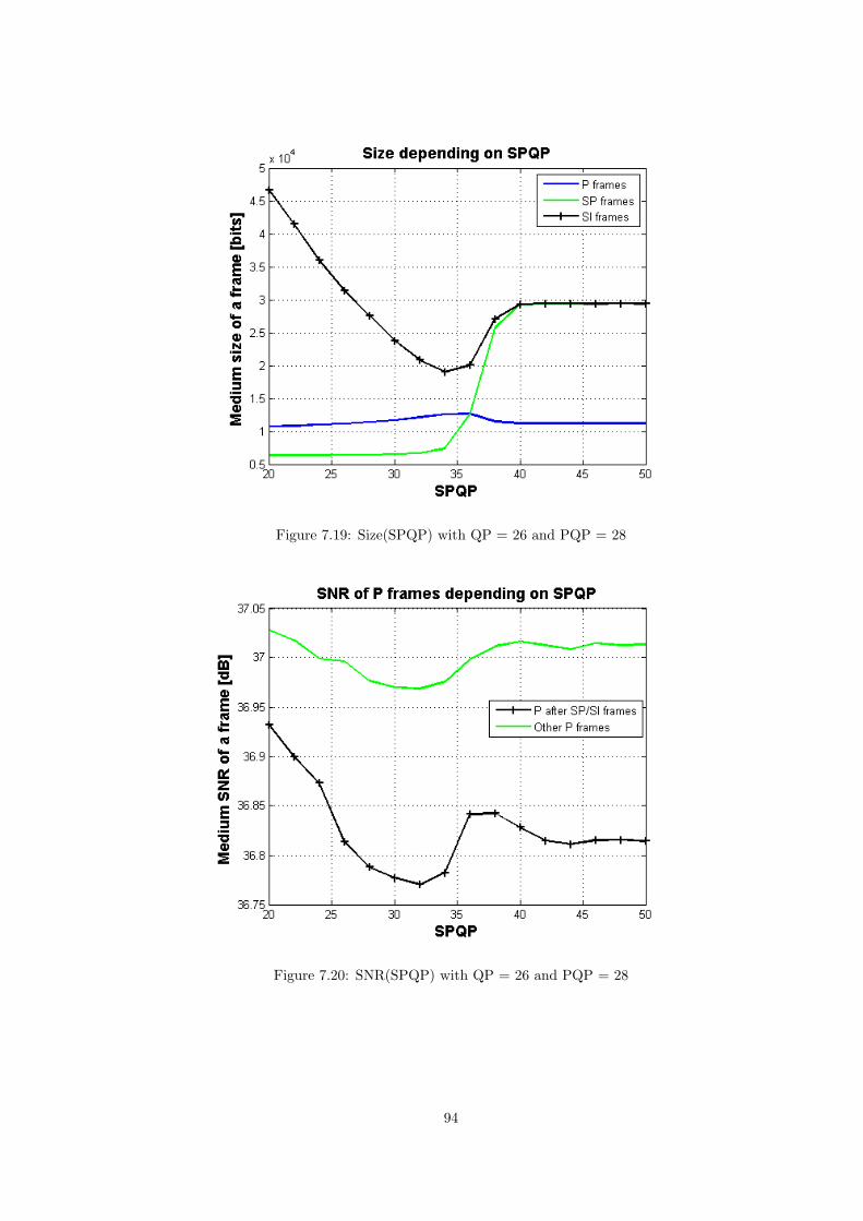
Figure 7.19: Size(SPQP) with QP = 26 and PQP = 28

Figure 7.20: SNR(SPQP) with QP = 26 and PQP = 28

94

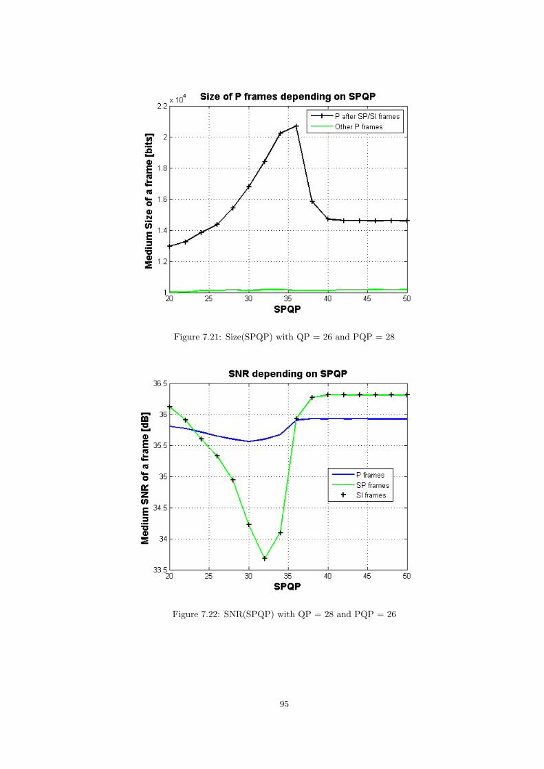
Figure 7.21: Size(SPQP) with QP = 26 and PQP = 28

Figure 7.22: SNR(SPQP) with QP = 28 and PQP = 26

95

Figure 7.23: Size(SPQP) with QP = 28 and PQP = 26

Figure 7.24: SNR(SPQP) with QP = 28 and PQP = 26

96

Figure 7.25: Size(SPQP)with QP = 28 and PQP = 26

97

APPENDIX C: Switching

Process analysis

Figure 7.26: Comparison of CIF and QCIF resolution in Foreman video.

98

Figure 7.27: Foreman QCIF - Encoding - Performance of different SP periods.

Figure 7.28: Foreman QCIF - Encoding - Performance of different GOPs.

99

Figure 7.29: Foreman QCIF - Encoding - Comparison of performance.

Figure 7.30: Foreman CIF - Decoding - SP Period equal to 5.

100

Figure 7.31: Foreman QCIF - Decoding - Feedback channel delay 100 ms.

Figure 7.32: Foreman QCIF - Decoding - Feedback channel delay 1500 ms.

101

Figure 7.33: Foreman QCIF - Decoding - SP Period equal to 5, different delays.

Figure 7.34: Foreman QCIF - Decoding - SP Period equal to 10, different delays.

102

Figure 7.35: Foreman CIF - Decoding - Delay 100 ms, Performance of different SPPeriods.

Figure 7.36: Foreman CIF - Decoding - Performance of different GOPs.

103

Figure 7.37: Foreman CIF - Decoding - Delay 100 ms, Performance SP/P and I/P.

Figure 7.38: Foreman CIF - GOP 7, quality degradation in transmission.

104

Figure 7.39: Foreman CIF - SP Period 7, delay 100 ms, quality degradation in trans-mission.

Figure 7.40: Foreman QCIF - Period 7, Efficiency comparison.

105

Figure 7.41: Foreman QCIF - Period 10, Efficiency comparison.

Figure 7.42: Mother and Daughter CIF - Period 7, Efficiency comparison.

106

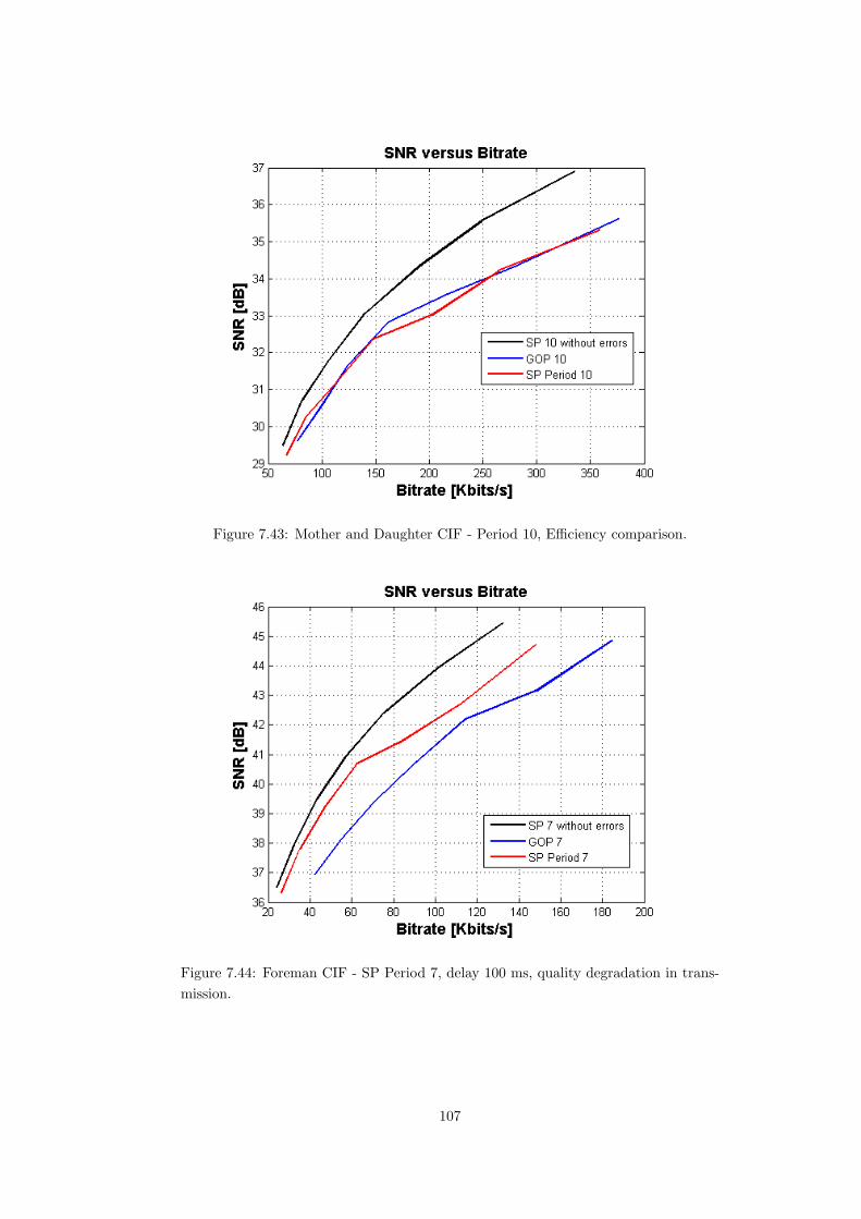
Figure 7.43: Mother and Daughter CIF - Period 10, Efficiency comparison.

Figure 7.44: Foreman CIF - SP Period 7, delay 100 ms, quality degradation in trans-mission.

107

Figure 7.45: Foreman CIF - SP Period 7, delay 100 ms, quality degradation in trans-mission.

108

APPENDIX D: Encoder’s

configuration file

The different features of the encoded sequence are decided in the configuration file.The types of frames in the bitstream is chosen by selecting the periodicity of I and SP.If it is a bitstream with only P and I frames, the SP periodicity is set to 0 and theGOP is set in the field IntraPeriod. In case of a bitstream with P and SP/SI frames,the value of the previous field must be 0 and the SP periodicity is set to the desiredvalue. If the bitstream is with SI frames instead of SP frames, SI FRAMES parametermust be 1. Another selectionable characteristics are the video to encode, its resolution,the profile of the encoder, the value of the different quantization parameters involved,which packetization to use, etcetera. In this project the packetization used is RTPpackets with fixed size of 700 bytes and the parameters to fixed are: OutFileMode,SliceMode and SliceArgument.

The identifiers used for the different quantization parameters used in the configu-ration file are:

• QP = QPISlice and QPPSlice because the same values is used in this projectfor the quatization parameter in I and P frames coincide.

• PQP = QPSPSlice

• SPQP = QPSP2Slice

It is shown below a configuration file with SP frames:

# <ParameterName >= <ParameterValue ># Comment## See configfile.h for a list of supported ParameterNames## For bug reporting and known issues see:# https://ipbt.hhi.de

############################################# Files############################################

InputFile = “mother daughter qcif.txt”# Input sequence

109

InputHeaderLength = 0 # If the inputfile has a header, state it is length in bytehere

StartFrame = 0 # Start frame for encoding. (0-N)FramesToBeEncoded = 100 # Number of frames to be codedFrameRate = 30.0 # Frame Rate per second (0.1-100.0)SourceWidth = 176 # Frame widthSourceHeight = 144 # Frame heightTraceFile = “trace enc.txt”ReconFile = “test recMOTHER DAUGHTER sp 5 17 16 7.yuv”OutputFile = “testMOTHER DAUGHTER sp 5 17 16 7.264”

############################################# Encoder Control############################################

ProfileIDC = 88 # Profile IDC (66=baseline, 77=main, 88=extended; FREXTProfiles: 100=High, 110=High 10, 122=High 4:2:2, 244=High 4:4:4, 44=CAVLC 4:4:4Intra)

LevelIDC = 40 # Level IDC (e.g. 20 = level 2.0)IntraPeriod = 0 # Period of I-pictures (0=only first)EnableOpenGOP = 0 # Support for open GOPs (0: disabled, 1: enabled)IDRIntraEnable = 0 # Force IDR Intra (0=disable 1=enable)QPISlice = 17 # Quant. param for I Slices (0-51)QPPSlice = 17 # Quant. param for P Slices (0-51)FrameSkip = 2 # Number of frames to be skipped in input (e.g 2 will code every

third frame)ChromaQPOffset = 0 # Chroma QP offset (-51..51)UseHadamard = 1 # Hadamard transform (0=not used, 1=used for all subpel

positions, 2=use only for qpel)DisableSubpelME = 0 # Disable Subpixel Motion Estimation (0=off/default, 1=on)SearchRange = 16 # Max search rangeNumberReferenceFrames = 1 # Number of previous frames used for inter motion

search (0-16)PList0References = 0 # P slice List 0 reference override (0 disable, N ¡= Number-

ReferenceFrames)Log2MaxFNumMinus4 = 0 # Sets log2 max frame num minus4 (-1 : based on

FramesToBeEncoded/Auto, ¿=0 :Log2MaxFNumMinus4)Log2MaxPOCLsbMinus4 = -1 # Sets log2 max pic order cnt lsb minus4 (-1 : Auto,

¿=0 : Log2MaxPOCLsbMinus4)GenerateMultiplePPS = 0 # Transmit multiple parameter sets. Currently param-

eters basically enable all WP modes (0: diabled, 1: enabled)ResendPPS = 0 # Resend PPS (with pic parameter set id 0) for every coded

Frame/Field pair (0: disabled, 1: enabled)

110

MbLineIntraUpdate = 0 # Error robustness(extra intra macro block updates)(0=off,N: One GOB every N frames are intra coded)

RandomIntraMBRefresh = 0 # Forced intra MBs per pictureInterSearch16x16 = 1 # Inter block search 16x16 (0=disable, 1=enable)InterSearch16x8 = 1 # Inter block search 16x8 (0=disable, 1=enable)InterSearch8x16 = 1 # Inter block search 8x16 (0=disable, 1=enable)InterSearch8x8 = 1 # Inter block search 8x8 (0=disable, 1=enable)InterSearch8x4 = 1 # Inter block search 8x4 (0=disable, 1=enable)InterSearch4x8 = 1 # Inter block search 4x8 (0=disable, 1=enable)InterSearch4x4 = 1 # Inter block search 4x4 (0=disable, 1=enable)IntraDisableInterOnly = 0 # Apply Disabling Intra conditions only to Inter Slices

(0:disable/default,1: enable)Intra4x4ParDisable = 0 # Disable Vertical & Horizontal 4x4Intra4x4DiagDisable = 0 # Disable Diagonal 45degree 4x4Intra4x4DirDisable = 0 # Disable Other Diagonal 4x4Intra16x16ParDisable = 0 # Disable Vertical & Horizontal 16x16Intra16x16PlaneDisable = 0 # Disable Planar 16x16ChromaIntraDisable = 0 # Disable Intra Chroma modes other than DCEnableIPCM = 1 # Enable IPCM macroblock modeDisposableP = 0 # Enable Disposable P slices in the primary layer (0: dis-

able/default, 1: enable)DispPQPOffset = 0 # Quantizer offset for disposable P slices (0: default)

############################################# B Slices############################################

NumberBFrames = 0 # Number of B coded frames inserted (0=not used)QPBSlice = 30 # Quant. param for B slices (0-51)BRefPicQPOffset = 0 # Quantization offset for reference B coded pictures (-51..51)DirectModeType = 1 # Direct Mode Type (0:Temporal 1:Spatial)DirectInferenceFlag = 1 # Direct Inference Flag (0: Disable 1: Enable)BList0References = 0 # B slice List 0 reference override (0 disable, N ¡= Number-

ReferenceFrames)BList1References = 1 # B slice List 1 reference override (0 disable, N ¡= Number-

ReferenceFrames)# 1 List1 reference is usually recommended for normal GOP Structures.# A larger value is usually more appropriate if a more flexible# structure is used (i.e. using HierarchicalCoding)BReferencePictures = 0 # Referenced B coded pictures (0=off, 1=B references for

secondary layer, 2=B references for primary layer)HierarchicalCoding = 0 # B hierarchical coding (0= off, 1= 2 layers, 2= 2 full

hierarchy, 3 = explicit)HierarchyLevelQPEnable = 1 # Adjust QP based on hierarchy level (in increments

of 1). Overrides BRefPicQPOffset behavior.(0=off, 1=on)

111

ExplicitHierarchyFormat = “b1r0b3r0b2e2b0e2b4r2”# Explicit Enhancement GOP.Format is FrameDisplay orderReferenceQP.

# Valid values for reference type is r:reference, e:non reference.ReferenceReorder = 1 # Reorder References according to Poc distance for Hierar-

chicalCoding (0=off, 1=enable)PocMemoryManagement = 1 # Memory management based on Poc Distances for

HierarchicalCoding (0=off, 1=on)BiPredMotionEstimation = 0 # Enable Bipredictive based Motion Estimation

(0:disabled, 1:enabled)BiPredMERefinements = 3 # Bipredictive ME extra refinements (0: single, N: N

extra refinements (1 default)BiPredMESearchRange = 16 # Bipredictive ME Search range (8 default). Note

that range is halved for every extra refinement.BiPredMESubPel = 1 # Bipredictive ME Subpixel Consideration (0: disabled, 1:

single level, 2: dual level)

############################################# SP Frames############################################

SPPicturePeriodicity = 5 # SP-Picture Periodicity (0=not used)QPSPSlice = 16 # Quant. param of SP-Slices for Prediction Error (0-51)QPSP2Slice = 7 # Quant. param of SP-Slices for Predicted Blocks (0-51)SI FRAMES = 0 # SI frame encoding flag (0=not used, 1=used)SP output = 0 # Controls whether coefficients will be output to encode switching

SP frames (0=no, 1=yes)SP output name = “low quality.dat”# Filename for SP output coefficientsSP2 FRAMES = 0 # switching SP frame encoding flag (0=not used, 1=used)SP2 input name1 = “high quality.dat”# Filename for the first swithed bitstream

coefficientsSP2 input name2 = “low quality.dat”# Filename for the second switched bit-

stream coefficients

############################################# Output Control, NALs############################################

SymbolMode = 0 # Symbol mode (Entropy coding method: 0=UVLC, 1=CABAC)OutFileMode = 1 # Output file mode, 0:Annex B, 1:RTPPartitionMode = 0 # Partition Mode, 0: no DP, 1: 3 Partitions per Slice

############################################# CABAC context initialization############################################

112

ContextInitMethod = 1 # Context init (0: fixed, 1: adaptive)FixedModelNumber = 0 # model number for fixed decision for inter slices ( 0, 1,

or 2 )

############################################# Interlace Handling############################################

PicInterlace = 0 # Picture AFF (0: frame coding, 1: field coding, 2:adaptiveframe/field coding)

MbInterlace = 0 # Macroblock AFF (0: frame coding, 1: field coding, 2:adaptiveframe/field coding, 3: frame MB-only AFF)

IntraBottom = 0 # Force Intra Bottom at GOP Period

############################################# Weighted Prediction############################################

WeightedPrediction = 0 # P picture Weighted Prediction (0=off, 1=explicit mode)WeightedBiprediction = 0 # B picture Weighted Prediciton (0=off, 1=explicit

mode, 2=implicit mode)UseWeightedReferenceME = 0 # Use weighted reference for ME (0=off, 1=on)

############################################# Picture based Multi-pass encoding############################################

RDPictureDecision = 0 # Perform RD optimal decision between different codedpicture versions.

# If GenerateMultiplePPS is enabled then this will test different WP methods.# Otherwise it will test QP +-1 (0: disabled, 1: enabled)RDPictureIntra = 0 # Perform RD optimal decision also for intra coded pictures

(0: disabled (default), 1: enabled).RDPSliceWeightOnly = 1 # Only consider Weighted Prediction for P slices in

Picture RD decision. (0: disabled, 1: enabled (default))RDBSliceWeightOnly = 0 # Only consider Weighted Prediction for B slices in

Picture RD decision. (0: disabled (default), 1: enabled )

############################################# Loop filter parameters############################################

LoopFilterParametersFlag = 0 # Configure loop filter (0=parameter below in-gored, 1=parameters sent)

LoopFilterDisable = 0 # Disable loop filter in slice header (0=Filter, 1=No Filter)LoopFilterAlphaC0Offset = 0 # Alpha & C0 offset div. 2, -6, -5, ... 0, +1, .. +6

113

LoopFilterBetaOffset = 0 # Beta offset div. 2, -6, -5, ... 0, +1, .. +6

############################################# Error Resilience / Slices############################################

SliceMode = 2 # Slice mode (0=off 1=fixed #mb in slice 2=fixed #bytes in slice3=use callback)

SliceArgument = 700 # Slice argument (Arguments to modes 1 and 2 above)num slice groups minus1 = 0 # Number of Slice Groups Minus 1, 0 == no FMO,

1 == two slice groups, etc.slice group map type = 0 # 0: Interleave, 1: Dispersed, 2: Foreground with left-

over,# 3: Box-out, 4: Raster Scan 5: Wipe# 6: Explicit, slice group id read from SliceGroupConfigFileNameslice group change direction flag = 0 # 0: box-out clockwise, raster scan or wipe

right,# 1: box-out counter clockwise, reverse raster scan or wipe leftslice group change rate minus1 = 85 #SliceGroupConfigFileName = “sg0conf.cfg”# Used for slice group map type 0, 2,

6UseRedundantPicture = 0 # 0: not used, 1: enabledNumRedundantHierarchy = 1 # 0-4PrimaryGOPLength = 10 # GOP length for redundant allocation (1-16)# NumberReferenceFrames must be no less than PrimaryGOPLength when redun-

dant slice enabledNumRefPrimary = 1 # Actually used number of references for primary slices (1-16)

############################################# Search Range Restriction / RD Optimization############################################

RestrictSearchRange = 2 # restriction for (0: blocks and ref, 1: ref, 2: no restric-tions)

RDOptimization = 1 # rd-optimized mode decision# 0: RD-off (Low complexity mode)# 1: RD-on (High complexity mode)# 2: RD-on (Fast high complexity mode - not work in FREX Profiles)# 3: with lossesDisableThresholding = 0 # Disable Thresholding of Transform Coefficients (0:off,

1:on)DisableBSkipRDO = 0 # Disable B Skip Mode consideration from RDO Mode

decision (0:off, 1:on)SkipIntraInInterSlices = 0 # Skips Intra mode checking in inter slices if certain

mode decisions are satisfied (0: off, 1: on)

114

# Explicit Lambda UsageUseExplicitLambdaParams = 0 # Use explicit lambda scaling parameters (0:dis-

abled, 1:enable lambda weight, 2: use explicit lambda value)LambdaWeightIslice = 0.65 # scaling param for I slices. This will be used as a

multiplier i.e.lambda=LambdaWeightISlice * 2((QP-12)/3)LambdaWeightPslice = 0.68 # scaling param for P slices. This will be used as a

multiplier i.e. lambda=LambdaWeightPSlice * 2((QP-12)/3)LambdaWeightBslice = 2.00 # scaling param for B slices. This will be used as a

multiplier i.e. lambda=LambdaWeightBSlice * 2((QP-12)/3)LambdaWeightRefBslice = 1.50 # scaling param for Referenced B slices. This will

be used as a multiplier i.e. lambda=LambdaWeightRefBSlice * 2((QP-12)/3)LambdaWeightSPslice = 1.50 # scaling param for SP slices. This will be used as

a multiplier i.e. lambda=LambdaWeightSPSlice * 2((QP-12)/3)LambdaWeightSIslice = 0.65 # scaling param for SI slices. This will be used as a

multiplier i.e. lambda=LambdaWeightSISlice * 2((QP-12)/3)LossRateA = 5 # expected packet loss rate of the channel for the first partition,

only valid if RDOptimization = 3LossRateB = 0 # expected packet loss rate of the channel for the second partition,

only valid if RDOptimization = 3LossRateC = 0 # expected packet loss rate of the channel for the third partition,

only valid if RDOptimization = 3NumberOfDecoders = 30 # Numbers of decoders used to simulate the channel,

only valid if RDOptimization = 3RestrictRefFrames = 0 # Doesnt allow reference to areas that have been intra

updated in a later frame.

############################################# Additional Stuff############################################

UseConstrainedIntraPred = 0 # If 1, Inter pixels are not used for Intra macroblockprediction.

LastFrameNumber = 0 # Last frame number that have to be coded (0: no effect)ChangeQPI = 16 # QP (I-slices) for second part of sequence (0-51)ChangeQPP = 16 # QP (P-slices) for second part of sequence (0-51)ChangeQPB = 18 # QP (B-slices) for second part of sequence (0-51)ChangeQPBSRefOffset = 2 # QP offset (stored B-slices) for second part of se-

quence (-51..51)ChangeQPStart = 0 # Frame no. for second part of sequence (0: no second part)NumberofLeakyBuckets = 8 # Number of Leaky Bucket valuesLeakyBucketRateFile = “leakybucketrate.cfg”# File from which encoder derives

rate valuesLeakyBucketParamFile = “leakybucketparam.cfg”# File where encoder stores leaky-

bucketparams

115

NumberFramesInEnhancementLayerSubSequence = 0 # number of frames in theEnhanced Scalability Layer(0: no Enhanced Layer)

SparePictureOption = 0 # (0: no spare picture info, 1: spare picture available)SparePictureDetectionThr = 6 # Threshold for spare reference pictures detectionSparePicturePercentageThr = 92 # Threshold for the spare macroblock percentagePicOrderCntType = 0 # (0: POC mode 0, 1: POC mode 1, 2: POC mode 2)

############################################# Rate control############################################

RateControlEnable = 0 # 0 Disable, 1 EnableBitrate = 45020 # Bitrate(bps)InitialQP = 0 # Initial Quantization Parameter for the first I frame# InitialQp depends on two values: Bits Per Picture,# and the GOP lengthBasicUnit = 11 # Number of MBs in the basic unit# should be a fractor of the total number# of MBs in a frameChannelType = 0 # type of channel( 1=time varying channel; 0=Constant chan-

nel)

############################################# Fast Mode Decision############################################

EarlySkipEnable = 0 # Early skip detection (0: Disable 1: Enable)SelectiveIntraEnable = 0 # Selective Intra mode decision (0: Disable 1: Enable)

############################################# FREXT stuff############################################

YUVFormat = 1 # YUV format (0=4:0:0, 1=4:2:0, 2=4:2:2, 3=4:4:4)RGBInput = 0 # 1=RGB input, 0=GBR or YUV inputBitDepthLuma = 8 # Bit Depth for Luminance (8...12 bits)BitDepthChroma = 8 # Bit Depth for Chrominance (8...12 bits)CbQPOffset = 0 # Chroma QP offset for Cb-part (-51..51)CrQPOffset = 0 # Chroma QP offset for Cr-part (-51..51)Transform8x8Mode = 0 # (0: only 4x4 transform, 1: allow using 8x8 transform

additionally, 2: only 8x8 transform)ReportFrameStats = 0 # (0:Disable Frame Statistics 1: Enable)DisplayEncParams = 0 # (0:Disable Display of Encoder Params 1: Enable)Verbose = 1 # level of display verboseness (0:short, 1:normal, 2:detailed)

116

############################################# Q-Matrix (FREXT)############################################

QmatrixFile = “q matrix.cfg”ScalingMatrixPresentFlag = 0 # Enable Q Matrix (0 Not present, 1 Present in

SPS, 2 Present in PPS, 3 Present in both SPS & PPS)ScalingListPresentFlag0 = 3 # Intra4x4 Luma (0 Not present, 1 Present in SPS,

2 Present in PPS, 3 Present in both SPS & PPS)ScalingListPresentFlag1 = 3 # Intra4x4 ChromaU (0 Not present, 1 Present in

SPS, 2 Present in PPS, 3 Present in both SPS & PPS)ScalingListPresentFlag2 = 3 # Intra4x4 chromaV (0 Not present, 1 Present in

SPS, 2 Present in PPS, 3 Present in both SPS & PPS)ScalingListPresentFlag3 = 3 # Inter4x4 Luma (0 Not present, 1 Present in SPS,

2 Present in PPS, 3 Present in both SPS & PPS)ScalingListPresentFlag4 = 3 # Inter4x4 ChromaU (0 Not present, 1 Present in

SPS, 2 Present in PPS, 3 Present in both SPS & PPS)ScalingListPresentFlag5 = 3 # Inter4x4 ChromaV (0 Not present, 1 Present in

SPS, 2 Present in PPS, 3 Present in both SPS & PPS)ScalingListPresentFlag6 = 3 # Intra8x8 Luma (0 Not present, 1 Present in SPS,

2 Present in PPS, 3 Present in both SPS & PPS)ScalingListPresentFlag7 = 3 # Inter8x8 Luma (0 Not present, 1 Present in SPS,

2 Present in PPS, 3 Present in both SPS & PPS)

############################################# Rounding Offset control############################################

OffsetMatrixPresentFlag = 0 # Enable Explicit Offset Quantization Matrices (0:disable 1: enable)

QOffsetMatrixFile = “q offset.cfg”# Explicit Quantization Matrices fileAdaptiveRounding = 0 # Enable Adaptive Rounding based on JVT-N011 (0: dis-

able, 1: enable)AdaptRndPeriod = 1 # Period in terms of MBs for updating rounding offsets.# 0 performs update at the picture level. Default is 16. 1 is as in JVT-N011.AdaptRndChroma = 0 # Enables coefficient rounding adaptation for chromaAdaptRndWFactorIRef = 4 # Adaptive Rounding Weight for I/SI slices in refer-

ence pictures /4096AdaptRndWFactorPRef = 4 # Adaptive Rounding Weight for P/SP slices in ref-

erence pictures /4096AdaptRndWFactorBRef = 4 # Adaptive Rounding Weight for B slices in reference

pictures /4096AdaptRndWFactorINRef = 4 # Adaptive Rounding Weight for I/SI slices in non

reference pictures /4096

117

AdaptRndWFactorPNRef = 4 # Adaptive Rounding Weight for P/SP slices innon reference pictures /4096

AdaptRndWFactorBNRef = 4 # Adaptive Rounding Weight for B slices in nonreference pictures /4096

############################################# Lossless Coding (FREXT)############################################

QPPrimeYZeroTransformBypassFlag = 0 # Enable lossless coding when qpprime yis zero (0 Disabled, 1 Enabled)

############################################# Fast Motion Estimation Control Parameters############################################

UseFME = 0 # Use fast motion estimation (0=disable/default, 1=UMHexagonS# 2=Simplified UMHexagonS, 3=EPZS patterns)FMEDSR = 1 # Use Search Range Prediction. Only for UMHexagonS method# (0:disable, 1:enabled/default)FMEScale = 3 # Use Scale factor for different image sizes. Only for UMHexagonS

method# (0:disable, 3:/default)# Increasing value can speed up Motion Search.EPZSPattern = 2 # Select EPZS primary refinement pattern.# (0: small diamond, 1: square, 2: extended diamond/default,# 3: large diamond, 4: SBP Large Diamond,# 5: PMVFAST )EPZSDualRefinement = 3 # Enables secondary refinement pattern.# (0:disabled, 1: small diamond, 2: square,# 3: extended diamond/default, 4: large diamond,# 5: SBP Large Diamond, 6: PMVFAST )EPZSFixedPredictors = 2 # Enables Window based predictors# (0:disabled, 1: P only, 2: P and B/default)EPZSTemporal = 1 # Enables temporal predictors# (0: disabled, 1: enabled/default)EPZSSpatialMem = 1 # Enables spatial memory predictors# (0: disabled, 1: enabled/default)EPZSMinThresScale = 0 # Scaler for EPZS minimum threshold (0 default).# Increasing value can speed up encoding.EPZSMedThresScale = 1 # Scaler for EPZS median threshold (1 default).# Increasing value can speed up encoding.EPZSMaxThresScale = 1 # Scaler for EPZS maximum threshold (1 default).# Increasing value can speed up encoding.

118

APPENDIX E: Decoder’s

configuration file

Example of a configuration file of the decoder:

mezcla 5 17 100 50.txt ........H.26L coded bitstreamdecoder video.yuv ........Output file, YUV/RGBmother daughter qcif.txt ........Ref sequence (for SNR)1 ........Write 4:2:0 chroma components for monochrome streams1 ........NAL mode (0=Annex B, 1: RTP packets)0 ........SNR computation offset2 ........Poc Scale (1 or 2)500000 ........Rate Decoder104000 ........B decoder73000 ........F decoderleakybucketparam.cfg ........LeakyBucket Params1 ........Err Concealment(0:Off,1:Frame Copy,2:Motion Copy)4 ........Reference POC gap (2: IPP (Default), 4: IbP / IpP)4 ........POC gap (2: IPP /IbP/IpP (Default), 4: IPP with frame skip = 1 etc.)

This is a file containing input parameters to the JVT H.264/AVC decoder.The text line following each parameter is discarded by the decoder.

119