application of principal component analysis-assisted

Research ArticleApplication of Principal Component Analysis-Assisted NeuralNetworks for the Rotor Blade Load Prediction

Jiahong Zheng ,1 Shuaike Jiao,1 and Ding Cui2

1Institute of Flight Test Technology, Chinese Flight Test Establishment, Xi’an 710089, China2Institute of Applied Electronics, China Academy of Engineering Physics, Mianyang 621900, China

Correspondence should be addressed to Jiahong Zheng; [email protected]

Received 16 January 2021; Revised 5 April 2021; Accepted 13 May 2021; Published 24 May 2021

Academic Editor: Zhiguang Song

Copyright © 2021 Jiahong Zheng et al. This is an open access article distributed under the Creative Commons Attribution License,which permits unrestricted use, distribution, and reproduction in any medium, provided the original work is properly cited.

This paper presents a novel approach of principal component analysis- (PCA-) assisted back propagation (BP) neural networks forthe problem of rotor blade load prediction. 86.5 hours of real flight data were collected from many steady-state and transient flightmaneuvers at different altitudes and airspeeds. Prediction of the blade loads was determined by the PCA-BP model from 16 flightparameters measured and monitored by the flight control computer already present in the helicopter. PCA was applied to reducethe dimension of the flight parameters influencing the component load and eliminate the correlation among flight parameters.Thus, obtained principal components were used as input vectors of the BP neural network. The combined PCA-BP neuralnetwork model was trained and tested by real flight data. Comparison of this model and to a BP neural network model as wellas to a multiple linear regression (MLR) model was also done. The results of comparison demonstrate that the PCA-BP modelhas higher prediction precision with an average error of 2.46%, while 4.49% for BP and 10.20% for MLR. The results also revealthat the PCA-BP model has a shorter convergence path than the BP model. This method not only is useful in establishing theload spectra of helicopter rotor in-service where installation of strain gauges is impractical but also can reduce the cost ofinstallation and maintenance measured by strain gauges.

1. Introduction

The fatigue life of helicopter structures plays an essential rolein helicopter-maintenance work, as components of a helicop-ter could be fatigue-damaged under various working condi-tions with loads. Reliable measurement and prediction offatigue damage then would be the key for timely replacementof necessary components and comply to the Strength Regula-tions for Military Helicopters. The common practice indetermining the fatigue life applies the Palmgren-Minercumulative damage theory, where one takes the loads indifferent maneuvers as input data [1–3].

A common method of obtaining the component loads isto directly measure by installing strain gauges. Although thismethod is able to get a high accuracy for component loads,this way will bring some disadvantages. Firstly, this can beexpensive considering installation and maintenance costs[2]. Secondly, it is often impractical because strain gaugesnormally cannot be mounted on an in-service helicopter

[4]. Besides, the installation of strain gauges would lead tothe occupation of helicopter space [5]. In addition, it oftentakes more than one year to collect data and needs a longtime analysis as the load spectrum involves a series of flightmaneuvers [6].

Some researchers try to predict component loads by amathematical model and an intelligent model actively. Amathematical model is an important method for the predic-tion of rotor blade loads. However, the variables and thecomponent loads are intertwined in such a complex way thatcurrently, a precise mathematical model is still not anoption [7]. Therefore, many studies have proposed to pre-dict component loads by using an intelligence model thatcan model the complex relationship for improving theprediction precision. For example, prediction of the com-ponent loads is determined by a linear regression or neu-ral network model from the roll, pitch, airspeed, and otherflight parameters measured by the flight control computeron the helicopter [8].

HindawiInternational Journal of Aerospace EngineeringVolume 2021, Article ID 5594102, 13 pageshttps://doi.org/10.1155/2021/5594102

https://orcid.org/0000-0003-0923-9432

https://creativecommons.org/licenses/by/4.0/

https://creativecommons.org/licenses/by/4.0/

https://doi.org/10.1155/2021/5594102

Cabell et al. predicted oscillatory loads using a neural net-work for on-line health monitoring of flight essential compo-nents in an AH-64A helicopter. The linear model was alsoused to predict the load, and its accuracy was obviously lowerthan that of the neural network, especially at higher loadvalues that cause fatigue damage [9]. Haas et al. used a morecomplex method to model the load model derivation of thehelicopter rotor system. Both linear regression and neuralnetworks were used to create load models. Nonlinear effectswere found in the data and explained using a linear modelwith derived parameters created by a nonlinear mappingfunction or using a neural network model [10]. Allen andDibley applied neural networks to model the wing loads ofaircrafts. The linear model was established first as the startingpoint of the network training, which improved the accuracyof the neural network model [11]. Gómez-Escalonilla et al.developed a parametric full-scale fatigue monitoring systemfor an Airbus A330 using an artificial neural network withseveral strain gauges installed on some areas of the wingsand fuselage [4]. Cooper and DiMaio predicted the static loadon a wing rib of aircraft using an artificial neural network.This was achieved by using strain values obtained from thestatic test as an input parameter [7]. Elshafey et al. researchedon the use of neural networks to predict structural responseon structures [12]. De Paula et al. predicted nonlinearunsteady aerodynamic loads for NACA0012 airfoil usingneural networks [13].

Despite insufficient accuracy in the fatigue damageestimation, in these papers, encouraging progress has beenmade. However, the methods developed in these papersare rather inflexible for generalization when one attemptsto feed the neural network with the influencing factorsdirectly. One way to solve this problem is to preprocessthe data with the principal component analysis (PCA)method. The original data of the influencing factors is verylikely intercorrelated and possibly redundant. PCA isdesigned to reduce the data to the most compact andindependent sets while retaining the data’s information.Compared to the original data, data processed with PCAmitigates the demand of the complexity in the neural net-work. In this paper, a combination of PCA and the backpropagation (BP) neural network method was experimen-ted and compared to the pure BP method, as well as tomultilinear regression (MLR). The results show evidentenhancement in the accuracy of fatigue-damage estimationby the combined method of BP with PCA.

2. PCA and BP Neural Network Structure

2.1. Principal Component Analysis. The principal componentanalysis is a data-dimension-reduction technique. Construct-ing an appropriate set of linear combinations of the originalindicators, a series of unrelated comprehensive indicatorsare produced, from which a few comprehensive indicatorsare selected such that they contain as much information con-tained in the original indicators as possible. Thus, it is possi-ble to use fewer indicators to explain most of the variations inthe original data [14].

Suppose a data set has n samples, each expressed by anm-dimensional transposed vector, (x1, x2,⋯, xm), so theoriginal data matrix can be represented by an n ×m matrixX = ðxijÞn×m, with each row representing a sample. ThePCA consists of the following steps, which are shown inRef. [15–18].

2.1.1. Normalization of Raw Data. The original variablesneed to be standardized to eliminate the influence of differentdimensions, and it can be done according to the followingtwo equations:

�xij =xij −min x∗j

� �max x∗j

� �−min x∗j

� � , i = 1, 2,⋯,n, j = 1, 2,⋯,mð Þ,

ð1Þ

where min ðx∗jÞ stands for the smallest number of the nentries of the jth column in the matrix X. The logic behindthis choice is that the numbers in the same column quantifythe same characteristic feature. Equivalently, we can write theabove equation in a more compact form,

�x∗j =x∗j − min x∗j

� �� n

max x∗j� �

−min x∗j� � , j = 1, 2,⋯,mð Þ, ð2Þ

where ðmin ðx∗jÞÞn represents a vector with n entries whichare all equal to min ðx∗jÞ.2.1.2. Calculate the Correlation Coefficient Matrix R. The cor-relation coefficient matrix R can be calculated according tothe following specification:

R = rsq� �

m×m: ð3Þ

With the standard definition for correlation between twosets of data

rpq =1

σ �x∗sð Þσ �x∗q� �〠n

k=1�x∗s −mean �x∗sð Þð Þ

� �xkq −mean �x∗q� ��

s, q = 1, 2,⋯mð Þ,ð4Þ

where σð�x∗sÞ and meanð�x∗sÞ stand for the variance andaverage of the data, respectively. It is noted that rss = 1 andrsq = rqs.

2.1.3. Calculate the Eigenvalues and Feature Vector. Calculatethe eigenvalues λiði = 1, 2,⋯,mÞ of matrix R and arrangethem by size, namely, λ1 ≥ λ2 ≥⋯≥λm ≥ 0. Then, the featurevectors ui are just the eigenvectors of the eigenvalues λi.Specifically,

R ⋅ ui = λi ⋅ ui: ð5Þ

2 International Journal of Aerospace Engineering

In case of degeneracy, we assume that all real eigenvec-tors can still be found. Principal components can then beexpressed in terms of

F1 = u11 �x1 + u21 �x2+⋯+um1 �xm,F2 = u12 �x1 + u22 �x2+⋯+um2 �xm,⋯⋯

Fm = u1m �x1 + u2m �x2+⋯+umm �xm,

8>>>>><>>>>>:

ð6Þ

where F1 denotes the first principal components, F2 thesecond principal components, and Fm the mth principalcomponents.

2.1.4. Extract p Principal Components. First, the principalcomponent contribution rate and cumulative contributionrate are computed. Then, p principal components based onthe cumulative contribution rate are extracted. Calculate,respectively, the contribution rate bj of the jth principal com-ponent and the cumulative contribution rate ap by

bj =λj

∑mk=1λk

, j = 1, 2,⋯,mð Þ, ð7Þ

ap =∑p

k=1λk∑m

k=1λk: ð8Þ

The 1st, 2nd,…, pth ðp ≤mÞ principal components aretaken, when the contribution rates of the characteristic valueap reach up to 90%. Finally, the p principal components ofthe original samples can be expressed as in

yk = u1k �x1 + u2k �x2+⋯+umk�xm k = 1, 2,⋯pð Þ: ð9Þ

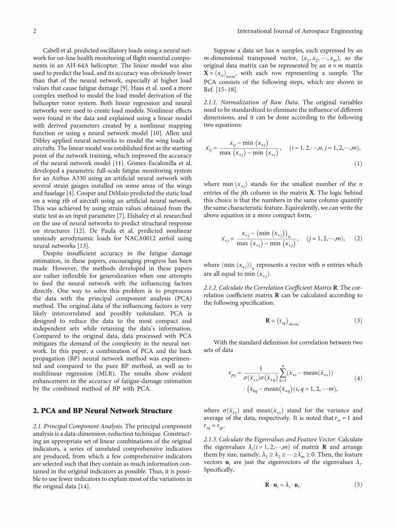
2.2. BP Neural Network. The BP is a popular technique ofneural networks for supervised learning. Its general structureis depicted in Figure 1.

As shown in Figure 1, there are three layers in a BPmodel, which are the input layer, hidden layer, and outputlayer. Two nodes of each adjacent layer are connecteddirectly, and it is called a link. Each link has a weighted valuerepresenting the degree of relationship between the twonodes. Suppose there are n input neurons,m hidden neurons,and one output neuron. A training process can be dividedinto two steps.

2.2.1. Hidden Layer Stage. Calculate the outputs of all neu-rons in the hidden layer according to the following steps:

netj = 〠n

i=0vijxi j = 1, 2,⋯,m, ð10Þ

yj = f H netj� �

j = 1, 2,⋯,m, ð11Þ

where vij is the weighted value from the ith neuron node inthe input layer to the jth node in the hidden layer, netj isthe activation value of the jth node, yj is the output of thehidden layer, and f H is the activation function of a node. Asigmoid function is usually expressed by formula (11):

f H xð Þ = 11 + exp −xð Þ : ð12Þ

2.2.2. Output Stage. The outputs of all neurons in the outputlayer is calculated in

o = f o 〠m

j=0ωjkyj

!, ð13Þ

X1 y1

Input layer Hidden layer Output layer

X2

Xn

y2

ym

Figure 1: Structure of BP neural network.

Weight

Rotor blade

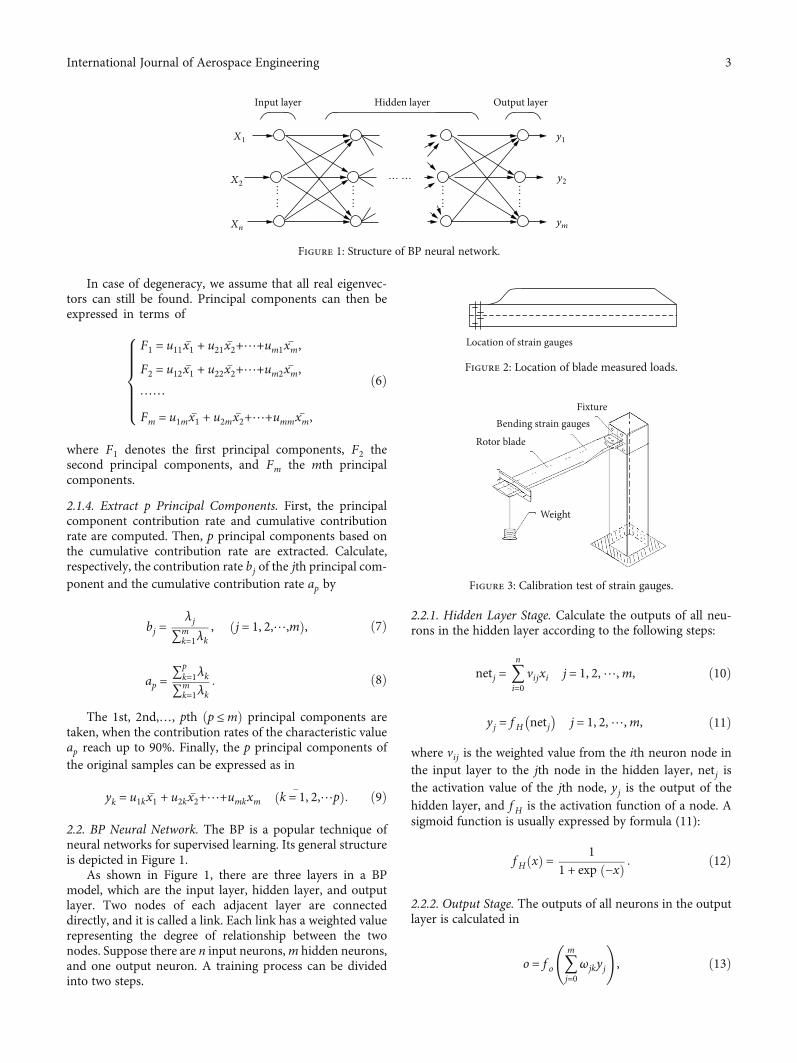
Bending strain gaugesFixture

Figure 3: Calibration test of strain gauges.

Location of strain gauges

Figure 2: Location of blade measured loads.

3International Journal of Aerospace Engineering

where ωjk is the weighted value from the jth neuron node inthe hidden layer to the pth node in the output layer and f o isthe activation function, and it is a linear function generally.All weights are assigned with random values initially. Theyare modified according to the learning samples traditionallyby the delta rule [19–22].

3. Math Experimental Data

The flight load data and flight parameter data were collectedby a specially instrumented helicopter. Rotor blade load datawith the root position were collected through the use of straingauges. The location of the strain gauges in the blade isshown in Figure 2. These strain gauges are temperature com-pensated to consider the expected temperature changes withaltitude, and there is a special coating on the strain gauge toprovide mechanical and environmental protection.

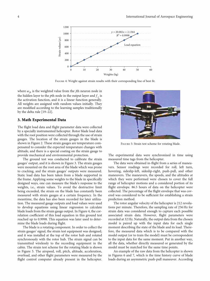
The ground test was conducted to calibrate the straingauges’ output, and it is shown in Figure 3. The strain gaugeswere mounted on the root area of the blade which was proneto cracking, and the strain gauges’ outputs were measured.Static load data has been taken from a blade supported inthe frame. Applying some weights to the blade in specificallydesigned ways, one can measure the blade’s response to theweights, i.e., strain values. To avoid the destructive limitbeing exceeded, the strain on the blade has constantly beenmeasured with strain gauges at a certain frequency. In themeantime, the data has also been recorded for later utiliza-tion. The measured gauge outputs and load values were usedto develop equations using linear regression to calculateblade loads from the strain gauge output. In Figure 4, the cor-relation coefficient of this load equation in this ground testreached up to 0.9998. This equation was later used to deter-mine the blade loads during flight.

The blade is a rotating component. In order to collect thestrain gauges’ signal, the strain test equipment was designed,and it was installed at the top of the rotor hub and rotatedsynchronously with the rotor hub. The strain signal can betransmitted wirelessly to the recording equipment in thecabin. The strain test scheme for the rotating blade is shownin Figure 5. The airspeed, roll, pitch, altitude, acceleration,overload, and other flight parameters were measured by theflight control computer already present in the helicopter.

The experimental data were synchronized in time usingmeasured time tags from the helicopter.

The data were obtained in-flight from a series of maneu-vers. Sensor readings were recorded for roll, left turn,hovering, sideslip-left, sideslip-right, push-pull, and othermaneuvers. The maneuvers, the speeds, and the altitudes atwhich they were performed were chosen to cover the fullrange of helicopter motions and a considered portion of itsflight envelope. 86.5 hours of data on the helicopter werecollected. The percentage of the flight envelope that was cov-ered was considered to be sufficient for establishing a strainprediction method.

The rotor angular velocity of the helicopter is 212 revolu-tions per minute. Therefore, the sampling rate of 256Hz forstrain data was considered enough to capture each possibleassociated strain data. However, flight parameters wererecorded at 32Hz. Naturally, the output data from the chosenmodel is paired up with the input data for each singlemoment describing the state of the blade and its load. There-fore, the measured data which is to be compared with themodel output (or to train the model) must be correspondentto the input data for the same moment. Put in another way,all the data, whether directly measured or generated by themodel must be matched for the same time points.

An example of the raw data from the helicopter is shownin Figures 6 and 7, which is the time history curve of bladeloads during an asymmetric push-pull maneuver. According

y = 20.002x + 2.1364 R² = 0.9998

0

200

400

600

800

1000

1200

0 10 20 30 40 50 60

Stra

in v

alue

s (𝜇𝜀)

Weights (kg)

Load equation

Figure 4: Weight against strain results with their corresponding line of best fit.

Figure 5: Strain test scheme for rotating blade.


to the Figure 6, we can see that the waveform is smooth, peri-odic, and without data spikes. When a helicopter performs asteady flight maneuver, the aerodynamic load of the bladechanges periodically with the azimuth of the rotor blade.Therefore, the load-time curve of the blade shows a periodictrend. The rotor angular velocity is 212 revolutions per min-ute, so the rotor rotates 3.53 laps in one second. We can seethat blade load data in a hovering maneuver were periodicalwaves corresponding to the rotor shaft’s rotation rate, which

is consistent with the theoretical analysis, while the loadwaveform during a symmetric push-pull maneuver inFigure 7 changed with the flight parameters. The time historycurves of some flight parameter data were shown in Figures 7and 8. Those waveforms were smooth and show no dataspikes. Therefore, it satisfies the model’s requirements forvariables because data spikes, noisy data, or invalid datamay lead to abnormal training of neural networks, thus hin-dering the generalizability of models. They are only a small

Flapping load

10:9:40:990 10:9:41:576 10:9:42:162 10:9:42:748

Flap

ping

load

(N·m

)

Time

Figure 7: Load-time curve during a symmetric push-pull maneuver.

Time

One period

11:29:40:999

Flap

ping

load

(N·m

)

Flapping load

11:29:41:499 11:29:41:999 11:29:42:499

Figure 6: Load-time curve during a hovering maneuver.


part of flight test data of the helicopter, which were used tocreate the prediction load models.

86.5 hours of flight data were arbitrarily divided intotraining data and test data, accounting for up to about 98%and 2%, respectively. It should be noted that training dataand test data were recorded on two different days to providediffering flight conditions, which can determine how general-

izable the models are and whether it can work in significantlydifferent operating circumstances.

4. Establishment of Model

4.1. Selection of Input and Output Variables. The selection ofthe input and output variables of the model is crucial as it

Table 1: Description of input variables.

Variables Minimum Maximum Units Symbol

Height 0 5500 m X1

Indicated airspeed 0 240 km/h X2

Collective pitch position 0 100 % X3

Longitudinal cyclic pitch position -180 180 mm X4

Lateral cyclic pitch position -180 180 mm X5

Pedal position -180 180 mm X6

Pitch angle -30 30 (°) X7

Roll angle -45 45 (°) X8

Angle of yaw 0 360 (°) X9

Pitch rate -30 30 °/s X10

Roll rate -30 30 °/s X11

Yaw rate -30 30 °/s X12

Normal acceleration 0.5 2.5 g X13

First engine torque 0 100 % X14

Second engine torque 0 100 % X15

Third engine torque 0 100 % X16

Flapping loads — — N·m Z

10:09:28:952 10:09:33:953 10:09:38:953 10:09:43:953

Val

ue o

f flig

ht v

aria

bles

(mm

)

Time

Collective pitch positionLongitudinal cyclic pitch position

Lateral cyclic pitch positionPedal position

Figure 8: Manipulation parameter-time curves during a push-pull maneuver.


directly affects the prediction accuracy of the rotor blade loadmodel. For the load model of the rotor blade, the output var-iable is the loads of the rotor blade, and the input variablesare determined by flight parameters. 16 flight parameterswere chosen as inputs to the model. These 16 flight parame-ters were selected because they can describe the status of thehelicopter during flight. In addition, they are monitored andrecorded by the flight control computer on the helicopter.Therefore, a flight load prediction system using these vari-

ables is convenient to be implemented by tapping into exist-ing data based on the helicopter. There is height, indicatedairspeed, collective pitch position, longitudinal cyclic pitchposition, lateral cyclic pitch position, pedal position, pitchangle, roll angle, angle of yaw, pitch rate, roll rate, yaw rate,normal acceleration, first engine torque, second engine tor-que, and third engine torque. These 16 variables, as well astheir minimum, maximum, units, and symbols are shownin Table 1.

Table 2: Correlation analysis of the process variables.

x1 x2 x3 x4 x5 x6 x7 x8 x9 x10 x11 x12 x13 x14 x15 x16x1 1.00 — — — — — — — — — — — — — — —

x2 -0.46 1.00 — — — — — — — — — — — — — —

x3 0.42 -0.40 1.00 — — — — — — — — — — — — —

x4 -0.77 0.54 -0.77 1.00 — — — — — — — — — — — —

x5 -0.71 0.55 0.90 0.93 1.00 — — — — — — — — — — —

x6 -0.09 -0.23 0.65 0.34 -0.49 1.00 — — — — — — — — — —

x7 -0.50 0.12 0.25 -0.13 0.08 0.69 1.00 — — — — — — — — —

x8 -0.43 0.23 0.91 0.79 0.91 -0.65 -0.31 1.00 — — — — — — — —

x9 0.65 -0.47 0.35 -0.48 -0.54 0.02 -0.32 0.34 1.00 — — — — — — —

x10 0.41 -0.85 -0.22 -0.55 -0.43 0.20 0.00 -0.34 0.37 1.00 — — — — — —

x11 -0.25 -0.33 -0.33 -0.66 0.13 0.34 0.49 0.21 0.00 -0.05 1.00 — — — — —

x12 0.49 -0.53 0.49 -0.52 0.67 -0.45 -0.19 0.44 0.79 -0.50 0.01 1.00 — — — —

x13 -0.50 0.35 -0.32 0.71 0.54 -0.21 0.38 -0.29 0.60 0.55 0.32 0.89 1.00 — — —

x14 -0.61 -0.57 -0.99 0.70 -0.62 -0.21 -0.34 0.45 -0.78 0.49 -0.21 -0.90 0.93 1.00 — —

x15 -0.59 0.42 -0.34 -0.65 0.56 0.18 -0.37 -0.42 -0.88 0.60 0.33 -0.90 0.99 0.99 1.00 —

x16 0.53 0.59 0.37 -0.34 0.49 0.20 0.13 0.28 0.60 0.44 -0.04 -0.64 0.46 -0.58 -0.45 1.00

Z -0.51 0.48 -0.50 -0.30 -0.38 -0.45 0.25 0.21 0.29 -0.58 0.30 -0.04 0.64 0.54 -0.53 0.53

Table 3: Specific value and variance of each factor and cumulative variance.

ComponentInitial eigenvalues

Total Variance % Cumulative % Total Variance % Cumulative %

1 8.812 55.076 55.076 8.812 55.076 55.076

2 3.147 19.668 74.744 3.147 19.668 74.744

3 1.382 8.636 83.380 1.382 8.636 83.380

4 1.188 7.427 90.807 1.188 7.427 90.807

5 0.731 4.572 95.379

6 0.462 2.886 98.265

7 0.118 0.734 98.999

8 0.086 0.538 99.537

9 0.031 0.192 99.729

10 0.022 0.140 99.869

11 0.012 0.073 99.942

12 0.004 0.026 99.968

13 0.002 0.013 99.981

14 0.002 0.010 99.991

15 0.001 0.007 99.998

16 0.000 0.002 100.000


4.2. Principal Component Analysis for the Influence Factor.Correlation analysis was performed with SPSS statisticalsoftware between the 16 factors and the blade loads. Theresult is shown in Table 2. Only data in the lower triangleare shown, as the matrix is symmetric. The absolute valueof the correlation coefficient between a given factor and theblade loads is a good measure of the latter’s dependence onthe former. From Table 2, it can be seen that the coeffi-cients have the following order: jX13j> jX10j> jX14j> jX16j> jX15j> jX1j> jX3j> jX2j> jX6j> jX5j> jX11j> jX4j> jX9j>jX7j> jX8j> jX12j. This indicates that the blade loads havea strong dependence on the normal acceleration and pitchrate, while the reliance on the yaw rate is negligible.

Data in Table 2 illustrates that the 16 factors of the bladeload are strongly correlated. Directly inputting the 16 factorsinto a neutral network is possible but may not produce theoptimal predictive power. Because of the large volume of dataas well as the correlation among them, the structure of theneural network will be complicated, the training intensity ofthe neural network will be high, and it is easy to fall into localminimum points, which will eventually lead to low generaliz-ability. Therefore, the PCA was employed to extract the mostrelevant and independent factors influencing the loads beforefeeding data into a BP neural network (this turned out to beof great value). As a result, fewer but more effective factorswere obtained, and the size (thus, the computation load,too) of our neural network was significantly reduced.

The result of PCA for the 16 blade-load factors is pre-sented in Table 3, where one finds the specific values andvariances of each factor and the cumulative variance. Thecriterions for the factors to be kept are (1) they form the mosteconomic combination and (2) they predict more than 90percent of the total variance of independent observations.According to these criteria, four principal components wereeventually selected and specified in formulas (14)–(17). Thecorresponding percentage data are shown in Table 4. Thefour principal components bear a cumulative contributionof 90.807 percent. They are sufficient to cover the character-istics of the original variables. Further, the correlationcoefficients of the four selected principal components arevanishing. Thus, the purpose of eliminating the correlationbetween the original variables was achieved by PCA.

F1 = 0:3259 �X1 + 0:2670 �X2 + 0:2299 �X3 + 0:2411 �X4+ 0:2925 �X5 + 0:3018 �X6 + 0:1273 �X7 + 0:0516 �X8+ 0:2505 �X9 + 0:2545 �X10 + 0:2114 �X11 + 0:0156 �X12+ 0:2953 �X13 + 0:2848 �X14 + 0:2992 �X15 + 0:2927 �X16,

ð14Þ


ð15Þ


ð16Þ

F4 = 0:0707 �X1 + 0:1848 �X2 + 0:4543 �X3 + 0:1892 �X4+ 0:3580 �X5 + 0:1441 �X6 + 0:0976 �X7 + 0:1599 �X8+ 0:2428 �X9 + 0:4648 �X10 + 0:0025 �X11 + 0:4106 �X12+ 0:2971 �X13 + 0:0254 �X14 + 0:0342 �X15 + 0:0064 �X16:

ð17Þ4.3. Establishment of the MLR Model. The MLR is a multi-variate statistical technique that has been used early inmodel evaluation [23, 24]. In this study, a MLR modelwas first established to predict the blade loads based onflight data. Flight data was normalized with formulas (1)and (2). The optimization algorithm was the Levenberg-Marquardt (LM) method. The MLR model was obtainedby regression analysis of blade loads and its influencingfactors (16 flight parameters). It was done by SPSSsoftware.

4.4. Establishment of the BP Neural Network Model. TheMLR model can predict blade loads, and the BP neuralnetwork can also be designed to do the same. To achieveoptimal performance, the weight and bias of the neuronsare iterated until the error in the test data calculated fromequation (18) reaches a predetermined level. In the

Table 4: Percentage accounted in each factor of the 4-factor model.

Component1 2 3 4

X1 0.110 -0.060 0.068 0.065

X2 -0.090 -0.097 -0.319 -0.169

X3 0.077 -0.023 0.287 -0.416

X4 -0.081 0.191 -0.095 -0.173

X5 0.099 -0.025 0.136 0.328

X6 0.102 -0.111 0.149 0.132

X7 -0.043 0.239 0.344 0.089

X8 0.017 0.262 0.233 0.146

X9 0.084 -0.191 0.032 0.222

X10 -0.086 -0.090 -0.162 0.426

X11 -0.071 -0.040 0.279 -0.002

X12 0.005 0.201 -0.185 0.376

X13 -0.100 -0.049 0.124 0.272

X14 0.096 0.126 -0.242 -0.023

X15 0.101 0.103 -0.222 -0.031

X16 0.099 0.119 -0.222 -0.006


meantime, the size of the network is also analyzed followingparametric studies.

percentage error = measured load − estimated loadj jmeasured load × 100%:

ð18Þ

It is shown in parametric studies that utilizing singlehidden-layer networks is a good tradeoff between thecomplexity and performance of a network, mainly because

increasing the number of layers and expanding the layer sizehave a limited effect on the performance of the network. Forthe hidden layer and the output layer activation functions, wehave assigned a sigmoid function and a linear function,respectively. This choice is made based on the analysis ofsuitable networks for data with internal coherence [25].To train the network efficiently, we have adopted the LMalgorithm, which is shown to converge faster than otheralgorithms [26].

Since we have not adopted PCA to preprocess thedata, 16 input variables are corresponding to 16 neurons,

11:29:39:97 11:29:39:194 11:29:39:292 11:29:39:390 11:29:39:487

Flap

ping

load

of r

otor

bla

de

Time

Measured loadPCA-BP model

BP neural network modelLinear regression model

Figure 10: Comparison of three models during flight forward maneuver.

12:15:50:154 12:15:50:232 12:15:50:310 12:15:50:388Time

12:15:50:154 12:15:50:232 12:15:50:310 12:15:50:388

Flap

ping

load

of r

otor

bla

de



Figure 9: Comparison of three models during hovering maneuver.


and one output variable is corresponding to one neuron.The training data and test data are the same as those usedin the model of MLR, and they were normalized beforebeing fed into the network. The error goal of the BPmodel was set to 0.0001, and the learning efficiency wasset to 0.01.

The number of neuronsM in the hidden layer has a cru-cial influence on the performance of the model. Commonly,it can reduce the training error of the network as the increaseof hidden layer neurons. However, too many hidden layerneurons not only can increase the complexity and trainingtime of the network but also may lead to overfitting.

10:9:41:109 10:9:41:187 10:9:41:266 10:9:41:344

Flap

ping

load

of r

otor

bla

de

Time



Figure 12: Comparison of three models during symmetric pull-rush maneuver.

10:25:24:173 10:25:24:261 10:25:24:349 10:25:24:437

Flap

ping

load

of r

otor

bla

de

Time



Figure 11: Comparison of three models during horizontal turn maneuvers.


In this article,M was obtained from the following empir-ical formula:

M =ffiffiffiffiffiffiffiffiffiffiffiA + B

p+ C, ð19Þ

where A is the number of input layer neurons, B is the num-ber of output layer neurons, and C is a constant from 1 to 10[27]. According to the empirical formula, M is an integer. Ifthe square root of A + B is not an integer, the number willbe rounded to the nearest integer. In our paper, A is 16 andB is 1, so we round the square root of 17 to 4. By using thetrial-and-error method, the network model of an increasingnumber of hidden layer neuron from 5 to 14 was trained.As a result, it was found that the output error was the smallestwhen M was 10. So this study used 5 hidden layer neurons.

In this way, the network was eventually designed with thearchitecture of 16 × 10 × 1. In this study, to reach the accu-racy level 0.0001, we found that 40342 epochs are neededfor this particular model.

4.5. Establishment of PCA-BP Neural Network Model. As inthe cases of the MLR and the BP neural network models, thisstudy used the same data for training and testing the com-

bined PCA-BP neural network model. The differencebetween the combined model and the pure BP model is dis-tinct: now there are only 4 input variables corresponding tothe four principal components, instead of 16 in the pure BPmodel. Similar with the BP model, the PCA-BP model’s errorgoal was set to 0.0001 and the learning efficiency was set to0.01, and the LM optimization algorithm was used in the pro-cess of training the network. Using the trial-and-errormethod, networks of different numbers of hidden-layer neu-rons were trained, and it was found that the output error wasthe smallest when M was 7. Therefore, the selected PCA-BPmodel has the neural network architecture of 4 × 7 × 1 inthe PCA-BP model. Once the optimal neural network struc-ture of the PCA-BP model was determined, the weights andthresholds of the network were saved. In this study, to reachthe accuracy level 0.0001, we found that 13862 epochs wereneeded for this particular model.

5. Comparison of Models

The test data, accounting up to 2% of 86.5 hours of flightdata, were used to determine the accuracy and generalizabil-ity of models to predict the blade loads. The performance can

Table 5: Comparison of three kinds of RMSE models from four maneuvers for blade loads.

MLR error BP error PCA-BP error PCA-BP to MLR reduced error PCA-BP to BP reduced errorManeuver

Hovering 9.76% 4.53% 3.15% 6.61% 1.38%

Flight forward 8.35% 4.39% 1.56% 6.79% 2.83%

Left and right turns 12.14% 5.22% 2.80% 9.34% 2.42%

Symmetric push-pull 10.53% 3.83% 2.31% 8.22% 1.52%

Average 10.20% 4.49% 2.46% 7.74% 2.03%V

alue

of f

light

var

iabl

es (°

/s)

Pitch rateRoll rate

Yaw rateNormal acceleration

10:09:30:202 10:09:36:453 10:09:42:703 10:09:48:953Time

Figure 13: Attitude parameter-time curves during a push-pull maneuver.


be determined by comparing the percentage error from equa-tion (14). Figures 9–12 show the comparison of the linearmodel prediction, BP neural network model prediction, andPCA-BP model prediction to the measured load duringhovering, flight forward, horizontal turns, and symmetricpush-pull maneuver. Table 5 shows the average percentageof errors from the three models and the error percentagereduced by the PCA-BP model compared to the MLR andBP, for loads in four maneuvers.

According to Figures 9–11 and 13, it can be seen that thepredicted loads of the MLR model were not very consistentwith the measured loads, and the evaluation errors are rela-tively large, which mainly occurred in breakpoints. This isbecause there are complex nonlinear relationships betweenthe loads and other influencing factors, while the MLRmodelsimplifies it into a linear relationship. Therefore, the MLRmodel can only provide a limited guidance for actual flight,and it is necessary to develop other more accurate predictionmethods.

The BP neural network model has a better performancein the prediction accuracy than theMLRmodel. Highly oscil-latory behavior can be seen in the linear regression modelwhile not in the BP model. However, at several points, theerrors in the prediction were a bit large. As pointed out inthe earlier text, the 16 factors are correlated, and this factcauses a discount in the performance of the neural network.Intuitively, we can say that correlated input variables arenot clean compared to mutually independent input variables.

It is clear from Table 5 that the combined use of PCA andBP has higher precision in prediction with an average 2.46%percentage error compared to that of MLR (10.20% error)and BP neural network (4.49% error). In addition to that,the PCA-BP model has consistently lower errors when com-pared to the MLRmodel and the BP model. This summary ofthe model performance shows the capacity of the PCA-BPmodel to predict loads on a rotor blade in different flightmaneuvers.

6. Conclusion

A model combining the PCA and BP neural network hasbeen built and tested for predicting blade loads. In the PCAstage of the model, four independent factors were extractedas principal components from the sixteen original factorsinfluencing the blade loads. Then, a BP neural networkmodel was built with the 4 principal components as inputvariables. The ultimately decided architecture of the neuralnetwork is 4 × 7 × 1 with 7 the number of neurons in thehidden layer of the network.

To assess the quality of prediction of this combinedmodel, we compared the results with an MLR model and aBP neural network model with the same data. The followingare the main conclusions of this study.

(1) A MLR model and a BP neural network model forprediction of blade loads were established. Theresults show that the error percentage in the predic-tion is relatively high, and some data points in the

two models are large. Therefore, they can only pro-vide limited guidance for actual flight

(2) The PCA-BP model successfully demonstrates that itis possible to predict the blade load with high accu-racy from the flight parameter data collected in dif-ferent maneuvers. It is beneficial to predicting theblade loads of helicopter in-service where installationof strain gauges is impractical

(3) The PCA not only simplifies the structure of the BPnetwork but also improves the network estimationaccuracy and convergence speed. The results showthat an average error percentage of 2.46% wasachieved by the PCA-BP model, compared to10.20% by MLR and 4.49% by a pure BP neuralnetwork model. In order to reach the accuracy of0.01, the PCA-BP model requires much fewer epochsthan the pure BP model (in the specific casesdescribed in this study, it is two-thirds less).

Data Availability

The flight data used to support the findings of this study areavailable from the corresponding author upon request.

Conflicts of Interest

We declare that we have no conflicts of interest.

Acknowledgments

This work was supported by the General Armament Depart-ment of China for the development of a type of navy helicop-ter (Grant No. [2013] 416).

References

[1] M. Zhitao and Z. Benyin, Helicopter Structure Fatigue, Natio-nalDefenceIndustry Press, Beijing, CHN, 2009.

[2] D. Kim and M. Marciniak, “Prediction of vertical tail maneu-ver loads using backpropagation neural networks,” Journal ofAircraft, vol. 37, no. 3, pp. 526–530, 2000.

[3] M. Chierichetti, C. McColl, and M. Ruzzene, “Prediction ofUH-60A blade loads: insight on load confluence algorithm,”AIAA Journal, vol. 52, no. 9, pp. 2007–2018, 2014.

[4] J. Gómez-Escalonilla, J. García, M. M. Andrés, and J. I. Armijo,“Strain predictions using artificial neural networks for a full-scale fatigue monitoring system,” in Thirteenth AustralianInternational Aerospace congress, Springer, 2015.

[5] D. Kim and M. Marciniak, “Horizontal tail maneuver loadpredictions using backpropagation neural networks,” Journalof Aircraft, vol. 39, no. 2, pp. 365–370, 2002.

[6] Z. Yan, S. Gao, and Z. Duoyuan, “An improved genetic algo-rithm for flight load measurements,” Mechanical Science andTechnology for Aerospace Engineering, vol. 31, no. 8, pp. 243–247, 2012.

[7] S. B. Cooper and D. DiMaio, “Static load estimation usingartificial neural network: application on a wing rib,” Advancesin Engineering Software, vol. 125, pp. 113–125, 2018.


[8] F. G. Polanco, “Estimation of structural component loads inhelicopters: a review of current methodologies,” DSTOAero-nautical and Maritime Research Laboratory, Australia, 1999,D.o.D.S.T. Organisation, Editor.

[9] R. H. Cabell, C. R. Fuller, and W. F. O'Brien, “Neural networkmodelling of oscillatory loads and fatigue damage estimationof helicopter components,” Journal of Sound and Vibration,vol. 209, no. 2, pp. 329–342, 1998.

[10] D. J. Haas, L. Flitter, and J. Milano, “Helicopter flight data fea-ture extraction or component load monitoring,” Journal ofAircraft, vol. 33, no. 1, pp. 37–45, 1996.

[11] M. J. Allen and R. P. Dibley, “Modeling aircraft wing loadsfrom flight data using neural networks,” SAE Transactions,vol. 112, no. 1, p. 521, 2003.

[12] A. A. Elshafey, M. R. Haddara, and H. Marzouk, “Damagedetection in offshore structures using neural networks,”Marine Structures, vol. 23, no. 1, pp. 131–145, 2010.

[13] N. C. G. De Paula, F. D. Marques, and W. A. Silva, “Volterrakernels assessment via time-delay neural networks for nonlin-ear unsteady aerodynamic loading identification,” AIAA Jour-nal, vol. 57, no. 4, pp. 1725–1735, 2019.

[14] F. He and L. Zhang, “Prediction model of end-point phospho-rus content in BOF steelmaking process based on PCA and BPneural network,” Journal of Process Control, vol. 66, pp. 51–58,2018.

[15] C. M. Bishop, Pattern Recognition and Machine Learning,Springer Science+ Business Media, London, UK, 2006.

[16] Y. Dong, X.Wei, L. Tian, F. Liu, and G. Xu, “A novel double clus-ter and principal component analysis-based optimizationmethodfor the orbit design of earth observation satellites,” InternationalJournal of Aerospace Engineering, vol. 2017, 15 pages, 2017.

[17] L. Sivanandam, S. Periyasamy, and U. M. Oorkavalan, “Powertransition X filling based selective Huffman encoding tech-nique for test-data compression and scan power reductionfor SOCs,” Microprocessors and Microsystems, vol. 72, article102937, 2020.

[18] S. H. Berguin and D. N. Mavris, “Dimensionality reductionusing principal component analysis applied to the gradient,”AIAA Journal, vol. 53, no. 4, pp. 1078–1090, 2015.

[19] K. Krzykowska and M. Krzykowski, “Forecasting parametersof satellite navigation signal through artificial neural networksfor the purpose of civil aviation,” International Journal ofAerospace Engineering, vol. 2019, 11 pages, 2019.

[20] Y. Zhang and L. Wu, “Stock market prediction of S&P 500 viacombination of improved BCO approach and BP neural net-work,” Expert Systems with Applications, vol. 36, no. 5,pp. 8849–8854, 2009.

[21] Z. Li, C. Chen, H. Pei, and B. Kong, “Structural optimization ofthe aircraft NACA inlet based on BP neural networks andgenetic algorithms,” International Journal of Aerospace Engi-neering, vol. 2020, 9 pages, 2020.

[22] A. S. Tenney, M. N. Glauser, C. J. Ruscher, and Z. P. Berger,“Application of artificial neural networks to stochastic estima-tion and jet noise modeling,” AIAA Journal, vol. 58, no. 2,pp. 647–658, 2020.

[23] F. P. tei and Z. Guan, “Prediction on geometrical-characteristics of cermet laser cladding based on linear regres-sion and neural network,” Surface Technology, vol. 48, no. 12,pp. 353-354, 2019.

[24] F. Kaitai, Q. Hui, and C. Qingyun, The Analysis of Regression,Science Press, Beijing, CHN, 1988.

[25] M. N. S. Hadi, “Neural networks applications in concretestructures,” Computers & Structures, vol. 81, no. 6, pp. 373–381, 2003.

[26] A. R. Rao and B. Kumar, “Neural modeling of square surfaceaerators,” Journal of Environmental Engineering, vol. 133,no. 4, pp. 411–418, 2007.

[27] C. O. Hulse, S. M. Copley, and J. A. Pask, “Effect of crystalorientation on plastic deformation of magnesium oxide,” Jour-nal of the American Ceramic Society, vol. 46, no. 7, pp. 317–323, 1963.


application of principal component analysis-assisted

Documents