application of lattice boltzmann method in fluid flow and heat
TRANSCRIPT

2
Application of Lattice Boltzmann Method in Fluid Flow and Heat Transfer
Quan Liao1 and Tien-Chien Jen2 1College of Power Engineering, Chongqing University, Chongqing,
2Department of Mechanical Engineering, University of Wisconsin-Milwaukee, Milwaukee 1P.R. China
2USA
1. Introduction
1.1 Computational Fluid Dynamics (CFD) methods In fluid dynamics, there are three levels to describe the motion of a fluid: microscopic level, mesoscopic level and macroscopic level [1]. On different levels, there exist the corresponding models to represent the fluid flow. No matter what kind of model used, eventually each of these models should satisfy the general conservation laws, i.e., conservation of mass, conservation of momentum and conservation of energy in the macroscopic world, in which the corresponding macroscopic variables (velocity, pressure and temperature) could be measured by using various kinds of sensor.
Fig. 1. Various approaches to describe fluid flow at different level
www.intechopen.com

Computational Fluid Dynamics Technologies and Applications
30
As shown in Figure 1 [2], the molecular dynamics (MD) method could be adopted to describe the fluid flow at the microscopic level. At this level, all the fluids are treated as the cluster of simple particles, such as molecule, atom and so on. All these particles are assumed to comply with the classical Newton’s law of motion. Therefore, integrating the Newton’s equations of motion for a set of molecules on the basis of an intermolecular potential, all the basic information (e.g., microscopic velocities) for each particle at the microscopic level could be obtained; After that if the coarse-grained procedure is introduced, all the macroscopic variables (e.g., macroscopic velocities, pressure and etc.) could be evaluated. For other models (such as dissipative particle dynamics and direct simulation Monte Carlo) at this level, they are all off-lattice pseudo-particle methods [3-8] in conjunction with Newtonian dynamics at microscopic level. In a word, at microscopic level, all the fluids are regarded as cluster of simple particles and this assumption is consistent with the reality. At the second higher level (i.e., mesoscopic level), lattice gas and lattice Boltzmann methods treat flows in terms of coarse-grained factitious particles which reside on a mesh and conduct translation as well as collision steps entailing overall fluid-like behavior. Therefore, it is safe to say that the fluid is still treated as a bunch of simple particles at mesoscopic level; and there is not any more particle motion equations, such as Newton’s law of motion, involved except the special treatment has to be adopted for the collision procedure. At the meantime, the coarse-grained or statistical averaging process is introduced, and then the connections between microscopic and macroscopic variables (e.g., velocity, pressure and temperature) are developed. The highest level as shown in Figure 1 is the macroscopic level. At this level, the fluid is treated as continuous medium, which means there is no space between the fluid particles and the entire domain are fully filled. Based on the continuous assumption and Newton’s law of motion, the Navier-Stokes equations, which are the second order nonlinear partial differential equations (PDEs), are derived according to the general conservation laws (i.e., conservation of mass, momentum and energy).
PARTIAL DIFFERENTIAL EQUATIONS
(NAVIER-STOKES)
PARTIAL DIFFERENTIAL EQUATIONS
(NAVIER-STOKES)
DIFFERENCE EQUATIONS (CONSERVED
QUANTITES?)
DISCRETE MODEL
(LGCA OR LBM)
DISCRETIZATION MULTI-SCALE ANALYSIS
Fig. 2. Top-down versus bottom-up model
According to the methods mentioned above, it is easy to say that all of these approaches, which are at different levels, belong to two different categories: bottom-up and top-down models [1], as shown in Figure 2. At macroscopic level, the Navier-Stokes equations associated with continuity equation are adopted to describe the fluid flow. For the specific flow problem, all the boundary conditions and the corresponding initial conditions if it
www.intechopen.com
Application of Lattice Boltzmann Method in Fluid Flow and Heat Transfer
31
needs are usually given, after solving these nonlinear PDEs, all the macroscopic variables on the specific interesting regions are obtained. Since the general procedure to solve such complicated PDEs is to discretize these governing equations in the computational domain by different methods such as finite difference, finite element or spectral method, and then the corresponding algebraic equations are solved by iteration method for the macroscopic variables at each mesh point in the interested region. This approach, which is based on the macroscopic governing equations to obtain the specific discrete macroscopic variables, is called as top-down method. Although this top-down approach seems to be straightforward, it is not without any difficulties. In many books of the numerical solution of PDEs, the author put much emphasis on the truncation error which is due to the truncation of Taylor series when going from differential equations to finite difference equations. However, engineers are usually more concerned about whether certain quantities are conserved by the discretized form of the equations. The latter property is most important for integrations over long time scales in a closed domain like in the simulation of the world oceans. A small leakage would transform the ocean into an empty basin after a long time integration. In addition, numerical instability to solve the discretized algebraic equations is another problem of this type of numerical methods. As compared to the top-down approach, the bottom-up method that includes all those models mentioned above (i.e., Molecular Dynamics (MD) method, Lattice Gas Cellular Automata (LGCA) and Lattice Boltzmann Equation (LBE) methods), are based on the fact that all the fluids are not perfectly continuous medium, but consist of simple particles, such as molecular, atom and so on. In MD approach, one tries to simulate macroscopic behavior of real fluids by setting up a model which describes the microscopic interactions for each particle as well as possible by using classical Newton’s law of motion. This usually requires large amount of particles to describe a macroscopic behavior of the fluid flow. Unfortunately, the complexity of the interactions in MD restricts the number of particles and the time of integration that could be consumed in a simulation. As compared to MD, LGCA and LBE models are quite different variants of the bottom-up approach where the starting point is a discrete microscopic model which was developed by conserving the desired quantities (conservation of mass and momentum). These models are unconditionally stable (for LGCA) or exhibit good stability properties (for LBE). However, the derivation of the corresponding macroscopic equations (Navier-Stokes equation) requires lengthy calculations by multi-scale analysis. A major problem with the bottom-up approach is to detect and avoid spurious invariant which is also a problem for the models derived by the top-down approach.
2. Lattice Boltzmann Equation (LBE) model
2.1 Background of LBE model The LBE model historically is originated from a Boolean fluid model known as the Lattice Gas Cellular Automata (LGCA), which simulates the motion of fluids by particles moving and colliding on a regular lattice. The averaged fluid variables, such as mass density and velocity, are shown to satisfy the Navier-Stokes equations. It has been proved that the LBE could be derived from the continuous Boltzmann equation directly as a discrete equation, in which velocity space is discretized with the minimum set of values. The latter derivation implies a compatibility of the LBE with the Boltzmann equation. In other words, the simulation of fluid flows by using the LBE method is based on kinetic equations and statistical physics, unlike those of conventional methods which are based on continuum mechanics.
www.intechopen.com

Computational Fluid Dynamics Technologies and Applications
32
The theoretical premises of the LBE method are as follows: (1) hydrodynamics are insensitive to the details of microscopic physics, and (2) hydrodynamics could be preserved as long as the conservation laws and associated symmetries of lattice are respected locally at the microscopic or mesoscopic level. Therefore, the computational advantage of the LBE method is attained by drastically reducing the particle velocity space to only a few discrete directions without seriously degrading hydrodynamics. At the same time, the interactions between particles are restricted locally (which means the LBE model has authentically parallelism characteristic). This is possible because the LBE method rigorously preserves the hydrodynamic moments of the distribution function, such as mass density, momentum fluxes, and the necessary lattice symmetries [9-11]. The LBE method eliminates the time consuming statistical averaging step in the original LGCA due to its kinetic nature. Therefore, the LBE method is able to simulate the complicated fluid flows such as multiphase flows, chemically reacting flows, visco-elastic non-Newtonian flows. In addition, simplified collision models are developed and used to replace the collision operator derived from the LGCA to improve both the computational efficiency and accuracy. It is worth noting that the simple collision model of Bhatnagar., Gross., and Krook (BGK) was applied to the lattice Boltzmann equation and yielded the so-called lattice BGK model. Since the extra flexibility in this approach is to allow the removal of the artifacts of the LGCA (i.e., the lack of Galilean invariance and the dependence between velocity and pressure in LGCA), eventually this method was numerically found to be at least as stable, accurate, and computationally efficient as traditional CFD methods for simulation of simple single-phase incompressible fluid flows. More importantly, the microscopic physics of the fluid particles could be incorporated as easily as in other particle collision methods since fluid motion is simulated at the level of distribution functions. Due to interparticle interactions such as capillary phenomena, multiphase flows and nonlinear diffusion, many complex fluid phenomena could be simulated naturally by LBE model. In conclusion, from a computational point of view, the notable advantages of LBE method are parallelism of algorithm (local collision), simplicity of programming (only collision and streaming steps), ease of incorporating microscopic interactions and the simplicity of modeling complex geometry flow problems.
2.2 From Boltzmann equation to LBE model The Boltzmann equation, devised by Ludwig Boltzmann, describes the statistical distribution of particles in a fluid. It is one of the most important equations for non-equilibrium statistical mechanics that deals with systems far from thermodynamic equilibrium. For example, if a temperature gradient or electric field is applied on a system, the Boltzmann equation is used to study how a fluid transports physical quantities such as heat or charge, and to derive the transport properties such as thermal conductivity and electrical conductivity.
It is well known that the Boltzmann equation is an integro-differential equation for the
single particle distribution function ( )f t, ,x v :
( )t x vf f f Q f fm
,∂ + • ∂ + • ∂ =K
v (1)
where, v is the particle velocity, K is the external body force, ( )f t d d3 3, ,x v x v is the
probability to find a particle in the volume d3x around x and with velocity between v and
www.intechopen.com
Application of Lattice Boltzmann Method in Fluid Flow and Heat Transfer
33
d+v v , and the collision integral with ( )σ Ω the differential collision cross section for the
two-particle collision which transforms the velocities from { }1,v v (incoming) into { }' '1,v v
(outgoing) is as follows.
( ) ( ) ( ) ( ) ( ) ( )Q f f d d f f f f3 ' '1 1 1 1, σ = Ω Ω − − v v v v v v v (2)
In order to solve Eq.1, one can start with arbitrary velocity distribution and make this distribution evolve according to the Boltzmann equation; eventually it will relax to equilibrium Maxwell distribution or Maxwell-Boltzmann distribution
( ) ( ) ( )D
M
B B
m mf f ,
k T k T
/22
0 exp2 2
ρπ
= = − − x v v u (3)
where, 0ρ is the particle density, m particle mass, D dimension(for example, D=2 for 2D
case and D=3 for 3D case), v microscopic particle speed, u macroscopic fluid velocity, kB Boltzmann constant, T temperature. This equilibrium distribution is guaranteed by the famous Boltzmann H-theorem.
One of the major problems of dealing with Boltzmann equation is the complicated nature of
the collision integral. It is therefore not surprising that alternative, simpler expressions have
been developed. The idea behind this replacement is that the large amount of detail of two-
body interactions is not likely to significantly influence the values of many experimentally
measured quantities. However, the simpler operator ( )J f which replaces the collision
operator ( )Q f f, should satisfy two constraints [1]:
1. ( )J f conserves the five collision invariants kψ of ( )Q f f, , that is
( )kJ f d xd v3 3 0ψ = ( )k 0,1,2,3,4= (4)
where, 0 1ψ = for conservation of mass, v1,2 ,3ψ = for conservation of momentum and
v24ψ = for conservation of energy.
2. The collision term has the capability to lead the velocity distribution toward a Maxwellian distribution (H-theorem)
Both constraints are fulfilled by the most widely known model usually called the BGK
approximation. The simplest way to take the second constraint into account is to imagine
that each collision changes the distribution function ( )f , t,x v by an amount proportional to
the departure of ( )f , t,x v from a Maxwellian ( )Mf ,x v :
( ) ( ) ( ) ( ) ( )( )M MJ f f f ,t f ,t f1
, , , ,ωτ
= − = − − x v x v x v x v (5)
The coefficient ω is called the collision frequency and τ is called the collision time or
relaxation time. From the first constraint it follows that
( ) ( ) ( )( )Mk k kJ f d d f d d f ,t d d3 3 3 3 3 3, , 0ψ ω ψ ψ= − = x v x v x v x v x v (6)
At any space point and time instant, the Maxwellian ( )Mf ,x v must have exactly the same
density, velocity and temperature of the fluid as given by the distribution ( )f , t,x v . Since
www.intechopen.com

Computational Fluid Dynamics Technologies and Applications
34
these values will, in general, vary with space and time, ( )Mf ,x v is called the local
Maxwellian distribution function. Therefore, if the external body force is neglected and the BGK model is used to replace the collision integral, the following Boltzmann equation with BGK approximation can be obtained:
( )Mff f f
t
1
τ
∂+ • ∇ = − −
∂v
or
( )eqff f f
t
( )1
τ
∂+ • ∇ = − −
∂v (7)
where, ( )eqf is the local equilibrium distribution or local Maxwellian distribution.
Based on the above equation, it could be seen that the mass density distribution function, f(x,v,t), depends on the space, velocity and time. At the same time, the v-space could be discretized by introducing a finite set of velocities, vi, and associated distribution functions, fi(x,t), which are governed by the discrete Boltzmann equation:
( )i eqi i i i
ff f f
t
( )1
τ
∂+ • ∇ = − −
∂v (8)
Introducing the reference parameters such as characteristic length scale, L, the reference speed, U, the reference density, nr , and the time interval between particle collisions, tc, the following discrete dimensionless Boltzmann equation could be obtained:
( )i eqi i i i
FF F F
t
( )1ˆˆ τ̂ ε
∂+ • ∇ = − −
⋅∂c (9)
where, i
iU
=v
c , L∇̂ = ∇ , L
Utt
⋅=ˆ ,
ctˆ
ττ = ,
ii
r
fF
n= and c
Ut
Lε = .
The parameter ε could be interpreted as either the ratio of collision time to flow time or as
the ratio of mean free path to the characteristic length (i.e., Knudsen number). A discretization of the above equation is given by:
( ) ( )
( ) ( )
( ) ( )
( ) ( )( )
i i
i i
i x
i i
i y
i i eq
i z i i
F x y z t t F x y z t
t
F x x y z t t F x y z t tc
x
F x y y z t t F x y z t tc
y
F x y z z t t F x y z t tc F F
z
( )
ˆ ˆ ˆˆ ˆ ˆ ˆ ˆ ˆ, , , , , ,
ˆ
ˆ ˆ ˆ ˆˆ ˆ ˆ ˆ ˆ ˆ ˆ, , , , , ,
ˆ
ˆ ˆ ˆ ˆˆ ˆ ˆ ˆ ˆ ˆ ˆ, , , , , ,
ˆ
ˆ ˆ ˆ ˆˆ ˆ ˆ ˆ ˆ ˆ ˆ, , , , , , 1
ˆ τ̂ ε
+ Δ −
Δ
+ Δ + Δ − + Δ+
Δ
+ Δ + Δ − + Δ+
Δ
+ Δ + Δ − + Δ+ = − −
Δ ⋅
(10)
where, t U
tL
ˆ Δ ⋅Δ = . And then, Lagrangian behavior could be obtained by the selection of the
www.intechopen.com

Application of Lattice Boltzmann Method in Fluid Flow and Heat Transfer
35
corresponding lattice spacing ( x , y and zˆ ˆ ˆΔ Δ Δ ) divided by the time step to equal the lattice
velocity ( i x i y i z
yx zc , c and c
t t t
ˆˆ ˆ
ˆ ˆ ˆΔΔ Δ
= = =Δ Δ Δ
or i
xc
t
ˆ
ˆΔ
=Δ
).
Therefore,
( ) ( )
( ) ( )
( ) ( )
( ) ( )( )
i i
i i x i
i i y i
i i z i eq
i i
F x y z t t F x y z t
t
F x c t y z t t F x y z t t
t
F x y c t z t t F x y z t t
t
F x y z c t t t F x y z t tF F
t
( )
ˆ ˆ ˆˆ ˆ ˆ ˆ ˆ ˆ, , , , , ,
ˆ
ˆ ˆ ˆ ˆ ˆˆ ˆ ˆ ˆ ˆ ˆ, , , , , ,
ˆ
ˆ ˆ ˆ ˆ ˆˆ ˆ ˆ ˆ ˆ ˆ, , , , , ,
ˆ
ˆ ˆ ˆ ˆ ˆˆ ˆ ˆ ˆ ˆ ˆ, , , , , , 1ˆ τ̂ ε
+ Δ −
Δ
+ ⋅ Δ + Δ − + Δ+
Δ
+ ⋅ Δ + Δ − + Δ+
Δ
+ ⋅ Δ + Δ − + Δ+ = − −
⋅Δ
(11)
Since,
( ) ( )
( ) ( )
( ) ( )
( )
i i x i
i i y i
i i z i
i i x i y i z i
F x c t y z t t F x y z t t
t
F x y c t z t t F x y z t t
t
F x y z c t t t F x y z t t
t
F x c t y c t z c t t t F x y z
ˆ ˆ ˆ ˆ ˆˆ ˆ ˆ ˆ ˆ ˆ, , , , , ,
ˆ
ˆ ˆ ˆ ˆ ˆˆ ˆ ˆ ˆ ˆ ˆ, , , , , ,
ˆ
ˆ ˆ ˆ ˆ ˆˆ ˆ ˆ ˆ ˆ ˆ, , , , , ,
ˆ
ˆ ˆ ˆ ˆ ˆˆ ˆ ˆ ˆ ˆ ˆ, , , , , ,
+ ⋅ Δ + Δ − + Δ
Δ
+ ⋅ Δ + Δ − + Δ+
Δ
+ ⋅ Δ + Δ − + Δ+
Δ
+ ⋅ Δ + ⋅ Δ + ⋅ Δ + Δ −=
( )t t
t
ˆ ˆ
ˆ
+ Δ
Δ
(12)
Then,
( ) ( )
( ) ( )
( ) ( )
( ) ( )
i i
i i x i y i z i
i i x i y i z i
i i i
F x y z t t F x y z t
t
F x c t y c t z c t t t F x y z t t
t
F x c t y c t z c t t t F x y z t
t
F x c t t t F x tF
t
ˆ ˆ ˆˆ ˆ ˆ ˆ ˆ ˆ, , , , , ,
ˆ
ˆ ˆ ˆ ˆ ˆ ˆ ˆˆ ˆ ˆ ˆ ˆ ˆ, , , , , ,
ˆ
ˆ ˆ ˆ ˆ ˆ ˆˆ ˆ ˆ ˆ ˆ ˆ, , , , , ,
ˆ
ˆ ˆ ˆ ˆˆ ˆ, , 1ˆ τ̂ ε
+ Δ −
Δ
+ ⋅ Δ + ⋅ Δ + ⋅ Δ + Δ − + Δ+
Δ
+ ⋅ Δ + ⋅ Δ + ⋅ Δ + Δ −=
Δ
+ ⋅ Δ + Δ −= = −
⋅Δ( )eq
i iF( )−
(13)
Therefore, the two terms on the left hand side could be canceled out and thereby the method
becomes explicit. Choosing ct tΔ = , multiplying the above equation by t̂Δ and dropping all
carets, one obtains the dimensionless lattice Boltzmann BGK equation:
( ) ( ) ( )eqi i i i iF t t t F t F F( )1
, ,τ
+ ⋅ Δ + Δ − = − −x c x (14)
www.intechopen.com

Computational Fluid Dynamics Technologies and Applications
36
As we can see, this equation has a particularly simple physical interpretation in which the collision term is evaluated locally and there is only one streaming step or ‘shift’ operation per lattice velocity. This stream-and-collide particle interpretation is a result of the fully Lagrangian character of the equation for which the lattice spacing is the distance traveled by the particle during a time step. Higher order discretization of the discrete Boltzmann equation typically requires several ‘shift’ operations to evaluate each derivative and a particle interpretation is less obvious than the above one. When a specific lattice scheme is introduced, the corresponding equilibrium distribution function and the related coefficients could be derived. In what follows, a D2Q9 lattice will be adopted as an example to show this derivation procedure.
1
2 5
4 8
6
3
7
0
y
x
Fig. 3. D2Q9 lattice scheme
As shown in Figure 3, the corresponding lattice velocities for D2Q9 lattice are as follows:
( )
( ) ( )( )
c
c c c
c c c
0
1,3,2 ,4
5,6 ,7 ,8
0,0
,0 , 0,
,
=
= ± ±
= ± ±
(15)
The mass density, ρ , and the momentum density, j, are defined by the sums over the
distribution function ( )iF t,x
( ) ( )i
i
t F t, ,ρ =x x (16)
( ) ( ) ( ) ( )i i
i
j t t t F t, , , ,ρ= ⋅ = ⋅x x u x c x (17)
For vanishing velocities, a global equilibrium distribution Wi (“fluid at rest”) is defined. In the vicinity (small Mach numbers) of this equilibrium, distribution functions could be written as sums of the Wi and small perturbations fi(x,t)
( ) ( )i i iF t W f t, ,= +x x (18)
With ( )i if t W, <<x .
www.intechopen.com

Application of Lattice Boltzmann Method in Fluid Flow and Heat Transfer
37
The Wi should be positive to guarantee the positive mass density, as shown in Eq.16. They
are chosen of Maxwell type in the following sense. The lattice velocity moments up to fourth
order over the Wi shall be identical to the respective velocity moments over the Maxwell
distribution as shown in Eq.3.
Thus, the odd moments vanish:
i i
i
W c8
0
0α=
= (19)
i i i i
i
W c c c8
0
0α β γ=
= (20)
And the even moments read:
( ) ( )M
i
i
W d f ,8
0
ρ=
= ⋅ = v x v (21)
( ) ( )M Bi i i
i
k TW d f x,
m
8
0α β α β αβρ δ
=
= ⋅ ⋅ ⋅ = c c v v v v (22)
( ) ( ) ( )M Bi i i i i
i
k TW d f x,
m
28
0α β γ δ α β γ δ αβ γδ αγ βδ αδ βγρ δ δ δ δ δ δ
=
= ⋅ = + + c c c c v v v v v v (23)
Note that the last constraint (i.e., Eq.23) is more rigorous than the requirement of pure lattice
isotropy [1].
Nonnegative solutions of the above three equations, Eq. 21-23, for Wi could be obtained
whenever the number of lattice velocities ci is large enough [1]. For the D2Q9 lattice, after
going through the calculations, one obtains
iW i
40
9ρ= = (24)
iW i
11,2,3,4
9ρ= = (25)
iW i
15,6,7,8
36ρ= = (26)
Bk T c
m
2
3= (27)
The evolution of the LBE model consists of the recurring alternation between translation to
the local equilibrium and propagation of the distributions to neighboring sites according to
the lattice velocities. From Eq.12 the dimensionless BGK kinetic equation reads
( ) ( ) ( ) ( )eq
i i i iF t t t F t F t( ), 1 , ,ω ω+ ⋅ Δ + Δ = − + ⋅x c x x (28)
www.intechopen.com

Computational Fluid Dynamics Technologies and Applications
38
Where, 1
ωτ
= is the dimensionless collision frequency. The local equilibrium distributions eq
iF( ) depend only on the local values of mass and momentum density
( ) ( ) ( )( )eq eq
i iF t F t j t( ) ( ), , , ,ρ=x x x (29)
They could be derived by applying the maximum entropy principle [1] under the constraints of mass and momentum conservations. Up to second order in momentum density, one obtains
( ) ( )eq ii i i
B B B
W m m mF c c
k T k T k T
2( ) 2,2
ρ ρρ ρ
= + • + • −
⋅ j j j j (30)
or more explicitly
iF ic
2
2
4 31 0
9 2ρ
= ⋅ − ⋅ = u
(31)
( )ii
i
ccF i
c c c
2 2
2 4 2
1 9 31 3 1, 2, 3, 4
9 2 2ρ ••
= ⋅ + + − ⋅ = uu u
(32)
( )ii
i
ccF i
c c c
2 2
2 4 2
1 9 31 3 5, 6, 7, 8
36 2 2ρ ••
= ⋅ + + − ⋅ = uu u
(33)
Based on the equilibrium distributions and lattice velocities, the lengthy and complicated multi-scale technique (Chapman-Enskog expansion [1]) yields the Navier-Stokes equation
with pressure Bp k T m/ρ= ⋅ , and the corresponding kinetic shear viscosity is
Bk T c ct t c t t
m
2 221 1 1 1 2 1
2 3 2 6 3 2
ωυ τ
ω ω ω
− = − Δ = − Δ = Δ = − Δ (34)
The above given presentation of the LBE model contains all information necessary to set up the computer code. The algorithm proceeds as follows:
1. For given initial values of mass ( )t,ρ x and momentum density ( )t,j x , evaluate the
equilibrium distributions ( ) ( )( )eq
iF t t( ) , , ,ρ x j x from Eq.30 or Eq.31-33, and set eq
i iF F( )= .
2. Apply the kinetic equation (Eq.28), i.e., add the the (non-equilibrium) distribution
function ( )iF t,x and the equilibrium distribution function ( )eqiF t( ) ,x with the
appropriate weights ( )1 ω− and ω , and then propagate it to the next neighbor (except
for the distribution of ‘rest particles’ with c0 0= ).
3. Evaluate the new values of ( )t,ρ x and ( )t,j x from the propagated distributions
according to the corresponding definitions, Eq.16 and Eq.17.
4. Check the convergence criterion and calculate the new equilibrium distributions with
the latest values of ( )t,ρ x and ( )t,j x , and then go back to the second step of the
algorithm until the convergence criterion is satisfied.
www.intechopen.com

Application of Lattice Boltzmann Method in Fluid Flow and Heat Transfer
39
As shown in BGK-LBE model, the collisions are not explicitly defined like that in LGCA, but
are accomplished by the transition to local equilibrium (the term ( )( )eqiF t( ) ,ω ⋅ x in the
kinetic equation).
2.3 Incompressible D3Q27 LBE model For the 3D fluid flow problem, the lattice D3Q15, D3Q19 and D3Q27 are commonly adopted for the different situations. However, since the lattice D3Q27 has more isotropy than other 3D lattice schemes, it is more stable and more accurate than other 3D schemes for the same fluid flow problem. Therefore, in what follows, the D3Q27 lattice model will be used as an example to show how to develop the incompressible LBE model.
y
z
x
17
7
13
3
1
15
9
14
4
21
11
10
6 16
2
18 5
8
22 12
19
20
26
25
24
23
Fig. 4. D3Q27 lattice model
For the D3Q27 LBE model as shown in Figure 4, the corresponding discretized Boltzmann equation and equilibrium distribution functions are as follows:
( ) ( ) ( ) ( )eqf t t t f t f t f t( )1, , , ,α α α α α
τ + ⋅ Δ + Δ − = − − x e x x x (35)
( ) ( )eqfc c c
2( )
2 4 2
3 9 31
2 2α α α αω ρ
= + • + • − • e u e u u u (36)
Where, αe is the discrete velocity, c x t/= Δ Δ the lattice speed, u the macroscopic velocity,
αω the weighting factors, and xΔ and tΔ are the lattice constant and time step, respectively. The lattice velocities and corresponding weighting factors for equilibrium distribution functions are as follows:
( )( ) ( ) ( )( ) ( ) ( )( )
, , c c c , , ...,
, , c c c , , ...,
, , c
0,0,0 , 0
1 0 0 , 0, 1,0 , 0,0, 1 , 1 2 6
1 1 0 , 0, 1, 1 , 1,0, 1 , 7 8 18
1 1 1 1
α
α
α
α
α
=
± ± ± ==
± ± ± ± ± ± =
± ± ± =
e
, , ..., 9 20 26
(37)
www.intechopen.com

Computational Fluid Dynamics Technologies and Applications
40
0
2/27, 1, 2, ...., 6,
1/54, 7, 8, .....,18
1/216, 19, 20, .... , 26
8 / 27,
α
α
αω
α
α
= ==
= = (38)
Using the Chapman-Enskog expansion, the viscosity in the corresponding Navier-Stokes equation could be derived based on the Eq.35-38.
c
t2 1
3 2υ τ
= − Δ (39)
This choice for the viscosity makes the BGK-LBE scheme formally a second order method for solving compressible fluid flow and the fluid flow problem could be solved by the following two steps: Collision step:
( ) ( ) ( ) ( )eqf t f t f t f t( )1, , , ,α α αα τ
− = − − x x x x (40)
Streaming step:
( ) ( )f t t t f t, ,α α α
−
+ ⋅ Δ + Δ =x e x (41)
Where, fα
−
denotes the post-collision state of the distribution function. Note that the
collision step is completely local, and the streaming step is uniform and requires little
computational effort. It is worth mentioning that the above equations are based on the compressible fluid flow assumptions, i.e., the density is one of the independent variables. Since the incompressible fluid assumption is widely used in the real industrial applications and the corresponding error is small enough and acceptable, the incompressible LBE model is necessary to derive for the industrial applications. Because the pressure could be treated as an independent variable instead of density, the incompressible D3Q27 LBE model [12] could be obtained through the following procedures.
It is well understood that in an incompressible fluid the density is approximately a
constant, 0ρ , and the density fluctuation, δρ , should be of the order ( )O M2 in the limit of
Mach number M 0→ [13]. If we explicitly substitute 0ρ ρ δρ= + into the equilibrium
distribution function, eqf ( )α , and neglect the terms proportional to ( )u c/δρ , and ( )u c
2/δρ ,
which are of the order ( )O M3 or higher, then the equilibrium density distribution function
becomes:
( ) ( )eqfc c c
2( )0 2 4 2
3 9 3
2 2α α α αω ρ ρ
= + • + • − • e u e u u u (42)
If a local pressure distribution function, sp c f2α α≡ , is introduced into the above equilibrium
equation, the pressure representative equilibrium equation for an incompressible fluid could be evaluated as follows:
www.intechopen.com

Application of Lattice Boltzmann Method in Fluid Flow and Heat Transfer
41
( ) ( )eq eq
sp c f p pc c c
2 2( ) ( )2
0 2 4 2
9 33
2 2
α αα α αω
• • = = + + − e u e u u
(43)
Where, sc is the speed sound, and s
cc
3= for D3Q27 model, p0 is the average pressure and
the equation of state for this incompressible fluid is sp c2ρ= . Accordingly, the evolution
equation of the LBE system for the incompressible fluid becomes,
( ) ( ) ( ) ( )eqp t t t p t p t p t( )1, , , ,α α α α α
τ + ⋅ Δ + Δ − = − − x e x x x (44)
The macroscopic parameters of pressure, p , and velocity, u , are given by
p pα
α
= (45)
p p0 α α
α
=u e (46)
Since the equilibrium equation and evolution equation (i.e., Eq.43 and Eq.44) for incompressible fluid have been obtained, the pressure representative incompressible LBE system could be solved by following the same procedure (i.e., collision and streaming steps as mentioned before) as the density representative compressible LBM in Eq.40 and Eq.41.
3. Thermal Lattice Boltzmann model
In the past 15 years, there has been rapid progress in developing the method of the lattice Boltzmann equation (LBE) for solving a variety of fluid flow problems. However, the effort for construction of stable thermal lattice Boltzmann equation (TLBE) models in order to simulate heat transfer has been initiated more recently. McNamera and Alder first succeeded in simulating heat transfer phenomena by adopting multispeed thermal fluid lattice Boltzmann models [14]. In general, the thermal lattice Boltzmann models could be classified into two categories: the multispeed or double-population model [15] and the passive-scalar approach [16].
3.1 Multispeed approach for thermal lattice Boltzmann model The multispeed approach or internal energy density distribution function (IEDDF) model is also called double-population method. In this approach, an independent internal energy density distribution function was introduced to obtain the temperature field. Therefore, two independent density distribution functions, i.e., mass density distribution function and internal energy density distribution function, are adopted to describe the fluid flow and heat transfer, respectively. As compared to the passive-scalar method, this model can exactly recover the energy conservation equation for compressible fluid flow at the macroscopic level, i.e., the viscous dissipation and compression work done by the pressure could be taken into account in this method. Since the different independent density distribution functions are adopted to describe the fluid flow and heat transfer, these two density distribution functions may not share the same lattice model (or lattice velocity) and corresponding equilibrium distribution
www.intechopen.com

Computational Fluid Dynamics Technologies and Applications
42
functions. For example, in the 3D case the fluid flow might use D3Q27 lattice model, however, the internal energy could use D3Q19 or higher lattice model and associated equilibrium distribution function. For the incompressible thermal problem, He et al. [17] proposed two distribution functions: mass density distribution function and internal energy density distribution function. The governing equations for these two functions are:
( ) ( ) ( ) ( )eqf x t t t f t f t f t( )1, , , ,α α α α α
υ
δτ
+ Δ + Δ − = − − + e x x x F (47)
( ) ( ) ( ) ( )eq
T
g t t t g t g t g t( )1, , , ,α α α α α
τ + Δ + Δ − = − − x e x x x (48)
Where, F is an external body force term, υτ and Tτ are the fluid flow and heat transfer
relaxation times, respectively.
y
z
x
17
7
13
3
1
15
9
14
4
12
11
10
6 16
2
18 5
8
Fig. 5. D3Q19 Lattice Model
As shown in Figure 5, the D3Q19 lattice model is presented. The corresponding lattice velocities [18] of D3Q19 lattice model are defined as:
( )( ) ( ) ( )( ) ( ) ( )
0,0,0 , 0
1 0 0 , 0, 1,0 , 0,0, 1 , 1 2 6
1 1 0 , 0, 1, 1 , 1,0, 1 , 7 8 18
, , c c c , , ...,
, , c c c , , ...,
α
α
α
α
== ± ± ± =
± ± ± ± ± ± =e (49)
And the associated mass density equilibrium distribution functions are given as:
( ) ( )eqfc c c
2( )
2 4 2
3 9 31
2 2α α α αω ρ
= + • + • − • e u e u u u (50)
The weighting factors for each lattice direction are:
www.intechopen.com

Application of Lattice Boltzmann Method in Fluid Flow and Heat Transfer
43
/ , , , ...., ,
/ , , , .....,
1 / 3, 0
1 18 1 2 6
1 36 7 8 18
α
α
ω α
α
== =
= (51)
In this model, the fluid pressure is determined by the equation of state sp c2ρ= and the
sound speed is s
cc
22
3= , the viscosity in this model is calculated from the equation
ct
2 1
3 2υυ τ
= − Δ , in which υτ is the fluid flow relaxation time. The corresponding mass
density and macroscopic velocities could be evaluated by the following equations:
fαα
ρ = (52)
fα αα
ρ ⋅ =u e (53)
Usually, the higher order quadrature for velocity is required for the thermal LBE model as
compared to the fluid flow LBE model. Following the similar procedure of fluid flow LBE
model, the LBE thermal models could be derived by properly discretizing the continuous
evolution equation (Boltzmann equation) for the internal energy density distribution in
temporal, spatial and velocity spaces. Therefore, the continuous equilibrium distribution
function for the internal energy density distribution function can be represented by [19]
( )
( ) ( )( )
( )( )
( )
eq
D
D
gRT DRT DRT D RT RTRT RT
D D
RT DRT D DRT D RTRT RT
22 2 2 2( )
/2 2
22 2 2 2
/2 2
2exp
2 22 2
4 2exp
2 22 2
ρε
π
ρε
π
• • = − + − + −
• + ++ − − − −
e u e ue e e u
e ue e e u
(54)
The zeroth- through second-order [17] moment of the second term in the above equation
vanishes. Consequently, this term can be eliminated without affecting the recovery of the
macroscopic energy equation from the energy evolution equation. The zeroth- through
second-order moment of remaining part of the energy equilibrium distribution involves
only zeroth- through fifth-order moment of ( )m md w2exp α α
α
ξ ξ ξ ξ− = . Therefore, the third-
order Gauss-Hermite quadrature is still valid. Thus, the same lattice models for the internal
energy density distribution function as those used for the mass density distribution function
can be adopted (e.g., D3Q19 lattice model). At the same time, it can be seen from the thermal
equilibrium distribution function that after omitting the second term, the equilibrium
internal energy density distribution function has the similar form as the equilibrium mass
density distribution function. Following the same derivation procedure, the equilibrium
internal energy density distribution functions for D3Q19 can be obtained.
eqgc
2( )0 22
ρε= −
u (55)
www.intechopen.com

Computational Fluid Dynamics Technologies and Applications
44
( )eqg
c c c
2 2( )1 6 2 4 2
9 31
18 2 2
ααρε−
•• = + + − e ue u u
(56)
( )eqg
c c c
2 2( )7 18 2 4 2
9 32 4
36 2 2
ααρε−
•• = + + − e ue u u
(57)
The internal energy is related to the temperature by RT3 / 2ε = , where R is the gas
constant. Then the macroscopic density, velocity and temperature could be evaluated by
fα
α
ρ = (58)
α α
α
ρ ⋅ = ⋅u e f (59)
( )RT g3 / 2 α
α
ρ = (60)
The corresponding thermal diffusivity α for D3Q19 model is determined by
T t5 1
9 2α τ
= − Δ (61)
3.2 Passive-scalar approach for thermal lattice Boltzmann model The passive-scalar approach [16] utilizes the fact that the macroscopic temperature satisfies
the same evolution equation as a passive scalar if the viscous dissipation and compression
work done by the pressure are negligible. Therefore, in the passive-scalar thermal LBE
model, the temperature is simulated by using a separate distribution function which is
independent of the mass density distribution, however, this independent distribution
function shares the same lattice model and equilibrium distribution functions with the mass
density distribution function, this is different than the double-population method or
multispeed LBE thermal model.
The main advantage of this method is the enhancement of numerical stability as compared
to the previous multispeed thermal lattice Boltzmann model. It has been shown that this
passive-scalar method has the same stability with the fluid flow LBE model. However, since
the temperature distribution function shares the same lattice model and equilibrium
distribution functions with fluid flow LBE model, the viscous dissipation and compression
work done by the pressure can not be taken into account in this model.
The passive-scalar thermal LBE model is originated from the multiple component LBE
model with interparticle interaction [20], which was developed for the simulation of
multiphase flow and phase transitions. In the multiple components LBE model, the
components can be miscible or partially immiscible depending on the strength of the
interaction. When the interaction is weak or in a single phase region of a multiphase system,
this model can be used to simulate diffusion due to various driving mechanisms [21]. In this
passive-scalar approach, the distribution function of each component evolves according to
the discretized Lattice Boltzmann equation. The same form of the equilibrium distribution
www.intechopen.com

Application of Lattice Boltzmann Method in Fluid Flow and Heat Transfer
45
function is used for all the components except that density and velocity are calculated
separately for each component. In the absence of any interaction and external forces, the
distribution functions of all the components were assumed to have a common velocity 'u ,
and the conservation of the total momentum at each collision requires that
S Sm n u m n
1 1
'σ σ σ σ σ
σ σσ στ τ= =
= u (62)
Where S is the number of components in the system, mσ , στ and n nσσ α
α
= are the
molecular mass, the relaxation time, the number density of the component σ , respectively.
And m n u m n eσσ σ σ σ α α
α
= is the momentum of component σ calculated from its distribution
function nσα . When the force term, σF , applied to component σ , the momentum has to be
correspondingly increased, and this was done by replacing velocity in the equilibrium
distribution functions with the summation of old velocity and related velocity increment.
The force σF in general includes both interparticle forces and external forces.
In the most general multiple components LBE model with interparticle interaction and
external forces, there are three types of diffusions due to different driving mechanisms [21].
They are ordinary diffusion, pressure diffusion and forced diffusion. With the equilibrium
distribution functions, the pressure diffusion does not appear. If a common acceleration is
applied to all the components, namely σ σρ=F g , forced diffusion is also absent. The only
type of diffusion left is the ordinary diffusion due to concentration gradients which obeys
Fick’s Law. In addition, a component (e.g., component S) can be made to behave as a passive
scalar by setting its molecular mass to zero together with its interaction with all the other
components. Therefore, this component will not contribute to the total momentum of the
mixture. It is simply advected “passively” and diffuses into the main flow, having no effect
on the flow. Similar to the kinetic viscosity in fluid flow LBE model, the corresponding
thermal diffusivity in the passive scalar model is defined as:
T
ct
2 1
3 2α τ
= − Δ (63)
Where, Tτ is the corresponding heat transfer relaxation time.
Since the viscosity in the LBE model is defined as
c
t2 1
3 2υυ τ
= − Δ (64)
Therefore, the corresponding Prandtl number of the fluid is
T
2 1Pr
2 1
υυ τ
α τ
−= =
− (65)
In a word, to compare these two thermal LBE models, it is easy to make the conclusion that the passive scalar method is much easier and better than multispeed approach if the viscous dissipation and compression work done by the pressure can be negligible.
www.intechopen.com

Computational Fluid Dynamics Technologies and Applications
46
4. Boundary treatments for LBE model
In the previous sections, the fluid flow lattice Boltzmann equation model, the thermal lattice Boltzmann model and corresponding algorithm to solve for the macroscopic variables (i.e., velocity, pressure and temperature) are demonstrated. In order to properly proceed the algorithm and eventually get the meaningful results, special attentions must be paid at the boundary treatments, which is as important as it usually does for solving the Navier-Stokes equations by finite difference, finite elements or any other top-down models. For the top-down model, since it starts with macroscopic variables, such as velocity, temperature, pressure, and ends up with the same macroscopic variable distributions. It is straightforward to specify the macroscopic variables on the boundary to the corresponding algebraic equations. However, for the bottom-up models (such as LBE model, MD model), all the calculations are proceeded at the microscopic or mesoscopic level and we do not have the corresponding microscopic or mesoscopic information to specify, but only the macroscopic boundary information in the computational domain. Therefore, how to develop the connections between the microscopic or mesoscopic and macroscopic levels on the specific physical boundaries is one of the necessary steps before these bottom-up methods can be used to do some real case simulations. Specifically, for the LBE model, since the calculation process is very simple, i.e. , streaming and collision, the boundary treatment schemes focus on how to find out the directional density distribution functions on the boundary nodes pointing from outside of domain (or solid) to inside of computational domain (or fluid). However, the difficulties arise from that are there is no essential information provided by streaming process at the previous time level on the boundary nodes, and how to transfer the macroscopic information (e.g., velocity and pressure) to the mesoscopic information, i.e., density distributions functions for the boundary nodes.
4.1 Periodic boundary scheme The simplest boundary condition is “periodic” in that the system becomes closed by the edges being treated as if they are attached to opposite sides, as shown in Fig. 6. The highlight dashed edges at circumference of cylinder are attached seamlessly.
Fig. 6. Periodic boundary illustration
www.intechopen.com

Application of Lattice Boltzmann Method in Fluid Flow and Heat Transfer
47
In the literatures, most early papers used these periodic conditions at inlet/outlet boundary along with bounce back boundaries at wall. In simulating flow in a duct for example, bounce back boundaries would be applied at the duct walls and periodic boundaries would be applied to the “open” ends of the inlet and outlet cross sections. Fully periodic boundaries are also useful in some cases (for example, simulation of an infinite domain of multiphase fluids). In this case, the computational domain topology is like a torus, i.e., there are no specific edges or all the edges are connected together in the specific direction. The implementation of periodic boundary treatment is very easy. On the streaming step, once the computational boundary nodes are detected, the boundary neighboring nodes, which lie outside of computational domain, will be pointed to the appropriate nodes on the opposite boundary in the same orientation.
4.2 Bounce back boundary scheme As shown in Figure 7, the so-called bounce back scheme is when a particle reaches a wall node, the particle will scatter back to the fluid nodes along its incoming direction. The collision process does not occur at the boundary, but only at the internal fluid region.
1. Pre-stream t = t 2. Post-stream t = t
3. Bounce back t = t 4. Post-stream t = t+Δt
Fluid
Solid
Fluid Fluid
Solid
Solid
Fluid
Solid
Fig. 7. Illustration of bounce back boundary treatment
In order to apply the bounce back boundary, the entire solids will be separated into two categories: boundary solids that lie at the solid-fluid interface and isolated solids that do not contact with the fluid. With this division, it is possible to eliminate unnecessary computations at inactive nodes, i.e., isolated nodes. For example, this treatment could be particularly important for the simulation of fluid flow in fractured media, where the fraction of the total domain occupied by the open space accessible to fluids might be very small. Since bounce back boundary treatment is particularly simple, it has played a major role in making LBE model popular among modelers interested in simulating fluids in domains characterized by complex geometries such as those found in porous media. The beauty of this boundary scheme lies in that one simply needs to designate a particular node as a solid obstacle and no other special programming treatment is required. Therefore, it is trivial to incorporate images of porous media for example and immediately conduct the fluid flow simulation in them.
www.intechopen.com

Computational Fluid Dynamics Technologies and Applications
48
It has been found that the slip velocity between boundary surface and fluid is zero at the boundary as long as the momentum dissipated by boundaries is equal to the stress provided by the fluid, no matter what combination of distributions is chosen. Therefore, the bounce back boundary scheme would inevitably generate a nonzero slip velocity between the boundary surface and the fluid at the boundary because the collision step just happens only in interior fluid region. In addition, it has been already confirmed that the bounce back scheme is only of first order in numerical accuracy at the boundaries, which degrades the LBE, because the numerical accuracy of the LBE is of second order in the interior points. Even though there are different versions of bounce back boundary scheme (e.g., modified bounce back scheme, in which the collision process is introduced at the boundary nodes, and bounce back scheme with the wall located halfway [22] between a fluid node and a bounce back node) and the accuracy of these schemes was improved a lot as compared to the original bounce back boundary scheme, the no-slip velocity still exists except the case in which the relaxation time is 1.
4.3 Von Neumann (Flux) boundary Von Neumann boundary conditions specify the flux at the boundaries. For example, in 2D case, a velocity vector consisting of x and y components is specified from which density/pressure is computed on the basis of conditions inside the computational domain. Only the macroscopic density/pressure and the unknown directional density distributions need to be computed. After the streaming step, there are three unknown directional densities at each lattice node pointing from the boundary into the computational domain, i.e., the highlighted density distributions f4, f7 and f8 as shown in Figure 8. These unknowns can be solved in a way that maintains the specified macroscopic velocities at their lattice nodes.
2 5
4 8
6
7
1 3 0
Solid
Fluid
Fig. 8. Von Neumann Boundary for D2Q9 lattice
As shown in Figure 8, assuming the boundary conditions are vertical velocity y yu u 0= and
horizontal velocity xu 0= . After streaming at solid-fluid boundary, there are three unknown
directional density distributions, i.e., f4, f7 and f8. The other distributions are already known
because they arrived from other nodes inside the computational domain. Four equations are
needed to solve for ρ , f4, f7 and f8. The macroscopic density formula can be written as:
fα
α
ρ = (66)
www.intechopen.com

Application of Lattice Boltzmann Method in Fluid Flow and Heat Transfer
49
By considering the individual fs that can contribute to x and y velocities, the equation for macroscopic velocity is:
f1
α α
αρ= u e (67)
This gives two equations, one for each direction: X-direction:
f f f f f f1 3 5 6 7 80 = − + − − + (68)
and Y-direction:
yu f f f f f f0 2 4 5 6 7 8ρ ⋅ = − + + − − (69)
A fourth equation can be written by assuming that the bounce back condition holds in the direction normal to the boundary
eq eqf f f f( ) ( )2 42 4− = − (70)
as proposed by Zou and He (1997) [23]. Based on Eq.66, Eq.68, Eq.69 and Eq.70, the four unknowns ( ρ , f4, f7 and f8) can be solved as
follows:
( )y
f f f f f f
u
0 1 3 2 5 6
0
2
1ρ
+ + + + +=
+ (71)
eq eqyf f f f f u( ) ( )
4 2 2 02 4
2
3ρ= − + = − ⋅ (72)
( ) yf f f f u7 5 1 3 01 1
2 6ρ= + − − ⋅ (73)
( ) yf f f f u8 5 1 3 01 1
2 6ρ= − − − ⋅ (74)
To briefly summarize the procedure, a velocity is specified at the boundary and solve for the macroscopic density and three unknown directional density distributions by Eq.66, Eq.68, Eq.69 and Eq.70. The equations come from the usual macroscopic variable formula and the assumption that bounce back is still satisfied in the direction normal to the boundary.
4.4 Dirichlet (pressure) boundary Dirichlet boundary conditions specify the pressure/density at the boundaries. The solution for these boundaries is closely related to that discussed above for the velocity boundaries. A
density 0ρ is specified from which velocity is computed. Since the relationship between
mass density and pressure can be corrected by equation of state, specifying density is equivalent to specifying pressure.
www.intechopen.com

Computational Fluid Dynamics Technologies and Applications
50
Assuming velocity tangent to the boundary is zero and solve for the component of velocity normal to the boundary. In 2D case, the velocity and a proper distribution function at the boundary nodes need to be determined (as shown in Figure 8). After the streaming step, there are still three unknown directional density distributions at each lattice node pointing from the boundary into the computational domain. These unknowns can be solved in a way
that maintains the specified pressure/density 0ρ at their lattice nodes.
Given the boundary condition 0ρ ρ= and the known directional densities (f0, f1, f2, f3, f5, f6),
four unknowns (uy, f4, f7 and f8) need to be solved. Similarly, this can be done by: Macroscopic density equation:
f0 α
α
ρ = (75)
Macroscopic velocity:
f f f f f f1 3 5 6 7 80 = − + − − + (76)
yu f f f f f f0 2 4 5 6 7 8ρ = − + + − − (77)
And the assumption that bounce back [23] still holds in the direction normal to the boundary:
eq eqf f f f( ) ( )2 42 4− = − (78)
Based on the above four equations (i.e., Eq.75-78) to solve the four unknowns (uy, f4, f7 and f8), it yields:
( )
y
f f f f f fu
0 1 3 2 5 6
0
21
ρ
+ + + + += − + (79)
eq eqyf f f f f u( ) ( )
4 2 2 02 4
2
3ρ= − + = − (80)
( ) yf f f f u7 5 1 3 01 1
2 6ρ= + − − (81)
( ) yf f f f u8 5 1 3 01 1
2 6ρ= − − − (82)
It can be seen that the calculation procedure is similar to the Von Neumann boundary case.
4.5 Extrapolation boundary scheme Since the lattice Boltzmann scheme can be regarded as a special finite difference of the kinetic equation, this scheme allows us to use the extrapolation scheme for the boundary [24], which is similar to the approach for boundary conditions used in traditional finite difference schemes. The idea of this procedure is as follows: for any given fluid flow, it is assumed that there is one additional layer of sites, beyond the boundary, inside the wall (such as layer F-G-H as shown in Figure 9).
www.intechopen.com

Application of Lattice Boltzmann Method in Fluid Flow and Heat Transfer
51
1
2 5
4 8
6
3
7
0
D
E
F G H
A
B C 1
0
-1
Fluid
Solid
Fig. 9. Extrapolation boundary scheme for D2Q9 lattice
At each time step after the collision for the nodes on the lattice (which include inner lattice and the lattice on the boundary), all the distribution functions are known for these nodes, including the nodes at the boundary. Since the density distributions are continuous functions for each direction, the second order extrapolation method is applied to obtain the distribution functions at the extra lattice by using the value of the distribution function on the wall layer (E-O-A) and the layer of one lattice inside of the fluid (D-C-B). This implies that the following condition can be enforced at each time step and direction for the outside nodes only after the collision:
i i if f f1 0 12− = − (83)
where, if1− , if
0 and if1 are the distribution functions on the outside layer, the wall layer
and the first layer inside the fluid, respectively. Once all the distribution functions at the extra nodes are obtained, it seems as if the real boundaries are the inner nodes, which are like the fluid nodes inside the computational domain. Then the streaming step in the newly expanded domain can be performed. It can be seen that there are NO unknown distribution functions for the real boundary nodes. Once the streaming step is done and the collision process will be conducted for all the nodes except the one on additional layers (because there are some unknown distribution functions on those nodes). For the real boundary nodes, the given macroscopic boundary variables (such as velocity and pressure) are enforced on the corresponding equilibrium distribution functions. However, for the inner nodes of computational domain, such macroscopic variables can be evaluated by using the known distribution functions and these values will be used to compute the corresponding equilibrium distribution functions. The different source of macroscopic variables is the only one difference between the inner nodes and the nodes on the real boundary. Therefore, the constant density (or constant pressure condition due to the equation of state in LBE model) and constant velocity can be easily implemented through the corresponding equilibrium distribution functions. It should be noted that the extrapolation scheme does not require any specific assumptions about the incoming particle distribution. In addition, it can be seen from extrapolation scheme (Eq.83) that this scheme guarantees a second order numerical accuracy for the unknown distribution functions at the wall boundary. Since all other macroscopic
www.intechopen.com
Computational Fluid Dynamics Technologies and Applications
52
quantities, such as density, momentum flux and the strain field, are simply weighted summations of the distribution functions over particle velocity directions, it can be concluded that the corresponding macroscopic quantities have the same numerical accuracy as the distribution functions. Since the collision process occur not only on the nodes in the internal fluid region, but also on the nodes at the boundary, and the macroscopic boundary conditions are directly applied to the corresponding equilibrium distribution function for the boundary nodes, the extrapolation boundary scheme is also a no-slip boundary scheme.
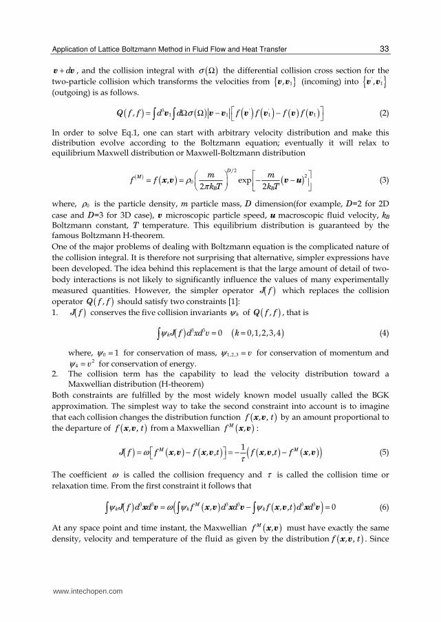
4.6 Thermal boundary treatment Considering the thermal boundary conditions, the fluid flow boundary treatments (such as bounce back boundary, extrapolation boundary) can also be used by the temperature variable. However, it has been confirmed that [25-27], to date, the model of assuming a counter slip thermal energy density boundary is of the highest accurate boundary treatments because it can guarantee the fixed velocity and temperature or heat flux at the wall exactly. For the isothemal wall boundary case, the temperature is fixed as T0 at the solid surface pointing to the fluid region. After streaming, g2, g5 and g6 are unknows, as shown in Figure 10.
2 5
4 8
6
7
Fluid
Solid
1 3 0
Fig. 10. Counter slip thermal boundary for D2Q9 lattice
Assume these unknown temperature density distributions are equal to their temperature
density equilibrium distributions with unknown temperature T* . Adding these three
unknown temperature density distributions together (e.g., for the passive scalar thermal
LBE model), it yields:
( )y yg g g T u u* 22 5 6
11 3 3
6+ + = + + (84)
where yu is the velocity normal to the wall and the x velocity (ux) is assumed to be zero. If
the value of T* is known, the unknown temperature density distributions (g2, g5 and g6) can
be solved by using the corresponding temperature equilibrium distribution functions.
Meanwhile, note that for the isothermal wall, it reads:
g T0α
α
= (85)
www.intechopen.com

Application of Lattice Boltzmann Method in Fluid Flow and Heat Transfer
53
Substitute Eq.84 into Eq.85 and solve for T* , it shows:
( )y y
T T g g g g g gu u
*0 0 1 3 4 7 82
6
1 3 3= − − − − − −
+ + (86)
Eventually, the three unknown temperature density distributions (g2, g5 and g6) can be
obtained by substituting T* into the temperature density equilibrium distributions.
Obviously, this method can be easily extended to the 3D case without any difficulties. For the heat flux boundary condition, a second order finite difference scheme is used to evaluate the temperature on the wall,
i i i
y
T T T Tq
y y
,1 ,2 ,3
0
3 4
2=
∂ − + −= =
∂ Δ (87)
After finding the wall temperature, the same procedure as described in the isothermal wall case is used to calculate the unknown temperature density distributions.
4.7 Body force treatment Since there exist all kinds of body forces (e.g., gravity, centrifugal force) in the real case simulations, how to deal with the body force in the LBE model is another important issue needed to be done before this method can be widely used in the real applications. Consider the Newton’s second law of motion, we have
d
m mdt
= =u
F a (88)
Recognizing that the density is proportional to the mass, the lattice length is the unit length in the LBE model (which means the volume for each basic lattice is also unit) and that the relaxation time τ is the elementary time of collisions, then rearrange Eq.88, it yields:
τ
ρ
⋅Δ =
Fu (89)
where Δu is a increment in velocity due to the external body force. Finally, it can be written
down like:
eq( ) τ
ρ
⋅= + Δ = +
Fu u u u (90)
where eq( )u is used to compute the equilibrium distribution functions, eqf ( ) , and u comes
from the summation over the local distribution functions, fα , like Eq.17.
5. Application of Lattice Boltzmann model
In the previous sections, the LBE fluid flow, heat transfer models and the corresponding boundary treatments have been discussed in details. In this section, these models will be used to solve the fully developed fluid flow and heat transfer problem in a curved square duct to validate this new approach. The D3Q27 incompressible fluid flow and passive scalar
www.intechopen.com

Computational Fluid Dynamics Technologies and Applications
54
thermal LBE models are adopted to simulate the fully developed fluid flow and heat transfer in the curved square duct, and the flow driven force, i.e., pressure difference, and centrifugal force, will be taken into account in the models like body force acting on each lattice.
5.1 Fluid flow and heat transfer in curved square duct The study of viscous flow in the curved ducts is of fundamental interest in fluid mechanics because of the numerous applications such as flows through turbo machinery blade passages, aircraft intakes, diffusers, heat exchangers etc. [28]. The major effect of curved duct on the fluid flow involves the strong secondary flow due to the longitudinal curvature in the geometry. The presence of longitudinal curvature generates the centrifugal force perpendicular to the main flow along the axis and produces the so-called secondary flow on the cross section of ducts. As a consequence of this centrifugal force, the axial velocity profile will be distorted (from the typical-parabolic velocity profile in straight ducts) with an outward shift of the peak axial velocity, and at the same time, the total flow rate will be reduced due to the decrease of average axial velocity.
L
a
a
b bRo
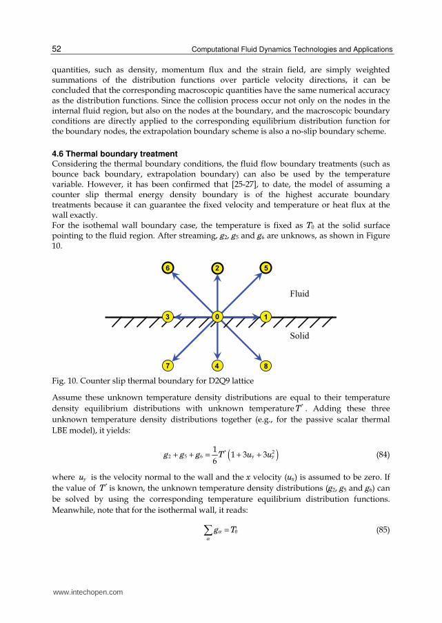
Fig. 11. The geometry configuration of curved square duct
As shown in Figure 11, a curved square duct with side length L is placed on the horizontal plane and the radius of the curved duct is R, measured from the center of duct to the center of the curve. The fluid flows in the square duct about the center of curvature toward the inside of the plane of the paper. The curvature ratio of this curved duct is defined as:
hD
CR
= (91)
Where, Dh is the equivalent hydrodynamic diameter of square duct, which is defined as
h
A LD L
P L
24 4
4= = = (92)
www.intechopen.com
Application of Lattice Boltzmann Method in Fluid Flow and Heat Transfer
55
The non-dimensional characteristic Dean number is defined as the function of Reynolds number and curvature ratio.
( )n eD R C0.5
= ⋅ (93)
h
e
U DR
υ
⋅= (94)
where, Re is the Reynolds number of the duct flow. A uniform grid is used in this article, and the corresponding relaxation factors for fluid flow and heat transfer are in the range of 0.6 ~1.0. On each cross section of curved duct, a constant pressure gradient is introduced to drive fluid flow along the duct’s axial direction. Due to the longitudinal curvature and axial velocity, the centrifugal force is involved and drives the fluid flow far away from the center of curved duct (i.e., point O as shown in Figure 11), and then the so-called secondary flow is formed on the cross section. In this article, both pressure gradient and centrifugal force are treated like body forces acting on each interior lattice with different directions on the cross section of duct (which is the projection of the computational domain), and the macroscopic momentum conservation method [23, 24] is used to apply these body forces to the LBE fluid flow and heat transfer models. As shown in Figure 11, the fluid flows in the square duct pointing toward the inside of the plane of the paper. Since the fully developed fluid flow and heat transfer will be studied numerically in this section, the axial velocity profile and dimensionless temperature distribution on the cross section will not be changed along the main flow direction. Therefore, the original computation domain, which consists of the square cross section and curved duct, can be simplified to a domain including the square cross section and a few lattice lengths perpendicular to this section plane. As a result of this simplification, the basic LBM with uniform lattice can be used to solve this problem without any special treatment for the curved boundary. It is worth noting that although the original computation domain has been simplified, the fluid flow and heat transfer simulations are still in three dimensions, i.e., two dimensions on the cross section and one dimension in the axial flow direction. For fluid flow in pipes, the Fanning friction factor is defined as [25]:
w
f
avg
CV 2
.
2 τ
ρ
⋅=
⋅ (95)
where wτ is the average wall shear stress and is defined as:
z
w
dU
dnτ µ= ⋅ (96)
Plugging Eq.96 and Eq.94 into Eq.95 and rearranging, one obtains the following friction factor for the curved duct.
h z
f e
avg
D dUC R
V dn.
2 ⋅⋅ = ⋅ (97)
www.intechopen.com

Computational Fluid Dynamics Technologies and Applications
56
As far as fluid flow in straight square duct is concerned, the analytical friction factor is available in literature and equals 14.25 [26]. For heat transfer in curved duct, the corresponding dimensionless temperature and Nusselt number are defined as follows:
w
w m
T TT
T T
* −=
− (98)
h
u
h DN
k
⋅= (99)
where Tw and Tm are the wall temperature and mean temperature across the duct, receptively.
h is the average heat transfer coefficient around the four wall sides and is defined as:
w m
Tk
nhT T
∂− ⋅
∂=−
(100)
Plugging Eq.98 and Eq.100 into Eq.99 and rearranging, one obtains:
u h
TN D
n
*∂= ⋅
∂ (101)
For the fluid flow and heat transfer in a straight square duct, the analytical Nusselt number with constant wall temperature is 2.98 [26]. In order to obtain more accurate results, the two-dimensional Simpson integration method is used to calculate the average axial velocity based on the uniform lattice on the cross section.
5.2 Boundary conditions In the simplified computation domain, the boundary conditions have to be specified in two parts with three directions, i.e., axial flow direction and two directions on the cross section plane. Axial flow direction: Since both the fluid flow and heat transfer are fully developed, the velocity and dimensionless temperature profiles will not change along the axial flow direction (which is perpendicular to the plane of the paper and toward inside). Therefore, the simple periodic boundary can be naturally applied for both fluid flow and heat transfer in this direction, without any special treatment for the curved boundary. Cross section plane: On the duct cross section, four sides of wall are needed to specify the boundary conditions. In this mathematic model, the no-slip boundary and constant wall temperature conditions are applied on the four duct walls for fluid flow and heat transfer, respectively. The second-order extrapolation boundary treatment [27] and counter-slip thermal boundary treatment [28] are employed for the fluid flow and heat transfer to determine the unknown distributions (i.e., pressure and dimensionless temperature distributions) coming from outside the computation domain. Once all these boundary conditions are established, the fully developed fluid flow and heat transfer in the straight square duct are simulated using the current LBM model by letting curvature ratio approach to zero (i.e., the radius of curved duct, R, is big enough, for example, 109), and the converging criterion in this test simulation is that the relative error of
www.intechopen.com

Application of Lattice Boltzmann Method in Fluid Flow and Heat Transfer
57
total velocity (including three components) on each uniform lattice is less than 1.0×10⁻⁴ for every 400 consecutive time steps. After the converging criterion is reached, the simulation results show that both friction coefficient and Nusselt number are very in good agreement with analytical results (i.e., the relative errors versus analytical results are less than 0.1%). This validates that this LBM model is correct and the simplification of computation domain is feasible and applicable. In addition to this bench mark validation of the straight duct, a grid convergence test was implemented before any data were adopted. For a given fluid flow problem, different number of uniform lattices (i.e., 50×50×3,100×100×3 and 160×160×3, where three lattices are used for the periodic direction) for the same computation domain were used to compare the differences in terms of friction coefficient and flow pattern on the cross section. After a couple of comparisons, it was found that the uniform lattice 100×100×3 has both good accuracy and less computing cost. Therefore, 100×100×3 uniform lattice mesh is used in this article to simulate the fluid flow and heat transfer problems.
5.3 Simulation results and discussion 5.3.1 Fluid flow As shown in Figure 12, the non-dimensional axial velocity distribution of cross section b-b is presented at different Dean number with a constant curvature ratio, C =0.05. From this Figure, it is evident that, as the Dean number increases, the maximum axial velocity first shifts toward the outside of the duct from near the center position until it reaches a most outside point on the cross section; and then once the Dean number reaches a certain value (which is a function of the curvature ratio), the velocity profile on cross section b-b suddenly changes to a new pattern (as shown in Figure 12), and the location of maximum axial velocity is much closer to the center of duct than before. Moreover, as Dean number increases further, the maximum axial velocity moves toward the center of duct, which is the opposite moving direction compared to the case with smaller Dean number before the new velocity profile was observed.
X/L
U/U
ave
.
0 0.2 0.4 0.6 0.8 10
0.5
1
1.5
2
2.5
Dn=20.0
Dn=50.0
Dn=100.0
Dn=150.0
Dn=200.0
Dn=300.0
Curvature ratio: 0.05
Fig. 12. Velocity distributions along b-b cross section
With the same conditions, the dimensionless axial velocity profile along cross section a-a is shown in Figure 13. In this Figure, it is apparent that as the Dean number increases, the peak of velocity profile on cross section a-a changes from one point at the beginning to two symmetrical points, and eventually up to three points (one is at the center and the other two
www.intechopen.com

Computational Fluid Dynamics Technologies and Applications
58
are symmetrical about the center one). Meanwhile, the axial velocity on this cross section a-a is becoming more uniform as Dean number increases. The switchback movement of maximum axial velocity on cross section b-b in Figure 12 and the change of number of peak velocities on plane a-a in Figure 13 can be explained as follows. On the duct cross section, the centrifugal force (which is induced by axial velocity and duct curvature) drives the fluid flow from inner side wall to the outer side wall and this fluid flow causes a symmetrical flow pattern on the cross section for the horizontal curved duct. Compared to the main axial fluid flow (which is perpendicular to cross section), the flow on the cross section is called secondary flow. When the Dean number is small, there is just one peak point on the axial velocity profile, and the secondary flow is one pair of weak symmetrical eddies due to the small centrifugal force. As Dean number keeps increasing, the axial maximum velocity moves toward the outside of wall and, at the same time, the two symmetrical eddies become stronger and stronger, eventually distorting the axial velocity from a single peak to two symmetrical peaks on cross section a-a. On the other hand, once Dean number exceeds a certain value, the secondary flow suddenly changes from one pair symmetrical eddies to two pairs of symmetrical eddies (having opposite rotating directions) due to the imbalance between centrifugal force and pressure gradient on the cross section. This is the so-called Dean instability [29, 30]. Therefore, the velocity distribution on section b-b suddenly changes and another peak velocity appears at cross section a-a, that is, there are now three peak velocities.
Y/L
U/U
ave
.
0 0.2 0.4 0.6 0.8 10
0.5
1
1.5
2
2.5
Dn=20.0
Dn=50.0
Dn=100.0
Dn=150.0
Dn=200.0
Dn=300.0
Curvature ratio: 0.05
Fig. 13. Velocity distributions along a-a cross section
In Figures 14 to 17 or 18 to 21, the detailed dimensionless axial velocity distributions are presented and the transition process from one velocity peak to two peaks and eventually to three peaks are all clearly shown (i.e., Figures 14- 16 or 18- 20 in 3-D view). Based on these axial velocity contours, it is obvious that the higher Dean number, the greater velocity gradient that will be observed around the duct walls, especially for the two vertical sides, and this is consistent with the previous results in Figure 13. Moreover, since the axial velocity with the same number of uniform contour lines is provided at different Dean numbers, the distribution of uniform contour lines shows how well the axial velocity distribute uniformly on the cross section. From Figures 15-17 or 19-21, one can conclude that the axial velocity trends to be more uniform on the cross section area as Dean number increases, which is also consistent with Figures 22 and 23.
www.intechopen.com

Application of Lattice Boltzmann Method in Fluid Flow and Heat Transfer
59
Inner side Outer side Inner side Outer side
Fig. 14. Velocity contour of cross section (Dn=50.0 C=0.05)
Fig. 15. Velocity contour of cross section (Dn=100.0 C=0.05)
Inner side Outer side Inner side Outer side Fig. 16. Velocity contour of cross section (Dn=150.0 C=0.05)
Fig. 17. Velocity contour of cross section (Dn=200.0 C=0.05)
0.00
0.50
1.00
1.50
2.00
U/U
ave
.
0.00
0.50
1.00
1.50
2.00
XY
Z 0.00
0.50
1.00
1.50
2.00
U/U
ave
.
0.00
0.50
1.00
1.50
2.00
XY
Z
Fig. 18. Axial velocity profile in 3D view (Dn=50.0 C=0.05)
Fig. 19. Axial velocity profile in 3D view (Dn=100.0 C=0.05)
www.intechopen.com

Computational Fluid Dynamics Technologies and Applications
60
0.00
0.50
1.00
1.50
2.00
U/U
ave
.0.00
0.50
1.00
1.50
2.00
XY
Z0.00
0.50
1.00
1.50
2.00
U/U
ave
.
0.00
0.50
1.00
1.50
2.00
XY
Z
Fig. 20. Axial velocity profile in 3D view (Dn=150.0 C=0.05)
Fig. 21. Axial velocity profile in 3D view (Dn=200.0 C=0.05)
Inner side Outer side Inner side Outer side Fig. 22. Velocity vector of cross section (Dn=50.0 C=0.05)
Fig. 23. Velocity vector of cross section (Dn=100.0 C=0.05)
Inner side Outer side Inner side Outer side
Fig. 24. Velocity vector of cross section (Dn=150.0 C=0.05)
Fig. 25. Velocity vector of cross section (Dn=200.0 C=0.05)
www.intechopen.com
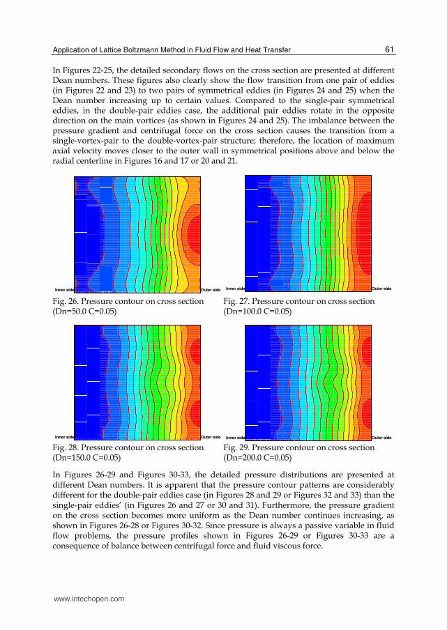
Application of Lattice Boltzmann Method in Fluid Flow and Heat Transfer
61
In Figures 22-25, the detailed secondary flows on the cross section are presented at different Dean numbers. These figures also clearly show the flow transition from one pair of eddies (in Figures 22 and 23) to two pairs of symmetrical eddies (in Figures 24 and 25) when the Dean number increasing up to certain values. Compared to the single-pair symmetrical eddies, in the double-pair eddies case, the additional pair eddies rotate in the opposite direction on the main vortices (as shown in Figures 24 and 25). The imbalance between the pressure gradient and centrifugal force on the cross section causes the transition from a single-vortex-pair to the double-vortex-pair structure; therefore, the location of maximum axial velocity moves closer to the outer wall in symmetrical positions above and below the radial centerline in Figures 16 and 17 or 20 and 21.
Inner side Outer side Inner side Outer side
Fig. 26. Pressure contour on cross section (Dn=50.0 C=0.05)
Fig. 27. Pressure contour on cross section (Dn=100.0 C=0.05)
Inner side Outer side Inner side Outer side Fig. 28. Pressure contour on cross section (Dn=150.0 C=0.05)
Fig. 29. Pressure contour on cross section (Dn=200.0 C=0.05)
In Figures 26-29 and Figures 30-33, the detailed pressure distributions are presented at different Dean numbers. It is apparent that the pressure contour patterns are considerably different for the double-pair eddies case (in Figures 28 and 29 or Figures 32 and 33) than the single-pair eddies’ (in Figures 26 and 27 or 30 and 31). Furthermore, the pressure gradient on the cross section becomes more uniform as the Dean number continues increasing, as shown in Figures 26-28 or Figures 30-32. Since pressure is always a passive variable in fluid flow problems, the pressure profiles shown in Figures 26-29 or Figures 30-33 are a consequence of balance between centrifugal force and fluid viscous force.
www.intechopen.com

Computational Fluid Dynamics Technologies and Applications
62
-4500.0
-2500.0
-500.0
1500.0
3500.0
5500.0
7500.0
P-P
0(P
a)
-4500.0
-2500.0
-500.0
1500.0
3500.0
5500.0
7500.0
XY
Z -14000.0
-8000.0
-2000.0
4000.0
10000.0
16000.0
22000.0
P-P
0(P
a)
-14000.0
-8000.0
-2000.0
4000.0
10000.0
16000.0
22000.0
XY
Z
Fig. 30. Pressure profile in 3D view (Dn=50.0 C=0.05)
Fig. 31. Pressure profile in 3D view (Dn=100.0 C=0.05)
-30000.0
-16000.0
-2000.0
12000.0
26000.0
40000.0
54000.0
P-P
0(P
a)
-30000.0
-16000.0
-2000.0
12000.0
26000.0
40000.0
54000.0
XY
Z
-50000.0
-25000.0
0.0
25000.0
50000.0
75000.0
100000.0
P-P
0(P
a)
-50000.0
-25000.0
0.0
25000.0
50000.0
75000.0
100000.0
XY
Z
Fig. 32. Pressure profile in 3D view (Dn=150.0 C=0.05)
Fig. 33. Pressure profile in 3D view (Dn=200.0 C=0.05)
In real engineering applications, one of the most important results of fully developed flow in curved square duct is estimation of the friction factor (or flow-rate reduction). The available well-known friction factor correlation in the literature [31] is:
c sf f Dn 0.39/ 0.225= for square duct with 100<Dn<1500 (102)
In Figure 34, the computed friction factor ratios for a straight square duct at different curvature ratio are presented. It is evident that the presented LBM simulation results are in good agreement with the experimental correlation. On the other hand, it is clearly shown in this Figure that the friction coefficient for each specific curvature ratio (from 0.05 to 1.00) changes suddenly when the Dean number is between 115 and 130. This is because when Dean number increases from 115 to 130, the flow pattern on cross section changes from one pair of eddies to two pairs of eddies. This Dean number which identifies the flow pattern is called critical Dean number. As a consequence of flow pattern change, the corresponding friction coefficient is increased.
www.intechopen.com
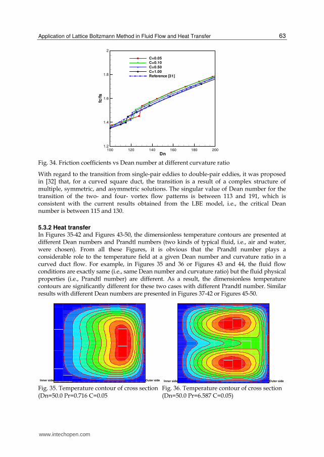
Application of Lattice Boltzmann Method in Fluid Flow and Heat Transfer
63
Dn
fc/f
s
100 120 140 160 180 2001.2
1.4
1.6
1.8
2
C=0.05C=0.10
C=0.50
C=1.00Reference [31]
Fig. 34. Friction coefficients vs Dean number at different curvature ratio
With regard to the transition from single-pair eddies to double-pair eddies, it was proposed in [32] that, for a curved square duct, the transition is a result of a complex structure of multiple, symmetric, and asymmetric solutions. The singular value of Dean number for the transition of the two- and four- vortex flow patterns is between 113 and 191, which is consistent with the current results obtained from the LBE model, i.e., the critical Dean number is between 115 and 130.
5.3.2 Heat transfer In Figures 35-42 and Figures 43-50, the dimensionless temperature contours are presented at different Dean numbers and Prandtl numbers (two kinds of typical fluid, i.e., air and water, were chosen). From all these Figures, it is obvious that the Prandtl number plays a considerable role to the temperature field at a given Dean number and curvature ratio in a curved duct flow. For example, in Figures 35 and 36 or Figures 43 and 44, the fluid flow conditions are exactly same (i.e., same Dean number and curvature ratio) but the fluid physical properties (i.e., Prandtl number) are different. As a result, the dimensionless temperature contours are significantly different for these two cases with different Prandtl number. Similar results with different Dean numbers are presented in Figures 37-42 or Figures 45-50.
Inner side Outer side Inner side Outer side Fig. 35. Temperature contour of cross section (Dn=50.0 Pr=0.716 C=0.05
Fig. 36. Temperature contour of cross section (Dn=50.0 Pr=6.587 C=0.05)
www.intechopen.com
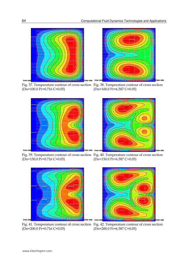
Computational Fluid Dynamics Technologies and Applications
64
Inner side Outer side Inner side Outer side Fig. 37. Temperature contour of cross section (Dn=100.0 Pr=0.716 C=0.05)
Fig. 38. Temperature contour of cross section (Dn=100.0 Pr=6.587 C=0.05)
Inner side Outer side Inner side Outer side Fig. 39. Temperature contour of cross section (Dn=150.0 Pr=0.716 C=0.05)
Fig. 40. Temperature contour of cross section (Dn=150.0 Pr=6.587 C=0.05)
Inner side Outer side Inner side Outer side Fig. 41. Temperature contour of cross section (Dn=200.0 Pr=0.716 C=0.05)
Fig. 42. Temperature contour of cross section (Dn=200.0 Pr=6.587 C=0.05)
www.intechopen.com
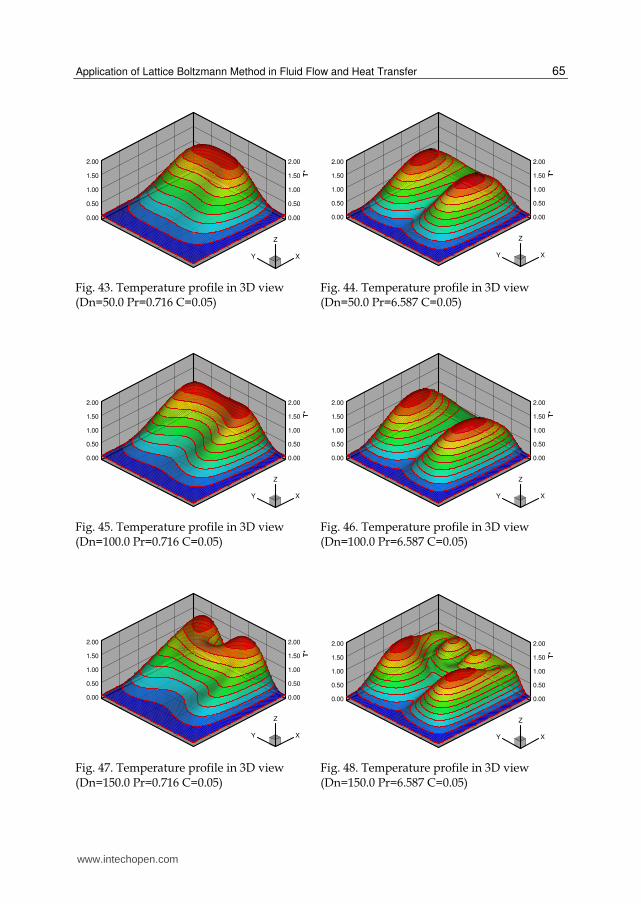
Application of Lattice Boltzmann Method in Fluid Flow and Heat Transfer
65
0.00
0.50
1.00
1.50
2.00
T*
0.00
0.50
1.00
1.50
2.00
XY
Z
0.00
0.50
1.00
1.50
2.00
T*
0.00
0.50
1.00
1.50
2.00
XY
Z
Fig. 43. Temperature profile in 3D view (Dn=50.0 Pr=0.716 C=0.05)
Fig. 44. Temperature profile in 3D view (Dn=50.0 Pr=6.587 C=0.05)
0.00
0.50
1.00
1.50
2.00
T*
0.00
0.50
1.00
1.50
2.00
XY
Z
0.00
0.50
1.00
1.50
2.00
T*
0.00
0.50
1.00
1.50
2.00
XY
Z
Fig. 45. Temperature profile in 3D view (Dn=100.0 Pr=0.716 C=0.05)
Fig. 46. Temperature profile in 3D view (Dn=100.0 Pr=6.587 C=0.05)
0.00
0.50
1.00
1.50
2.00
T*
0.00
0.50
1.00
1.50
2.00
XY
Z
0.00
0.50
1.00
1.50
2.00
T*
0.00
0.50
1.00
1.50
2.00
XY
Z
Fig. 47. Temperature profile in 3D view (Dn=150.0 Pr=0.716 C=0.05)
Fig. 48. Temperature profile in 3D view (Dn=150.0 Pr=6.587 C=0.05)
www.intechopen.com
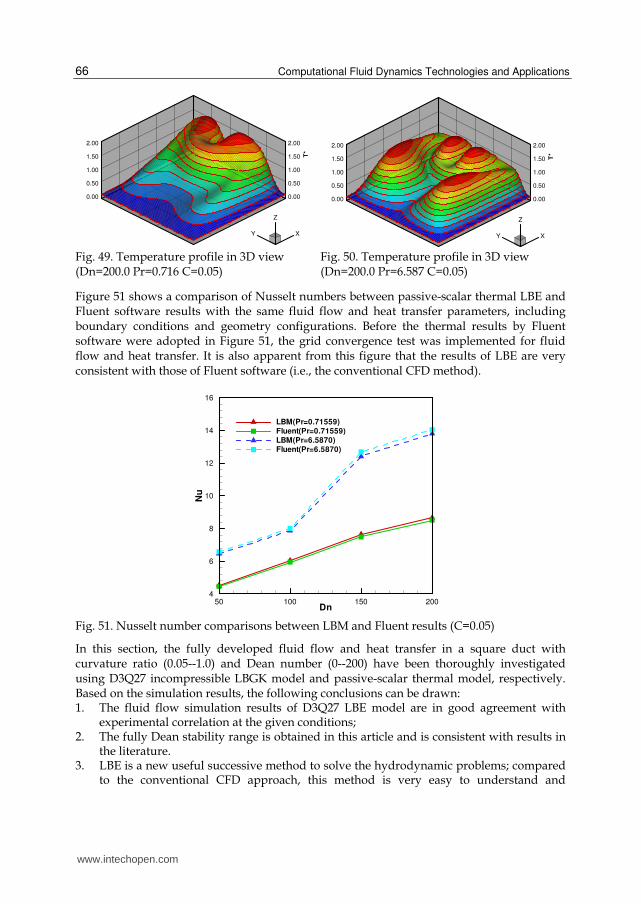
Computational Fluid Dynamics Technologies and Applications
66
0.00
0.50
1.00
1.50
2.00
T*
0.00
0.50
1.00
1.50
2.00
XY
Z
0.00
0.50
1.00
1.50
2.00
T*
0.00
0.50
1.00
1.50
2.00
XY
Z
Fig. 49. Temperature profile in 3D view (Dn=200.0 Pr=0.716 C=0.05)
Fig. 50. Temperature profile in 3D view (Dn=200.0 Pr=6.587 C=0.05)
Figure 51 shows a comparison of Nusselt numbers between passive-scalar thermal LBE and Fluent software results with the same fluid flow and heat transfer parameters, including boundary conditions and geometry configurations. Before the thermal results by Fluent software were adopted in Figure 51, the grid convergence test was implemented for fluid flow and heat transfer. It is also apparent from this figure that the results of LBE are very consistent with those of Fluent software (i.e., the conventional CFD method).
Dn
Nu
50 100 150 2004
6
8
10
12
14
16
LBM(Pr=0.71559)Fluent(Pr=0.71559)LBM(Pr=6.5870)Fluent(Pr=6.5870)
Fig. 51. Nusselt number comparisons between LBM and Fluent results (C=0.05)
In this section, the fully developed fluid flow and heat transfer in a square duct with curvature ratio (0.05--1.0) and Dean number (0--200) have been thoroughly investigated using D3Q27 incompressible LBGK model and passive-scalar thermal model, respectively. Based on the simulation results, the following conclusions can be drawn: 1. The fluid flow simulation results of D3Q27 LBE model are in good agreement with
experimental correlation at the given conditions; 2. The fully Dean stability range is obtained in this article and is consistent with results in
the literature. 3. LBE is a new useful successive method to solve the hydrodynamic problems; compared
to the conventional CFD approach, this method is very easy to understand and
www.intechopen.com
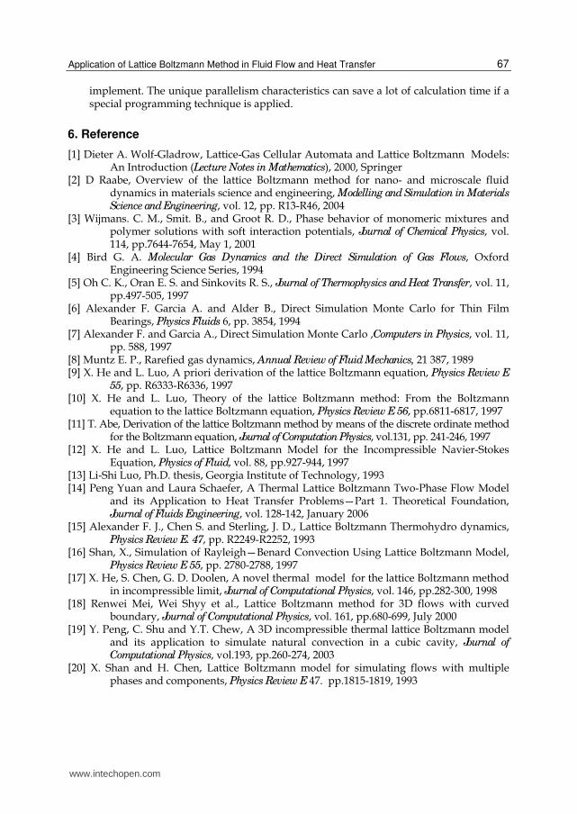
Application of Lattice Boltzmann Method in Fluid Flow and Heat Transfer
67
implement. The unique parallelism characteristics can save a lot of calculation time if a special programming technique is applied.
6. Reference
[1] Dieter A. Wolf-Gladrow, Lattice-Gas Cellular Automata and Lattice Boltzmann Models: An Introduction (Lecture Notes in Mathematics), 2000, Springer
[2] D Raabe, Overview of the lattice Boltzmann method for nano- and microscale fluid dynamics in materials science and engineering, Modelling and Simulation in Materials
Science and Engineering, vol. 12, pp. R13-R46, 2004 [3] Wijmans. C. M., Smit. B., and Groot R. D., Phase behavior of monomeric mixtures and
polymer solutions with soft interaction potentials, Journal of Chemical Physics, vol. 114, pp.7644-7654, May 1, 2001
[4] Bird G. A. Molecular Gas Dynamics and the Direct Simulation of Gas Flows, Oxford Engineering Science Series, 1994
[5] Oh C. K., Oran E. S. and Sinkovits R. S., Journal of Thermophysics and Heat Transfer, vol. 11, pp.497-505, 1997
[6] Alexander F. Garcia A. and Alder B., Direct Simulation Monte Carlo for Thin Film Bearings, Physics Fluids 6, pp. 3854, 1994
[7] Alexander F. and Garcia A., Direct Simulation Monte Carlo ,Computers in Physics, vol. 11, pp. 588, 1997
[8] Muntz E. P., Rarefied gas dynamics, Annual Review of Fluid Mechanics, 21 387, 1989 [9] X. He and L. Luo, A priori derivation of the lattice Boltzmann equation, Physics Review E
55, pp. R6333-R6336, 1997 [10] X. He and L. Luo, Theory of the lattice Boltzmann method: From the Boltzmann
equation to the lattice Boltzmann equation, Physics Review E 56, pp.6811-6817, 1997 [11] T. Abe, Derivation of the lattice Boltzmann method by means of the discrete ordinate method
for the Boltzmann equation, Journal of Computation Physics, vol.131, pp. 241-246, 1997 [12] X. He and L. Luo, Lattice Boltzmann Model for the Incompressible Navier-Stokes
Equation, Physics of Fluid, vol. 88, pp.927-944, 1997 [13] Li-Shi Luo, Ph.D. thesis, Georgia Institute of Technology, 1993 [14] Peng Yuan and Laura Schaefer, A Thermal Lattice Boltzmann Two-Phase Flow Model
and its Application to Heat Transfer Problems—Part 1. Theoretical Foundation, Journal of Fluids Engineering, vol. 128-142, January 2006
[15] Alexander F. J., Chen S. and Sterling, J. D., Lattice Boltzmann Thermohydro dynamics, Physics Review E. 47, pp. R2249-R2252, 1993
[16] Shan, X., Simulation of Rayleigh—Benard Convection Using Lattice Boltzmann Model, Physics Review E 55, pp. 2780-2788, 1997
[17] X. He, S. Chen, G. D. Doolen, A novel thermal model for the lattice Boltzmann method in incompressible limit, Journal of Computational Physics, vol. 146, pp.282-300, 1998
[18] Renwei Mei, Wei Shyy et al., Lattice Boltzmann method for 3D flows with curved boundary, Journal of Computational Physics, vol. 161, pp.680-699, July 2000
[19] Y. Peng, C. Shu and Y.T. Chew, A 3D incompressible thermal lattice Boltzmann model and its application to simulate natural convection in a cubic cavity, Journal of
Computational Physics, vol.193, pp.260-274, 2003 [20] X. Shan and H. Chen, Lattice Boltzmann model for simulating flows with multiple
phases and components, Physics Review E 47. pp.1815-1819, 1993
www.intechopen.com
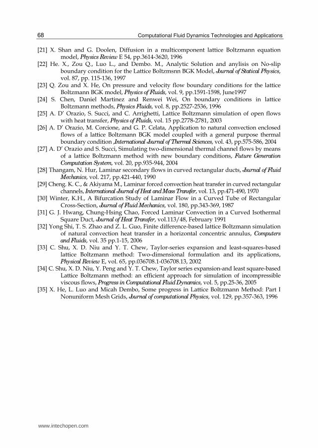
Computational Fluid Dynamics Technologies and Applications
68
[21] X. Shan and G. Doolen, Diffusion in a multicomponent lattice Boltzmann equation model, Physics Review E 54, pp.3614-3620, 1996
[22] He. X., Zou Q., Luo L., and Dembo. M., Analytic Solution and anylisis on No-slip boundary condition for the Lattice Boltzmsnn BGK Model, Journal of Statical Physics, vol. 87, pp. 115-136, 1997
[23] Q. Zou and X. He, On pressure and velocity flow boundary conditions for the lattice Boltzmann BGK model, Physics of Fluids, vol. 9, pp.1591-1598, June1997
[24] S. Chen, Daniel Martinez and Renwei Wei, On boundary conditions in lattice Boltzmann methods, Physics Fluids, vol. 8, pp.2527-2536, 1996
[25] A. D’ Orazio, S. Succi, and C. Arrighetti, Lattice Boltzmann simulation of open flows with heat transfer, Physics of Fluids, vol. 15 pp.2778-2781, 2003
[26] A. D’ Orazio, M. Corcione, and G. P. Celata, Application to natural convection enclosed flows of a lattice Boltzmann BGK model coupled with a general purpose thermal boundary condition ,International Journal of Thermal Sciences, vol. 43, pp.575-586, 2004
[27] A. D’ Orazio and S. Succi, Simulating two-dimensional thermal channel flows by means of a lattice Boltzmann method with new boundary conditions, Future Generation
Computation System, vol. 20, pp.935-944, 2004 [28] Thangam, N. Hur, Laminar secondary flows in curved rectangular ducts, Journal of Fluid
Mechanics, vol. 217, pp.421-440, 1990 [29] Cheng. K. C., & Akiyama M., Laminar forced convection heat transfer in curved rectangular
channels, International Journal of Heat and Mass Transfer, vol. 13, pp.471-490, 1970 [30] Winter, K.H., A Bifurcation Study of Laminar Flow in a Curved Tube of Rectangular
Cross-Section, Journal of Fluid Mechanics, vol. 180, pp.343-369, 1987 [31] G. J. Hwang, Chung-Hsing Chao, Forced Laminar Convection in a Curved Isothermal
Square Duct, Journal of Heat Transfer, vol.113/48, February 1991 [32] Yong Shi, T. S. Zhao and Z. L. Guo, Finite difference-based lattice Boltzmann simulation
of natural convection heat transfer in a horizontal concentric annulus, Computers and Fluids, vol. 35 pp.1-15, 2006
[33] C. Shu, X. D. Niu and Y. T. Chew, Taylor-series expansion and least-squares-based lattice Boltzmann method: Two-dimensional formulation and its applications, Physical Review E, vol. 65, pp.036708.1-036708.13, 2002
[34] C. Shu, X. D. Niu, Y. Peng and Y. T. Chew, Taylor series expansion-and least square-based Lattice Boltzmann method: an efficient approach for simulation of incompressible viscous flows, Progress in Computational Fluid Dynamics, vol. 5, pp.25-36, 2005
[35] X. He, L. Luo and Micah Dembo, Some progress in Lattice Boltzmann Method: Part I Nonuniform Mesh Grids, Journal of computational Physics, vol. 129, pp.357-363, 1996
www.intechopen.com

Computational Fluid Dynamics Technologies and ApplicationsEdited by Prof. Igor Minin
ISBN 978-953-307-169-5Hard cover, 396 pagesPublisher InTechPublished online 05, July, 2011Published in print edition July, 2011
InTech EuropeUniversity Campus STeP Ri Slavka Krautzeka 83/A 51000 Rijeka, Croatia Phone: +385 (51) 770 447 Fax: +385 (51) 686 166www.intechopen.com
InTech ChinaUnit 405, Office Block, Hotel Equatorial Shanghai No.65, Yan An Road (West), Shanghai, 200040, China
Phone: +86-21-62489820 Fax: +86-21-62489821
This book is planned to publish with an objective to provide a state-of-art reference book in the area ofcomputational fluid dynamics for CFD engineers, scientists, applied physicists and post-graduate students.Also the aim of the book is the continuous and timely dissemination of new and innovative CFD research anddevelopments. This reference book is a collection of 14 chapters characterized in 4 parts: modern principles ofCFD, CFD in physics, industrial and in castle. This book provides a comprehensive overview of thecomputational experiment technology, numerical simulation of the hydrodynamics and heat transfer processesin a two dimensional gas, application of lattice Boltzmann method in heat transfer and fluid flow, etc. Severalinteresting applications area are also discusses in the book like underwater vehicle propeller, the flow behaviorin gas-cooled nuclear reactors, simulation odour dispersion around windbreaks and so on.
How to referenceIn order to correctly reference this scholarly work, feel free to copy and paste the following:
Quan Liao and Tien-Chien Jen (2011). Application of Lattice Boltzmann Method in Fluid Flow and HeatTransfer, Computational Fluid Dynamics Technologies and Applications, Prof. Igor Minin (Ed.), ISBN: 978-953-307-169-5, InTech, Available from: http://www.intechopen.com/books/computational-fluid-dynamics-technologies-and-applications/application-of-lattice-boltzmann-method-in-fluid-flow-and-heat-transfer

© 2011 The Author(s). Licensee IntechOpen. This chapter is distributedunder the terms of the Creative Commons Attribution-NonCommercial-ShareAlike-3.0 License, which permits use, distribution and reproduction fornon-commercial purposes, provided the original is properly cited andderivative works building on this content are distributed under the samelicense.