application of earth observation and related …

APPLICATION OF EARTH OBSERVATION AND RELATED TECHNOLOGY IN AGRO-

HYDROLOGICAL MODELING

By

Matthew Ryan Herman

A DISSERTATION

Submitted to

Michigan State University

in partial fulfillment of the requirements

for the degree of

Biosystems Engineering – Doctor of Philosophy

2018

ABSTRACT

APPLICATION OF EARTH OBSERVATION AND RELATED TECHNOLOGY IN AGRO-

HYDROLOGICAL MODELING

By

Matthew Ryan Herman

Freshwater is vital for life on Earth, and as the human population continues to grow so

does the demand for this limited resource. However, anthropogenic activities and climate change

will continue to alter freshwater systems. Therefore, there is a need to understand how the

hydrological cycle is changing across the landscape. Traditionally, this has been done by single

point monitoring stations; however, these stations do not have the spatial variability to capture

different aspects of the hydrologic cycle required for detailed analysis. Therefore, hydrological

models are traditionally calibrated and validated against a single or a few monitoring stations.

One solution to this issue is the incorporation of remote sensing data. However, the proper use of

these products has not been well documented in hydrological models. Furthermore, with a wide

variety of different remote sensing datasets, it is challenging to know which datasets/products

should be used when.

To address these knowledge gaps, three studies were conducted. The first study was

performed to examine whether the incorporation of remotely sensed and spatially distributed

datasets can improve the overall model performance. In this study, the applicability of two

remote sensing actual evapotranspiration (ETa) products (the Simplified Surface Energy Balance

(SSEBop) and the Atmosphere-Land Exchange Inverse (ALEXI)) were examined to improve the

performance of a hydrologic model using two different calibration techniques (genetic algorithm

and multi-variable). Results from this study showed that the inclusion of ETa remote sensing

data along with the multi-variable calibration technique could improve the overall performance

of a hydrological model.

The second study evaluated the spatial and temporal performance of eight ETa remote

sensing products in a region that lacks observed data. The remotely sensed datasets were further

compared with ETa results from a physically-based hydrologic model to examine the differences

and describe discrepancy among them. All of these datasets were compared through the use of

the Generalized Least-Square estimation with Autoregressive models that compared the ETa

datasets on temporal (i.e., monthly and seasonal basis) and spatial (i.e., landuse) scales at both

watershed and subbasin levels. Results showed a lack of patterns among the datasets when

evaluating the monthly ETa variations; however, the seasonal aggregated data presented a better

pattern and fewer variances, and statistical difference at the 0.05 level during spring and summer

compared to fall and winter months. Meanwhile, spatial analysis of the datasets showed that the

MOD16A2 500 m ETa product was the most versatile of the tested datasets, being able to

differentiate between landuses during all seasons. Finally, the ETa output of the model was

found to be similar to several of the ETa products (MOD16A2 1 km, NLDAS-2: Noah, and

NLDAS-2: VIC).

The third study built upon the first study by expanding the use of remotely sensed ETa

products from two to eight while examining a new calibration technique, which was the many-

objective optimization. The results of this analysis show that the multi-objective calibration still

resulted in better performing models compared to the many-objective calibration. Furthermore,

the ensemble of all of the ETa products produced the best performing model considering both

streamflow and evapotranspiration.

Copyright by

MATTHEW R. HERMAN

2018

v

This thesis is dedicated to my family for all the love and support they have given me.

vi

ACKNOWLEDGMENTS

I would like to thank my major advisor Dr. Pouyan Nejadhashemi for being the world’s

best advisor by always being there to mentor and guide me on my path through graduate school.

I am eternally grateful that you encouraged me to attend graduate school, and I know I could not

have accomplished all I have without your support. You will forever be my role model and

friend. I would also like to thank my committee members: Dr. Timothy Harrigan, Dr. Joseph

Messina, and Dr. Amor Ines, for their support and guidance throughout my research.

I would also like to thank Barb, Jamie Lynn, and Emily for not only helping me with all

of the paperwork needed to navigate the administrative side of my degree but for also making the

Biosystems Department feel like a family. I am truly grateful for all you have done!

I would like to thank my friends and lab mates; Sebastian Hernandez-Suarez and Ian

Kroop, for without their incredible assistance this dissertation would have never have gotten as

far as it has. Your assistance has been a blessing! In addition, I would also like to thank the rest

of my friends and lab mates: Melissa Rojas-Downing, Fariborz Daneshvar, Umesh Adhikari,

Babak Saravi, Sean Woznicki, Mohammad Abouali, Irwin Donis-Gonzalez, Ray Chen, Mahlet

Garedew, Subhasis Giri, and Georgina Sanchez for all of the laughs, bar trivia, game nights, and

BBQs. You have made this whole journey an adventure with stories that will last a lifetime!

Finally, I would like to especially thank my family. To my parents, Mark and Christine,

for their constant encouragement throughout my graduate studies and for being there no mater

the time. To my brothers, Michael and James, for being steadfast companions in both the hard

and fun times and helping me find reasons to laugh every day. Thank you, my family, for all the

love you have given me.

vii

TABLE OF CONTENTS

LIST OF TABLES .......................................................................................................................... x

LIST OF FIGURES .................................................................................................................... xvii

KEY TO ABBREVIATIONS ...................................................................................................... xix

1. INTRODUCTION ................................................................................................................... 1

2. LITERATURE REVIEW ........................................................................................................ 4

2.1 Overview ............................................................................................................................... 4

2.2 Remote Sensing ..................................................................................................................... 4

2.2.1 Types of Remote Sensing Instruments ........................................................................... 6

2.2.2 Current Remote Sensing Projects ................................................................................... 8

2.3 The Hydrologic Cycle ......................................................................................................... 20

2.3.1 Evapotranspiration ........................................................................................................ 21

2.3.2 Groundwater ................................................................................................................. 21

2.3.3 Oceans .......................................................................................................................... 22

2.3.4 Precipitation .................................................................................................................. 22

2.3.5 Snow and Ice ................................................................................................................ 23

2.3.6 Soil Moisture ................................................................................................................ 24

2.3.7 Surface Water ............................................................................................................... 24

2.3.8 Water Vapor ................................................................................................................. 24

2.4 Monitoring Water Resources .............................................................................................. 25

2.4.1 MOD16 ......................................................................................................................... 26

2.4.2 ALEXI .......................................................................................................................... 28

2.4.3 SSEBop ......................................................................................................................... 29

2.5 Hydrological Modeling ....................................................................................................... 30

2.5.1 Soil and Water Assessment Tool .................................................................................. 31

2.5.2 Model Calibration ......................................................................................................... 43

2.5.3 Remote Sensing in Hydrological Modeling ................................................................. 44

2.6 Modeling Uncertainty ......................................................................................................... 46

2.6.1 Data Uncertainty ........................................................................................................... 46

2.6.2 Model Structure Uncertainty ........................................................................................ 47

2.6.3 Parameter Uncertainty .................................................................................................. 48

2.7 Summary ............................................................................................................................. 49

3. INTRODUCTION TO METHODOLOGY AND RESULTS............................................... 50

4. EVALUATING THE ROLE OF EVAPOTRANSPIRATION REMOTE SENSING DATA

IN IMPROVING HYDROLOGICAL MODELING PREDICTABILITY .................................. 53

4.2 Introduction ......................................................................................................................... 53

4.3 Materials and Methods ........................................................................................................ 55

4.3.1 Study Area .................................................................................................................... 55

viii

4.3.2 Data Collection ............................................................................................................. 56

4.3.3 Hydrological Model: SWAT ........................................................................................ 58

4.3.4 Calibration Approaches ................................................................................................ 59

4.3.5 Statistical Analysis ....................................................................................................... 67

4.4 Results and Discussion ........................................................................................................ 67

4.4.1 Initial Streamflow Calibration ...................................................................................... 67

4.4.2 Multi-variable Calibration ............................................................................................ 69

4.4.3 Genetic Algorithm Calibration ..................................................................................... 72

4.4.4 Statistical Significance ................................................................................................. 73

4.4.5 Comparison of the Multi-variable and Genetic Algorithm Calibrations ...................... 77

4.5 Conclusions ......................................................................................................................... 77

4.6 Acknowledgment ................................................................................................................ 78

5. EVALUATING THE SPATIAL AND TEMPORAL VARIABILITY OF REMOTE

SENSING AND HYDROLOGIC MODEL EVAPOTRANSPIRATION PRODUCTS ............. 80

5.1 Introduction ......................................................................................................................... 80

5.2 Materials and Methods ........................................................................................................ 82

5.2.1 Study Area .................................................................................................................... 82

5.2.2 Remote Sensing Evapotranspiration Products .............................................................. 86

5.2.3 Hydrological Model ...................................................................................................... 90

5.2.4 Remotely Sensed Actual Evapotranspiration Data Source and Conversion Procedure 92

5.2.5 Statistical Analysis ....................................................................................................... 93

5.3 Results and Discussion ........................................................................................................ 95

5.3.1 Temporal Statistical Analysis ....................................................................................... 95

5.3.2 Spatial Statistical Analysis ......................................................................................... 104

5.3.4 Subbasin-level Statistical Analysis ............................................................................. 116

5.4 Conclusions ....................................................................................................................... 120

5.5 Acknowledgment .............................................................................................................. 122

6. EVALUATION OF MULTI AND MANY-OBJECTIVE OPTIMIZATION

TECHNIQUES TO IMPROVE THE PERFORMANCE OF A HYDROLOGIC MODEL USING

EVAPOTRANSPIRATION REMOTE SENSING DATA ........................................................ 123

6.1 Introduction ....................................................................................................................... 123

6.2 Methodology ..................................................................................................................... 126

6.2.1 Study Area .................................................................................................................. 126

6.2.2 Hydrological Model .................................................................................................... 127

6.2.4 Remote Sensing Actual Evapotranspiration Products ................................................ 129

6.2.5 Calibration Techniques ............................................................................................... 132

6.3 Results and Discussion ...................................................................................................... 141

6.3.1 Evaluation of the Performance of the Different Multi-objective Calibrations ........... 141

6.3.2 Evaluation of the Performance of the Many-Objective Calibration Technique ......... 149

6.3.3 Impact of Landuse Inputs on Remote Sensing Evapotranspiration Product Calibration

Performance ......................................................................................................................... 155

6.4 Conclusions ....................................................................................................................... 160

6.5 Acknowledgment .............................................................................................................. 161

ix

7. CONCLUSIONS ................................................................................................................. 162

8. FUTURE RESEARCH RECOMMENDATIONS .............................................................. 165

APPENDIX ................................................................................................................................. 167

REFERENCES ........................................................................................................................... 235

x

LIST OF TABLES

Table 2.1. List of datasets used to calculate MOD16 ET ............................................................. 27

Table 2.2. List of datasets used to calculate ALEXI ET ............................................................... 29

Table 2.3. List of datasets used to calculate SSEBop ET ............................................................. 30

Table 2.4. A list of the parameters used in SWAT surface runoff calculations ........................... 34

Table 2.5. A list of the parameters used in SWAT evapotranspiration calculations .................... 37

Table 2.6. A list of the parameters used in SWAT soil water calculations .................................. 40

Table 2.7. A list of the parameters used in SWAT groundwater calculations .............................. 43

Table 4.1. Streamflow calibration parameters used in this study ................................................. 61

Table 4.2. Calibration and validation criteria ............................................................................... 68

Table 4.3. Statistical criteria ETa when the results from base streamflow calibrated SWAT

model was used ............................................................................................................................. 69

Table 4.4. Statistical criteria for optimal multi-variable calibration models ................................ 72

Table 4.5. Statistical criteria for the optimal GA calibrated models ............................................ 73

Table 4.6. Mean differences and p-values from the mixed-effects model for comparison of the

different streamflow datasets used in this study. Bolded values indicate significant difference at

the 0.05 level ................................................................................................................................. 76

Table 4.7. Mean differences and p-values from the mixed-effects model for comparison of the

different ETa datasets used in this study. Bolded values indicate significant difference at the 0.05

level ............................................................................................................................................... 76

Table 5.1. Summary of remotely sensed ETa datasets used in this study .................................... 90

Table 5.2. Average monthly ETa values for each dataset for the entire watershed with clusters

indicated by superscripts for each column .................................................................................... 99

Table 5.3. Average seasonal ETa values for each dataset for the entire watershed with clusters

indicated by superscripts for each column .................................................................................. 101

xi

Table 5.4. Table 4. Overall dataset averages for each major landuse category with clusters


Table 5.5. Table 5. Average seasonal values of the MOD16A2 1km dataset for the entire

watershed and each major landuse category for each column .................................................... 108

Table 5.6. Summary of landuse and season differentiation for all ETa products used in this

study, X’s mark conditions that could be differentiated by the product ..................................... 113

Table 5.7. Overall summary of average ETa values for each dataset for the entire watershed and

each major landuse category with clusters indicated by superscripts for each column .............. 116

Table 6.1. SWAT parameters considered during the model calibration and validation process 135

Table 6.2. Summary of multi-objective calibration Pareto frontiers. Where “Q” refers to

streamflow performance and “ET” refers to actual evapotranspiration performance ................ 146

Table 6.3. Results of the T-test comparison of streamflow performance of the Pareto frontiers

with a 5% significance interval. Bold p-values show no difference at a significance value of 5%

..................................................................................................................................................... 146

Table 6.4. Results of the T-test comparison of ETa performance of the Pareto frontiers with a 5%

significance interval. Bold p-values show no difference at a significance value of 5% ............. 147

Table 6.5. Results of the Wilcoxon comparison of streamflow performance of the Pareto

frontiers with a 5% significance interval. Bold p-values no difference at a significance value of

5% ............................................................................................................................................... 147

Table 6.6. Results of the Wilcoxon comparison of ETa performance of the Pareto frontiers with a

5% significance interval. Bold p-values show no difference at a significance value of 5% ...... 148

Table 6.7. Comparison of the SWAT model and MOD16 500 m ETa product landuse datasets,

CDL 2012 and MOD16, respectively ......................................................................................... 159

Table S5.1. Average monthly ETa values for each dataset for agricultural lands with clusters


Table S5.2. Average monthly ETa values for each dataset for forest lands with clusters indicated

by superscripts for each column ................................................................................................. 169

Table S5.3. Average monthly ETa values for each dataset for urban lands with clusters indicated

by superscripts for each column ................................................................................................. 170

xii

Table S5.4. Average monthly ETa values for each dataset for wetland lands with clusters


Table S5.5. Average monthly ETa values for each dataset for alfalfa (ALFA) regions with

clusters indicated by superscripts for each column..................................................................... 172

Table S5.6. Average monthly ETa values for each dataset for corn (CORN) regions with clusters


Table S5.7. Average monthly ETa values for each dataset for field peas (FPEA) regions with


Table S5.8. Average monthly ETa values for each dataset for deciduous forest (FRSD) regions

with clusters indicated by superscripts for each column ............................................................ 175

Table S5.9. Average monthly ETa values for each dataset for evergreen forest (FRSE) regions


Table S5.10. Average monthly ETa values for each dataset for hay (HAY) regions with clusters


Table S5.11. Average monthly ETa values for each dataset for pasture (PAST) regions with


Table S5.12. Average monthly ETa values for each dataset for sugar beet (SGBT) regions with


Table S5.13. Average monthly ETa values for each dataset for soybean (SOYB) regions with


Table S5.14. Average monthly ETa values for each dataset for urban low-density (URLD)

regions with clusters indicated by superscripts for each column ................................................ 181

Table S5.15. Average monthly ETa values for each dataset for urban transportation (UTRN)


Table S5.16. Average monthly ETa values for each dataset for woody wetlands (WETF) regions


Table S5.17. Average monthly ETa values for each dataset for winter wheat (WWHT) regions


xiii

Table S5.18. Average seasonal ETa values for each dataset for agricultural lands with clusters


Table S5.19. Average seasonal ETa values for each dataset for forest lands with clusters


Table S5.20. Average seasonal ETa values for each dataset for urban lands with clusters


Table S5.21. Average seasonal ETa values for each dataset for wetland lands with clusters


Table S5.22. Average seasonal ETa values for each dataset for alfalfa (ALFA) regions with


Table S5.23. Average seasonal ETa values for each dataset for corn (CORN) regions with


Table S5.24. Average seasonal ETa values for each dataset for field peas (FPEA) regions with


Table S5.25. Average seasonal ETa values for each dataset for deciduous forest (FRSD) regions


Table S5.26. Average seasonal ETa values for each dataset for evergreen forest (FRSE) regions


Table S5.27. Average seasonal ETa values for each dataset for hay (HAY) regions with clusters


Table S5.28. Average seasonal ETa values for each dataset for pasture (PAST) regions with


Table S5.29. Average seasonal ETa values for each dataset for sugar beet (SGBT) regions with


Table S5.30. Average seasonal ETa values for each dataset for soybean (SOYB) regions with


Table S5.31. Average seasonal ETa values for each dataset for urban low-density (URLD)


xiv

Table S5.32. Average seasonal ETa values for each dataset for urban transportation (UTRN)


Table S5.33. Average seasonal ETa values for each dataset for woody wetlands (WETF) regions


Table S5.34. Average seasonal ETa values for each dataset for winter wheat (WWHT) regions


Table S5.35. Average seasonal values of the MOD16A2 500 m dataset for each major landuse

category for each column ............................................................................................................ 202

Table S5.36. Average seasonal values of the SSEBop dataset for each major landuse category for

each column ................................................................................................................................ 203

Table S5.37. Average seasonal values of the NLDAS-2 Mosaic dataset for each major landuse


Table S5.38. Average seasonal values of the NLDAS-2 Noah dataset for each major landuse


Table S5.39. Average seasonal values of the NLDAS-2 VIC dataset for each major landuse


Table S5.40. Average seasonal values of the TerraClimate dataset for each major landuse


Table S5.41. Average seasonal values of the ALEXI dataset for each major landuse category for

each column ................................................................................................................................ 208

Table S5.42. Average seasonal values of the SWAT model dataset for each major landuse


Table S5.43. Average seasonal values of the Ensemble dataset for each major landuse category

for each column........................................................................................................................... 210

Table S5.44. Average monthly values of the MOD16A2 1km dataset for each major landuse


Table S5.45. Average monthly values of the MOD16A2 500 m dataset for each major landuse


xv

Table S5.46. Average monthly values of the SSEBop dataset for each major landuse category for

each column ................................................................................................................................ 213

Table S5.47. Average monthly values of the NLDAS-2 Mosaic dataset for each major landuse


Table S5.48. Average monthly values of the NLDAS-2 Noah dataset for each major landuse


Table S5.49. Average monthly values of the NLDAS-2 VIC dataset for each major landuse


Table S5.50. Average monthly values of the TerraClimate dataset for each major landuse


Table S5.51. Average monthly values of the ALEXI dataset for each major landuse category for

each column ................................................................................................................................ 218

Table S5.52. Average monthly values of the SWAT model dataset for each major landuse


Table S5.53. Average monthly values of the Ensemble dataset for each major landuse category

for each column........................................................................................................................... 220

Table S5.54. Average monthly values of the MOD16A2 1km dataset for each individual landuse


Table S5.55. Average monthly values of the MOD16A2 500 m dataset for each individual

landuse with clusters indicated by superscripts for each column ............................................... 222

Table S5.56. Average monthly values of the SSEBop dataset for each individual landuse with


Table S5.57. Average monthly values of the NLDAS-2 Mosaic dataset for each individual


Table S5.58. Average monthly values of the NLDAS-2 Noah dataset for each individual landuse


Table S5.59. Average monthly values of the NLDAS-2 VIC dataset for each individual landuse


xvi

Table S5.60. Average monthly values of the TerraClimate dataset for each individual landuse


Table S5.61. Average monthly values of the ALEXI dataset for each individual landuse with


Table S5.62. Average monthly values of the SWAT model dataset for each individual landuse


Table S5.63. Average monthly values of the Ensemble dataset for each individual landuse with


Table S5.64. Overall summary of average ETa values for each dataset for each individual


Table S6.1. A summary of the remote sensing ETa products used in this study ........................ 234

xvii

LIST OF FIGURES

Figure 4.1. The study area (Honeyoey Creek-Pine Creek watershed) .......................................... 56

Figure 4.2. Comparison of observed and simulated daily streamflow ......................................... 68

Figure 4.3. Monte Carlo populations and Pareto frontiers for a) ALEXI and b) SSEBop datasets

....................................................................................................................................................... 70

Figure 4.4. Pareto frontiers and optimal Pareto population members for both ALEXI

and SSEBop datasets..................................................................................................................... 71

Figure 5.1. Map of the Honeyoey watershed and locations of climatological stations within and

near the region............................................................................................................................... 85

Figure 5.2. Map of the individual (a) and major (b) landuse classes within the Honeyoey

watershed based on the 30 m resolution map obtained from the Cropland Data Layer developed

by the United States Department of Agriculture-National Agricultural Statistics Service .......... 86

Figure 5.3. Maps showing the mean difference between each ETa dataset and the SWAT model

output. Maps correspond to a) MOD16A2 1 km, b) MOD16A2 500 m, c) SSEBop, d) NLDAS-2:

Mosaic, e) NLDAS-2: Noah, f) NLDAS-2: VIC, g) TerraClimate, and h) ALEXI ................... 118

Figure 5.4. Maps showing the mean difference between each ETa dataset and the Ensemble.

Maps correspond to a) MOD16A2 1 km, b) MOD16A2 500 m, c) SSEBop, d) NLDAS-

2: Mosaic, e) NLDAS-2: Noah, f) NLDAS-2: VIC, g) TerraClimate, h) ALEXI, and i) SWAT

model........................................................................................................................................... 120

Figure 6.1. Map of the Honeyoey watershed .............................................................................. 127

Figure 6.2. Comparison of the Pareto frontiers of the nine multi-objective calibrated SWAT

models ......................................................................................................................................... 143

Figure 6.3 Pairwise comparisons of the streamflow objective funciton and the ETa objective

funcitons, for a) the first many-objective calibration (equal weights) and 2) the second many-

objective calibration (balanced weights) .................................................................................... 151

Figure 6.4 Pairwise comparisons and Pearson’s correlations between the ETa objective functions

for the first many-objective calibration runs (equal weights). Red bold numbers indicate highly

correlated objective functions ..................................................................................................... 152

xviii

Figure 6.5. Pairwise comparisons and Pearson’s correlations between the ETa objective

functions for the second many-objective calibration runs (balanced weights). Red bold numbers

indicate highly correlated objective functions ............................................................................ 153

Figure 6.6. Comparison of the landuse products utilized by (a) the SWAT and (b) the MOD16

500 m ETa product...................................................................................................................... 158

Figure S5.1. Maps showing regions of statistical difference and no difference between each ETa

dataset and the SWAT model output. Maps correspond to a) MOD16A2 1 km, b) MOD16A2

500 m, c) SSEBop, d) NLDAS-2:Mosaic, e) NLDAS-2:Noah, f) NLDAS-2:VIC, g)

TerraClimate, and h) ALEXI ...................................................................................................... 232


dataset and the Ensemble. Maps correspond to a) MOD16A2 1 km, b) MOD16A2 500 m, c)

SSEBop, d) NLDAS-2:Mosaic, e) NLDAS-2:Noah, f) NLDAS-2:VIC, g) TerraClimate, h)

ALEXI, and i) SWAT model ...................................................................................................... 233

xix

KEY TO ABBREVIATIONS

ALEXI: Atmosphere-Land Exchange Inverse

ALFA: Alfalfa

ALPHA_BF: Baseflow recession constant

BIOMIX: Biological mixing efficiency

BMA: Bayesian Model Averaging

CANMX: Maximum canopy storage

CH_K2: Effective hydraulic conductivity of channel

CH_N2: Manning’s n value for the main channel

CN2: Moisture condition II curve number

CO2: Carbon dioxide concentration

CORN: Corn

EnKF: Ensemble Kalman filter

EPA: Environmental Protection Agency

EPCO: Plant uptake compensation factor

ESCO: Soil evaporation compensation coefficient

ET: Evapotranspiration

ETa: Actual evapotranspiration

FPEA: Field peas

FRGMAX: Fraction of maximum stomatal conductance corresponding to the second point on the

stomatal conductance curve

FRSD: Forest – deciduous

FRSE: Forest – evergreen

xx

GA: Genetic algorithm

GOES: Geostationary Operational Environmental Satellites

GSI: Maximum stomatal conductance

GW_DELAY: Delay time for aquifer recharge

GW_REAP: Revap coefficient

GWQMN: Threshold water level in the shallow aquifer for base flow

HAY: Hay

IPET: Potential evapotranspiration method

MAX TEMP: Daily maximum temperature

MIN TEMP: Daily minimum temperature

MOD16A2: MODIS Global Evapotranspiration Project

MODIS: Moderate Resolution Imaging Spectroradiometer

NASA: National Aeronautics and Space Administration

NASS: National Agricultural Statistics Service

NCDC: National Climatic Data Center

NCEP: National Centers for Environmental Prediction

NED: National Elevation Dataset

NHDPlus: National Hydrology Dataset plus

NLDAS-2: North American Land Data Assimilation Systems 2 Evapotranspiration

NOAA: National Oceanic and Atmospheric Administration

NRCS: Natural Resources Conservation Service

NSE: Nash-Sutcliffe efficiency

NSGA-II: Nondominated Sorted Genetic Algorithm II

xxi

OF: Objective function

PAST: Pasture

PBIAS: Percent bias

RCHRG_DP: Aquifer percolation coefficient

REVAPMN: Threshold water level in the shallow aquifer for revap

RS: Remote Sensing

RSME: Root mean squared error

RSR: Root mean squared error-observations standard deviation ratio

SGBT: Sugar beet

SOL_AWC: Available water capacity

SOYB: Soybean

SSEBop: Simplified Surface Energy Balance

SURLAG: Surface runoff lag coefficient

SWAT: Soil and Water Assessment Tool

URLD: Residential – low density

USDA: United States Department of Agriculture

USGS: United States Geological Survey

UTRN: Urban – transportation

VPDFR: Vapor pressure deficit corresponding to the fraction given by FRGMAX

WETF: Wetlands – forested

WND_SP: Daily wind speed

WWHT: Winter wheat

1

1. INTRODUCTION

As we advance into the 21st century, the Earth and human civilization are faced with

numerous global challenges. One of the most pressing challenges is global water security and the

first step to address this challenge is to understand the elements of the hydrological cycle that

directly or indirectly impacts global water security. Historically, streamflow was the only

element of the hydrological cycle that has been measured at large scales. This has been done

through the use of monitoring stations; in fact, the United States Geological Survey (USGS)

operates over 1.5 million monitoring sites across the United States (USGS, 2016a). However,

these stations are often expensive to install and maintain and often are too spread out across the

landscape to provide high resolution data for stakeholders, policy makers, and decision makers

(Wanders et al., 2014). This has led to the development of modeling techniques that are fast,

inexpensive, and can estimate different elements of the hydrological cycle beyond the sites of

streamflow monitoring stations (Giri et al., 2016). However, since the hydrological cycle is

complex with many linked processes, it is very challenging to accurately simulate all of their

elements (Guerrero et al., 2013). Therefore, the first step in model setup is to assure that those

elements are accurately represented by the model. This will be done through the model

calibration process in which the model parameters are adjusted to simulate better the natural

systems they are trying to describe (Rajib et al., 2016). Typically, hydrological modeling

calibration is performed by only considering streamflow since it can be measured more

accurately than the other components (Immerzeel and Droogers, 2008; Rajib et al., 2016).

However, since streamflow is just one component of the much larger, complex hydrological

cycle, considering just streamflow in model calibration could result in poor simulations of other

hydrologic components lowering the overall model performance (Wanders et al., 2014). One

2

solution to this would be to include additional hydrological components in the calibration

process (Crow et al., 2003). In this regard, evapotranspiration (ET) would be an important

addition to the calibration process since it accounts for two-thirds of the water on earth and plays

a major role in the cycling of water from land and ocean surface sources into the atmosphere

(Hanson, 1991). However, very few studies explore the addition of ET to hydrological model

calibration in addition to the traditional streamflow calibration.

Remote sensing is defined as the science of identifying, observing, and measuring an

object without physical contact (Graham, 1999). With the advancements in satellite technology,

remotely sensed satellite data has become a common source of consistent monitoring for the

entire globe, with applications ranging from crop yields to water resources assessments (Graham,

1999; Long et al., 2014). Meanwhile, in the past few decades, many remotely sensed ET

products have become available at different spatial and temporal resolutions. However, it is

important to note that while remote sensing data solves the issue of data quantity, the accuracy of

this data is lower compared to on the ground monitoring stations and often has a higher level of

uncertainty associated with it (Zhang et al., 2016). The limitations associated with the remotely

sensed data make the implantation of remotely sensed ET products in hydrological modeling a

challenging task. Therefore, this dissertation aims to advance understanding of the following

knowledge gaps:

Knowledge Gap 1: To understand the applicability of different calibration techniques in a

hydrologic model when both remotely sensed ET and streamflow data are involved.

Knowledge Gap 2: To examine the spatial and temporal sensitivity of different ET

products in regard to landuse/landcover and seasonal climate variabilities

3

To address the knowledge gap 1 the following objectives were developed: (1) determine

the performance of a calibrated hydrologic model in estimating ET against spatially distributed

time series ET products obtained from remote sensing; (2) determine the impact of ET parameter

calibration on streamflow estimation; and (3) evaluate the performances of different calibration

techniques for streamflow and ET estimations.

To address the knowledge gap 2 the following objectives were examined: (1) explore the

temporal performance of individual and an ensemble remotely sensed ET datasets; (2) evaluate

the spatial performance of individual and an ensemble remotely sensed ET datasets; (3) compare

the performance of individual remotely sensed ET datasets to the ensemble and hydrological

model’s outputs.

4

2. LITERATURE REVIEW

2.1 Overview

With the continued growth of the human population, the demand for freshwater has

increased exponentially, this increase has stressed freshwater resources and led to their

degradation (Walters et al., 2009: Young and Collier, 2009; Dos Santos et al., 2011; Giri et al.,

2012; Pander and Geist, 2013). This degradation not only impacts the environment but also the

humans who rely on these freshwater systems. Furthermore, as global temperatures rise and the

climate changes, further stressors will impact freshwater resources, amplifying the demands and

degradations on these limited resources (Meyer et al., 1999; Ridoutt and Pfister, 2010). In order

to mitigate the impacts of degradations and insure the sustainability of freshwater resources.

However, freshwater is just a small part of the Earth’s hydrological cycle. And in order to

truly understand what is happening within one part of this cycle, it is important to know how all

the different components interact with each other. However, with 71% of the Earth covered in

water (USGS, 2016b), it can be challenging to monitor all parts of the hydrological cycle. This is

where the use of remote sensing can be beneficial. Remote sensing collects data for the entire

world, from the composition of the atmosphere to the type of vegetation on the Earth’s surface

(Graham, 1999). Another benefit of remote sensing data is that it provides a time series that

allows for the evaluation of patterns and trends that occur over time. The goal of this review is to

explore the applications of remote sensing in hydrology and identify knowledge gaps within the

field.

2.2 Remote Sensing

Back in 1946, V-2 missiles carrying cameras were launched into the atmosphere and

captured the first photographs of the Earth from space (Reichhardt, 2006). While the images

5

captured had a poor resolution; they offered scientists a chance to observe the Earth remotely

from space. This was the dawn of remote sensing from space (Graham, 1999). However, it was

not until the advent of satellites and the technological advancements made in this field that led to

the explosion of space-based remote sensing. Today there are dozens of satellites orbiting the

Earth recording how and where the Earth is changing. From observing weather patterns to

monitoring deforestation, remote sensing has become a vital link in understanding how

anthropogenic activates shape the surface of the Earth.

Remote sensing is defined as the science that identifies, observes, and measures an object

without physical contact (Graham, 1999). This means that the earliest forms of remote sensing

began with the development of cameras. However, in the modern age, remote sensing utilizes the

entire electromagnetic spectrum and not just visible light used in photography (Graham, 1999).

Everything with a temperature greater than absolute zero (-273ºC) constantly reflects, absorbs,

and emits energy or electromagnetic radiation (Graham, 1999). While individual compositions

influence how electromagnetic radiation interacts with the object, its temperature has the greatest

influence on the emission of electromagnetic radiation. As the temperature increases, the

wavelength of emitted electromagnetic radiation decreases; and vice versa (Graham, 1999). The

entire range of electromagnetic wavelengths is known as the electromagnetic spectrum.

Due to the wide range of wavelengths found within the electromagnetic spectrum, several

intervals were defined; these include gamma-rays, x-rays, ultraviolet, visible, infra-red,

microwaves, and radio waves (Graham, 1999). With gamma-rays having the smallest wavelength

(measured in picometers) and radio waves having the longest wavelength (measured in meters)

(Graham, 1999). Of this entire range, the human eye can only detect wavelengths that fall within

the visible category (NASA, 2010a). Another important characteristic of electromagnetic waves

6

is their ability to pass through the Earth’s atmosphere or transmissivity (Graham, 1999). The

transmissivity is dependent on the atmospheric composition since different gasses absorb

different wavelengths. This creates a set of absorption bands and atmospheric windows that

describe which forms of electromagnetic radiation can pass through the atmosphere and interact

with the surface (Graham, 1999). By observing how these sources of radiation interact with the

atmosphere and the surface of the Earth it is possible to measure the levels of specific gasses or

identifies regions of vegetation.

By taking into account more than just the visible electromagnetic radiation, remote

sensing is able to provide more detailed information about the Earth and how it is changing. This

allows us to surpass the limitations of the human eye and observe patterns from global trends to

changes within a single farm filed (Graham, 1999). Furthermore, by collecting repeated time

series of images of the Earth, it is possible to preform temporal analysis. This allows us to track

how the Earth is changing over time and can be used to develop more accurate adaptation

strategies.

2.2.1 Types of Remote Sensing Instruments

As technology has advanced, a variety of instruments have been integrated into remote

sensing. These instruments can be divided into two categories: passive and active (Graham,

1999).

Passive remote sensing instrument measure the electromagnetic radiation reflected or

emitted by the Earth’s surface (Graham, 1999). There are a variety of different passive

instruments used for remote sensing including: radiometers, imaging radiometers, spectrometers,

and spectroradiometers (Graham, 1999). Radiometers, imaging radiometers, and

spectroradiometers all measure the intensity of a specific band of electromagnetic radiation;

7

however, while a radiometer only measures the intensity, imaging radiometers have the ability to

develop a two-dimensional array of pixels that represent the electromagnetic radiation intensity

of the surface it was observing, and spectroradiometers measure the intensity of multiple

wavelength bands (Graham, 1999). A spectrometer observes the wavelengths given off by

particular surfaces to identify what they are; this is possible since all objects interact with

electromagnetic radiation differently (NASA, 2010b). All of these instruments are used to

identify what is present on the Earth’s surface or in the atmosphere.

In contrast, active remote sensing instruments emit specific frequencies of

electromagnetic radiation and then measure the electromagnetic radiation as it is reflected back

to the instrument (Graham, 1999). There are a variety of different active instruments used for

remote sensing including: radar, scatterometers, Light Detection and Ranging (Lidar), and laser

altimeters (4). Radar utilizes the emission of radio or microwaves to determine how far away an

object is (Graham, 1999); this can be used to observe the topography of the Earth as well as track

how surface feature are changing. A scatterometer is similar to radar in the sense it uses emitted

microwaves, but is designed to measure backscatter radiation and can be used to measure winds

over the oceans (Naderi et al., 1991; Graham, 1999). Lidar utilizes the emission of laser pulses

and backscattering/reflection of the pulses to determine the location of different objects such as

aerosols and clouds (Graham, 1999). A laser altimeter utilizers lidar, however instead of

determining the compositions of what the laser passes through it determines the height of the

instrument from the Earth’s surface (Graham, 1999). This is very similar to radar and is also used

to observe the Earth’s topography as well as changes that occur such as the loss of glaciers.

8

2.2.2 Current Remote Sensing Projects

With so many different types of instruments that can be used for remote sensing, it is no

surprise that there are also a great number of different remote sensing projects. Each project has

different primary purposes that can range from tracking the composition on the atmosphere or

measuring the loss of glaciers and ice sheets. The following sections describe some of the better-

known remote sensing projects. It is important to note that for this dissertation the remote

sensing products are referred to any products that used remote sensing in a direct or indirect

manner to calculate values such as potential evapotranspiration.

2.2.2.1 Aqua

The Aqua Earth-observing satellite mission, launched by the National Aeronautics and

Space Administration (NASA) in 2002, collects information on the hydrological cycle of the

Earth as well as radiative energy fluxes, aerosols, vegetation cover on the land, phytoplankton

and dissolved organic matter in the oceans, and air, land, and water temperatures (NASA,

2017b). In order to collect all of this information Aqua utilizes an array of six instruments: the

Atmospheric Infrared Sounder (AIRS), the Advanced Microwave Sounding Unit (AMSU-A), the

Humidity Sounder for Brazil (HSB), the Advanced Microwave Scanning Radiometer for EOS

(AMSR-E), the Moderate-Resolution Imaging Spectroradiometer (MODIS), and the Clouds and

the Earth's Radiant Energy System (CERES) (NASA, 2017j). The AIRS instrument is used to

observe and map air and surface temperatures, water vapor, and cloud properties (NASA,

2005b). Furthermore, AIRS can measure trace levels of greenhouse gasses in the atmosphere

(NASA, 2005b). The AMSU-A instrument is used to not only to collect data on upper

atmosphere temperatures but also to collect data on atmospheric water (NASA, 2005a). The HSB

instrument is used to collected humidity profiles throughout the atmosphere (NASA, 2017i). By

9

combining the observations of the AIRS, AMSU-A, and HSB it is possible to collect humidity

profiles even when clouds are present (NASA, 2017i). The AMSR-E instrument is used to

collect data on precipitation rates, cloud water, water vapor, sea surface winds, sea surface

temperatures, ice, snow, and soil moisture (NASA, 2017a). This was done by observing the

intensity of emitted microwaves from the Earth’s surface (NASA, 2017a). The MODIS

instrument is used to collect physical properties of the atmosphere, oceans, and land as well as

biological properties of the oceans and land (NASA, 2017aa). The CERES instrument us used to

collect information on the electromagnetic radiation reflected and emitted from the Earth’s

surface (NASA, 2017f). This data can be used to evaluate the thermal radiation budget of the

Earth. The combined observations of these instruments provide highly detailed information that

is useful to policy makers since it provides maps of how the Earth is changing and helps identify

which regions require immediate mitigation projects.

2.2.2.2 Aquarius

The Aquarius Project provided worldwide data about ocean salinity (NASA, 2017c). This

data was used by scientists to advance our understanding of how changes in the salinity of the

ocean affected by the hydrological cycle as well as ocean currents (NASA, 2017c). Aquarius was

launched on June 10th, 2011, and remained in operation until June 8th, 2015 (NASA, 2017k).

Throughout its time of operation, Aquarius produced a new salinity map for the world every

seven days (NASA, 2017ad). To evaluate the salinity, three passive microwave radiometers were

used to detect minute changes in the ocean surface emissions that corresponded to the levels of

salt within the water (NASA, 2017c). Overall this mission was successful in the fact that it

provided more data than had been collected before and allowed for the advancement of our

10

understanding of how fresh and salt water interact as well as how the ocean currents and

circulations occur.

2.2.2.3 CBERS Series

The CBERS or China Brazil Earth Resource Satellites are a series of satellites developed

jointly between China and Brazil (INPE, 2011d). Currently, three satellites (CBERS-1, CBERS-

2, and CBERS-2B) are in orbit capturing images of the Earth’s surface that have been used to

track deforestation and monitor water resources and urban growth (INPE, 2011e). These

satellites are equipped with high-resolution charge-coupled device cameras, an infra-red

multispectral scanner (replaced in the CBERS-2B with a high-resolution panchromatic camera),

and a wide field imager (INPE, 2011b). These instruments capture images of the Earth’s surface

from multiple spectral bands with resolutions ranging from 260 to 2.7 m2 (INPE, 2011a). This

allows for very precise measurements of the Earth’s surface for researchers and policy makers.

Given the success of these satellites, two additional satellites (CBERS-3 and CBERS-4) are

secluded to be launched in the near future (INPE, 2011c).

2.2.2.4 CryoSat Series

The mission of the CyroSat Satellites is to monitor the thickness of the polar ices sheets

as well as identify regions where the ice sheets are changing (ESA, 2017k). The CryoSat project

was initiated in 1999 by the European Space Agency (ESA), and the first satellite was launched

in 2005 (ESA, 2017k). However, this satellite was destroyed during launch. Therefore, CryoSat-

2 was built and successfully launched in 2010 (ESA, 2017k). In order for this new satellite to

collect the desired data, it must cover the distance between 88 degrees north and 88 degrees

south on every orbit. This is a very unique orbit and required special consideration during the

design process (ESA, 2017d). The main payload for the CryoSat-2 is the Synthetic Aperture

11

Interferometric Radar Altimeter, which was specially designed to detect changes in ice sheets

(ESA, 2017k). In fact, this instrument can measure changes in ice sheets at an accuracy of 1.5

cm/year over the open ocean (ESA, 2017c). This provides researchers with detailed information

about how the Earth’s cryosphere is being affected by seasonal and climate variabilities.

2.2.2.5 ENVISAT

Launched by the ESA in 2002, the Environmental Satellite or ENVISAT was the

successor to European Remote Sensing (ERS) satellites launched in the 90’s (ESA, 2017v). The

main objective of this satellite was to continue and expand the observations being collected by

the ERS satellites (ESA, 2017i). This was done by expanding the range of observed parameters

to allow for observations of not only the Earth’s landmasses but also its oceans, cryosphere, and

atmosphere. This would allow researchers to be better able to understand Earth’s processes and

monitor the Earth’s resources. To achieve this objective, the satellite was designed and mounted

with ten different sensors that allow it to collect environmental monitoring data from a wide

range of spectral and spatial resolutions (ESA, 2017g; ESA, 2017h). These sensors include: the

Advanced Along-Track Scanning Radiometer (AATSR), Advanced Synthetic Aperture Radar

(ASAR), Doppler Orbitography and Radio-positioning Integrated by Satellite (DORIS), Global

Ozone Monitoring by Occultation of Stars (GOMOS), Laser Retro Reflector (LRR), Medium-

Resolution Visible and Near-IR Spectrometer (MERIS), Michelson Interferometer for Passive

Atmospheric Sounding (MIPAS), Microwave Radiometer (MWR), Radar Altimeter 2 (RA-2),

and Scanning Imaging Absorption Spectrometer for Atmospheric Cartography (SCIAMACHY)

(ESA, 2017g).

12

2.2.2.6 GEDI

The Global Ecosystem Dynamics Investigation or GEDI will utilize light detection and

ranging (lidar) to produce high-resolution 3D images of the Earth’s surface (NASA, 2017g).

These images will be used to help improve current understanding and monitoring of major focus

areas including forest management and carbon cycling, water resources, weather prediction, and

topography and surface deformation (NASA, 2016). In order to develop these 3D images, GEDI

will fire a total of 726 laser pulses per second (NASA, 2016). GEDI is expected to be launched

in 2019 by NASA and will be attached to the International Space Station (NASA, 2017g).

2.2.2.7 GOCE

The Gravity field and steady-state Ocean Circulation Explorer satellite or GOCE, was

launched in 2009 by the ESA to advance our understanding of the Earth’s gravity field (ESA,

2017l). In order to measure changes in Earth’s gravitational field, GOCE was equipped with the

Electrostatic Gravity Gradiometer (EGG), which was composed of a set of six 3-axis

accelerometers (ESA, 2017j). This made it the most sensitive gradiometer ever flown in space

and allowed GOCE to measure gravity gradients across the globe (ESA, 2017e). While the

GOCE mission ended in 2013, the data collected by GOCE continues to be utilized in a wide

range of fields including oceanography, solid Earth physics, and geodesy and sea-level research

(ESA, 2017l).

2.2.2.8 GOSAT

The Greenhouse Gases Observing Satellite “IBUKI” or GOSAT was launched by the

Japan Aerospace Exploration Agency (JAXA) in 2009 with the sole focus of observing carbon

dioxide and methane from space (NIES, 2017b). This made it the first satellite to focus on

greenhouse gas mapping. GOSAT utilizes a thermal and near –infrared sensor to measure

13

atmospheric greenhouse gases, which is composed of two components: 1) a Fourier Transform

Spectrometer that targets O2, CO2, CH4, and H2O in the atmosphere and 2) a Cloud and

Aerosol Imager targets clouds and aerosols in the atmosphere (NIES, 2017a). The data collected

by these sensors have allowed researchers to map global distributions of carbon dioxide and

methane as well as identify how these concentrations change over time (NIES, 2017b).

2.2.2.9 Jason Series

Following in the steps of early earth ocean topography missions the Jason series of

satellites each focus on the continued monitoring of the topography of the Earth’s oceans,

providing scientists with detailed information about changes in the depths of the oceans. The first

of the three Jason satellites, Jason-1, was launched in 2001 and continued to provide information

about ocean topography until 2013 (NASA, 2017x). Jason-1 was used not only to monitor the

topography of the Earth’s oceans but also to monitor the mass distributions of the Earth, which

could be used to monitor changes in the Earth’s gravity field (NASA, 2017l). The next satellite

was the OSTM/Jason-2 and was launched in 2008 (NASA, 2017ab). The goals for this satellite

were to continue the data collection of the Jason-1 (NASA, 2017ac). And finally, the Jason-3

satellite is planned for launch in 2015 and will continue the data collection of ocean topography

like the Jason-1 and OSTM/Jason-2 (NASA, 2017m). Each of these satellites provides data

necessary to monitor how the oceans are changing and can lead to forecasting of large-scale

weather systems such as El Niño.

2.2.2.10 Landsat Series

Another series of satellites launched by NASA, the Landsat series consists of a string of

eight satellites (NASA, 2017h), with the first launched in 1972 (NASA, 2017n) and the most

recent launched in 2013 (NASA, 2017u). The goal and focus of these satellites have been to

14

provide detailed records of how land cover changes across the globe (NASA, 2017v). Landsat 1

was launched in 1972 and was the first Earth-observing satellite to focus solely on monitoring

changes in Earth’s surface (NASA, 2017n). Equipped with a camera (Return Beam Vidicon

(RBV)) and a multispectral scanner (MSS), Landsat 1 continued to function until 1978 and

collected over 300,000 images of the Earth’s surface (NASA, 2017n). Landsat 2 was launched in

1975 and remained in service until 1983 and was almost identical to Landsat 1 (NASA, 2017o).

Following the success of Landsat 1 and 2, Landsat 3 was launched in 1978 and remained in

service until 1983 and maintained the use of the RBV and MSS (NASA, 2017p). However,

Landsat 3 had an improved spatial resolution that allowed for more accurate images of the

Earth’s surface (NASA, 2017p). Landsat 4 was launched in 1982 and remained in orbit until

2001 (NASA, 2017q). Unlike previous Landsat satellites, Landsat 4 did not use the RBV camera

and instead focused on expanding the spectral and spatial resolutions through the use of the

Thematic Mapper (TM) and MSS (NASA, 2017q). Landsat 5 was launched in 1984 and

remained operable until 2012 (NASA, 2017r). Landsat 5 was very similar to Landsat 4 and even

utilized the same sensors (MSS and TM) (NASA, 2017r). Landsat 6 was planned to begin use in

1993, however, due to a disastrous launch, never made it to orbit (NASA, 2017s). After the

failure of Landsat 6, Landsat 7 was successfully launched in 1999 and is still in operation today

(NASA, 2017t). In continuing with the trend on improving each successive satellite, Landsat 7

again improved the spectral and spatial resolutions of the collected data through the use of the

Enhanced Thematic Mapper Plus (ETM+), which replaced the TM used in previous satellites

(NASA, 2017t). Unfortunately, in 2003 a hardware failure on Landsat 7 resulted in gaps in the

collected images that reduce the usefulness of the collected data (NASA, 2017t). Landsat 8 was

launched in 2013 and is still functional today (NASA, 2017u). Given the advancements in

15

technology that have occurred, Landsat 8 is equipped with two new sensors: 1) the Operational

Land Imager (OLI) and 2) the Thermal Infrared Sensor (TIRS) (NASA, 2017u). These sensors

still cover the spectral regions that were covered by the ETM+ on Landsat 7 but also improve the

spectral resolution by adding two new spectral bands and divide the ETM+ thermal infrared band

into two spate bands (NASA, 2017u). Combined the Landsat series represents the longest lasting

set of Earth observations, which makes this data vital to understanding how the planet has

changed over the past 50 years (NASA, 2017v).

2.2.2.11 METEOSAT Series

The Meteosat satellites are geostationary meteorological satellites launched by the

European Organization for the Exploitation of Meteorological Satellites (EUMETSAT)

(EUMESAT, 2017b). These satellites are used to monitor weather conditions across the globe

and provide vital information for daily life as well as early warnings of severe weather

conditions (EUMESAT, 2017b). Currently, EUMETSAT has four Metosat satellites in orbit

(Metosat-8, Metosat-9, Metosat-10, and Metosat-11). However, only Metosat-8, Metosat-9, and

Metosat-10 are currently in use over Europe, Africa, and the Indian Ocean (EUMESAT, 2017b).

Each Metosat satellite is equipped with three main components namely the Spinning Enhanced

Visible and Infrared Imager, the Geostationary Earth Radiation Budget scanning radiometer, and

the Mission Communication Payload (EUMESAT, 2017a). These instruments allow the Metosat

satellites to help detect and forecast a wide range of weather and atmosphere conditions

including thunderstorms, fog, dust storms, and volcanic ash clouds (EUMESAT, 2017b).

2.2.2.12 METOP Series

The Meteorological Operational Satellite Programme (Metop) is a set of three satellites

(Metop-A, Metop-B, and Metop_C) launched by the ESA to monitor meteorological variables

16

across the globe, including temperature, moisture, and interactions within the atmosphere and

between the atmosphere and the ocean (EUMESAT, 2017c; EUMESAT, 2017d; EUMESAT,

2017e). In order to observe all of these variables, each Metop satellite is equipped with eleven

scientific instruments including the Infrared Atmospheric Sounding Interferometer, the Global

Ozone Monitoring Experiment-2, the Advanced Very High Resolution Radiometer/3, the

Advanced Scatterometer, the Global Navigation Satellite System Receiver for Atmospheric

Sounding, the High Resolution Infrared Radiation Sounder/4, the Advanced Microwave

Sounding Unit A1 and A2, the Microwave Humidity Sounder, the Advanced Data Collection

System/2, the Search and Rescue Satellite-Aided Tracking System, and the Space Environment

Monitor (EUMESAT, 2017c). The data collected by these instruments makes the Metop series of

satellites a valuable resource for meteorologists and climatologist around the globe.

2.2.2.13 Sentinel Series

Comprising of a set of seven satellites (Sentinel-1, Sentinel-2, Sentinel-3, Sentinel-4,

Sentinel-5, Sentinel-5 Precursor, and Sentinel-6), the Sentinel satellite fleet launched by the

European Space Agency (ESA) focus on providing a variety of measurements of the Earth’s

surface, ranging from land cover identification to atmosphere condition monitoring (ESA,

2017b). Sentinel-1 utilizes an advanced radar instrument to monitor the Earth’s weather as well

as map the Earth’s surface (ESA, 2017m). The data collected by Sentinel-1 can be used for a

variety of applications including the monitoring of sea ice (ESA, 2017q), the observation of

changing land uses (ESA, 2017a), and the mapping of terrains after natural disasters (ESA,

2017f). Sentinel-2 utilizes a high-resolution multispectral imager to monitor the Earth’s surface

(ESA, 2017n). This supplies scientists with images of the Earth’s surface every five days, which

can be used for a variety of purposes, such as monitoring plant health, changing lands, water

17

bodies, and natural disaster (ESA, 2017n). Sentinel-3 utilizes several instruments to collect data

on ocean topography, surface temperatures, and surface colors (ESA, 2017o). The instruments

used by Sentinel-3 include a Sea and Land Surface Temperature Radiometer (SLSTR), an Ocean

and Land Colour Instrument (OLCI), and a Synthetic Aperture Radar Altimeter (SRAL) (ESA,

2017o). The Sentinel-4, Sentinel-5, and Sentinel-5 Precursor missions focus on monitoring the

atmosphere’s composition (ESA, 2017r). The data collected through these satellites can be used

to monitor changes in greenhouse gasses well as monitor changes in the ozone layers (ESA,

2017r). And finally, Sentinel-6 focuses solely on monitoring ocean topography, producing new

global images of the oceans every ten days (ESA, 2017s). This data is vital to monitoring how

the ocean’s currents, wind speeds, and wave height vary (ESA, 2017s). All of the data collected

by the Sentinel Series provide scientist with a global view of how interconnected the Earth is as

well as monitor how conditions are changing so policymakers can make informed decisions to

implement mitigation strategies in the region that need the most help.

2.2.2.14 SMOS

The Soil Moisture and Ocean Salinity (SMOS) mission was launched by the ESA in

2009, with two main objectives monitor the soil moisture of the land and the salinity of the

oceans (ESA, 2017p), both of which have major impacts on the hydrological cycle. The output of

these observations are sets of global maps at 3-day increments (ESA, 2017t); this supplies

scientist with a steady time series of data points that can be used to monitor changes in both

salinity and soil moisture overtime. Furthermore, these sets of maps can be used and integrated

with other hydrological characteristics to better understand how changes in soil moisture and

salinity are connected to the bigger hydrological cycle. This can lead to more accurate weather

predictions, better monitoring of the cryosphere, and improve water management projects (ESA,

18

2017u). To create these maps the SMOS utilizes a 2D interferometric radiometer; this is unique

since it is currently the only satellite to utilize this instrument in a polar-orbiting alignment (ESA,

2017p).

2.2.2.15 SWOT

The Surface Water Ocean Topography or SWOT satellite is a joint project between

NASA and France’s Centre National D'études Spatiales with a mission to improve current

understanding of global hydrology (NASA, 2017ae). This will be a vital resource for monitoring

and maintaining the Earth’s limited water resources. Currently SWOT is expected to be launched

within the next decade (NASA, 2017ae).

2.2.2.16 Terra

The Terra Earth-observing satellite mission, launched by NASA in 1999, collects

information on Earth’s atmosphere, ocean, land, snow, ice, and energy budget (NASA, 2017y).

In order to collect all of this information Terra utilizes an array of five instruments: the

Advanced Spaceborne Thermal Emission and Reflection Radiometer (ASTER), Clouds and

Earth’s Radiant Energy System (CERES), Multi-angle Imaging Spectroradiometer (MISR),

Moderate-resolution Imaging Spectroradiometer (MODIS), and Measurements of Pollution in

the Troposphere (MOPITT) (NASA, 2017af). The ASTER instrument is used to observe and

map land surface temperature, emissivity, reflectance, and elevation (NASA, 2017d). The

CERES instrument us used to collect information on the electromagnetic radiation reflected and

emitted from the Earth’s surface; which in turn is used to measure the total radiation budget of

the Earth (NASA, 2017e).The MISR instrument is used to observer how electromagnetic

radiation from the sun interacts with the atmosphere (NASA, 2017w). This allows scientists to

gather information about the composition of the atmosphere as well as what type of clouds are

19

present and even landuse characteristics (NASA, 2017w). The MODIS instrument is used to

collect physical properties of the atmosphere, oceans, and land as well as biological properties of

the oceans and land (NASA, 2017z). The MOPITT instrument is used to observe how the lower

atmosphere interacts with the Earth’s surface with particular focus placed on the movement of

carbon monoxide (NASA, 2017ab). All of these instruments, like those in the Aqua satellite, can

provide scientists with highly detailed data and maps for monitoring how the Earth is changing.

Furthermore, this data also allows scientists to evaluate the relationships between the different

spheres (such as the atmosphere and biosphere) of the Earth expanding our knowledge of how

different processes respond to climate changes, enhancing future predictions of what can be

expected.

2.2.2.17 TOPEX/Poseidon

The TOPEX/Poseidon mission was launched by NASA in 1992 and collected data until

2006 (NASA, 2017ag). During this time the TOPEX/Poseidon satellite collected data on the

topography of the oceans (NASA, 2017ag). This was the first satellite-based ocean topography

mission and opened areas of research with respect to the interactions of ocean circulation and

large-scale weather systems, such as El Niño (NASA, 2017ag). Ocean topography measurements

observed were accurate to 4.2 cm (NASA, 2017ag), this allowed scientists to understand better

how ocean circulation occurred and how it influences the rest of the Earth system processes, such

as weather patterns.

2.2.2.18 TRMM

The Tropical Rainfall Measuring Mission or TRMM was a joint project between NASA

and the Japan Aerospace Exploration Agency that was launched in 1997 and collected data until

2015 (NASA, 2017aj). The main goal of TRMM was to monitor precipitation for the tropical and

20

sub-tropical regions of the Earth to determine the distribution and variability of precipitation

across this region (NASA, 2017ai). TRMM accomplished this goal through the use of five

instruments, namely the Visible Infrared Radiometer, the TRMM Microwave Imager, the

Precipitation Radar, the Cloud and Earth Radiant Energy Sensor, and the Lightning Imaging

Sensor (NASA, 2017ah). These instruments allowed TRMM to collect 3D images of storm

systems that continue to be used to improve our understanding of climatological events in the

tropics.

2.3 The Hydrologic Cycle

We are surrounded by water, from water vapor in the air to oceans and glaciers. In fact

about 71% of the planet is covered in water (USGS, 2016b). However, we tend to focus only on

freshwater sources that are needed for drinking and agriculture and impact our lives daily.

Freshwater is a very limited resource (USGS, 2016c); and with current population growth trends

and changes brought on by climate change, it has become vital to insure the sustainability of

these resources. The amount of freshwater available is dependent on how water is circulated

through the atmosphere, across the ground, through the crust, and even through the biosphere in

a process known as the water cycle or the hydrological circle (USGS, 2017a). And the impacts

that occur in one sector of the cycle have cascade effects in other sectors (Maxwell and Kollet,

2008; Stampoulis et al., 2016). Therefore, in order to insure that the hydrological cycle continues

to function, it is important to evaluate and monitor the changes within all components of the

hydrological cycle. However, with such a large amount of the surface covered in water, this can

be a daunting task. Furthermore, the process of collecting data from monitoring stations would

only provide information at a fixed number of points making it difficult to determine how the

21

hydrological cycle is changing. Yet with the technological advancements in satellite technology,

remote sensing data can help fill this data gap.

The hydrological cycle can be broken down into the following components:

evapotranspiration, groundwater, oceans, precipitation, snow and ice, soil moisture, surface

water, and water vapor. Within each of the following sections, each component of the

hydrological cycle will be briefly explained.

2.3.1 Evapotranspiration

Evapotranspiration describes the amount of water that is transferred from the surface to

the atmosphere (USGS, 2016d). This includes both the water that just evaporates from the

Earth’s surface as well as the water lost from plants (transpiration) (USGS, 2016d). This process

is responsible for weather patterns by supplying the water vapor needed to drive the weather

systems that return water to the land (USGS, 2016e). Therefore understanding the levels and

changes in evapotranspiration for a region allows us to monitor how much water loss occurs and

can be used to figure out how much water remains. This is especially vital for agricultural lands

where it can be used to determine if there is enough water to maintain crop yields or if irrigation

is needed.

2.3.2 Groundwater

While groundwater only accounts for about 0.8% of the water found on Earth, it

represents about 30.1% of all the freshwater (USGS, 2016f). This makes it a vital source of the

limited freshwater, especially for regions where there is not enough rainfall or surface water to

supply the needs of anthropogenic activities. This has led to the installation and use of pumps

and wells used to pull water up from the groundwater aquifers or reservoirs. However, this is still

a limited resource and can become depleted if too much is removed too quickly (USGS, 2016g).

22

This is easily evident in the shrinking of the Ogallala Aquifer in the great plains of the United

States (Terrell et al., 2002).

2.3.3 Oceans

Oceans cover about 71% of Earth’s surface and account for about 96.5% of all water on

earth (USGS, 2016b). Furthermore, all of the water in the oceans is called saltwater due to the

significant levels of dissolved salts found within it (USGS, 2016h). This makes all the water in

the oceans unusable for either drinking or agriculture use without removing the salts. And while

desalination processes that can purify saltwater exist, they are often expensive and require high

energy inputs in order to be useful to large populations (USGS, 2016i). And with current efforts

focusing on the availability of freshwater, the oceans are often left out of consideration.

However, while the water in the oceans is not easily accessible, it is estimated that 90% of all

water vapor in the air comes from the oceans (USGS, 2016h). This shows that oceans, while

seeming to only hold unusable water, have major impacts on weathers systems and drive much

of the hydrological (USGS, 2016h). Furthermore, the constant movement of water both through

circulation in the water column and across the globe through ocean currents alter the

temperatures of the water (USGS, 2016h). This, in turn, affects the evaporation rates across the

globe and drives weather cycles worldwide. Therefore several different remote sensing projects

have focused on monitoring the characteristics of the oceans in order to determine how the

oceans impact the rest of the hydrological cycle.

2.3.4 Precipitation

The process by which water vapor condenses and falls back to Earth’s surface is known

as precipitation (USGS, 2016j). And while precipitation can have many forms depending on the

conditions of the atmosphere, it is the other main process (like evapotranspiration) that drives the

23

water cycle (USGS, 2016j). Therefore understanding how the rates of precipitation change over

the surface of the Earth allows us to determine which regions will have access to water or where

water will be sparse. This is especially vital for agricultural lands where it can be used to

determine how much water is returning to the fields. When combined with evapotranspiration, it

can be used to estimate how much water is present at farm fields, and help determine if pumps or

irrigation systems are needed to maintain crop yields.

2.3.5 Snow and Ice

Snow and ice, also known as the cryosphere, represent another source of freshwater

similar to groundwater. However, there is more than double the amount of groundwater that can

be found in the world’s snow and ice reserves. Snow and ice account for about 1.7% of all water

and 68.7% of all freshwater (USGS, 2016k). However, while this is a much larger source of

freshwater, it is harder access with most of it being found in glaciers and the ice sheets at the

poles. Yet, while most of this stored freshwater is not accessible, it plays an important role in

influencing the Earth’s climate (USGS, 2016k). Due to the highly reflective nature of snow and

ice, much of the incoming electromagnetic radiation from the sun is reflected back into space.

This helps slow the rate at which the Earth absorbs heat; however with the recent rises in global

temperatures glaciers and ice sheets are rapidly disappearing, this, in turn, results in more energy

and heat being absorbed by the Earth and further melting of the snow and ice (USGS, 2016k).

Furthermore, as this melting occurs, it alters other parts of the hydrological cycle such as rising

ocean levels (NSIDC, 2015). All of these factors have made it vital to monitor the global changes

in the cryosphere.

24

2.3.6 Soil Moisture

Soil moisture is similar to groundwater in the fact that both groundwater and soil

moisture are measures of water in the ground. However, unlike groundwater, soil moisture

describes the amount of water found within the top layers of the Earth’s surface (NASA, 1999).

This makes it vital to the agricultural process since this is the water that agricultural plants can

draw from during their growing phase (NASA, 1999; USGS, 2016g). Soil moisture is highly

dependent on the temperature as well as evapotranspiration and precipitation (NIDIS, 2013).

With the need to maintain or even increase the world’s crop production to feed the growing

population, understanding how soil moisture levels vary across agricultural lands can be used to

estimate crop yields and lead to the implementation of mitigation measures.

2.3.7 Surface Water

Surface water is used to describe all other sources of freshwater on the Earth’s surface.

This includes rivers, lakes, and swamps; and is the easiest form of freshwater to access.

However, surface water only accounts for about 0.29% of all freshwater on the Earth (USGS,

2016l). And due to their ease of access, surface waters are often impacted by anthropogenic

activities (USGS, 2016m). This has led to an increase in the focus put on these freshwater

systems with the goals of mitigating anthropogenic impacts and insure the sustainability of these

systems for future generations (Walters et al., 2009: Young and Collier, 2009; Dos Santos et al.,

2011; Giri et al., 2012; Pander and Geist, 2013). Therefore, it has become important to monitor

these systems.

2.3.8 Water Vapor

When water evaporates, it becomes water vapor and enters the atmosphere. Once in the

atmosphere, it interacts with electromagnetic radiation; as the most abundant greenhouse gas,

25

water vapor traps the electromagnetic radiation emitted by Earth (NASA, 2008). This drives the

warming trends seen in recent years. Furthermore, water vapor is vital to the weather of the

world, wind currents move water vapor across the globe and as the temperature of the

atmosphere changes water vapor condenses to form clouds, the source of all precipitation

(USGS, 2016n). Therefore, by monitoring the water vapor levels in the atmosphere, it is possible

to track the movement of water across the globe as well as determine how much global

temperatures will increase.

2.4 Monitoring Water Resources

Given the importance of water resources and the increasing demand on these limited

resources, it has become vital to ensure their sustainability for future generations. However,

given the complexity of the hydrological cycle, this can be challenging. Traditionally monitoring

stations are used to measure different components (e.g., streamflow and ET) of the hydrological

cycle (Deser et al., 2000; NOAA, 2017a; USGS, 2017b). In fact, when considering ET, the MSU

Enviro-weather Program has 64 stations within the state of Michigan alone that provide valuable

data for researchers (Bishop, 2010). However, compared to the size of Michigan that is roughly

one station every 3,914 km2. And since ET is a spatially distributed property, having a resolution

like this would result in models that are unable to account for the variability in ET that exists in

the landscape. This is true for other hydrological cycle components as well, for which higher

spatial resolutions are often needed by researchers (Wanders et al., 2014). At the same time, it is

not feasible to install monitoring stations every few hundred yards due to installation and

maintenance costs. One solution to this issue is the use of remote sensing. This is even more

evident given the vast number of remote sensing projects that were discussed earlier in this

review. In fact, remote sensing has even been used to develop spatial datasets for hydrological

26

cycle components such as ET (Kite and Droogers, 2000). The following sections describe a few

on the more well-known remote sensing ET datasets and how they are calculated.

2.4.1 MOD16

MOD16 or MODIS Global Evapotranspiration Project calculates 8-day, monthly, and

annual ET by using an algorithm developed by Mu et al. (2011), which is based on the Penman-

Monteith equation. Below the Penman-Monteith equation is shown:

𝜆𝐸 =𝑠×𝐴+𝜌×𝐶𝑝×(𝑒𝑠𝑎𝑡−𝑒)/𝑟𝑎

𝑠+𝛾×(1+𝑟𝑠 𝑟𝑎⁄ ) (2.1)

where λE is the latent heat flux; λ is the latent heat of evaporation; s is the slope of the curve

relating saturated water vapor pressure (esat) to temperature; A is the available energy partitioned

between sensible heat, latent heat and soil heat fluxes on land surfaces; ρ is the air density; Cp is

the specific heat capacity of air; ra is the aerodynamic resistance; rs is the surface resistance; and

γ is the psychrometric constant (Mu et al., 2011). This equation serves as the backbone for

MOD16’s ET estimations. However, MOD16 divides the total ET into three main components as

follows:

𝜆𝐸 = 𝜆𝐸𝑤𝑒𝑡_𝐶 + 𝜆𝐸𝑡𝑟𝑎𝑛𝑠 + 𝜆𝐸𝑆𝑂𝐼𝐿 (2.2)

where, λEwet_C is the evaporation from wet canopy surfaces; λEtrans is the plant transpiration; and

λESOIL is the actual soil evaporation (Mu et al., 2011). This allows for the use of more specific

equations to describe how water is lost from different surfaces. Equations 2.3 through 2.5 show

the individual equations used for each component of the total ET (Eq. 2.2):

λEwet_C:

𝜆𝐸𝑤𝑒𝑡_𝐶 =(𝑠×𝐴𝐶×𝐹𝐶+𝜌×𝐶𝑝×(𝑒𝑠𝑎𝑡−𝑒)×𝐹𝐶/𝑟𝑎)×𝐹𝑤𝑒𝑡

𝑠+𝑃𝑎×𝐶𝑝×𝑟𝑣𝑐

𝜆×𝜀×𝑟𝑎

(2.3)

27

λEtrans:

𝜆𝐸𝑡𝑟𝑎𝑛𝑠 =(𝑠×𝐴𝐶×𝐹𝐶+𝜌×𝐶𝑝×(𝑒𝑠𝑎𝑡−𝑒)×𝐹𝐶/𝑟𝑎)×(1−𝐹𝑤𝑒𝑡)

𝑠+𝛾×(1+𝑟𝑠 𝑟𝑎⁄ ) (2.4)

λESOIL:

𝜆𝐸𝑆𝑂𝐼𝐿 =(𝑠×𝐴𝑆𝑂𝐼𝐿+𝜌×𝐶𝑝×(1−𝐹𝐶)×𝑉𝑃𝐷/𝑟𝑎𝑠)×𝐹𝑤𝑒𝑡

𝑠+𝛾×𝑟𝑡𝑜𝑡 𝑟𝑎𝑠⁄+

(𝑠×𝐴𝑆𝑂𝐼𝐿+𝜌×𝐶𝑝×(1−𝐹𝐶)×𝑉𝑃𝐷/𝑟𝑎𝑠)×(1−𝐹𝑤𝑒𝑡)

𝑠+𝛾×𝑟𝑡𝑜𝑡 𝑟𝑎𝑠⁄× (

𝑅𝐻

100)

𝑉𝑃𝐷/200

(2.5)

where AC is the available energy partitioned between sensible heat, latent heat and soil heat

fluxes allocated to the canopy; FC is the vegetation cover fraction; Fwet is the water cover

fraction; Pa is the atmospheric pressure; rvc is the wet canopy resistance; ε is the emissivity of

the atmosphere; ASOIL is the available energy partitioned between sensible heat, latent heat and

soil heat fluxes allocated to the soil surface; VPD is the vapor pressure deficit; ras is the

aerodynamic resistance at the soil surface; rtot is the total aerodynamic resistance to vapor

transport; and RH is the relative humidity (Mu et al., 2011).

From these equations, it is easy to see the influence of the Penman-Monteith equation on the

MOD16 ET estimations. However, these equations do not indicate what input data is required to

calculate MOD16 ET. The following table (Table 2.1) lists the datasets that were used to perform

the above calculations:

Table 2.1. List of datasets used to calculate MOD16 ET

Dataset Remotely Sensed

GMAO meteorological data YES

MODIS FPAR/LAI YES

MODIS landcover type 2 YES

MODIS albedo YES

28

2.4.2 ALEXI

ALEXI or the Atmosphere-Land Exchange Inverse Model calculates daily ET by relating

changes in morning surface temperatures to water loss (Anderson et al., 2007). To do this,

ALEXI utilizes a two-source energy balance model that divides the Earth’s surface into two

components, soil and canopy (Anderson et al., 2007). By doing this, it is possible to solve for the

ET of each component before combining them again to determine the overall ET. The first step

is to extract the individual component temperatures from the satellite data. This is done using the

following equation:

𝑇𝑅𝐴𝐷(𝜃) ≅ 𝑓(𝜃)𝑇𝐶 + [1 − 𝑓(𝜃)]𝑇𝑆 (2.6)

where, TRAD is the composite directional surface radiometric temperature; f(θ) is the fractional

cover; TS is the soil temperature; and TC is the canopy temperature (Anderson et al., 2007). After

this, individual surface energy balance equations can be solved for both the soil (Eq. 2.7) and

canopy (Eq. 2.8) as follows:

𝑅𝑁𝑆 = 𝐻𝑆 + 𝜆𝐸𝑆 + 𝐺 (2.7)

𝑅𝑁𝐶 = 𝐻𝐶 + 𝜆𝐸𝐶 (2.8)

where, RN is the net radiation; H is the sensible heat; λE is the latent heat; and G is the soil heat

conduction flux. For these equations, the subscript ‘S’ and ‘C’ denote soil and canopy,

respectively (Anderson et al., 2007). In these equations, observed net radiation and surface

temperature are used to solve for ET. However, in order to determine the overall ET the

individual component ETs need to be summed as follows:

𝜆𝐸 = 𝜆𝐸𝑆 + 𝜆𝐸𝐶 (2.9)

29

where 𝜆𝐸𝑆 is the ET of the soil and 𝜆𝐸𝐶 is the ET of the canopy (Anderson et al., 2007). Similar

to MOD16 a variety of input datasets are required to perform these calculations. Table 2.2

presents these datasets:

Table 2.2. List of datasets used to calculate ALEXI ET


ASOS/AWOS wind data NO

GOES cloud cover YES

GOES net radiation YES

GOES surface temperatures YES

MODIS LAI YES

Radiosonde lapse rate profile YES

Radiosonde atmospheric corrections YES

STATSGO soil texture NO

UMD global landcover YES

2.4.3 SSEBop

SSEBop or the Operational Simplified Surface Energy Balance Model calculates monthly

and annual ET by combining ET fractions derived from remotely sensed MODIS thermal

imagery and reference ET (Senay et al., 2013). This is done by using the following equation:

𝐸𝑇𝑎 = 𝐸𝑇𝑓 × 𝑘𝐸𝑇𝑜 (2.10)

where ETf is the ET fraction; ETo is the grass reference ET for the location obtained from global

weather datasets; and k is a coefficient that scales the grass reference ET into the level of a

maximum ET experienced by an aerodynamically rougher crop (Senay et al., 2013). In order to

calculate the ET fraction the following equation is used:

𝐸𝑇𝑓 =𝑇ℎ−𝑇𝑠

𝑇ℎ−𝑇𝑐 (2.11)

where, Ts is the satellite-observed land surface temperature of the pixel whose ETf is being

evaluated for a given time period; Th is the estimated Ts at the idealized reference “hot”

condition of the pixel for a given time period; and Tc is the estimated Ts at the idealized

30

reference “cold” condition of the pixel for a given time period. This makes the determination of

Th and Tc key for estimating ET. In order to estimate Tc the following equation is used:

𝑇𝑐 = 𝑐 × 𝑇𝑎 (2.12)

where, Ta is the near-surface maximum air temperature for the given time period and c is a

correction factor that relates Ta to Ts for a well-watered, vegetation surface (Senay et al., 2013).

Once Tc was determined, it was used to solve for Th as follows:

𝑇ℎ = 𝑇𝑐 +𝑅𝑛×𝑟𝑎ℎ

𝜌𝑎×𝐶𝑝 (2.13)

where, Rn is the net radiation; Cp is the specific heat of air at constant pressure; 𝜌a is the density

of air; and rah is the aerodynamic resistance to heat flow from a hypothetical bare and dry surface

(Senay et al., 2013). After determining these hot and cold temperatures, ET could be estimated.

Again several input datasets are required to perform these calculations. Table 2.3 presents

these datasets:

Table 2.3. List of datasets used to calculate SSEBop ET


GDAS Reference ET NO

MODIS albedo YES

MODIS land surface temperature YES

MODIS NDVI YES

PRISM air temperature NO

PRISM temperature correction coefficient NO

SRTM elevation YES

2.5 Hydrological Modeling

While the advancements in remote sensing have improved our ability of monitor the

Earth’s surface and allowed for the development of datasets for individual components of the

hydrological cycle, it is not yet possible to monitor the entire hydrological model for any given

region. Therefore, hydrological models are often used to simulate all components of the

hydrological cycle. The use of the model is also an inexpensive, effective, and fast alternative to

31

extensive environmental monitoring, which can be used to test as many scenarios as are desired

by either researchers or policymakers.

2.5.1 Soil and Water Assessment Tool

One of the more common hydrological models is the Soil and Water Assessment Tool or

SWAT (Neitsch et al., 2011). SWAT is a semi-distributed physically based watershed scale

model developed by the USDA Agricultural Research Service and Texas A&M AgriLife

Research that utilizes several layers of data, such as topography, soil characteristics, landcover,

and climatological data, to simulate the natural environment (Neitsch et al., 2011). There have

been many peer-reviewed publications that have used SWAT models to evaluate different

components of the hydrological cycle (Sun et al., 2014; Markovic and Koch, 2015; Verma et al.,

2015; Cuceloglu et al., 2017; Saha et al., 2017).

In order to simulate the hydrological cycle in a region, the SWAT model utilizes a water

balance which can be seen below (Eq. 2.14):

𝑆𝑊𝑡 = 𝑆𝑊0 + ∑ (𝑅𝑑𝑎𝑦 − 𝑄𝑠𝑢𝑟𝑓 − 𝐸𝑎 − 𝑤𝑠𝑒𝑒𝑝 − 𝑄𝑔𝑤)𝑡𝑖=1 (2.14)

where, SWt is the final soil water content, SW0 is the initial soil water content on day i, t is the

time in days, Rday is the amount of precipitation on day i, Qsurf is the amount of surface runoff on

day i, Ea is the amount of evapotranspiration on day i, wseep is the amount of water entering the

valose zone from the soil profile on day i, and Qgw is the amount of return flow on day i (Neitch

et al., 2011). Each of these components is then either provided as in input or calculated based on

various equations and relationships. The following sections describe the equations, models, and

relationships utilized by the SWAT model concerning surface runoff, evapotranspiration, soil

water, and groundwater.

32

2.5.1.1 Surface Runoff Equations

The SWAT model can utilize two different techniques: 1) the Soil Conservation Service

(SCS) curve number and 2) the Green and Ampt infiltration method (Neitch et al., 2011). The

SCS curve number method is an empirical model that describes rainfall-runoff relationships for a

variety of different landuses and soils, and can be calculated with the following equation (Eq.

2.15):

𝑄𝑠𝑢𝑟𝑓 =(𝑅𝑑𝑎𝑦−𝐼𝑎)

2

(𝑅𝑑𝑎𝑦−𝐼𝑎+𝑆) (2.15)

where, Qsurf is the runoff, Rday is the daily rainfall, Ia is the initial abstractions such as surface

storage, interception, and soil infiltration before runoff occurs and is often assumed to be 0.2S,

and S is the retention parameter which is based on local characteristics such as soil properties,

landuse, and slope and is calculated with Eq. 2.16 (Neitch et al., 2011).

𝑆 = 25.4 (1000

𝐶𝑁− 10) (2.16)

where, CN is the curve number which is dependent on the soil properties and can be adjusted by

the user to better match local characteristics (Neitch et al., 2011). Meanwhile, the Green and

Ampt infiltration method calculates surface runoff by first determining how much water

infiltrated into the soil and then considering all rainfall over that amount to be runoff. The

amount of infiltration that occurs is calculated with the following equation (Eq. 2.17):

𝑓𝑖𝑛𝑓,𝑡 = 𝐾𝑒 (1 +𝛹𝑤𝑓×∆𝜃𝑣

𝐹𝑖𝑛𝑓,𝑡) (2.17)

where, finf is the infiltration rate for a given time t, Ke is the effective hydraulic conductivity, 𝛹𝑤𝑓

is the wetting front matric potential, ∆𝜃𝑣 is the change in volumetric moisture content across the

wetting front, and Finf is the cumulative infiltration for a given time t (Neitch et al., 2011). Here

33

again the curve number is used to adjust the equation for local characteristics by influencing the

calculation of Ke, which can be seen in Eq 2.18.

𝐾𝑒 =56.82×𝐾𝑠𝑎𝑡

0.286

1+0.051×𝑒𝑥𝑝(0.062×𝐶𝑁)− 2 (2.18)

where, Ksat is the saturated hydraulic conductivity and CN is the curve number (Neitch et al.,

2011). In addition to these two techniques for calculating surface runoff, the SWAT model also

calculates the peak runoff which provides a measurement of how erosive runoff from a storm is

to a region and takes into account time of concentration and rainfall intensity and is calculated by

using the following equation:

𝑞𝑝𝑒𝑎𝑘 =𝑎𝑡𝑐×𝑄𝑠𝑢𝑟𝑓×𝐴𝑟𝑒𝑎

3.6×𝑡𝑐𝑜𝑛𝑐 (2.19)

where, qpeak is the peak runoff rate, atc is the fraction of daily rainfall that occurs during the time

of concentration, Qsurf is the surface runoff, Area is the area of the region, and tconc is the time of

concentration for the region (Neitch et al., 2011). Table 2.4 lists the parameters and their

definitions within the SWAT model that affect the surface runoff calculations.

34

Table 2.4. A list of the parameters used in SWAT surface runoff calculations

Parameter Definition

CH_K(1) Effective hydraulic conductivity

CH_L(1) Longest tributary channel length in subbasin

CH_N(1) Manning’s n value for tributary channels

CH_S(1) The average slope of tributary channels

CH_W(1) The average width of the tributary channel

CLAY Percent clay content

CN2 Moisture condition II curve number

CNCOEF Weighting coefficient used to calculate the retention coefficient for daily

curve number calculations dependent on plant evapotranspiration

CNOP Moisture condition II curve number

HRU_FR The fraction of total subbasin area contained in HRU

HRU_SLP Average slope steepness

ICN Daily curve number calculation method

IDT Length of the time step

IEVENT Rainfall, runoff, routing option

OV_N Manning’s n value for the overland flow

PRECIPITATION Precipitation during time step

SAND Percent sand content

SLSUBBSN Average slope length

SOL_BD Moist bulk density

SOL_K The saturated hydraulic conductivity of the first layer

SUB_KM Area of the subbasin in km2

SURLAG Surface runoff lag coefficient

2.5.1.2 Evapotranspiration Equations

In order to simulate evapotranspiration, the SWAT model has to take into account a

variety of different factors including canopy storage, potential evapotranspiration, and actual

evapotranspiration (Neitch et al., 2011). Regarding canopy storage, or the amount of rainfall

trapped by plants from reaching the Earth’s surface, it depends on which surface runoff

technique was selected. If the SCS curve number is being used, canopy storage is considered as

part of the initial abstractions; however, it the Green and Ampt technique is being used an

additional calculation for canopy storage is needed (Eq. 2.20) (Neitch et al., 2011).

𝑐𝑎𝑛𝑑𝑎𝑦 = 𝑐𝑎𝑛𝑚𝑥𝐿𝐴𝐼

𝐿𝐴𝐼𝑚𝑥 (2.20)

35

where, canday is the amount of water trapped by the canopy, canmx is the amount of water that can

be trapped when the canopy if fully developed, LAI is the leaf area index for a given day, and

LAImx is the maximum leaf area index for the given landuse (Neitch et al., 2011). This value is

important in calculating evapotranspiration, which regardless of the surface runoff technique the

first step is calculating potential evapotranspiration. In the SWAT model, three different methods

for calculating potential evapotranspiration are available, namely the Penman-Monteith method,

the Priestley-Taylor method, and the Hargreaves method (Neitch et al., 2011). Each of these

techniques requires different inputs, with Penman-Monteith being the most complex requiring

solar radiation, air temperature, relative humidity, and wind speed; Priestly-Taylor requiring

solar radiation, air temperature, and relative humidity; and Hargreaves being the simplest

requiring only air temperature (Neitch et al., 2011). Eqs 2.21, 2.22, and 2.23 are used by SWAT

to calculate potential evapotranspiration via the Penman-Monteith method, the Priestley-Taylor

method, and the Hargreaves method, respectively.

𝜆𝐸 =Δ∙(𝐻𝑛𝑒𝑡−𝐺)+𝜌𝑎𝑖𝑟∙𝑐𝑝∙[𝑒𝑧

𝑜−𝑒𝑧] 𝑟𝑎⁄

∆+𝛾∙(1+𝑟𝑐 𝑟𝑎⁄ ) (2.21)

where, 𝜆𝐸 is the latent heat flux density, E is the depth rate evaporation, Δ is the slope of the

saturation vapor pressure-temperature curve Hnet is the net radiation, G is the heat flux density to

the ground, 𝜌𝑎𝑖𝑟 is the air density, cp is the specific heat at constant pressure, 𝑒𝑧𝑜 is the saturation

pressure of air at height z, ez is the water pressure of air at height z, 𝛾 is the psychrometric

constant, rc is the plant canopy resistance, and ra is the diffusion resistance of the air layer

(Neitch et al., 2011). It is important to note that the SWAT model uses the Penman-Monteith

method by default, however, this can be changed by the user.

𝜆𝐸0 = 𝛼𝑝𝑒𝑡 ∙Δ

∆+𝛾∙ (𝐻𝑛𝑒𝑡 − 𝐺) (2.22)

36

where, 𝜆 is the latent heat of vaporization, E0 is the potential evapotranspiration, 𝛼𝑝𝑒𝑡 is a

coefficient, Δ is the slope of the saturation vapor pressure-temperature curve, 𝛾 is the

psychrometric constant, Hnet is the net radiation, and G is the heat flux density to the ground

(Neitch et al., 2011). It is important to note that the Priestly-Taylor method assumes that

advection is low, which makes it less ideal for semiarid or arid regions for which it will

underestimate potential evapotranspiration (Neitch et al., 2011).

𝜆𝐸0 = 0.0023 ∙ 𝐻0 ∙ (𝑇𝑚𝑥 − 𝑇𝑚𝑛)0.5 ∙ (�̅�𝑎𝑣 + 17.8) (2.23)

where, 𝜆 is the latent heat of vaporization, E0 is the potential evapotranspiration, H0 is the

extraterrestrial radiation, Tmx is the maximum air temperature for a given day, Tmn is the

minimum air temperature for a given day, and �̅�𝑎𝑣 is the average temperature for a given day

(Neitch et al., 2011).

After potential evapotranspiration is calculated, the SWAT model can then calculate

actual evapotranspiration. This is done by taking into account the potential evapotranspiration

method and value in addition to the evaporation of intercepted rainfall, transpiration, and

sublimation and evaporation from the soil (Neitch et al., 2011). Evaporation of intercepted

rainfall describe the evaporation of water found in canopy storage and is dependent on the level

of potential evapotranspiration possible and the amount of rainfall for a given day. If potential

evapotranspiration is less than or equal to the initial water storage the actual evapotranspiration is

equal to the potential evapotranspiration (Neitch et al., 2011). However, if the potential

evapotranspiration is greater than the initial water storage, actual evapotranspiration exhausts the

water held in the canopy before moving on to the plants and soil (Neitch et al., 2011). The

transpiration calculation utilized by the SWAT model is dependent on the potential

37

evapotranspiration technique used. If the Penman-Monteith method is used, transpiration is

already calculated; however, if any other potential evapotranspiration technique is selected,

transpiration is calculated as follows (Eq. 2.24) (Neitch et al., 2011):

𝐸𝑡 = {𝐸0

′ ∙𝐿𝐴𝐼

3.0 0 ≤ 𝐿𝐴𝐼 ≤ 3.0

𝐸0′ 𝐿𝐴𝐼 > 3.0

(2.24)

where, Et is the maximum transpiration, 𝐸0′ is the potential evapotranspiration adjusted for

evaporation of free water in the canopy, and LAI is the leaf area index. Meanwhile, sublimation

and evaporation from the soil is calculated based on the following equation (Eq. 2.25):

𝐸𝑠 = 𝐸0′ ∙ 𝑐𝑜𝑣𝑠𝑜𝑙 (2.25)

where, Es is the maximum sublimation/soil evaporation for a specific day, 𝐸0′ is the potential

evapotranspiration adjusted for evaporation of free water in the canopy, and covsol is the soil

cover index (Neitch et al., 2011). Therefore, the final calculation of actual evapotranspiration is

the sum of Eqs. 11 and 12. Table 2.5 lists the parameters and their definitions within the SWAT

model that affect the evapotranspiration calculations.

Table 2.5. A list of the parameters used in SWAT evapotranspiration calculations


CANMX Maximum canopy storage

CO2 Carbon dioxide concentration

ESCO Soil evaporation compensation coefficient

FRGMAX The fraction of maximum leaf conductance achieved at the vapor pressure deficit specified by VPDFR

GSI Maximum leaf conductance

IPET Potential evapotranspiration method

MAX TEMP Daily maximum temperature

MIN TEMP Daily minimum temperature

VPDFR Vapor pressure deficit corresponding to value given for FRGMX

WND_SP Daily wind speed

38

2.5.1.3 Soil Water Equations

In order to simulate soil water or the movement of water though the soil layers, the

SWAT model has to take into account a variety of different factors including soil structure,

percolation, bypass flow, perched water table, and lateral flow (Neitch et al., 2011). Soil

properties are supplied to the SWAT model though user input from which the SWAT model is

able to determine several characteristics such as density and soil composition. This allows the

SWAT model to more accurately replicate soil water content and how water would move

through the soils for the region of interest (Neitch et al., 2011). Meanwhile, percolation or the

movement of water from one layer of soil to another, is determined through the use of a couple

of equations. First, the volume of water available for percolation is calculated through the

following set of equations:

𝑆𝑊𝑙𝑦,𝑒𝑥𝑐𝑒𝑠𝑠 = {𝑆𝑊𝑙𝑦 − 𝐹𝐶𝑙𝑦 𝑖𝑓 𝑆𝑊𝑙𝑦 > 𝐹𝐶𝑙𝑦

0 𝑖𝑓 𝑆𝑊𝑙𝑦 ≤ 𝐹𝐶𝑙𝑦 (2.26)

where, 𝑆𝑊𝑙𝑦,𝑒𝑥𝑐𝑒𝑠𝑠 is the drainable volume of water in the soil layer for a specific day, SWly is the

water content of the soil layer in question for a given day, and FCly is the water content of the

soil layer at field capacity (Neitch et al., 2011). After determining the amount of water that is

present the following equation is used to determine how much water actually transfers to the next

layer of soil down:

𝑤𝑝𝑒𝑟𝑐,𝑙𝑦 = 𝑆𝑊𝑙𝑦,𝑒𝑥𝑐𝑒𝑠𝑠 ∙ (1 − 𝑒𝑥𝑝 [−∆𝑡

𝑇𝑇𝑝𝑒𝑟𝑐]) (2.27)

where, 𝑤𝑝𝑒𝑟𝑐,𝑙𝑦 is the amount of water percolating to the underlying soil layer for a given day,

𝑆𝑊𝑙𝑦,𝑒𝑥𝑐𝑒𝑠𝑠 is the drainable volume of water in the soil layer for a specific day, ∆𝑡 is the length of

the time step, and TTperc is the travel time for percolation (Neitch et al., 2011).

39

Bypass flow is a condition caused by the swelling and shrinking of soils, most commonly

Vertisols, which results in deep cracks in the surface of the soil that can promote soil water

movement (Neitch et al., 2011). SWAT handles thee soils be calculating the volume of the crack

within the soil and then using that volume as a component in surface storage calculations. The

equation used to determine this volume is as follows:

𝑐𝑟𝑘𝑙𝑦,𝑖 = 𝑐𝑟𝑘𝑚𝑎𝑥,𝑙𝑦 ∙𝑐𝑜𝑒𝑓𝑐𝑟𝑘∙𝐹𝐶𝑙𝑦−𝑆𝑊𝑙𝑦

𝑐𝑜𝑒𝑓𝑐𝑟𝑘∙𝐹𝐶𝑙𝑦 (2.28)

where, crkly,i is the initial crack volume calculated for the soil layer on a given day expressed as a

depth, crkmax,ly is the maximum crack volume possible for the soil layer, coefcrk is an adjustment

coefficient for crack flow, FCly is the water content of the soil layer at field capacity, and SWly is

the water content of the soil layer in question for a given day (Neitch et al., 2011).

SWAT provides users the ability to define a perched water table, which happens in the

region with a high seasonal water table. This results in ponding within the soil layers and affects

the downward movement of water through the soil columns. To calculate the height of the

perched table, SWAT utilizes the following equation:

ℎ𝑤𝑡𝑏𝑙 =𝑆𝑊−𝐹𝐶

(𝑃𝑂𝑅−𝐹𝐶)∙(1−∅𝑎𝑖𝑟)∙ 𝑑𝑒𝑝𝑡ℎ𝑖𝑚𝑝 (2.29)

where, hwtbl is the height of the water table, SW is the water content of the soil profile, FC is the

water content of the soil profile at field capacity, POR is the porosity of the soil profile, ∅𝑎𝑖𝑟 is

the air-filled porosity expressed as a fraction, and depthimp is the depth to the impervious layer


The final component of soil water calculations for the SWAT model is lateral flow,

which describes the horizontal movement of water with in the soil column. SWAT utilizes and

40

kinematic storage model for subsurface flow to simulate this process which is shown in Eq 2.30


𝑄𝑙𝑎𝑡 = 0.024 ∙ (2∙𝑆𝑊𝑙𝑦,𝑒𝑥𝑐𝑒𝑠𝑠∙𝐾𝑠𝑎𝑡∙𝑠𝑙𝑝

∅𝑑∙𝐿ℎ𝑖𝑙𝑙) (2.30)

where, Qlat is the lateral flow, 𝑆𝑊𝑙𝑦,𝑒𝑥𝑐𝑒𝑠𝑠 is the drainable volume of water in the soil layer for a

specific day, Ksat is the saturated hydraulic conductivity, slp is the slope of the region, and Lhill is

the hill slope length (Neitch et al., 2011). Table 2.6 lists the parameters and their definitions

within the SWAT model that affect the soil water calculations.

Table 2.6. A list of the parameters used in SWAT soil water calculations


CLAY Percent clay content

DEP_IMP Depth to the impervious layer

DEPIMP_BSN Depth to the impervious layer

GDRAIN Drain tile lag time

HRU_SLP The average slope on the subbasin

ICRK Bypass flow code

IWATABLE High water table code

LAT_TTIME Lateral flow travel time

SLSOIL Hillslope length

SOL_AWC Available water capacity

SOL_BD Bulk density

SOL_CRK Potential crack volume for soil profile

SOL_K Saturated hydraulic conductivity

2.5.1.4 Groundwater Equations

In order to simulate groundwater movement and storage, the SWAT model has to take

into account shallow and deep aquifers (Neitch et al., 2011). Shallow aquifers are groundwater

systems that contribute water to the local rivers and lakes, while deep aquifers can contribute

water to regions outside of the subbasin or local area (Neitch et al., 2011). SWAT simulates

shallow aquifers with the following water balance (Eq. 2.31):

𝑎𝑞𝑠ℎ,𝑖 = 𝑎𝑞𝑠ℎ,𝑖−1 + 𝑤𝑟𝑐ℎ𝑟𝑔,𝑠ℎ − 𝑄𝑔𝑤 − 𝑤𝑟𝑒𝑣𝑎𝑝 − 𝑤𝑝𝑢𝑚𝑝,𝑠ℎ (2.31)

41

where, aqsh,i is the water stored in the shallow aquifer on day i, aqsh,i-1 is the water stored in the

shallow aquifer on the previous day, wrchrg,sh is recharge during day i, Qgw is the groundwater

flow into the region’s main channel, wrevap is the amount of water moving up into the soil layers

on day i, and wpump,sh is the amount of water pumped out of the shallow aquifer on day i (Neitch

et al., 2011). Each of these components can be further described by additional equations which

are provided below.

The recharge to the shallow aquifer or the water that enters the aquifer for any given day

is calculated with the following equation (Eq. 2.32):

𝑤𝑟𝑐ℎ𝑟𝑔,𝑖 = (1 − 𝑒𝑥𝑝[−1 𝛿𝑔𝑤⁄ ]) ∙ 𝑤𝑠𝑒𝑒𝑝 + 𝑒𝑥𝑝[−1 𝛿𝑔𝑤⁄ ] ∙ 𝑤𝑟𝑐ℎ𝑟𝑔,𝑖−1 (2.32)

where, wrchrg,i is the amount of water recharge entering the aquifer on day i, 𝛿𝑔𝑤 is the delay time

or drainage time of the overlaying geologic formations, wseep is the total amount of water exiting

the soil layers and entering the aquifer, and wrchrg,i is the previous days recharge (Neitch et al.,

2011).

Groundwater flow or base flow, describes the water that leaves the shallow aquifer and

reenters the main channel of the region, and in the SWAT model can be calculated for both

steady-state (Eq. 2.33) and non-steady-state (Eq. 2.34) conditions:

𝑄𝑔𝑤 =8000∙𝐾𝑠𝑎𝑡

𝐿𝑔𝑤2 ∙ ℎ𝑤𝑡𝑏𝑙 (2.33)

where, Qgw is the groundwater flow, Ksat is the hydraulic conductivity of the aquifer, Lgw is the

distance from the ridge or subbasin divide for the groundwater system to the main channel, and

hwtbl is the water table height (Neitch et al., 2011).

𝑄𝑔𝑤,𝑖 = {𝑄𝑔𝑤,𝑖−1 ∙ 𝑒𝑥𝑝[−𝛼𝑔𝑤 ∙ ∆𝑡] + 𝑤𝑟𝑐ℎ𝑟𝑔,𝑠ℎ ∙ (1 − 𝑒𝑥𝑝[−𝛼𝑔𝑤 ∙ ∆𝑡]) 𝑖𝑓 𝑎𝑞𝑠ℎ > 𝑎𝑞𝑠ℎ𝑡ℎ𝑟,𝑞

0 𝑖𝑓𝑎𝑞𝑠ℎ ≤ 𝑎𝑞𝑠ℎ𝑡ℎ𝑟,𝑞 (2.34)

42

where, Qgw,i is the groundwater flow on day i, Qgw,i-1 is the groundwater flow on the previous

day, 𝛼𝑔𝑤 is the baseflow recession constant, ∆𝑡 is the time step, wrchrg,sh is the amount of

recharge occurring on day i, aqsh is the amount of water stored in the shallow aquifer at the

beginning of day i, and aqshthr,q is the threshold water level on the shallow aquifer for

groundwater contribution to the main channel to occur (Neitch et al., 2011).

Revap describes the water in the shallow aquifer that moves upward into the soil column

to fill unsaturated zones, which for the SWAT model is modeled as a function of water demand

for evapotranspiration and utilizes the following set of conditional equations (Eq. 2.35):

𝑤𝑟𝑒𝑣𝑎𝑝 = {

0 𝑖𝑓 𝑎𝑞𝑠ℎ ≤ 𝑎𝑞𝑠ℎ𝑡ℎ𝑟,𝑟𝑣𝑝

𝛽𝑟𝑒𝑣 ∙ 𝐸𝑜 − 𝑎𝑞𝑠ℎ𝑡ℎ𝑟,𝑟𝑣𝑝 𝑖𝑓 𝑎𝑞𝑠ℎ𝑡ℎ𝑟,𝑟𝑣𝑝 < 𝑎𝑞𝑠ℎ < (𝑎𝑞𝑠ℎ𝑡ℎ𝑟,𝑟𝑣𝑝 + 𝛽𝑟𝑒𝑣 ∙ 𝐸0)

𝛽𝑟𝑒𝑣 ∙ 𝐸𝑜 𝑖𝑓 𝑎𝑞𝑠ℎ ≥ (𝑎𝑞𝑠ℎ𝑡ℎ𝑟,𝑟𝑣𝑝 + 𝛽𝑟𝑒𝑣 ∙ 𝐸0)

(2.35)

where, wrevap, is the actual amount of water moving into the soil layers, 𝛽𝑟𝑒𝑣 is the revap

coefficient, Eo is the potential evapotranspiration, aqsh is the amount of water stored in the

shallow aquifer at the beginning of the day, and aqshthr,rvp is the threshold water level in the

shallow aquifer for revap to occur (Neitch et al., 2011).

Regarding deep aquifers, SWAT simulates deep aquifers with the following water

balance equation:

𝑎𝑞𝑑𝑝,𝑖 = 𝑎𝑞𝑑𝑝,𝑖−1 + 𝑤𝑑𝑒𝑒𝑝 − 𝑤𝑝𝑢𝑚𝑝,𝑑𝑝 (2.36)

where, aqdp,i is the amount of water stored in the deep aquifer on day i, aqdp,i-1 is the previous

day’s water storage in the seep aquifer, wdeep is the amount of water percolating from the shallow

aquifer to the deep aquifer, and wpump,dp is the amount of water being pumped form the deep

aquifer (Neitch et al., 2011). Of these terms wdeep is calculated using the following equation (Eq.

2.37):

𝑤𝑑𝑒𝑒𝑝 = 𝛽𝑑𝑒𝑒𝑝 ∙ 𝑤𝑟𝑐ℎ𝑟𝑔 (2.37)

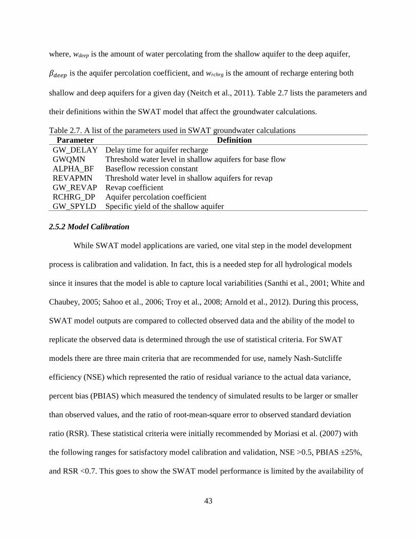
43

where, wdeep is the amount of water percolating from the shallow aquifer to the deep aquifer,

𝛽𝑑𝑒𝑒𝑝 is the aquifer percolation coefficient, and wrchrg is the amount of recharge entering both

shallow and deep aquifers for a given day (Neitch et al., 2011). Table 2.7 lists the parameters and

their definitions within the SWAT model that affect the groundwater calculations.

Table 2.7. A list of the parameters used in SWAT groundwater calculations


GW_DELAY Delay time for aquifer recharge

GWQMN Threshold water level in shallow aquifers for base flow

ALPHA_BF Baseflow recession constant

REVAPMN Threshold water level in shallow aquifers for revap

GW_REVAP Revap coefficient

RCHRG_DP Aquifer percolation coefficient

GW_SPYLD Specific yield of the shallow aquifer

2.5.2 Model Calibration

While SWAT model applications are varied, one vital step in the model development

process is calibration and validation. In fact, this is a needed step for all hydrological models

since it insures that the model is able to capture local variabilities (Santhi et al., 2001; White and

Chaubey, 2005; Sahoo et al., 2006; Troy et al., 2008; Arnold et al., 2012). During this process,

SWAT model outputs are compared to collected observed data and the ability of the model to

replicate the observed data is determined through the use of statistical criteria. For SWAT

models there are three main criteria that are recommended for use, namely Nash-Sutcliffe

efficiency (NSE) which represented the ratio of residual variance to the actual data variance,

percent bias (PBIAS) which measured the tendency of simulated results to be larger or smaller

than observed values, and the ratio of root-mean-square error to observed standard deviation

ratio (RSR). These statistical criteria were initially recommended by Moriasi et al. (2007) with

the following ranges for satisfactory model calibration and validation, NSE >0.5, PBIAS ±25%,

and RSR <0.7. This goes to show the SWAT model performance is limited by the availability of

44

reliable data. Which means that hydrological model development suffers from the same issues

that monitoring water resources has.

2.5.3 Remote Sensing in Hydrological Modeling

One approach to addressing the issues of data availability and reliability for hydrological

modeling is the use of remotely sensed data (Schuurmans et al., 2003; Xu et al., 2014). As

discussed previously, remote sensing provides a source of continuous, spatially distributed data

that can be used for regional analysis. This makes remote sensing data ideal for use in

hydrological modeling. Nevertheless, there are still limitations to the use of remotely sensed data

such as the spectral, spatial, and temporal resolutions of the collected images (Lillesand et al.,

2014). However, as long as these limitations are taken into account, it is possible to develop

reliable datasets that can be incorporated into hydrological models (Xu et al., 2014). In fact in

recent years several studies have looked at the use of remotely sensed ET data in the

hydrological model calibration process (Immerzeel and Droogers, 2008; Schuurmans et al.,

2011; Qin et al., 2013; Sousa et al., 2015; Mendiguren et al., 2017). In the study by Immerzeel

and Droogers (2008) bi-weekly actual evapotranspiration (ETa) data, obtained from the Surface

Energy Balance Algorithm (SEBAL), were integrated into the calibration of a SWAT model.

This calibration process modified SWAT parameters that were related to land use soil

characteristics, groundwater, and weather (Immerzeel and Droogers, 2008). The results of this

study showed that the incorporation of remotely sensed data could significantly improve the

model calibration process and result in more accurate model ETa simulations (Immerzeel and

Droogers, 2008). In the study by Schuurmans et al. (2011) SEBAL ETa datasets derived from

data collected by two different satellites (ASTER and MODIS) were integrated into a coupled

groundwater and unsaturated zone model (MetaSWAP) to estimate soil moisture. The result of

45

this study showed that the inclusion of the remotely sensed ETa data was able to improve the

spatial simulation of soil moisture levels (Schuurmans et al., 2011) This not only shows how

remotely sensed data could improve the modeling process but also the interconnected nature of

the hydrological cycle. In the study by Sousa et al. (2015) an ETa dataset based on MODIS

imagery was developed and incorporated into a SWAT model. The results of this integration

showed that by adding the remotely sensed ETa, the SWAT model had improved streamflow

estimates, especially in ungagged catchments (Sousa et al., 2015). This again shows that the

addition of remotely sensed data in the model calibration process is quite beneficial. In the study

by Mendiguren et al. (2017) remotely sensed ETa was used to improve the simulation of

spatially distributed ETa. Results from this study indicated that the use of remotely sensed ETa

was able to improve model simulations of the spatially distributed ETa for the region

(Mendiguren et al.; 2017). This again highlights the benefits of including remotely sensed data in

hydrological model development. All of these studies show that the incorporation of remotely

sensed data can improve the overall hydrological model performance. However, very few studies

consider a multi-objective calibration approach during the model calibration phase. Instead, most

studies focus on a single component of the hydrological model during the calibration process

(Immerzeel and Droogers, 2008; Schuurmans et al., 2011; Sousa et al., 2015; Mendiguren et al.;

2017). However, studies that have considered several hydrological components during the

calibration process indicate that adding a multi-objective calibration can improve overall model

performance and reduce the uncertainty associated with the final models (Crow et al., 2003;

Rajib et al., 2016; Franco and Bonumá, 2017) However, no studies compare the applicability of

different calibration techniques when performing a multi-objective calibration. This shows that

there is a need to perform further research in this area.

46

2.6 Modeling Uncertainty

While hydrological models and remote sensing data allow for region-wide analysis and

monitoring, it is important to note that these techniques have increased levels of error and

uncertainty compared to monitoring stations. These errors and uncertainties are often grouped

into three main categories, namely data uncertainty, model structure uncertainty, and parameter

uncertainty (Jin et al., 2010; Brigode et al., 2012; Zhang et al., 2016). The following sections

describe these categories in more detail.

2.6.1 Data Uncertainty

Data uncertainty is a way to quantify the amount of noise within a dataset (Jin et al.,

2010). This can be caused by a variety of sources from environmental factors to the limitations

of data collection equipment (Benz et al., 2004). This can have a major impact on models since

they are dependent on the quantity and quality of input data. And any noise or uncertainty within

the dataset will be passed into the model outputs as the data is used in different calculations. This

is of particular importance to remotely sensed data, which needs to account for noise from

sources such as surface properties (topographic variability and land surface directional

reflectance properties), atmospheric effects (spatial and temporal variations), and sensor design

(spectral, spatial, and radiometric properties) (Kustas and Norman, 1996; Friedl et al., 2001;

Long et al., 2014). For example, when considering remotely sensed evapotranspiration datasets,

uncertainty caused by variability surface properties (landcover type) could result in inaccurate

evapotranspiration datasets, which would increase the uncertainty of any hydrological model that

uses this evapotranspiration dataset as an input (Long et al., 2014; Yang et al., 2015). One way to

address this would be to perform accuracy assessments by comparing the evapotranspiration

products to different land-based evapotranspiration station data for different landcover types. In

47

fact, several studies have focused solely on this task (Kim et al., 2012; Senay et al., 2014; Xia et

al., 2015; Bhattarai et al., 2016). The results of these studies provide a look into the overall

accuracy of different remotely sensed evapotranspiration datasets. This allows researchers,

policy makers, and stakeholders to make educated decisions about which datasets to use for

further analysis based on their own ranges of acceptable uncertainty.

2.6.2 Model Structure Uncertainty

Model structure uncertainty is a way to quantify a model’s robustness and structure

(Brigode et al., 2012). Due to the complexity of natural systems, simplifications are used to

streamline models. However, it is possible to oversimplify a model, which increases uncertainty

associated with it by ignoring key factors and interconnected processes within the environment

(Refsgaard et al., 2006; Qin et al., 2013). In fact, this has been identified by many studies as a

major source of uncertainty (Usunoff et al., 1992; Dubus et al., 2003; Linkov and Burmistrov,

2003; Brigode et al., 2012). However, it is often challenging to reduce this uncertainty without

developing a new model. Refsgaard et al. (2006) reviewed a variety of strategies for assessing

model structure uncertainties and proposed a six-step protocol to examine conceptual

uncertainty. These steps are: 1) formulate a conceptual model; 2) set up and calibrate the model;

3) repeat steps 1 and 2 until a sufficient number of conceptual models were developed; 4)

perform validation tests and accept/reject models; 5) evaluate the tenability and completeness of

remaining conceptual models; and 6) make model predictions and assess uncertainty (Refsgaard

et al., 2006). This approach allows researchers to select the best model possible for each study

and insure that the model used captures the necessary processes of the system being modeled.

48

2.6.3 Parameter Uncertainty

Parameter uncertainty is used to describe how well model parameter values perform

when simulating model outputs (Brigode et al., 2012). However, minimizing this uncertainty is

often challenging since hydrological models require a large number of parameters to simulate the

complexity of hydrological systems. To address this, model calibration is the first step in model

development in which parameter values are altered in an attempt to better improve the model’s

ability to represent the conditions in the area of study. The calibration process compares

simulated model outputs to observed data and uses statistical analysis to determine how close the

datasets are to each other (Immerzeel and Droogers, 2008; Golmohammadi et al., 2014). Within

hydrological modeling, three statistical criteria are often used to determine if a model was

successfully calibrated, namely Nash-Sutcliffe model efficiency coefficient (NSE), root-mean-

squared error-observations standard deviation ratio (RSR), and percent bias (Pbias) (Moriasi et

al., 2007). However, while NSE, RSR, and Pbias can be used to determine if the calibration was

successful; knowing which parameters need to be changed provides a unique challenge of its

own. One way to address this would be to perform a sensitivity analysis on the model’s

parameters. This can be done through different software packages such as SWAT-CUP, which

allows modelers to perform sensitivity analysis, calibration, validation, and uncertainty analysis

of SWAT models based on Sequential Uncertainty Fitting (SUFI2), Particle Swarm Optimization

(PSO), Generalized Likelihood Uncertainty Estimation (GLUE), Parameter Solution (ParaSol),

and Markov Chain Monte Carlo (MCMC) procedures (Abbaspour, 2007). By using SWAT-CUP,

it is possible to identify which parameters should be altered as well ensure that the calibration

process was successful at reducing the model output uncertainties. Another aspect of parameter

uncertainty is equifinality, which describes the case in which a model calibration process

49

identifies multiple parameter sets that yield similar model performances (Lu et al., 2009; Jin et

al., 2010). And while this is expected to occur within hydrological modeling calibration (Beven,

1996; Savenije, 2001), it can still impact a model’s usefulness. One approach that can help

reduce the impact of equifinality within hydrological models is the complexity of the objective

function, since as objective functions become more comprehensive the chance of having multiple

calibrations performing the same is reduced (Abbaspour, 2007). By quantifying and minimizing

parameter uncertainties, model performance can be improved, which in turn results in better

model outputs for researchers, policymakers, and stakeholders.

2.7 Summary

Overall, advancements in remote sensing technology have resulted in a wide variety of

satellite-based sensors that have greatly improved our ability to monitor the Earth’s surface. And

recent years have seen an increase in the amount of research that utilizes remotely sensed data. In

particular, the field of hydrological modeling can be greatly improved by the incorporation of

satellite data and the subsequently developed remotely sensed datasets. However, while studies

have already shown the benefits of the incorporation of this data in the area of model calibration;

few studies have expanded the use of remotely sensed data to multi-objective model calibration.

Furthermore, conducting studies that explore the impacts of remotely sensed data on different

multi-objective hydrological model calibration techniques will advance the field of hydrological

modeling and allow for the development of models that more accurately simulate the real world.

50

3. INTRODUCTION TO METHODOLOGY AND RESULTS

This thesis is in the form of three research papers. The first paper, entitled “Evaluating the

Role of Evapotranspiration Remote Sensing Data in Improving Hydrological Modeling

Predictability” explores the use of remotely sensed evapotranspiration data in hydrological

modeling. As the global demands for the use of freshwater resources continue to rise, it has

become increasingly important to ensure the sustainability of this resource. This is accomplished

through the use of management strategies that often utilize monitoring and the use of

hydrological models. However, monitoring at large scales is not feasible and therefore model

applications are becoming challenging, especially when spatially distributed datasets, such as

evapotranspiration, are needed to understand the model performances. Due to these limitations,

most of the hydrological models are only calibrated for data obtained from site/point

observations, such as streamflow. Therefore, the main focus of this paper is to examine whether

the incorporation of remotely sensed and spatially distributed datasets can improve the overall

performance of the model. In this study, actual evapotranspiration (ETa) data was obtained from

the two different sets of satellite-based remote sensing data. One dataset estimates ETa based on

the Simplified Surface Energy Balance (SSEBop) model while the other one estimates ETa

based on the Atmosphere-Land Exchange Inverse (ALEXI) model. The hydrological model used

in this study is the Soil and Water Assessment Tool (SWAT), which was calibrated against

spatially distributed ETa and single point streamflow records for the Honeyoey Creek-Pine

Creek Watershed, located in Michigan, USA. Two different techniques, multi-variable (NSGA-

II) and genetic algorithm, were used to calibrate the SWAT model. Using the aforementioned

datasets, the performance of the hydrological model was evaluated by calculating Nash-Sutcliffe

51

efficiency (NSE), percent bias (PBIAS), and root mean squared error-observations standard

deviation ratio (RSR).

The second paper, entitled “Evaluating the Spatial and Temporal Variability of Remote

Sensing and Hydrologic Model Evapotranspiration Products” evaluates the spatial and temporal

performance of eight ETa datasets. Advances in satellite technology have led to the availability

of global remote sensing datasets that can be used to supplement gaps in observed hydrological

data. However, it is often challenging to identify the right dataset for different spatial and

temporal scales. Therefore, the goal of this paper is to statistically explore the spatial and

temporal performance of remotely sensed ETa datasets in a region that lacks observed data. The

remotely sensed datasets were further compared with ETa results from a physically-based

hydrologic model to examine the differences and describe discrepancy among them. All of these

datasets were compared through the use of Generalized Least-Square estimations that compared

ETa datasets on temporal (i.e., monthly and seasonal basis) and spatial (i.e., landuse) scales at

both watershed and subbasin levels.

In the third paper, entitled “Evaluation of a Many-Objective Optimization Technique to

Improve the Performance of a Hydrologic Model Using Evapotranspiration Remote Sensing

Data”, we combine streamflow and remotely sensed evapotranspiration data for hydrological

model calibration with the goal of identifying the improvement level achieved by introducing

spatially explicit data. This is similar to the first study; however, while the first study was limited

to just two objective functions (multi-objective) in the calibration process, this study selected an

improved technique that allows many-objective (more than two objective functions) calibration.

Furthermore, while the first study considered two evapotranspiration datasets (ALEXI and

SSEBop), this study considers eight evapotranspiration datasets, namely: the USGS Simplified

52

Surface Energy Balance (SSEBop), the USDA/NASA Atmosphere-Land Exchange Inverse

(ALEXI), the MODIS Global Evapotranspiration Project (MOD16A2) 500m, the MOD16A2 1

km, the North American Land Data Assimilation Systems 2 Evapotranspiration (NLDAS-2)

Mosaic, the NLDAS-2 Noah, the NLDAS-2 VIC, and finally TerraClimate. In addition to these

datasets, an Ensemble was also developed and used. Regarding the calibration processes, the

Non-dominated Sorting Genetic Algorithm, the Third Version (NSGA-III) was linked to SWAT)

to preform ten different calibrations. A total of 18 SWAT parameters were considered during

calibrations that impact the model outputs in regard to both streamflow and evapotranspiration.

The first eight calibrations utilized a multi-objective approach and used observed streamflow and

an evapotranspiration dataset as the objective functions. The ninth calibration was another multi-

objective calibration utilizing observed stream flow and the evapotranspiration Ensemble. And

finally, the tenth calibration was a many-objective calibration utilizing observed stream flow and

all of the evapotranspiration datasets. Again, NSE, Pbias, and RSR were used as the statistical

calibration criteria and a measure of the overall model performance.

53

4. EVALUATING THE ROLE OF EVAPOTRANSPIRATION REMOTE SENSING

DATA IN IMPROVING HYDROLOGICAL MODELING PREDICTABILITY

4.2 Introduction

As extreme climate conditions and anthropogenic activities continue to impact

environmental systems, mitigation and restoration related projects have become common.

Furthermore, environmental systems, such as watersheds, are very complex with many

relationships and interlocking processes (Sivakumar and Singh, 2012; Guerrero et al., 2013).

Therefore, it can be challenging to determine which management solution(s) should be selected

and implemented (Herman et al., 2015; Sabbaghian et al., 2016). This has led to the development

of many different modeling techniques that can simulate a variety of options and identify the best

solution(s), based on the criteria put forth mostly by stakeholders and policy makers (Chen et al.,

2012; Beven and Smith, 2014; Giri et al., 2016).

Meanwhile, the first step in a model implementation is parameter calibration. Parameter

calibration in model applications is used to adjust model performance to better simulate the

natural systems they are trying to describe (Guerrero et al., 2013; Zhan et al., 2013; Rajib et al.,

2016). While parameter calibration improves the ability of models to more accurately represent

natural systems, models’ performances are still limited by the quality and quantity of input data

and their availabilities (Nejadhashemi et al., 2011). Today, most hydrological studies rely on

data collected at monitoring stations across the world. In fact, the United States Geological

Survey (USGS) has about 1.5 million monitoring sites from which data can be obtained (USGS,

2016a). However, even with the existence of all these monitoring sites, there are times where

higher spatial resolutions are needed by researchers, stakeholders, and policymakers to more

precisely evaluate the hydrologic conditions and to determine the best place to implement

54

mitigation and restoration projects (Wanders et al., 2014). One way to address this issue is the

use of remotely sensed data. Remote sensing is defined as the science of identifying, observing,

and measuring an object without physical contact (Graham, 1999). With the advancements in

satellite technology, remotely sensed satellite data has become a source of consistent monitoring

for the entire globe, with applications ranging from crop yields to water resources assessments

(Graham, 1999; Long et al., 2014).

In order to model water resources more accurately, it is important to examine different

components of the hydrologic cycle, including water movement processes (e.g., evaporation and

streamflow) and water storage (e.g., soil moisture, water vapor, groundwater, and surface water

bodies). While hydrological models simulate all components of the hydrological cycle,

streamflow is often the only component that the model outputs are compared against during the

calibration process since it can be measured more accurately than the other components

(Immerzeel and Droogers, 2008; Wanders et al., 2014; Rajib et al., 2016). This can result in poor

simulations of other hydrologic components, which ultimately lowers the model performance

(Wanders et al., 2014; Rajib et al., 2016). Therefore, including additional hydrological

components in the parameter calibration process could allow the model to better represent all

process occurring in the environment (Crow et al., 2003). In particular, evapotranspiration (ET)

could be considered an important hydrological component added to the calibration process since

it describes the moisture lost to the atmosphere from both biotic (e.g., plants) and abiotic (e.g.,

soils) sources (Hanson, 1991; USGS, 2016d). Meanwhile, ET plays a major role in the cycling of

water from land and ocean surface sources into the atmosphere, which in turn drives

precipitation (Pan et al., 2015). Furthermore, Immerzeel and Droogers (2008) found that

calibrating a hydrological model for ET significantly improved ET simulations; and that ET

55

simulation values were more sensitive to groundwater and meteorological parameters compared

to soil and landuse parameters.

This indicates that including additional parameters in a model calibration can improve the

overall model performance. However, the applicably of different calibration techniques has not

been explored when both remotely sensed ET and streamflow data are involved. In addition, this

study is unique in the sense that the performance of a hydrologic model for estimating

streamflow was evaluated using different remotely sensed ET products. Therefore, the objectives

for this paper are to (1) determine the performance of a calibrated hydrologic model in

estimating ET against spatially distributed time series ET products obtained from remote

sensing; (2) determine the impact of ET parameter calibration on streamflow estimation; and (3)

evaluate the performances of different calibration techniques for streamflow and ET estimations.

4.3 Materials and Methods

4.3.1 Study Area

The study area is the Honeyoey Creek-Pine Creek Watershed (Hydrologic Unit Code

0408020203), which is located within the Saginaw Bay Watershed in Michigan’s Lower

Peninsula (Figure 4.1). The US Environmental Protection Agency (EPA) identified the Saginaw

Bay Watershed as an area of concern due to the presence of contaminated soils and degradation

of fisheries within the region (EPA, 2017). These conditions were caused by the addition of both

point and non-point source pollutants from a variety of sources such as industrial waste and

agricultural runoff (EPA, 2016). The final outlet for this watershed is Lake Huron via the

Saginaw River. Out of the approximately 1,100 km2 within the Honeyoey Watershed, agriculture

is the dominant landuse (~52%) followed by forests (~23%), wetlands (~17%) and pasturelands

(~5%). The remaining land is classified as urban (~3%). The Honeyoey Creek-Pine Creek

56

watershed has been significantly altered by anthropogenic activities as evidenced by the landuse

change (agricultural lands and urban area are dominant in the region), which in turn impacts the

natural environment, especially water quality and quantity.

Figure 4.1. The study area (Honeyoey Creek-Pine Creek watershed)

4.3.2 Data Collection

4.3.2.1 Physiographic Data

Several spatial and temporal input datasets were needed to describe the study area in a

hydrological model. These datasets describe characteristics such as topography, landuse, soil

properties, climate, and crop management practices. Data from the USGS were obtained to

represent the topography of the region using their 30 m spatial resolution National Elevation

Dataset (NED, 2014). Landuse information was acquired from the 30 m spatial resolution

Cropland Data Layer developed by the United States Department of Agriculture-National

Agricultural Statistics Service (USDA-NASS) (NASS, 2012). The Natural Resources

57

Conservation Service (NRCS) Soil Survey Geographic (SSURGO) Database was used to

describe the soil properties for the region at a scale of 1:250,000 (NRCS, 2014). National

Climatic Data Center (NCDC) weather stations (two precipitation stations and two temperature

stations) were used to obtain daily precipitation and temperature data for the time span of 2003 to

2014. A widely used stochastic weather generator called WXGEN was employed (Sharpley and

Williams, 1990; Wallis and Griffiths, 1995), which is embedded in the Soil Water Assessment

Tool (SWAT), to create climate time series for other climatological records (e.g. relative

humidity, solar radiation, and wind speed) that are required for SWAT to operate (Neitsch et al.,

2011). Predefined crop management operations, schedules, and rotations were adopted from

previous studies performed in the same region (Love and Nejadhashemi, 2011; Giri et al., 2015).

Due to the limitation of SWAT in simulating up to 250 different landuse, the subwatershed map

that was provided by the National Hydrology Dataset Plus (NHDPlus) and the Michigan Institute

for Fisheries Research at a scale of 1:24,000 were modified to accommodate this limitation

(Einheuser et al., 2013).

4.3.2.2 Remote Sensing Data

In order to evaluate the role of ET remote sensing data in improving a hydrologic model

predictability, two satellite-based ET datasets were obtained for the period of 2003 to 2014 for

the study area. One dataset was created based on the Simplified Surface Energy Balance

(SSEBop) model while the other one was based on the Atmosphere-Land Exchange Inverse

(ALEXI) model.

The USGS dataset reported monthly actual evapotranspiration (ETa) using the SSEBop

model (Senay et al., 2013). ETa is limited by the amount of water present at a site since it refers

to the actual amount of water that is lost through both evaporation and transpiration (NOAA,

58

2017b). This model utilizes ET fractions derived from 1 km Moderate Resolution Imaging

Spectroradiometer (MODIS) thermal imagery collected every eight days to develop a 1 km

monthly ETa dataset for the Conterminous U.S. (Senay et al., 2013; Velpuri et al., 2013). Data

were obtained from this dataset for each subwatershed in the study area. In order to provide an

overall ETa for each subwatershed, all SSEBop’s ETa pixels within each subwatershed were

averaged with respect to the area to generate the overall area weighted ETa average values for

each month (USGS, 2016o).

The second ETa dataset is created based on the ALEXI model, which was sponsored by

the USDA and US National Aeronautics and Space Administration (NASA). The ALEXI model

utilizes remotely sensed morning land surface temperatures to determine ETa by relating the

observed change in temperature to changes in surface moisture and ETa (Anderson et al., 1997;

Anderson et al., 2007). For this study, 4 km thermal images were obtained from Geostationary

Operational Environmental Satellites (GOES) and used as to develop a daily 4 km ETa dataset

for the Conterminous U.S. (Hain et al., 2015). In order to make the second set of ETa data

comparable to the first set, the daily ETa values from the ALEXI model were averaged to create

monthly ETa values. Next, these values were averaged for each subwatershed with respect to

area.

4.3.3 Hydrological Model: SWAT

The ETa outputs of both the ALEXI and SSEBop models were used for the evaluation of

SWAT models for the study region. SWAT is a widely used, continuous-time, semi-distributed,

hydrological model that was developed by the USDA Agricultural Research Service (USDA-

ARS) and Texas A&M AgriLife Research (Texas A&M University, 2017). By taking into

account different spatiotemporal layers of information (Section 2.2.1), such as topography,

59

landuse, and climate, SWAT models are able to simulate a variety of hydrological processes,

such as runoff, sediment transport, and ET (Gassman et al., 2007). This makes it a very useful

tool for both researchers and policymakers.

4.3.4 Calibration Approaches

For this study, all of the collected physiographic data was incorporated into a SWAT

model. However, there are many default parameters in a SWAT model that represent an average

or more probable condition that may or may not be true for the region of study (Arnold et al.,

2012). Therefore, the SWAT model used in this study underwent a series of calibration and

validation processes. To do this, all observed time series data were divided into calibration (2003

to 2008) and validation (2009 to 2014) periods. This process is simply referred to as calibration

in the rest of the paper.

Three different types of model calibration were used in this study. The first was solely a

streamflow calibration. In this approach, individual SWAT parameters that influence the

streamflow calculations were tested to find their near-optimal value through the comparison of

simulated streamflows to observed streamflows. Observed streamflow data was obtained from a

USGS streamflow station on the Pine River at the outlet of the study area (USGS, 2016p). The

next two calibration approaches, multi-variable and genetic algorithm, were used to improve the

ETa estimation for the study region. For these sets of calibrations, SWAT parameters used in

ETa calculations at the subwatershed level were altered to replicate the values obtained from the

ALEXI and SSEBop ETa datasets. In order to examine the role of these remotely sensed data on

the performance of SWAT for estimating ETa, the genetic algorithm approach was used since it

is able to optimize the system for a single variable. Meanwhile, a multi-variable calibration

approach was selected to determine the impact of add ETa calibration on the SWAT model

60

performance for both ETa and streamflow estimation. Detailed descriptions of these calibration

approaches are provided below.

4.3.4.1 SWAT Parameters

As mentioned above, during the SWAT model calibration, the SWAT parameter values

were altered. The selection of these variables was done through the use of literature review and

sensitivity analysis (Woznicki and Nejadhashemi, 2012). With respect to streamflow, 15 SWAT

parameters were identified and altered during the calibration process including: baseflow

recession constant (ALPHA_BF), biological mixing efficiency (BIOMIX), maximum canopy

storage (CANMX), effective hydraulic conductivity of channel (CH_K2), Manning’s n value for

the main channel (CH_N2), moisture condition II curve number (CN2), plant uptake

compensation factor (EPCO), soil evaporation compensation coefficient (ESCO), delay time for

aquifer recharge (GW_DELAY), revap coefficient (GW_REAP), threshold water level in

shallow aquifer for base flow (GWQMN), aquifer percolation coefficient (RCHRG_DP),

threshold water level in shallow aquifer for revap (REVAPMN), available water capacity

(SOL_AWC), and surface runoff lag coefficient (SURLAG). These parameters were selected

based on the information provided by the SWAT developer (Arnold et al., 2012). Table 4.1

presents the minimum, maximum, default, and calibrated values for all of these parameters for

the Honeyoey watershed.

61

Table 4.1. Streamflow calibration parameters used in this study

Parameter Minimum Maximum Default Calibrated

ALPHA_BF 0 1 0.048 0.55

BIOMIX 0 1 0.2 0.01

CANMX 0 100 0 1

CH_k2 -0.01 500 0 65

CH_N2 -0.01 0.3 0.014 0.025

CN2 -25% 25% NA -0.22%

EPCO 0 1 1 0.37

ESCO 0 1 0.95 0.97

GW_DELAY 0 500 31 9

GW_REVAP 0.02 0.2 0.02 0.055

GWQMN 0 5000 1000 1000

RCHRG_DP 0 1 0.05 0.35

REVAPMN 0 1000 750 900

SOL_AWC 0 1 NA 20%

SURLAG 1 24 4 1

In regards to the ETa calibration, another set of 10 SWAT parameters was identified as

being influential to the ETa calculations (Neitsch et al., 2011). These included: maximum canopy

storage (CANMX), carbon dioxide concentration (CO2), soil evaporation compensation

coefficient (ESCO), fraction of maximum stomatal conductance corresponding to the second

point on the stomatal conductance curve (FRGMAX), maximum stomatal conductance (GSI),

potential evapotranspiration method (IPET), daily maximum temperature (MAX TEMP), daily

minimum temperature (MIN TEMP), vapor pressure deficit corresponding to the fraction given

by FRGMAX (VPDFR), and daily wind speed (WND_SP). However, some of these parameters

could not be altered since they were provided by either observed data or the weather generator

used in this study, including MAX TEMP, MIN TEMP, and WND_SP. In addition, since climate

change was not a factor for this study, CO2 was also not altered. Furthermore, in an attempt to

limit the impact of the ETa calibration on streamflow, any SWAT parameters already used in the

streamflow calibration, CANMX and ESCO, were also not used during the ETa calibration

process. This reduced the initial set of ETa parameters from 10 to four. Of this set of four

62

parameters, three are crop properties and have ranges of 0.001 to 0.1 for GSI, 0 to 1 for

FRGMAX, and 1.5 to 6 for VPDFR. The last parameter used in this study, IPET, indicates which

method to use when calculating potential evapotranspiration (ETp). Within SWAT three

different ETp methods are available: namely the Penman-Monteith method, the Priestley-Taylor

method, and the Hargreaves method (Neitsch et al., 2011). All three methods were included in

the ETa calibration process; however, it was found that the Penman-Monteith method produced

the best results for the study area.

4.3.4.2 Initial Streamflow Calibration

A streamflow calibration was performed to generate a base condition to which the ETa

calibrations could be compared. In order to evaluate the performance of a hydrological model,

three statistical criteria that were suggested by Moriasi et al. (2007), were used in this study. These

criteria include: 1) Nash-Sutcliffe efficiency (NSE) representing the ratio of residual variance and

observed data variance (Nash and Sutcliffe, 1970); 2) Percent bias (PBIAS) evaluating how much

larger/smaller simulated data are than their corresponding observed data (Gupta et al., 1999); and

3) Root mean squared error (RMSE)-observations standard deviation ratio (RSR), reporting the

ratio of RMSE and standard deviation of measured data (Legates and McCabe, 1999). For

evaluating the performance of a hydrologic model on simulating monthly streamflow values, NSE

values above 0.5, PBIAS values within ±25%, and RSR values below 0.7 are considered as

satisfactory (Moriasi et al., 2007). In addition, we also reported RMSE to examine the error

associated with the simulated data in which lower values represent the better model performance.

4.3.4.3 Multi-variable Calibration

A multi-variable calibration procedure, based on Monte Carlo simulation and an

evolutionary algorithm, was applied to the SWAT model using both remotely sensed ETa

63

datasets and observed streamflow from the study area. The procedure aimed to identify the

Pareto optimal frontier and the best trade-off solution.

A solution is classified as Pareto optimal (also known as non-dominated) when the value

of any objective function cannot be improved without decreasing the performance of at least one

other objective function (Chankong and Haimes, 1993; Tang et al., 2006). In multi-variable

calibration, there is at least one objective function per observed variable. For this study, the

minimization objective function (OF) for each variable (i.e. ETa and streamflow) was based on

the NSE.

1OF NSE= − (4.1)

The objective function for ETa was computed using the area weighted average of the

monthly simulated from the hydrologic model and satellite-based ETa time series for each

subwatershed, which was determined as follows:

1

1i ij

T

n

j

i

ET A ETA =

= (4.2)

where, 𝐸𝑇̅̅ ̅̅𝑗 is the average ETa for month 𝑗; 𝐴𝑇 is the total surface area of the watershed; 𝐴𝑖 is the

surface area of subwatershed 𝑖; 𝐸𝑇𝑖𝑗 is the ETa for subwatershed 𝑖 and month 𝑗; and 𝑛 is the

number of subwatersheds. Therefore, one pair of simulated-observed ETa series for the whole

watershed was obtained to determine a unique NSE for this variable. This process was not

employed for streamflow since there is only one gauging station at the outlet of the study area

(Figure 4.1).

The general outline of the multi-variable calibration, which is further explained in the

following sections, is as follows: A Monte Carlo simulation is performed to understand the

SWAT model performance for ETa and streamflow with respect to the selected calibration

64

parameters. Thus, 5,000 parameter sets were randomly generated via uniform sampling, which

were then evaluated by executing the SWAT model for each generated parameter set. The results

were used to define, if possible, narrower calibration parameter ranges, and to obtain multi-

objective scatter plots to identify preliminarily Pareto Optimal solutions. The next step consists

of the application of a multi-objective evolutionary algorithm known as the Nondominated

Sorted Genetic Algorithm II (NSGA-II) (Deb et al., 2002) to determine the optimal Pareto

population. Finally, the decision-making method known as the Compromise Programming (Deb,

2001), using a Euclidean distance metric, was employed to select the final optimal trade-off

solution from the resulting Pareto Optimal population.

4.3.4.3.1 Monte Carlo Simulation

A total of 5,000 runs for Monte Carlo simulation were performed using MATLAB®,

with randomly generated corresponding parameter sets selected from uniform distributions.

Ranges for calibration parameters were defined as follows: 0.001 to 0.1 for GSI, 0 to 1 for

FRGMAX, and 1.5 to 6 for VPDFR. A SWAT model run was executed for each parameter

combination, computing NSE for both ETa and streamflow. Dotty plots relating each OF with

parameter values were obtained to analyze parameter identifiability, and if possible, narrower

calibration ranges to be explored with the NSGA-II algorithm. Likewise, multi-objective plots

relating ETa and streamflow OF values were generated for preliminary Pareto frontiers

identification.

4.3.4.3.2 Multi-objective Evolutionary Algorithm: NSGA-II

The NSGA-II is a multi-objective genetic algorithm that has been widely used in various

disciplines and has been successfully implemented in other SWAT applications (Zhang et al.,

2010; Lu et al., 2014; Zhang et al., 2016). The NSGA-II is a population-based algorithm that is

65

comprised of a nondominated ranking process, a crowded distance calculation, an elitist selection

method, and offspring reproduction operations (Deb, 2001). For this study, a real-coded NSGA-

II with simulated binary crossover (SBX) and polynomial mutation (Baskar et al., 2015) was

applied, requiring the prior definition of distribution indexes for each operation (defined as 20

for crossover and mutation each). Other input parameters include the population size (defined as

100), the maximum number of generations as stopping criteria (defined as 50), and the mutation

probability (defined as the reciprocal of the number of calibration parameters).

4.3.4.3.3 Compromise Programming Approach

The compromise programming approach using the 𝑙2 metric (which becomes the

Euclidean distance metric) is used to select the optimal Pareto population member that is closest

to a reference point (Deb, 2001). In this case, the ideal point, which is unfeasible and is not

located on the Pareto frontier, is selected as the reference point and it is comprised by the best

objective function values (Deb, 2001). Before computing the distance between each Pareto point

and the ideal point, the objective function values are normalized employing a Euclidian non-

dimensionalization (Sayyaadi and Mehrabipour, 2012):

1

2

n

ijm

i

i

ij

j

OFOF

OF=

=

(4.3)

where, i is the index for each point in the Pareto frontier, j is the index for each OF, m is the total

number of the Pareto population, and n superscript refers to “non-dimensional”. The distance 𝑑𝑖

between each Pareto point and the ideal point, which is the 𝑙2 metric, is calculated as follows:

( )1

2

2

ideal

ij ij

N

j

l OF OF=

= − (4.4)

where, N denotes the total number of objective functions.

66

In the compromise programming approach, the point with the minimum distance metric

value is chosen as the best trade-off solution.

4.3.4.4 Genetic Algorithm Calibration

The other approach used to calibrate the SWAT models with respect to the ETa datasets

was a genetic algorithm (GA). A GA is an optimization technique that imitates biological process

to refine a population of potential solutions to identify the best final or set of final solutions

(Goldberg, 1989; Conn et al., 1991; Conn et al., 1997). For this study, a GA was used to guide ETa

calibrations by changing the values of three parameters within the SWAT model, namely GSI,

FRGMAX, and VPDFR. These are the same parameters that were modified in the multi-variable

optimization approach, and thus the same ranges were used for this optimization. With each

successive set of parameter values, a series of MATLAB® codes were used to update and run the

SWAT model (Abouali, 2017). First, the parameter values were accepted by the code, which

checked the values to the defined ranges and then applied the values to all subwatersheds within

the region. After this was completed, the code executed the SWAT model and stored the outputs

for further analysis. In summary, the SWAT model was run 904,900 times. While executing these

runs will not necessarily develop an ideal model, it will generate a landscape of how ET changes

for each subwatershed based on the specified parameters. For each set of parameter values, the

SWAT ETa outputs were compared to the ALEXI and SSEBop datasets and NSE and RMSE were

calculated for each subwatershed. The parameter set that had the largest NSE was considered to

be the best and the lowest RMSE was used as the tiebreaker. This allowed for the identification of

the best parameter values for each subwatershed, which then used to parametrize the best model

that maximizes the ETa calibration. It should be noted that this is only possible based on the

assumption that the ETa calculation for one subwatershed is not affected by the ETa calculation

67

for another subwatershed, otherwise it would not be possible to create the mosaic landscape of

parameter values used in the best model, which to the best of our knowledge has not been done in

other SWAT studies. Furthermore, after the best parameters for each subwatershed were identified

and applied within the SWAT models, the simulated ETa values were area averaged to produce a

single ETa value for the entire watershed. This set of ETa values was then used to calculate the

NSE, PBIAS, RSR, and RSME for the entire region, just like was done in the multi-variable

calibration. This was done to allow for a watershed level evaluation of the calibration approaches.

4.3.5 Statistical Analysis

To further evaluate the streamflow and ETa outputs from the calibrated models and ETa

datasets, a mixed-effects model was used to compare the mean difference between each of the

outputs (Kuznetsova et al., 2015). This process was performed twice, once for the streamflow

datasets (observed, initial streamflow calibrated model, ALEXI multi-variable calibrated model,

ALEXI genetic algorithm calibrated model, SSEBop multi-variable calibrated model, and

SSEBop genetic algorithm calibrated model) and once for the ETa datasets (ALEXI, SSEBop,

ALEXI multi-variable calibrated model, ALEXI genetic algorithm calibrated model, SSEBop

multi-variable calibrated model, and SSEBop genetic algorithm calibrated model). This allowed

for the determination of significant mean differences between the datasets with a 95%

confidence level.

4.4 Results and Discussion

4.4.1 Initial Streamflow Calibration

Daily streamflow was calibrated and validated for a 12-year period (6 years calibration and

6 years validation) from 2003 to 2014 for the region. Table 4.2 shows the NSE, Pbias, RSR, and

RSME values achieved for the calibrated model. As shown in the table, all criteria (NSE, PBIAS,

68

and RSR) are in their respective satisfactory ranges (Moriasi et al., 2007) indicating that the model

was successfully calibrated and can be used to simulate streamflow values for the region.

Furthermore, while the overall RSME was 6.522, the calibration period had a smaller RSME

compared to the validation period, indicating a better model fit during the calibration period than

the validation period. The temporal variability of observed and simulated streamflow is also

presented in Figure 4.2. Overall, the SWAT model represents the observed flow variations very

accurately.

Table 4.2. Calibration and validation criteria NSE PBIAS (%) RSR RSME

Overall (2003-2014) 0.612 -0.965 0.623 6.522

Calibration (2003-2008) 0.611 4.303 0.624 5.996

Validation (2009-2014) 0.613 -5.856 0.622 7.009

Figure 4.2. Comparison of observed and simulated daily streamflow

The results of this section present the performance of the SWAT model in replicating the

spatially distributed ETa data obtained from two remote sensing products (SSEBop and ALEXI

datasets). Table 4.3 shows the SWAT model performance for the overall, calibration, and

69

validation periods based on NSE, PBIAS, RSR, and RMSE of the ETa for the condition in which

only the streamflow calibration was performed. These calculations followed the same procedure

that was discussed in the multi-variable and GA calibration sections, in which ETa values were

area averaged across the watershed and then used to calculate watershed level statistical criteria.

When considering the entire time period, the streamflow calibrated SWAT model was able to

replicate the SSEBop ETa dataset more accurately than the ALEXI ETa dataset. This can be seen

by the fact that the statistical criteria for the SSEBop ETa were better than those for the ALEXI

ETa. Similar results were seen for the calibration and validation periods. Overall, this shows that

the SWAT model can better replicate the SSEBop ETa data compared to the ALEXI data.

Table 4.3. Statistical criteria ETa when the results from base streamflow calibrated SWAT

model was used

Period Variable/Dataset Statistical Measure

NSE PBIAS (%) RSR RMSE

Overall (2003-2014) ALEXI ETa 0.62 27.82 0.62 21.79

SSEBop ETa 0.81 -10.12 0.44 18.28

Calibration (2003-2008) ALEXI ETa 0.62 27.83 0.62 21.48

SSEBop ETa 0.81 -8.46 0.44 18.13

Validation (2009-2014) ALEXI ETa 0.62 27.80 0.61 22.10

SSEBop ETa 0.80 -11.78 0.44 18.42

4.4.2 Multi-variable Calibration

A combination of 5,000 Monte Carlo simulations and an NSGA-II evolutionary

algorithm were used to identify the Pareto frontiers for the SWAT model calibrations for both

the ALEXI and SSEBop ETa datasets. Figure 4.3 shows both the entire Monte Carlo population

as well as the Pareto frontiers identified by the NSGA-II evolutionary algorithm for each ETa

dataset. This shows that Pareto frontiers were able to be identified from the Monte Carlo

simulations run for each ETa datasets, which indicates the first phase of the multi-variable

optimization was successful for both datasets. However, the SSEBop Pareto frontier was able to

further minimize streamflow and ETa OFs compared to the ALEXI Pareto frontier. Therefore,

70

calibrating the SWAT model using the SSEBop ETa data was able to produce a more accurate

model performance. This can be seen more clearly in Figure 4.4, which shows the Pareto

frontiers for both the SSEBop and ALEXI datasets. This figure also highlights the optimal Pareto

population member selected by the compromise programming method, which shows the optimal

model calibration for each dataset. This reinforces the conclusions that the SSEBop dataset

performed better than the ALEXI dataset and achieved a model calibration that was able to better

simulate both streamflow and ET values for the entire region. In addition, the results showed that

the multi-variable calibration was able to identify a final calibrated model for each dataset that

improved both streamflow and ET simulations.

Figure 4.3. Monte Carlo populations and Pareto frontiers for a) ALEXI and b) SSEBop datasets

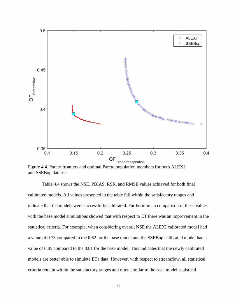
71

Figure 4.4. Pareto frontiers and optimal Pareto population members for both ALEXI

and SSEBop datasets

Table 4.4 shows the NSE, PBIAS, RSR, and RMSE values achieved for both final

calibrated models. All values presented in the table fall within the satisfactory ranges and

indicate that the models were successfully calibrated. Furthermore, a comparison of these values

with the base model simulations showed that with respect to ET there was an improvement in the

statistical criteria. For example, when considering overall NSE the ALEXI calibrated model had

a value of 0.73 compared to the 0.62 for the base model and the SSEBop calibrated model had a

value of 0.85 compared to the 0.81 for the base model. This indicates that the newly calibrated

models are better able to simulate ETa data. However, with respect to streamflow, all statistical

criteria remain within the satisfactory ranges and often similar to the base model statistical

72

criteria, suggesting that the streamflow simulations were not heavily impacted by the addition of

the ET calibration. Overall, the results show that this calibration approach was successful at

improving the models’ performances while maintaining the current streamflow accuracies.

Table 4.4. Statistical criteria for optimal multi-variable calibration models

Period ET

Dataset Statistical Criteria

NSE PBIAS (%) RSR RMSE ET Streamflow ET Streamflow ET Streamflow ET Streamflow

Overall (2003-

2014)

ALEXI 0.73 0.59 21.73 13.70 0.52 0.64 18.32 6.70 SSEBop 0.85 0.61 -

16.05 8.20 0.39 0.63 16.05 6.57

Calibration

(2003-2008)

ALEXI 0.72 0.59 22.01 18.52 0.53 0.64 18.37 6.19 SSEBop

0.85 0.61 -

14.03 12.94 0.38 0.63 15.85 6.01

Validation

(2009-2014)

ALEXI 0.74 0.59 21.46 9.22 0.51 0.64 18.28 7.18 SSEBop

0.85 0.60 -

18.07 3.79 0.39 0.63 16.25 7.09

4.4.3 Genetic Algorithm Calibration

In addition to the multi-variable approach, a GA optimization was also performed. Unlike

the multi-variable approach, this approach focused on only improving the ETa estimations for

two remotely sensed datasets (ALEXI and SSEBop) without considering the streamflow

calibration. After hundreds of runs for each subwatershed, the GA was able to identify the

optimal parameters values for each subwatershed and the ETa datasets. These final parameter

values were used to develop SWAT models that represented the optimal ETa calibration for each

subwatershed. Table 4.5 shows the NSE, PBIAS, RSR, and RMSE values achieved for both final

calibrated models. All of the ETa statistical criteria values presented in the table fall within the

satisfactory ranges and indicate that the models were successfully calibrated with respect to ET.

When compared to the base model, it can be seen that the ETa calibration performed here was

able to improve the simulation of ETa values for both the ALEXI and SSEBop datasets. For

example when considering the overall NSE, the ALEXI calibrated model had a value of 0.75

compared to the 0.62 for the base model and the SSEBop calibrated model had a value of 0.84

73

compared to the 0.81 for the base model. However, when considering the streamflow calibration,

most of the statistical values have fallen outside the satisfactory ranges (NSE > 0.5, PBIAS

±25%, and RSR < 0.7) for each criterion. This indicates that while this process was able to

improve the ET simulations, it was done at the cost of compromising streamflow simulations.

This seems logical, knowing that this approach did not consider the streamflow calibration

during the ETa calibration process. However, this does indicate that this approach would be

unsuitable for calibrating models that require accurate streamflow values.

Table 4.5. Statistical criteria for the optimal GA calibrated models Period ET

Dataset Statistical Criteria

NSE PBIAS (%) RSR RMSE ET Streamflow ET Streamflow ET Streamflow ET Streamflow

Overall (2003-

2014)

ALEXI 0.75 0.32 14.34 32.73 0.50 0.82 17.84 8.61 SSEBop 0.84 0.52 -

17.42 10.69 0.39 0.69 16/35 7.28

Calibration

(2003-2008)

ALEXI 0.74 0.22 14.89 39.24 0.51 0.88 17.82 8.50 SSEBop

0.85 0.50 -

15.25 16.22 0.39 0.71 16.19 6.80

Validation

(2009-2014)

ALEXI 0.75 0.40 13.80 26.67 0.50 0.77 17.86 8.71 SSEBop

0.84 0.53 -

19.59 5.55 0.40 0.69 16.51 7.73

4.4.4 Statistical Significance

The results of the statistical analysis of the mean difference between each of the datasets

are presented for streamflow and ETa in Tables 4.6 and 4.7, respectively. Linear mixed-effects

models were employed to account for the spatiotemporal effects that cause sample correlation

violating the independence assumption for the usual paired t-test (Esfahanian et al., 2017). With

regard to the streamflow datasets, all comparisons were found to be significantly different from

each other except for the comparison of the observed dataset with the initial streamflow

calibrated model. This indicates that the initial calibration was able to closely replicate the

observed data to the point where statistically there is no difference between them. However, the

significant difference observed for all other models compared to the observed data indicates that

74

those models are not as accurate when simulating streamflow. This seems logical for the models

calibrated via the genetic algorithm approach since there was a noticeable decrease in the

statistical criteria for the streamflow calibration in these models. However, we did not expect this

for the models calibrated using the multi-variable approach, since these models showed little to

no change in the calibration criteria for streamflow. These results indicate that even though the

calibration process was able to satisfactorily calibrate streamflow, there exist more

inconsistencies within the final simulated streamflow when compared to the observed data.

When considering the comparison of streamflow simulations between the initial model and the

other four models tested, the significant difference makes sense and indicates that the addition of

the ETa calibration influenced the streamflow calibration to an extent. Furthermore, since all of

these the p-values were negative, the ETa calibrated models all underestimated the streamflow

when compared to both the observed dataset and the initial streamflow model. This indicates that

regardless of the calibration method used or the impact seen on the statistical criteria, the ETa

calibrated models produced lower streamflow values on average. Finally, the comparisons

between the four ET calibrated models also showed a significant difference, which seems

understandable given the use of different ET datasets and calibration process used in this study.

With regards to the ETa datasets, almost all comparisons among datasets showed

significant differences except for the SSEBop dataset versus the initial streamflow calibrated

model and the SSEBop genetic algorithm calibrated model versus the ALEXI multi-variable

calibrated model. These two cases are rather interesting since the first comparison (SSEBop

versus the initial streamflow calibrated model) indicates that by only calibrating for streamflow it

was possible to simulate ETa so that it is not statistically different from the remotely sensed data.

Meanwhile the second case (SSEBop genetic algorithm calibrated model versus ALEXI multi-

75

variable calibrated model) indicates that regardless of using different approaches and datasets,

similar ETa simulations were generated. Considering all of the other significant differences, the

comparison between the ALEXI and SSEBop data made the most logical sense since different

methodologies were used to calculate these datasets. Furthermore, similar results to the

streamflow were also seen when comparing the ETa calibrated models to the remotely sensed

ETa datasets. These observations confirm that even though these models were able to

satisfactorily simulate ETa values, the SWAT simulated ETa was statistically different from the

remotely sensed data used to calibrate them, and thus could not accurately replicate the remotely

sensed data. However, while the streamflow comparisons showed that all of the ETa calibrated

SWAT models underestimated streamflow, here it can be seen that the SSEBop calibrated

SWAT models overestimated ETa values while the ALEXI calibrated SWAT models

underestimated the ETa values when compared to the SSEBop and ALEXI datasets, respectively.

In addition, similar to the streamflow comparisons, the four ETa calibrated models were

significantly different from the initial streamflow calibrated model, which makes sense since all

of the ETa calibrated models had an increase in the statistical criteria for ETa calibration

compared to the initial streamflow calibrated model. Finally, the comparisons between the four

ETa calibrated models showed a significant difference from each other except for the case of the

SSEBop genetic algorithm calibrated model versus the ALEXI multi-variable calibrated model

discussed previously. This is reasonable since different calibration approaches and ETa datasets

were used.

76

Table 4.6. Mean differences and p-values from the mixed-effects model for comparison of the different streamflow datasets used in

this study. Bolded values indicate significant difference at the 0.05 level

Streamflow

Datasets* Streamflow Datasets*

A B C D E F A B 0.08 (0.75) C -3.18 (0.00) -3.26 (0.00)

D -1.04 (0.00) -1.13 (0.00) 2.13 (0.00)

E -1.34 (0.00) -1.42 (0.00) 1.84 (0.00) -0.29 (0.01) F -0.80 (0.00) -0.89 (0.00) 2.37 (0.00) 0.24 (0.03) 0.53 (0.00)

*A = Observed Streamflow, B = Initial Streamflow Calibrated Model, C = ALEXI Genetic Algorithm Calibrated Model, D

= SSEBop Genetic Algorithm Calibrated Model, E = ALEXI Multi-Variable Calibrated Model, and F = SSEBop Multi-Variable

Calibrated Model.

Table 4.7. Mean differences and p-values from the mixed-effects model for comparison of the different ETa datasets used in this

study. Bolded values indicate significant difference at the 0.05 level

ET

Datasets* ET Datasets*

A B C D E F G A B 20.10 (0.00) C 2.75 (0.09) -17.35 (0.00) D 11.07 (0.00) -9.03 (0.00) 8.32 (0.00) E 6.69 (0.00) -13.41 (0.00) 3.94 (0.00) -4.38 (0.00) F 6.97 (0.00) -13.13 (0.00) 4.22 (0.00) -4.10 (0.00) 0.28 (0.23) G 5.67 (0.00) -14.43 (0.00) 2.92 (0.00) -5.40 (0.00) -1.02 (0.00) -1.30 (0.00)

*A = SSEBop, B = ALEXI, C = Initial Streamflow Calibrated Model, D = ALEXI Genetic Algorithm Calibrated Model, E

= SSEBop Genetic Algorithm Calibrated Model, F = ALEXI Multi-Variable Calibrated Model, and G = SSEBop Multi-Variable

Calibrated Model.

77

4.4.5 Comparison of the Multi-variable and Genetic Algorithm Calibrations

Based on the information provided in Tables 4.4 and 4.5, it can be concluded that the

multi-variable approach used in this study was able to generate better overall SWAT models

compared to the GA approach. However, if the goal of the model is to generate more accurate

ETa data, the GA approach was able to outperform the multi-variable approach. This shows that

depending on the purpose of the model applications, different calibration techniques should be

used. Furthermore, it is to be noted that for both approaches the models built using the SSEBop

data were able to achieve higher performances in simulating both streamflow and ETa data than

the models made based on the ALEXI data.

4.5 Conclusions

In this study, two different ETa calibration techniques were used to evaluate the impact

of adding spatially distributed and remotely sensed ETa datasets to the traditional streamflow

calibration used in hydrological models. Both techniques, multi-variable and GA, were able to

successfully improve the ETa calibration for the hydrological model using both remotely sensed

ETa datasets. The GA technique was able to produce better ETa calibrations and thus better ETa

simulations; however, this was achieved at the cost of lowering the streamflow calibrations.

Meanwhile, the multi-variable technique was able to improve the ETa calibration while

maintaining the streamflow calibration. Therefore, future use of these approaches should be

driven by the needs of the research. For example, if a study is focused solely on better ETa

estimation, the GA approach is the better option; meanwhile, studies focused on better

simulating the entire hydrological cycle for a region should use the multi-variable approach.

Concerning the ETa datasets used in this study, the calibrations performed with the SSEBop

dataset resulted in better ETa estimations compared to the calibrations based on the ALEXI

78

dataset for this study area. Therefore, it is recommended that future studies should perform this

analysis in other regions to better understand how these datasets compare to each other as well as

evaluating the impacts of different climate variabilities (e.g., snow cover).

Statistical analysis of the streamflow and ETa showed that the remotely sensed ETa

datasets were significantly different from each other, which was expected. Moreover, except for

one exception, all of the streamflow and ETa datasets produced by the ETa calibrated SWAT

models were also significantly different from each other. However, all four ETa calibrated

models were also significantly different when compared to the remotely sensed data. This

indicated that while the overall model calibration was successful it was unable to closely

replicate the remotely sensed data, showing that there still could be additional improvements in

the both in the calibration process and the SWAT model simulations.

It is to be noted that the ETa calibration processes used in this study only altered three

parameters within the SWAT model. This was due to temporal and computational limitations.

However, the addition of other parameters to the calibration process, such as the soil evaporation

compensation factor (ESCO), could result in even better model calibrations and thus better

model outputs and should be the focus of future studies. In addition, while adding ETa

calibration to the overall model calibration process was successful in this study, future studies

should consider additional hydrological cycle components, such as remotely sensed soil moisture

datasets. This would allow for the development of even more realistic models and thus more

accurate results for stakeholders and policymakers who rely on model outputs for managing

freshwater resources.

4.6 Acknowledgment

Authors would like to thank Dr. Wade Crow from USDA-ARS Hydrology and Remote

79

Sensing Laboratory at Beltsville, Maryland for his help with editing the paper. This work is

supported by the USDA National Institute of Food and Agriculture, Hatch project MICL02359.

80

5. EVALUATING THE SPATIAL AND TEMPORAL VARIABILITY OF REMOTE

SENSING AND HYDROLOGIC MODEL EVAPOTRANSPIRATION PRODUCTS

5.1 Introduction

Freshwater is vital for life and therefore understanding how the hydrological cycle

changes has become a major focus of many researchers, especially given the increased demand

for water across the globe (Clark et al., 2015; Srinivasan et al., 2017). Traditionally, this has been

accomplished using monitoring stations that record different aspects of the hydrological cycle,

such as streamflow and precipitation. However, these stations can be expensive to install,

maintain, and operate and thus their coverage is often low and not enough to capture spatial and

temporal variabilities of hydrological cycle especially in large areas (Wanders et al., 2014). One

solution to this is the use of remote sensing products. Remote sensing (RS) is the use of sensors

and tools to indirectly measure the characteristics of an object (Graham, 1999). And with the

advancement of satellite technology, remotely sensed has become a common approach for

generating consistent global monitoring datasets such as different elements of hydrological

cycles (Long, et al., 2014).

In the hydrological cycle, evapotranspiration (ET) is an influential component since it is

the measure of how much water enters the atmosphere from both the Earth’s surface and from

plants (USGS, 2016d). Which means that ET supplies water vapor to the atmosphere driving

weather patterns and precipitation distributions (Pan et al., 2015; USGS, 2016q). Meanwhile,

since ET measures the loss of moisture from plants and soil, its magnitude is dependent on the

landscape. Therefore, measuring ET is a large scale is difficult through traditional techniques

(Wu et al., 2008), but a prime hydrological component to be measured through remotely sensed

techniques (Anderson et al., 2012). This has led to the development of a variety of different ET

81

remotely sensed monitoring products, such as the Simplified Surface Energy Balance (SSEB)

(Zhang et al., 2016), the Atmosphere-Land Exchange Inverse (ALEXI) (Anderson et al., 2007;

Senay et al., 2013), the Moderate Resolution Imaging Spectroradiometer (MODIS) Global

Evapotranspiration Project (MOD16) (Zhang et al., 2016; NTSG, 2018), the Google Earth

Engine Evapotranspiration Flux (Google, 2018), and the North American Land Data

Assimilation Systems phase 2 (NLDAS-2) (Xia et al., 2015). These products can be categorized

based on the method they use to calculate ET with the most common categories being Surface

Energy Balance Methods, Penman-Monteith Methods, and Priestly-Taylor Methods (Bhattarai et

al., 2016; Zhang et al., 2016). However, each of these methods have different assumptions and

inputs required to calculate ET while there is a higher level of uncertainty associated with the

remotely sensed data compared to traditional ET monitoring techniques (van der Tol and Parodi,

2012; Zhang et al., 2016). All of these can make it challenging for researchers and policy makers

to know which ET product should be used considering landuse/landcover and a period of study.

One technique to address the uncertainty within remotely sensed datasets is the use of an

ensemble of several different products (Duan et al., 2007). Creating an ensemble of datasets

helps reducing the uncertainty of individual datasets by combining the benefits of each dataset

while minimizing negative aspects like outliers (Dietterich, 2000). This has led to the creation of

a variety of ensemble techniques and applications that have been applied to remotely sensed

products (Christensen and Lettenmaier, 2006; Fowler and Ekström, 2009; Lee et al., 2017; Wang

et al., 2018). The complexity of these techniques ranges from very simple calculations such as

simple averaging to very complex techniques such as ensemble Kalman filter (EnKF) (Giorgi

and Mearns, 2003; Kim et al., 2015; Wang et al., 2018). However, the Bayesian Model

Averaging (BMA) is the most commonly used ensembling technique for ET remotely sensed

82

products (Kim et al., 2015; Tian and Medina, 2017; Yao et al., 2017; Ma et al., 2018) that

reduces overall dataset uncertainty by weighting ET products based on the observed data (Kim et

al., 2015). However, this technique is dependent on the availability of observed data, which

depending on the region can be difficult to obtain.

In summary, the wide range of techniques can make it challenging to know which

technique should be applied. Therefore, given the challenges associated with the selection and

use of remotely sensed ET products in the field of hydrology three objectives were identified for

this study: 1) explore the temporal performance of individual and an ensemble remotely sensed

datasets; 2) evaluate the spatial performance of individual and an ensemble remotely sensed

datasets; 3) compare the performance of individual remotely sensed datasets to the ensemble and

hydrological model’s outputs.

5.2 Materials and Methods

To accomplish the objectives of this study a variety of tasks were performed. First eight

remotely sensed ETa datasets along with an ETa Ensemble and ETa output of a hydrological

model were obtained for a study area. Since each of these datasets has different spatial and

temporal resolutions, they were aggregated or disaggregated to create a series of comparable ETa

datasets. In order to determine their performance in the study area, several forms of statistical

analysis were performed to examine the spatiotemporal variabilities in addition to their fit to the

Ensemble and hydrological model output. The following sections provide additional information

about all of the processes used in this study.

5.2.1 Study Area

The Honeyoey Creek-Pine Creek Watershed (Hydrologic Unit Code 0408020203) was

selected for this study (Figure 5.1). Located in Michigan’s Lower Peninsula, this watershed is

83

part of the Saginaw Bay Watershed, which is the largest watershed in Michigan with the final

outlet at Lake Huron. Furthermore, this region has been identified as an area of concern by the

US Environmental Protection Agency due to the degradation of fisheries, the presence of

contaminated sediments, and implementation of fish consumption advisories within the region

(EPA, 2017). On average the region receives 81 cm of rainfall per year with higher rainfalls

observed during the months between April and November (US Climate Data, 2018).

Furthermore, the late fall and winter months (November through February) experience more

clouds and shorter days, while the late spring and summer months experience fewer clouds and

longer days. Meanwhile, the air temperature in the region ranges from -10℃ to 27℃, with winter

months (December through February) having colder temperatures and snow, while summer

months (June through August) have hotter temperatures and more rainfall (US Climate Data,

2018). Soils in the area are dominated by mixtures of loam and sand with low slopes (NRCS,

2018). Landuse in the Honeyoey watershed is dominated by agricultural land (~57%) followed

by forests (~23%), wetlands (~17%), and urban areas (~3%). Given the heavy agricultural nature

of the region is it important to note that corn and soybean rotations are the most common crops;

however, eight different cropping systems have been identified in the region including alfalfa,

corn, field peas, hay, pasture, sugar beet, soybean, and winter wheat. In general, agricultural

operations like tillage and crop planning start in mid-spring (i.e., May) and crops are harvested

mid-fall (i.e., October) (Love and Nejadhashemi, 2011). In cases where cover crops are utilized,

planting begins post-harvest in the fall, which requires additional tillage and planting operations

(Love and Nejadhashemi, 2011). Overall, 13 types of landuses were identified including: alfalfa

(ALFA), corn (CORN), field peas (FPEA), forest – deciduous (FRSD), forest – evergreen

(FRSE), hay (HAY), pasture (PAST), sugar beet (SGBT), soybean (SOYB), residential – low

84

density (URLD), urban – transportation (UTRN), wetlands – forested (WETF), and winter wheat

(WWHT) (NASS, 2018). These individual landuses were also combined into four major landuse

categories of agriculture (ALFA, CORN, FPEA, HAY, PAST, SGBT, SOYB, and WWHT),

forest (FRSD and FRSE), urban (URLD and UTRN), and wetland (WETF) for additional

analysis. Figure 5.2 shows the spatial distribution of the major landuse categories throughout the

Honeyoey watershed.

Meanwhile, regarding hydrological and climatological monitoring in the area, streamflow

is monitored by a United States Geological Survey (USGS) station located at the outlet of the

region (Figure 5.1). Furthermore, two precipitation and two temperature National Climatic Data

Center (NCDC) stations are located within the Honeyoey watershed (NCDC, 2018) (Figure 5.1).

Automated airport weather stations are also located within and around the Honeyoey watershed

and collect wind speed and direction, temperature, dew point, altimeter setting, density altitude,

visibility, sky condition, cloud ceiling, precipitation, and precipitation type (FAA, 2018).

Additional weather stations from the MSU Enviroweather system measure air and soil

temperature, precipitation, relative humidity, wind speed and direction, solar radiation, leaf

wetness, and potential ET (Enviroweathrer, 2018). However, none of the enviroweather stations

are located within the study region. Meanwhile, there are several AmeriFlux stations located in

Michigan that can be used to report ETa; however, the closest of these stations is 116 km from

the Honeyoey watershed (AmeriFlux, 2018).

85

Figure 5.1. Map of the Honeyoey watershed and locations of climatological stations within and

near the region

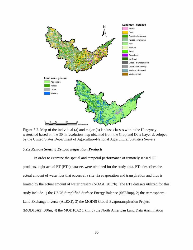
86

Figure 5.2. Map of the individual (a) and major (b) landuse classes within the Honeyoey

watershed based on the 30 m resolution map obtained from the Cropland Data Layer developed

by the United States Department of Agriculture-National Agricultural Statistics Service

5.2.2 Remote Sensing Evapotranspiration Products

In order to examine the spatial and temporal performance of remotely sensed ET

products, eight actual ET (ETa) datasets were obtained for the study area. ETa describes the

actual amount of water loss that occurs at a site via evaporation and transpiration and thus is

limited by the actual amount of water present (NOAA, 2017b). The ETa datasets utilized for this

study include 1) the USGS Simplified Surface Energy Balance (SSEBop), 2) the Atmosphere-

Land Exchange Inverse (ALEXI), 3) the MODIS Global Evapotranspiration Project

(MOD16A2) 500m, 4) the MOD16A2 1 km, 5) the North American Land Data Assimilation

87

Systems 2 Evapotranspiration (NLDAS-2) Mosaic, 6) the NLDAS-2 Noah, 7) the NLDAS-2

Variable Infiltration Capacity (VIC), and finally 8) TerraClimate.

The first ETa dataset (SSEBop) was obtained from the USGS and calculates monthly

ETa by using the simplified surface energy balance model (Senay et al., 2013). This technique

utilizes 8-day, 1 km MODIS thermal imagery to calculate ET fractions, which are then

aggregated to develop monthly ETa values for the Contiguous United States (Senay et al., 2013;

Velpuri et al., 2013). The second ETa dataset (ALEXI) was developed as a joint project between

the United States Department of Agriculture (USDA) and the National Aeronautics and Space

Administration (NASA). In this dataset, the ETa was calculated by comparing changes in

remotely sensed surface temperatures, obtained from Geostationary Operational Environmental

Satellites (GOES), and relating that difference to surface moisture loss (Anderson et al., 2007).

This calculation is performed on a daily basis, resulting in a spatial resolution of 4 km ETa

dataset for the Contiguous United States (Hain et al., 2015). The third and fourth ETa datasets

(MOD16A2 500 m and 1 km) were developed as a joint project between NASA and the

University of Montana Numerical Terradynamic Simulation Group (NTSG, 2018). This

technique utilizes the improved ET algorithm based on the Penman-Monteith equation and takes

into account additional information such as MODIS landcover, leaf area index (FPAR/LAI), and

global surface meteorology (Mu et al. 2011; NASA, 2018a,b). The result is an 8-day 500 m and

1 km global ETa datasets (NASA, 2014). The fifth through seventh ETa datasets (NLDAS-2) are

part of the North American Land Data Assimilation System (NLDAS) project, which was jointly

worked on by the National Oceanic and Atmospheric Administration (NOAA) and the National

Centers for Environmental Prediction (NCEP) Environmental Modeling Center, NASA's

Goddard Space Flight Center, Princeton University, the University of Washington, the NOAA’s

88

National Weather Service Office of Hydrological Development, and the NOAA/NCEP Climate

Prediction Center (NASA, 2018c). NLDAS-2 calculates ETa by coupling three different land

surface models, namely the Mosaic model, the Noah model, and the VIC model (Xia et al.,

2015). The use of these models allows NLDAS-2 to take into account a variety of physical

processes/characteristics such as atmosphere interactions of water and energy, vegetation and

soil moisture heterogeneity, water and energy budgets, and rainfall-runoff and water storage (Xia

et al., 2015). The results are three ETa datasets that are calculated at both hourly and monthly

time steps at a 1/8 degree spatial resolution (Long et al., 2014). And finally, the eighth ETa

dataset (TerraClimate) was developed as a joint project between the University of Idaho, the

University of Montana, and the USDA Forest Service – Rocky Mountain Research Station. The

ETa product of TerraClimate is produced based on the one-dimensional modified Thornthwaite-

Mather climatic water-balance model (Abatzoglou et al., 2018). This results in a monthly, global

ETa dataset with a spatial resolution of 4 km (Abatzoglou et al., 2018). It should be noted that

the TerraClimate did not report any ETa values for January and February. Table 5.1 summarizes

the spatial and temporal resolutions for each of the ETa datasets.

Meanwhile, since the ETa products were obtained from remotely sensed, calibration and

validation were necessary before the products were made available to the public. This was

performed for all of the aforementioned ETa products and the levels of accuracy were also

reported in Table 5.1. As can be seen in Table 5.1, the spatial accuracy of the ETa datasets varies

between 3.65 mm/month to 30.42 mm/month. However, given not every ETa product utilized the

same measure of accuracy (root mean squared error (RMSE); root-mean-square deviation

(RMSD); mean absolute error (MAE)), it is not appropriate to compare the accuracies between

types of error measurement. However, among those ETa products that reported RMSE, the most

89

accurate are the MOD16 products followed by SSEBop and then ALEXI. Meanwhile, among the

products reporting RMSD, the most accurate is NLDAS-2: Noah, followed by NLDAS-2: VIC

and then NLDAS-2: Mosiac. However, it is important to note that these errors are based on site-

specific comparisons with observed data. This means that for any given location between two

observed sites, the actual error associated with each dataset could flux. In addition, the accuracy

level reported in Table 5.1 are not absolute errors, which mean that they can change throughout

the years and for different landuses. Given this, it is important to note that the goal of this study

is not to perform revalidation for the selected datasets but to see how the ETa datasets perform

within the study area. However, we are interested to assess how different spatial and temporal

variations are represented by each dataset while identifying the possible sources of discrepancy

among datasets. In addition, and as presented Section 2.1 of this paper, while there are many

monitoring sites within and around the study area, there is a lack of observed ETa datasets.

Therefore, in order to help to account for the uncertainty within the datasets, an Ensemble dataset

based on an averaging technique (Tebaldi and Knutti, 2007) was also created. It is important to

note that, the use of a straight average for ensembling is not as robust as other techniques such as

BMA (Krishnamurti et al., 2000); however, due to the lack of observed data in the region (Figure

5.2) it was considered as the most appropriate technique to use.

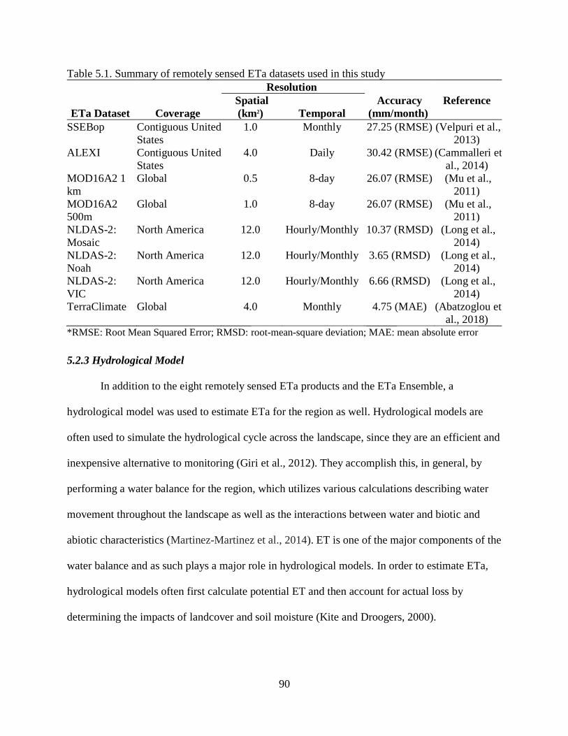
90

Table 5.1. Summary of remotely sensed ETa datasets used in this study

ETa Dataset Coverage

Resolution

Accuracy

(mm/month)

Spatial

(km2) Temporal

Reference

SSEBop Contiguous United

States

1.0 Monthly 27.25 (RMSE) (Velpuri et al.,

2013)

ALEXI Contiguous United

States

4.0 Daily 30.42 (RMSE) (Cammalleri et

al., 2014)

MOD16A2 1

km

Global 0.5 8-day 26.07 (RMSE) (Mu et al.,

2011)

MOD16A2

500m

Global 1.0 8-day 26.07 (RMSE) (Mu et al.,

2011)

NLDAS-2:

Mosaic

North America 12.0 Hourly/Monthly 10.37 (RMSD) (Long et al.,

2014)

NLDAS-2:

Noah


2014)

NLDAS-2:

VIC


2014)

TerraClimate Global 4.0 Monthly 4.75 (MAE) (Abatzoglou et

al., 2018) *RMSE: Root Mean Squared Error; RMSD: root-mean-square deviation; MAE: mean absolute error

5.2.3 Hydrological Model

In addition to the eight remotely sensed ETa products and the ETa Ensemble, a

hydrological model was used to estimate ETa for the region as well. Hydrological models are

often used to simulate the hydrological cycle across the landscape, since they are an efficient and

inexpensive alternative to monitoring (Giri et al., 2012). They accomplish this, in general, by

performing a water balance for the region, which utilizes various calculations describing water

movement throughout the landscape as well as the interactions between water and biotic and

abiotic characteristics (Martinez-Martinez et al., 2014). ET is one of the major components of the

water balance and as such plays a major role in hydrological models. In order to estimate ETa,

hydrological models often first calculate potential ET and then account for actual loss by

determining the impacts of landcover and soil moisture (Kite and Droogers, 2000).

91

In this study, the hydrological model selected was the Soil and Water Assessment Tool or

the SWAT model. SWAT is a semi-distributed, continuous-time hydrological model developed

by the USDA – Agriculture Research Service and Texas A&M AgriLife Research (Texas A&M

University, 2018). This is the most widely used hydrologic model, which utilizes several

different datasets, such as topography, soil properties, landuse, and climatological observations

to simulate hydrological parameters such as streamflow and ET (Gassman et al., 2007).

Regarding ETa estimation, the SWAT model first calculates potential evapotranspiration. This

can be done one of three ways, namely the Penman-Monteith method, the Priestley-Taylor

method, and the Hargreaves method, with the Penman-Monteith Method as the default (Neitsch

et al., 2011). After this, SWAT takes into account the evaporation from rainfall intercepted by

the canopy, maximum transpiration, maximum soil evaporation, and sublimation (during periods

of snow cover) (Neitsch et al., 2011). These calculations are performed at the hydrologic

response unit scale, which divided the region into subbasins that have unique physiographical

characteristics. For this study, 250 subbasins were created in the study area. This number was

selected due to limitations in the number of unique landuses that could be applied within the

SWAT model. Ultimately, all of these calculations result in the creation of a dataset that reports

monthly ETa at the subbasin level.

To ensure that the hydrological model represented the study area, calibration and

validation were performed for the period of 2003 to 2014, with 2003-2004 serving as a model

warmup period, 2005-2009 used for calibration period, and 2010 to 2014 used for validation

period. The hydrological cycle component used for this process was streamflow, with the daily

model streamflow output being compared to observed daily streamflow at the watershed outlet.

To evaluate this comparison, three statistical criteria were used, namely Nash-Sutcliffe efficiency

92

(NSE), percent bias (PBIAS), and root mean squared error-observations standard deviation ratio

(RSR), which were identified by Moriasi et al. (2007). Calibration and validation were successful

for the developed model since the following ranges for each statistical criterion were met: NSE >

0.5, PBIAS ±25, and RSR < 0.7 (Herman et al., 2015).

5.2.4 Remotely Sensed Actual Evapotranspiration Data Source and Conversion Procedure

All the ETa datasets were obtained for the period 2003-2014 for the study area. This

period was selected since all of the selected ETa datasets had data available during this period.

The NLDAS-2 datasets (from Mosaic, Noah and VIC models) were obtained using the NASA

Goddard Earth Science Data and Information Services Center website (NASA/GSFG, 2018).

ETa values for each model were extracted using the wgrib program developed by the NOAA’s

National Centers for Environmental Prediction (NOAA-NCEP, 2013). Similarly, average ETa

values from MOD16A (8-day values, 0.5 and 1 km resolutions) and TerraClimate (monthly

values) datasets were obtained using the code editor of Google Earth Engine (Gorelick et al.,

2017). Missing 8-day values in MOD16A datasets were completed using multi-year averages for

either the respective week or month of the missing values (the latter when the average week

value was not available) (Mu et al. 2011). Meanwhile, averaged ETa values for the USGS

SSEBop product and the USDA-NASA ALEXI product, were obtained from a previous study

(Herman et al., 2018).

However, to compare these ETa datasets, they need to be converted to similar spatial and

temporal resolutions. The first step was to ensure that each ETa dataset was reported on a

monthly basis. For datasets already reported on a monthly basis (SSEBop, NLDAS-2, and Terra

Climate) no processing was needed. However, for datasets that reported ETa on a daily (ALEXI)

or 8-day (MOD16) basis, values within each month were summed. The second step was to

93

ensure that each ETa dataset accounted for spatial variability within the landscape. To

accomplish this the ETa datasets had to be averaged for each subbasin. This was done by using

weighted area averaging technique on all ETa datasets for each unique physiographic region

within the Honeyoey watershed. The average ETa values were obtained by resampling the raster

files to a cell size of 10 m and computing the mean value of the cells within each subbasin.

Weighted area averaging was used since it was able to address the issues of multiple pixels and

partial pixels occurring within unique physiographic regions and resulted in a single ETa value

for each subbasin. By performing these two processes, eight monthly ETa datasets at the

subbasin level were created that can be used for further analysis.

5.2.5 Statistical Analysis

In order to compare the performance of the eight datasets, Ensemble, and SWAT model

within the study region, three different statistical approaches were used. These analyses were

performed to take into account different spatial scales (subbasin, watershed), landuses (major and

individual), and temporal resolutions (overall, seasonally, and monthly).

The first statistical approach evaluated the temporal variability of the different ETa

datasets and utilized multi-pairwise comparisons to estimate the monthly mean differences

between ETa datasets, for both the whole watershed and for specific landuse types. This was

done to determine if any patterns could be found among the ETa datasets throughout the year.

Since this was done for both the entire watershed and for each landuse, a total of 18 area-

weighted ETa monthly time-series were generated for each ETa dataset (13 individual landuses,

4 major landuses, and the entire watershed). To compare these datasets, two different models

were used: 1) for overall comparisons the Generalized Least-Square (GLS) estimation with

Autoregressive model, with a lag of 1, or AR (1) was used since complete time series was being

94

compared (Fox and Monette, 2002); 2) while for monthly and seasonal comparisons the GLS

estimation with Continuous Autoregressive model with lag 1, or CAR (1) was used since

irregularly-spaced time-series were being compared (Wang, 2013). In both cases, the difference

between the two analyzed time-series was used as the response variable. Furthermore, a p-value

less than 0.05 denoted datasets that were significantly different (Nejadhashemi et al., 2012).

The second statistical approach evaluated the spatial variability of the different ETa

datasets and utilized multi-pairwise comparisons of different landuse types (including the

watershed average) for each individual ETa dataset and across all ETa datasets. By performing

both of these analyses, it is possible to evaluate the performance of individual ETa datasets in

differentiating among landuse classes as well as determine if different ETa datasets perform in a

similar manner for individual landuses. This again utilized both GLS estimation with AR (1) and

GLS CAR (1) in which area-weighted ETa monthly time-series obtained for the whole watershed

while each landuse are pairwise compared. Again, the difference between the two analyzed time-

series is used as the response variable.

Finally, for the third approach, we computed the mean difference between the ETa

datasets with respect to the Ensemble and SWAT model for each subbasin. In this case, the GLS-

AR (1) regression method was used to perform an overall comparison, which reported the mean

difference and p-value for each subbasin. As a result, a series of maps were created that

represented the spatial variation of the mean differences with respect to the Ensemble and SWAT

model ETa values.

95


5.3.1 Temporal Statistical Analysis

5.3.1.1 Monthly Analysis

5.3.1.1.1 Overall Analysis

Temporal cluster analysis was performed to determine if any of the ETa datasets

produced similar results during specific times of the year. Table 5.2 presents the mean monthly

values of each ETa dataset for the entire Honeyoey watershed as well as any similarities between

datasets with superscripted letters. When different datasets have the same superscript, it indicates

that the mean difference of the datasets is not statistically different from zero. Meanwhile, if two

datasets have different superscripts, it indicates that while each dataset is similar to another

dataset, the mean difference between them is statistically different from zero. And finally, if a

dataset has no super script, it indicates that the mean difference of that dataset and all other

datasets is statistically different from zero. As presented in Table 5.2, similarities between

datasets existed for all months, with TerraClimate (with mean monthly values ranging from 1.40

mm to 110.67 mm) sharing similarity with the greatest number of other datasets overall. This

indicates that the TerraClimate dataset serves as the middle ground between the different

datasets, which could be due to the fact that TerraClimate utilizes a water-balance approach

while the rest of the products utilize energy balances (Abatzoglou et al., 2018). In addition,

winter months, such as January and February, generally had fewer similarities between datasets,

while summer months, such as June and July, had more similarities and more clusters. It is

important to note that in the context of this text, the term “clusters” is used to describe sets of

ETa datasets for which the mean difference is significantly not different from zero. This shows

that there is a higher level of variability between the datasets in the winter months compared to

96

the summer months. This could be due to the challenges related to estimating ETa when snow

cover and winter storms affect the region (Wang et al., 2015). Meanwhile, when considering the

Ensemble dataset (with mean monthly values ranging from 9.41 mm to 115.59 mm), similarities

with other datasets were seen for nine months out of the year (January, March, April, June, July,

August, September, October, and December), with August showing the most similarity with five

datasets identified as similar to the Ensemble. However, there was no consistent pattern for

which datasets were found to be similar from month to month. This may be caused by the variety

of ETa calculation techniques used for the ETa products in the study, such as surface energy

balances and water balances. Another interesting comparison is between the MOD16A2 1 km

(with mean monthly values ranging from 15.12 mm to 100.06 mm) and MOD16A2 500 m (with

mean monthly values ranging from 10.72 mm to 130.74 mm) datasets. While these two datasets

are based on the same model, they were only found to be similar for only four months out of the

year (January, February, March, and October). This is likely due to the fact that the 500 m

dataset captures more of the landscapes spatial variability compared to the 1 km dataset.

Regarding similarities between datasets throughout the year, no noticeable patterns were seen.

This is likely due to the fact that each of the ETa datasets utilize different equations, approaches,

and spatial resolutions. Another possible cause for the lack of patterns among the ETa datasets is

the fact that this analysis is the summary over the entire watershed, and patterns found within

specific landuses could be lost due to data aggregation at the watershed level.

5.3.1.1.2 Landuse Analysis

In order to determine if patterns among the ETa datasets were lost due to aggregation at

the watershed scale, monthly analysis was also performed for the major landuses (agriculture,

forest, urban, and wetland) as well as all of the individual landuses (ALFA, CORN, FPEA,

97

FRSD, FRSE, HAY, PAST, SGBT, SOYB, URLD, UTRN, WETF, WWHT). Tables S5.1, S5.2,

S5.3, and S5.4 in the Appendix showing the mean monthly values of each ETa dataset for

agricultural, forest, urban, and wetland regions, respectively, with clusters identified with

superscript letters. Meanwhile, Tables S5.5 to S5.17 in the Appendix show the same analysis for

each individual landuse.

Regarding agricultural regions (Table S5.1), similar results to the watershed scale

analysis were obtained. Winter months had more unique datasets and fewer clusters while

summer months had more clusters and fewer unique datasets. Furthermore, the TerraClimate

dataset (with mean monthly values ranging from 1.39 mm to 110.83 mm), on average, was found

to be similar to more datasets. Meanwhile, the Ensemble (with mean monthly values ranging

from 9.34 mm to 115.56 mm) was found to be similar to datasets more often when considering

agricultural areas compared to the entire watershed, with eleven of the twelve months showing

similarity to the datasets. Among all of the datasets the Ensemble was found to be similar to the

SWAT model output the most with four months out of the year (March, April, November,

December), followed by a three-way tie between MOD16A2 500m (April, May, June), NLDAS-

2: VIC (June, July, August), and TerraClimate (March, August, September). SSEBop, ALEXI,

and NLDAS-2: Mosaic were similar to the Ensemble for only two months each (July, August),

(August and October), and (January, March) respectively; while NLDAS-2: Noah was similar

only during August. While these results do not produce a distinctive pattern for individual ETa

datasets, the general increase in the number of similarities found in the months between March

and August does line up with the region’s growing season. This may indicate that the presence of

vegetation and fairer weather results in more agreement among the datasets.

98

When considering forest regions (Table S5.2), the pattern of fewer clusters and more

unique ETa datasets in the winter and more clusters and fewer unique ETa datasets in the

summer was not as apparent, though January and February still had the most unique ETa datasets

and fewest clusters. Meanwhile, all ETa datasets showed similarity with the Ensemble for at least

one month, with June showing the greatest number of similarities with five of the eight datasets

showing similarity. This is still aligned with the general pattern seen at the watershed scale

analysis. Furthermore, this pattern also matches the pattern seen for agricultural lands, in which

the months during which canopy vegetation is present, in general, show more clustering and less

variance. This may indicate the presence of vegetation improves ETa dataset convergence.

While, weather conditions could still impact this finding, the fact that forest lands had more

winter similarities than agricultural lands combined with the presence of evergreen forests that

remain vegetated year-round makes this a possible conclusion. This is further supported by

Tables S5.8 and S5.9, deciduous and evergreen forests, respectively, for which in the winter

months Table S5.9 (evergreen forests) showed more similarities than in Table S5.8 (deciduous

forests). Considering all of this, the importance of the presence of vegetation should be explored

in further studies.

Regarding urban regions (Table S5.3), again the pattern of a high number of clusters

during the growing season and fewer during the winter months was observed; however, the

pattern was less prominent. Given the observations that the presence of vegetation plays a role in

the number of clusters, this makes sense since urban regions tend to have fewer plants and more

impervious surfaces such as roads and buildings. However, when considering the number unique

ETa datasets across the span of the year, more datasets showed similarity, especially in the

winter months. This could be caused by the fact that urban regions experience less seasonal

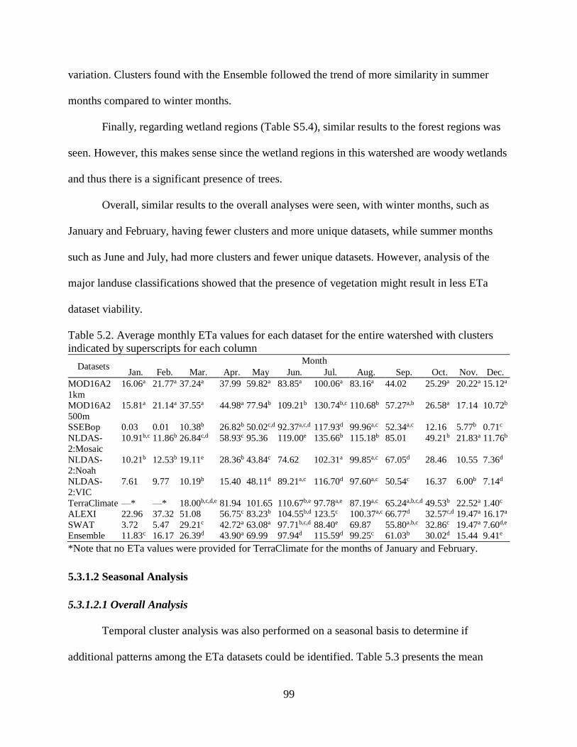
99

variation. Clusters found with the Ensemble followed the trend of more similarity in summer

months compared to winter months.

Finally, regarding wetland regions (Table S5.4), similar results to the forest regions was

seen. However, this makes sense since the wetland regions in this watershed are woody wetlands

and thus there is a significant presence of trees.

Overall, similar results to the overall analyses were seen, with winter months, such as

January and February, having fewer clusters and more unique datasets, while summer months

such as June and July, had more clusters and fewer unique datasets. However, analysis of the

major landuse classifications showed that the presence of vegetation might result in less ETa

dataset viability.

Table 5.2. Average monthly ETa values for each dataset for the entire watershed with clusters

indicated by superscripts for each column

Datasets Month

Jan. Feb. Mar. Apr. May Jun. Jul. Aug. Sep. Oct. Nov. Dec.

MOD16A2

1km

16.06a 21.77a 37.24a 37.99 59.82a 83.85a 100.06a 83.16a 44.02 25.29a 20.22a 15.12a

MOD16A2

500m

15.81a 21.14a 37.55a 44.98a 77.94b 109.21b 130.74b,c 110.68b 57.27a,b 26.58a 17.14 10.72b

SSEBop 0.03 0.01 10.38b 26.82b 50.02c,d 92.37a,c,d 117.93d 99.96a,c 52.34a,c 12.16 5.77b 0.71c

NLDAS-

2:Mosaic

10.91b,c 11.86b 26.84c,d 58.93c 95.36 119.00e 135.66b 115.18b 85.01 49.21b 21.83a 11.76b

NLDAS-

2:Noah

10.21b 12.53b 19.11e 28.36b 43.84c 74.62 102.31a 99.85a,c 67.05d 28.46 10.55 7.36d

NLDAS-

2:VIC

7.61 9.77 10.19b 15.40 48.11d 89.21a,c 116.70d 97.60a,c 50.54c 16.37 6.00b 7.14d

TerraClimate —* —* 18.00b,c,d,e 81.94 101.65 110.67b,e 97.78a,e 87.19a,c 65.24a,b,c,d 49.53b 22.52a 1.40c

ALEXI 22.96 37.32 51.08 56.75c 83.23b 104.55b,d 123.5c 100.37a,c 66.77d 32.57c,d 19.47a 16.17a

SWAT 3.72 5.47 29.21c 42.72a 63.08a 97.71b,c,d 88.40e 69.87 55.80a,b,c 32.86c 19.47a 7.60d,e

Ensemble 11.83c 16.17 26.39d 43.90a 69.99 97.94d 115.59d 99.25c 61.03b 30.02d 15.44 9.41e

*Note that no ETa values were provided for TerraClimate for the months of January and February.

5.3.1.2 Seasonal Analysis

5.3.1.2.1 Overall Analysis

Temporal cluster analysis was also performed on a seasonal basis to determine if

additional patterns among the ETa datasets could be identified. Table 5.3 presents the mean

100

monthly seasonal values of each ETa dataset for the entire Honeyoey watershed as well as any

similarities between datasets with superscripted letters. During winter, the majority of the data

sets were found to be unique with only two clusters identified, SSEBop (0.25 mm/month) and

TerraClimate (1.09 mm/month) and Mosaic (11.51 mm/month) and the Ensemble (12.47

mm/month), respectively. Regarding spring, only two datasets were found to be unique

(MOD16A2 500 m (53.49 mm/month) and VIC (24.56 mm/month)) and four clusters were

identified (MOD16A2 1 km (45.02 mm/month), SWAT (45.00 mm/month), and Ensemble

(46.76 mm/month); SSEBop (29.07 mm/month) and Noah (30.44 mm/month); Mosaic (60.38

mm/month) and ALEXI (63.68 mm/month); and TerraClimate (68.60 mm/month) and ALEXI

(63.68 mm/month)). For summer, two datasets were identified as unique (Mosaic (123.28

mm/month) and ALEXI (109.47 mm/month)) and four clusters were found (MOD16A2 1km

(89.02 mm/month), Noah (92.26 mm/month), TerraClimate (98.55 mm/month), and SWAT

(85.33 mm/month); SSEBop (103.42 mm/month), VIC (101.17 mm/month), and TerraClimate

(98.55 mm/month); SSEBop (103.42 mm/month), VIC (101.17 mm/month), TerraClimate (98.55

mm/month), and Ensemble (104.26 mm/month); and SSEBop (103.42 mm/month), TerraClimate

(98.55 mm/month), and Ensemble (104.26 mm/month)). And finally, for fall, four of the ten

datasets were unique (MOD16A2 1km (29.84 mm/month), Mosaic (52.02 mm/month),

TerraClimate (45.76 mm/month), and ALEXI (39.60 mm/month)) and three clusters were

identified (MOD16A2 500m (33.66 mm/month), Noah (35.35 mm/month), and SWAT (36.04

mm/month); SSEBop (23.42 mm/month) and VIC (24.30 mm/month); Noah (35.35 mm/month),

SWAT (36.04 mm/month), and Ensemble (35.50 mm/month)). This is similar to the monthly

analysis, in which winter and fall show fewer clusters and more unique datasets and spring and

summer show more clusters and fewer unique datasets. This is likely due to challenges such as

101

cloud cover and snow cover that occur during the fall and winter seasons (Wang et al., 2015).

Meanwhile, unlike the monthly analysis, the Ensemble showed similarities for all seasons,

though again no noticeable pattern was seen in which datasets were found to be similar.

Table 5.3. Average seasonal ETa values for each dataset for the entire watershed with clusters

indicated by superscripts for each column

Datasets Seasons

Winter Spring Summer Fall

MOD16A2 1km 17.65 45.02a 89.02a 29.84 MOD16A2 500m 15.89 53.49 116.88 33.66a SSEBop 0.25a 29.07b 103.42b,c,d 23.42b NLDAS-2:Mosaic 11.51b 60.38c 123.28 52.02 NLDAS-2:Noah 10.03 30.44b 92.26a 35.35a,c NLDAS-2:VIC 8.17 24.56 101.17b,c 24.30b TerraClimate 1.09a 68.6d 98.55a,b,c,d 45.76 ALEXI 25.48 63.68c,d 109.47 39.60 SWAT 5.6 45.00a 85.33a 36.04a,c Ensemble 12.47b 46.76a 104.26c,d 35.50c

5.3.1.2.2 Landuse Analysis

Similar to the monthly analysis, major landuse and individual landuse seasonal analysis

was performed to determine if patterns among the ETa datasets were lost due to aggregation at

the watershed scale. Tables S5.18 through S5.21 show the mean seasonal values of each ETa

dataset for agricultural, forest, urban, and wetland regions, respectively, with clusters identified

with superscript letters. Meanwhile, Tables S5.22 to S5.34 in the Appendix show the same

analysis for each individual landuse.

The results of the seasonal analysis for agricultural lands (Table S5.18) shows more

incidences of similarity compared to the overall analysis. In particular, this is true for the winter

and fall seasons. In fact, for agricultural lands fall showed the greatest number of clusters with

four clusters and only one unique ETa dataset (ALEXI (39.77 mm/month)). Meanwhile, winter,

spring, and summer all had three clusters and winter showed the most unique ETa datasets. All

of this indicates that for agricultural lands there is more agreement among the ETa datasets at the

102

seasonal level. However, while there is more agreement, there is still a lack of a pattern between

the seasons. This is likely due to the various spatial resolutions (ranging from 0.5 km2 to 12.0

km2) and governing equations (e.g., Penman-Monteith, energy balance, water balance) used for

the individual ETa products.

When considering the forest regions within the Honeyoey watershed at the seasonal level,

more unique ETa datasets were found compared to agricultural lands (Table S5.19). However,

the number of clusters for each season was identical to the agricultural lands. This is similar to

the results found in the monthly analysis. However, the matching number of clusters per season

with the agricultural regions shows that, at the seasonal scale, the fall season plays an important

role in converging ETa datasets. However, this doesn’t line up with the analysis from the

monthly section; but this could be explained by the fact that coniferous trees remain green year-

round and that deciduous trees maintain canopy cover into the middle of the fall season.

When considering the seasonal analysis for the urban areas (Table S5.20), even more

unique ETa datasets were identified than for the forest and agricultural lands. This indicates that

there is more disagreement between the different ETa datasets regarding the calculation of ETa

in urban regions. This matches the pattern seen with the monthly analysis and supports the

observation that the presence or lack of vegetation plays a major role in ETa dataset agreeance.

However, the spring and summer seasons still showed more similarities than the fall and winter

seasons. This matches the pattern found in the monthly analysis, which indicates that seasonal

weather changes affect ETa dataset performance. In addition, the summer season showed the

greatest number of similarities among the ETa datasets and the Ensemble. This also matches the

results observed in the monthly analysis.

103

Finally, when considering only wetlands regions with in the study area (Table S5.21), the

results seemed to be a mix of the agricultural and forest regions. The spring and fall seasons

showed the fewest number of unique ETa datasets (NLDAS-2: VIC (24.63 mm/month) and

ALEXI (39.20 mm/month), respectively) followed by summer (MOD16A2 500m (124.38

mm/month), NLDAS-2: Mosaic (117.63 mm/month), and SWAT (77.87 mm/month)) and then

winter (MOD16A2 1km (18.65 mm/month), MOD16A2 500m (15.58 mm/month), NLDAS-2:

Noah (9.87 mm/month), NLDAS-2:VIC (8.38 mm/month), ALEXI (25.09 mm/month), and

SWAT (6.22 mm/month)). This mixture of agricultural and forest results is interesting given the

nature of the wetland regions, which are covered in both grasses and trees. Meanwhile, the

summer season showed the greatest number of similarities with the Ensemble. This again follows

the pattern seen for the other landuse and monthly analysis.

Overall, the seasonal analysis showed similar results to the monthly analysis. This

confirmed that the presence of vegetation plays a major role in the similarity between ETa

datasets. Furthermore, spring and summer tended to show more similarities among the ETa

datasets, while the fall and winter tended to have fewer similarities and more unique ETa

datasets. This matches the weather patterns found in the region and confirms that cloud cover

and snow played a major role in ETa dataset variance. Meanwhile, there did not seem to be any

noticeable patterns amongst ETa dataset similarities between the months and seasons. This is

likely due to the various accuracies and spatial resolutions associated with the individual ETa

products. However, across the different landuses, ETa datasets tended to show similar patterns

for specific months and seasons. This is likely due to similarities in how the different ETa

datasets were calculated, for example, Noah, Mosaic, SSEBop and ALEXI all utilize forms of

104

surface energy balances to calculate ETa while MOD16A2 and SWAT utilize Penman-Monteith

techniques, and VIC and TerraClimate utilize water balances.

5.3.2 Spatial Statistical Analysis

The spatial statistical analysis was performed on the ETa datasets, Ensemble, and SWAT

model outputs to determine how the different datasets performed across different landuses. The

first step in this analysis was to determine how the individual datasets performed across the

different landuses found in the study area. This would highlight different landuses that generated

similar ETa values as well as those landuses that produced unique ETa values for each ETa

dataset. After this, a comparison among the different datasets was performed in order to

determine if any of the datasets showed similarities across different landuses.

5.3.2.1 Landuse Distinction within each ETa Dataset

5.3.2.1.1 Overview of Landuse Distinction within each ETa Dataset

Table 5.4 presents the overall datasets averages with respect to the major landuse

categories as well as the watershed scale average. Similarities between these regions are

indicated with superscript letters. As can be seen, the MOD16A2 1 km dataset only showed

similar ETa values between forest (47.81 mm/month) and wetland (47.58 mm/month) areas,

which makes sense given the nature of these landuses and could be explained by the accuracy

(1.25mm/month) of the MOD16A2 1 km product. However, when looking at the MOD16A2

500m dataset, no similarities are seen. In fact, this is the only dataset to have this result.

However, this is also the dataset with the highest resolution, which means it is better able to

capture spatial variability across the landscape. The SSEBop dataset showed the same pattern as

the MOD16A2 1 km dataset. This is interesting since both of these datasets reported ETa at 1 km

resolutions, which could explain the similarity, especially since the SSEBop accuracy is 27.9

105

mm/month compared to the 1.25 mm/month for the MOD16A2 1 km dataset. The NLDAS-2

Mosaic dataset showed similarity between agriculture (62.60 mm/month), forest (61.09

mm/month), and urban (63.28 mm/month) regions. This is interesting since these regions are

considered to be quite different from each other especially in regard to vegetation cover. This

could be caused by either the aggregation of landscape data to the 12 km2 scale used by the

NLDAS-2 datasets, the 6 mm/month accuracy, or the energy balance used to simulate ETa

values for these landuses. When considering the NLDAS-2 Noah model, a clear distinction

between agriculture (42.68 mm/month), urban (43.89 mm/month), and wetland (41.29

mm/month) areas is seen. However, forest (40.71 mm/month) regions were reported as similar to

all of the other landuses. This again could be due to issues with dataset resolution or it could

indicate that despite the improvements made in the NLDAS-2 Noah model (Xia et al., 2015) the

dataset, in some regions, still faces challenges differentiating forest regions from other landuses.

The NLDAS-2 VIC dataset had two clusters. The first showed the similarity between agriculture

(40.14 mm/month) and wetland (40.37 mm/month) areas, which matches the pattern seen for the

MOD16A2 1km and SSEBop products; while the second cluster indicated similarity between

urban (41.30 mm/month) and wetland (40.37 mm/month) regions. This again is interesting since

urban areas and wetlands are considered to be different. However, this may be due to the spatial

resolution of the NLDAS-2 datasets or the 6.66 mm/month accuracy associated with the VIC

product. Meanwhile, the TerraClimate product also showed two clusters. However, this time the

first cluster included agricultural (66.72 mm/month), forest (66.61 mm/month), and wetland

(66.70 mm/month) regions, while the second cluster included forest (66.61 mm/month) and

urban (67.01 mm/month) regions. While, the first set of similarities could be considered similar

due to the high level of vegetation present and explained by the accuracy of 4.75 mm/month; the

106

second set of similarities makes less sense. However, TerraClimate was the only ETa product

that solely utilized a water balance approach with a spatial resolution of 4 km2, which could

explain the similarity seen here. Considering the ALEXI product, one cluster of similarities was

seen between agricultural (59.66 mm/month), forest (59.77 mm/month), and wetland (59.39

mm/month) regions. This is similar to the TerraClimate product and could be explained by the

presence of vegetation. However, this may also indicate that the 4 km2 spatial resolution and

30.15 mm/month accuracy may prevent the ALEXI product from differentiating amongst

different types of vegetation in this region. Meanwhile, the SWAT model output showed two sets

of similar ETa values. The first is for agricultural (43.50 mm/month) and forest (41.45

mm/month) regions, while the second was between agriculture (43.50 mm/month) and (44.68

mm/month) wetland areas. This matches other ETa products that found different vegetated

landcovers to be similar, which in the case of SWAT is likely the results of how the SWAT

model calculates canopy cover and ETa from this surface (Neitsch et al., 2011). However, this

could also be due to the aggregation of landuses at the subbasin level, since wetlands and forests

are often surrounded by agricultural lands in the region. Finally, when considering the dataset

Ensemble, the same pattern as the MOD16A2 1 km and SSEBop products was seen, with forest

(50.30 mm/month) and wetlands (50.39 mm/month) being considered as similar. This could be

explained by the fact that both landuses have tree cover. However, this was also a common

paring amongst all of the datasets and given that the Ensemble is the average of all of the

datasets it makes sense that this similarity would also be reported for this dataset. Overall, a

number of similarities were identified. However, these could be caused by similarities in the

landuses due to changes throughout the year. Therefore, the seasonal and monthly analysis was

considered to further examine these similarities and determine their cause.

107

Table 5.4. Overall dataset averages for each major landuse category with clusters indicated by

superscripts for each column

Landuse

Dataset

MOD16A2

1 km

MOD16A2

500m SSEBop

NLDAS-

2:Mosaic

NLDAS-

2:Noah

NLDAS-

2:VIC TerraClimate ALEXI SWAT Ensemble

Agriculture 43.92 52.60 37.89 62.60a 42.68a 40.14a 66.72a 59.66a 43.50a,b 49.39

Forest 47.81a 59.30 40.89a 61.09a,b 40.71a,b,c 37.24 66.61a,b 59.77a 41.45a 50.30a

Urban 41.68 49.48 35.40 63.28a,b 43.89b 41.30b 67.01b 56.83 34.25 48.46

Wetland 47.58a 58.00 40.97a 59.85 41.29c 40.37a,b 66.70a 59.39a 44.68b 50.39a

5.3.2.1.2 Seasonal Overview of Landuse Distinction within each ETa Dataset

To determine if the similarities noticed in the overall analysis were related to specific

times of the year, the seasonal analysis was performed for each dataset, with the results presented

in Tables 5.5 and S5.35 through S5.43. This analysis was also performed on a monthly basis for

the major landuse classes (Tables S5.44 to S5.53) and for individual landuses (Tables S5.54 to

S5.63) with the results presented in the Appendix.

Tables 5.5 and S5.35 show the seasonal landuse comparisons for the MOD16A2

products. When considering the 1 km dataset (Table 5.5), forest (30.74 mm/month) and wetland

(30.53 mm/month) regions were identified as similar in the fall season, while forest (18.02

mm/month) and urban (17.98 mm/month) regions were found to be similar in the winter. The

forest and wetland similarity match the overall comparison found in Table 5.4 and could be

explained by the fact that both forest and wetlands in this region have trees which lose their

leaves in the fall as well as the accuracy of the dataset (1.25 mm/month). However, the similarity

between forest and urban regions in the summer was not seen in the overall analysis. This

indicates that the distinction of winter clusters was lost at the overall yearly analysis. These

clusters also indicate that the MOD16A2 1 km datasets should not be used to differentiate

between forest and urban regions in the winter and forest and wetland regions in the fall with

respect to ETa. Meanwhile, the spring and summer seasons showed no similar ETa values among

the major landuse categories. This shows that the MOD16A2 1 km datasets is able to identify

108

between landuses for half of the year. On the other hand, when considering the 500 m datasets

(Table S5.35), the same result seen in the overall analysis was reported, which means that no

similarities between landuses was seen. This was the only dataset to show this pattern, which

confirms that the higher resolution of this dataset was able to differentiate between all the

landuses for all times of the year. This makes this dataset ideal for isolating the ETa of individual

landuses within the Honeyoey watershed.

Table 5.5. Average seasonal values of the MOD16A2 1km dataset for the entire watershed and

each major landuse category for each column

Landuse Season

Winter Spring Summer Fall Agriculture 17.18 43.21 85.95 29.34 Forest 18.02a 47.86 94.63 30.74a Urban 17.98a 44.17 76.14 28.43 Wetland 18.65 47.37 93.79 30.53a

Table S36 shows the seasonal landuse comparisons for the SSEBop dataset. For which,

during the spring, summer, and fall seasons, forest (30.81 mm/month, 107.49 mm/month, and

24.80 mm/month, respectively) and wetland (30.99 mm/month, 107.57 mm/month, and 24.99

mm/month, respectively) regions were found to have similar ETa values. This matches the

overall analysis results and is likely due to the similarities in the forest and wetland landuses.

However, this also shows that this dataset is not ideal for differentiating between these landuses

for the majority of the year. Meanwhile, the spring season showed another set of similarities

between agricultural (27.87 mm/month) and urban (27.55 mm/month) regions. This makes less

sense given the nature of these landuses; however, it could be due to the dominance of

agricultural lands in this region and the placement of agricultural lands near urban centers in the

region as well as the accuracy of this dataset (27.90 mm/month). Another interesting note it the

fact that the SSEBop dataset was able to differentiate between all of the landuses during the

winter season. This is significant since winter offers the greatest challenges in calculating ETa

109

due to the lack of vegetation, increased cloud cover, and snow. Overall, the SSEBop dataset

should not be used for most of the year in this region, but it is ideal for winter landuse

distinctions.

Tables S5.37 through S5.39 show the seasonal landuse comparisons for the NLDAS-2

products, Mosaic, Noah, and VIC, respectively. Interestingly each approach had its own

strengths and weaknesses regarding the different seasons. Overall the Mosaic dataset showed the

most unique datasets throughout the year, with differentiation of all landuse classes during both

the spring and summer (Table S5.37). While the winter and fall seasons only showed similarities

between agricultural (11.28 mm/month and 51.69 mm/month, respectively) and wetland (11.55

mm/month and 51.63 mm/month, respectively) regions. These results are different from what

was seen at the overall analysis (Table 5.4), which showed similarities between agricultural,

forest, and urban regions. This shift at the seasonal level indicates that distinctions seen at the

seasonal level are lost when all the values are averaged. Overall, this shows that the Mosaic

dataset performs better at the seasonal scale especially for spring and summer seasons. Following

the Mosaic product’s performance at differentiating landuses, the Noah dataset was also able to

fully differentiate between all landuse classes during two seasons (winter and summer) (Table

S38). However, while the fall season only showed one similarity (urban (34.52 mm/month) and

wetland (34.47 mm/month)), the spring showed two similarities (agriculture (31.15 mm/month)

and forests (29.82 mm/month) and forest (29.82 mm/month) and wetland (28.63 mm/month)).

This was closer to the results seen in the overall analysis (Table 5.4), which showed that the

Noah product had difficulty distinguishing forest lands from other landuses. Finally, considering

the VIC product, only one season (spring) showed full differentiation of the landuses (Table

S5.39). However, the remaining seasons each showed one cluster among the landuses, with

110

forest (8.52 mm/month) and wetland (8.38 mm/month) in the winter, agriculture (103.17

mm/month) and wetland (102.64 mm/month) in the summer, and agriculture (24.04 mm/month),

forest (23.87 mm/month), and urban (23.64 mm/month) in the fall. Again, these roughly match

the findings from the overall analysis (Table 5.4), but also indicate that the VIC product

performs best in the spring.

Table S5.40 shows the seasonal landuse comparisons for the TerraClimate dataset. As

can be seen, the only season for which each landuse class was successfully distinguished was

spring. Meanwhile, each of the other seasons showed only one cluster of landuse ETa values;

with summer showing similarities between urban (97.91 mm/month) and wetland (97.99

mm/month) areas, fall showing similarities between agriculture (45.82 mm/month) and wetland

(45.86 mm/month) regions, and winter showing similarities between all landuse classes.

However, the lack of uniqueness in the winter makes sense since the TerraClimate dataset does

not report any values for January of February. Meanwhile, the seasonal analysis included

December, January, and February as the winter months. Therefore, the clustering of landuse

classes in winter just reaffirms that the TerraClimate product should not be used for winter ETa

values. However, it could be used successfully in the spring.

Table S5.41 shows the seasonal landuse comparisons for the ALEXI dataset, which is the

first ETa product to not have at least one season for which all landuse class could be

distinguished. Instead each season showed one cluster among the landuse classes; with winter

showing similarities between forest (24.60 mm/month), urban (25.26 mm/month), and wetland

(25.09 mm/month) regions; spring showing similarities between agriculture (63.92 mm/month),

forest (63.61 mm/month), and wetland (63.29 mm/month) areas; summer showing similarities

between forest (111.09 mm/month) and wetland (109.96 mm/month) regions; and fall showing

111

similarities between agriculture (39.77 mm/month) and forest (39.76 mm/month) lands (Table

S5.41). This is similar to the results found at the overall analysis for which agriculture, forest,

and wetland regions were found to be similar for the ALEXI product. This could be due to issues

with mixed pixels and a spatial resolution of 4 km2. However, it could also be influenced by the

fact that the ALEXI dataset also had the lowest accuracy among the ETa datasets, which could

result in more error when trying to differentiate between landuses.

Table S5.42 shows the seasonal landuse comparisons for the SWAT model dataset. The

SWAT model output showed similar results to the Mosaic and MOD16A2 products in the fact

that for both the spring and summer no similarities between landuse classes were seen.

Meanwhile, the fall and winter seasons each showed one cluster of landuses, which in this case

was agriculture (30.50 mm/month and 5.33 mm/month, respectively) and urban (30.70

mm/month and 5.27 mm/month, respectively) for both cases. This is different from the overall

analysis reported in Table 5.4, which showed urban as unique and agriculture similar to both

forest and wetland regions. The reduction in similarities in the seasonal analysis indicates that

aggregation to the overall analysis resulted in poorer performance. Overall, the SWAT model is

better able to distinguish among landuses in the spring and summer. This follows the pattern seen

earlier in the paper, where spring and summer seasons showed more similarities, which indicates

that once again the presence of vegetation plays a major role in determining ETa.

Finally, Table S5.43 shows the seasonal landuse comparisons for the Ensemble. As can

be seen, the Ensemble was able to successfully distinguish between landuses for winter, summer,

and fall. Meanwhile spring shows similarities between agriculture (46.47 mm/month) and forest

(47.01 mm/month) and forest (47.01 mm/month), urban (47.19 mm/month), and wetland (47.31

mm/month). However, the fact that the Ensemble was able to distinguish between landuses in

112

three of the seasons including winter shows that it was able to improve the overall ETa dataset

performance in regard to landuse differentiation. However, the landuse clusters seen in the

spring, indicate that the uniform weights applied in this study should be modified since the

majority (5 out of 8) of the datasets were able to distinguish between the landuses in the spring.

A summary of this analysis for all of the ETa products can be seen in Table 5.6. Overall,

breaking the spatial analysis down to the seasonal scale improved the individual ETa product

performances. This also allowed for the identification of the best seasons to use each dataset:

MOD16A2 1 km: spring and summer; MOD16A2 500 m: winter, spring, summer, fall; SSEBop:

winter; NLDAS-2 Mosaic: spring and summer; NLDAS-2 Noah: winter and summer; NLDAS-2

VIC: spring; TerraClimate: spring; ALEXI: none; SWAT: spring and summer; Ensemble: winter,

summer, and fall. This shows that the best product for landuse distinction in the Honeyoey

watershed was the MOD16A2 500 m, while the worst for the region was the ALEXI product.

Furthermore, analysis of the Ensemble showed that by averaging the ETa products it was

possible to improve the performance and differentiate among the major landuses.

113

Table 5.6. Summary of landuse and season differentiation for all ETa products used in this

study, X’s mark conditions that could be differentiated by the product

Dataset Spatial Scale Temporal Scale

Overall Winter Spring Summer Fall

MOD16A2 1 km

Agriculture X X X X X

Forest X X

Urban X X X X

Wetland X X X

MOD16A2 500 m

Agriculture X X X X X

Forest X X X X X

Urban X X X X X

Wetland X X X X X

SSEBop

Agriculture X X X X

Forest X

Urban X X X X

Wetland X

NLDAS-2: Mosaic

Agriculture X X

Forest X X X X

Urban X X X X

Wetland X X X

NLDAS-2: Noah

Agriculture X X X

Forest X X X

Urban X X X

Wetland X X

NLDAS-2: VIC

Agriculture X X

Forest X X X

Urban X X X

Wetland X X

TerraClimate

Agriculture X X

Forest X X X

Urban X X

Wetland X

ALEXI

Agriculture X X

Forest

Urban X X X X

Wetland X

SWAT

Agriculture X X

Forest X X X X

Urban X X X

Wetland X X X X

Ensemble

Agriculture X X X X

Forest X X X

Urban X X X X

Wetland X X X

114

5.3.2.2 Landuse Similarities between ETa Datasets

Statistical analysis comparing the ETa datasets was also performed regarding the entire

watershed and the major landuse categories (Table 5.7) and for all individual landuses (Table

S5.64). This is similar to the temporal analysis and was performed to determine if any

similarities existed between the ETa datasets when considering the spatial distribution of

landuses throughout the region. As can be seen in Table 5.7, a variety of datasets clusters were

identified. However, unlike the temporal analysis, several of the clusters spanned multiple

landuses. For example, the MOD16A2 1 km (43.92 mm/month, 41.68 mm/month, and 47.59

mm/month, respectively), NLDAS-2:Noah (42.68 mm/month, 43.89 mm/month, and 41.30

mm/month, respectively), NLDAS-2:VIC (40.14 mm/month, 41.30 mm/month, and 40.38

mm/month, respectively), and SWAT model (43.50 mm/month, 34.25 mm/month, and 44.68

mm/month, respectively) datasets had similar ETa values across agricultural, urban, and wetland

regions. This is interesting since each of these datasets has different accuracies and spatial and

temporal resolutions. However, the governing equations for each of these products is based on

energy balances, which could explain why they produced similar values across these landuses.

Meanwhile, the ALEXI (59.57 mm/month, 59.77 mm/month, 56.84 mm/month, and 59.39

mm/month, respectively) and TerraClimate (66.73 mm/month, 66.62 mm/month, 67.01

mm/month, and 66.70 mm/month, respectively) and the ALEXI (59.57 mm/month, 59.77

mm/month, 56.84 mm/month, and 59.39 mm/month, respectively) and NLDAS-2:Mosaic (62.61

mm/month, 61.09 mm/month, 63.28 mm/month, and 59.86 mm/month, respectively) ETa

products were similar for all major landuses. The similarity between the ALEXI and Mosaic

products can also be explained by the fact that both use energy balances to calculate ETa, which

is similar to the first cluster of ETa products. However, considering the TerraClimate/ALEXI

115

similarity, these products utilize different governing equations (water balance vs. energy

balance) and have very different accuracies. However, they share the same spatial resolution.

This in combination with the other clusters indicates that ETa product similarity can be obtained

for datasets that utilize similar approaches; however, it is also possible to achieve this same result

if datasets share a spatial resolution. However, given the spatial nature of ETa, this makes sense.

On the other hand, at the watershed scale, there was a reduction in the number of datasets

sets found to be similar, for example at the watershed scale the MOD16A2 1 km dataset (45.39

mm/month) was not considered similar to the NLDAS-2: Noah (42.03 mm/month), NLDAS-2:

VIC (39.56 mm/month), and SWAT (43.00 mm/month) datasets, which was seen when

considering specific landuses. This shows that aggregation to the watershed level can result in

the loss of similarities among ETa products, which indicates that performing analysis for specific

landuses improves overall product agreement. Overall, the presence of recurring patterns among

the ETa products when considering landuses shows that agreement among the ETa products is

possible and is influenced by spatially dependent variables such as landuse and governing

equations. This makes sense given the spatial variability associated with ETa; however, when

combined with the lack of patterns in the temporal analysis indicates that landuse plays a more

important role for ETa than seasonal variations, at least with respect to product agreement.

116

Table 5.7. Overall summary of average ETa values for each dataset for the entire watershed and

each major landuse category with clusters indicated by superscripts for each column

Dataset Region

Watershed Agricultural Forest Urban Wetlands MOD16A2 1km 45.39a 43.92a 47.82a 41.68a 47.59a,b MOD16A2 500m 54.98b 52.61b 59.30b,c 49.49b 58.00c,d SSEBop 39.05c 37.89 40.90d 35.40c 40.98a NLDAS-2:Mosaic 61.80d 62.61c 61.09b 63.28d 59.86c NLDAS-2:Noah 42.03a,c 42.68a 40.72d 43.89a 41.30a NLDAS-2:VIC 39.56c 40.14a 37.24e 41.30a,c 40.38a TerraClimate 66.71b,d 66.73b,c 66.62c 67.01e 66.70d ALEXI 59.57b,d 59.67b,c 59.77b,c 56.84d,e 59.39c,d SWAT 43.00c 43.50a 41.45d,e 34.25a,c 44.68a,b Ensemble 49.75 49.39 50.31a 48.46b 50.39b

5.3.4 Subbasin-level Statistical Analysis

5.3.4.1 SWAT Model Output

Similar to the landuse analysis performed between all of the datasets, the spatial mean

difference was also calculated between the eight remotely sensed ETa products and the SWAT

model output at the subbasin level. This analysis, presented graphically in Figure 5.3, provides a

spatial overview regarding how well the SWAT model was able to replicate the remotely sensed

ETa datasets. As can be seen in Figure 5.3, most of the subbasins in maps a), c), e), and f),

MOD16A2 1 km, SSEBop, NLDAS-2: Noah and NLDAS-2: VIC respectively, show no

difference in their ETa values with the SWAT model output. This matches the results seen in

Section 3.2.2, which also showed that these datasets were more closely aligned with the SWAT

model regarding individual landuse ETa values. However, while the previous analysis indicated

that these datasets were similar in nature, the spatial subbasin analysis shows that the SWAT

model output is over- or under-estimating different regions within the Honeyoey watershed. This

shows that while the overall analysis showed agreement, it is important to take into account

spatial variation within the landscape. On the other hand, when considering the other remotely

sensed ETa datasets, most of the region shows that the SWAT model is underestimating the

117

values reported by the MOD16A2 500 m, NLDAS-2: Mosaic, TerraClimate, and ALEXI

products. This also matches the earlier results of this study as well as the results of previous

studies that showed that the SWAT model had a better fit with the SSEBop dataset compared to

the ALEXI dataset (Herman et al., 2018). These results are further supported by subbasin level

statistical difference/no difference presented in Figure S5.1 in the Appendix.

118

Figure 5.3. Maps showing the mean difference between each ETa dataset and the SWAT model

output. Maps correspond to a) MOD16A2 1 km, b) MOD16A2 500 m, c) SSEBop, d) NLDAS-2:

Mosaic, e) NLDAS-2: Noah, f) NLDAS-2: VIC, g) TerraClimate, and h) ALEXI

5.3.4.2 Ensemble

The subbaisn level analysis was also performed comparing the Ensemble’s ETa values to

the eight remotely sensed ETa products and the SWAT model output. As can be seen in Figure

5.4, the Ensemble was either under- or overestimating ETa values for all the datasets.

119

Interestingly the split as to which datasets was under- or overestimated matched the split of those

datasets that were either similar of different from the SWAT model output. With MOD16A2 1

km, SSEBop, NLDAS-2: Noah and NLDAS-2: VIC showing that the Ensemble overestimated

Eta values, while comparisons to MOD16A2 500 m, NLDAS-2: Mosaic, TerraClimate, and

ALEXI products showed underestimation. However, this makes sense since the Ensemble was

created by averaging all datasets used in this study. This would result in a dataset that fits the

middle ground between all datasets, which is the case here. This also explains why the Ensemble

was found to be statistically different for the majority of subbasins for all datasets (Figure S5.2 in

the Appendix).

120

Figure 5.4. Maps showing the mean difference between each ETa dataset and the Ensemble.

Maps correspond to a) MOD16A2 1 km, b) MOD16A2 500 m, c) SSEBop, d) NLDAS-

2: Mosaic, e) NLDAS-2: Noah, f) NLDAS-2: VIC, g) TerraClimate, h) ALEXI, and i) SWAT

model

5.4 Conclusions

Throughout the course of this study, statistical analysis was used to compare the

performance of published remotely sensed ETa products in a region with no observed ETa data.

Overall, temporal analysis of the datasets showed that there was no noticeable trend in

similarities between specific datasets at both monthly and seasonal scales. However, a general

121

pattern was seen with summer and spring seasons showing more clusters among the datasets and

fewer unique datasets. Meanwhile, fall and winter seasons showed fewer clusters and more

unique ETa datasets. This is reflective of weather and vegetation cover trends within the region.

Nevertheless, the lack of patterns among the datasets shows that temporal variation is less

influential when compared to spatial variation. This likely due to several factors such as spatial

resolutions. This was most clearly identified in the comparison of the two MOD16A2 products

(1 km and 500 m). Despite both products utilizing the same approach and temporal resolution,

the lack of similarity throughout the year can only be attributed to the impact of different spatial

resolutions.

Meanwhile, spatial analysis at both the watershed, landuse, and subbasin levels led to the

identification of two major clusters within the ETa datasets. With higher ETa values reported by

MOD16A2 500 m, NLDAS-2: Mosaic, TerraClimate, and ALEXI; and lower ETa values

reported by MOD16A2 1 km, SSEBop, NLDAS-2: Noah, NLDAS-2: VIC, and SWAT. These

clusters were consistent across different landuses. This highlights two major points. First, there is

lots of variance among the different remote sensing ETa products, which is driven by the use of

different governing equations, spatial and temporal resolutions, and accuracies. However, the

second point is that it is possible to find similar ETa time series across different remote sensing

ETa products, this is driven by the use of similar governing equations and spatial resolutions.

However, it is important to note which datasets should be used when. Overall, the ETa

product that was able to differentiate amongst all of the major landuses for all seasons was the

MOD16A2 500 m dataset. However, all of the other datasets, except for ALEXI, were able to

differentiate between landuses for at least one season. Therefore, based on the analysis

performed in this study the recommended seasons for each ETa product are: MOD16A2 1 km:

122

spring and summer; MOD16A2 500 m: winter, spring, summer, fall; SSEBop: winter; NLDAS-2

Mosaic: spring and summer; NLDAS-2 Noah: winter and summer; NLDAS-2 VIC: spring;

TerraClimate: spring; ALEXI: none; SWAT: spring and summer; Ensemble: winter, summer,

and fall. This can also help stakeholders, policy makers, and researchers select the best ETa

dataset for different tasks such as monitoring of agricultural lands or tracking deforestation.

However, this study was performed for only one watershed; future studies should be

performed to expand this analysis to different climatological zones. This would help improve our

understanding of how each ETa product performs across the global landscape and which one

should or should not be recommended for a different time or landuse help ensure that the correct

ETa dataset is selected. Furthermore, other ensembling techniques should be performed to

identify the best for different regions.

5.5 Acknowledgment

Authors would like to thank Dr. Martha C. Anderson from USDA-ARS Hydrology and

Remote Sensing Laboratory at Beltsville, Maryland and Dr. Christopher R. Hain from NASA

Marshall Space Flight Center at Huntsville, AL for his help in providing ALEXI data. This work

is supported by the USDA National Institute of Food and Agriculture, Hatch project

MICL02359.

123

6. EVALUATION OF MULTI AND MANY-OBJECTIVE OPTIMIZATION

TECHNIQUES TO IMPROVE THE PERFORMANCE OF A HYDROLOGIC MODEL

USING EVAPOTRANSPIRATION REMOTE SENSING DATA

6.1 Introduction

Unchecked anthropogenic activities have led to the degradation of natural systems that

are vital to society and life as we know it. In particular, the impacts on the Earth’s limited

freshwater supplies in combination with the increasing demand for freshwater have made

freshwater monitoring and water resources sustainability a major focus for researchers

worldwide (Gleick, 1993; Srinivasan et al., 2017; Haddeland et al., 2014). This requires the

collection of data describing how different components of the hydrological cycle change across

space and time. Traditionally, this has been accomplished through the use of a variety of

monitoring stations, which are able to collect highly accurate measurements of different

components of the hydrological cycle (USGS, 2018). However, monitoring stations are often

expensive to install and maintain and are unable to provide the spatial resolution needed for

large-scale analysis (Wanders et al., 2014). This has led to the introduction and use of

hydrological models (Einheuser et al., 2013). Hydrological models are fast, inexpensive, and

versatile tools for researchers compared to monitoring stations. However, due to the fact that no

model can perfectly characterize all elements within a watershed, a level of uncertainty is

associated with all modeling practices (Kusre et al., 2010).

One way to improve model performance and mitigate model uncertainty is through the

use of model calibration and validation. Due to the complex nature of the hydrological cycle,

hydrological models utilize hundreds of parameters to describe the natural world, each with a

default value assigned by the model. However, the default value often does not represent the

124

real-world conditions; therefore, the parameter values need to be adjusted to improve model

performance (Rajib et al., 2016). This is accomplished by modifying the parameter values and

comparing the model output to observed data. In hydrological modeling, this is traditionally done

by comparing simulated and observed streamflows and using statistical criteria to test model

performance (Wanders et al., 2014). However, since hydrological models are used to simulate

other elements of the hydrological cycle, using just one element in the calibration process could

result in poor performances in other hydrological components, which reduces the overall model

performance (Wanders et al., 2014; Rajib et al., 2016). Therefore, it is important to consider

additional hydrological elements in the model calibration process (Crow et al., 2003). When

considering other hydrological elements, evapotranspiration (ET) stands out as an ideal addition

to model calibration, since it describes the loss of water from plants and the Earth’s surface,

which in turn drives weather patterns (Pan et al., 2015). In fact, the use of both ET and

streamflow in hydrological model calibration has been the focus of recent research, which

showed that global model performance was improved by the inclusion of ET (Herman et al.,

2018). However, while this helps mitigate model uncertainty, models are still dependent on the

quality and quantity of data available (Nejadhashemi et al., 2011).

One solution to this is the use of remotely sensed products. Remote sensing is the use of

sensors and imaging equipment to indirectly measure the characteristics of an object (Graham,

1999). Which when coupled with satellite technology has resulted in the development of many

global monitoring datasets that can be used to measure elements of the hydrological cycle (Long

et al., 2014). In particular, remote sensing has become a source of monitoring data for actual

evapotranspiration (ETa), which describes the actual loss of water from both evaporation and

transpiration (USGS, 2016d). A variety of remotely sensed ETa products have already been

125

developed including the Simplified Surface Energy Balance (SSEB) (Zhang et al., 2016), the

Atmosphere-Land Exchange Inverse (ALEXI) (Anderson et al., 2007; Senay et al., 2013), the

Moderate Resolution Imaging Spectroradiometer (MODIS) Global Evapotranspiration Project

(MOD16) (Zhang et al., 2016; NTSG, 2018), the Google Earth Engine Evapotranspiration Flux

(Google, 2018), and the North American Land Data Assimilation Systems phase 2 (NLDAS-2)

(Xia et al., 2015). Each of which has different inputs and temporal and spatial resolutions, and

methodologies, which can make it challenging to know, which product to use when.

Furthermore, it is important to note that while remotely sensing helps the issue with improving

data quantity and availability, it does not directly solve the issue of data quality.

However, one way to mitigate the uncertainty associated it remotely sensed products is

the use of ensemble techniques, which aim to combine the benefits of each product while

accounting for their limitations (Dietterich, 2000; Duan et al., 2007). Here again, a variety of

different techniques have been developed ranging from very simple calculations to complex

modeling approaches (Lee et al., 2017; Wang et al., 2018). Furthermore, some techniques require

the use of accurate observed data to determine, which remotely sensed products are more

accurate for the region of study (Kim et al., 2015).

Overall, the wide range of techniques and remotely sensed products are available for

hydrologic model calibration; however, there is lack of study on comparison among Eta remotely

sensed products on the improvement of hydrologic model performance which is the goal of this

study. Therefore, the objectives of this study are to 1) compare the performance of individual

remotely sensed ETa products and an ensemble through the use of a multi-objective calibration

process and 2) explore the use of a many-objective calibrations that takes into account multiple

remotely sensed ETa products and streamflow.

126

6.2 Methodology

6.2.1 Study Area

For this study, the Honeyoey Creek-Pine Creek Watershed (Hydrologic Unit Code

0408020203) located about the middle of the Lower Peninsula of Michigan (USA) was used to

evaluate the applicability of remote sensing products to improve the overall performance of

hydrologic models (Figure 6.1). This watershed is a part of the Saginaw Bay Watershed and has

a final outlet to Lake Huron. Covering approximately 1,100 km2, the region is predominantly

used for agriculture, with about 52% of the land devoted for crop production. After agriculture,

the next major landuse is forests (~23%), wetlands (~17%), pasturelands (~5%), and finally

urban (~3%).

This region is ideal for testing the remote sensing products since there is a lack of spatial

monitoring data in the area that can be used to setup a hydrologic model. However, streamflow is

monitored on a daily basis at the outlet of the watershed by United States Geological Survey

(USGS) station (USGS, 2016d) and National Climatic Data Center (NCDC) has two stations in

the region that measure daily precipitation and temperature (NCDC, 2018). However, there is no

data available in the watershed or its surrounding area for ETa. In fact, the closest source of

observed ETa data are the AmeriFlux stations located about 116 km away from the Honeyoey

watershed (AmeriFlux, 2018). All of this shows that remote sensing could serve a vital role in

this region by providing consistent datasets for monitoring of the hydrological conditions.

127

Figure 6.1. Map of the Honeyoey watershed

6.2.2 Hydrological Model

In order to evaluate the hydrological cycle in the Honeyoey watershed, the Soil and

Water Assessment Tool or SWAT was selected to be the hydrological model. SWAT is a

commonly used hydrological model that is time continuous and semi-distributed and was

developed by the USDA Agricultural Research Service and Texas A&M AgriLife Research

(Texas A&M University, 2017). The SWAT model is able to simulate a variety of different

hydrological process and scenarios by taking into account regional characteristics such as the

climate, topography, soil properties, and landuse (Gassman et al., 2007). Relevant to this study is

128

the way in which SWAT simulates ETa. The first step is calculating potential evapotranspiration,

which in SWAT can be done with three different techniques: 1) Penman-Monteith, 2) Priestley-

Taylor, and 3) Hargreaves. The default method selected is the Penman-Monteith Method as the

default (Neitsch et al., 2011). After calculating potential evapotranspiration, the SWAT model

takes into account evaporation and transpiration from several sources including the evaporation

from rainfall intercepted by the canopy, maximum transpiration, maximum soil evaporation, and

sublimation (during periods of snow cover) (Neitsch et al., 2011). These are calculated at the

hydrologic response unit scale, which in this study is the subbasin scale. Each subbasin has

unique physiographical characteristics, and for this study, the Honeyoey watershed was divided

into 250 subbasins, due to limitations in the number of unique landuses that could be applied

within the SWAT model. Nevertheless, by calculating the potential evapotranspiration and

taking into account the sources of evaporation and transpiration at the subbasin level, the SWAT

model is able to report monthly ETa values for the entire region.

In order to develop the SWAT model for the Honeyoey watershed, several spatial and

temporal datasets were used. This included topography, landuse, soil characteristics,

climatological conditions, and crop management practices. For regional topography, the 30 m

National Elevation Dataset from the USGS was used to calculate watershed slope (NED, 2014).

Meanwhile, 30 m landuse data was obtained from the 2012 Cropland Data Layer, which was

developed by the United States Department of Agriculture (USDA)-National Agricultural

Statistics Service (NASS, 2012). Regional soil characteristics were obtained on a scale of

1:250,000 from the Natural Resources Conservation Service (NRCS) Soil Survey Geographic

Database (NRCS, 2014). Climatological conditions (precipitation and temperature) for the period

of 2003 to 2014 were obtained from four National Climate Data Center stations (two temperature

129

and two precipitation stations) (NCDC, 2018). All other climatological conditions (e.g., wind

speed, solar radiation, and relative humidity) that are required by the SWAT model were

provided using a stochastic weather generator called WXGEN (Sharpley and Williams, 1990;

Wallis and Griffiths, 1995; Neitsch et al., 2011). Crop management practices, which included

operations, schedules, and crop rotations, were adopted from studies the utilized the SWAT

model in the same region to account for local practices (Love and Nejadhashemi, 2011). A

predefined subbasin map with a scale of 1:24,000 was obtained from the National Hydrology

Dataset Plus (NHDPlus) and the Michigan Institute for Fisheries Research and then modified to

make a layer with 250 subbasins. In order to perform the calibrations (which refers to both

calibration and validation) in this study, observed streamflow data was obtained from the Pine

River USGS station located at the outlet of the Honeyoey watershed for the period from 2003 to

2014 (USGS, 2016p). For this period the first two years (2003-2004) were used for warm-up, the

next five years (2005-2009) were used for model calibration, and the last five years (2010-2014)

were used for model validation.

6.2.4 Remote Sensing Actual Evapotranspiration Products

Given the lack of observed ETa data in the region and in order to calibrate the SWAT

model, eight different remotely sensed ETa products were obtained: 1) the USGS Simplified

Surface Energy Balance (SSEBop), 2) the Atmosphere-Land Exchange Inverse (ALEXI), 3) the

MODIS Global Evapotranspiration Project (MOD16A2) 500m, 4) the MOD16A2 1 km, 5) the

North American Land Data Assimilation Systems 2 Evapotranspiration (NLDAS-2) Mosaic, 6)

the NLDAS-2 Noah, 7) the NLDAS-2 Variable Infiltration Capacity (VIC), and finally 8)

TerraClimate. Each of these products utilizes different inputs and techniques the resulting

products have different spatial and temporal resolutions. The following is a brief overview of

130

each ETa product as well as each spatial and temporal resolution, while a summary of these

datasets is provided in Table S6.1 (Appendix).

The SSEBop ETa product was developed by the USGS and utilizes a simplified energy

balance to calculate ETa on a monthly basis for the Contiguous United States (Senay et al.,

2013). This is accomplished by calculating ET fractions from 8-day, 1 km MODIS thermal

imagery, which are then aggregated to a monthly scale (Senay et al., 2013; Velpuri et al., 2013).

The next ETa product (ALEXI) was the product of a joint project between the USDA and

the National Aeronautics and Space Administration (NASA) and is also based on an energy

balance. However, instead of ET fraction, ALEXI utilizes daily changes in surface temperature,

obtained from Geostationary Operational Environmental Satellites, and relates to surface water

loss or ETa (Anderson et al., 2007). The resulting product reports ETa on a daily time step at a 4

km spatial resolution for the Contiguous United States (Hain et al., 2015).

The next two ETa products (MOD16A2 500m and MOD16A2 1 km) utilize the same

methodology but have different spatial resolutions. These products were the result of a joint

project between NASA and the University of Montana Numerical Terradynamic Simulation

Group (NTSG, 2018). ETa is calculated by using an ET algorithm that is based on the Penman-

Monteith equation and also requires MODIS landcover, the fraction of photosynthetically active

radiation/leaf area index, and global surface meteorology (Mu et al. 2011; NASA, 2018a,b). The

results are global 8-day ETa products at 500 m or 1 km spatial resolutions depending on the

inputs used (NASA, 2014).

The next three ETa products (Mosaic, Noah, and VIC) were developed as a joint project

between National Oceanic and Atmospheric Administration (NOAA) and the National Centers

for Environmental Prediction (NCEP) Environmental Modeling Center, NASA's Goddard Space

131

Flight Center, Princeton University, the University of Washington, the NOAA’s National

Weather Service Office of Hydrological Development, and the NOAA/NCEP Climate Prediction

Center and are part of the North American Land Data Assimilation System (NLDAS) project

(NASA, 2018c). Each of the products utilizes a different land surface model to take into account

a variety of factors such as atmosphere interactions of water and energy, vegetation and soil

moisture heterogeneity, water and energy budgets, and rainfall-runoff and water storage (Xia et

al., 2015). The ETa products that result from these models report ETa at both hourly and

monthly time steps with a spatial resolution of 1/8 degree or 12 km for the entirety of North

America (Long et al., 2014).

The last ETa product (TerraClimate) utilized a water-balance model and was the result of

a joint project between University of Idaho, the University of Montana, and the USDA Forest

Service – Rocky Mountain Research Station. The water-balance model utilized by TerraClimate

is based on the one-dimensional modified Thornthwaite-Mather climatic model (Abatzoglou et

al., 2018), which resulted in a global ETa product that has a monthly time step and a 4 km spatial

resolution (Abatzoglou et al., 2018).

As discussed in the introduction, while remote sensing provides access to global spatially

distributed datasets, it also has more uncertainty associated with it. Therefore, during the

development of each of the ETa products used in this study, extensive calibration and validation

were performed based on the observed data. The accuracies of these products can also be seen in

Table S6.1. However, it is important to note that these accuracies are based on comparisons to

specific locations where observed data was available. And given the nature of ETa, these

accuracies could flux across the landscape. This means that for each dataset it may perform

better, equal, or worse in any other locations such as the Honeyoey watershed. However, it is

132

important that the goal of this study is not to perform revalidation but to explore modeling

applications of remote sensing ETa products to improve the performance of physically-based

hydrologic models in regions lacking observed data. This means that while the model

calibrations cannot confirm the best ETa product to use globally, it can highlight those that

perform better than others in a region. This can be measured by comparing the level of

improvement in the model predictability of streamflow using different ETa products since the

observed streamflow data are more available than observed ETa. Nevertheless, an ensemble of

the ETa products is also used in this study for the model calibration to help reduce the

uncertainty level associated with the ETa products. Concerning techniques for ETa product

ensembleing Bayesian Model Averaging (BMA) is the commonly used technique (Kim et al.,

2015; Tian and Medina, 2017; Yao et al., 2017; Ma et al., 2018). BMA reduces overall product

uncertainty by determining weights for each ETa product by comparing them to observed data

(Kim et al., 2015). However, when the observed data is not available, as this is the case in this

study, an averaging technique can be used (Tebaldi and Knutti, 2007).

6.2.5 Calibration Techniques

We implemented a multi-variable calibration approach in order to account for multiple

sources of information describing both streamflow and actual evapotranspiration variables. The

overall calibration process consisted in 1) processing remote sensing products to obtain monthly

ETa time series for the entire study area, 2) selecting model calibration parameters, 3) defining

objective functions for each variable, 4) formulating the multi-objective optimization problem to

solve, 5) selecting and implementing a suitable multi- and many-objective optimization

algorithms and 6) selecting the best trade-off solution for analysis purposes.

133

For this study, we implemented two different strategies in the formulation of the multi-

variable calibration process. In the first strategy, we implemented a multi-objective optimization

approach in which the preformance of a hydrological model was evaluated using individual ETa

remote sensing products while in the second strategy, we used a many-objective optimization

algorithm in order to evaluate the performance of a hydrological model when all ETa remote

sensing products were simentensinously considered used. For both strategies, we opted for

implementing optimization approaches, avoiding the subjective formulation of a single

aggregated objective function. In addition, multi- and many-objective frameworks provide a set

of optimal solutions describing the trade-offs between streamflow and ETa performances while

incorporating external sources of information describing both variables. In this study, we

employed the recently proposed evolutionary optimization algorithm – Unified Non-dominated

Sorting Genetic Algorithm III (U-NSGA-III) (Seada and Deb, 2016), which is capable of solving

different types of problems (i.e., single, multi, and many-objective). Furthermore, in order to

compare the resulting Pareto-optimal solutions, we selected the best trade-off solution by

employing the compromise programming approach. A detailed description of the calibration

approach is presented below.

6.2.5.1 Data processing

During the calibration process, the observed data consisted of eight raster-based remote

sensing products for ETa, and a unique observed streamflow daily time series from a USGS

gauging station located at the watershed’s outlet. Each remote sensing product was comprised of

a collection of images, each of those representing a snapshot of ETa over a specific time step

(from daily to monthly, depending on the dataset). For each image, we obtained the average ETa

value for each subbasin within the study area. This was done by using a weighted area averaging

134

technique for each subbasin (Srinivasan and Arnold, 1954). Weighted area averaging was used

since it was able to account for the multiple pixels and partial pixels within each subbasin. To do

this each ETa product was resampled to a cell size 10 m and then area weighted averaging was

used for all the 10 m cells within a subbasin (Brown, 2014). This resulted in a time series of

average ETa values for each subbasin. Then since the ETa remote sensing products are also

varied temporally, they were aggregated on a monthly time step for each subbasin. Finally, for

each dataset, we computed a monthly area-weighted average time series for the entire study area,

as follows:

𝐸𝑇𝑖̅̅ ̅̅ =

1

𝐴𝑇∑ 𝐴𝑤𝐸𝑇𝑤𝑖

𝑁𝑤=1 (6.1)

where, 𝐸𝑇𝑖̅̅ ̅̅ is the area-weighted ETa value of the ith monthly record, 𝐴𝑇 is the total watershed

area, 𝐴𝑤 is the area of the subbasin w, 𝐸𝑇𝑤𝑖 is the ETa value of the ith monthly record for the

subbasin w, and N is the total number of subbasins. The times series used for both streamflow

and ETa, were obtained for the period of 2003 – 2014.

6.2.5.2 Calibration parameters

Since the goal of the study is to simultaneously improve the SWAT model predictability

concerning streamflow and ETa, relevant parameters affecting these elements of the hydrological

cycle need to be identified and adjusted during the calibration process. Based on the literature

review, the SWAT model documentation, and sensitivity analysis; 18 parameters were selected

for this study (Arnold et al., 2012; Woznicki and Nejadhashemi, 2012). These parameters are:

baseflow recession constant (ALPHA_BF), biological mixing efficiency (BIOMIX), maximum

canopy storage (CANMX), effective hydraulic conductivity of channel (CH_K2), Manning’s n

value for the main channel (CH_N2), moisture condition II curve number (CN2), plant uptake

compensation factor (EPCO), soil evaporation compensation coefficient (ESCO), fraction of

135

maximum stomatal conductance corresponding to the second point on the stomatal conductance

curve (FRGMAX), maximum stomatal conductance at high solar radiation and low vapor

pressure deficit (GSI), delay time for aquifer recharge (GW_DELAY), revap coefficient

(GW_REAP), threshold water level in shallow aquifer for base flow (GWQMN), aquifer

percolation coefficient (RCHRG_DP), threshold water level in shallow aquifer for revap

(REVAPMN), available water capacity (SOL_AWC), surface runoff lag coefficient (SURLAG),

and the vapor pressure deficit corresponding to the second point on the stomatal conductance

curve (VPDFR). The minimum, maximum, and default values for all these parameters are

presented in Table 6.1.

Table 6.1. SWAT parameters considered during the model calibration and validation process

Parameter Minimum Value Maximum Value Default Value

ALPHA_BF 0 1 0.048

BIOMIX 0 1 0.2

CANMX 0 100 0

CH_K2 -0.01 500 0

CH_N2 -0.01 0.3 0.014

CN2 -25% 25% Various

EPCO 0 1 1

ESCO 0 1 0.95

FRGMAX 0 1 Various

GSI 0.001 0.05 Various

GW_DELAY 0 500 31

GW_REVAP 0.02 0.2 0.02

GWQMN 0 5000 1000

RCHRG_DP 0 1 0.05

REVAPMN 0 1000 750

SOL_AWC -25% 25% Various

SURLAG 1 24 4

VPDFR 1.5 6 Various

6.2.5.3 Objective functions

For each variable, we formulated a minimization objective function (f) based on the Nash-

Sutcliffe efficiency NSE, as follows:

136

𝑁𝑆𝐸 =∑ (𝑂𝑖−𝑃𝑖)2𝑛

𝑖=1

∑ (𝑂𝑖−�̅�)𝑛𝑖=1

2 (6.2)

𝑓 = 1 − 𝑁𝑆𝐸 (6.3)

where, 𝑂𝑖 is the ith observation of the considered variable (i.e., streamflow or ETa), �̅� is the

average of the observed data, 𝑃𝑖 is the ith simulated value of the considered variable, and n is the

total number of observations. The range of the resulting objective functions spans from zero to

infinity, where zero represents a perfect fit between simulated and observed time series. It is

worth noting that we used daily time series for streamflow, whereas for ETa, we used a monthly

time step. The monthly ETa time series obtained for each remote sensing product were

considered as the observed ETa data. For each simulation in the optimization process, we

computed only one OF for streamflow using the available observed dataset at the outlet of the

study area, and as many OF for ETa as the number of ETa datasets.

6.2.5.4 Optimization strategies

We implemented two calibration strategies to evaluate the influence of the different ETa

datasets in the prediction of daily streamflows. In the first strategy (multi-objective

optimization), we formulated several multi-objective optimization problems to simultaneously

minimize the difference between observed and simulated time series for both streamflow and

ETa. For each multi-objective problem, we used a different ETa dataset. Moreover, in this

strategy, we formulated an additional multi-objective optimization problem employing an

ensemble ETa dataset. This ensemble dataset was computed by averaging the monthly values of

the ETa time series from each individual remote sensing product. As a result, for the first

strategy we obtained as many Pareto-optimal fronts as the number of ETa datasets used in this

study. Each optimization problem was formulated as follows:

min𝜃∈Ω

𝐹(𝜃) = [𝑓𝑄(𝜃), 𝑓𝐸𝑇(𝜃)] (6.4)

137

where, F is a vector composed of multiple objective functions, 𝜃 is a vector containing values for

p model calibration parameters, 𝛺 is a p-dimensional parameter space limited by the calibration

ranges for each model parameter, 𝑓𝑄 is the objective function evaluated for streamflow, and 𝑓𝐸𝑇

is the objective function evaluated for ETa.

In the second strategy (many-objective optimization), we simultaneously minimized all the

objective functions derived from each ETa datasets and for the streamflow variable. In this

strategy, we did not include the ensemble dataset in order to avoid the addition of redundant

information into the overall optimization process. Hence, this strategy results in one Pareto-

optimal front. The many-objective optimization problem was formulated as follows:

min𝜃∈Ω

𝐹(𝜃) = [𝑓𝑄(𝜃), 𝑓𝐸𝑇1(𝜃), 𝑓𝐸𝑇2

(𝜃), … , 𝑓𝐸𝑇𝑀(𝜃)] (6.5)

where, 𝑓𝐸𝑇𝑚 is the objective function evaluated using the mth ETa dataset, and M is the total

number of ETa datasets.

6.2.5.5 Multi-objective optimization algorithm

The U-NSGA-III algorithm is an extension of the recently proposed NSGA-III algorithm

(Deb and Jain, 2014). The original NSGA-III is a population-based, elitist procedure based on

reference directions, which uses non-domination sorting and evolutionary operators (i.e.,

crossover and mutation) to move towards an optimal Pareto front. Reference directions are

vectors that evenly fill the objective space. The algorithm uses these vectors to rank the diversity

of individuals (Deb & Jain, 2014). Moreover, these vectors are normalized by default in order to

achieve an equally diverse optimal Pareto front with respect to each objective function. NSGA-

III’s parameters are the population size, the number of generations, the crossover and mutation

probabilities, and distributions indices associated with the crossover and mutation operations.

138

This algorithm has been found to reduce its performance when working with two or one

objective functions. However, by incorporating an explicit selection procedure when scaling

down to two and single-objective problems, the U-NSGA-III algorithm is capable of solving

single-, multi- (i.e. two to three objective functions) and many-objective (i.e. more than three

objective functions) optimization problems without adding extra parameters (Seada and Deb,

2016).

It is worth noting that prioritizing streamflow and ETa for the many-objective optimization

strategy described in the previous section, posed an interesting challenge. By default, U-NSGA-

III equally prioritize all the objectives. Therefore, ETa calibration holds most of the total weight

of the overall search for this strategy since here we have eight ETa remote sensing products.

Likewise, optimization under these default settings may result in a poor calibration performance

for streamflow. To improve performance, the balance of weights along each objective was

modified by manipulating reference direction vectors in order to award the same amount of

weight to the streamflow calibration objective function as all the ETa objective functions

together.

To modify the weights, the set of (M+1)-dimensional reference directions is simplified

into a two-dimensional reference direction set. The first dimension represents the weight given to

all of the M ETa objectives, and the second dimension represents the weight given to the

streamflow objective. The reference directions are created by the Das-Denis method that

generates normalized reference direction vectors (Das & Dennis, 1998). At this stage, the

reference directions can be represented in the following matrix:

[

𝑟11 𝑟12

⋮ ⋮𝑟𝑑1 𝑟𝑑2

]

139

where rxy is the yth dimension for the xth reference direction, and d is the number of reference

directions to create. Since the objectives are equally weighted according to the Das-Denis

method, the following relationship must be attained:

(𝑟𝑥1 + 𝑟𝑥2 = 1) ∀ 𝑥 (6.6)

Then, we generate a d × (M+1) reference direction matrix out of the d×2 matrix by

splitting the first dimension (representing ETa) into M different weights for each of the ETa

objective functions:

[

𝑟11𝑤1 𝑟11𝑤2 . . . 𝑟11𝑤𝑀 𝑟12

⋮ ⋮ ⋱ ⋮ ⋮𝑟𝑑1𝑤1 𝑟𝑑1𝑤2 . . . 𝑟𝑑1𝑤𝑀 𝑟𝑑2

]

where, wz is zth weight for each of the ETa objectives, such that w𝑧 ∈ ℝ , 0 ≤ w𝑧 ≤ 1. Since all

ETa datasets will be equally weighed, i.e. wz = 1/M ∀ z, and because ∑ 𝑤𝑧𝑀𝑧=1 = 1, the sum of the

elements of each row in the d × (M+1) matrix showed above must be equal to 1:

[(∑ 𝑤𝑧𝑀𝑧=1 𝑟𝑥1) + 𝑟𝑥2 = 1]∀𝑥 (6.7)

Therefore, here we developed d (M+1)-dimensional reference directions, where the first M

dimensions together have the same weight as the (M+1)th dimension. These reference directions

then used in U-NSGA-III to provide the same weight for the M objective functions for ETa as for

the streamflow objective function.

The java code is implementing the U-NSGA-III algorithms was provided by the

Computational Optimization and Innovation (COIN) Laboratory at Michigan State University.

This code was adapted for calibrating the SWAT model for this study. To the best of our

knowledge, this is the first time that the U-NSGA-III algorithm is used for hydrologic model

calibration using both streamflow and ETa remotely sensed products.

140

6.2.5.6 Best trade-off solution

In order to obtain the best trade-off calibration solution considering both streamflow and

ETa, in this study, we employed the compromise programming approach using the 𝑙2 metric

(Zeleny & Cochrane, 1973). This allows selection of an individual point from each Pareto-

optimal front attained after implementing the multi-objective optimization strategies. The metric

was computed for each member i of the Pareto front as follows:

𝑙2𝑖= √∑ (

|𝑓𝑖𝑗−𝑓𝑖𝑗𝑖𝑑𝑒𝑎𝑙|

|𝑓𝑖𝑗𝑖𝑑𝑒𝑎𝑙−𝑓𝑖𝑗

𝑛𝑎𝑑𝑖𝑟|)

2

𝑁𝑗=1 (6.8)

where, j is an index identifying each objective function f; N is the total number of Pareto-optimal

points, 𝑓𝑖𝑑𝑒𝑎𝑙 is the vector containing the ideal point coordinates, which is an unfeasible solution

located outside the Pareto front, representing the best expected objective function values (in this

case, zero); and 𝑓𝑛𝑎𝑑𝑖𝑟 is the vector containing the nadir point coordinates, which is comprised

of the worst objective function values obtained for each dimension at the optimal Pareto front.

The point with the minimum 𝑙2 metric (i.e., closest to the ideal point) is selected as the best

trade-off solution.

In addition to the best trade-off solutions of the multiple Pareto fronts, we also calculated

the worst expected solutions from a common nadir point for all the Pareto-optimal solutions. For

this purpose, we identified the individual solution (i.e., model simulation) providing the

minimum 𝑓𝑄 among all the Pareto fronts. Then, from this model solution, we computed the

corresponding 𝑓𝐸𝑇 for each of the ETa datasets (i.e., we obtained the worst expected 𝑓𝐸𝑇 for each

dataset). Thus, the nadir point was defined as the vector containing the maximum𝑓𝑄 and the

worst expected 𝑓𝐸𝑇 among all the Pareto-optimal solutions.

141

6.2.5.7 Calibration Evaluation

In order to determine how well the SWAT model replicated either the spatially

distributed remotely sensed ETa or point measurement of streamflow records at the outlet of the

watershed, three statistical criteria were used, which were recommended by Moriasi et al. (2007).

The three criteria are: 1) Nash-Sutcliffe efficiency (NSE); 2) percent bias (PBIAS); and 3) the

ratio of root-mean- square error (RMSE) to observed standard deviation ratio (RSR). NSE is a

measure of the level of residual variance compared actual measured data variance (Nash and

Sutcliffe, 1970). PBIAS is a measure of the overall simulated dataset’s tendency to be larger or

smaller than the observed data (Gupta et al., 1999). RSR is as its name implies a ratio between

the RMSE and the observed standard deviation (Singh et al., 2005). For a model to be

satisfactorily calibrated the following criteria needed to be met: NSE >0.5, PBIAS ±25%, and

RSR <0.7 (Moriasi et al., 2007).


6.3.1 Evaluation of the Performance of the Different Multi-objective Calibrations

The first goal of this study was to evaluate the improvement in performance of a

hydrological model in estimating the streamflow by comparing the potential benefit of using the

eight different ETa products along with an Ensemble of all the datasets. To do this, nine SWAT

models were calibrated by adjusting the 18 SWAT parameters that affecting both streamflow and

Eta estimation as it was discussed in Section 6.2.5.1. Each calibration had two objective

functions, 1) streamflow with observed data collected from a USGS station at the watershed

outlet and 2) ETa with each calibration using a different ETa product. This resulted in a total of 9

different calibrations, each of which had 65,100 simulations, resulting in a total 585,900

simulations across all multi-objective calibrations. The results of the NSGA-III calibrations are

142

presented in Figure 6.2 in the form of optimal Pareto frontiers. As can be seen, variability among

the ETa products resulted in a wide range of performances. However, regarding individual

models, the Ensemble ETa product showed highest overall model performance while the

TerraClimate ETa product showed the lowest overall model performance. This shows that the

Ensemble, which was used minimize the uncertainty associated with the individual ETa

products, was successful and outperformed all products. However, it is important to note that

none of the ETa products were compared to observed data, and thus the Ensemble cannot be

labeled as the most accurate of the ETa products. Instead, the Ensemble was able to most closely

replicate the SWAT model simulations. Meanwhile, since SWAT is a physically based model,

the fact that the Ensemble outperformed all the other ETa products indicates that at least for this

region, the Ensemble product is more aligned with current knowledge of water movement is a

watershed according to the hydrological cycle.

143

Figure 6.2. Comparison of the Pareto frontiers of the nine multi-objective calibrated SWAT

models

To better understand Figure 6.2 and how each calibration performed, a summary of each

set of Pareto optimal solutions for each multi-objective optimization, with respect to the NSE

statistical criteria, is presented in Table 6.2. This includes the mean, standard deviation,

coefficient of variation, minimum, maximum, the best trade-off solution, and the worst case ETa

performance. The maximum and minimum columns show the best and worst NSE values for

each objective function. Here it is important to note that all cases fall within the satisfactory

ranges for the NSE calibration criteria. This means that all of the potential solutions identified by

the calibration process in the Pareto frontiers would be considered as acceptable models.

However, the ETa model performance was higher than the streamflow performance, showing

that the calibration process had a better fit in replicating the ETa products than the observed

144

streamflow. However, in this study, the best or optimal solutions to each calibration are

presented in the “Best Trade-off” column. These cases were calculated as the solution that had

the smallest distance to the origin (0,0) in Figure 6.2 for 1-NSE and the furthest distance from

the theoretical global worst-case model performance. This applied equal importance to

streamflow and ETa. As can be seen, the trade-off solutions do not achieve the same levels of

model performance reported in the maximum column. For example, the maximum streamflow

performance for the MOD16 1km product is an NSE of 0.78 while the tradeoff has a streamflow

NSE of 0.77. However, all trade-off solutions are also better than the worst cases for each model.

Nevertheless, when comparing the individual calibrated model performances, the Ensemble had

the best overall performance with a streamflow NSE of 0.79 and an ETa NSE of 0.95, while

TerraClimate had the worst model performance with a streamflow NSE of 0.75 and an ETa NSE

of 0.76. This shows that the Ensemble was able to outperform all of the individual ETa products,

which shows that using the Ensemble was successful at improving the overall model

performance.

Meanwhile, by considering the standard deviation and coefficient of variation values, in

general, ETa model performance had lower values than streamflow performance. However,

when considering only streamflow model performance, the standard deviation ranged from 0.012

(ALEXI and NLDAS2-Noah products) to 0.040 (NLDAS2-Mosaic product), and the coefficient

of variation ranged from 1.5% (NLDAS2-Noah product) to 5.2% (NLDAS2-Mosaic product)

(Table 6.2). This shows that during the calibration process the NLDAS2-Mosaic product had the

largest span in potential solutions, while the NLDAS2-Noah product had the smallest span when

considering streamflow performance. Meanwhile, when considering only the ETa model

performance, the standard deviation ranged from 0.001 (Ensemble product) to 0.039

145

(TerraClimate product), and the coefficient of variation ranged from 0.1% (Ensemble product) to

5.3% (TerraClimate product) (Table 6.2). This shows that during the calibration process the

TerraClimate product had the largest span in potential solutions, while the Ensemble product had

the smallest span when considering ETa performance.

In order to determine if any similarity existed between the Pareto frontiers of the different

ETa products, the T-tests (parametric) (Von Storch, 1999) and Wilcoxon rank sum tests (non-

parametric) (Wilcoxon, 1945) were performed for each objective function (streamflow and ETa)

with a significance value of 5%. Tables 6.3, 6.4, 6.5, and 6.6 show the results for the streamflow

T-test, ETa T-test, streamflow Wilcoxon, and ETa Wilcoxon, respectively. As can be seen, in

general, there only a few similarities found with more similarities found for the streamflow

model performance (Tables 6.3 and 6.5). These tables provide an interesting insight into the

Ensemble ETa calibration. The Ensemble was designed to reduce the uncertainties associated

with each ETa product, and as seen above, the Ensemble calibration had the best model

performance after calibration (Figure 6.2 and Table 6.2). However, this analysis shows that while

the Ensemble’s streamflow performance was similar to the MOD16 500m and Mosaic products

when looking at the T-test and the MOD16 500m and Noah products when looking at the

Wilcoxon; neither test showed any similarity for ETa. This indicates that none of the published

ETa products used in this study match the performance of the Ensemble, which further supports

the idea that the Ensemble product has the bests fit with the SWAT model. Furthermore, due to

the fact that both parametric and non-parametric tests show similar results increases the

confidence in these results and the performance of the Ensemble ETa product.

146

Table 6.2. Summary of multi-objective calibration Pareto frontiers. Where “Q” refers to streamflow performance and “ET” refers to

actual evapotranspiration performance

Dataset Mean

Standard

Deviation

Coefficient of

Variation (%) Maximum Minimum

Best Trade-off

Solution Worst

case

NSEET NSEQ NSEET NSEQ NSEET NSEQ NSEET NSEQ NSEET NSEQ NSEET NSEQ NSEET

MODIS 1km 0.75 0.86 0.025 0.015 3.4 1.8 0.77 0.88 0.60 0.82 0.76 0.86 0.77

MODIS 500m 0.77 0.90 0.021 0.004 2.7 0.4 0.78 0.91 0.66 0.90 0.78 0.90 0.89

SSEBop 0.76 0.89 0.020 0.004 2.6 0.4 0.78 0.89 0.68 0.88 0.78 0.88 0.86

NLDAS2-Mosaic 0.76 0.89 0.040 0.019 5.2 2.1 0.78 0.94 0.60 0.86 0.78 0.88 0.84

NLDAS2-Noah 0.78 0.86 0.012 0.014 1.5 1.6 0.78 0.90 0.68 0.84 0.77 0.88 0.82

NLDAS2-VIC 0.73 0.88 0.030 0.002 4.0 0.2 0.76 0.88 0.65 0.87 0.76 0.87 0.82

TerraClimate 0.75 0.74 0.027 0.039 3.5 5.3 0.79 0.79 0.66 0.63 0.75 0.76 0.59

USDA-ALEXI 0.75 0.81 0.012 0.006 1.6 0.8 0.76 0.82 0.70 0.80 0.76 0.81 0.77

Ensemble 0.77 0.95 0.021 0.001 2.7 0.1 0.79 0.95 0.70 0.95 0.79 0.95 0.95

Table 6.3. Results of the T-test comparison of streamflow performance of the Pareto frontiers with a 5% significance interval. Bold p-

values show no difference at a significance value of 5%

Dataset Ensemble MOD16A2 MOD16A2006 SSEBop NLDAS2-Mosaic NLDAS2-Noah NLDAS2-VIC TerraClimate

MOD16A2 0.000

MOD16A2006 0.197 0.000

SSEBop 0.000 0.484 0.000

NLDAS2-Mosaic 0.064 0.120 0.007 0.252

NLDAS2-Noah 0.001 0.000 0.065 0.000 0.000

NLDAS2-VIC 0.000 0.000 0.000 0.000 0.000 0.000

TerraClimate 0.000 0.956 0.000 0.536 0.136 0.000 0.000

USDA-ALEXI 0.000 0.541 0.000 0.089 0.030 0.000 0.000 0.510

147

Table 6.4. Results of the T-test comparison of ETa performance of the Pareto frontiers with a 5% significance interval. Bold p-values

show no difference at a significance value of 5%


MOD16A2 0.000

MOD16A2006 0.000 0.000

SSEBop 0.000 0.000 0.000

NLDAS2-Mosaic 0.000 0.000 0.000 0.475

NLDAS2-Noah 0.000 0.044 0.000 0.000 0.000

NLDAS2-VIC 0.000 0.000 0.000 0.000 0.000 0.000

TerraClimate 0.000 0.000 0.000 0.000 0.000 0.000 0.000

USDA-ALEXI 0.000 0.000 0.000 0.000 0.000 0.000 0.000 0.000

Table 6.5. Results of the Wilcoxon comparison of streamflow performance of the Pareto frontiers with a 5% significance interval.

Bold p-values no difference at a significance value of 5%


MOD16A2 0.000

MOD16A2006 0.917 0.000

SSEBop 0.000 0.126 0.000

NLDAS2-Mosaic 0.012 0.000 0.000 0.000

NLDAS2-Noah 0.158 0.000 0.000 0.000 0.000

NLDAS2-VIC 0.000 0.000 0.000 0.000 0.000 0.000

TerraClimate 0.000 0.510 0.000 0.970 0.000 0.000 0.000

USDA-ALEXI 0.000 0.000 0.000 0.000 0.000 0.000 0.000 0.013

148

Table 6.6. Results of the Wilcoxon comparison of ETa performance of the Pareto frontiers with a 5% significance interval. Bold p-

values show no difference at a significance value of 5%


MOD16A2 0.000

MOD16A2006 0.000 0.000

SSEBop 0.000 0.000 0.000

NLDAS2-Mosaic 0.000 0.000 0.000 0.023

NLDAS2-Noah 0.000 0.255 0.000 0.000 0.000

NLDAS2-VIC 0.000 0.000 0.000 0.000 0.000 0.000

TerraClimate 0.000 0.000 0.000 0.000 0.000 0.000 0.000

USDA-ALEXI 0.000 0.000 0.000 0.000 0.000 0.000 0.000 0.000

149

6.3.2 Evaluation of the Performance of the Many-Objective Calibration Technique

The second goal of this study was to explore the novel use of a many-objective

calibration approaches for hydrological modeling. This was done by calibrating the SWAT

model against all eight ETa products and streamflow. It is important to remember that this was

done for two cases, one where the calibration had equal weights for all objective functions (eight

ETa products and one streamflow dataset) and one where the weights were balanced among

objective function categories (ETa and streamflow). In total 688,600 simulations were run,

344,300 simulations for each calibration (equal and balanced weights), with the calibration run

for the balanced weights taking about twice as long as the equal weights calibration. The results

of the streamflow objective functions for both many-objective runs are presented in Figure 6.3.

As can be seen, there is a vast difference between the two runs. For the equal weight calibration

scenario (Figure 6.3, a) the range of the streamflow objective function (1-NSE) varies from

approximately 0.5 to 7. When this is translated to NSE is outside the acceptable calibration range

as described by Moriasi et al. (2007), indicating that the calibration was not successful for

streamflow. This shows the calibration was biased towards the ETa remote sensing products.

Meanwhile, the second many-objective calibration (Figure 6.3, b) had a much smaller range of

objective function values (0.5 to 2). Which again shows a poor overall model calibration, but the

effect of balancing the ETa objective functions weights shows a considerable improvement for

the overall model performances.

Meanwhile, considering the ETa objective function performance, both the first and

second many-objective calibrations, Figures 6.4 and 6.5, respectively, showed similar ranges,

with values from 0.1 to 0.6. This shows that both calibration runs were able to achieve

satisfactory model calibration for ETa simulation. These results are interesting since they show

150

that balancing the weights of the ETa objective functions, which improves the overall streamflow

calibration, has little effect on the ETa calibration.

In summary, while the ETa calibration performance is satisfactory, the low performance

of the streamflow indicates that many-objective calibration for the SWAT model is not as

powerful as the multi-objective calibrations performed earlier, especially when using the

Ensemble product.

151

Figure 6.3 Pairwise comparisons of the streamflow objective funciton and the ETa objective

funcitons, for a) the first many-objective calibration (equal weights) and 2) the second many-

objective calibration (balanced weights)

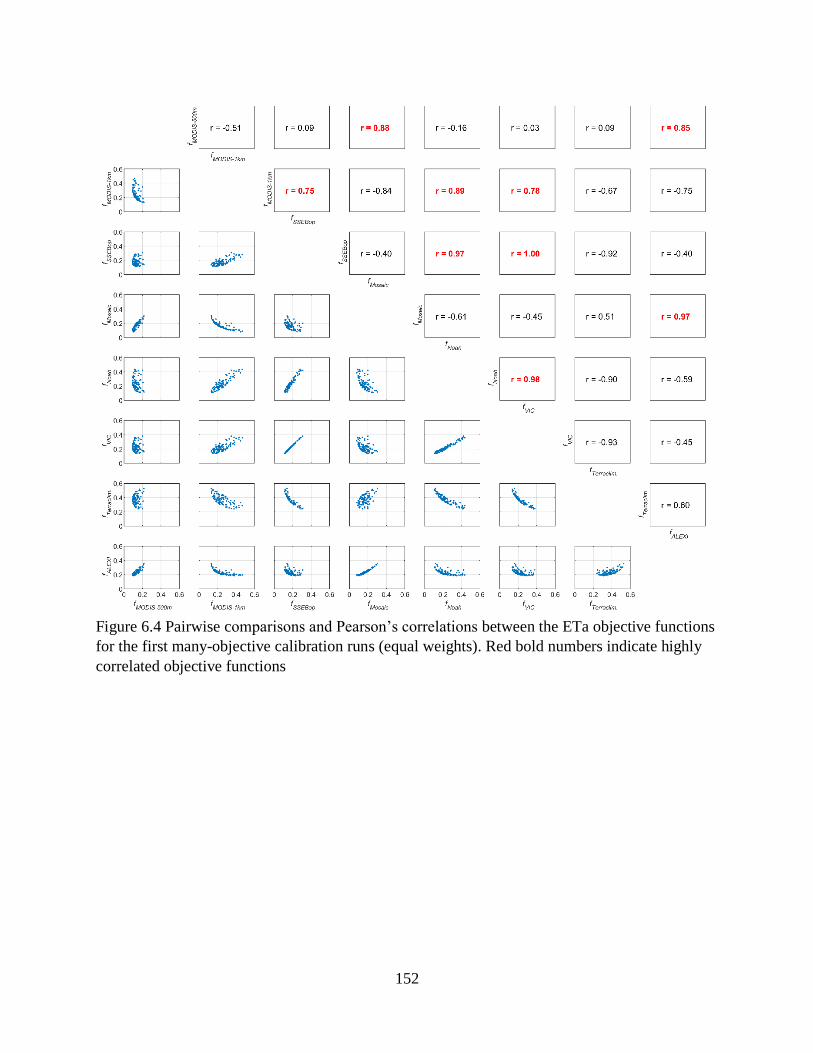
152

Figure 6.4 Pairwise comparisons and Pearson’s correlations between the ETa objective functions

for the first many-objective calibration runs (equal weights). Red bold numbers indicate highly

correlated objective functions

153

Figure 6.5. Pairwise comparisons and Pearson’s correlations between the ETa objective

functions for the second many-objective calibration runs (balanced weights). Red bold numbers

indicate highly correlated objective functions

Regarding the Pearson’s correlations among the ETa objective functions for both many-

objective calibrations, similar patterns were found. In fact, objectives functions found to be

highly correlated in the first run were also found to be highly correlated in the second run. This

can be explained since the calibration weights should not have had an impact on the magnitude

and pattern of the ETa products. Which is what the NSE objective function is a reflection of,

since the model calibration attempted to replicate the pattern and magnitude of each ETa

product. In fact, this furthers support the results found in the second study of this dissertation.

154

For example, Table 5.7 shows that there are similarities among the VIC, Noah, MOD16 1 km,

and SSEBop ETa products, which is mirrored in Figures 6.4 and 6.5. The results from Table 5.7

show that these datasets share similar magnitudes with watershed scale means of 39.56

mm/month for VIC, 42.03 mm/month for Noah, 45.39 mm/month for MOD16 1 km, and 39.05

mm/month for SSEBop. However, the result presented in Figures 6.4 and 6.5 not only confirm

that these products have similar magnitudes but also similar seasonal patterns. This is due to the

fact that the calibration process aims to match both the pattern and magnitude of each ETa

product and objective functions that are highly correlated show that as the model improved the

fit for one ETa product it also improved the fit for the other ETa products. This also explains

why the two MOD16 products are not highly correlated. While, these ETa products used the

same governing equations and thus seasonal pattern they have different magnitudes (watershed

scale means of 45.39 mm/month for the MOD16 1 km product and 54.98 mm/month for the

MOD16 500 m product), which is reflected by their lack of similarity in Table 5.7. Therefore,

when the calibration tried to replicate the MOD16 1 km dataset it pulled away from the values of

the MOD16 500m product. All of this shows that it is important to consider both the seasonal

pattern and the magnitude of the ETa products to improve hydrological model performance

through calibration.

Another use for the correlations presented in Figures 6.4 and 6.5 is to determine if the

calibration process contains redundant datasets and determine if a smaller set of ETa products

could be used form model calibration. For this the highly correlated datasets should be

considered. Correlation was determined by calculating Pearson’s correlations between all

objective functions, and the Pearson’s correlations for the ETa objective functions are presented

in the upper triangle of Figures 6.4 and 6.5. As can be seen, most of the objective functions have

155

low correlation values (r < 0.7). However, there were two groups of ETa products that were

highly correlated amongst each other; the first group includes the MOD16 1 km, SSEBop, Noah,

and VIC ETa products and the second group includes the MOD16 500 m, SSEBop, and Mosaic

products (Figures 6.3 and 6.5). The high correlations found among these products were also

echoed and noticeable in the pairwise regressions. The presence of these correlations indicates

that a smaller set of ETa products could be used for SWAT model calibration. However, in order

to determine which product to keep and which to remove, the ETa products with the highest

correlations to the streamflow objective function needed to be identified. The results of this show

that from the set of the MOD16 1 km, SSEBop, Noah, and VIC ETa products, the MOD16 1 km

product had the highest Pearson’s correlation with a value of 0.34; and from the set of MOD16

500 m, SSEBop, and Mosaic products, the MOD16 500 m product had the highest Pearson’s

correlation with a value of -0.09. Based on this, the SSEBop, Noah, and VIC products could be

removed while keeping the MOD16 1 km ETa product and the ALEXI and Mosaic products

could be removed while keeping the MOD16 500 m ETa product. Which if these removals were

done, the final ETa product set would include the MOD16 1 km, MOD16 500 m, and

TerraClimate ETa products. Future studies should explore the use of this simplified ETa product

set in hydrological model calibration.

6.3.3 Impact of Landuse Inputs on Remote Sensing Evapotranspiration Product Calibration

Performance

In order to examine the impacts of landuse on remotely sensed ETa products, a

comparison was performed between the MOD16 500 m and the SWAT model. The reasons for

this included that (1) not all ETa products utilize landuse files and (2) the MOD16 500 m

products had the best remote sensing ETa product performance in the multi-objective calibration

156

(Study 3) as well as the highest sensitivity to spatial and temporal variability (Study 2). In order

to perform this analysis, the USDA-NASS Cropland Data Layer was obtained for 2012, used in

the SWAT models developed in this dissertation, and the median landuse value of the MODIS

Land Cover Type 1 product for the period of study, used by the MOD16 500 m ETa product,

were obtained. Figure 6.3 shows a visual comparison between these two datasets, which in

general show a similar trend in the placement of landuse types (agricultural, forest, urban, and

wetland). However, due to the difference in resolution (30 m vs 500 m), the Cropland Data

Layer, is able to better capture the spatial variability across the landscape, especially regarding

urban and wetland areas. In order to better understand the difference among these datasets, Table

6.7 summarizes each dataset and displays the percentage of overlaps. As can be seen, from

Figure 6.3, the MOD16 Landuse characterizes the region as only having 1.3% urban and 0.4% as

wetland; which contrasts the 7.9% and 14.0% reported by the Cropland Data Layer for urban and

wetland, respectively. This also means that the MOD16 dataset classifies the region with more

agricultural and forest lands compared to the Cropland Data Layer. However, to determine the

overlap between the dataset the intersection of the two layers were performed. The fourth

column from the left in Table 6.7 reports the intersection value between the datasets in square

kilometers, which represents the regions of the Honeyoey watershed for which both datasets

agree on the landuse. These values were then divided by the respective areas for each landuse of

each dataset to calculate the percent of intersection. For example, when looking at agricultural

land, the intersection area was 603.3 km2, and for the Cropland Data Layer the total area of

agricultural land was 647.7 km2, by dividing the intersection by the total area the percentage of

intersection was found to be 93.1%. This means that 93.1% of the agricultural land reported by

the Cropland Data Layer was shared with the MOD16 product. This analysis was done for the

157

entire region as well as each major landuse using both datasets as reference. As can be seen when

looking at the entire region, 66.5% of the region was identified as being the same across both

landuse datasets. This shows that the majority of the region was the same for both datasets.

However, when looking at the individual landuses the lack of urban and wetland areas in the

MOD16 dataset plays a major role in the agreement among the two datasets. Since the areas for

both urban and wetland were small for the MOD16 dataset, only a small region of overlap was

identified (8.4 km2 and 0.9 km2, respectively). This translates to very small percentages of

intersection for the Cropland Data Layer (10.0% and 0.9%, respectively), since the overall areas

for those landuses was much higher (84.2 km2 and 148.6 km2, respectively). On the other hand,

the MOD16 dataset shows higher percentages of intersection for those landuses (59.9% and

23.9%, respectively), yet reported much smaller total areas for each landuses (14.1 km2 and 3.8

km2, respectively). In fact, this trend of the dataset with the smaller area for a specific landuse

reporting higher percentages of intersection and vice a versa held true for all landuses. Overall,

this shows that while the majority of the region is similar for both landuses datasets, there are

still a number of differences that indicate that the similarity among the ETa performances is

more likely linked to differences in governing equations and spatial resolutions than similarities

among the landuse datasets utilized.

158

Figure 6.6. Comparison of the landuse products utilized by (a) the SWAT and (b) the MOD16

500 m ETa product

159

Table 6.7. Comparison of the SWAT model and MOD16 500 m ETa product landuse datasets, CDL 2012 and MOD16, respectively

Land cover Area (km2) Regional Percentage (%) Percent of Intersection (%)

CDL 2012 MOD16 Intersection CDL 2012 MOD16 CDL 2012 MOD16

Agriculture 647.7 835.7 603.3 60.8 78.5 93.1 72.2

Urban 84.2 14.1 8.4 7.9 1.3 10.0 59.9

Forest 184.2 211.0 95.1 17.3 19.8 51.6 45.1

Wetland 148.6 3.8 0.9 14.0 0.4 0.6 23.9

Total 1064.6 1064.6 707.7 100.0 100.0 66.5 66.5

160

6.4 Conclusions

Throughout the course of this study, two different calibration techniques were explored,

1) multi-objective and 2) many-objective. In general, the best model performances were obtained

from the multi-objective calibrations. And considering all of the multi-objective calibrated

models, the model with the best streamflow performance was the Ensemble followed by Mosaic,

SSEBop, MOD16 500m, Noah, ALEXI, VIC, MOD16 1 km, and finally TerraClimate.

Meanwhile, when considering ETa performance, the SWAT model with the best performance

again utilized the Ensemble followed by the MOD16 500m, Mosaic, SSEBop, Noah, VIC,

MOD16 1km, ALEXI, and again finally TerraClimate. This shows that the Ensemble utilized in

this study had the best fit with the SWAT model and outperformed the individual ETa products.

Meanwhile, when considering the many-objective calibration, ETa performance was

found to be satisfactory; however, the streamflow performance was not satisfactory. This shows

that the many-objective calibration was not ideal for SWAT model calibration when considering

both streamflow and ETa simulation due to the fact that the search space is much larger than the

multi-objective approach. However, correlations among the ETa objective functions show that a

smaller set of ETa products should be explored in future studies, namely the MOD16 1 km,

MOD16 500 m, and TerraClimate ETa products. Another conclusion from the many-objective

calibration is the importance of both the magnitude and the seasonal pattern in model calibration.

However, it is important to note that this study was performed for only one watershed in

Michigan; therefore, future studies should expand this work to regions with different

physiographical and climatological zones. This would serve to confirm the robustness of the

techniques implemented this study. This would help improve our understanding of how each ETa

product performs in hydrological model calibration. Aligned with this is the fact that only the

161

SWAT model was used in this research, and different ETa products may fit better with different

hydrological models, therefore future studies should also explore the use of other widely used

hydrological models. Furthermore, other ensembling techniques should be performed to identify

the best for different regions.

6.5 Acknowledgment

Authors would like to thank Dr. Martha C. Anderson from USDA-ARS Hydrology and

Remote Sensing Laboratory at Beltsville, Maryland and Dr. Christopher R. Hain from NASA

Marshall Space Flight Center at Huntsville, AL for his help in providing ALEXI data. This work

is supported by the USDA National Institute of Food and Agriculture, Hatch project

MICL02359.

162

7. CONCLUSIONS

Throughout this dissertation, two main topics were explored, 1) the integration of

satellite-based remote sensing ETa products into the calibration and validation of hydrological

models and 2) the temporal and spatial performance of different satellite-based remotely sensed

ETa products. These two topics were examined in the Honeyoey watershed in the state of

Michigan, which is a region that lacks observed ETa data and is also considered as an area of

concern in the Great Lakes basin. In the first study, the introduction of satellite-based remote

sensing ETa products in hydrological model calibration was explored. In the second study, the

performance of different remote sensing ETa products was compared on both temporal and

spatial scales. And finally, in the third study, additional calibration techniques were expanded

building on the results of the first study. From these studies the major takeaways are as follows:

• Inclusion of ETa data in the model calibration process improved the overall model

performance. During the initial test of calibration techniques, the genetic algorithm

technique showed the greatest improvement of ETa simulation, but at the cost of

lowering the streamflow simulation. Meanwhile. the multi-variable technique was able to

improve ETa simulation and maintain/improve streamflow simulations. Thus, the use of

the multi-variable technique was further explored.

• Statistical analysis of the calibration results for the first study showed that even in cases

where calibration was satisfactory, there was still a significant difference between the

SWAT model outputs and the observed datasets at the 5% level of significance.

• Considering seasonal analysis among the ETa products, an overall pattern of less

variation in the spring and summer and more variation in the winter and fall was noticed.

However, there were no noticeable patterns found between seasons regarding similarities

163

among ETa products. This indicates that temporal variation is less influential when

compared to spatial variation.

• Considering seasonal analysis with individual ETa products, the majority (MOD16 500

m, MOD16 1 km, ALEXI, TerraClimate, SWAT, and the Ensemble) were able to

differentiate among all seasons. However, for ETa products from SSEBop, NLDAS-2:

Mosaic, NLDAS-2: Noah, and NLDAS-2: VIC similarity among the spring and fall

seasons were observed.

• Considering, spatial analysis of remotely sensed ETa products, two major clusters within

the ETa products were identified; datasets with higher ETa values reported by MOD16A2

500 m, NLDAS-2: Mosaic, TerraClimate, and ALEXI; and lower ETa values reported by

MOD16A2 1 km, SSEBop, NLDAS-2: Noah, NLDAS-2: VIC, and SWAT

• Among all of the ETa products tested, the MOD16A2 500 m product had the best spatial

performance, being able to distinguish between all of the major landuses for all seasons.

However, each products, except for ALEXI, were able to distinguish between the major

landuses for at least one season: MOD16A2 1 km: spring and summer; MOD16A2 500

m: winter, spring, summer, fall; SSEBop: winter; NLDAS-2 Mosaic: spring and summer;

NLDAS-2 Noah: winter and summer; NLDAS-2 VIC: spring; TerraClimate: spring;

ALEXI: none; SWAT: spring and summer; Ensemble: winter, summer, and fall.

• Considering the use of different calibration techniques, the multi-objective calibrations

resulted in better overall model performances than the many-objective calibration

technique.

• Considering the performance of individual ETa products in model calibration, all

products resulted in models that were satisfactorily calibrated for both streamflow and

164

ETa. However, use of the Ensemble in the multi-objective calibration resulted in a

SWAT model with the best performance compared to all other ETa products. Meanwhile

the introduction of the TerraClimate product resulted in the worst overall model

performance.

• Regarding the many-objective calibration technique, analysis of the Pareto frontier

showed that the calibration was successful for all ETa products; however, the calibration

was unable to achieve satisfactory results for streamflow performance. Results from the

spatial and temporal sensitivity and many-objective calibration showed that both the

magnitude and seasonal pattern of the ETa products play a major role in the agreement

among the ETa products and their performance in the many-objective calibration process.

This explained why the two MOD16 datasets that utilized the same technique were not

highly correlated during the many-objective calibration as well as their lack of agreement

in the spatial and temporal analysis.

• Based on both the temporal and spatial performances as well as the final multi-objective

calibration the MOD16 500 m ETa products has the best performance for the Honeyoey

watershed. After the MOD16 500 m, the ranking of the remaining remotely sensed ETa

products from best to worst is: MOD16 1 km, NLDAS-2: Mosaic, NLDAS-2: Noah,

SSEBop, NLDAS-2: VIC, ALEXI, and finally TerraClimate.

• Comparisons between the landuse datasets used for the SWAT model and the MOD16

500 m ETa products indicated that while the majority of the study area is similar between

both landuse datasets, the differences in ETa results is more likely originated from the

application of different governing equations and spatial resolutions of the individual ETa

products.

165

8. FUTURE RESEARCH RECOMMENDATIONS

This research explored the use of remote sensing ETa in hydrological model calibration

and the performance of remote sensing ETa products in a data scarce region. However, this is not

the definitive end for these knowledge gaps. Therefore, additional research should be performed

to address the limitations of this work. Possible areas for future research are presented below:

• Our study was performed for a small watershed in the state of Michigan. Therefore, the

recommended calibration techniques should also be examined in other regions with

different climatological and physiographical characteristics to improve our understanding

of the linkage of hydrological modeling and remote sensing data.

• Results from the first study indicated that while the model calibration was successful, it

was not able to replicate the ETa products. This indicates that there is still room to

improve the model calibration process to create even more realistic models that can

provide stakeholders, decision makers, and policy makers with more accurate results.

• Due to the lack of observed data, a simplified ensembling technique was utilized.

Therefore, in the future studies, it is recommended to examine the performance of

different ensembling techniques on capturing spatial and temporal variabilities of ETa

products.

• Identifying the best trade-off solution in the model calibration was done by giving

streamflow and ETa equal importance. However, experts’ inputs should be considered to

determine if this weighting assumption should be modified.

• Correlations among the ETa datasets, indicate that a smaller set of ETa products could be

used in the many-objective calibration process and should be explored in future studies.

166

• This dissertation explored the use of ETa data in hydrological model calibration, future

studies should explore the use of additional remotely sensed hydrological components

such as soil moisture.

167

APPENDIX

168

APPENDIX

Table S5.1. Average monthly ETa values for each dataset for agricultural lands with clusters indicated by superscripts for each column

Datasets Month


MOD16A2

1km

15.63a 20.94a 37.11a 37.62 54.89a 76.62a 98.07a 83.15a 42.37a 25.26a 20.41a 14.97a

MOD16A2

500m

16.29a 21.39a 37.69a 44.50a 70.02b 98.24b,c 126.96b 108.35 53.02b 26.39a,b 17.40b 10.95b

SSEBop 0.02 0.00 10.29b 26.16b 47.15a,c 87.57d 115.86b,c 99.60b 50.88b 10.96 5.73c 0.42c

NLDAS-

2:Mosaic

10.67b,c 11.39b,c 27.43c 61.21 97.41 121.73e 138.43 116.14 84.49 48.54c 22.03a 11.79b

NLDAS-

2:Noah

9.58b 12.02b 18.73d 28.52b 46.18c 78.30a 105.06d 101.68b 67.06c 27.73b 10.19 7.05d

NLDAS-

2:VIC

7.37 9.68c 10.08b 15.29 50.63a,c 93.34b,d 119.23b,c 96.95b 50.05b 16.29 5.78c 6.95c,d

TerraClimate —* —* 18.18b,c,d 81.94 101.76 110.83c,e 97.77a,d 86.81a,b,c 65.31b,c,d 49.58c 22.56a 1.39c,d

ALEXI 23.37 38.17 51.98 57.51 82.28 102.76c 123.09b 101.13b 66.95c 32.60d 19.75a 16.35a

SWAT 3.71 5.40 28.54c 42.24a 62.54 106.19c 102.18a,d 72.81c 48.28a,b 26.33a,b 16.87b,d 6.88d,e

Ensemble 11.74c 16.05 26.53c 44.09a 68.79b 96.17b 115.56c 99.23b 60.02d 29.67d 15.48d 9.34e


169

Table S5.2. Average monthly ETa values for each dataset for forest lands with clusters indicated by superscripts for each column

Datasets Month


MOD16A2

1km

16.47 22.63 37.46a 38.79a 67.33 95.23a 104.49a 84.17a 47.19a 25.36 19.66a 14.97a

MOD16A2

500m

14.95 20.47 37.17a 45.78b 90.59a,b 127.14 139.30b 116.29b 65.95b,c 27.10 16.56b 10.30b,c,d

SSEBop 0.02 0.01 10.02b 28.15c 54.26c 99.60a,b 122.22c 100.66c 54.51d 14.15a 5.75c 1.37e

NLDAS-

2:Mosaic

11.60a 13.03a 25.57c 53.95d 91.88a 116.00c 133.13b 116.03b 87.69 50.70b 21.65a,d 11.81b

NLDAS-

2:Noah

11.95a 14.22a 21.65d 29.56c 38.25d 64.11 94.43d 94.91d 67.71b 31.36c 12.05 8.35c,f

NLDAS-

2:VIC

8.14 9.92 10.57b 15.36 40.91d 77.83 108.71a 96.31c,d 49.27a 15.83a 6.51c 7.49c,f

TerraClimate —* —* 16.50b,c,d 81.41 101.45 110.58b,c 98.70a,d 88.50a,c,d 65.30b,c,d 49.22b 21.96a,d 1.20e

ALEXI 22.10 35.72 49.88 55.66d 85.29b 108.6c 125.04c 99.64c 67.11b 33.04c 19.12a 15.99a

SWAT 3.53 5.32 28.90e 40.11a 61.12c 84.92 68.43 65.47 65.84b,c 42.02 23.04d 8.65c,d,f

Ensemble 12.06a 16.40 26.21c,e 43.58b 71.25 99.89a,b,c 115.75 99.56c 63.09c 30.84c 15.41b 9.59d


170

Table S5.3. Average monthly ETa values for each dataset for urban lands with clusters indicated by superscripts for each column

Datasets Month


MOD16A2

1km

16.20a 22.44a 36.9a 37.69a 57.92a 74.93a 83.57 69.92 40.24a 25.04a 20.02a,b 15.29a

MOD16A2

500m

16.53a 22.12a 37.02a 44.60b 73.39b 96.76b 107.32a,b 92.38a 50.04b,c 26.06a 17.01a 10.57b

SSEBop 0.04 0.00 9.59b 24.94 48.12c 85.32c 105.52a,b 89.24a 46.65a,b,c 9.66 5.70c 0.01c

NLDAS-

2:Mosaic

10.14b,c 10.55b,c 28.53c 65.19 99.41d 124.34d 141.60 116.60 82.09d 47.06b 22.12b 11.71b

NLDAS-

2:Noah

8.64b 11.44b 17.9d 29.01 50.43a,c 84.32c 109.72a,b,c 105.00b 67.49e 26.50a 9.58 6.62d

NLDAS-

2:VIC

6.81 9.48c 9.65b 15.26 56.05a 101.77b,d 124.04 95.09a,b 49.26b,c 16.29 5.36c 6.54c,d

TerraClimate —* —* 20.02b,c,d 82.83 102.24d 110.26b,d 96.91a 86.54a 65.33b,d,e,f,g 50.14b 23.19a,b 1.70c,d

ALEXI 22.87 37.45 49.36 55.35 80.66 98.24b,d 115.04c 95.18a 63.36f 30.50a,c,d 18.53a,b 15.45a

SWAT 3.44 5.18 27.81c 40.74a 55.5a,c 72.35a 57.84 48.82 42.38a,c 31.51c 18.20a 7.19d,e

Ensemble 11.5c 16.03 26.19c 44.36b 71.03b 96.99b 110.46b 93.75a 58.06g 28.91d 15.19 9.04e


171

Table S5.4. Average monthly ETa values for each dataset for wetland lands with clusters indicated by superscripts for each column

Datasets Month


MOD16A2

1km

16.92 23.25 37.42a 38.21 66.47a 94.12a 103.31a 83.93a 45.87 25.34a 20.38a 15.77a

MOD16A2

500m

15.22 21.02 37.68a 45.59a,b 88.12b 123.71b 135.59b 113.85b 61.03a,b 26.61a,b 17.04 10.51b,c

SSEBop 0.04 0.06 11.24b 27.57c 54.16 99.80c,d 121.07c,d,e 101.85c 55.17c 13.86 5.94b 0.91d

NLDAS-

2:Mosaic

10.91a,b 12.10a 26.27c 57.00d 92.52 113.17c,e 128.98b,c 110.75b 83.71 49.82c 21.37a,c 11.62b

NLDAS-

2:Noah

10.24a 12.17a 17.28d 26.18c 42.43 74.71 102.39a 99.51a,c 66.06a,b 27.43b 9.91 7.20e

NLDAS-

2:VIC

7.84 9.90 10.11b 15.82 47.97 88.48f 117.67d,e 101.79c 53.98c 17.36 6.16b 7.39e

TerraClimate —* —* 19.00b,c,d 82.51 101.44 110.33b,c,d,e 96.77a 86.86a,c 64.95a,b,c 49.65c 22.99a,c 1.61d

ALEXI 22.73 36.62 49.93 55.87d 84.05b 106.14c,d,e 124.14b,c,d 99.60a,c 66.29a 32.18d 19.14a 15.93a

SWAT 4.05 5.95 32.01 47.95a 68.48a,c 90.46a,f 73.93 69.21 69.37a 42.51 23.53c 8.65c,e

Ensemble 11.87b 16.27 26.20c 43.59b 72.15c 101.31c,d 116.24e 99.77c 62.13b 30.28d 15.37 9.48c


172

Table S5.5. Average monthly ETa values for each dataset for alfalfa (ALFA) regions with clusters indicated by superscripts for each

column

Datasets Month


MOD16A2

1km 15.54a 20.90a 36.75a 39.18a 65.74 87.94 99.00a 80.57a 45.81a 24.95a 18.95a 14.23a

MOD16A2

500m 15.37a 20.69a 37.25a 46.42 86.85a,b 117.15a 131.25b,c 109.48b 61.80b,c 26.84b 16.47b 10.29b,c

SSEBop 0.02 0.01 8.33b 28.62b 54.69c 98.78b 121.28b 100.50c 55.05d 13.86c 5.54c 1.11d

NLDAS-

2:Mosaic 11.57b 12.87b 25.38c 52.79 90.39a 114.05a 131.68c 114.43b 86.39e 49.47d 21.43a 11.85b

NLDAS-

2:Noah 12.05b 14.37b 21.94d 29.52b 37.18 61.85 92.72d 93.47d 67.04b,c 31.39e 12.14 8.47c,e

NLDAS-

2:VIC 8.20 10.09 10.78e 15.42 41.24 78.09c 109.40e 96.95c,d 49.24a 15.82c 6.51c 7.45c,e

TerraClimate —* —* 16.02b,c,d,e 81.14 101.36 110.39a 98.84a,d,e 88.44a,c,d 65.53b,c,d 49.20d 21.55a,b 1.13d

ALEXI 22.26 35.97 50.13 56.55 85.60b 109.28a 124.86b,c 99.99c 67.65b 33.53e 18.97a 16.03a

SWAT 3.07 4.56 25.85c 38.03a 55.19c 73.62c 96.64a,d 92.51c,d 72.84b,c,e 29.44a,b,e 14.77d 5.39e

Ensemble 12.03b 16.24 25.93c 43.71 70.38 97.19b 113.63 97.98c,d 62.31c 30.63e 15.19d 9.47c


173

Table S5.6. Average monthly ETa values for each dataset for corn (CORN) regions with clusters indicated by superscripts for each

column

Datasets Month


MOD16A2

1km 15.58a 20.88a 37.24a 37.44 53.10a,b 74.38a 97.88a 83.92a 42.05a 25.28a 20.62a 15.04a

MOD16A2

500m 16.42a 21.45a 37.74a 44.17a 67.45c 95.16b,c 126.77b 109.36b 52.27b 26.30a,b 17.54b 11.01b

SSEBop 0.03 0.00 10.28b 25.78b 45.47a 84.79d 114.65b,c,d 99.63a,c 50.17b 10.42 5.72c 0.36c

NLDAS-

2:Mosaic 10.53b,c 11.05b,c 27.80c 62.77 98.60d 123.00e 139.33 116.08 83.83 48.08c 22.18a 11.82b

NLDAS-

2:Noah 9.17b 11.62b 18.29d 28.42b 47.66a,b 80.98a,d 107.08c 102.98b,c 66.97c 27.11b 9.89 6.83d

NLDAS-

2:VIC 7.27 9.65c 10.07b 15.28 52.48b 96.30b,c 120.98b,d 96.71a,c 49.97b 16.34 5.65c 6.87c,d

TerraClimate —* —* 18.34b,c,d 81.91 101.81d 110.91b,e 97.71a,c 86.55a,c 65.36b,c,d 49.61c 22.62a 1.39c,d

ALEXI 23.41 38.52 52.37 57.76 81.73 101.84b,c,e 122.91b 101.52c 67.00c 32.55d 19.84a 16.39a

SWAT 3.73 5.42 28.61c 42.65a 63.62c 115.34b,e 108.57c,d 71.70a 42.54a,b 25.83a,b 16.63b,d 6.92d,e

Ensemble 11.67c 15.99 26.61c 44.19a 68.54c 95.92c 115.91d 99.59c 59.70d 29.46d 15.51d 9.31e


174

Table S5.7. Average monthly ETa values for each dataset for field peas (FPEA) regions with clusters indicated by superscripts for

each column

Datasets Month


MOD16A2

1km 15.86a 21.59a 37.02a 38.28a 63.00a 90.61 97.33a 72.87a 43.22 25.34a 19.76a 14.84a

MOD16A2

500m 15.54a 21.91a 37.84a 45.85b 81.93b 114.36a 124.47b 95.57b,c 56.07a 27.25b 16.15b 10.22b,c

SSEBop 0.00 0.00 10.94b 27.72c 56.83a,c 104.65b 125.90b 102.54b 56.59a 15.50c 5.59c 0.94d

NLDAS-

2:Mosaic 11.60b 13.03b 25.74c 53.16d 86.80b 111.96a 128.81b 115.22 86.24 49.41d 21.47a 11.68b

NLDAS-

2:Noah 12.24b 14.16b 21.12d 29.87c 39.40d 65.75 95.74a 96.71c 69.07b 31.76e 12.24 8.48c,e

NLDAS-

2:VIC 8.12 9.76 10.38b 15.50 41.11d 78.43 108.40c 95.64b,c 49.54 15.98c 6.55c 7.71c,e

TerraClimate —* —* 19.68b,c,d 82.49 101.42 110.38a,b 98.14a,c 87.80a,b,c 64.78a,b,c 49.55d 22.89a 1.49d

ALEXI 23.09 36.70 50.07 56.59d 87.85b 109.90a,b 125.50b 101.39b,c 67.29b 32.52e 19.08a 15.91a

SWAT 3.70 5.50 28.43c 37.98a 54.03c 70.65 96.30a 76.34a 33.92 27.52a,b 15.96b 6.55e

Ensemble 12.24b 16.56 26.77c 43.68b 69.79 98.26 113.04 95.97b,c 61.60c 30.92e 15.47b 9.53c


175

Table S5.8. Average monthly ETa values for each dataset for deciduous forest (FRSD) regions with clusters indicated by superscripts

for each column

Datasets Month


MOD16A2

1km 16.47 22.63 37.46a 38.79a 67.33 95.22a 104.48a 84.16a 47.19a 25.36 19.67a 14.97a

MOD16A2

500m 14.95 20.47 37.17a 45.78b 90.59a,b 127.13b 139.29b 116.28b 65.94b,c 27.10 16.56b 10.3b,c,d

SSEBop 0.02 0.01 10.02b 28.15c 54.26c 99.60a,c 122.22c 100.66c 54.5d 14.15a 5.75c 1.37e

NLDAS-

2:Mosaic 11.60a 13.03a 25.57c 53.95d 91.88a 115.99d 133.13b 116.03b 87.69 50.70b 21.65a,d 11.81b

NLDAS-

2:Noah 11.95a 14.22a 21.64d 29.56c 38.25d 64.12 94.44d 94.91d 67.71b 31.36c 12.05 8.35c,f

NLDAS-

2:VIC 8.14 9.92 10.57b 15.36 40.91d 77.83 108.71a 96.31c,d 49.27a 15.83a 6.51c 7.49c,f

TerraClimate —* —* 16.50b,c,d 81.41 101.45 110.58b,c,d 98.70a,d 88.50a,c,d 65.30b,c,d 49.22b 21.96a,d 1.20e

ALEXI 22.10 35.72 49.88 55.66d 85.29b 108.6d 125.04c 99.65c 67.11b 33.04c 19.12a 15.99a

SWAT 3.53 5.32 28.90e 40.12a 61.12c 84.92 68.42 65.47 65.84b,c 42.02 23.04d 8.65c,d,f

Ensemble 12.06a 16.40 26.21c,e 43.58b 71.24 99.88a,c 115.75 99.56c 63.09c 30.84c 15.41b 9.59d


176

Table S5.9. Average monthly ETa values for each dataset for evergreen forest (FRSE) regions with clusters indicated by superscripts

for each column

Datasets Month


MOD16A2

1km 16.39a 23.34 36.79a 42.19a 84.70a 124.26a 128.12a 97.69a 55.75a,b,c 26.14 18.33a 14.14a

MOD16A2

500m 15.44a 21.85 35.09a 48.54 103.15b 156.60 160.06 130.24b 75.08d,e 28.85a 14.90b,c 10.06b,c,d

SSEBop 0.00 0.04 11.95b 28.91b 55.71c 101.13b,c 123.46a 104.63c 58.59a,b 15.38b 5.99d 2.79e

NLDAS-

2:Mosaic 11.61b 13.26a 25.64c,d 54.58c 96.89d 124.84a 144.84 125.07b 94.29 53.12c 22.05e 11.80b

NLDAS-

2:Noah 12.26b 15.17a,b 24.39c 32.34b 38.06e 60.88 92.32b 94.28a 69.22d,e,f 33.63d 13.10b 8.76c

NLDAS-

2:VIC 7.55 9.56 10.11b 15.04 39.70e 76.21 107.71c 94.12a 47.30c 15.21b 6.42d 7.03c

TerraClimate —* —* 17.32b,c,d 80.58 100.79b,d 110.41a,b,c 98.79b,c 88.50a 65.35a,b,d,e,f,g 48.83c 21.48a,e 1.09e

ALEXI 23.53 36.53 49.26 53.96c 84.18a 107.98b,c 123.90a 95.25a 65.64e,f,g 32.17a,d,e 18.32a,c 15.91a

SWAT 3.35 5.22 27.95c,d 36.22 59.88c 96.06b 72.68 64.08 45.68b,c 28.85a 16.07a,c 6.36c

Ensemble 12.28b 16.93b 26.55d 44.52a 75.40 107.79c 122.40a 103.72c 66.40f,g 31.67e 15.07c 9.62d


177

Table S5.10. Average monthly ETa values for each dataset for hay (HAY) regions with clusters indicated by superscripts for each

column

Datasets Month


MOD16A2

1km 16.87a 23.04a 37.52a 38.24a 67.22 95.36a 102.43a 83.90a 45.38 25.54a 21.15a 16.37a

MOD16A2

500m 16.31a 22.02a 37.34a 45.93b 82.61a 113.22b,c 127.15b,c 105.17b 55.53a,b 26.02a 17.15 10.37b,c

SSEBop 0.01 0.05 10.68b 27.35c 52.55b 95.37a,d 115.52d 98.06a,c 51.82a 11.54 5.77b 0.39d

NLDAS-

2:Mosaic 10.18b,c 10.33b 27.47c 55.38 87.34c 111.00b,c,e 132.52b 111.70d 78.95c 41.56b 20.22a 11.63b

NLDAS-

2:Noah 8.78b,c 10.41b 14.69d 23.99c 45.02 78.97f 104.95a 98.75a,b,c 63.19d 24.76a 8.64 6.44e,f

NLDAS-

2:VIC 7.22b 9.92b 10.13b 15.93 55.46b 99.97a,d,e,g 130.23b,c 108.20b,c,d 55.36a 17.98 5.81b 6.95d,e,f

TerraClimate —* —* 19.93b,c,d 82.84 102.31 110.16b,c,d,e,g 96.42a 86.50a,c 65.21a,b,c,d 49.87 23.19a 1.62d,e

ALEXI 24.24 39.32 53.37 59.79 84.36a,c 104.24c,d,e,g 123.50c 103.80b,c 67.76d 33.3 20.71a 16.81a

SWAT 3.70 5.60 28.37c 37.96a 54.45b 73.88f 69.19 64.10 56.22a,b 38.93b 20.64a 8.00c,e,f

Ensemble 11.83c 16.26 26.46c 43.68b 72.11 101.04d,e,g 116.59d 99.51c 60.40b 28.82 15.33 9.42b,c,f


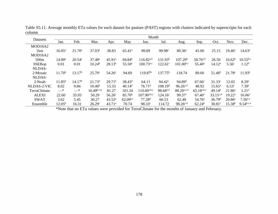
178

Table S5.11. Average monthly ETa values for each dataset for pasture (PAST) regions with clusters indicated by superscripts for each

column

Datasets Month


MOD16A2

1km 16.05a 21.70a 37.03a 38.83 65.41a 89.89 99.98a 80.36a 45.00 25.15 19.46a 14.63a

MOD16A2

500m 14.90a 20.54a 37.48a 45.91a 84.84b 116.82a,b 131.93b 107.29b 58.76a,b 26.50 16.62b 10.55b,c

SSEBop 0.01 0.01 10.24b 28.13b 55.50c 100.73a,c 122.61c 101.00b,c 55.40a 14.12a 5.56c 1.12d

NLDAS-

2:Mosaic 11.70b 13.17b 25.70c 54.26c 94.69 119.87b 137.75b 118.74 89.60 51.46b 21.78a 11.93b

NLDAS-

2:Noah 11.85b 14.17b 21.73d 29.71b 38.43d 64.11 94.42a 94.89d 67.66c 31.33c 12.02 8.29e

NLDAS-2:VIC 8.02 9.84 10.46b 15.33 40.14d 76.71d 108.19d 96.26c,d 48.92 15.65a 6.53c 7.39e

TerraClimate —* —* 16.49b,c,d 81.27 101.24 110.60a,b,c 98.68a,d 88.20a,c,d 65.18a,b,c 49.14b 21.86a 1.21d

ALEXI 22.60 35.93 50.29 56.26c 85.70b 107.90a,b,c 124.16c 99.37c 67.40c 33.15c,d 19.22a 16.06a

SWAT 3.62 5.45 30.27 43.52a 62.09a,c 77.28d 66.53 62.48 54.76a 36.79d 20.86a 7.50c,e

Ensemble 12.05b 16.31 26.29c 43.71a 70.74 98.33c 114.72 98.26c,d 62.24b 30.81c 15.38b 9.54b,c,e


179

Table S5.12. Average monthly ETa values for each dataset for sugar beet (SGBT) regions with clusters indicated by superscripts for

each column

Datasets Month


MOD16A2

1km 15.90 21.23a 38.44a 36.77 46.30a 65.78a 95.42a 83.65a 40.79 25.89a 22.18a 15.59a

MOD16A2

500m 18.58 23.20a 39.14a 42.29a 56.43a,b 82.03b 119.47b,c 102.12b,c,d 47.72a 26.58a 18.84b,c 11.48b

SSEBop 0.34 0.04 10.87b 25.38b 37.31 72.20a 108.52d 98.90b,c 48.34a 9.30 5.98d 0.08c

NLDAS-

2:Mosaic 9.94a 10.10b,c 28.29c 66.56 101.82c 126.91c 141.16 114.66d 81.01b 46.61b 22.26a,b 11.66b

NLDAS-

2:Noah 8.64a,b 11.30b 18.11d 29.56b 51.23a,b 85.5b 110.76b,d 106.04b,d 67.15c 26.49a 9.62 6.65d

NLDAS-

2:VIC 6.97b 9.69c 10.20b 15.22 58.12b 105.09d 125.03c 94.49a,b,c,d 49.51a 16.34 5.04d 6.55c,d

TerraClimate —* —* 19.09b,c,d 81.71 102.04c 111.65c,d 97.20a,d,e 85.19a,c 65.47b,c,d 49.76b 22.81a,b,c 1.51c,d

ALEXI 24.2 40.62 54.40 58.87 78.85 96.28e 121.32c 102.37b,c,d 67.45c 32.63c 20.23a,b,c 16.95a

SWAT 3.73 5.56 29.95c 45.13a 67.94d 96.74e 86.46e 79.03a 54.52a,d 30.62c,d 18.09c 6.85d

Ensemble 11.97 16.41 27.41c 44.54a 66.51d 93.18e 114.86b,c,d 98.43b,c 58.43d 29.20d 15.87 9.40


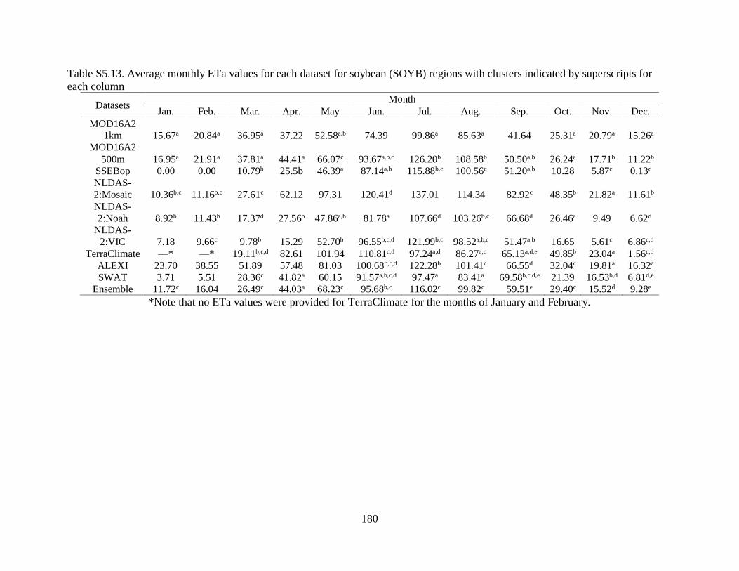
180

Table S5.13. Average monthly ETa values for each dataset for soybean (SOYB) regions with clusters indicated by superscripts for

each column

Datasets Month


MOD16A2

1km 15.67a 20.84a 36.95a 37.22 52.58a,b 74.39 99.86a 85.63a 41.64 25.31a 20.79a 15.26a

MOD16A2

500m 16.95a 21.91a 37.81a 44.41a 66.07c 93.67a,b,c 126.20b 108.58b 50.50a,b 26.24a 17.71b 11.22b

SSEBop 0.00 0.00 10.79b 25.5b 46.39a 87.14a,b 115.88b,c 100.56c 51.20a,b 10.28 5.87c 0.13c

NLDAS-

2:Mosaic 10.36b,c 11.16b,c 27.61c 62.12 97.31 120.41d 137.01 114.34 82.92c 48.35b 21.82a 11.61b

NLDAS-

2:Noah 8.92b 11.43b 17.37d 27.56b 47.86a,b 81.78a 107.66d 103.26b,c 66.68d 26.46a 9.49 6.62d

NLDAS-

2:VIC 7.18 9.66c 9.78b 15.29 52.70b 96.55b,c,d 121.99b,c 98.52a,b,c 51.47a,b 16.65 5.61c 6.86c,d

TerraClimate —* —* 19.11b,c,d 82.61 101.94 110.81c,d 97.24a,d 86.27a,c 65.13a,d,e 49.85b 23.04a 1.56c,d

ALEXI 23.70 38.55 51.89 57.48 81.03 100.68b,c,d 122.28b 101.41c 66.55d 32.04c 19.81a 16.32a

SWAT 3.71 5.51 28.36c 41.82a 60.15 91.57a,b,c,d 97.47a 83.41a 69.58b,c,d,e 21.39 16.53b,d 6.81d,e

Ensemble 11.72c 16.04 26.49c 44.03a 68.23c 95.68b,c 116.02c 99.82c 59.51e 29.40c 15.52d 9.28e


181

Table S5.14. Average monthly ETa values for each dataset for urban low-density (URLD) regions with clusters indicated by


Datasets Month


MOD16A2

1km 16.21a 22.76a 36.78a 38.13 58.52a 73.79 80.97a 67.57a 40.12 25.04a 19.83a 15.19a

MOD16A2

500m 16.61a 22.18a 36.66a 45.23a 74.21b 95.75a,b 104.37b,c 90.22b 49.74a 26.05a 16.76b 10.50b,c

SSEBop 0.03 0.00 9.25b 24.62 47.24c 83.60c 106.69b,c 89.65b,c 46.21a 9.49 5.32c 0.00d

NLDAS-

2:Mosaic 10.23b,c 10.78b,c 28.59c,d 64.08 97.66 122.43d 141.45 117.43 82.50 47.09b 21.94a,d 11.72a,b,c

NLDAS-

2:Noah 8.64b 11.49b 17.67e 28.52 49.79c 83.50c 109.00b,c 104.20d 67.50b,c 26.43a 9.51 6.58e

NLDAS-

2:VIC 6.74 9.39c 9.39b 15.30 54.90a 99.87a,b,d 123.68 95.91b,c,d 49.36a 16.33 5.54c 6.55d,e

TerraClimate —* —* 19.93b,c,d,e 82.88 102.35 110.28a,d 96.94b 86.72a,b,c 65.26a,b,c,d,e 50.15b 23.17a,d 1.71d,e

ALEXI 21.85 35.83 46.70 52.02 77.22b 95.48a,b,d 111.87c 93.05b,c 60.51b,d,e 28.39a,c 17.22b 14.56a,b

SWAT 3.56 5.30 29.05c 45.84a 66.81d 90.46b 77.07a 72.28a 66.22b,c,d 41.10 22.90d 8.18c,e,f

Ensemble 11.37c 15.88 25.68d 43.85a 70.23d 95.59a,b 109.37b,c 93.09c 57.65d,e 28.62c 14.91 8.90f


182

Table S5.15. Average monthly ETa values for each dataset for urban transportation (UTRN) regions with clusters indicated by


Datasets Month


MOD16A2

1km 16.18a 22.19a 36.99a 37.36a 57.46a 75.79 85.54a 71.71 40.33 25.04a 20.16a 15.38a

MOD16A2

500m 16.47a 22.08a 37.30a 44.12b 72.76b 97.53a,b 109.56b,c 94.02a,b,c 50.27a 26.08a 17.21 10.62b

SSEBop 0.04 0.00 9.85b 25.17 48.79c 86.63c 104.63b 88.93a,b 46.98a 9.78 5.99b 0.02c

NLDAS-

2:Mosaic 10.07b,c 10.37b,c 28.49c 66.04 100.74d 125.79d 141.71 115.98d 81.78b 47.03b 22.25a 11.71b

NLDAS-

2:Noah 8.64b 11.41b 18.08d 29.38 50.91c 84.95c 110.27b,c 105.60d 67.49c 26.55a 9.63 6.64d

NLDAS-

2:VIC 6.86 9.55c 9.84b 15.22 56.93a 103.21a,b,d 124.31d 94.47a,b,c,d 49.18a 16.27 5.22b 6.53c,d

TerraClimate —* —* 20.10b,c,d 82.80 102.16d 110.25a,d 96.89a,b 86.41a,b,c 65.39a,b,c,d 50.13b 23.20a 1.70c,d

ALEXI 23.64 38.68 51.38 57.88 83.27 100.33a,b,d 117.43d 96.80a,c 65.53c 32.10c 19.52a 16.13a

SWAT 3.34 5.09 26.87c 36.87a 46.94c 58.63 43.27 31.05 24.32 24.24a 14.65c 6.44d

Ensemble 11.60c 16.14 26.57c 44.75b 71.63b 98.06b 111.29c 94.24a,b,c 58.37d 29.12c 15.40c 9.15


183

Table S5.16. Average monthly ETa values for each dataset for woody wetlands (WETF) regions with clusters indicated by


Datasets Month


MOD16A2

1km 16.92 23.25 37.42a 38.21 66.47a 94.12a 103.31a 83.93a 45.87 25.34a 20.38a 15.77a

MOD16A2

500m 15.22 21.02 37.68a 45.59a,b 88.12b 123.71b 135.59b 113.85b 61.03a,b 26.61a,b 17.04 10.51b,c

SSEBop 0.04 0.06 11.24b 27.57c 54.16 99.80c,d 121.07c,d,e 101.85c 55.17c 13.86 5.94b 0.91d

NLDAS-

2:Mosaic 10.91a,b 12.10a 26.27c 57.00d 92.52 113.17c,e 128.98b,c 110.75b 83.71 49.82c 21.37a,c 11.62b

NLDAS-

2:Noah 10.24a 12.17a 17.28d 26.18c 42.43 74.71 102.39a 99.51a,c 66.06a,b 27.43b 9.91 7.20e

NLDAS-

2:VIC 7.84 9.90 10.11b 15.82 47.97 88.48f 117.67d,e 101.79c 53.98c 17.36 6.16b 7.39e

TerraClimate —* —* 19.00b,c,d 82.51 101.44 110.33b,c,d,e 96.77a 86.86a,c 64.95a,b,c 49.65c 22.99a,c 1.61d

ALEXI 22.73 36.62 49.93 55.87d 84.05b 106.14c,d,e 124.14b,c,d 99.60a,c 66.29a 32.18d 19.14a 15.93a

SWAT 4.05 5.95 32.01 47.95a 68.48a,c 90.46a,f 73.93 69.21 69.37a 42.51 23.53c 8.65c,e

Ensemble 11.87b 16.27 26.20c 43.59b 72.15c 101.31c,d 116.24e 99.77c 62.13b 30.28d 15.37 9.48c


184

Table S5.17. Average monthly ETa values for each dataset for winter wheat (WWHT) regions with clusters indicated by superscripts

for each column

Datasets Months


MOD16A2

1km 15.42a 20.72a 36.41a 37.83a 58.23a 80.27a 92.28a 74.20 41.66 25.23a 19.26a 14.34a

MOD16A2

500m 15.69a 21.01a 37.35a 45.03b 76.28 104.87b 121.46b,c 98.00a 53.81a,b 27.21b 16.88b 10.64b

SSEBop 0.02 0.00 10.53b 27.51c 50.91 93.23c 115.93b,c 94.20a,b 48.58a 12.23 5.80c 0.26c

NLDAS-

2:Mosaic 11.03b 12.21b 26.71c 57.31d 93.38 119.10d 137.87 119.03 87.49 49.58c 21.76a 11.65b

NLDAS-

2:Noah 10.85b 13.35b 20.74d 29.79c 42.59b 70.87 99.49d 98.37a,b 68.29c 30.37d 11.46 7.82d

NLDAS-

2:VIC 7.43 9.54 9.96b 15.21 45.93b 86.00a 114.75b,c 96.45a,b 49.25a,b 16.01 6.12c 7.09d

TerraClimate —* —* 17.82b,c,d 81.99 101.83 110.61b,d 97.82a,d 87.96a,b 65.25b,c,d 49.51c 22.35a 1.33c

ALEXI 23.95 37.88 51.36 57.09d 84.43 106.75b 124.53b 99.22a,b 66.17c 33.15d 19.89a 16.52a

SWAT 4.01 5.45 27.61c 39.83a 62.54a 108.06b 100.05d 58.82 30.89 26.96a,b 16.06b,d 6.72d

Ensemble 11.94b 16.21 26.45c 43.97b 69.20 96.46c 113.02c 95.93b 60.06d 30.41d 15.44d 9.32


185

Table S5.18. Average seasonal ETa values for each dataset for agricultural lands with clusters indicated by superscripts for each

column

Datasets Seasons


MOD16A2 1km 17.18a 43.21a 85.95 29.34a

MOD16A2 500m 16.21a 50.74 111.18a 32.27a,b,c

SSEBop 0.15b 27.87b 101.01b,c 22.52d

NLDAS-2:Mosaic 11.28c 62.02c 125.43 51.69e

NLDAS-2:Noah 9.55 31.15 95.01b 35.00b,c

NLDAS-2:VIC 8.00 25.33b 103.17c 24.04d

TerraClimate 1.08b 68.70c 98.47b,c 45.82e

ALEXI 25.96 63.92c 108.99a 39.77

SWAT 5.33 44.44a 93.72b,c 30.50a,b

Ensemble 12.37c 46.47a 103.65c 35.06c

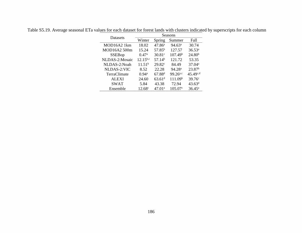
186

Table S5.19. Average seasonal ETa values for each dataset for forest lands with clusters indicated by superscripts for each column

Datasets Seasons


MOD16A2 1km 18.02 47.86a 94.63a 30.74

MOD16A2 500m 15.24 57.85b 127.57 36.53a

SSEBop 0.47a 30.81c 107.49b 24.80b

NLDAS-2:Mosaic 12.15b,c 57.14b 121.72 53.35

NLDAS-2:Noah 11.51b 29.82c 84.49 37.04a

NLDAS-2:VIC 8.52 22.28 94.28a 23.87b

TerraClimate 0.94a 67.88d 99.26a,c 45.49c,d

ALEXI 24.60 63.61d 111.09b 39.76c

SWAT 5.84 43.38 72.94 43.63d

Ensemble 12.68c 47.01a 105.07c 36.45a

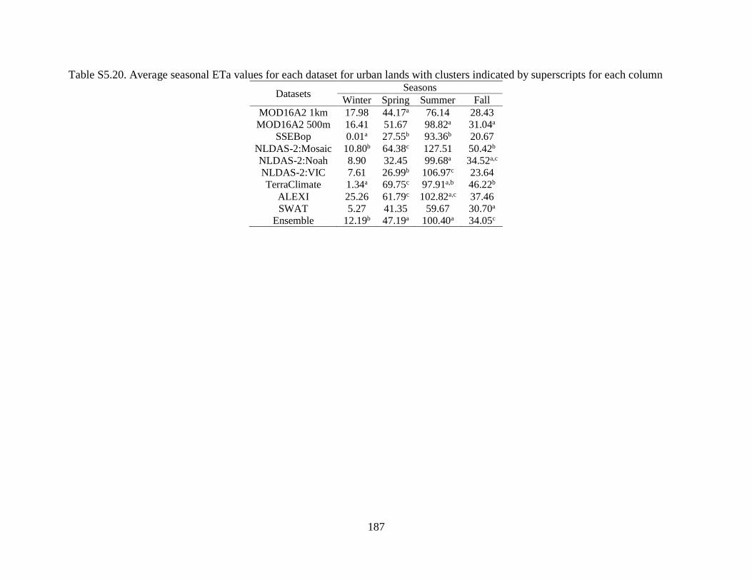
187

Table S5.20. Average seasonal ETa values for each dataset for urban lands with clusters indicated by superscripts for each column

Datasets Seasons


MOD16A2 1km 17.98 44.17a 76.14 28.43

MOD16A2 500m 16.41 51.67 98.82a 31.04a

SSEBop 0.01a 27.55b 93.36b 20.67

NLDAS-2:Mosaic 10.80b 64.38c 127.51 50.42b

NLDAS-2:Noah 8.90 32.45 99.68a 34.52a,c

NLDAS-2:VIC 7.61 26.99b 106.97c 23.64

TerraClimate 1.34a 69.75c 97.91a,b 46.22b

ALEXI 25.26 61.79c 102.82a,c 37.46

SWAT 5.27 41.35 59.67 30.70a

Ensemble 12.19b 47.19a 100.40a 34.05c

188

Table S5.21. Average seasonal ETa values for each dataset for wetland lands with clusters indicated by superscripts for each column

Datasets Seasons


MOD16A2 1km 18.65 47.37a 93.79a 30.53a

MOD16A2 500m 15.58 57.13b 124.38 34.89b

SSEBop 0.34a 30.99c 107.57b,c 24.99c

NLDAS-2:Mosaic 11.55b 58.60b,d 117.63 51.63d

NLDAS-2:Noah 9.87 28.63c 92.20a 34.47a,b

NLDAS-2:VIC 8.38 24.63 102.64a,b,d 25.84c

TerraClimate 1.26a 69.04d 97.99a,d 45.86d,e

ALEXI 25.09 63.29b,d 109.96c 39.20

SWAT 6.22 49.48a 77.87 45.13e

Ensemble 12.54b 47.31a 105.77b,c,d 35.93b

189

Table S5.22. Average seasonal ETa values for each dataset for alfalfa (ALFA) regions with clusters indicated by superscripts for each

column

Datasets Seasons


MOD16A2

1km 16.89 47.22a 89.17a,b 29.90

MOD16A2

500m 15.45 56.84b 119.29c 35.04a

SSEBop 0.38a 30.55c 106.85d 24.82b

NLDAS-

2:Mosaic 12.10b,c 56.19b 120.06c 52.43

NLDAS-

2:Noah 11.63b 29.55c 82.68a 36.85a

NLDAS-2:VIC 8.58 22.48 94.82e 23.86b

TerraClimate 0.89a 67.61d 99.22d,e,f 45.43c

ALEXI 24.75 64.09d 111.37 40.05c

SWAT 4.34 39.69 87.59b 39.01a,c

Ensemble 12.58c 46.67a 102.93f 36.05a

190

Table S5.23. Average seasonal ETa values for each dataset for corn (CORN) regions with clusters indicated by superscripts for each

column

Datasets Seasons


MOD16A2

1km 17.17a 42.59a 85.39 29.32a

MOD16A2

500m 16.29a 49.79 110.43a 32.04a,b,c

SSEBop 0.13b 27.17b 99.69b,c 22.10d

NLDAS-

2:Mosaic 11.13c 63.06c 126.14 51.36e

NLDAS-

2:Noah 9.21 31.46 97.01b 34.66b,c

NLDAS-2:VIC 7.93 25.94b 104.66a,b,c 23.99a,d

TerraClimate 1.08b 68.75c 98.39b,c 45.86e

ALEXI 26.11 63.95c 108.75a,c 39.80

SWAT 5.35 44.96a 98.54b,c 28.33a,b,d

Ensemble 12.32c 46.44a 103.81c 34.89c

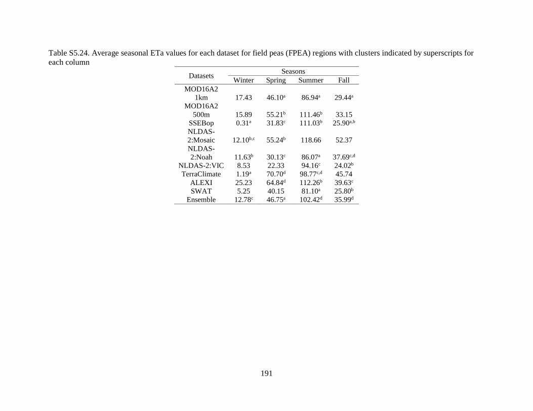
191

Table S5.24. Average seasonal ETa values for each dataset for field peas (FPEA) regions with clusters indicated by superscripts for

each column

Datasets Seasons


MOD16A2

1km 17.43 46.10a 86.94a 29.44a

MOD16A2

500m 15.89 55.21b 111.46b 33.15

SSEBop 0.31a 31.83c 111.03b 25.90a,b

NLDAS-

2:Mosaic 12.10b,c 55.24b 118.66 52.37

NLDAS-

2:Noah 11.63b 30.13c 86.07a 37.69c,d

NLDAS-2:VIC 8.53 22.33 94.16c 24.02b

TerraClimate 1.19a 70.70d 98.77c,d 45.74

ALEXI 25.23 64.84d 112.26b 39.63c

SWAT 5.25 40.15 81.10a 25.80b

Ensemble 12.78c 46.75a 102.42d 35.99d

192

Table S5.25. Average seasonal ETa values for each dataset for deciduous forest (FRSD) regions with clusters indicated by superscripts

for each column

Datasets Seasons


MOD16A2

1km 18.02 47.86a 94.62a 30.74

MOD16A2

500m 15.24 57.84b 127.57 36.53a

SSEBop 0.47a 30.81c 107.49b 24.80b

NLDAS-

2:Mosaic 12.15b,c 57.14b 121.72 53.35

NLDAS-

2:Noah 11.51b 29.82c 84.49 37.04a

NLDAS-2:VIC 8.52 22.28 94.28a 23.87b

TerraClimate 0.94a 67.88d 99.26a,c 45.49c,d

ALEXI 24.60 63.61d 111.10b 39.76c

SWAT 5.84 43.38 72.94 43.64d

Ensemble 12.68c 47.01a 105.07c 36.45a

193

Table S5.26. Average seasonal ETa values for each dataset for evergreen forest (FRSE) regions with clusters indicated by superscripts

for each column

Datasets Seasons


MOD16A2

1km 17.96 54.56 116.69 33.40a

MOD16A2

500m 15.78 62.26a 148.97 39.61b,c

SSEBop 0.94a 32.19b 109.74a 26.65d

NLDAS-

2:Mosaic 12.22b,c 59.03c 131.58 56.49

NLDAS-

2:Noah 12.06b 31.60b 82.49b 38.65b

NLDAS-2:VIC 8.05 21.62 92.68c 22.98

TerraClimate 0.85a 69.10a 99.23c 45.22c

ALEXI 25.32 62.47a,c 109.04a 38.71b

SWAT 4.98 41.35 77.61b 30.20a,d

Ensemble 12.94c 48.82 111.30a 37.71b

194

Table S5.27. Average seasonal ETa values for each dataset for hay (HAY) regions with clusters indicated by superscripts for each

column

Datasets Seasons


MOD16A2

1km 18.76 47.66a 93.90a 30.69a

MOD16A2

500m 16.23 55.29b 115.18b,c 32.90a

SSEBop 0.15a 30.19c 102.98d 23.04

NLDAS-

2:Mosaic 10.71 56.73b 118.41b 46.91b

NLDAS-

2:Noah 8.54b 27.90c,d 94.22a 32.20a

NLDAS-2:VIC 8.03b 27.17d 112.8b,c 26.38

TerraClimate 1.29a 69.74e 97.69a,d 46.09b,c

ALEXI 26.79 65.84e 110.51c 40.59b,c

SWAT 5.77 40.26 69.05 38.60c

Ensemble 12.50 47.42a 105.71 34.85

195

Table S5.28. Average seasonal ETa values for each dataset for pasture (PAST) regions with clusters indicated by superscripts for each

column

Datasets Seasons


MOD16A2

1km 17.46 47.09a 90.08a,b 29.87

MOD16A2

500m 15.33 56.08b 118.68 33.96

SSEBop 0.38a 31.29c 108.11c 25.03a

NLDAS-

2:Mosaic 12.26b,c 58.22b 125.45 54.28

NLDAS-

2:Noah 11.44b 29.96c 84.47a 37.00b

NLDAS-2:VIC 8.42 21.98 93.72a,b,d 23.70a

TerraClimate 0.95a 67.76d 99.16b,d 45.39c

ALEXI 24.87 64.08d 110.48c 39.92b,c

SWAT 5.53 45.30a 68.77 37.47b,c

Ensemble 12.63c 46.91a 103.77d 36.14b

196

Table S5.29. Average seasonal ETa values for each dataset for sugar beet (SGBT) regions with clusters indicated by superscripts for

each column

Datasets Seasons


MOD16A2

1km 17.58a 40.50 81.62a 29.62a

MOD16A2

500m 17.75a 45.95a 101.21b,c,d 31.05a

SSEBop 0.15b 24.52b 93.20a,b,e 21.21b

NLDAS-

2:Mosaic 10.57 65.56c 127.58 49.96c

NLDAS-

2:Noah 8.86 32.97 100.77b,c 34.42a,d

NLDAS-2:VIC 7.74 27.85b 108.20c,d,f 23.63b

TerraClimate 1.17b 69.00c 98.02b,c,e,f 46.01c,e

ALEXI 27.26 64.04c 106.65b,d,f 40.11e

SWAT 5.38 47.67a 87.41a,e 34.41d

Ensemble 12.59 46.16a 102.16b,c 34.50d

197

Table S5.30. Average seasonal ETa values for each dataset for soybean (SOYB) regions with clusters indicated by superscripts for

each column

Datasets Seasons


MOD16A2

1km 17.26a 42.25a,b 86.63a 29.25a

MOD16A2

500m 16.69a 49.43 109.49b 31.48b

SSEBop 0.04b 27.56c 101.19c 22.45c

NLDAS-

2:Mosaic 11.04c 62.35d 123.92 51.03d

NLDAS-

2:Noah 8.99 30.93 97.57d 34.21a,b,e

NLDAS-2:VIC 7.90 25.92c 105.69b,c 24.58c

TerraClimate 1.22b 69.28d 98.11c,d 46.01d

ALEXI 26.19 63.47d 108.13b 39.47f

SWAT 5.34 43.44a 90.82a,d 35.84a,b,e,f

Ensemble 12.35c 46.25b 103.84c 34.81e

198

Table S5.31. Average seasonal ETa values for each dataset for urban low-density (URLD) regions with clusters indicated by


Datasets Seasons


MOD16A2

1km 18.05 44.47a 74.11 28.33

MOD16A2

500m 16.43 52.03 96.78a,b 30.85a

SSEBop 0.01a 27.04b 93.31a 20.34

NLDAS-

2:Mosaic 10.91b 63.44c,d 127.10 50.51b

NLDAS-

2:Noah 8.90 31.99 98.90a,b 34.48a,c

NLDAS-2:VIC 7.56 26.53b 106.49c 23.74

TerraClimate 1.34a 69.77c 97.98a,b,c 46.19b,d

ALEXI 24.08 58.65d 100.13a,b 35.37c

SWAT 5.68 47.23a 79.94 43.40d

Ensemble 12.05b 46.59a 99.35b 33.73c

199

Table S5.32. Average seasonal ETa values for each dataset for urban transportation (UTRN) regions with clusters indicated by


Datasets Seasons


MOD16A2

1km 17.92 43.94a 77.68 28.51

MOD16A2

500m 16.39 51.39 100.37a 31.18a

SSEBop 0.02a 27.94b 93.40b 20.92b

NLDAS-

2:Mosaic 10.71b 65.09c 127.82 50.35c

NLDAS-

2:Noah 8.90 32.79 100.27a,c 34.56a,d

NLDAS-2:VIC 7.65 27.33b 107.33c 23.56e

TerraClimate 1.33a 69.73c 97.85a,b,c 46.24c

ALEXI 26.15 64.18c 104.85a,c 39.05

SWAT 4.95 36.90 44.31 21.07b,e

Ensemble 12.30b 47.65a 101.20a 34.30d

200

Table S5.33. Average seasonal ETa values for each dataset for woody wetlands (WETF) regions with clusters indicated by


Datasets Seasons


MOD16A2

1km 18.65 47.37a 93.79a 30.53a

MOD16A2

500m 15.58 57.13b 124.38 34.89b

SSEBop 0.34a 30.99c 107.57b,c 24.99c

NLDAS-

2:Mosaic 11.55b 58.60b,d 117.63 51.63d

NLDAS-

2:Noah 9.87 28.63c 92.20a 34.47a,b

NLDAS-2:VIC 8.38 24.63 102.64a,b,d 25.84c

TerraClimate 1.26a 69.04d 97.99a,d 45.86d,e

ALEXI 25.09 63.29b,d 109.96c 39.20

SWAT 6.22 49.48a 77.87 45.13e

Ensemble 12.54b 47.31a 105.77b,c,d 35.93b

201

Table S5.34. Average seasonal ETa values for each dataset for winter wheat (WWHT) regions with clusters indicated by superscripts

for each column

Datasets Seasons


MOD16A2

1km 16.83a 44.16a,b 82.25a 28.72

MOD16A2

500m 15.78a 52.89 108.11b 32.63

SSEBop 0.09b 29.65c 101.12c 22.20a

NLDAS-

2:Mosaic 11.63c,d 59.14d 125.33 52.94

NLDAS-

2:Noah 10.67c 31.04c 89.58a,c,d 36.71b

NLDAS-2:VIC 8.02 23.70 99.07c 23.79a

TerraClimate 1.04b 68.63e 98.80c,d 45.71c

ALEXI 26.12 64.29d,e 110.16b 39.74c

SWAT 5.39 43.33a 88.98a,d 24.63a

Ensemble 12.49d 46.54b 101.80c 35.30b

202

Table S5.35. Average seasonal values of the MOD16A2 500 m dataset for each major landuse category for each column

Landuse Season


Agriculture 16.21 50.74 111.18 32.27

Forest 15.24 57.85 127.57 36.53

Urban 16.41 51.67 98.82 31.04

Wetland 15.58 57.13 124.38 34.89

203

Table S5.36. Average seasonal values of the SSEBop dataset for each major landuse category for each column

Landuse Season


Agriculture 0.15 27.87a 101.01 22.52

Forest 0.47 30.81b 107.49a 24.80a

Urban 0.01 27.55a 93.36 20.67

Wetland 0.34 30.99b 107.57a 24.99a

204

Table S5.37. Average seasonal values of the NLDAS-2 Mosaic dataset for each major landuse category for each column

Landuse Season


Agriculture 11.28a 62.02 125.43 51.69a

Forest 12.15 57.14 121.72 53.35

Urban 10.80 64.38 127.51 50.42

Wetland 11.55a 58.60 117.63 51.63a

205

Table S5.38. Average seasonal values of the NLDAS-2 Noah dataset for each major landuse category for each column

Landuse Season


Agriculture 9.55 31.15a 95.01 35.00

Forest 11.51 29.82a,b 84.49 37.04

Urban 8.90 32.45 99.68 34.52a

Wetland 9.87 28.63b 92.20 34.47a

206

Table S5.39. Average seasonal values of the NLDAS-2 VIC dataset for each major landuse category for each column

Landuse Season


Agriculture 8.00 25.33 103.17a 24.04a

Forest 8.52a 22.28 94.28 23.87a,b

Urban 7.61 26.99 106.97 23.64a,b

Wetland 8.38a 24.63 102.64a 25.84

207

Table S5.40. Average seasonal values of the TerraClimate dataset for each major landuse category for each column

Landuse Season


Agriculture 1.08a 68.70 98.47 45.82a

Forest 0.94a 67.88 99.26 45.49

Urban 1.34a 69.75 97.91a 46.22

Wetland 1.26a 69.04 97.99a 45.86a

208

Table S5.41. Average seasonal values of the ALEXI dataset for each major landuse category for each column

Landuse Season


Agriculture 25.96 63.92a,b 108.99 39.77a

Forest 24.60a 63.61a,b 111.09a 39.76a

Urban 25.26a 61.79 102.82 37.46

Wetland 25.09a 63.29b 109.96a 39.20

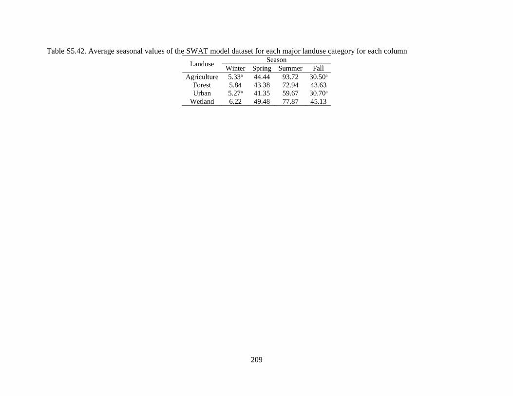
209

Table S5.42. Average seasonal values of the SWAT model dataset for each major landuse category for each column

Landuse Season


Agriculture 5.33a 44.44 93.72 30.50a

Forest 5.84 43.38 72.94 43.63

Urban 5.27a 41.35 59.67 30.70a

Wetland 6.22 49.48 77.87 45.13

210

Table S5.43. Average seasonal values of the Ensemble dataset for each major landuse category for each column

Landuse Season


Agriculture 12.37 46.47a 103.65 35.06

Forest 12.68 47.01a,b 105.07 36.45

Urban 12.19 47.19b 100.40 34.05

Wetland 12.54 47.31b 105.77 35.93

211

Table S5.44. Average monthly values of the MOD16A2 1km dataset for each major landuse category for each column

Landuse Month


Agriculture 15.63a 20.94 37.11a,b 37.62a 54.89 76.62a 98.07 83.15a,b 42.37 25.26a 20.41a 14.97a

Forest 16.47b 22.63a 37.46a 38.79 67.33 95.23 104.49 84.17a 47.19 25.36a 19.66b 14.97a

Urban 16.20a,b 22.44a 36.90b 37.69a 57.92 74.93a 83.57 69.92 40.24 25.04 20.02b,c 15.29a

Wetland 16.92 23.25 37.42a 38.21 66.47 94.12 103.31 83.93a,b 45.87 25.34a 20.38a,c 15.77

212

Table S5.45. Average monthly values of the MOD16A2 500 m dataset for each major landuse category for each column

Landuse Month


Agriculture 16.29 21.39 37.69a,b,c 44.50a 70.02 98.24a 126.96 108.35 53.02 26.39 17.4 10.95

Forest 14.95 20.47 37.17a,b,d 45.78b 90.59 127.14 139.30 116.29a 65.95 27.10 16.56 10.30a

Urban 16.53 22.12 37.02a,c,d 44.60a 73.39 96.76a 107.32 92.38 50.04 26.06 17.01a 10.57a,b

Wetland 15.22 21.02 37.68b,c,d 45.59b 88.12 123.71 135.59 113.85a 61.03 26.61 17.04a 10.51b

213

Table S5.46. Average monthly values of the SSEBop dataset for each major landuse category for each column

Landuse Month


Agriculture 0.02a,b,c 0.00 10.29a 26.16a 47.15a 87.57 115.86 99.60a 50.88 10.96 5.73a 0.42

Forest 0.02a 0.01 10.02a,b 28.15b 54.26b 99.60a 122.22a 100.66a,b 54.51a 14.15a 5.75a 1.37

Urban 0.04a,b,c 0.00 9.59a 24.94a 48.12a 85.32 105.52 89.24 46.65 9.66 5.70a 0.01

Wetland 0.04c 0.06 11.24b 27.57b 54.16b 99.80a 121.07a 101.85b 55.17a 13.86a 5.94a 0.91

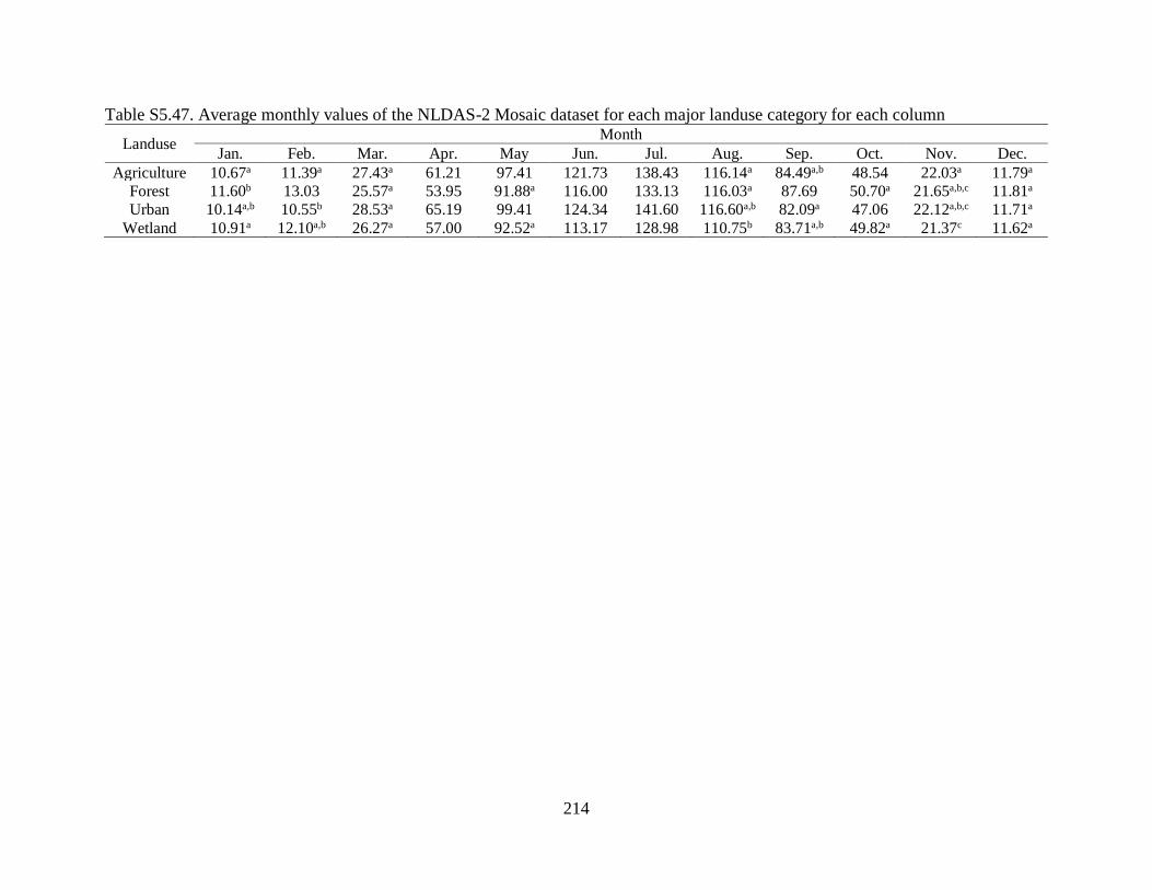
214

Table S5.47. Average monthly values of the NLDAS-2 Mosaic dataset for each major landuse category for each column

Landuse Month


Agriculture 10.67a 11.39a 27.43a 61.21 97.41 121.73 138.43 116.14a 84.49a,b 48.54 22.03a 11.79a

Forest 11.60b 13.03 25.57a 53.95 91.88a 116.00 133.13 116.03a 87.69 50.70a 21.65a,b,c 11.81a

Urban 10.14a,b 10.55b 28.53a 65.19 99.41 124.34 141.60 116.60a,b 82.09a 47.06 22.12a,b,c 11.71a

Wetland 10.91a 12.10a,b 26.27a 57.00 92.52a 113.17 128.98 110.75b 83.71a,b 49.82a 21.37c 11.62a

215

Table S5.48. Average monthly values of the NLDAS-2 Noah dataset for each major landuse category for each column

Landuse Month


Agriculture 9.58 12.02a 18.73 28.52 46.18 78.30 105.06 101.68 67.06a 27.73 10.19 7.05a

Forest 11.95 14.22 21.65 29.56a 38.25 64.11 94.43 94.91 67.71a 31.36 12.05 8.35

Urban 8.64 11.44 17.90 29.01a 50.43 84.32 109.72 105.00 67.49a 26.50 9.58a 6.62

Wetland 10.24 12.17a 17.28 26.18 42.43 74.71 102.39 99.51 66.06 27.43 9.91a 7.20a

216

Table S5.49. Average monthly values of the NLDAS-2 VIC dataset for each major landuse category for each column

Landuse Month


Agriculture 7.37 9.68a 10.08a 15.29a 50.63 93.34 119.23a 96.95a 50.05a 16.29a 5.78 6.95a

Forest 8.14a 9.92a 10.57a 15.36a 40.91 77.83 108.71 96.31a 49.27a 15.83a 6.51a 7.49a,b

Urban 6.81 9.48a 9.65b 15.26a 56.05 101.77 124.04 95.09a,b 49.26a 16.29a,b 5.36 6.54a

Wetland 7.84a 9.90a 10.11a,b 15.82 47.97 88.48 117.67a 101.79b 53.98 17.36b 6.16a 7.39b

217

Table S5.50. Average monthly values of the TerraClimate dataset for each major landuse category for each column

Landuse Month


Agriculture —* —* 18.18 81.94a 101.76a 110.83a 97.77 86.81a 65.31a 49.58a 22.56 1.39a

Forest —* —* 16.50 81.41a,b 101.45a,b,c 110.58a,b 98.70 88.50 65.30a,b 49.22 21.96 1.20a

Urban —* —* 20.02 82.83a,b 102.24b 110.26b 96.91b 86.54a,b 65.33a,b 50.14 23.19 1.70a

Wetland —* —* 19.00 82.51b 101.44c 110.33b 96.77b 86.86a,b 64.95b 49.65a 22.99 1.61a


218

Table S5.51. Average monthly values of the ALEXI dataset for each major landuse category for each column

Landuse Month


Agriculture 23.37a 38.17a 51.98 57.51 82.28 102.76 123.09a 101.13a 66.95a,b 32.60a,b 19.75 16.35a

Forest 22.10a 35.72 49.88a 55.66a 85.29a 108.60a 125.04a 99.64a,b 67.11a 33.04a 19.12a 15.99a,b,c

Urban 22.87a 37.45a,b 49.36a 55.35a 80.66 98.24 115.04 95.18 63.36 30.50 18.53a 15.45b

Wetland 22.73a 36.62b 49.93a 55.87a 84.05a 106.14a 124.14a 99.60b 66.29b 32.18b 19.14a 15.93b,c

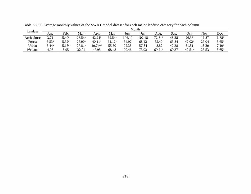
219

Table S5.52. Average monthly values of the SWAT model dataset for each major landuse category for each column

Landuse Month


Agriculture 3.71 5.40a 28.54a 42.24a 62.54a 106.19 102.18 72.81a 48.28 26.33 16.87 6.88a

Forest 3.53a 5.32a 28.90a 40.11b 61.12a 84.92 68.43 65.47 65.84 42.02a 23.04 8.65b

Urban 3.44a 5.18a 27.81a 40.74a,b 55.50 72.35 57.84 48.82 42.38 31.51 18.20 7.19a

Wetland 4.05 5.95 32.01 47.95 68.48 90.46 73.93 69.21a 69.37 42.51a 23.53 8.65b

220

Table S5.53. Average monthly values of the Ensemble dataset for each major landuse category for each column

Landuse Month


Agriculture 11.74a 16.05a 26.53a 44.09a 68.79 96.17a 115.56a 99.23a 60.02 29.67 15.48a 9.34a

Forest 12.06b 16.40a,b 26.21a,b 43.58b 71.25a 99.89 115.75a 99.56a 63.09 30.84 15.41a,b 9.59a

Urban 11.50 16.03a,b 26.19a,b 44.36a 71.03a 96.99a 110.46 93.75 58.06 28.91 15.19b 9.04

Wetland 11.87a,b 16.27b 26.20b 43.59b 72.15 101.31 116.24a 99.77a 62.13 30.28 15.37a,b 9.48a

221

Table S5.54. Average monthly values of the MOD16A2 1km dataset for each individual landuse with clusters indicated by


Landuse Month


ALFA 15.54a 20.9a 36.75a,b,c 39.18a 65.74a,b 87.94a 99.00a,b 80.57a 45.81a 24.95a,b,c,d 18.95a 14.23a,b

CORN 15.58a,b 20.88a,b 37.24a,b,d 37.44b,c,d 53.10 74.38b,c 97.88a 83.92b,c 42.05b 25.28a,b,c,e,f 20.62b 15.04c,d,e,f

FPEA 15.86a,b,c 21.59a,b,c 37.02a,b,c,d 38.28b,e 63.00 90.61a,d 97.33a,b,c 72.87d,e 43.22b,c,d 25.34a,b,c,d,e,f,g 19.76c,d,e,f 14.84c,d,e,f,g

FRSD 16.47c,d,e 22.63c,d,e 37.46a,c,d 38.79a 67.33c 95.22e 104.48d 84.16b,c,f 47.19 25.36a,d,e,f,g 19.67c,d 14.97c,d,e,g

FRSE 16.39a,b,c,d,e 23.34c,d,f 36.79a,b,c,d 42.19 84.70 124.26 128.12 97.69 55.75 26.14g,h 18.33 14.14a,b,c,f,g

HAY 16.87d,e 23.04d,e,f 37.52a,c,d 38.24a,b,e 67.22a,c 95.36e,f 102.43b,d,e 83.90b,c,f 45.38a,c 25.54b,e,f,g,h 21.15g 16.37

PAST 16.05a,b,c 21.7b,c 37.03a,b,c 38.83a 65.41b 89.89d 99.98a,b 80.36a 45.00c 25.15a,b,c,d,e 19.46e 14.63a,c,d,f,g

SGBT 15.90a,b,c,d,e 21.23a,b,c,e 38.44d 36.77b,c,f 46.30 65.78 95.42a,b,c 83.65a,b,c,f 40.79b,d 25.89f,g,h 22.18 15.59d,e,f,g,h

SOYB 15.67a,b 20.84a,b 36.95b,c,d 37.22c,f 52.58 74.39b,c 99.86a,b 85.63b,f 41.64b,d 25.31a,b,c,e,f,h 20.79g 15.26d,e,f,g,h

URLD 16.21a,b,c,d 22.76d,e,f 36.78a,b,c 38.13b,e 58.52d 73.79b 80.97 67.57 40.12d 25.04a,b,c,d 19.83c,d 15.19c,d,e,f,g

UTRN 16.18b,c,d 22.19b,c,e,f 36.99a,b,c,d 37.36c,d,f 57.46e 75.79c 85.54 71.71d 40.33d 25.04b,c,d,f 20.16f 15.38c,d,e,g,h

WETF 16.92e 23.25d,f 37.42a,c,d 38.21e 66.47a,b,c 94.12f 103.31e 83.93b,c,f 45.87a 25.34a,b,e,f 20.38b,f 15.77g,h

WWHT 15.42a 20.72a 36.41b 37.83b,d,e,f 58.23d,e 80.27 92.28c 74.20e 41.66b,d 25.23a,b,c,d,e,f 19.26a,d,e 14.34a,b,f

222

Table S5.55. Average monthly values of the MOD16A2 500 m dataset for each individual landuse with clusters indicated by


Landuse Month

Jan. Feb. Mar. Apr. May Jun. Jul. Aug. Sep. Oct. Nov. Dec. ALFA 15.37a,b 20.69a 37.25a,b,c,d,e 46.42a 86.85a 117.15a 131.25a,b 109.48a,b 61.80a 26.84a,b 16.47a 10.29a,b

CORN 16.42c,d 21.45b 37.74a,b,c 44.17b 67.45 95.16b,c 126.77a 109.36a,b,c 52.27b,c 26.30c,d,e 17.54 11.01

FPEA 15.54a,b,e 21.91b,c 37.84a,b,c,d,e,f 45.85a,c,d 81.93a,b,c 114.36a,d 124.47a,b,c 95.57d,e,f,g 56.07b,c,d,e 27.25a,b,c,d,e,f 16.15 10.22a,b,c

FRSD 14.95f 20.47d 37.17a,b,d,e 45.78a,c,d 90.59 127.13 139.29 116.28h 65.94 27.10a 16.56a,b 10.30a,b

FRSE 15.44a,b,e,f 21.85b,c 35.09d 48.54 103.15 156.60 160.06 130.24 75.08 28.85f 14.90 10.06a,b,c

HAY 16.31c 22.02c 37.34a,b,c,d,e 45.93a,c,e 82.61b 113.22d 127.15a,b,c 105.17a,b,c,d 55.53b,d 26.02c 17.15c,d,e 10.37a,b,c,d

PAST 14.90f 20.54a,d 37.48a,b,c,e 45.91a,c,d 84.84c 116.82a,d 131.93b 107.29a,c 58.76e 26.50b,d,e 16.62a,b 10.55c,d

SGBT 18.58 23.20 39.14f 42.29 56.43 82.03 119.47c 102.12d,e 47.72f 26.58a,b,c,d,e 18.84 11.48e

SOYB 16.95 21.91c 37.81a,b,c,e 44.41b,e 66.07 93.67b 126.20a 108.58a,b,c 50.50g 26.24b,c,d,e 17.71 11.22e

URLD 16.61d 22.18c 36.66a,d 45.23c,d,e 74.21 95.75b,c 104.37 90.22f 49.74f,g 26.05c,d,e 16.76a,b,c,d 10.50a,b,c,d

UTRN 16.47c,d 22.08c 37.30a,c,e 44.12b 72.76 97.53c 109.56 94.02g 50.27g 26.08c,d 17.21c,e 10.62a,b,c,d

WETF 15.22a,b 21.02e 37.68b,c,e 45.59a,c,d 88.12a 123.71 135.59 113.85h 61.03a 26.61a,b,e 17.04b,c,e 10.51b,c,d

WWHT 15.69b,e 21.01e 37.35a,b,c,d,e 45.03a,b,d,e 76.28 104.87 121.46a,c 98.00d,e 53.81b,c,d 27.21a,b 16.88b,d,e 10.64c,d

223

Table S5.56. Average monthly values of the SSEBop dataset for each individual landuse with clusters indicated by superscripts for

each column

Landuse Month

Jan. Feb. Mar. Apr. May Jun. Jul. Aug. Sep. Oct. Nov. Dec. ALFA 0.02a,b 0.01a,b,c,d,e 8.33a,b 28.62a 54.69a,b 98.78a 121.28a 100.50a,b,c 55.05a,b 13.86a,b 5.54a,b,c,d 1.11a

CORN 0.03a,b 0.00a,b,c,d,e 10.28a,c,d,e,f 25.78b 45.47c 84.79b,c 114.65b 99.63a,b 50.17c,d,e 10.42c,d,e 5.72a,b,c,d 0.36b

FPEA 0.00c 0.00a,b,c 10.94a,c,d,e,f 27.72a,b 56.83a 104.65d 125.90c 102.54a,c,d 56.59a,b,f 15.50a 5.59a,b,c,d 0.94c

FRSD 0.02a 0.01a 10.02a,c,d,e 28.15a 54.26b 99.60a 122.22a,c 100.66a,b,c 54.50a 14.15a,b 5.75a,b,c 1.37

FRSE 0.00d 0.04a,b,c,d,e,f 11.95a,c,d,f 28.91a 55.71a,b 101.13a,d,e 123.46a,c 104.63c,d 58.59f 15.38a,b 5.99a,b,c,d 2.79

HAY 0.01a,b,c,d,e 0.05a,b,c,d,e,f 10.68a,c,d,e,f 27.35a,b 52.55a,b,d 95.37f 115.52b,d 98.06a,b 51.82c,d 11.54c,d,f 5.77a,b,c,d 0.39b,d

PAST 0.01a 0.01a,b,c,d,e 10.24a,c,d,e 28.13a 55.50a,b 100.73e 122.61a,c 101.00a,b,c 55.40b 14.12a,b 5.56a,b,d 1.12a

SGBT 0.34 0.04a,b,c,d,e,f 10.87a,c,d,e,f 25.38a,b 37.31 72.20 108.52e 98.90a,b,c 48.34c,e 9.30c,e,f 5.98a,b,c,d 0.08d,e,f

SOYB 0.00e 0.00a,b,d,e 10.79c,e,f 25.5b 46.39c 87.14b 115.88d 100.56a,b 51.20d 10.28c,d,e,f 5.87a,b,c,d 0.13e

URLD 0.03a,b 0.00a,c,d 9.25a,b,d,e,f 24.62b 47.24c 83.60c 106.69e,f 89.65e 46.21e 9.49d,e,f 5.32a,c,d 0.00f

UTRN 0.04a,b 0.00a,c,e 9.85b,c,d,e,f 25.17b 48.79 86.63b,c 104.63f 88.93e 46.98e 9.78d,e,f 5.99b,c,d 0.02f

WETF 0.04b 0.06f 11.24c,d,e,f 27.57a 54.16a,b 99.80a,e 121.07a,c 101.85c,d 55.17a,b 13.86b 5.94a,b,c,d 0.91c

WWHT 0.02a,e 0.00b,c,d,e 10.53a,c,d,e 27.51a 50.91d 93.23f 115.93b,d 94.20 48.58e 12.23c 5.80a,b,c,d 0.26b,d

224

Table S5.57. Average monthly values of the NLDAS-2 Mosaic dataset for each individual landuse with clusters indicated by


Landuse Month

Jan. Feb. Mar. Apr. May Jun. Jul. Aug. Sep. Oct. Nov. Dec. ALFA 11.57a,b 12.87a,b,c 25.38a,b 52.79a 90.39 114.05a 131.68a 114.43a,b,c,d,e,f 86.39a,b,c 49.47a 21.43a 11.85a,b,c,d

CORN 10.53c,d,e,f 11.05d 27.8a,b,c,d,e 62.77 98.60a 123.00b 139.33b 116.08a,b,c,d,e,g 83.83a,b,d 48.08b 22.18b,c,d 11.82a,b,c

FPEA 11.60a,b,g 13.03a,b,e 25.74a,b,c 53.16a 86.80b 111.96a,c 128.81c 115.22a,b,c,d,f 86.24a,b,c 49.41a,b 21.47a,b 11.68a,b,d

FRSD 11.60a,b 13.03a,b,e 25.57a,c 53.95b 91.88c 115.99 133.13d 116.03a,b,c,f 87.69c 50.70c 21.65a,b,c 11.81a,b,d

FRSE 11.61a,b,c,d,e,g,h 13.26a,e 25.64a,b,c,d,e 54.58c 96.89a,d 124.84b,d,e 144.84b,e,f 125.07 94.29 53.12 22.05c,d 11.80a,b,d

HAY 10.18c,d,f,h,i 10.33f,g 27.47d,e 55.38a,b,c,d 87.34b 111.00c 132.52a,d 111.70a,b,d,e,f 78.95e,f,g 41.56 20.22 11.63a,b,c,d

PAST 11.70a,g 13.17e 25.7a,c,d,e 54.26c 94.69 119.87b,f 137.75b,e,g 118.74a,b,f,g 89.60 51.46 21.78a,b,c,d 11.93a,c,d

SGBT 9.94e,f,h,i 10.10f 28.29a,b,c,d,e 66.56 101.82 126.91d 141.16b,f 114.66a,c,d,e,f,g 81.01d,e,f 46.61 22.26a,b,c,d 11.66a,b,c,d

SOYB 10.36c,f,h,i 11.16h 27.61a,b,c,d,e 62.12 97.31d 120.41f 137.01g 114.34a,b,c,d,e,f,g 82.92d,g 48.35a,b 21.82a,b,d 11.61b,c,d

URLD 10.23b,c,d,e,f,i 10.78d,h,i 28.59d 64.08 97.66d 122.43b,f 141.45b,e,f 117.43b,c,d,e,g 82.50d,g 47.09d 21.94a,b,d 11.72a,b,c,d

UTRN 10.07c,d,e,f,i 10.37g 28.49a,b,c,d,e 66.04 100.74 125.79e 141.71e,f 115.98b,c,d,e,f,g 81.78d,e,g 47.03d 22.25a,b,c,d 11.71a,b,c,d

WETF 10.91c,d,e,f,h,i 12.10c,i 26.27a,b,c,e 57.00d 92.52c,e 113.17a,c 128.98c 110.75a,b,e,f 83.71a,d,f,g 49.82a,c 21.37a,b,d 11.62a,b,d

WWHT 11.03c,d,e,h 12.21b,c,i 26.71d,e 57.31d 93.38e 119.1f 137.87b,g 119.03a,b,g 87.49b,c 49.58a 21.76a,b,d 11.65a,b,c,d

225

Table S5.58. Average monthly values of the NLDAS-2 Noah dataset for each individual landuse with clusters indicated by


Landuse Month


ALFA 12.05a 14.37a 21.94a 29.52a,b,c,d 37.18 61.85a 92.72a 93.47 67.04a,b,c,d 31.39a 12.14a 8.47a,b

CORN 9.17b 11.62b,c 18.29b 28.42a 47.66a 80.98 107.08 102.98a 66.97a,b,c,d,e 27.11b 9.89b 6.83c,d,e

FPEA 12.24a,c,d 14.16a,d 21.12c,d 29.87b,c,e 39.40b 65.75 95.74 96.71b 69.07a,f 31.76 12.24a,c 8.48a,b,f

FRSD 11.95c 14.22d 21.64c 29.56a,b,c,d 38.25c 64.12b 94.44b 94.91c 67.71a,b,c,e,g 31.36a 12.05a,c 8.35a

FRSE 12.26a 15.17 24.39 32.34 38.06b,c,d 60.88a 92.32a 94.28c 69.22a,f,g 33.63 13.10 8.76b

HAY 8.78b,e,f 10.41 14.69 23.99 45.02 78.97 104.95 98.75b,d,e 63.19 24.76 8.64 6.44c,d,g

PAST 11.85d 14.17d 21.73a 29.71b,c,e 38.43d 64.11b 94.42b 94.89c 67.66a,b,c,e 31.33a 12.02c 8.29f

SGBT 8.64e 11.30e,f 18.11b 29.56b,d,e 51.23 85.50 110.76 106.04 67.15b,c,d,e,f,g 26.49c 9.62b,d,e 6.65c,d,e,g

SOYB 8.92f 11.43b,e,f 17.37e 27.56 47.86a 81.78 107.66 103.26a 66.68b,c,d,e 26.46c 9.49d,e 6.62c,g

URLD 8.64e 11.49b,c,e,f 17.67f 28.52a,d 49.79 83.50 109.00 104.20 67.50a,b,d,e,f,g 26.43c 9.51d 6.58c,g

UTRN 8.64e 11.41b,c,f 18.08b 29.38c,d,e 50.91 84.95 110.27 105.60 67.49a,b,d,e,f,g 26.55c 9.63b,d,e 6.64c,e,g

WETF 10.24 12.17 17.28e,f 26.18 42.43e 74.71 102.39 99.51d 66.06c,d 27.43b 9.91b,e 7.20d,e,g

WWHT 10.85 13.35 20.74d 29.79b,c,d,e 42.59e 70.87 99.49 98.37e 68.29a,e,f,g 30.37 11.46 7.82

226

Table S5.59. Average monthly values of the NLDAS-2 VIC dataset for each individual landuse with clusters indicated by superscripts

for each column

Landuse Month

Jan. Feb. Mar. Apr. May Jun. Jul. Aug. Sep. Oct. Nov. Dec. ALFA 8.20a,b,c 10.09a,b,c,d,e 10.78a 15.42a,b,c,d 41.24a 78.09a 109.40 96.95a,b,c 49.24a,b 15.82a,b,c 6.51a,b,c 7.45a,b,c,d,e,f,g,h

CORN 7.27a,d,e,f 9.65a,b,c,d,e,f 10.07a,b,c,d 15.28a,b,c,e,f 52.48 96.30 120.98a 96.71a,b,d,e,f 49.97a,b 16.34a,b,d,e 5.65a,d 6.87a,b,c,d,e,f,g

FPEA 8.12b,c,d 9.76a,b,c,d,e,f 10.38a,b,c,e 15.50a,b,c,d,e 41.11a,b 78.43a 108.4b,c 95.64a,b,c,d,e 49.54a,b 15.98a,b,c 6.55b,c 7.71a,b,c,d,e,f,h

FRSD 8.14a,b,c 9.92a,b,c,d,e 10.57a,b,c 15.36a,b,d,e 40.91b 77.83 108.71b 96.31a,c,d 49.27a,b 15.83a,b,c 6.51b,c 7.49a,b,c,d,e,g,h

FRSE 7.55a,b,e,f,g 9.56a,b,c,d,f 10.11a,b,c,d,e 15.04a,d,f 39.70 76.21 107.71c 94.12a,c,e 47.30a 15.21d 6.42a,b,c,d,e,f,g 7.03a,b,c,g,h

HAY 7.22a,c,d,e,f 9.92a,b,c,e,f 10.13a,b,c,e 15.93b,c,d,e,f 55.46 99.97b 130.23d,e,f 108.20 55.36c 17.98f 5.81b,c,d,e 6.95a,b,d,e,f,g,h

PAST 8.02a,b,d,e 9.84a,b,c,d,f 10.46a,b,c,e 15.33a,b,d,e 40.14 76.71 108.19c 96.26a,b,c,d 48.92a,b 15.65a,c,e 6.53b,c 7.39a,b,c,d,f,g,h

SGBT 6.97a,c,d,e,f,g 9.69a,b,c,d,e,f 10.20a,b,c,d,e 15.22a,b,c,e,f 58.12 105.09 125.03d,e,g,h 94.49a,b,c,d,e,f 49.51a,b 16.34a,b,c,d,e,f 5.04f 6.55a,c,d,e,f,g

SOYB 7.18a,d,e,f 9.66a,b,c,d,e,f 9.78b,d,e 15.29a,b,c,e,f 52.70 96.55 121.99d,f,g 98.52b,c,d,e,f 51.47b 16.65b,c,e 5.61a,d,e 6.86a,b,c,d,e,f,g

URLD 6.74f,g 9.39a,b,d,e,f 9.39c,d,e 15.3a,b,c,e,f 54.90 99.87b 123.68d,f,h 95.91a,b,c,d,e,f 49.36a,b 16.33a,b,c,d,e 5.54a,b,d,e 6.55a,c,d,e,f,g,h

UTRN 6.86a,d,e,f,g 9.55a,b,c,d,e,f 9.84a,b,c,d,e 15.22a,b,c,e,f 56.93 103.21 124.31e,f,g,h 94.47a,b,c,d,e,f 49.18a,b 16.27a,b,c,d,e,f 5.22g 6.53c,d,e,f,g

WETF 7.84b,c,d 9.90a,c,d,e,f 10.11a,b,c,e 15.82b,c,d 47.97 88.48 117.67a 101.79a,c,f 53.98c 17.36f 6.16b,c,e 7.39b,d,e,f,g,h

WWHT 7.43a,e,f,g 9.54b,c,d,e,f 9.96b,c,e 15.21a,c,e,f 45.93 86.00 114.75 96.45a,b,c,d,e 49.25a,b 16.01a,b,e 6.12a,c,d,e 7.09a,b,c,e,f,g,h

227

Table S5.60. Average monthly values of the TerraClimate dataset for each individual landuse with clusters indicated by superscripts

for each column

Landuse Month


ALFA —* —* 16.02a 81.14a,b,c 101.36a,b,c,d 110.39a,b,c,d,e,f 98.84a 88.44a,b,c 65.53a,b,c 49.20a,b 21.55 1.13a

CORN —* —* 18.34 81.91a,b,c,d,e 101.81a,b,e 110.91a,b,c,d,e,g 97.71b 86.55a,d,e,f 65.36a,b,d,e 49.61a,c,d 22.62 1.39a

FPEA —* —* 19.68b 82.49f,g,h 101.42a,c,d,e 110.38a,b,c,d,g 98.14a,b 87.80b,c 64.78c,d 49.55c,d 22.89a,b 1.49a

FRSD —* —* 16.50c 81.41a,d 101.45a,b,c,d 110.58a,b,c,d,e,f,g 98.7a 88.50b 65.30a,c,e 49.22a 21.96 1.20a

FRSE —* —* 17.32a 80.58i 100.79c 110.41a,b,c,d,e,f,g 98.79a,b,c 88.50a,b,c,d 65.35a,b,c,d,e 48.83 21.48 1.09a

HAY —* —* 19.93d,e 82.84f,g 102.31b,f 110.16a,b,c,d,e,g 96.42b,c,d 86.50a,c,d,e,f 65.21a,b,c,d,e 49.87c,e,f 23.19c 1.62a

PAST —* —* 16.49c 81.27a,b,c 101.24b,c,d,e 110.60a,b,c,e,f,g 98.68a 88.20a,b,c 65.18a,c,d 49.14b 21.86 1.21a

SGBT —* —* 19.09f 81.71a,b,c,d,e,i 102.04a,b,d,e,f 111.65d,f,g 97.20b,c,d 85.19 65.47a,b,c,d,e 49.76a,c,d,e 22.81a 1.51a

SOYB —* —* 19.11f 82.61e,f,h 101.94a,b,e 110.81a,b,d,e,g 97.24c,d 86.27a,d,e 65.13a,b,c,d,e 49.85e 23.04b 1.56a

URLD —* —* 19.93d 82.88f,g 102.35f 110.28a,c,d,e,g 96.94c,d 86.72a,c,e,f 65.26a,b,c,d,e 50.15f 23.17c 1.71a

UTRN —* —* 20.10e 82.80c,d,e,f,g,h 102.16a,b,e,f 110.25a,c,d,e,g 96.89c,d 86.41d,e,f 65.39a,b,c,d,e 50.13f 23.20c 1.70a

WETF —* —* 19.00f 82.51e,f,h 101.44a,c,d,e 110.33a,c,d,e,g 96.77d 86.86a,d,f 64.95b,c,d,e 49.65c,d 22.99b 1.61a

WWHT —* —* 17.82b 81.99a,e,h 101.83b,f 110.61b,c,d,e,g 97.82b 87.96b,c 65.25a,b,d,e 49.51c,d 22.35 1.33a


228

Table S5.61. Average monthly values of the ALEXI dataset for each individual landuse with clusters indicated by superscripts for

each column

Landuse Month

Jan. Feb. Mar. Apr. May Jun. Jul. Aug. Sep. Oct. Nov. Dec. ALFA 22.26a,b,c,d 35.97a,b 50.13a,b 56.55a,b,c 85.6a,b,c 109.28a,b,c 124.86a,b,c,d 99.99a,b 67.65a,b 33.53a,b 18.97a,b,c 16.03a,b,c,d

CORN 23.41a,b,c,d,e 38.52c,d,e 52.37c 57.76a 81.73d 101.84d 122.91a,b,c 101.52a 67.00a,b,c 32.55a,b,c 19.84a,b,d,e 16.39a,b,c,d

FPEA 23.09a,b,c,d,e 36.70a,b,c 50.07a,b 56.59a,b,c 87.85a 109.90a,b,c,e 125.50a,b,c,d 101.39a,b,c 67.29a,b,c,d,e 32.52a,b,c 19.08a,b,c,d 15.91a,b,c

FRSD 22.10a,b,c,d,e 35.72a 49.88a 55.66b 85.29b,c 108.60a,b,c,f 125.04a,b,d 99.65a,b 67.11a,b,d 33.04a,b 19.12a,b,c 15.99a,b,c

FRSE 23.53a,b,c,d,e 36.53a,b,d 49.26a,b 53.96d 84.18b,c,d 107.98a,b,c,e,f,g 123.90a,b,c,d 95.25b,d 65.64c,d,e 32.17a,c 18.32a,c 15.91a,b,c,d,e

HAY 24.24a,e 39.32c,d,e 53.37c,d 59.79 84.36b,c 104.24g 123.50a,b,c,d 103.80c 67.76a,b,c 33.30a,b 20.71e 16.81a,b,c,d

PAST 22.60a,b,c,d,e 35.93a,b 50.29a,b,e 56.26b,c 85.70b 107.9a,b,c,e,f,g 124.16a,c,d 99.37a,b 67.40a,b,d,e 33.15a,b 19.22a,b,c 16.06a,b,c,d

SGBT 24.20a,b,c,e 40.62e 54.40d 58.87 78.85e 96.28h 121.32a,b,c,d 102.37a,c 67.45a,b,c,e 32.63a,b,c 20.23d,e 16.95a,b,d

SOYB 23.70a,b,d,e 38.55c,d 51.89e 57.48a,c 81.03d 100.68i 122.28a,c 101.41a 66.55a,c,d,e 32.04c 19.81a,b,d,e 16.32a,b,c,d

URLD 21.85c,d 35.83a,b 46.70 52.02d 77.22e 95.48h 111.87 93.05d 60.51 28.39 17.22c 14.56e

UTRN 23.64a,b,c,d,e 38.68c,d,e 51.38b,e 57.88a 83.27b,c,d 100.33d,i 117.43 96.80b,d 65.53a,c,d,e 32.10b,c 19.52a,b,d 16.13a,c,d

WETF 22.73b,c,d,e 36.62b 49.93a,b 55.87b,c 84.05c 106.14b,e,f 124.14a,b,c,d 99.60b 66.29b,c,d,e 32.18c 19.14a,b,c 15.93a,c

WWHT 23.95a,b,c,d,e 37.88c,d,e 51.36e 57.09a,c 84.43b,c 106.75c,e,f 124.53b,c,d 99.22b 66.17c,d,e 33.15a,b 19.89b,d,e 16.52b,c,d

229

Table S5.62. Average monthly values of the SWAT model dataset for each individual landuse with clusters indicated by superscripts

for each column

Landuse Month

Jan. Feb. Mar. Apr. May Jun. Jul. Aug. Sep. Oct. Nov. Dec. ALFA 3.07a 4.56a 25.85a 38.03a,b 55.19a 73.62a 96.64a 92.51a 72.84a,b 29.44a,b,c,d 14.77a 5.39

CORN 3.73b,c 5.42a,b,c,d,e,f 28.61b,c,d,e,f 42.65 63.62b,c,d 115.34b 108.57 71.70b,c,d,e,f 42.54c,d,e 25.83a,b,c 16.63b 6.92a

FPEA 3.70b,c,d 5.50b,c,d,e,f 28.43a,b,c,d,e,f,g,h 37.98a 54.03e 70.65c 96.30a 76.34b,c,d 33.92c,d 27.52a,b 15.96b,c 6.55b

FRSD 3.53d,e 5.32a,b,c 28.90b,c,d,e,g 40.12c 61.12b,c,f,g 84.92d 68.42b 65.47e,g 65.84a 42.02e,f 23.04d 8.65c

FRSE 3.35a 5.22a,b 27.95a,b,c,d,f,h 36.22b 59.88b,d,f,g 96.06e 72.68c,d 64.08e,f,g 45.68c 28.85d 16.07b,c 6.36d

HAY 3.70b,c,d 5.60d,e,f 28.37a,b,c,d,f,h 37.96a 54.45a,e 73.88a,c 69.19b,e 64.10e,f,g 56.22e 38.93g 20.64e 8.00

PAST 3.62b,d,e 5.45b,c,d 30.27b,g,i 43.52 62.09b,c,f 77.28f 66.53e 62.48f,g 54.76e 36.79g 20.86e 7.50

SGBT 3.73b,c 5.56d,e,f 29.95e,g,i 45.13d 67.94h,i 96.74e 86.46 79.03b 54.52c,e 30.62d 18.09 6.85a

SOYB 3.71b,c,e 5.51c,d,e,f 28.36a,b,c,d,e,f 41.82 60.15b,c,g 91.57b,d,e,f,g 97.47a 83.41a,b,c 69.58a,b,e 21.39 16.53b,c 6.81a,b

URLD 3.56c,d,e 5.30a,b,c 29.05b,c,d,e,f,h,i 45.84d 66.81h 90.46g 77.07c 72.28c 66.22a 41.10e 22.90d 8.18

UTRN 3.34a,d,e 5.09a,b,c,d,e 26.87a,d,f,h 36.87a,b 46.94 58.63 43.27 31.05 24.32 24.24a,c 14.65a 6.44a,b,d

WETF 4.05f 5.95 32.01 47.95 68.48i 90.46g 73.93d 69.21d 69.37b 42.51f 23.53 8.65c

WWHT 4.01f 5.45a,b,c,d,e,f 27.61a,b,f,h 39.83c 62.54c,d,f,g 108.06b 100.05a 58.82e,f,g 30.89d 26.96a,b 16.06c 6.72a

230

Table S5.63. Average monthly values of the Ensemble dataset for each individual landuse with clusters indicated by superscripts for

each column

Landuse Month

Jan. Feb. Mar. Apr. May Jun. Jul. Aug. Sep. Oct. Nov. Dec. ALFA 12.03a,b,c 16.24a,b,c,d,e,f,g 25.93a,b,c,d 43.71a,b,c,d 70.38a 97.19a 113.63a 97.98a,b 62.31a 30.63a,b,c 15.19a,b,c 9.47a,b,c,d,e

CORN 11.67d 15.99a,b,c 26.61a,b,e 44.19e,f,g 68.54 95.92b 115.91b 99.59a,b,c 59.70b,c 29.46d 15.51a,b,d 9.31a,b,c,d,f,g

FPEA 12.24a,b 16.56a,d,e,f 26.77a,c,e,f 43.68a,b,c,d,e 69.79a,b 98.26a,c 113.04a,c 95.97d 61.60a,b 30.92a,b 15.47a,b,d 9.53a,b,c,d,e,f

FRSD 12.06a,b,c 16.40a,d,e,f,g 26.21a,c,d,e 43.58a,b 71.24a,c,d 99.88d 115.75b 99.56a,c 63.09 30.84a 15.41a,b,d 9.59a,b,c,f

FRSE 12.28a 16.93d 26.55a,b,c,d,e,f 44.52c,e,f,g 75.40 107.79 122.40 103.72 66.40 31.67 15.07a,c 9.62a,b,c,d,e,f,g

HAY 11.83b,c,d 16.26a,d,e,f,g 26.46a,b,c,e 43.68a,b,c,d,f 72.11c 101.04d,e 116.59b 99.51a,b,c 60.40a,b,c 28.82e,f 15.33a,c,d 9.42a,b,d,f,g

PAST 12.05a,b,c 16.31a,b,c,d,e,g 26.29a,c,d,e 43.71a,c,d 70.74a,c,e 98.33c 114.72d 98.26a,b 62.24a 30.81a 15.38a,b,d 9.54a,b,c,e,f

SGBT 11.97a,b,c 16.41d,e,f,g 27.41f 44.54c,e,f,g 66.51 93.18 114.86a,b,d 98.43a,b,c,d 58.43d 29.20d,e,f 15.87 9.40a,b,c,d,f,g

SOYB 11.72c 16.04a,b,c,f,g 26.49a,b,c,e 44.03c,d,f,g 68.23 95.68b 116.02b,d 99.82a,b,c 59.51c 29.40d,e 15.52b,d 9.28a,c,d,f,g

URLD 11.37 15.88b,c 25.68b,d,e 43.85a,b,c,d,e,g 70.23a,d,e 95.59b 109.37 93.09 57.65 28.62f 14.91c 8.90

UTRN 11.60d 16.14a,c,e,f,g 26.57a,b,c,e 44.75f,g 71.63c,d,e 98.06a,c 111.29c 94.24d 58.37d 29.12e 15.40a,b,c,d 9.15d,e,f,g

WETF 11.87b,c 16.27a,d,e,f,g 26.20b,c,e 43.59a,b,d 72.15c 101.31e 116.24b 99.77a,c 62.13a 30.28c 15.37a,c,d 9.48a,b,c,d,f

WWHT 11.94a,b,c 16.21a,d,e,f,g 26.45a,c,e 43.97c,d,e,f,g 69.20b 96.46b 113.02a 95.93d 60.06b,c 30.41b,c 15.44a,b,d 9.32b,c,e,g

231

Table S5.64. Overall summary of average ETa values for each dataset for each individual landuse with clusters indicated by


Dataset Landuse

ALFA CORN FPEA FRSD FRSE HAY PAST SGBT SOYB URLD UTRN WETF WWHT

MOD16

1km 45.80a 43.62a 44.98a 47.81a 55.65a 47.75a,b 46.12a,b 42.33a 43.85a 41.24a,b 42.01a 47.58a,b 42.99a,b

MOD16

500m 56.66b 52.14b 53.93b 59.30b,c 66.65b 54.90c 56.01c 48.99b 51.77b 49.02c 49.83b 58.00c,d 52.35

SSEBop 40.65a,c 37.27 42.26a,c 40.89d 42.38c 39.09d 41.20a,b 34.77 37.81 35.17a 35.57c 40.97a 38.27a,b

NLDAS:

Mosaic 60.19d 62.92c 59.59d 61.09b 64.83b 58.19c,e 62.55d 63.42c 62.08c 62.99 63.50d 59.85c 62.26c

NLDAS:

Noah 40.18a,c 43.08a 41.38a,c 40.71d 41.20c 40.71a,d 40.72a 44.25a 42.92a 43.57b 44.13a 41.29a 42.00a

NLDAS:

VIC 37.43c 40.63a 37.26c 37.24e 36.33d 43.60a,b,d 36.95e 41.85a 41.02a 41.08b 41.47a 40.37a 38.65b

TerraClimate 66.49b,d 66.73b,c 67.39b,d 66.61c 66.87a,b,e 66.90c,e 66.51c,d 66.74d 66.85b,c 67.03 66.99e 66.70d 66.76d

ALEXI 60.07b,d 59.65b,c 60.49d 59.77b,c 58.89b 60.93e 59.84c,d 59.51c,d 59.31b,c 54.56 58.56d,e 59.39c,d 60.08c,d

SWAT 42.66a,c 44.30a 38.07a,c 41.45d,e 38.53c,d 38.42a,d 39.26a,e 43.72a 43.86a 44.06b 26.81c 44.68a,b 40.58a,b

Ensemble 49.56 49.37 49.49 50.30a 52.70e 50.12b 49.87b 48.85b 49.31 47.93c 48.86b 50.39b 49.03

232


dataset and the SWAT model output. Maps correspond to a) MOD16A2 1 km, b) MOD16A2

500 m, c) SSEBop, d) NLDAS-2:Mosaic, e) NLDAS-2:Noah, f) NLDAS-2:VIC, g)

TerraClimate, and h) ALEXI

233


dataset and the Ensemble. Maps correspond to a) MOD16A2 1 km, b) MOD16A2 500 m, c)

SSEBop, d) NLDAS-2:Mosaic, e) NLDAS-2:Noah, f) NLDAS-2:VIC, g) TerraClimate, h)

ALEXI, and i) SWAT model

234

Table S6.1. A summary of the remote sensing ETa products used in this study

ETa Product Base Equation Resolution Accuracy

(mm/day)

Reference

SSEBop Simplified

Surface Energy

Balance

Monthly 1.0 km2 for

the Contiguous

United States

0.896 (RMSE) (Velpuri et al.,

2013)

ALEXI Surface Energy

Balance

Daily 4.0 km2 for the

Contiguous United

States

1.00 (RMSE) (Cammalleri et

al., 2014)

MOD16A2 1

km

Penman-

Monteith

8-day 1.0 km2 for the

entire globe

0.857 (RMSE) (Mu et al.,

2011)

MOD16A2

500m

Penman-

Monteith

8-day 0.5 km2 for the

entire globe

0.857 (RMSE) (Mu et al.,

2011)

NLDAS-2:

Mosaic

Mosaic Land

Surface Model

Hourly/Monthly 12.0

km2 for North

America

0.341 (RMSD) (Long et al.,

2014)

NLDAS-2:

Noah

Noah Land

Surface Model

Hourly/Monthly 12.0

km2 for North

America


2014)

NLDAS-2: VIC Variable

Infiltration

Capacity Land

Surface Model

Hourly/Monthly 12.0

km2 for North

America


2014)

TerraClimate One-

dimensional

Modified

Thornthwaite-

Mather Water

Balance

Monthly 4.0 km2 for

the entire globe

0.156 (MAE) (Abatzoglou et

al., 2018)

*RMSE: Root Mean Squared Error; RMSD: root-mean-square deviation; MAE: mean absolute error

235

REFERENCES

236

REFERENCES

Abatzoglou, J. T., Dobrowski, S. Z., Parks, S. A., & Hegewisch, K. C. (2018). TerraClimate, a

high-resolution global dataset of monthly climate and climatic water balance from 1958–

2015. Scientific data, 5, 170191.

Abbaspour, K. C. (2007). User manual for SWAT-CUP, SWAT calibration and uncertainty

analysis programs. Swiss Federal Institute of Aquatic Science and Technology, Eawag,

Duebendorf, Switzerland.

Abouali M., (2017) SWATUtilities.

<https://github.com/maboualidev/SWATUtilities/tree/master/MATLAB/MCode>

(accessed 4.26.17).

AmeriFlux. (2018). AmeriFlux. http://ameriflux.lbl.gov/ (Last access: 9/22/18)

Anderson, M. C., Allen, R. G., Morse, A., & Kustas, W. P. (2012). Use of Landsat thermal

imagery in monitoring evapotranspiration and managing water resources. Remote

Sensing of Environment, 122, 50-65.

Anderson, M. C., Norman, J. M., Mecikalski, J. R., Otkin, J. A., & Kustas, W. P. (2007). A

climatological study of evapotranspiration and moisture stress across the continental

United States based on thermal remote sensing: 1. Model formulation. Journal of

Geophysical Research: Atmospheres, 112(D10).

Anderson, M.C., Norman, J.M., Diak, G.R., Kustas, W.P., Mecikalski, J.R. (1997). A two-source

time-integrated model for estimating surface fluxes using thermal infrared remote

sensing. Remote Sens. Environ. 60, 195–216.

Anderson, M.C., Norman, J.M., Mecikalski, J.R., Otkin, J.A., Kustas, W.P. (2007). A

climatological study of evapotranspiration and moisture stress across the continental

United States based on thermal remote sensing: 1. Model formulation. J. Geophys. Res.

112, D10117.

Arnold, J.G., Moriasi, D.N., Gassman, P.W., Abbaspour, K.C., White, M.J., Srinivasan, R.,

Santhi, C., Harmel, R.D., Van Griensven, A., Van Liew, M.W. and Kannan, N. (2012).

SWAT: Model use, calibration, and validation. Transactions of the ASABE, 55(4),

pp.1491-1508.

Baskar, S., Tamilselvi, S. Varshini, P.R., 2015. MATLAB code for Constrained NSGA II -

Dr.S.Baskar, S. Tamilselvi and P.R.Varshini - File Exchange - MATLAB Central.

<http://www.mathworks.com/matlabcentral/fileexchange/49806-matlab-code-for-

constrained-nsga-ii-dr-s-baskar--s-tamilselvi-and-p-r-varshini> (accessed 4.26.17).

Bekele, E.G., Nicklow, J.W. (2007). Multi-objective automatic calibration of SWAT using

NSGA-II. J. Hydrol. 341, 165–176.

237

Benz, U. C., Hofmann, P., Willhauck, G., Lingenfelder, I., & Heynen, M. (2004). Multi-

resolution, object-oriented fuzzy analysis of remote sensing data for GIS-ready

information. ISPRS Journal of photogrammetry and remote sensing, 58(3), 239-258.

Beven, K. (1996). 12 Equifinality and Uncertainty in Geomorphological Modelling. In The

Scientific Nature of Geomorphology: Proceedings of the 27th Binghamton Symposium in

Geomorphology, Held 27-29 September, 1996 (Vol. 27, p. 289). John Wiley & Sons.

Beven, K., Smith, P. (2014). Concepts of information content and likelihood in parameter

calibration for hydrological simulation models. J. Hydrol. Eng. 20, A4014010.

Bhattarai, N., Shaw, S. B., Quackenbush, L. J., Im, J., & Niraula, R. (2016). Evaluating five

remote sensing based single-source surface energy balance models for estimating daily

evapotranspiration in a humid subtropical climate. International Journal of Applied Earth

Observation and Geoinformation, 49, 75-86.

Bishop, B. (2010). Weather Data from Enviro-weather Program Retrieved from Michigan Dairy

Review: https://msu.edu/~mdr/vol15no3/weather.html

Brigode, P., Oudin, L., & Perrin, C. (2013). Hydrological model parameter instability: A source

of additional uncertainty in estimating the hydrological impacts of climate

change?. Journal of Hydrology, 476, 410-425.

Brown, J. L. (2014). SDM toolbox: a python‐based GIS toolkit for landscape genetic,

biogeographic and species distribution model analyses. Methods in Ecology and

Evolution, 5(7), 694-700.

Cammalleri, C., Anderson, M. C., Gao, F., Hain, C. R., & Kustas, W. P. (2014). Mapping daily

evapotranspiration at field scales over rainfed and irrigated agricultural areas using

remote sensing data fusion. Agricultural and forest meteorology, 186, 1-11.

Chankong, V., Haimes, Y.Y. (1993). Multi-objective optimization: Pareto optimality. Concise

Encyclopedia of Environmental Systems. Pergamon Press, UK 387–396.

Chen, H., Xu, C.-Y., Guo, S. (2012). Comparison and evaluation of multiple GCMs, statistical

downscaling and hydrological models in the study of climate change impacts on runoff. J.

Hydrol. 434, 36–45.

Christensen, N., & Lettenmaier, D. P. (2006). A multimodel ensemble approach to assessment of

climate change impacts on the hydrology and water resources of the Colorado River

Basin. Hydrology and Earth System Sciences Discussions, 3(6), 3727-3770.

Clark, M. P., Fan, Y., Lawrence, D. M., Adam, J. C., Bolster, D., Gochis, D. J., Hooper, R. P.,

Kumar, M., Leung, L. R., Mackay, D. S., & Maxwell, R. M. (2015). Improving the

representation of hydrologic processes in Earth System Models. Water Resources

Research, 51(8), 5929-5956.

238

Confesor, R.B., Whittaker, G.W. (2007). Automatic Calibration of Hydrologic Models with

Multi-Objective Evolutionary Algorithm and Pareto Optimization1. JAWRA J. Am.

Water Resour. As. 43, 981–989.

Conn, A., Gould, N., Toint, P. (1997). A globally convergent Lagrangian barrier algorithm for

optimization with general inequality constraints and simple bounds. Math. Comput. Am.

Math. Soc. 66, 261–288.

Conn, A.R., Gould, N.I., Toint, P. (1991). A globally convergent augmented Lagrangian

algorithm for optimization with general constraints and simple bounds. SIAM J. Numer.

Anal. 28, 545–572.

Crow, W. T., Wood, E. F., & Pan, M. (2003). Multiobjective calibration of land surface model

evapotranspiration predictions using streamflow observations and spaceborne surface

radiometric temperature retrievals. Journal of Geophysical Research: Atmospheres,

108(D23).

Cuceloglu, G., Abbaspour, K. C., & Ozturk, I. (2017). Assessing the Water-Resources Potential

of Istanbul by Using a Soil and Water Assessment Tool (SWAT) Hydrological Model.

Water, 9(10), 814.

Deb, K. (2001). Multi-objective optimization using evolutionary algorithms, 2001. Chicheter,

John-Wiley.

Das, I., & Dennis, J. E. (1998). Normal-Boundary Intersection: A New Method for Generating

the Pareto Surface in Nonlinear Multicriteria Optimization Problems, 8(3), 631–657.

Deb, K., & Jain, H. (2014). An Evolutionary Many-Objective Optimization Algorithm Using

Reference-Point-Based Nondominated Sorting Approach, Part I: Solving Problems With

Box Constraints. IEEE Transactions on Evolutionary Computation, 18(4), 577–601.

Deb, K., Pratap, A., Agarwal, S., Meyarivan, T. (2002). A fast and elitist multiobjective genetic

algorithm: NSGA-II. IEEE T. Evolut. Comput. 6, 182–197.

Deser, C., Walsh, J. E., & Timlin, M. S. (2000). Arctic sea ice variability in the context of recent

atmospheric circulation trends. Journal of Climate, 13(3), 617-633. (20)

Dietterich, T. G. (2000). Ensemble methods in machine learning. In International workshop on

multiple classifier systems (pp. 1-15). Springer, Berlin, Heidelberg.

Duan, Q., Ajami, N. K., Gao, X., & Sorooshian, S. (2007). Multi-model ensemble hydrologic

prediction using Bayesian model averaging. Advances in Water Resources, 30(5), 1371-

1386.

Dubus, I. G., Brown, C. D., & Beulke, S. (2003). Sources of uncertainty in pesticide fate

modelling. Science of the total environment, 317(1), 53-72.

239

Einheuser, M. D., Nejadhashemi, A. P., & Woznicki, S. A. (2013). Simulating stream health

sensitivity to landscape changes due to bioenergy crops expansion. Biomass and

bioenergy, 58, 198-209.

Enviroweather. (2018). Enviroweather: Weather-based pest, natural resources, and production

management tools. https://www.enviroweather.msu.edu/ (Last access: 9/22/18)

EPA, (2016). About Saginaw River and Bay AOC. < https://www.epa.gov/saginaw-river-bay-

aoc/about-saginaw-river-and-bay-aoc> (accessed 4.26.17).

EPA, (2017). Saginaw River and Bay Area of Concern. <https://www.epa.gov/saginaw-river-

bay-aoc> (accessed 4.26.17).

Erwin, M. L. and Hamilton, P. A. (2005). Monitoring Our Rivers and Streams. USGS.

ESA. (2017a). Changing Lands. Retrieved from ESA:

http://www.esa.int/Our_Activities/Observing_the_Earth/Copernicus/Sentinel-

1/Changing_lands

ESA. (2017b). Copernicus Overview. Retrieved from ESA:

http://www.esa.int/Our_Activities/Observing_the_Earth/Copernicus/Overview4

ESA. (2017c). Cryosat Facts and Figures. Retrieved from ESA:

http://www.esa.int/Our_Activities/Observing_the_Earth/CryoSat/Facts_and_figures

ESA. (2017d). Cryosat Satellite. Retrieved from ESA:

http://m.esa.int/Our_Activities/Observing_the_Earth/CryoSat/Satellite

ESA. (2017e). Data Products. Retrieved from ESA:

http://www.esa.int/Our_Activities/Observing_the_Earth/GOCE/Data_products

ESA. (2017f). Emergency Response. Retrieved from ESA:


1/Emergency_response

ESA. (2017g). Envisat Instruments Retrieved from ESA:

https://earth.esa.int/web/guest/missions/esa-operational-eo-missions/envisat/instruments

ESA. (2017h). Envisat Mission Summary Retrieved from ESA:

https://earth.esa.int/web/guest/missions/esa-eo-missions/envisat/mission-summary

ESA. (2017i). Envisat Objectives. Retrieved from ESA:

https://earth.esa.int/web/guest/missions/esa-operational-eo-missions/envisat/objectives

ESA. (2017j). GOCE’s Payload. Retrieved from ESA:

http://www.esa.int/Our_Activities/Observing_the_Earth/GOCE/Instruments

240

ESA. (2017k). Introducing Cryosat. Retrieved from ESA:

http://m.esa.int/Our_Activities/Observing_the_Earth/CryoSat/Introducing_CryoSat

ESA. (2017l). Introducing GOCE. Retrieved from ESA:

http://www.esa.int/Our_Activities/Observing_the_Earth/GOCE/Introducing_GOCE

ESA. (2017m). Introducing Sentinel-1. Retrieved from ESA:


1/Introducing_Sentinel-1

ESA. (2017n). Introducing Sentinel-2. Retrieved from ESA:



ESA. (2017o). Introducing Sentinel-3. Retrieved from ESA:



ESA. (2017p). Introducing SMOS. Retrieved from ESA:

http://www.esa.int/Our_Activities/Observing_the_Earth/SMOS/Introducing_SMOS

ESA. (2017q). Oceans and Ice. Retrieved from ESA:


1/Oceans_and_ice

ESA. (2017r). Sentinel-4 and -5. Retrieved from ESA:

http://www.esa.int/Our_Activities/Observing_the_Earth/Copernicus/Sentinel-4_and_-5

ESA. (2017s). Sentinel-6. Retrieved from ESA:

http://www.esa.int/Our_Activities/Observing_the_Earth/Copernicus/Sentinel-6

ESA. (2017t). SMOS Facts and Figures. Retrieved from ESA:

http://www.esa.int/Our_Activities/Observing_the_Earth/SMOS/Facts_and_figures

ESA. (2017u). SMOS Novel Technology. Retrieved from ESA:

http://www.esa.int/Our_Activities/Observing_the_Earth/SMOS/Novel_technology

ESA. (2017v). What is Envisat? Retrieved from ESA:

https://earth.esa.int/web/guest/missions/esa-operational-eo-missions/envisat

Esfahanian, E., Nejadhashemi, A.P., Abouali, M., Adhikari, U., Zhang, Z., Daneshvar, F.,

Herman, M.R. (2017). Development and evaluation of a comprehensive drought index. J.

Environ. Manage. 185, 31–43.

EUMETSAT. (2017a). METEOSAT Design. Retrieved from EUMETSAT:

https://www.eumetsat.int/website/home/Satellites/CurrentSatellites/Meteosat/MeteosatDe

sign/index.html

241

EUMETSAT. (2017b). METEOSAT. Retrieved from EUMETSAT:

https://www.eumetsat.int/website/home/Satellites/CurrentSatellites/Meteosat/index.html

EUMETSAT. (2017c). METOP Design. Retrieved from EUMETSAT:

https://www.eumetsat.int/website/home/Satellites/CurrentSatellites/Metop/MetopDesign/i

ndex.html

EUMETSAT. (2017d). METOP Services. Retrieved from EUMETSAT:

https://www.eumetsat.int/website/home/Satellites/CurrentSatellites/Metop/MetopServices

/index.html

EUMETSAT. (2017e). METOP. Retrieved from EUMETSAT:

https://www.eumetsat.int/website/home/Satellites/CurrentSatellites/Metop/index.html

FAA. (2018). Surface Weather Observation Stations: ASOS/AWOS.

https://www.faa.gov/air_traffic/weather/asos/?state=MI (Last access: 9/22/18)

Fowler, H. J., & Ekström, M. (2009). Multi‐model ensemble estimates of climate change impacts

on UK seasonal precipitation extremes. International Journal of Climatology, 29(3), 385-

416.

Fox, J., & Monette, G. (2002). An R and S-Plus companion to applied regression. Sage.

Franco, A. C. L., & Bonumá, N. B. (2017). Multi-variable SWAT model calibration with

remotely sensed evapotranspiration and observed flow. RBRH, 22.

Friedl, M. A., Mcgwire, K. C., & Mciver, D. K. (2001). An overview of uncertainty in optical

remotely sensed data for ecological applications. In Spatial Uncertainty in Ecology (pp.

258-283). Springer New York.

Gassman, P. W., Reyes, M. R., Green, C. H., & Arnold, J. G. (2007). The soil and water

assessment tool: historical development, applications, and future research

directions. Transactions of the ASABE, 50(4), 1211-1250.

Giorgi, F., & Mearns, L. O. (2003). Probability of regional climate change based on the

Reliability Ensemble Averaging (REA) method. Geophysical research letters, 30(12).

Giri, S., Nejadhashemi, A. P., & Woznicki, S. A. (2012). Evaluation of targeting methods for

implementation of best management practices in the Saginaw River Watershed. Journal

of environmental management, 103, 24-40.

Giri, S., Nejadhashemi, A.P., Woznicki, S.A. (2016). Regulators’ and stakeholders’ perspectives

in a framework for bioenergy development. Land Use Policy 59, 143–153.

Giri, S., Nejadhashemi, A.P., Zhang, Z., Woznicki, S.A. (2015). Integrating statistical and

hydrological models to identify implementation sites for agricultural conservation

practices. Environ. Model. Softw. 72, 327–340.

242

Gleick, P. H. (1993). Water in crisis: a guide to the worlds fresh water resources.

Goldberg, D.E. (1989). Genetic algorithms in search, optimization, and machine learning,

addison-wesley, reading, ma, 1989. Reading, MA.

Golmohammadi, G., Prasher, S., Madani, A., & Rudra, R. (2014). Evaluating three hydrological

distributed watershed models: MIKE-SHE, APEX, SWAT. Hydrology, 1(1), 20-39.

Google. (2018). EEFlux. https://eeflux-level1.appspot.com/ (Last access: 9/22/18)

Gorelick, N., Hancher, M., Dixon, M., Ilyushchenko, S., Thau, D., Moore, R. (2017). Google

Earth Engine: Planetary-scale geospatial analysis for everyone. Remote Sens. Environ.

202, 18–27.

Graham, S. (1999). Remote Sensing : Feature Articles.

<https://earthobservatory.nasa.gov/Features/RemoteSensing/> (accessed 4.26.17).

Guerrero, J.-L., Westerberg, I.K., Halldin, S., Lundin, L.-C., Xu, C.-Y. (2013). Exploring the

hydrological robustness of model-parameter values with alpha shapes. Water Resour.

Res. 49, 6700–6715.

Gupta, H. V., Sorooshian, S., & Yapo, P. O. (1999). Status of automatic calibration for

hydrologic models: Comparison with multilevel expert calibration. Journal of Hydrologic

Engineering, 4(2), 135-143.

Haddeland, I., Heinke, J., Biemans, H., Eisner, S., Flörke, M., Hanasaki, N., Konzmann, M.,

Ludwig, F., Masaki, Y., Schewe, J. and Stacke, T. (2014). Global water resources

affected by human interventions and climate change. Proceedings of the National

Academy of Sciences, 111(9), pp.3251-3256.

Hain, C. R., Crow, W. T., Anderson, M. C., & Yilmaz, M. T. (2015). Diagnosing Neglected Soil

Moisture Source–Sink Processes via a Thermal Infrared–Based Two-Source Energy

Balance Model. Journal of Hydrometeorology, 16(3), 1070-1086.

Hanson, R. L. (1991). Evapotranspiration and droughts. Geological Survey Water-Supply Paper,

2375, 99-104.

Herman, M.R., Nejadhashemi, A.P., Abouali, M., Hernandez-Suarez, J.S., Daneshvar, F., Zhang,

Z., Anderson, M.C., Sadeghi, A.M., Hain, C.R., Sharifi, A. (2018). Evaluating the Role

of Evapotranspiration Remote Sensing Data in Improving Hydrological Modeling

Predictability. J. Hydrol. 556, 39–49.

Herman, M.R., Nejadhashemi, A.P., Daneshvar, F., Ross, D.M., Woznicki, S.A., Zhang, Z.,

Esfahanian, A.-H. (2015). Optimization of conservation practice implementation

strategies in the context of stream health. Ecol. Eng. 84, 1–12.

Immerzeel, W. W., & Droogers, P. (2008). Calibration of a distributed hydrological model based

on satellite evapotranspiration. Journal of hydrology, 349(3), 411-424.

243

INPE. (2011a). CBERS 1, 2 and 2B Cameras. Retrieved from the National Institute for Space

Research: http://www.cbers.inpe.br/ingles/satellites/cameras_cbers1_2_2b.php

INPE. (2011b). CBERS 1, 2 and 2B Description. Retrieved from the National Institute for Space

Research: http://www.cbers.inpe.br/ingles/satellites/description_cbers1_2_2b.php

INPE. (2011c). CBERS 3 and 4 Launching. Retrieved from the National Institute for Space

Research: http://www.cbers.inpe.br/ingles/satellites/launching_cbers3_4.php

INPE. (2011d). CBERS History. Retrieved from the National Institute for Space Research:

http://www.cbers.inpe.br/ingles/satellites/history.php

INPE. (2011e). CBERS. Retrieved from the National Institute for Space Research:

http://www.cbers.inpe.br/ingles/

Jin, X., Xu, C. Y., Zhang, Q., & Singh, V. P. (2010). Parameter and modeling uncertainty

simulated by GLUE and a formal Bayesian method for a conceptual hydrological

model. Journal of Hydrology, 383(3), 147-155.

Kim, H. W., Hwang, K., Mu, Q., Lee, S. O., & Choi, M. (2012). Validation of MODIS 16 global

terrestrial evapotranspiration products in various climates and land cover types in Asia.

KSCE Journal of Civil Engineering, 16(2), 229-238.

Kim, J., Mohanty, B. P., & Shin, Y. (2015). Effective soil moisture estimate and its uncertainty

using multimodel simulation based on Bayesian Model Averaging. Journal of

Geophysical Research: Atmospheres, 120(16), 8023-8042.

Kite, G. W., & Droogers, P. (2000). Comparing evapotranspiration estimates from satellites,

hydrological models and field data. Journal of Hydrology, 229(1), 3-18.

Krishnamurti, T. N., Kishtawal, C. M., Zhang, Z., LaRow, T., Bachiochi, D., Williford, E.,

Gadgil, S. and Surendran, S. (2000). Multimodel ensemble forecasts for weather and

seasonal climate. Journal of Climate, 13(23), pp.4196-4216.

Kusre, B. C., Baruah, D. C., Bordoloi, P. K., & Patra, S. C. (2010). Assessment of hydropower

potential using GIS and hydrological modeling technique in Kopili River basin in Assam

(India). Applied Energy, 87(1), 298-309.

Kustas, W. P., & Norman, J. M. (1996). Use of remote sensing for evapotranspiration monitoring

over land surfaces. Hydrological Sciences Journal, 41(4), 495-516.

Kuznetsova, A., Brockhoff, P.B., Christensen, R.H.B., 2015. Package “lmerTest.” R package

version 2.

Lee, H.S., Liu, Y., Ward, J., Brown, J., Maestre, A., Herr, H., Fresch, M.A., Wells, E., Reed,

S.M. and Jones, E. (2017). Nationwide validation of ensemble streamflow forecasts from

the Hydrologic Ensemble Forecast Service (HEFS) of the US National Weather Service.

In AGU Fall Meeting Abstracts.

244

Legates, D.R., McCabe, G.J. (1999). Evaluating the use of “goodness-of-fit” measures in

hydrologic and hydroclimatic model validation. Water Resour. Res. 35, 233–241.

Lillesand, T., Kiefer, R. W., & Chipman, J. (2014). Remote sensing and image interpretation.

John Wiley & Sons.

Linkov, I., & Burmistrov, D. (2003). Model uncertainty and choices made by modelers: Lessons

learned from the international atomic energy agency model intercomparisons. Risk

Analysis, 23(6), 1297-1308.

Long, D., Longuevergne, L., & Scanlon, B. R. (2014). Uncertainty in evapotranspiration from

land surface modeling, remote sensing, and GRACE satellites. Water Resources

Research, 50(2), 1131-1151.

Love, B., & Nejadhashemi, A. P. (2011). Environmental impact analysis of biofuel crops

expansion in the Saginaw River watershed. Journal of biobased materials and

bioenergy, 5(1), 30-54.

Lu, L., Jun, X., Chong-Yu, X., Jianjing, C., & Rui, W. (2009). Analysis of the sources of

equifinality in hydrological models using GLUE methodology. IAHS publication, 331,

130.

Lu, S., Kayastha, N., Thodsen, H., Van Griensven, A., Andersen, H.E. (2014). Multiobjective

calibration for comparing channel sediment routing models in the soil and water

assessment tool. J. Environ. Qual. 43, 110–120.

Ma, Y., Hong, Y., Chen, Y., Yang, Y., Tang, G., Yao, Y., Long, D., Li, C., Han, Z. and Liu, R.

(2018) Performance of optimally merged multisatellite precipitation products using the

dynamic Bayesian model averaging scheme over the Tibetan Plateau. Journal of

Geophysical Research: Atmospheres, 123(2), pp.814-834.

Markovic, D., & Koch, M. (2015). Stream response to precipitation variability: a spectral view

based on analysis and modelling of hydrological cycle components. Hydrological

processes, 29(7), 1806-1816.

Martinez-Martinez, E., Nejadhashemi, A. P., Woznicki, S. A., & Love, B. J. (2014). Modeling

the hydrological significance of wetland restoration scenarios. Journal of environmental

management, 133, 121-134.

Maxwell, R. M., & Kollet, S. J. (2008). Interdependence of groundwater dynamics and land-

energy feedbacks under climate change. Nature Geoscience, 1(10), 665-669.

Mendiguren, G., Koch, J., & Stisen, S. (2017). Spatial pattern evaluation of a calibrated national

hydrological model–a remote-sensing-based diagnostic approach. Hydrology and Earth

System Sciences, 21(12), 5987.

245

Moriasi, D. N., Arnold, J. G., Van Liew, M. W., Bingner, R. L., Harmel, R. D., & Veith, T. L.

(2007). Model evaluation guidelines for systematic quantification of accuracy in

watershed simulations. Transactions of the ASABE, 50(3), 885-900.

Mu, Q., Zhao, M., & Running, S. W. (2011). Improvements to a MODIS global terrestrial

evapotranspiration algorithm. Remote Sensing of Environment, 115(8), 1781-1800.

Naderi, F. M., Freilich, M. H., & Long, D. G. (1991). Spaceborne radar measurement of wind

velocity over the ocean-an overview of the NSCAT scatterometer system. Proceedings of

the IEEE, 79(6), 850-866.

NASA. (1999). Soil Moisture. Retrieved from Soil Moisture:

https://weather.msfc.nasa.gov/landprocess/

NASA. (2005a). The AMSU-A Instrument. Retrieved from the NASA AIRS Mission &

Instrument: https://airs.jpl.nasa.gov/mission_and_instrument/instrument/amsu-

instrument-detail

NASA. (2005b). The Atmospheric Infrared Sounder on NASA's Aqua Satellite. Retrieved from

the NASA AIRS Mission & Instrument:

https://airs.jpl.nasa.gov/mission_and_instrument/mission

NASA. (2008). Water Vapor Confirmed as Major Player in Climate Change. Retrieved from the

NASA News and Features:

https://www.nasa.gov/topics/earth/features/vapor_warming.html

NASA. (2010a). Introduction to the Electromagnetic Spectrum. Retrieved from the NASA

Science website: http://science.nasa.gov/ems/01_intro

NASA. (2010b). Wave Behaviors. Retrieved from NASA Science website:

http://science.nasa.gov/ems/03_behaviors

NASA. (2014). MOD16A2: MODIS/Terra Net Evapotranspiration 8-Day L4 Global 500 m SIN

Grid V006.

https://lpdaac.usgs.gov/dataset_discovery/modis/modis_products_table/mod16a2_v006

(Last access: 9/22/18)

NASA. (2016). GEDI. Retrieved from NASA Science Beta:

https://science.nasa.gov/missions/gedi

NASA. (2017a). AMSR-E. Retrieved from the NASA Aqua Project Science:

https://aqua.nasa.gov/content/amsr-e

NASA. (2017aa). MODIS. Retrieved from the NASA Aqua Project Science:

https://aqua.nasa.gov/modis

NASA. (2017ab). MOPITT. Retrieved from NASA TERRA: https://terra.nasa.gov/about/terra-

instruments/mopitt

246

NASA. (2017ac). OSTM/Jason-2. Retrieved from NASA Jet Propulsion Laboratory:

https://sealevel.jpl.nasa.gov/missions/ostmjason2/

NASA. (2017ad). Science. Retrieved from Aquarius:

https://aquarius.umaine.edu/cgi/science.htm

NASA. (2017ae). Surface Water and Ocean Topography Mission. Retrieved from NASA Jet

Propulsion Laboratory: https://swot.jpl.nasa.gov/mission/

NASA. (2017af). Terra Instruments. Retrieved from NASA TERRA:

https://terra.nasa.gov/about/terra-instruments

NASA. (2017ag). TOPEX/Poseidon. Retrieved from NASA Jet Propulsion Laboratory:

https://sealevel.jpl.nasa.gov/missions/topex/

NASA. (2017ah). TRMM Instruments. Retrieved from NASA Precipitation Measurement

Missions: https://pmm.nasa.gov/TRMM/trmm-instruments

NASA. (2017ai). TRMM Mission Overview. Retrieved from NASA Precipitation Measurement

https://pmm.nasa.gov/TRMM/mission-overview

NASA. (2017aj). TRMM. Retrieved from NASA Precipitation Measurement Missions:

https://pmm.nasa.gov/TRMM

NASA. (2017b). Aqua Earth-observing satellite mission. Retrieved from the NASA Aqua Project

Science: https://aqua.nasa.gov/

NASA. (2017c). Aquarius Mission Overview. Retrieved from NASA Spacecraft and

Instruments: https://www.nasa.gov/mission_pages/aquarius/overview/index.html

NASA. (2017d). ASTER. Retrieved from NASA TERRA: https://terra.nasa.gov/about/terra-

instruments/aster

NASA. (2017e). CERES. Retrieved from NASA TERRA: https://terra.nasa.gov/about/terra-

instruments/ceres

NASA. (2017f). CERES. Retrieved from the NASA Aqua Project Science:

https://aqua.nasa.gov/ceres

NASA. (2017g). Global Ecosystem Dynamics Investigation Lidar (GEDI on ISS). Retrieved

from NASA’s Earth Observing System: https://eospso.nasa.gov/missions/global-

ecosystem-dynamics-investigation-lidar

NASA. (2017h). History. Retrieved from NASA Landsat Science:

https://landsat.gsfc.nasa.gov/about/history/

NASA. (2017i). HSB. Retrieved from the NASA Aqua Project Science:

https://aqua.nasa.gov/content/hsb

247

NASA. (2017j). Instruments. Retrieved from the NASA Aqua Project Science:

https://aqua.nasa.gov/content/instruments

NASA. (2017k). International Spacecraft Carrying NASA's Aquarius Instrument Ends

Operations. Retrieved from Aquarius News:

https://aquarius.umaine.edu/cgi/news_more.htm?id=51

NASA. (2017l). Jason-1. Retrieved from NASA Jet Propulsion Laboratory:

https://sealevel.jpl.nasa.gov/missions/jason1/

NASA. (2017m). Jason-3. Retrieved from NASA Jet Propulsion Laboratory:

https://sealevel.jpl.nasa.gov/missions/jason3/

NASA. (2017n). Landsat 1. Retrieved from NASA Landsat Science:

https://landsat.gsfc.nasa.gov/landsat-1/

NASA. (2017o). Landsat 2. Retrieved from NASA Landsat Science:


NASA. (2017p). Landsat 3. Retrieved from NASA Landsat Science:


NASA. (2017q). Landsat 4. Retrieved from NASA Landsat Science:


NASA. (2017r). Landsat 5. Retrieved from NASA Landsat Science:


NASA. (2017s). Landsat 6. Retrieved from NASA Landsat Science:


NASA. (2017t). Landsat 7. Retrieved from NASA Landsat Science:


NASA. (2017u). Landsat 8. Retrieved from NASA Landsat Science:

https://landsat.gsfc.nasa.gov/landsat-data-continuity-mission/

NASA. (2017v). Landsat Overview. Retrieved from NASA Landsat Science:

https://www.nasa.gov/mission_pages/landsat/overview/index.html

NASA. (2017w). MISR. Retrieved from NASA TERRA: https://terra.nasa.gov/about/terra-

instruments/misr

NASA. (2017x). Mission Basics. Retrieved from NASA Jet Propulsion Laboratory:

https://sealevel.jpl.nasa.gov/missions/

NASA. (2017y). Mission. Retrieved from NASA TERRA: https://terra.nasa.gov/about/mission

248

NASA. (2017z). MODIS. Retrieved from NASA TERRA: https://terra.nasa.gov/about/terra-

instruments/modis

NASA. (2018a). MOD 16 – Evapotranspiration.

https://modis.gsfc.nasa.gov/data/dataprod/dataproducts.php?MOD_NUMBER=16 (Last

access: 9/22/18)

NASA. (2018b). MOD16A2 - MODIS/Terra Evapotranspiration 8-Day Level-4 Global 500m

SIN Grid https://ladsweb.modaps.eosdis.nasa.gov/missions-and-

measurements/products/evapotranspiration/MOD16A2/ (Last access: 9/22/18)

NASA. (2018c). NLDAS Concept/Goals. https://ldas.gsfc.nasa.gov/nldas/NLDASgoals.php


NASA/GSFG. (2018). Goddard Earth Science Data and Information Services Center (GES

DISC). https://disc.gsfc.nasa.gov/ (Last access: 9/22/18)

Nash, J. E., & Sutcliffe, J. V. (1970). River flow forecasting through conceptual models part I—

A discussion of principles. Journal of Hydrology, 10(3), 282-290.

NASS. (2012). CropScape - Cropland Data Layer. <https://nassgeodata.gmu.edu/CropScape/>

(accessed 4.26.17).

NASS. (2018). CropScape – Cropland Data Layer. https://nassgeodata.gmu.edu/CropScape/


NCDC. (2018). Data Tools: Local Climatological Data (LCD). https://www.ncdc.noaa.gov/cdo-

web/datatools/lcd (Last access: 9/22/18)

NED. (2014). The National Map: Elevation. <https://nationalmap.gov/elevation.html> (accessed

4.26.17).

Neitsch, S.L., Arnold, J.G., Kiniry, J.R., and Williams, J.R. (2011) Soil and water assessment

tool theoretical documentation, version 2009. Temple, Tex.: USDA-ARS Grassland, Soil

and Water Research Laboratory; http://swat.tamu.edu/media/99192/swat2009-theory.pdf.

Nejadhashemi, A. P., Wardynski, B. J., & Munoz, J. D. (2012). Large-scale hydrologic modeling

of the Michigan and Wisconsin agricultural regions to study impacts of land use changes.

Transactions of the ASABE, 55(3), 821-838.

Nejadhashemi, A.P., Woznicki, S.A., Douglas-Mankin, K.R. (2011). Comparison of Four

Models (STEPL, PLOAD, L-THIA, and SWAT) in Simulating Sediment, Nitrogen, and

Phosphorus Loads and Pollutant Source Areas. T. ASABE 54, 875–890.

NIDIS. (2013). Soil Moisture. Retrieved from the National Integrated Drought Information

System Drought Portal: https://www.drought.gov/drought/data-maps-tools/soil-moisture

https://nassgeodata.gmu.edu/CropScape/

249

NIES. (2017a). About GOSAT. Retrieved from Gosat Project:

http://www.gosat.nies.go.jp/en/about_%ef%bc%92_observe.html

NIES. (2017b). GOSAT. Retrieved from Gosat Project: http://www.gosat.nies.go.jp/en/

NOAA. (2017a). Land-Based Datasets and Products. Retrieved from NOAA National Centers

for Environmental Information: https://www.ncdc.noaa.gov/data-access/land-based-

station-data/land-based-datasets

NOAA. (2017b). Potential Evapotranspiration https://www.ncdc.noaa.gov/monitoring-

references/dyk/potential-evapotranspiration (Last access: 9/22/18)

NOAA-NCEP. (2013). Climate Prediction Center - wgrib home page.

http://www.cpc.ncep.noaa.gov/products/wesley/wgrib.html (Last access: 9/22/18)

NRCS, (2014). Web Soil Survey.

<https://websoilsurvey.sc.egov.usda.gov/App/WebSoilSurvey.aspx> (accessed 4.26.17).

NRCS. (2018). Web Soil Survey.

https://websoilsurvey.sc.egov.usda.gov/App/WebSoilSurvey.aspx (Last access: 9/22/18)

NSIDC. (2015). SOTC: Contribution of the Cryosphere to Changes in Sea Level. Retrieved from

the State of the Cryosphere: http://nsidc.org/cryosphere/sotc/sea_level.html

NTSG. (2018). MODIS Global Evapotranspiration Project (MOD16).

http://www.ntsg.umt.edu/project/modis/mod16.php (Last access: 9/22/18)

Pan, S., Tian, H., Dangal, S. R., Yang, Q., Yang, J., Lu, C., Tao, B., Ren, W., & Ouyang, Z.

(2015). Responses of global terrestrial evapotranspiration to climate change and

increasing atmospheric CO2 in the 21st century. Earth's Future, 3(1), 15-35.

Qin, H., Cao, G., Kristensen, M., Refsgaard, J.C., Rasmussen, M.O., He, X., Liu, J., Shu, Y. and

Zheng, C. (2013). Integrated hydrological modeling of the North China Plain and

implications for sustainable water management. Hydrology and Earth System

Sciences, 17(10), pp.3759-3778.

Rajib, M. A., Merwade, V., & Yu, Z. (2016). Multi-objective calibration of a hydrologic model

using spatially distributed remotely sensed/in-situ soil moisture. Journal of Hydrology,

536, 192-207.

Refsgaard, J. C., Van der Sluijs, J. P., Brown, J., & Van der Keur, P. (2006). A framework for

dealing with uncertainty due to model structure error. Advances in Water

Resources, 29(11), 1586-1597.

Reichhardt, T. (2006). The first photo from space. Air & Space magazine.

Sabbaghian, R.J., Zarghami, M., Nejadhashemi, A.P., Sharifi, M.B., Herman, M.R., Daneshvar,

F. (2016). Application of risk-based multiple criteria decision analysis for selection of the

250

best agricultural scenario for effective watershed management. J. Environ. Manage. 168,

260–272.

Saha, A., Thakur, P. K., & Chouksey, A. (2017). Hydrological Simulation using Process Based

and Empirical Models for Flood Peak Estimation. International Journal of Advanced

Remote Sensing and GIS, pp-2253.

Sahoo, G. B., Ray, C., & De Carlo, E. H. (2006). Calibration and validation of a physically

distributed hydrological model, MIKE SHE, to predict streamflow at high frequency in a

flashy mountainous Hawaii stream. Journal of Hydrology, 327(1), 94-109.

Santhi, C., Arnold, J. G., Williams, J. R., Dugas, W. A., Srinivasan, R., & Hauck, L. M. (2001).

Validation of the swat model on a large rwer basin with point and nonpoint sources.

JAWRA Journal of the American Water Resources Association, 37(5), 1169-1188.

Savenije, H. H. (2001). Equifinality, a blessing in disguise?. Hydrological processes, 15(14),

2835-2838.

Sayyaadi, H., Mehrabipour, R. (2012). Efficiency enhancement of a gas turbine cycle using an

optimized tubular recuperative heat exchanger. Energy 38, 362–375.

Schuurmans, J. M., Troch, P. A., Veldhuizen, A. A., Bastiaanssen, W. G. M., & Bierkens, M. F.

P. (2003). Assimilation of remotely sensed latent heat flux in a distributed hydrological

model. Advances in Water Resources, 26(2), 151-159.

Schuurmans, J. M., Van Geer, F. C., & Bierkens, M. F. P. (2011). Remotely sensed latent heat

fluxes for model error diagnosis: a case study. Hydrology and earth system sciences,

15(3), 759-769.

Seada, H., & Deb, K. (2016). A Unified Evolutionary Optimization Procedure for Single,

Multiple, and Many Objectives. IEEE Transactions on Evolutionary Computation, 20(3),

358–369.

Senay, G. B., Bohms, S., Singh, R. K., Gowda, P. H., Velpuri, N. M., Alemu, H., & Verdin, J. P.

(2013). Operational evapotranspiration mapping using remote sensing and weather

datasets: A new parameterization for the SSEB approach. JAWRA Journal of the

American Water Resources Association, 49(3), 577-591.

Senay, G. B., Gowda, P. H., Bohms, S., Howell, T. A., Friedrichs, M., Marek, T. H., & Verdin, J.

P. (2014). Evaluating the SSEBop approach for evapotranspiration mapping with landsat

data using lysimetric observations in the semi-arid Texas High Plains. Hydrology and

Earth System Sciences Discussions, 11(1), 723-756.

Sharpley, A.N., Williams, J.R. (1990). EPIC, Erosion/Productivity Impact Calculator. Technical

bulletin (USA).

251

Singh, J., Knapp, H. V., & Demissie, M. (2004). Hydrologic modeling of the Iroquois River

watershed using HSPF and SWAT. ISWS CR 2004–08. Illinois State Water Survey,

Champaign.

Sivakumar, B., Singh, V.P. (2012). Hydrologic system complexity and nonlinear dynamic

concepts for a catchment classification framework. Hydrol. Earth Sys. Sc. 16, 4119.

Sousa, A. M. L. D., Vitorino, M. I., Castro, N. M. D. R., Botelho, M. D. N., & Souza, P. J. O. P.

D. (2015). Evapotranspiration from Remote Sensing to Improve the Swat Model in

Eastern Amazonia. Floresta e Ambiente, 22(4), 456-464.

Srinivasan, R., & Arnold, J. G. (1994). INTEGRATION OF A BASIN‐SCALE WATER

QUALITY MODEL WITH GIS 1. JAWRA Journal of the American Water Resources

Association, 30(3), 453-462.

Srinivasan, V., Konar, M., & Sivapalan, M. (2017). A dynamic framework for water

security. Water Security, 1, 12-20.

Stampoulis, D., Andreadis, K.M., Granger, S.L., Fisher, J.B., Turk, F.J., Behrangi, A., Ines, A.V.

and Das, N.N. (2016). Assessing hydro-ecological vulnerability using microwave

radiometric measurements from WindSat. Remote Sensing of Environment, 184, pp.58-

72.

Sun, S., Chen, H., Ju, W., Hua, W., Yu, M., & Yin, Y. (2014). Assessing the future hydrological

cycle in the Xinjiang Basin, China, using a multi‐model ensemble and SWAT model.

International Journal of Climatology, 34(9), 2972-2987.

Tang, Y., Reed, P., Wagener, T. (2005). How effective and efficient are multiobjective

evolutionary algorithms at hydrologic model calibration? Hydrol. Earth Sys. Sc. 2, 2465–

2520.

Tebaldi, C., & Knutti, R. (2007). The use of the multi-model ensemble in probabilistic climate

projections. Philosophical Transactions of the Royal Society of London A: Mathematical,

Physical and Engineering Sciences, 365(1857), 2053-2075.

Terrell, B. L., Johnson, P. N., & Segarra, E. (2002). Ogallala aquifer depletion: economic impact

on the Texas high plains. Water Policy, 4(1), 33-46.

Texas A&M University. (2017). SWAT: Soil and Water Assessment Tool.

<http://swat.tamu.edu/> (accessed 4.26.17).

Texas A&M University. (2018). SWAT: Soil and Water Assessment Tool. http://swat.tamu.edu/


Tian, D., & Medina, H. (2017). Comparative assessment of several post-processing methods for correcting evapotranspiration forecasts derived from TIGGE datasets. In AGU Fall

Meeting Abstracts.

http://swat.tamu.edu/

252

Troy, T. J., Wood, E. F., & Sheffield, J. (2008). An efficient calibration method for continental‐scale land surface modeling. Water Resources Research, 44(9).

US Climate Data. (2018). Climate Mount Pleasant – Michigan. Retrieved from the U.S. Climate

Data: https://www.usclimatedata.com/climate/mount-pleasant/michigan/united-

states/usmi0577/2018/1 (Last access: 9/22/18)

USGS. (2016a). USGS Water Data for the Nation. <https://waterdata.usgs.gov/nwis> (accessed

4.26.17).

USGS. (2016b). How much water is there on, in, and above the Earth? Retrieved from the USGS

Water Science School: https://water.usgs.gov/edu/earthhowmuch.html

USGS. (2016c). The Water Cycle: Freshwater Storage Retrieved from the USGS Water Science

School: https://water.usgs.gov/edu/watercyclefreshstorage.html

USGS. (2016d). Evapotranspiration - The Water Cycle. Retrieved from the USGS Water Science

School: https://water.usgs.gov/edu/watercycleevapotranspiration.html (Last access:

9/22/18)

USGS. (2016e). The Water Cycle: Evaporation. Retrieved from the USGS Water Science

School: https://water.usgs.gov/edu/watercycleevaporation.html

USGS. (2016f). Groundwater Storage - The Water Cycle. Retrieved from the USGS Water

Science School: https://water.usgs.gov/edu/watercyclegwstorage.html

USGS. (2016g). A Method of Determining Soil Water Content from Remotely Sensed Data.

Retrieved from the Center of Excellence for Geospatial Information Science (CEGIS):

https://cegis.usgs.gov/soil_moisture/

USGS. (2016h). The Water Cycle: The Oceans. Retrieved from the USGS Water Science

School: https://water.usgs.gov/edu/watercycleoceans.html

USGS. (2016i). Saline water: Desalination. Retrieved from the USGS Water Science School:

https://water.usgs.gov/edu/drinkseawater.html

USGS. (2016j). Precipitation: The Water Cycle. Retrieved from the USGS Water Science

School: https://water.usgs.gov/edu/watercycleprecipitation.html

USGS. (2016k). Ice, Snow, and Glaciers: The Water Cycle. Retrieved from the USGS Water

Science School: https://water.usgs.gov/edu/watercycleice.html

USGS. (2016l). The World’s Water. Retrieved from the USGS Water Science School:

https://water.usgs.gov/edu/earthwherewater.html

USGS. (2016m). Runoff (surface water runoff). Retrieved from the USGS Water Science

School: https://water.usgs.gov/edu/runoff.html

253

USGS. (2016n). The Water Cycle: Water Storage in the Atmosphere. Retrieved from the USGS

Water Science School: https://water.usgs.gov/edu/watercycleatmosphere.html

USGS. (2016o). USGS Geo Data Portal. Retrieved from Simplified Surface Energy Balance

Actual Evapotranspiration data for the Conterminous U.S.:

http://cida.usgs.gov/gdp/client/#!catalog/gdp/dataset/54dd5d21e4b08de9379b38b6 (Last

access: 9/22/18)

USGS. (2016p). USGS Current Conditions for USGS 04155500 PINE RIVER NEAR

MIDLAND, MI.

<https://waterdata.usgs.gov/mi/nwis/dv?referred_module=sw&site_no=04155500>

(accessed 4.26.17).

USGS. (2016q). The Water Cycle: Evaporation. Retrieved from the USGS Water Science

School: https://water.usgs.gov/edu/watercycleevaporation.html (Last access: 9/22/18)

USGS. (2017a). The Water Cycle. Retrieved from the USGS Water Science School:

https://water.usgs.gov/edu/watercycle.html

USGS. (2017b). USGS Surface-Water Data for the Nation. Retrieved from the USGS National

Water Information System: Web Interface: https://waterdata.usgs.gov/nwis/sw

USGS. (2018) National Water Information System: Web Interface,

https://waterdata.usgs.gov/usa/nwis/sw

Usunoff, E., Carrera, J., & Mousavi, S. F. (1992). An approach to the design of experiments for

discriminating among alternative conceptual models. Advances in Water

Resources, 15(3), 199-214.

van der Tol, C., & Parodi, G. N. (2012). Guidelines for remote sensing of evapotranspiration. In

Evapotranspiration-Remote Sensing and Modeling. InTech.

Velpuri, N. M., Senay, G. B., Singh, R. K., Bohms, S., & Verdin, J. P. (2013). A comprehensive

evaluation of two MODIS evapotranspiration products over the conterminous United

States: Using point and gridded FLUXNET and water balance ET. Remote Sensing of

Environment, 139, 35-49.

Verma, S., Bhattarai, R., Bosch, N. S., Cooke, R. C., Kalita, P. K., & Markus, M. (2015).

Climate change impacts on flow, sediment and nutrient export in a Great Lakes

watershed using SWAT. CLEAN–Soil, Air, Water, 43(11), 1464-1474.

Von Storch, H. (1999). Misuses of statistical analysis in climate research. In Analysis of Climate

Variability (pp. 11-26). Springer, Berlin, Heidelberg.

Wallis, T.W., Griffiths, J.F. (1995). An assessment of the weather generator (WXGEN) used in

the erosion/productivity impact calculator (EPIC). Agr. Forest Meteorol. 73, 115–133.

254

Wanders, N., Bierkens, M. F., de Jong, S. M., de Roo, A., & Karssenberg, D. (2014). The

benefits of using remotely sensed soil moisture in parameter identification of large‐scale

hydrological models. Water resources research, 50(8), 6874-6891.

Wang, S., Ancell, B. C., Huang, G. H., & Baetz, B. W. (2018). Improving Robustness of

Hydrologic Ensemble Predictions Through Probabilistic Pre‐and Post‐Processing in

Sequential Data Assimilation. Water Resources Research, 54(3), 2129-2151.

Wang, S., Pan, M., Mu, Q., Shi, X., Mao, J., Brümmer, C., Jassal, R.S., Krishnan, P., Li, J. and

Black, T.A. (2015). Comparing evapotranspiration from eddy covariance measurements,

water budgets, remote sensing, and land surface models over Canada. Journal of

Hydrometeorology, 16(4), 1540-1560.

Wang, Z. (2013). cts: an R package for continuous time autoregressive models via Kalman filter.

Journal of Statistical Software, 53(5), 1-19.

White, K. L., & Chaubey, I. (2005). Sensitivity analysis, calibration, and validations for a

multisite and multivariable SWAT model. JAWRA Journal of the American Water

Resources Association, 41(5), 1077-1089.

Wilcoxon, F. (1945). Individual comparisons by ranking methods. Biometrics bulletin, 1(6), 80-

83.

Woznicki, S.A., Nejadhashemi, A.P. (2012). Sensitivity analysis of best management practices

under climate change scenarios. J. Am. Water Resour. As. 48, 90–112.

Wu, B. F., Xiong, J., Yan, N. N., Yang, L. D., & Du, X. (2008). ETWatch for monitoring

regional evapotranspiration with remote sensing. Advances in Water Science, 19(5), 671-

678.

Xia, Y., Hobbins, M. T., Mu, Q., & Ek, M. B. (2015). Evaluation of NLDAS‐2

evapotranspiration against tower flux site observations. Hydrological processes, 29(7),

1757-1771.

Xu, X., Li, J., & Tolson, B. A. (2014). Progress in integrating remote sensing data and

hydrologic modeling. Progress in Physical Geography, 38(4), 464-498.

Yang, Y., Long, D., Guan, H., Liang, W., Simmons, C., & Batelaan, O. (2015). Comparison of

three dual‐source remote sensing evapotranspiration models during the MUSOEXE‐12

campaign: Revisit of model physics. Water Resources Research, 51(5), 3145-3165.

Yao, Y., Liang, S., Li, X., Chen, J., Liu, S., Jia, K., Zhang, X., Xiao, Z., Fisher, J.B., Mu, Q. and

Pan, M. (2017). Improving global terrestrial evapotranspiration estimation using support

vector machine by integrating three process-based algorithms. Agricultural and forest

meteorology, 242, pp.55-74.

Zeleny, M., & Cochrane, J. L. (1973). Multiple criteria decision making. University of South

Carolina Press.

255

Zhan, C.-S., Song, X.-M., Xia, J., Tong, C. (2013). An efficient integrated approach for global

sensitivity analysis of hydrological model parameters. Environ. Model. Softw. 41, 39–52.

Zhang, K., Kimball, J. S., & Running, S. W. (2016). A review of remote sensing based actual

evapotranspiration estimation. Wiley Interdisciplinary Reviews: Water, 3(6), 834-853.

Zhang, X., Srinivasan, R., Liew, M.V. (2010). On the use of multi-algorithm, genetically

adaptive multi-objective method for multi-site calibration of the SWAT model. Hydrol.

Process. 24, 955–969.

Zhang, Y., Shao, Q., Taylor, J.A. (2016). A balanced calibration of water quantity and quality by

multi-objective optimization for integrated water system model. J. Hydrol. 538, 802–816.

application of earth observation and related …

Documents