application of bifurcation theory to …secondary hopf bifurcation, resulting in the creation of a...
TRANSCRIPT

Application of Bifurcation Theory to
Subsynchronous Resonance in Power Systems
by
Ahmad M. Harb
Dissertation submitted to the faculty of the
Virginia Polytechnic Institute and State University
in partial fulfillment of the requirements for the degree of
DOCTOR OF PHILOSOPHY
in
Electrical Engineering
c©Ahmad M. Harb and VPI & SU 1996
APPROVED:
Ali H. Nayfeh, Chairman
Lamine M. Mili, Co-Chairman
H. F. Van Landingham
Arun G. Phadke
Dean T. Mook
December, 1996
Blacksburg, Virginia
keywords:Subsynchronous Resonance, Bifurcation Theory, Power Systems, Methods of
Multiple Scales.
Application of Bifurcation Theory to Subsynchronous
Resonance in Power Systems
by
Ahmad M. Harb
Committee Chairman: Ali H. Nayfeh
Electrical Engineering
(ABSTRACT)
A bifurcation analysis is used to investigate the complex dynamics of two heavily loaded
single-machine-infinite-busbar power systems modeling the characteristics of the BOARD-
MAN generator with respect to the rest of the North-Western American Power System
and the CHOLLA# generator with respect to the SOWARO station. In the BOARDMAN
system, we show that there are three Hopf bifurcations at practical compensation values,
while in the CHOLLA#4 system, we show that there is only one Hopf bifurcation.
The results show that as the compensation level increases, the operating condition loses
stability with a complex conjugate pair of eigenvalues of the Jacobian matrix crossing trans-
versely from the left- to the right-half of the complex plane, signifying a Hopf bifurcation.
As a result, the power system oscillates subsynchronously with a small limit-cycle attrac-
tor. As the compensation level increases, the limit cycle grows and then loses stability via a
secondary Hopf bifurcation, resulting in the creation of a two-period quasiperiodic subsyn-
chronous oscillation, a two-torus attractor. On further increases of the compensation level,
the quasiperiodic attractor collides with its basin boundary, resulting in the destruction of
the attractor and its basin boundary in a bluesky catastrophe. Consequently, there are no
bounded motions.
When a damper winding is placed either along the q-axis, or d-axis, or both axes of the
BOARDMAN system and the machine saturation is considered in the CHOLLA#4 system,
the study shows that, there is only one Hopf bifurcation and it occurs at a much lower
level of compensation, indicating that the damper windings and the machine saturation
destabilize the system by inducing subsynchronous resonance.

Finally, we investigate the effect of linear and nonlinear controllers on mitigating subsyn-
chronous resonance in the CHOLLA#4 system . The study shows that the linear controller
increases the compensation level at which subsynchronous resonance occurs and the nonlin-
ear controller does not affect the location and type of the Hopf bifurcation, but it reduces
the amplitude of the limit cycle born as a result of the Hopf bifurcation.
iii
ACKNOWLEDGEMENTS
All praise and thanks be to Allah, God the Almighty, most beneficent and most merciful.
I am grateful to my advisors, Dr. Ali H. Nayfeh and Dr. Lamine M. Mili, for their valuable
guidance and advices during this research. Also my thanks to Dr. Arun Phadke, Dr. Van-
landingham, and Dr. Dean Mook for serving in my committee. I also thank my family back
home for their continuous support specially my great parents, Mohammad and Mariam .
Not to be forgotten my lovely wife,Kamelia, and the two beautiful daughters, Banah and
Talah , for the long lonely nights they spent while I was busy with this research. I would
like to thank my friends in the nonlinear dynamics laborotaries, specially Dr. Char Ming
Chin for his valuable discussions.
iv

TABLE OF CONTENTS
1 INTRODUCTION 1
1.1 Problem Definition and Literature Review . . . . . . . . . . . . . . . . . . . 1
1.1.1 Subsynchronous Resonance Problem . . . . . . . . . . . . . . . . . . 1
1.1.2 Types of SSR . . . . . . . . . . . . . . . . . . . . . . . . . . . . . . . 2
1.1.3 SSR Countermeasures . . . . . . . . . . . . . . . . . . . . . . . . . . 3
1.1.4 Analytical Tools . . . . . . . . . . . . . . . . . . . . . . . . . . . . . 3
1.2 Objectives and Scope of the DISSERTATION . . . . . . . . . . . . . . . . . 5
1.3 Outline of the DISSERTATION . . . . . . . . . . . . . . . . . . . . . . . . . 7
2 A REVIEW OF MODERN NONLINEAR DYNAMICS 8
2.1 Equilibrium Solutions . . . . . . . . . . . . . . . . . . . . . . . . . . . . . . 8
2.1.1 Stability of Equilibrium Solutions . . . . . . . . . . . . . . . . . . . . 9
2.2 Bifurcation Theory . . . . . . . . . . . . . . . . . . . . . . . . . . . . . . . . 10
2.2.1 Local Bifurcations of Fixed Points . . . . . . . . . . . . . . . . . . . 10
2.2.2 Continuation Schemes . . . . . . . . . . . . . . . . . . . . . . . . . . 12
2.2.3 The Normal Form Near a Hopf Bifurcation Point . . . . . . . . . . . 14
2.2.4 Floquet Theory . . . . . . . . . . . . . . . . . . . . . . . . . . . . . . 15
2.2.5 Local Bifurcations of Periodic Solutions . . . . . . . . . . . . . . . . 16
3 ON THE EFFECT OF DAMPER WINDINGS 18
3.1 System Description . . . . . . . . . . . . . . . . . . . . . . . . . . . . . . . . 18
3.2 The Case of No Damper Windings . . . . . . . . . . . . . . . . . . . . . . . 23
3.2.1 Operating Conditions and their Stability . . . . . . . . . . . . . . . . 23
3.2.2 Dynamic Solutions . . . . . . . . . . . . . . . . . . . . . . . . . . . . 29
v
CONTENTS
3.3 Effect of Damper Windings . . . . . . . . . . . . . . . . . . . . . . . . . . . 37
3.3.1 Q-Axis Damper Windings . . . . . . . . . . . . . . . . . . . . . . . . 37
3.3.2 D-Axis Damper Windings . . . . . . . . . . . . . . . . . . . . . . . . 40
3.3.3 Q and D - Axes Damper Windings . . . . . . . . . . . . . . . . . . . 49
4 ON THE EFFECT OF MACHINE SATURATION 57
4.1 System Description . . . . . . . . . . . . . . . . . . . . . . . . . . . . . . . . 58
4.2 The Case of No Saturation . . . . . . . . . . . . . . . . . . . . . . . . . . . 63
4.3 The Case of Saturation . . . . . . . . . . . . . . . . . . . . . . . . . . . . . 68
5 CONTROL OF SSR 77
5.1 Excitation System . . . . . . . . . . . . . . . . . . . . . . . . . . . . . . . . 77
5.2 Static Excitation System Modeling . . . . . . . . . . . . . . . . . . . . . . . 79
5.3 Operating Conditions and Their Stability . . . . . . . . . . . . . . . . . . . 83
5.4 The Case without PSS . . . . . . . . . . . . . . . . . . . . . . . . . . . . . . 85
5.5 The Case with PSS . . . . . . . . . . . . . . . . . . . . . . . . . . . . . . . . 89
5.6 Nonlinear Controller . . . . . . . . . . . . . . . . . . . . . . . . . . . . . . . 92
6 CONCLUSIONS 98
Bibliography 99
A Appendix A 105
vi

LIST OF FIGURES
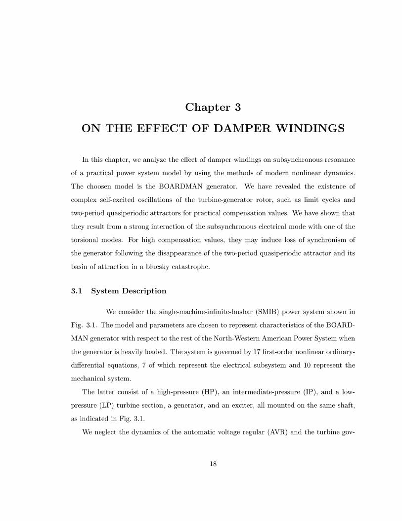
3.1 A schematic diagram for a series capacitor-compensated single machine power
system. The mechanical system consists of a high-pressure (HP), an intermediate-
pressure (IP), and a low-pressure (LP) turbine section, a generator (G), and
an exciter (Ex). . . . . . . . . . . . . . . . . . . . . . . . . . . . . . . . . . 19
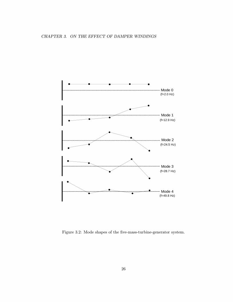
3.2 Mode shapes of the five-mass-turbine-generator system. . . . . . . . . . . . 26
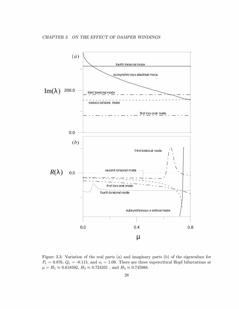
3.3 Variation of the real parts (a) and imaginary parts (b) of the eigenvalues for
Pe = 0.876, Qe = -0.115, and vt = 1.09. There are three supercritical Hopf
bifurcations at µ = H1 ≈ 0.618592, H2 ≈ 0.724331 , and H3 ≈ 0.745988. . . 28
3.4 Bifurcation diagram showing variation of the generator rotor angle δr with
the compensation level µ. The solid lines denote sinks and the dashed lines
denote unstable foci. . . . . . . . . . . . . . . . . . . . . . . . . . . . . . . 30
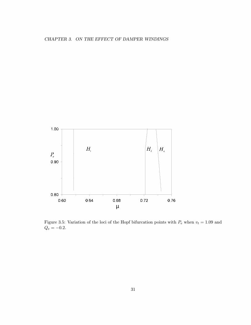
3.5 Variation of the loci of the Hopf bifurcation points with Pe when vt = 1.09
and Qe = −0.2. . . . . . . . . . . . . . . . . . . . . . . . . . . . . . . . . . 31
3.6 The influence of varying Qe on the locations of the Hopf bifurcations in
the Pe − µ plane for vt = 1.09. The solid lines correspond to Qe = 0.45, the
dashed lines correspond to Qe = 0.15, and the dashed-dotted lines correspond
to Qe = −0.2. . . . . . . . . . . . . . . . . . . . . . . . . . . . . . . . . . . 33
vii

LIST OF FIGURES
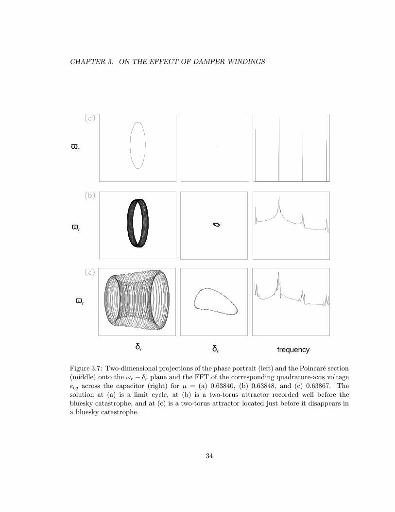
3.7 Two-dimensional projections of the phase portrait (left) and the Poincare
section (middle) onto the ωr − δr plane and the FFT of the corresponding
quadrature-axis voltage ecq across the capacitor (right) for µ = (a) 0.63840,
(b) 0.63848, and (c) 0.63867. The solution at (a) is a limit cycle, at (b)
is a two-torus attractor recorded well before the bluesky catastrophe, and
at (c) is a two-torus attractor located just before it disappears in a bluesky
catastrophe. . . . . . . . . . . . . . . . . . . . . . . . . . . . . . . . . . . . 34
3.8 Time traces of the generator rotor angle δr and frequency ωr at µ = (a)
0.63840, (b) 0.63848, and (c) 0.63867. . . . . . . . . . . . . . . . . . . . . . 35
3.9 Time histories of the generator rotor speed ωr (in rad/sec) and angle δr (in
rad) at µ = 0.63868, which is slightly larger than µ = C1 ≈ 0.63867 at which
the bluesky catastrophe occurs. . . . . . . . . . . . . . . . . . . . . . . . . . 36
3.10 Variation of the real and imaginary parts of the eigenvalues with µ when
Pe = 0.876, Qe = −0.115, vt = 1.09, and RQ = 0.006. There is only one Hopf
bifurcation at µ ≈ 0.422172. . . . . . . . . . . . . . . . . . . . . . . . . . . . 41
3.11 Variation of the real and imaginary parts of the eigenvalues with µ when RQ
= 0.015. . . . . . . . . . . . . . . . . . . . . . . . . . . . . . . . . . . . . . . 42
3.12 Variation of the maximum real parts of the eigenvalues with RQ for three
values of µ : µ1 = 0.422127, µ2 = 0.422027, and µ3 = 0.421027. . . . . . . 43
3.13 Bifurcation diagram showing variation of the generator rotor angle δr with
the compensation level µ. The solid line denotes sinks and the dashed line
denotes unstable foci. . . . . . . . . . . . . . . . . . . . . . . . . . . . . . . 44
viii
LIST OF FIGURES
3.14 Two-dimensional projections of the phase portrait onto the ωr−δr plane(left),the FFT of the corresponding generator rotor angle δr (middle), and the
time traces of the generator rotor angle δr (right) at µ = (a) 0.406425, (b)
0.411385, and (c) 0.417424. The solution at (a) is a limit cycle, at (b) is
a two-torus attractor recorded well before the bluesky catastrophe, and at
(c) is a two-torus attractor located just before it disappears in a bluesky
catastrophe. . . . . . . . . . . . . . . . . . . . . . . . . . . . . . . . . . . . 45
3.15 Time histories of the generator rotor speed ωr (in rad/sec) and angle δr (in
rad) at µ = 0.418576, which is slightly larger than C ≈ 0.418574 at which
the bluesky catastrophe that occurs. . . . . . . . . . . . . . . . . . . . . . . 46
3.16 Variation of the real and imaginary parts of the eigenvalues with µ in the
case of d-axis damper windings when RD= 0.0037. . . . . . . . . . . . . . . 47
3.17 Bifurcation diagram showing variation of the generator rotor angle δr with
the compensation level µ. The solid line denotes sinks and the dashed line
denotes unstable foci. . . . . . . . . . . . . . . . . . . . . . . . . . . . . . . 48
3.18 Two-dimensional projections of the phase portrait onto the ωr−δr plane(left),the FFT of the corresponding generator rotor angle δr (middle), and the time
traces of the generator rotor angle δr (right) at µ = (a) 0.5738, (b) 0.59295,
and (c) 0.59585. The solution at (a) is a limit cycle, at (b) is a two-torus
attractor recorded well before the bluesky catastrophe, and at (c) is a two-
torus attractor located just before it disappears in a bluesky catastrophe. . 50
3.19 The time history of the generator rotor angle δr (in rad) at µ = 0.60787,
which is slightly larger than C ≈ 0.60785 at which the bluesky catastrophe
that occurs. . . . . . . . . . . . . . . . . . . . . . . . . . . . . . . . . . . . . 51
3.20 Variation of the real and imaginary parts of the eigenvalues with µ in the
case of d-and-q axes damper windings when RQ = 0.006 and RD = 0.0037. 52
ix
LIST OF FIGURES
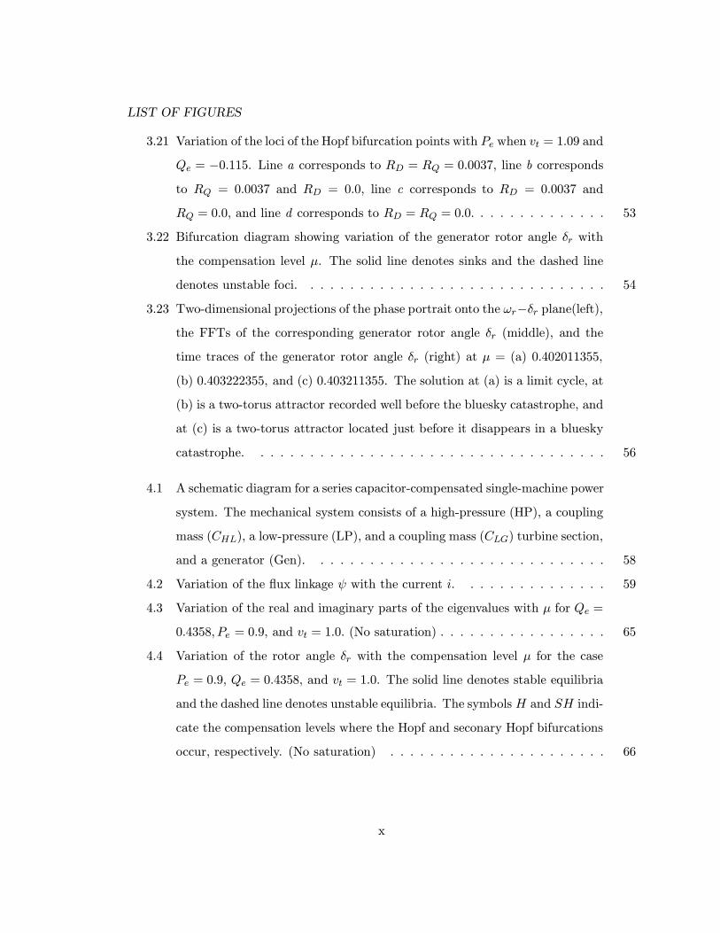
3.21 Variation of the loci of the Hopf bifurcation points with Pe when vt = 1.09 and
Qe = −0.115. Line a corresponds to RD = RQ = 0.0037, line b corresponds
to RQ = 0.0037 and RD = 0.0, line c corresponds to RD = 0.0037 and
RQ = 0.0, and line d corresponds to RD = RQ = 0.0. . . . . . . . . . . . . . 53
3.22 Bifurcation diagram showing variation of the generator rotor angle δr with
the compensation level µ. The solid line denotes sinks and the dashed line
denotes unstable foci. . . . . . . . . . . . . . . . . . . . . . . . . . . . . . . 54
3.23 Two-dimensional projections of the phase portrait onto the ωr−δr plane(left),the FFTs of the corresponding generator rotor angle δr (middle), and the
time traces of the generator rotor angle δr (right) at µ = (a) 0.402011355,
(b) 0.403222355, and (c) 0.403211355. The solution at (a) is a limit cycle, at
(b) is a two-torus attractor recorded well before the bluesky catastrophe, and
at (c) is a two-torus attractor located just before it disappears in a bluesky
catastrophe. . . . . . . . . . . . . . . . . . . . . . . . . . . . . . . . . . . . 56
4.1 A schematic diagram for a series capacitor-compensated single-machine power
system. The mechanical system consists of a high-pressure (HP), a coupling
mass (CHL), a low-pressure (LP), and a coupling mass (CLG) turbine section,
and a generator (Gen). . . . . . . . . . . . . . . . . . . . . . . . . . . . . . 58
4.2 Variation of the flux linkage ψ with the current i. . . . . . . . . . . . . . . 59
4.3 Variation of the real and imaginary parts of the eigenvalues with µ for Qe =
0.4358, Pe = 0.9, and vt = 1.0. (No saturation) . . . . . . . . . . . . . . . . . 65
4.4 Variation of the rotor angle δr with the compensation level µ for the case
Pe = 0.9, Qe = 0.4358, and vt = 1.0. The solid line denotes stable equilibria
and the dashed line denotes unstable equilibria. The symbols H and SH indi-
cate the compensation levels where the Hopf and seconary Hopf bifurcations
occur, respectively. (No saturation) . . . . . . . . . . . . . . . . . . . . . . 66
x

LIST OF FIGURES
4.5 Variation of the loci of the Hopf bifurcation points with Pe and µ for vt = 1.0
and Qe = 0.4358. . . . . . . . . . . . . . . . . . . . . . . . . . . . . . . . . 67
4.6 Two-dimensional projections of the phase portrait onto the ωr−δr plane(left),the FFT of the corresponding generator rotor angle δr (middle), and the time
traces of the generator rotor angle δr (right) at µ = (a) 0.880981, (b) 0.88598,
and (c) 0.889760. The solution at (a) is a limit cycle, at (b) is a two-torus
attractor recorded well before the bluesky catastrophe, and at (c) is a two-
torus attractor located just before it disappears in a bluesky catastrophe. . 69
4.7 Time histories of the generator rotor speed ωr (in rad/sec) and angle δr (in
rad) in the vicinity of the bluesky catastrophe that occurs at C ≈ 0.89976. 70
4.8 Variation of the real and imaginary parts of the eigenvalues with µ for Qe =
0.438, Pe = 0.9, and vt = 1.0. (With saturation) . . . . . . . . . . . . . . . . 71
4.9 Variation of the rotor angle δr with the compensation level µ for the case Pe =
0.9, Qe = 0.4358, and vt = 1.0. The solid line denotes stable equilibria and
the dashed line denotes unstable equilibria. The symbols H and SH indicate
the compensation levels at which the Hopf and secondary Hopf bifurcations
occur. (With saturation) . . . . . . . . . . . . . . . . . . . . . . . . . . . . 72
4.10 Two-dimensional projections of the phase portrait onto the ωr−δr plane(left),the FFT of the corresponding generator rotor angle δr (middle), and the
time traces of the generator rotor angle δr (right) at µ = (a) 0.842351, (b)
0.848651, and (c) 0.887651. The solution at (a) is a limit cycle, at (b) is
a two-torus attractor recorded well before the bluesky catastrophe, and at
(c) is a two-torus attractor located just before it disappears in a bluesky
catastrophe. . . . . . . . . . . . . . . . . . . . . . . . . . . . . . . . . . . . 75
4.11 Time histories of the generator rotor speed ωr (in rad/sec) and angle δr (in
rad) in the vicinity of the bluesky catastrophe that occurs at C ≈ 0.8976. . 76
5.1 A block diagram for a generator excitation control system. . . . . . . . . . 78
xi

LIST OF FIGURES
5.2 A static excitation system of the ST3 type, which is a compound source
controlled rectifier exciter (GENEREX). . . . . . . . . . . . . . . . . . . . 80
5.3 a) Power system stabilizer (PSS) and b) nonlinear controller. . . . . . . . . 81
5.4 Variation of the real and imaginary parts of the eigenvalues with µ for Qe =
0.4358 and Pe = 0.9, (Without PSS) . . . . . . . . . . . . . . . . . . . . . . 86
5.5 Bifurcation diagram showing variation of the generator rotor angle δr with the
compensation level µ. Line 2 corresponds to the case without the excitation
system and the PSS, and line 1 corresponds to the case with the excitation
system only. The solid lines denote sinks and the dashed lines denote unstable
foci. . . . . . . . . . . . . . . . . . . . . . . . . . . . . . . . . . . . . . . . . 88
5.6 Variation of the real and imaginary parts of the eigenvalues with µ for Qe =
0.4358 and Pe = 0.9, (With PSS) . . . . . . . . . . . . . . . . . . . . . . . . 91
5.7 Bifurcation diagram showing variation of the generator rotor angle δr with the
compensation level µ. Line 2 corresponds to the case without the excitation
system and the PSS, and line 1 corresponds to the case with the excitation
system and the PSS. The solid lines denote sinks and the dashed lines denote
unstable foci. . . . . . . . . . . . . . . . . . . . . . . . . . . . . . . . . . . . 93
5.8 Variation of the loci of the Hopf bifurcation points with kj when Pe = 0.9
and Qe = −0.2, and τa = 0.4. . . . . . . . . . . . . . . . . . . . . . . . . . . 94
5.9 Variation of the loci of the Hopf bifurcation points with τa when Pe = 0.9
and Qe = −0.2, and kj = 200. . . . . . . . . . . . . . . . . . . . . . . . . . . 95
5.10 Variation of a, the amplitude of the limit-cycle born at H, with the nonlinear
controller gain k. . . . . . . . . . . . . . . . . . . . . . . . . . . . . . . . . 97
xii

Chapter 1
INTRODUCTION
1.1 Problem Definition and Literature Review
1.1.1 Subsynchronous Resonance Problem
In power systems, series capacitors are being installed by many electric utilities to
increase the power transfer capability of the transmission lines as well as to improve the
stability of these systems. However, this introduces problems together with the benefits,
namely the occurrence of undesirable oscillations that may lead to the destruction of the
shaft of the turbine or the loss of synchronism of the generator. This phenomenon has been
given the name subsynchronous resonance or SSR for short[1].
The phenomenon of SSR was brought to general attention in connection with the two
damages that occurred to the turbine-generator shafts at the Mohave Generating Station
in southern Nevada in the United States of America in December of 1970 and October of
1971. These two failures have been analyzed by Walker et al. [2], among others. Walker
and his colleagues found that the failures occurred in the shaft section between the gen-
erator and the exciter of the main generator collector are due to torsional fatigue. They
concluded that a conducting path was generated from each collector ring through the insu-
lating sleeves to the shaft. Heavy current flowing through the double ground then eroded
large pockets of metal from the shaft and collector rings. Analysis of line current oscil-
lograms taken during the disturbance indicate the presence of appreciable magnitudes of
currents at subsynchronous frequency. These currents produced subsynchronous torques
on the generator of approximately the same magnitude, but at a slip frequency that was
very nearly equal to the frequency of the second torsional mode of the shaft system. The
1

CHAPTER 1. INTRODUCTION
latter involved, essentially, the exciter-alternator shaft, which was oscillating mechanically
against the remaining shaft inertial elements, thereby causing the destruction of the shaft
of the turbine-generator system.
1.1.2 Types of SSR
There are many ways in which the system and the generator may interact under sub-
synchronous resonance conditions. Farmer et al. [3], in their analysis carried out during the
Navajo project, identified three types of subsynchronous resonance. They have been called
induction generator effect, torsional interaction effect, and transient torque effect. These
three interactions, which are of particular interest, are briefly discussed next.
As mentioned in [4-9], the induction generator effect is caused by self-excitation of
the synchronous generators when the resistance of the rotor to the subsynchronous current,
viewed from the armature terminal, becomes negative. The network also presents a positive
resistance to these same currents. However, if the negative resistance of the generator is
greater in magnitude than the positive resistance of the network at the natural frequencies,
there will be sustained subsynchronous currents.
The torsional interaction effect occurs when the slip frequency, which is equal to the
difference between the synchronous and subsynchronous frequencies (i.e., f − fn), is close to
a torsional mode frequency ”fm” of the shaft. Consequently, generator-rotor oscillations can
build up to induce armature voltage components of subsynchronous and supersynchronous
frequencies [8]. The subsynchronous frequency voltage is phased to sustain the subsyn-
chronous torque. If the latter equals or exceeds the inherent mechanical damping torque
of the rotating system, the system will become self-excited. As a result, severe torque
amplification can occur, resulting in damage to the shaft of the machine.
As for transient torques, they are not self-excited. They are rather induced by system
disturbances, which tend to excite the natural frequencies of the network. This causes the
generator-turbine masses to oscillate relative to one another at one or more of their natural
frequencies depending on the system disturbance.
2

CHAPTER 1. INTRODUCTION
1.1.3 SSR Countermeasures
As a solution to SSR problems, several countermeasures have been applied and more
have been suggested in the literature. We will summarize the ones proposed by Farmer et al.
[3] and the General Electric system. Regarding the elimination of the induction generator
effect, they recommend that the generator be equipped with poleface amortisseurs. As for
the mitigation of the torsional interaction effect, they suggest the installation of filters in
series with the generator to increase the circuit resistance for each torsional mode. Finally,
to reduce the transient torque on the turbine-generator shafts to the level that shaft fracture
may not occur for any single transient incident, they suggest the adoption of a capacitor
dual gap flashing scheme. Because of the high amplitudes of oscillations and the fast torque
build up, transient torque problems require more extreme and costly countermeasures than
those needed to mitigate the self-excitation cases.
A linear excitation system controller, namely GENEREX, has been implemented by
Beagles et al. [10]. This type of controller is used to enlarge the stability region. In this
DISSERTATION, in addition to the linear controller, we design a nonlinear controller to
reduce the amplitudes of the nonlinear oscillations in the unstable region.
1.1.4 Analytical Tools
There are several techniques proposed to study the phenomenon of SSR. They can be
classified into two categories, namely linear and nonlinear techniques. The most common of
these techniques are frequency scanning, eigenvalue analysis, and ElectroMagnetic Transient
Program (EMTP) analysis (see Anderson et al. [8] and [11-13], among others). The first
two methods are linear and the third one is nonlinear.
The frequency scanning technique has been utilized by Ballance and Goldberg [1], Kil-
gore et al. [12], Farmer et al. [3], Rana et al. [13], and Edris [11], among others. This
method has been widely used in North America for at least a preliminary analysis of the
SSR problem. It is particularly effective in the study of the induction generator effect. It
3

CHAPTER 1. INTRODUCTION
computes, as a function of frequency, the equivalent resistance and reactance that are seen
looking into the network from a point behind the stator winding of a particular generator.
While being relatively inexpensive for large systems, the frequency scanning method cannot
identify self-excited torsional oscillations. For analyzing this type of oscillations, one resorts
to eigenvalue analysis.
The eigenvalue analysis technique has been utilized by Yu [14], Fouad and Khu [15],
Walker et al. [2], Yan and Yu [16], Anderson et al. [8], and Iravani and Edris, [17], to
cite a few. It is performed with the network and the generators modeled in a linearized
system of differential equations. It is a very attractive technique because it provides both
the frequencies of oscillation and the damping at each frequency. However, the eigenvalue
analysis technique is relatively expensive, especially for large power systems.
To avoid linearizing the differential equations, Gross and Hall [9] and Edris [11], among
others, have used EMTP. The latter numerically integrates the set of nonlinear differential
equation that govern the power system. EMTP is a full three-phase model of the system
with much more detailed modeling of the transmission lines, cables, machines, and special
devices, such as series capacitors, with complex bypass switching arrangements. Moreover,
EMTP permits nonlinear modeling of complex system components. It is, therefore, well
suited for the analysis of SSR problems.
EMTP has also been used by several authors [9, 18-21] to invalidate the results pre-
dicted by the linearized theories, especially the eigenvalue analysis. The latter predicts that
disturbances to the power system decay below a critical compensation level µc at which a
complex conjugate pair of eigenvalues crosses the imaginary axis into the right-half of the
complex plane and exponentially grow above µc. In nonlinear dynamics, µc is known as
a Hopf bifurcation value. But, numerical simulations using EMTP demonstrate that the
nonlinearities put a cap on the exponential growth. This limitation of the linearized theories
has prompted a growing interest in nonlinear bifurcation methods.
In recent years, power system dynamics has been studied from the point of view of
geometric methods of nonlinear dynamics. The presence of different types of bifurcation
4

CHAPTER 1. INTRODUCTION
in power system models has been revealed. The most commonly encountered bifurcation
in these models is the Hopf bifurcation. Abed and Varaiya [22] were the first to spot
a subcritical Hopf bifurcation in a voltage stability model of a power system consisting
of a machine with an excitation system connected to an infinite busbar. Later, Dobson
and Chiang [23], Nayfeh et al. [24], Venkatasubramanian et al. [25], Ajjarapu and Lee
[26], among others, studied voltage stability by investigating the bifurcation of static and
dynamic solutions. Recently, Abed et al. [27], Ji and Venkatasubramian [28], and Nayfeh
et al. [29] showed that the birth or death of limit cycles from an equilibrium point gives rise
to oscillations that may undergo period multiplications, cyclic folds, and crises.
In the SSR area, Zhu [18] and Zhu et al. [20] were the first to employ bifurcation
methods to demonstrate the existence of a Hopf bifurcation in a single-machine-infinite-
busbar power system. They appealed to the Hopf bifurcation theorem to show that the
bifurcation is supercritical and, hence, it leads to the birth of a stable small-amplitude
limit cycle. They validated these results with numerical simulations obtained by using
EMTP. Zhu [18] found that, as the series compensation level increases, the limit cycle loses
stability with a complex conjugate pair of Floquet multipliers leaving the unit circle in the
complex plane away from the real axis. This indicates a two-period quasiperiodic (two-
torus) motion. She conjectured that the torus is unstable. In this DISSERTATION, we
show that the created two-torus is stable and that as the compensation level increases, it
loses stability in a bluesky catastrophe.
1.2 Objectives and Scope of the DISSERTATION
In this DISSERTATION, we concentrate on the second type of self-excitation, which
results from the interaction of the electrical subsynchronous mode with a torsional mode.
Bifurcation theory, Floquet theory, and the method of multiple scales [30] are used to investi-
gate the complex dynamics of a series capacitor compensated single-machine-infinite-busbar
power system. Two practical power system models are used, namely the BOARDMAN and
5

CHAPTER 1. INTRODUCTION
CHOLLA#4.
In the BOARDMAN model, the dynamics of the automatic voltage regulator (AVR),
the turbine governor, and the generator saturation are neglected. We consider two cases,
one without damper windings and the other one with. In the first case, we extend the work
of Zhu [18] by revealing the existence of not one but three supercritical Hopf bifurcations for
practical compensation values. We show that they result from the interaction of the elec-
trical subsynchronous mode with one of the mechanical modes of the system. In addition,
we use a combination of a two-point boundary-value scheme and Floquet theory to unveil
the presence of three secondary Hopf bifurcations. In their vicinity, the oscillations have
two incommensurate periods with bounded amplitudes, yielding two-period quasiperiodic
motions (two-torus). Finally, we show that these attractors grow in size until they collide
with their basins of attraction, resulting in their joint destruction in a bluesky catastrophe.
Above this level of compensation, the oscillations become unbounded and the generator
permanently loses synchronism. These scenarios are validated through time-domain simu-
lations obtained by integrating the differential equations that govern the system. We have
also studied the effects of the damper windings on SSR. We found that placing damper
windings on either the q-axis, or the d-axis, or both axes reduces the compensation level at
which the system loses stability via a Hopf bifurcation.
The effect of the generator saturation has been analyzed in another power system model,
namely the CHOLLA#4 model. Here, the dynamics of the turbine governor have been
neglected. When the saturation and automatic voltage regulator (AVR) are neglected, it
is shown that there is only one supercritical Hopf bifurcation point in the vicinity of which
there exist small stable limit cycles. As the compensation level of the line increases, the
limit cycles grow in size and then undergo a secondary Hopf bifurcation, which leads to
two-period quasiperiodic attractors. When the generator saturation is accounted for, it is
found that the supercritical Hopf bifurcation point occurs at a lower level of compensation,
implying a decrease in the positively damped region.
To move the Hopf bifurcation point to higher capacitor compensation values (i.e., to
6
CHAPTER 1. INTRODUCTION
enlarge the stability region), we have used a PSS-type linear controller that acts on the
excitation system. Moreover, to decrease the amplitudes of the nonlinear oscillations in
the unstable region, we have designed a nonlinear (quadratic) controller that injects an
additional stabilizing signal into the automatic voltage regulator (AVR). We note that, for
both the linear and nonlinear controllers, the input signal is the deviation of thr generator-
rotor frequency from the synchronous frequency.
1.3 Outline of the DISSERTATION
The DISSERTATION is organized as follows. Chapter 2 briefly reviews methods of
modern nonlinear dynamics, such as bifurcation and Floquet theories and the method of
multiple scales. Chapter 3 studies the effect of damper windings on the subsynchronous reso-
nance of the BOARDMAN model. Chapter 4 analyzes the effect of the generator saturation
on the SSR of the CHOLLA#4 model. In Chapter 5, mitigation of SSR in CHOLLA#4
through linear and nonlinear controllers is demonstrated. Finally, some conclusions and
recommendations for future work are given in Chapter 6.
7

Chapter 2
A REVIEW OF MODERN NONLINEARDYNAMICS
In this chapter, methods of modern nonlinear dynamics are briefly reviewed [30]. Specif-
ically, the constant solutions and their stability are analyzed using bifurcation theory. The
method of multiple scales [31] is implemented to find the normal form of the system near
the Hopf bifurcation points. Moreover, Floquet theory is employed to study the stability of
limit cycles.
2.1 Equilibrium Solutions
The equilibrium solutions or constant solutions of an autonomous system defined by
x = F(x;µ) (2.1)
where x is a state variables vector, x1, x2, ..., xn, n is an integer number, F is the field vector,
and µ is the control parameter of the system, correspond to
x = 0 (2.2)
By equating the right-hand side of Eq. (2.1) to zero, we end up with either linear or
nonlinear algebraic equations. If the function F in Eq. (2.1) is linear, then the system
is linear. So, it has only one constant solution, namely, the trivial solution if the system
matrix is nonsingular. In contrast, for a nonlinear system, there may be more than one
constant or equilibrium solution. Using a continuation scheme, discussed in Sec. 2.3, we
solve these equations as a function of the control parameter µ. The stability of this type of
solution is discussed next.
8

CHAPTER 2. A REVIEW OF MODERN NONLINEAR DYNAMICS
2.1.1 Stability of Equilibrium Solutions
The stability of an equilibrium solution x0 at µ = µ0 depends on the eigenvalues of
the Jacobian matrix J of the system (2.1), which is the matrix of first partial derivatives.
Consider a small disturbance y to the equilibrium solution x0, so that
x(t) = x0 + y(t). (2.3)
Substituting Eq. (2.3) into Eq. (2.1) gives
y = F(x0 + y;µ0). (2.4)
Using a Taylor series expansion around x0 and keeping only the linear terms in y, one
obtains
y = F(x0;µ0) +DxF(x0;µ0)y + ... (2.5)
However, at the equilibrium solution x0, F(x0;µ0) = 0. So, Eq. (2.5) becomes
y ≈ DxF(x0;µ0)y = Jy (2.6)
The eigenvalues of the constant matrix J provide information about the local stability
of the equilibrium solution x0. An equilibrium solution is classified as hyperbolic or non-
hyperbolic. If all of the eigenvalues of J have nonzero real parts, then the corresponding
equilibrium solution is called a hyperbolic fixed point; otherwise, it is called a nonhyperbolic
fixed point. The hyperbolic fixed points are of three types: stable nodes, unstable nodes,
and saddle points. A fixed point is called a stable node or a sink if all of the eigenvalues
of J have negative real parts. If the matrix J associated with a stable node has complex
eigenvalues, the stable node is also called a stable focus. An equilibrium point is called an
unstable node or a source if one or more of the eigenvalues of J have positive real parts. An
unstable node is called an unstable focus if the associated matrix J has complex eigenvalues.
9
CHAPTER 2. A REVIEW OF MODERN NONLINEAR DYNAMICS
An equilibrium point is a saddle if some, but not all, of the eigenvalues have positive real
parts while the rest of them have negative real parts. On the other hand, a nonhyperbolic
fixed point is unstable if one or more of the eigenvalues of J have positive real parts. It is
said to be marginally stable if some of the eigenvalues of J have negative real parts while
the rest of them have zero real parts. It is called a center if all the eigenvalues of J are
purely imaginary and nonzero.
2.2 Bifurcation Theory
Bifurcation is a French word that has been introduced into nonlinear dynamics by
Poincare. It is used to indicate a qualitative change in the dynamics of a system, such
as the number and type of solutions under the variation of one or more parameters on
which the system in question depends. In bifurcation problems, it is useful to consider
a space formed by using the state variables and the control parameters, called the state-
control space. In this space, locations at which bifurcations occur are called bifurcation
points.
In this DISSERTATION, we are mainly concerned with local bifurcation of fixed points
and limit cycles of an autonomous system of differential equations as a function of scalar
control parameters.
2.2.1 Local Bifurcations of Fixed Points
Local bifurcation is a qualitative change occurring in the neighborhood of a fixed point
or a periodic solution of the system. When a single control parameter is varied, a fixed point
of an autonomous system, such as the one given by (2.1), can lose stability through one
of the following bifurcations: saddle-node bifurcation, pitchfork bifurcation, transcritical
bifurcation, and Hopf bifurcation.
At bifurcation points associated with saddle-node, pitchfork, and transcritical bifurca-
tions, only branches of fixed points or static solutions meet. Hence, these three bifurcations
10

CHAPTER 2. A REVIEW OF MODERN NONLINEAR DYNAMICS
are classified as static bifurcations. In contrast, branches of fixed points and periodic solu-
tions meet at a hopf bifurcation point. Hence, a Hopf bifurcation is classified as a dynamic
bifurcation.
Let us now give the definition of a static and Hopf bifurcation. A static bifurcation of
a fixed point of (2.1) occurs at a certain value of µ, say µ = µ0, if the following conditions
are satisfied:
1- F(x0;µ0) = 0
2- The Jacobian matrix DxF evaluated at (x0;µ0) has a zero eigenvalue while all of its
other eigenvalues have negative real parts.
It is clear that the first condition ensures that the considered solution is a fixed point of
(2.1), while the second condition implies that this fixed point is a nonhyperbolic fixed point.
One should note that these conditions are necessary but not sufficient.
A Hopf bifurcation of a fixed point of (2.1) occurs at a certain value of µ, say µ = µ0,
if the following conditions are satisfied:
1- F(x0;µ0) = 0
2- The Jacobian matrix DxF evaluated at (x0;µ0) has a pair of purely imaginary eigen-
values ±jω while all of its other eigenvalues have negative real parts.
3- For µ = µ0, let the analytic continuation of the pair of purley imaginary eigenvalues
be (λ± jω). Then dλdµ 6= 0 at µ = µ0.
The first two conditions imply that the fixed point undergoing the bifurcation is a nonhy-
perbolic fixed point. The third condition implies a transversal or nonzero speed crossing of
the imaginary axis and, hence, it is called a transversality condition. When all of the above
three conditions are satisfied, a periodic solution of period (2π/ω) may be born at (x0;µ0).
11
CHAPTER 2. A REVIEW OF MODERN NONLINEAR DYNAMICS
2.2.2 Continuation Schemes
Continuation schemes are used to determine how solutions of (2.1) vary with a cer-
tain parameter. These schemes are based on the Implicit Function Theorem. There are
two categories of continuation schemes. The first category consists of predictor-corrector
methods, which approximately follow a branch of solutions. The second category consists
of piecewise-linear or simplical methods, which exactly follow a piecewise-linear curve that
approximates a branch of solutions.
Among the above two categories, there are many types of continuation methods, such as
the sequential scheme, the Davidenko Newton-Raphson scheme, the arclength scheme, and
the pseudo-arclength scheme. In the arclength scheme, the arclength s along a branch of
solutions is used as the continuation parameter. So, x and µ are considered to be function
of s; that is, x = x(s) and µ = µ(s). This parameterization is useful in carrying out a
continuation along a path with a saddle-node bifurcation (turning point). On the path
parameterized by the arclength s, we seek x and µ such that
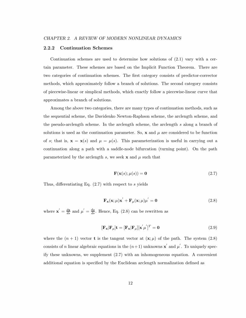
F(x(s);µ(s)) = 0 (2.7)
Thus, differentiating Eq. (2.7) with respect to s yields
Fx(x;µ)x′+ Fµ(x;µ)µ
′= 0 (2.8)
where x′= dx
ds and µ′= dµ
ds . Hence, Eq. (2.8) can be rewritten as
[Fx|Fµ]t = [Fx|Fµ][x′µ
′]T = 0 (2.9)
where the (n + 1) vector t is the tangent vector at (x;µ) of the path. The system (2.8)
consists of n linear algebraic equations in the (n+1) unknowns x′and µ
′. To uniquely spec-
ify these unknowns, we supplement (2.7) with an inhomogeneous equation. A convenient
additional equation is specified by the Euclidean arclength normalization defined as
12

CHAPTER 2. A REVIEW OF MODERN NONLINEAR DYNAMICS
x′Tx
′+ µ
′2= 1 (2.10)
The initial conditions for Eqs. (2.8) and (2.10) are given by x = x0 and µ = µ0 at s = 0.
If the Jacobian matrix Fx is nonsingular and Fµ is a zero vector, Eqs. (2.8) and (2.10) yield
[x′Tµ
′] = ±[0 0 . . . 0 1] (2.11)
If Fx is nonsingular and Fµ is a nonzero vector, one can solve Eqs. (2.8) and (2.10)
to determine the tangent vector t as follows. First, solve the system of n linear algebraic
equations
Fx(x;µ)Z = −Fµ(x;µ) (2.12)
for the vector Z. Then, owing to the linearity of Eq. (2.8) in x′and µ
′, we write
x′= Zµ
′(2.13)
where µ′is still unknown. Substituting Eq. (2.13) into the arclength Eq. (2.10) yields
µ′= ± 1√
(1 + ZTZ)(2.14)
where the plus and minus signs determine the direction of the continuation. Having deter-
mined the tangent vector t, we use it to predict the values of x and µ at s = ∆s according
to x = x0 + x′∆s and µ = µ0 + µ
′∆s. These predicted values can be corrected by using
a Newton-Raphson procedure, and the predictor-corrector scheme is continued until the
branch is traced. The choice of the step size ∆s should be such that the initial guess or
estimate is within the radius of convergence of the corrector. The step size may have to be
adaptively varied during the continuation.
13

CHAPTER 2. A REVIEW OF MODERN NONLINEAR DYNAMICS
2.2.3 The Normal Form Near a Hopf Bifurcation Point
To determine the normal form of Eq. (2.1) near a Hopf bifurcation value Hi, we let
x− x0 = εy and µ−Hi = ε2µ (2.15)
where x0 is the fixed point at Hi and ε is a small dimensionless parameter that is used as
a bookkeeping device. Substituting Eq. (2.15) into Eq. (2.1) and expanding the result for
small ε, we obtain
y = Jy + εQ(y,y) + ε2C(y,y,y) + ε2µBy + · · · (2.16)
Here J is the n×n Jacobian matrix of F evaluated at (x0,Hi), B is a n×n constant matrix,Q(y,y) is generated by a vector-valued symmetric bilinear form Q(u,v), and C(y,y,y) is
generated by a vector-valued symmetric trilinear form C(u,v,w). At µ = Hi, J has a pair
of purely imaginary eigenvalues ±jω with the remaining eigenvalues in the left-half plane.
Using the method of multiple scales [31 and 32], we seek a third-order expansion in the
form
y(t; ε) = y(T0, τ2) + εy2(T0, τ2) + ε2y3(T0, τ2) + · · · (2.17)
where T0 = t and τ2 = ε2t. Substituting Eq. (2.17) into Eq. (2.16) and equating coefficients
of like powers of ε, we obtain equations governing y1,y2, and y3. The non-decaying solution
of y1 is written as
y1 = A(τ2)pejωT0 + A(τ2)pe
−jωT0 (2.18)
where p is the right eigenvector of J corresponding to the eigenvalue jω. Then, the solution
of the second-order problem is expressed as
y2 = 2z0AA+ 2z2A2e2jωT0 + cc (2.19)
where cc is the complex conjugate of the preceding terms and z0 and z2 are the solutions
of the algebraic systems of equations
Jz0 = −1
2Q(p,p) (2.20)
14
CHAPTER 2. A REVIEW OF MODERN NONLINEAR DYNAMICS
(2jω − J)z2 =1
2Q(p,p) (2.21)
Finally, eliminating the secular terms from y3 yields
A′ = µ(β1 + jβ3)A+ 4(β2 + jβ4)A2A (2.22)
where
β1 + jβ3 = qTBp (2.23)
β2 + jβ4 = 2qTQ(p, z0) + qTQ(p, z2) +3
4qTC(p,p,p) (2.24)
and q is the left eigenvector of J corresponding to the eigenvalue jω. It is normalized so
that qTp = 1. Letting A = 12a exp(jθ) and separating real and imaginary parts, we find
that the real part is given by
a′ = (µ−Hi)β1a+ β2a3 (2.25)
2.2.4 Floquet Theory
To study the stability of a periodic solution X(t) of least period T of the system of n
autonomous first-order nonlinear equations (2.1), we let
X(t) = X(t) + u(t) (2.26)
Substituting (2.26) into (2.1) and linearizing in u(t) leads to
u = DxF(X;µ)u (2.27)
where DxF(X;µ) is the Jacobian matrix of F evaluated at x = X. Then, we solve the linear
system of equations (2.27) to determine n linearly independent solutions u1,u2, · · · ,un and
form the fundamental matrix
U = [u1 u2 · · · un] (2.28)
Usually, one chooses the initial conditions such that
U(0) = I (2.29)
15
CHAPTER 2. A REVIEW OF MODERN NONLINEAR DYNAMICS
where I is the n × n identify matrix. Then, the stability of X(t) is ascertained from the
eigenvalues ρ1, ρ2, · · · , ρn of the so-called monodromy matrix U(T ). These eigenvalues are
called the Floquet multipliers. One of these multipliers is always unity for an autonomous
system [19]. If all of the other multipliers are inside the unit circle in the complex plane,
the limit cycle X(t) is stable; otherwise, it is unstable.
2.2.5 Local Bifurcations of Periodic Solutions
When a single control parameter varies, a periodic solution of an autonomous system,
such as the one given by Eq. (2.1), can lose stability through one of the following bifurca-
tions: transcritical, symmetry-breaking, cyclic-fold, period doubling, and secondary Hopf
bifurcations. The resulting solution depends on how the Floquet multipliers leave the unit
circle. There are three possible scenarios. First, a Floquet multiplier leaves the unit circle
along the real axis through +1, resulting in either a trancritical, or a symmetry-breaking,
or a cyclic-fold bifurcation. At a cyclic-fold bifurcation, stable limit cycle collides with
an unstable limit cycle, resulting in their annihilation. In a transcritical bifurcation, two
branches of stable and unstable cycles coexist below the bifurcation value and exchange sta-
bility after the bifurcation. In a symmetry-breaking bifurcation, the symmetry of the limit
cycle is broken. At such a bifurcation, a branch of symmetric limit cycles meets branches
of asymmetric limit cycles.
Second, a Floquet multiplier leaves the unit circle through −1, resulting in a period-
doubling bifurcation. A branch of stable limit cycles that exist before the bifurcation µc
continues as unstable branch of limit cycles after µc. If the bifurcation is supercritical,
a new branch of stable period-doubled solutions is created. If the point is subcritical, a
branch of unstable period-doubled solutions is destroyed.
Third, two complex conjugate Floquet multipliers leave the unit circle away from the
real axis, resulting in a secondary Hopf or Neimark bifurcation. As mentioned earlier, the
Hopf bifurcation of a fixed point of an autonomous system, such as the one given by Eq.
(2.1), leads to a periodic solution of this system. In other words, the Hopf bifurcation
16
CHAPTER 2. A REVIEW OF MODERN NONLINEAR DYNAMICS
introduces a new frequency to the system in addition to the first one. The Hopf bifurcation
of a periodic solution, called secondary Hopf bifurcation, produces either a periodic or a two-
period quasiperiodic solution, depending on whether the two frequencies are commensurate
or not.
17
Chapter 3
ON THE EFFECT OF DAMPER WINDINGS
In this chapter, we analyze the effect of damper windings on subsynchronous resonance
of a practical power system model by using the methods of modern nonlinear dynamics.
The choosen model is the BOARDMAN generator. We have revealed the existence of
complex self-excited oscillations of the turbine-generator rotor, such as limit cycles and
two-period quasiperiodic attractors for practical compensation values. We have shown that
they result from a strong interaction of the subsynchronous electrical mode with one of the
torsional modes. For high compensation values, they may induce loss of synchronism of
the generator following the disappearance of the two-period quasiperiodic attractor and its
basin of attraction in a bluesky catastrophe.
3.1 System Description
We consider the single-machine-infinite-busbar (SMIB) power system shown in
Fig. 3.1. The model and parameters are chosen to represent characteristics of the BOARD-
MAN generator with respect to the rest of the North-Western American Power System when
the generator is heavily loaded. The system is governed by 17 first-order nonlinear ordinary-
differential equations, 7 of which represent the electrical subsystem and 10 represent the
mechanical system.
The latter consist of a high-pressure (HP), an intermediate-pressure (IP), and a low-
pressure (LP) turbine section, a generator, and an exciter, all mounted on the same shaft,
as indicated in Fig. 3.1.
We neglect the dynamics of the automatic voltage regular (AVR) and the turbine gov-
18

CHAPTER 3. ON THE EFFECT OF DAMPER WINDINGS
AAAAAAAAAAAAAAAAAAAAAAAAAAAAAAAAAAAAAAAA
AAAAAAAAAAAAAAAAAAAAAAAAAAAAAAAAAAAAAAAA
AAAAAAAAAAAAAAAAAAAA
AAAAAAAAAAAAAAAAAAAAAAAAAAAAAAAAAAAAAAAA
AAAAAAAAAAAAAAAAAAAAAAAAAAAAAAAAAAAAAAAA
AAAAAAAAAAAAAAAAAAAA
AAAAAAAAAAAAAAAAAAAAAAAAAAAAAAAAAAAAAAAA
AAAAAAAAAAAAAAAAAAAAAAAAAAAAAAAAAAAAAAAA
AAAAAAAAAAAAAAAAAAAAAAAAAAAAAA
AAAAAAAAAAAAAAAAAAAAAAAAAAAAAAAAAAAAAAAA
AAAAAAAAAAAAAAAAAAAAAAAAAAAAAAAAAAAAAAAA
AAAAAAAAAAAAAAAAAAAAAAAAAAAAAA
AAAAAAAAAAAAAAAAAAAAAAAAAAAAAAAAAAAAAAAA
AAAAAAAAAAAAAAAAAAAAAAAAAAAAAAAAAAAAAAAA
AAAAAAAAAAAAAAAAAAAAAAAAAAAAAA
AAAAAAAAAAAA
AAA
AAAAAAAAAAAA
AAA
HP IP LP G Ex
RlX
l
Xc
vo
1 2 3 4 5
Figure 3.1: A schematic diagram for a series capacitor-compensated single machine powersystem. The mechanical system consists of a high-pressure (HP), an intermediate-pressure(IP), and a low-pressure (LP) turbine section, a generator (G), and an exciter (Ex).
ernor and include the dynamics of the damper windings on the q-and d-axes. Using the
direct and quadrature d − q axes and Park’s transformation, one can write the equations
describing the system as follows [14]:
(a) Machine:
dψddt
= ωb (vd +Raid + ωrψq) (3.1)
dψqdt
= ωb (vq +Raiq − ωrψd) (3.2)
dψfdt
= ωb (vf −Rf if ) (3.3)
dψQdt
= ωb (−RQiQ) (3.4)
dψDdt
= ωb (−RDiD) (3.5)
19
CHAPTER 3. ON THE EFFECT OF DAMPER WINDINGS
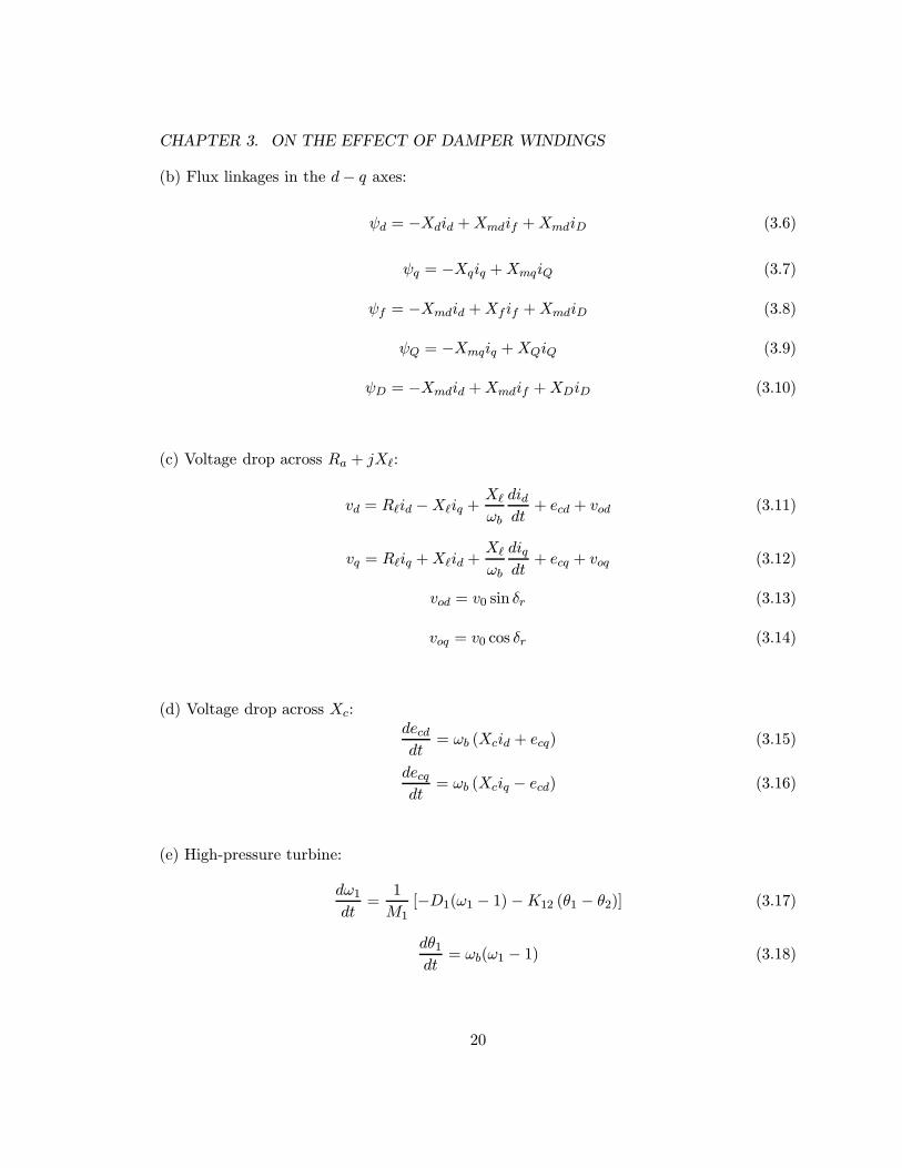
(b) Flux linkages in the d− q axes:
ψd = −Xdid +Xmdif +XmdiD (3.6)
ψq = −Xqiq +XmqiQ (3.7)
ψf = −Xmdid +Xf if +XmdiD (3.8)
ψQ = −Xmqiq +XQiQ (3.9)
ψD = −Xmdid +Xmdif +XDiD (3.10)
(c) Voltage drop across Ra + jX`:
vd = R`id −X`iq +X`
ωb
diddt
+ ecd + vod (3.11)
vq = R`iq +X`id +X`
ωb
diqdt
+ ecq + voq (3.12)
vod = v0 sin δr (3.13)
voq = v0 cos δr (3.14)
(d) Voltage drop across Xc:decddt
= ωb (Xcid + ecq) (3.15)
decqdt
= ωb (Xciq − ecd) (3.16)
(e) High-pressure turbine:
dω1dt
=1
M1[−D1(ω1 − 1)−K12 (θ1 − θ2)] (3.17)
dθ1dt
= ωb(ω1 − 1) (3.18)
20

CHAPTER 3. ON THE EFFECT OF DAMPER WINDINGS
(f) Medium-pressure turbine:
dω2dt
=1
M2[−D2(ω2 − 1) +K12 (θ1 − θ2)−K23 (θ2 − θ3)] (3.19)
dθ2dt
= ωb(ω2 − 1) (3.20)
(g) Low-pressure turbine:
dω3dt
=1
M3[−D3(ω3 − 1) +K23 (θ2 − θ3)−K34 (θ3 − δr)] (3.21)
dθ3dt
= ωb(ω3 − 1) (3.22)
(h) Generator:
dωrdt
=1
M[Tm − Te +K34(θ3 − δr)−K45(δr − θ5)−Dr(ωr − 1)] (3.23)
dδrdt
= ωb(ωr − 1) (3.24)
(i) Exciter:dω5dt
=1
M5[−D5(ω5 − 1) +K45 (δr − θ5)] (3.25)
dθ5dt
= ωb(ω5 − 1) (3.26)
where
Te = iqψd − idψq
Equations (3.1)-(3.14) can be combined into
−(X` +Xd)diddt
+Xmddifdt
+XmddiDdt
= ωb [(R` +Ra)id
−(X` + ωrXq)iq + ωrXmqiQ + ecd + v0 sin δr]
(3.27)
21

CHAPTER 3. ON THE EFFECT OF DAMPER WINDINGS
−(X` +Xq)diqdt
+XmqdiQdt
= ωb [(X` + ωrXd)id
+(R` +Ra)iq − ωrXmdif + ωrXmdiD +ecq + v0 cos δr]
(3.28)
−Xmddiddt
+Xfdifdt
+XmddiDdt
= ωb
[−Rf if +
RfEfd
Xmd
]
(3.29)
−Xmqdiqdt
+XQdiQdt
= −ωbRQiQ (3.30)
−Xmddiddt
+Xmddifdt
+XDdiDdt
= −ωbRDiD (3.31)
where vf = RfEed/Xmd. Using Eqs. (3.6) and (3.7), we express Te as
Te = (Xq −Xd) idiq +Xmdif iq −XmqiQid +XmdiDiq (3.32)
Equations (3.15)-(3.31) constitute a system of 17 first-order nonlinear ordinary-differential
equations describing the dynamics of the SMIB power system shown in Fig. 3.1. The 17
state variables of the system are id, iq, if , iQ, iD, ecd, ecq, ω1, θ1, ω2, θ2, ω3, θ3, ωr, δr, ω5,
and θ5. The parameters used in this study are the same as those used by Zhu [18] and Zhu
et al. [20] in the absence of damper windings. The parameters in p.u. for the generator
and the line are
Xmd = 1.66, Xd = 1.79, Xq = 1.71, Xf = 1.70,
Xmq = 1.58, XD = 1.666, XQ = 1.696, Rf = 0.01,
RD = 0.0037, Ra = 0.015, X` = 0.30,
R` = 0.0165, RQ = 0.006.
The mechanical inertias, stiffnesses and damping coefficients in p.u. are
D1 = 0.518, M1 = 0.6695
D2 = 0.224, M2 = 1.4612, K12 = 33.07
D3 = 0.224, M3 = 1.6307, K23 = 28.59
D4 = 0.000, M4 = 1.5228, K34 = 44.68
22

CHAPTER 3. ON THE EFFECT OF DAMPER WINDINGS
D5 = 0.145, M5 = 0.0903, K45 = 21.98
The control parameters in this study are
Tm, Efd, v0, and µ = Xc/X`
3.2 The Case of No Damper Windings
To cancel the effect of the damper windings, we set iQ = iD = 0 in Eqs. (3.27)
and (3.28). Then, the dynamics of the system are governed by Eqs. (3.15)-(3.29). This
case was treated by Zhu [18] and Zhu et al. [20] and is analyzed next.
3.2.1 Operating Conditions and their Stability
The operating conditions (equilibrium solutions or points) can be obtained by
setting the derivatives of the state variables in the system of equations (3.15)-(3.29) equal
to zero. The result is
(R` +Ra)id − (X` +Xq)iq + ecd + v0 sin δr = 0 (3.33)
(X` +Xd)id + (R` +Ra)iq −Xmdif + ecq + v0 cos δr = 0 (3.34)
Efd = Xmdif (3.35)
ecd = Xciq (3.36)
ecq = −Xcid (3.37)
Tm = (Xq −Xd)idiq +Xmdiqif (3.38)
ωr = ω1 = ω2 = ω3 = ω5 = 1 (3.39)
δr = θ1 = θ2 = θ3 = θ5 (3.40)
Instead of specifying Tm, Efd, and v0, one usually specifies the real Pe and reactive Qe
powers and the terminal voltage vt of the generator. In p.u., these control parameters are
related to the voltages and currents through
Pe = vdid + vqiq (3.41)
23

CHAPTER 3. ON THE EFFECT OF DAMPER WINDINGS
Qe = vqid − vdiq (3.42)
v2t = v2d + v2q (3.43)
To relate the voltages vd and vq to the currents id, iq, and if , we note that, at the operating
condition, Eqs. (3.1) and (3.2) reduce to
vd = −Raid − ψq (3.44)
vq = −Raiq + ψd (3.45)
Using Eqs. (3.6) and (3.7) to eliminate ψd and ψq from Eqs. (3.44) and (3.45) yields
vd = −Raid +Xqiq (3.46)
vq = −Raiq −Xdid +Xmdif (3.47)
Given Pe, Qe, vt, and µ = Xc/X`, we solve the algebraic system of nine equations (3.33),
(3.34), (3.36), (3.37), (3.41)-(3.43), (3.46), and (3.47) to determine the eight state variables
id, iq, if , ecd, ecq, vd, vq, and δr and the control parameter v0. Then, we calculate Efd and Tm
from Eqs. (3.35) and (3.38), thereby determining the operating condition and the control
parameters v0, Efd, and Tm. Using an arclength continuation scheme [30], we calculate
variation of the operating condition (equilibrium point) with the control parameter µ.
The stability of a given equilibrium point is ascertained by examination of the eigenvalues
of the Jacobian matrix J of equations (3.15)-(3.29) evaluated at the equilibrium point. The
equilibrium point is asymptotically stable if all of the eigenvalues of the Jacobian matrix
lie in the left-half of the complex plane and unstable if at least one eigenvalue lies in the
right-half of the complex plane.
Because the 15 x 15 Jacobian matrix of the system is real, it has one real eigenvalue,
which is negative and corresponds to the field windings, and 7 pairs of complex conjugate
eigenvalues, yielding 7 modes of oscillation. Two of them are associated with the electrical
system and 5 with the mechanical system. In the sequel, they will be referred to as electrical
and mechanical modes, respectively. The mechanical mode with the lowest frequency, 2.0
24
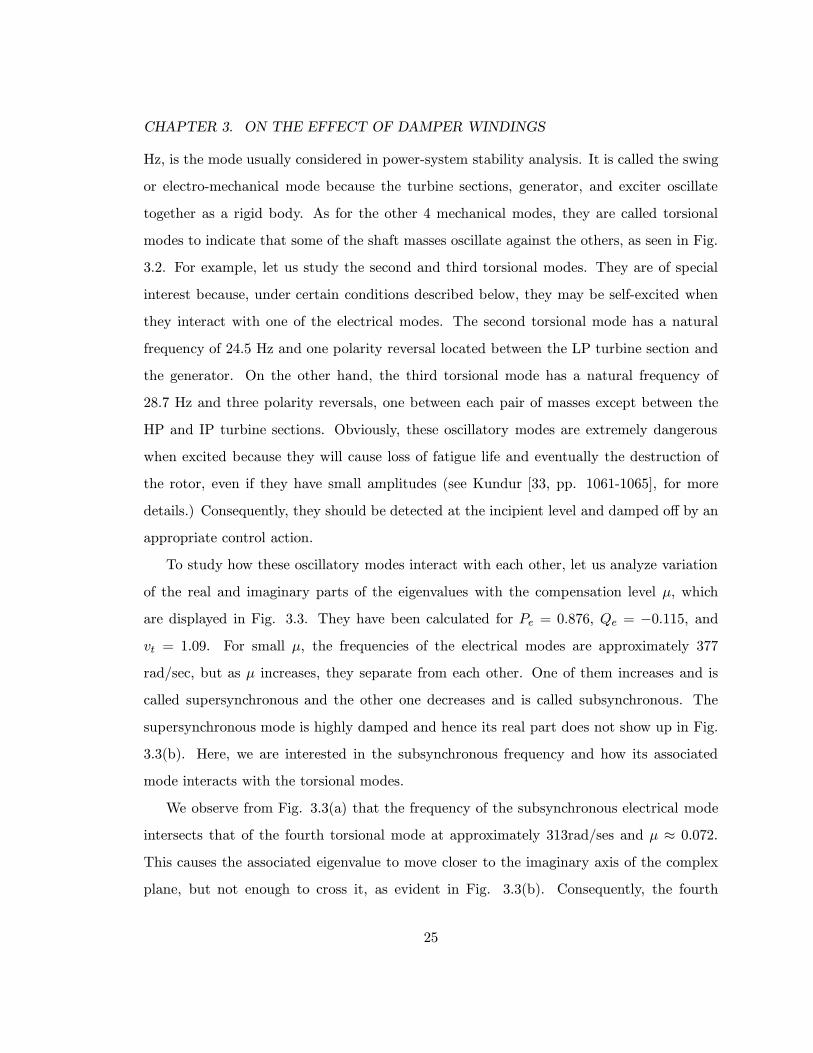
CHAPTER 3. ON THE EFFECT OF DAMPER WINDINGS
Hz, is the mode usually considered in power-system stability analysis. It is called the swing
or electro-mechanical mode because the turbine sections, generator, and exciter oscillate
together as a rigid body. As for the other 4 mechanical modes, they are called torsional
modes to indicate that some of the shaft masses oscillate against the others, as seen in Fig.
3.2. For example, let us study the second and third torsional modes. They are of special
interest because, under certain conditions described below, they may be self-excited when
they interact with one of the electrical modes. The second torsional mode has a natural
frequency of 24.5 Hz and one polarity reversal located between the LP turbine section and
the generator. On the other hand, the third torsional mode has a natural frequency of
28.7 Hz and three polarity reversals, one between each pair of masses except between the
HP and IP turbine sections. Obviously, these oscillatory modes are extremely dangerous
when excited because they will cause loss of fatigue life and eventually the destruction of
the rotor, even if they have small amplitudes (see Kundur [33, pp. 1061-1065], for more
details.) Consequently, they should be detected at the incipient level and damped off by an
appropriate control action.
To study how these oscillatory modes interact with each other, let us analyze variation
of the real and imaginary parts of the eigenvalues with the compensation level µ, which
are displayed in Fig. 3.3. They have been calculated for Pe = 0.876, Qe = −0.115, andvt = 1.09. For small µ, the frequencies of the electrical modes are approximately 377
rad/sec, but as µ increases, they separate from each other. One of them increases and is
called supersynchronous and the other one decreases and is called subsynchronous. The
supersynchronous mode is highly damped and hence its real part does not show up in Fig.
3.3(b). Here, we are interested in the subsynchronous frequency and how its associated
mode interacts with the torsional modes.
We observe from Fig. 3.3(a) that the frequency of the subsynchronous electrical mode
intersects that of the fourth torsional mode at approximately 313rad/ses and µ ≈ 0.072.
This causes the associated eigenvalue to move closer to the imaginary axis of the complex
plane, but not enough to cross it, as evident in Fig. 3.3(b). Consequently, the fourth
25
CHAPTER 3. ON THE EFFECT OF DAMPER WINDINGS
-------------------------------------------------------------------------------
-------------------------------------------------------------------------------
-------------------------------------------------------------------------------
-------------------------------------------------------------------------------
-------------------------------------------------------------------------------
Mode 0
Mode 1
Mode 2
Mode 3
Mode 4(f=49.8 Hz)
(f=12.9 Hz)
(f=24.5 Hz)
(f=28.7 Hz)
(f=2.0 Hz)
Figure 3.2: Mode shapes of the five-mass-turbine-generator system.
26

CHAPTER 3. ON THE EFFECT OF DAMPER WINDINGS
torsional mode does not lose stability. As µ increases further, the frequency of the electrical
mode continues to decrease away from that of the fourth torsional mode while approaching
that of the third torsional mode. The latter is finally crossed at µ ≈ 0.61859. As seen
in Fig. 3.3(b), the eigenvalue of the fourth torsional mode moves to the left, away from
the imaginary axis, until the influence of the electrical mode on the fourth torsional mode
becomes insignificant. On the other hand, the influence of the electrical mode on the
third torsional mode gains sufficient strength to move its eigenvalue transversely across the
imaginary axis into the right-half of the complex plane. The crossing occurs at µ = H1 ≈0.618592, a value termed Hopf bifurcation. There, the third torsional mode loses stability.
This mode regains stability at a reverse Hopf bifurcation, namely µ = H2 ≈ 0.724331, where
the frequencies of both modes start to separate from each other.
As µ passes H2, the frequency of the electrical mode continues its descent toward now
that of the second torsional mode. When the frequency of the electrical mode attains
approximately 154 rad/sec, it intersects that of the second torsional mode at µ ≈ 0.771,
which causes, this time, the eigenvalue of the subsynchronous electrical mode to move to the
right. The interaction between these two modes is strong enough to cause the eigenvalue
of the electrical mode to cross transversely the imaginary axis into the right-half of the
complex plane at a third Hopf bifurcation point, namely µ = H3 ≈ 0.745988. Beyond that
point, the eigenvalue of the electrical mode steadily heads to the right and the power system
never regains stability. It has no stable operating condition.
A synthetic view of the loci of the stable and unstable equilibria in the δr − µ plane
together with the three Hopf bifurcation points is depicted in Fig. 3.4. We observe that the
equilibria are stable and hence all of the modes are positively damped to the left of H1 and
between H2 and H3. The equilibria are unstable between H1 and H2 and beyond H3. For
the H1 −H2 portion of the unstable locus, the second torsional mode is unstable, whereas,
for the portion to the right of H3, the subsynchronous electrical mode is unstable.
Figure 3.5 displays variation of the loci of the Hopf bifurcation points in the Pe−µ plane
for vt = 1.09 and Qe = -0.2. We observe that the first two Hopf bifurcations are insensitive
27
CHAPTER 3. ON THE EFFECT OF DAMPER WINDINGS
0.0 0.4 0.8
0.0
third torsional mode
second torsional mode
first torsional mode
fourth torsional mode
subsynchronous electrical mode
0.0
200.0
fourth torsional mode
subsynchronous electrical mode
third torsional mode
second torsional mode
first torsional mode
R( )λ
Im( )λ
µ
( )a
( )b
Figure 3.3: Variation of the real parts (a) and imaginary parts (b) of the eigenvalues forPe = 0.876, Qe = -0.115, and vt = 1.09. There are three supercritical Hopf bifurcations atµ = H1 ≈ 0.618592, H2 ≈ 0.724331 , and H3 ≈ 0.745988.
28

CHAPTER 3. ON THE EFFECT OF DAMPER WINDINGS
to the value of Pe, whereas the third Hopf bifurcation increases slightly as Pe decreases.
The question that arises here is how these loci vary in the Pe − µ plane as Qe increases
while vt is kept constant at 1.09. We see in Fig. 3.6 that their variations widen the stability
region and move the unstable region to higher values of µ, as expected. We note that all
of the modes are stable to the left of the curve labeled H1 and between the curves labeled
H2 and H3, whereas the second torsional mode and the electrical subsynchronous mode are
unstable between the curves labeled H1 and H2 and to the right of the curve labeled H3,
respectively.
3.2.2 Dynamic Solutions
According to the Hopf bifurcation theorem, the power system possesses small
limit cycles near the Hopf bifurcation points. To investigate the stability of these limit
cycles, we determine the normal forms of the Hopf bifurcations near curves H1,H2, and H3.
To this end, we use the multiple-scales algorithm outlined by Nayfeh and Balachandran [30]
and encoded in MAPLE. It yields the normal form of a Hopf bifurcation for any first-order
system of nonlinear ordinary-differential equations. For the case depicted in Fig. 3.4 for
which Pe = 0.876, Qe = -0.115, and vt = 1.09, variation of the amplitude a of oscillations
with time near a Hopf bifurcation Hi is given by
a′ = (µ−Hi)β1a+ β2a3 (3.48)
In the vicinity of the first Hopf bifurcation H1 ≈ 0.618592, we find that β1 = 25.3281
and β2 = - 0.01339. Because β2 < 0, we conclude that H1 is supercritical and the limit
cycles born as a result of the bifurcation are stable. Their amplitudes are given by
a = 43.4922√µ−H1 (3.49)
Similar results are obtained in the vicinity of the second Hopf bifurcation H2 ≈ 0.618592
with β1 = -3.42 and β2 = - 0.002134, and the third Hopf bifurcation H3 ≈ 0.745988 with
β1 = 290.373 and β2 = -0.412849. Again, because β2 < 0 for both Hopf bifurcations, H2
29

CHAPTER 3. ON THE EFFECT OF DAMPER WINDINGS
0.55 0.60 0.65 0.70 0.75 0.80
1.03
1.04
1.05
1.06
1.07
1.08
H1
H2
H3
SH1
SH2
SH3
µ
δr
Figure 3.4: Bifurcation diagram showing variation of the generator rotor angle δr with thecompensation level µ. The solid lines denote sinks and the dashed lines denote unstablefoci.
30
CHAPTER 3. ON THE EFFECT OF DAMPER WINDINGS
0.60 0.64 0.68 0.72 0.76
0.80
0.90
1.00
Pe
H1
µ
H2
H3
Figure 3.5: Variation of the loci of the Hopf bifurcation points with Pe when vt = 1.09 andQe = −0.2.
31

CHAPTER 3. ON THE EFFECT OF DAMPER WINDINGS
and H3 are supercritical and the created limit cycles are stable with amplitudes given by
a = 40.0328√H2 − µ and a = 26.5205
√µ−H3, respectively.
Let us now study by means of a combination of a two-point boundary-value scheme and
Floquet theory [30] the growth and stability of the limit cycles when µ moves away from
the Hopf bifurcations inside the unstable region. As µ increases from H1, the limit cycle
grows in size while remaining stable with one Floquet multiplier being unity and the 14
remaining Floquet multipliers lying inside the unit circle. See Fig. 3.7(a) for an example
of a limit cycle and Fig. 3.8(a) for the corresponding time history of the generator rotor
angle δr and frequency ωr. The time traces are periodic, the trajectory closes on itself, the
Poincare section consists of a single point, and the FFT consists of a single frequency and
its harmonics.
When µ passes the critical value SH1 ≈ 0.63848, two of the Floquet multipliers exit the
unit circle away from the real axis, signifying that SH1 is a secondary Hopf bifurcation.
There, the limit cycle loses stability and gives way to a two-period quasiperiodic (two-torus)
attractor. Two examples are displayed in Figs. 3.7(b) and (c). The corresponding time
histories are given in Fig. 3.8(b) and (c). The time traces are modulated, the trajectories
do not close on themselves, the Poincare sections consist of closed curves, and the FFTs
consist of two incommensurate frequencies, their multiples, and combinations.
As µ increases slightly above SH1 to C1 ≈ 0.63868, the two-torus collides with its
basin boundary, yielding their destruction in a bluesky catastrophe. This can be observed
in Fig. 3.9, which displays the time histories of δr and ωr in the vicinity of the bluesky
catastrophe. We note that, when the basin of attraction disappears at C1, the generator
angle δr steadily decreases from 19 to settle for a while at −548 and move again to another
value, and so forth, indicating that the generator is unable to regain synchronism. Similar
results are obtained when µ decreases below SH2 ≈ 0.70193 to C2 ≈ 0.70015 or increases
beyond SH3 ≈ 0.75799 to C3 ≈ 0.76505. Again, at C2 and C3, there are no stable operating
conditions.
32

CHAPTER 3. ON THE EFFECT OF DAMPER WINDINGS
0.60 0.65 0.70 0.75 0.80
0.80
1.00H
1H
2H
3
µ
Pe
Figure 3.6: The influence of varying Qe on the locations of the Hopf bifurcations in thePe − µ plane for vt = 1.09. The solid lines correspond to Qe = 0.45, the dashed linescorrespond to Qe = 0.15, and the dashed-dotted lines correspond to Qe = −0.2.
33
CHAPTER 3. ON THE EFFECT OF DAMPER WINDINGS
ω r
ω r
ω r
δr δr frequency
Figure 3.7: Two-dimensional projections of the phase portrait (left) and the Poincare section(middle) onto the ωr − δr plane and the FFT of the corresponding quadrature-axis voltageecq across the capacitor (right) for µ = (a) 0.63840, (b) 0.63848, and (c) 0.63867. Thesolution at (a) is a limit cycle, at (b) is a two-torus attractor recorded well before thebluesky catastrophe, and at (c) is a two-torus attractor located just before it disappears ina bluesky catastrophe.
34

CHAPTER 3. ON THE EFFECT OF DAMPER WINDINGS
ωr
ωr
ω r
δr
δr
δr
0 20.88
1.11
0.88
1.11
0.88
1.11
0 20.00
1.18
0.00
1.18
0.00
1.18
time time
Figure 3.8: Time traces of the generator rotor angle δr and frequency ωr at µ = (a) 0.63840,(b) 0.63848, and (c) 0.63867.
35

CHAPTER 3. ON THE EFFECT OF DAMPER WINDINGS
ωr
(a)
(b)
0.3
1.5
0 40
-550
20
δr
time
Figure 3.9: Time histories of the generator rotor speed ωr (in rad/sec) and angle δr (inrad) at µ = 0.63868, which is slightly larger than µ = C1 ≈ 0.63867 at which the blueskycatastrophe occurs.
36
CHAPTER 3. ON THE EFFECT OF DAMPER WINDINGS
3.3 Effect of Damper Windings
Although damper windings have some benefits in transient stability, such as damping
off speed oscillations, they may induce subsynchronous resonance. Hamdan [67] used linear
theory to analyze SSR in a single-machine-infinite-busbar power system. He showed that
damper windings reduce the compensation level at which subsynchronous resonance occurs.
In this section, we study the effect of placing damper windings on either the q-axis, or the d-
axis, or both axes on subsynchronous resonance. We evaluate the influence of these damper
windings on the Hopf bifurcations and their types and the ensuing dynamic responses.
3.3.1 Q-Axis Damper Windings
For XQ = 1.695,Xmq = 1.58, and RQ = 0.006, we show in Fig. 3.10 variation
of the real and imaginary parts of the eigenvalues with µ. The Jacobian matrix of the
system has 14 complex conjugate eigenvalues and two real eigenvalues. As in the case
without damper windings, there are 7 oscillatory modes, two associated with the electrical
subsystem and 5 associated with the mechanical system. The two real eigenvalues are
negative, one of them is associated with the field windings and the other is associated
with the damper windings. As in the case of no damper windings, as µ increases, one of
the electrical frequencies (supersynchronous) increases, whereas the other (subsynchronous)
decreases. Comparing Figs. 3.4 and 3.10, we note that the damper windings accelerate the
decrease in the subsynchronous electrical frequency.
As µ increases further, the frequency of the electrical mode intersects those of the fourth,
third, second, and first torsional modes for values of µ < 1.0, resulting in four interaction
regions. As in the case without damper windings, the interaction of the electrical and
fourth torsional modes is not strong enough to overcome their dampings and, hence, the
equilibrium solution retains its stability. However, the other three interactions are strong
enough to overcome the dampings of the interacting modes and produce three unstable
intervals. In contrast with the case without damper windings where the unstable intervals do
37

CHAPTER 3. ON THE EFFECT OF DAMPER WINDINGS
not overlap, the unstable intervals overlap in this case, resulting in a single unstable region.
Therefore, once the equilibrium solution loses its stability due to the second interaction,
it does not regain it for any larger value of µ, implying the existence of only one Hopf
bifurcation point.
Comparing Figs. 3.4 and 3.10, we conclude that the damper windings on the q-axis
have a destabilizing influnace on the power system. First, they decrease the value of µ at
which the first Hopf bifurcation occurs from 0.6186 to 0.4222. Second, they eliminate the
stable region 0.7243 ≤ µ ≤ 0.7460.
In Fig. 3.11, we show variation of the real and imaginary parts of the eigenvalues when
RQ is increased to 0.015. These results are qualitatively similar to those obtained in Fig.
3.10 for RQ = 0.006. However, the rates of growth of the unstable modes have increased by
more than 100%. This increase may be attributed to the induction effect. In Fig. 3.12, we
show variation of the maxima of the real parts of the eigenvalues with RQ for selected values
of µ. For a given value of µ, the growth rate of the instability increases as RQ increases,
attains a maximum, and then decreases.
When RQ ≈ 0, it follows from Eq. (3.30) that iQ ≈ iqXmq/XQ+ constant, which,
when substituted into Eqs. (3.27) and (3.28), leads to an effective inductance Xqe given by
Xqe ≈ Xq −X2mq/XQ. Replacing Xq by Xqe in Eqs. (3.15)-(3.29) and putting iQ = iD = 0
(no damper windings), we find that the Hopf bifurcation occurs very close to that obtained
by using Eqs. (3.15)-(3.30) with the q-axis damper windings.
Again, to detremine whether the created limit cycles due to the Hopf bifurcation are
stable or unstable, we implement the multiple-scales algorithm outlined by Nayfeh and
Balachandran [29] by using MAPLE to reduce the dynamical power system to its normal
form, Eq. (3.48), in the vicinity of the Hopf bifurcation point µ = H ≈ 0.422172. For
Pe = 0.876, Qe = −0.115, and vt = 1.09, we find that β1 = 7.41447 and β2 = 0.0004867.
Thus, the Hopf bifurcation H ≈ 0.422172 is subcritical and the limit cycles born as a result
of the bifurcation are unstable. Their amplitudes are given by
38

CHAPTER 3. ON THE EFFECT OF DAMPER WINDINGS
a = 123.426√µ−H (3.50)
The dynamics of the system near the subcritical Hopf bifurcation H of Fig. 3.13 is much
more complicated than the dynamics of the system near the supercritical Hopf bifurcations
in the previous section. Locally, the system possesses a stable equilibrium solution and a
small unstable limit cycle for values of µ slightly below that corresponding to H. As µ
increases past H, the equilibrium solution loses stability and the small unstable limit cycle
disappears. As µ is decreased below H, the unstable limit cycle deforms and increases in
size until the branch of unstable limit cycles meets a branch of stable large-amplitude limit
cycles at µ = 0.406425, corresponding to point CF . As µ is decreased further, the stable
and unstable limit cycles collide and annihilate each other in a cyclic-fold bifurcation.
We again use a combination of a two-point boundary-value scheme and Floquet theory
[30] to study the growth and stability of the large-amplitude limit cycles when µ increases
from CF . As µ increases from CF , the stable limit cycle grows in size while remaining
stable with one Floquet multiplier being unity and the 15 remaining Floquet multipliers
lying inside the unit circle. In Fig. 3.14(a) we show an example of a limit cycle. The phase
portrait is a closed curve, the time trace of δr is periodic, and the FFT of δr consists of a
single frequency and its harmonics.
When µ increases beyond a critical value SH ≈ 0.411385, two Floquet multipliers exit
the unit circle away from the real axis, signifying that SH is a secondary Hopf bifurcation.
There, the limit cycle loses stability and gives way to a two-period quasiperiodic (two-torus)
attractor. Two examples are displayed in Figs. 3.14(b) and (c). The trajectories do not
close on themselves, the FFTs consist of two incommensurate frequencies, their multiples,
and combinations, and the time traces are modulated.
As µ increases slightly above SH to C ≈ 0.418574, the two-torus collides with its basin
boundary, resulting in their destruction in a bluesky catastrophe. This can be observed in
Fig. 3.15, which displays the time histories of δr and ωr at µ = 0.418576, which is slightly
larger than C ≈ 0.418574. We note that the bluesky catastrophe and hence the system
39
CHAPTER 3. ON THE EFFECT OF DAMPER WINDINGS
loses synchronism at a value of µ that is less than H.
3.3.2 D-Axis Damper Windings
For XD = 1.666,Xmd = 1.66, and RD = 0.0037, we show in Fig. 3.16 variation
of the real and imaginary parts of the eigenvalues with µ. Comparing Figs. 3.16 and 3.3,
we note that the d-axis damper windings accelerate the decrease of the subsynchronous
electrical frequency and hence its interaction with those of the fourth, third, and second
torsional modes, as in the case of the q-axis damper windings. Consequently, the d-axis
damper windings reduce the compensation level at which the Hopf bifurcation occurs from
µ ≈ 0.6186 to µ ≈ 0.5628 . Again, the instability regions overlap and there is only one Hopf
bifurcation; that is, the d-axis damper windings eleminate the stable region 0.7243 ≤ µ ≤0.7466.
Next, we investigate the dynamics of the power system near the Hopf bifurcation H ≈0.5628 by determining its normal form, Eq. (3.48). For the case depicted in Fig. 3.17,
Pe = 0.876, Qe = -0.115, and vt = 1.09, we find that β1 = 9.0094 and β2 = - 0.00898363.
Because β2 < 0, we conclude that H is supercritical and the limit cycles born as a result of
the bifurcation are stable. Their amplitudes are given by
a = 31.653√µ−H (3.51)
To study the development and stability of the limit cycles when µ moves away from the
Hopf bifurcation inside the unstable region, we use a combination of a two-point boundary-
value algorithm and Floquet theory. As µ increases from H, the limit cycle grows in size
while remaining stable with one Floquet multiplier being unity and the 15 remaining Floquet
multipliers lying inside the unit circle. See Fig. 3.18(a) for an example of a limit cycle. The
time trace is periodic, the FFT of the corresponding generator rotor angle δr consists of a
discrete frequency and its harmonics, and the trajectory closes on itself.
When µ passes a critical value SH ≈ 0.59283, two of the Floquet multipliers exit the
unit circle away from the real axis, signifying that SH is a secondary Hopf bifurcation.
40
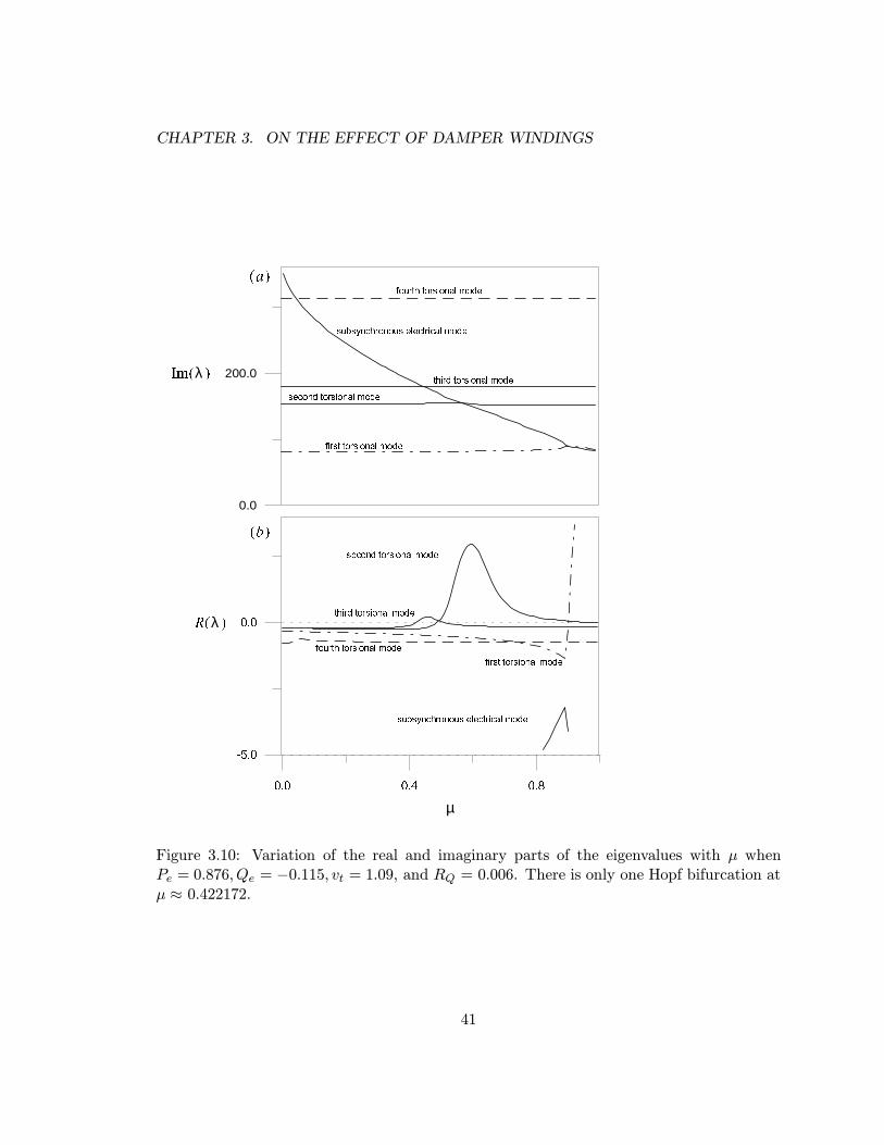
CHAPTER 3. ON THE EFFECT OF DAMPER WINDINGS
0.0 0.4 0.8
-5.0
0.0
second torsional mode
third torsional mode
fourth torsional mode
first torsional mode
subsynchronous electrical mode
0.0
200.0
fourth torsional mode
subsynchronous electrical mode
third torsional mode
second torsional mode
first torsional mode
( )a
( )b
R( )λ
Im( )λ
µ
Figure 3.10: Variation of the real and imaginary parts of the eigenvalues with µ whenPe = 0.876, Qe = −0.115, vt = 1.09, and RQ = 0.006. There is only one Hopf bifurcation atµ ≈ 0.422172.
41
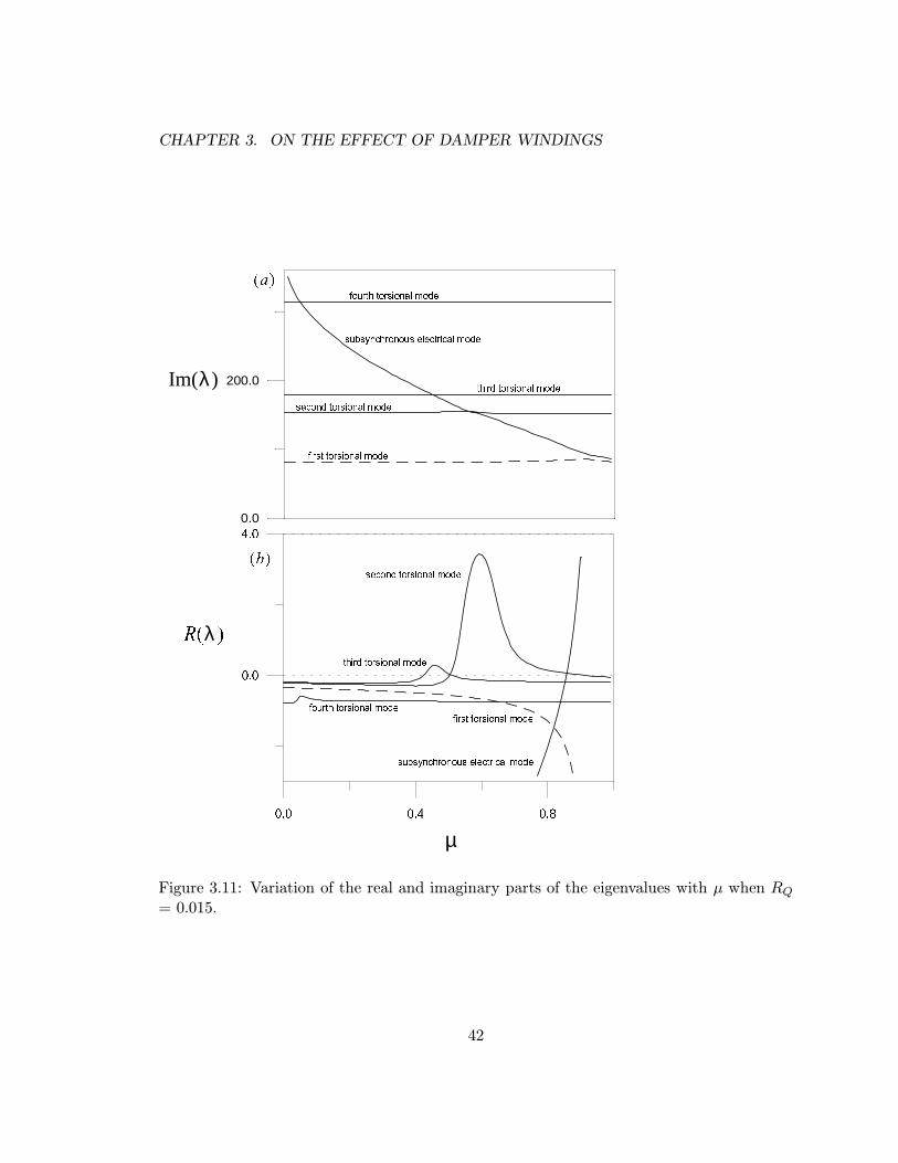
CHAPTER 3. ON THE EFFECT OF DAMPER WINDINGS
0.0 0.4 0.8
0.0
4.0
second torsional mode
third torsional mode
fourth torsional mode
first torsional mode
subsynchronous electrical mode
0.0
200.0
fourth torsional mode
subsynchronous electrical mode
third torsional mode
second torsional mode
first torsional mode
Im( )λ
µ
( )a
( )b
R( )λ
Figure 3.11: Variation of the real and imaginary parts of the eigenvalues with µ when RQ
= 0.015.
42

CHAPTER 3. ON THE EFFECT OF DAMPER WINDINGS
0.00 0.01 0.02
-0.02
-0.01
0.00
0.01
R( )λ
RQ
µ1
µ2
µ3
Figure 3.12: Variation of the maximum real parts of the eigenvalues with RQ for threevalues of µ : µ1 = 0.422127, µ2 = 0.422027, and µ3 = 0.421027.
43

CHAPTER 3. ON THE EFFECT OF DAMPER WINDINGS
0.0 0.4 0.8
-2.2
-2.1
-2.0
-1.9
δ r
µ
HSH
H
SH
CF
Figure 3.13: Bifurcation diagram showing variation of the generator rotor angle δr with thecompensation level µ. The solid line denotes sinks and the dashed line denotes unstablefoci.
44
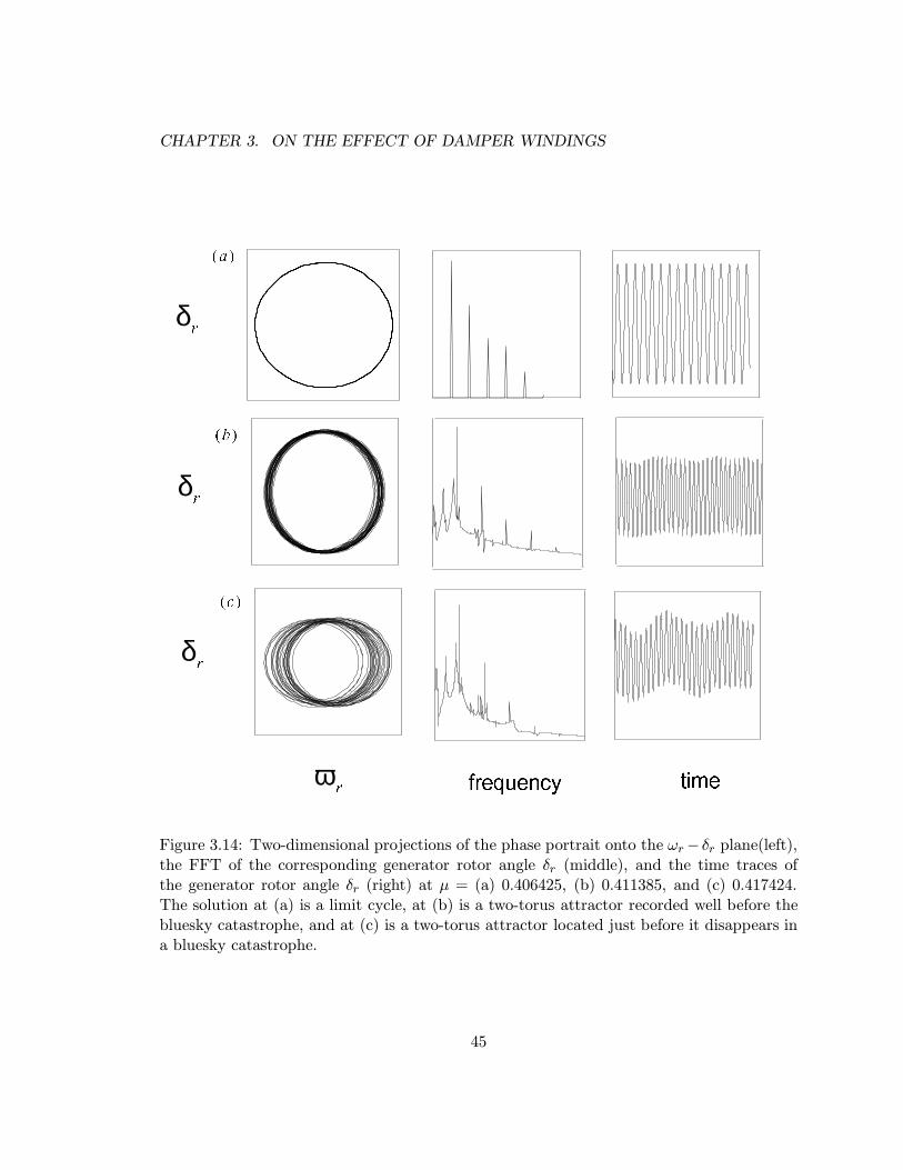
CHAPTER 3. ON THE EFFECT OF DAMPER WINDINGS
( )a
( )b
( )c
frequency time
δr
δr
δr
ωr
Figure 3.14: Two-dimensional projections of the phase portrait onto the ωr− δr plane(left),the FFT of the corresponding generator rotor angle δr (middle), and the time traces ofthe generator rotor angle δr (right) at µ = (a) 0.406425, (b) 0.411385, and (c) 0.417424.The solution at (a) is a limit cycle, at (b) is a two-torus attractor recorded well before thebluesky catastrophe, and at (c) is a two-torus attractor located just before it disappears ina bluesky catastrophe.
45

CHAPTER 3. ON THE EFFECT OF DAMPER WINDINGS
0.0
0.0 20.0 40.0
-40.0
0.0
( )a
( )b
ωr
δr
time
Figure 3.15: Time histories of the generator rotor speed ωr (in rad/sec) and angle δr (inrad) at µ = 0.418576, which is slightly larger than C ≈ 0.418574 at which the blueskycatastrophe that occurs.
46

CHAPTER 3. ON THE EFFECT OF DAMPER WINDINGS
0.0 0.4 0.8
0.0
0.0
400.0
supersynchronous electric mode
subsynchronous electric mode
fourth torsional mode
third torsional mode
second torsional mode
first torsional mode
swing mode
second torsional mode
third torional mode
swing mode
fourth torsional modefirst torsional mode
subsynchronous electric mode
supersynchronous electric mode
( )b
( )a
µ
R( )λ
Im( )λ
Figure 3.16: Variation of the real and imaginary parts of the eigenvalues with µ in the caseof d-axis damper windings when RD= 0.0037.
47

CHAPTER 3. ON THE EFFECT OF DAMPER WINDINGS
0.0 0.4 0.8
1.0
1.2
δ r
µ
SHH
Figure 3.17: Bifurcation diagram showing variation of the generator rotor angle δr with thecompensation level µ. The solid line denotes sinks and the dashed line denotes unstablefoci.
48

CHAPTER 3. ON THE EFFECT OF DAMPER WINDINGS
There, the limit cycle loses stability and gives way to a two-period quasiperiodic (two-
torus) attractor. Two examples are displayed in Figs. 3.18(b) and (c). The time histories
are modulated, the trajectories do not close on themselves, and the FFTs of δr seem to
consist of two incommensurate frequencies, their multiples, and combinations.
As µ increases slightly above SH to C ≈ 0.6298, the two-torus collides with its basin
boundary, yielding their destruction in a bluesky catastrophe. This can be observed in Fig.
3.19, which displays the time history of δr in the vicinity of the bluesky catastrophe.
3.3.3 Q and D - Axes Damper Windings
For XQ = 1.696,Xmq = 1.58, RQ = 0.006,XD = 1.666,Xmd = 1.66, and RD = 0.0037,
we show in Fig. 3.20 variation of the real and imaginary parts of the eigenvalues with µ.
Again, we note that the two damper windings accelerate the decrease in the subsynchronous
electrical frequency. The unstable regions overlap so that there is only one Hopf bifurcation
point. Moveover, the Hopf bifurcation point is reduced to 0.4004. In Fig. 3.21, we show
the influence of the damper windings on the loci of the Hopf bifurcation in the Pe−µ plane
for vt = 1.09 and Qe = −0.115. Clearly, placing damper windings on either the d-axis or
the q-axis or both axes reduces the compensation level at which the Hopf bifurcations and
hence the instability of the power system occur. So, we conclude that including damper
windings along either the q-axis, the d-axis, or both axes shrinks the stable region of the
power system, in agreement with Hamdan [67]. Moreover, the q-axis damper windings are
more destabilizing than the d-axis damper windings.
Now we investigate the dynamics of the power system in the vicinity of the Hopf bifur-
cation H ≈ 0.400411 by determining its normal form, Eq. (3.48). For the case depicted in
Fig. 3.22, Pe = 0.876, Qe = -0.115, and vt = 1.09, we find that β1 = 5.77715 and β2 = -
0.000211097. Because β2 < 0, we conclude that H is supercritical and the limit cycles born
as a result of the bifurcation are stable. Their amplitudes are given by
a = 165.4305√µ−H (3.52)
49

CHAPTER 3. ON THE EFFECT OF DAMPER WINDINGS
δr
δr
δr
ωr
(a)
( )b
( )c
Figure 3.18: Two-dimensional projections of the phase portrait onto the ωr− δr plane(left),the FFT of the corresponding generator rotor angle δr (middle), and the time traces ofthe generator rotor angle δr (right) at µ = (a) 0.5738, (b) 0.59295, and (c) 0.59585. Thesolution at (a) is a limit cycle, at (b) is a two-torus attractor recorded well before thebluesky catastrophe, and at (c) is a two-torus attractor located just before it disappears ina bluesky catastrophe.
50

CHAPTER 3. ON THE EFFECT OF DAMPER WINDINGS
0.0 4.0
-40.0
0.0
δr
time
Figure 3.19: The time history of the generator rotor angle δr (in rad) at µ = 0.60787, whichis slightly larger than C ≈ 0.60785 at which the bluesky catastrophe that occurs.
51

CHAPTER 3. ON THE EFFECT OF DAMPER WINDINGS
0.0 0.4 0.8
0.0
Im( )λ
R( )λ
µ
0.0
400.0
( )a
( )b
Figure 3.20: Variation of the real and imaginary parts of the eigenvalues with µ in the caseof d-and-q axes damper windings when RQ = 0.006 and RD = 0.0037.
52

CHAPTER 3. ON THE EFFECT OF DAMPER WINDINGS
0.4 0.6
0.4
0.8
Pe
µ
b c da
Figure 3.21: Variation of the loci of the Hopf bifurcation points with Pe when vt = 1.09 andQe = −0.115. Line a corresponds to RD = RQ = 0.0037, line b corresponds to RQ = 0.0037and RD = 0.0, line c corresponds to RD = 0.0037 and RQ = 0.0, and line d corresponds toRD = RQ = 0.0.
53

CHAPTER 3. ON THE EFFECT OF DAMPER WINDINGS
δ r
µ
SHH
Figure 3.22: Bifurcation diagram showing variation of the generator rotor angle δr with thecompensation level µ. The solid line denotes sinks and the dashed line denotes unstablefoci.
54

CHAPTER 3. ON THE EFFECT OF DAMPER WINDINGS
Next, we study the growth and stability of the limit cycles when µ moves away from
the Hopf bifurcation inside the unstable region by means of a two-point boundary-value
algorithm and Floquet theory [30]. As µ increases from H, the limit cycle grows in size
while remaining stable with one Floquet multiplier being unity and the 16 remaining Floquet
multipliers lying inside the unit circle. See Figs. 3.23(a) for an example of a limit cycle and
the corresponding time trace of the generator rotor angle δr. The time history is uniform,
the FFT consists of a single frequency and its harmonic, and the trajectory closes on itself.
When µ passes a critical value SH ≈ 0.40271, two of the Floquet multipliers exit the
unit circle away from the real axis, signifying that SH is a secondary Hopf bifurcation.
There, the limit cycle loses stability and gives way to a two-period quasiperiodic (two-
torus) attractor. Two examples are displayed in Figs. 3.23(b) and (c). The time traces
are modulated, the FFTs consist of two incommensurate frequencies, their multiples and
their combinations, and the trajectories do not close on themselves. As µ increases slightly
above SH to C ≈ 0.40641, the two-torus collides with its basin boundary, yielding their
destruction in a bluesky catastrophe.
55
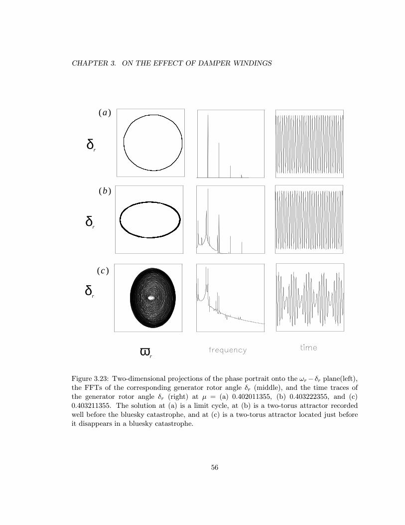
CHAPTER 3. ON THE EFFECT OF DAMPER WINDINGS
( )a
( )b
( )c
δr
δr
δ r
ω r
Figure 3.23: Two-dimensional projections of the phase portrait onto the ωr− δr plane(left),the FFTs of the corresponding generator rotor angle δr (middle), and the time traces ofthe generator rotor angle δr (right) at µ = (a) 0.402011355, (b) 0.403222355, and (c)0.403211355. The solution at (a) is a limit cycle, at (b) is a two-torus attractor recordedwell before the bluesky catastrophe, and at (c) is a two-torus attractor located just beforeit disappears in a bluesky catastrophe.
56

Chapter 4
ON THE EFFECT OF MACHINE SATURATION
To make the bifurcation analysis of subsynchronous resonance of power systems
simple and manageable, all of the authers have neglected the effect of stator and rotor
iron saturation in synchronous machines. However, the importance of saturation has been
recognized by many authors [e.g, 34,35,...,57]. In this chapter, we carry out a bifurcation
analysis in a complete model of the CHOLLA#4 station. The model includes saturation, but
neglects the dynamics of the automatic voltage regulator (AVR) and the turbine governor.
It is evident that accounting for saturation in both the d- and q-axes can lead to an
improvement in the accuracy of the simulation models. To account for the iron saturation
in stability studies, one usually makes the following assumptions[33]:
(i) The leakage fluxes are in air for a large portion of their pathes. Hence, they are not
significantly affected by saturation of the iron core. So, the leakage inductances are
independent of the iron saturation. As a result, the only elements that saturate are
the mutual flux linkages ψmd and ψmq.
(ii) The leakage fluxes are usually small and their pathes coincide with that of the main
flux for only a small part of its path. So, saturation can be determined by the air-gap
flux linkage only.
(iii) The saturation relationship between the resultant air-gap flux and the mmf under
loaded conditions is the same as that under no-load conditions. This allows the
saturation characteristics to be represented by the open-circuit saturation curve.
In this chapter, we use the modern methods of nonlinear dynamics to analyze the effect of
machine saturation on subsynchronous resonance of another practical power system model.
57

CHAPTER 4. ON THE EFFECT OF MACHINE SATURATION
AAAAAAAAAAAAAAAAAAAAAAAAAAAAAAAAAAAAAAAA
AAAAAAAAAAAAAAAAAAAAAAAAAAAAAAAAAAAAAAAA
AAAAAAAAAAAAAAAAAAAAAAAAAAAAAA
AAAAAAAAAAAAAAAAAAAAAAAAAAAAAAAAAAAAAAAA
AAAAAAAAAAAAAAAAAAAAAAAAAAAAAAAAAAAAAAAA
AAAAAAAAAAAAAAAAAAAAAAAAAAAAAA
AAAAAAAAAAAAAAAAAAAAAAAAAAAAAAAAAAAAAAAA
AAAAAAAAAAAAAAAAAAAAAAAAAAAAAAAAAAAAAAAA
AAAAAAAAAAAAAAAAAAAAAAAAAAAAAA
AAAAAAAAAAAAAAAAAAAAAAAAAAAAAAAAAAAAAAAA
AAAAAAAAAAAAAAAAAAAAAAAAAAAAAAAAAAAAAAAA
AAAAAAAAAAAAAAAAAAAAAAAAAAAAAA
AAAAAAAAAAAAAAAAAAAA
AAAAAAAAAAAAAAAAAAAA
AAAAA
AAAAAAAAAAAAAAAAAAAAAAAAAAAAAAAAAAAAAAAA
AAAAAAAAAAAAAAAAAAAAAAAAAAAAAAAAAAAAAAAA
AAAAAAAAAAAAAAAAAAAA
HP CHL LP CLG Gen
Rl XlXc
Vo
Figure 4.1: A schematic diagram for a series capacitor-compensated single-machine powersystem. The mechanical system consists of a high-pressure (HP), a coupling mass (CHL),a low-pressure (LP), and a coupling mass (CLG) turbine section, and a generator (Gen).
In Sec. 4.1, we briefly describe the CHOLLA#4 generator, in Sec. 4.2, we analyze the case
of no saturation, and in Sec. 4.3, we analyze the effect of saturation on subsynchronous
resonance of the power system.
4.1 System Description
We consider a single-machine-infinite-busbar (SMIB) power system, as shown in Fig. 4.1.
The model and its parameters are chosen to represent the characteristics of the CHOLLA#4
generator with respect to the SOWARO station at the Arizona Public Service when the
generator is heavily loaded.
To obtain analytical formulas for the fluxes ψmd and ψmq as functions of the currents,
we represent the test data which discussed by Denndon in [52], shown in Fig. 4.2, by the
following third-order polynomials:
58
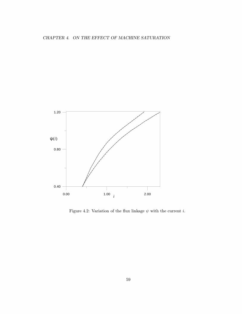
CHAPTER 4. ON THE EFFECT OF MACHINE SATURATION
0.00 1.00 2.00
0.40
0.80
1.20
ψ( )i
i
Figure 4.2: Variation of the flux linkage ψ with the current i.
59
CHAPTER 4. ON THE EFFECT OF MACHINE SATURATION
ψmd = d0 + d1(if − id) + d2(if − id)2 + d3(if − id)
3 (4.1)
ψmq = q0 + q1(iQ − iq) + q2(iQ − iq)2 + q3(iQ − iq)
3 (4.2)
where the dn and qn are constants. Clearly, the mutual flux linkages ψmd and ψmq are
nonlinear functions of the machine currents id, iq, if , and iQ. The d-and q-axes flux linkages
ψd and ψq can be determined from the mutual flux linkages ψmd and ψmq as follows:
ψd = ψmd −Xleid (4.3)
ψq = ψmq −Xleiq (4.4)
ψf = ψmd +Xleif (4.5)
ψQ = ψmq +XleiQ (4.6)
where Xle is the leakage reactance.
The power-system model is governed by 16 first-order nonlinear ordinary-differential
equations, 6 of them represent the electrical subsystem while the other 10 represent the
mechanical subsystem. The mechanical subsystem consists of a high-pressure (HP) and a
low-pressure (LP) turbine section, a generator, and two coupling masses. One couples the
high and low-pressure turbines and the second couples the low-pressure turbine with the
generator, as indicated in Fig. 4.1.
In this formulation, the dynamics of the automatic voltage regular (AVR) and the
turbine governor are neglected. The dynamics of the damper windings on the q-axis as
well as the machine saturation are included. Substituting Eqs. (4.1)-(4.6) into Eqs. (3.1)-
(3.29), one obtains the following equations:
60
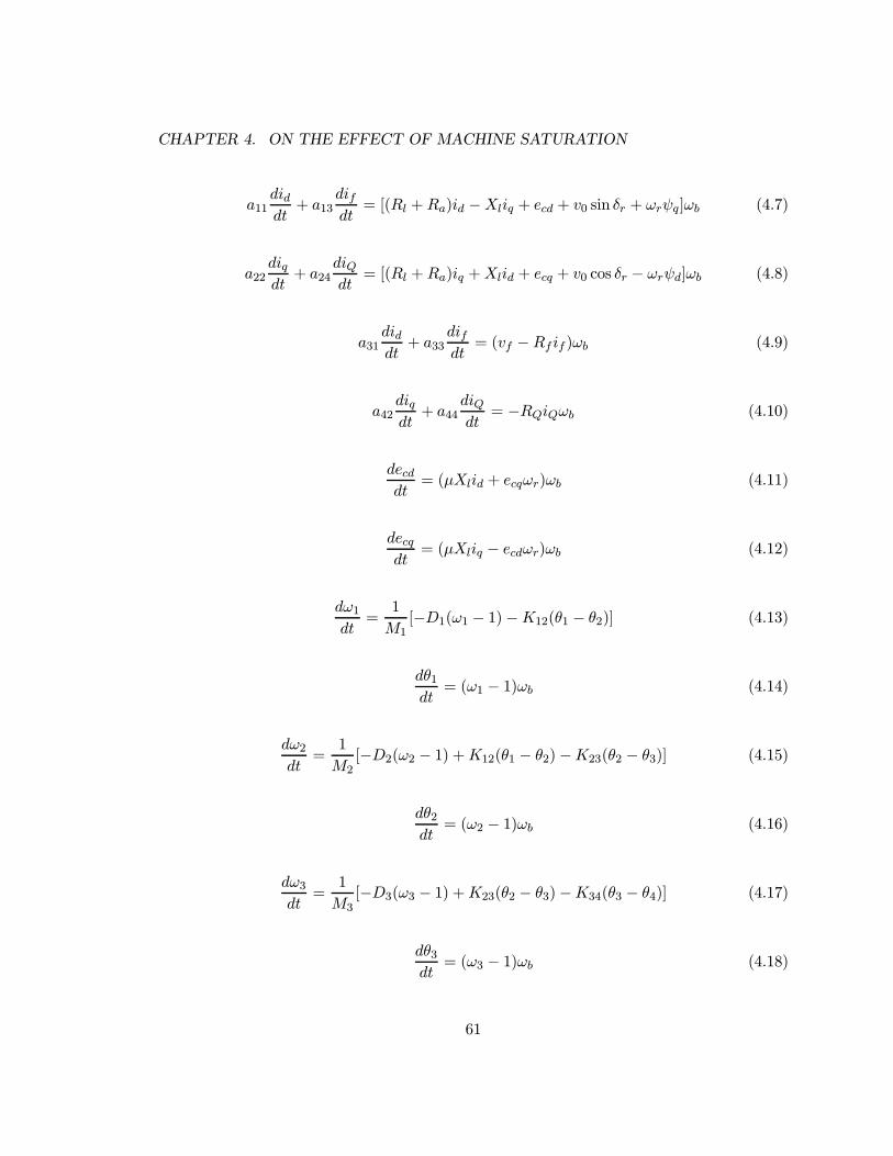
CHAPTER 4. ON THE EFFECT OF MACHINE SATURATION
a11diddt
+ a13difdt
= [(Rl +Ra)id −Xliq + ecd + v0 sin δr + ωrψq]ωb (4.7)
a22diqdt
+ a24diQdt
= [(Rl +Ra)iq +Xlid + ecq + v0 cos δr − ωrψd]ωb (4.8)
a31diddt
+ a33difdt
= (vf −Rf if )ωb (4.9)
a42diqdt
+ a44diQdt
= −RQiQωb (4.10)
decddt
= (µXlid + ecqωr)ωb (4.11)
decqdt
= (µXliq − ecdωr)ωb (4.12)
dω1dt
=1
M1[−D1(ω1 − 1)−K12(θ1 − θ2)] (4.13)
dθ1dt
= (ω1 − 1)ωb (4.14)
dω2dt
=1
M2[−D2(ω2 − 1) +K12(θ1 − θ2)−K23(θ2 − θ3)] (4.15)
dθ2dt
= (ω2 − 1)ωb (4.16)
dω3dt
=1
M3[−D3(ω3 − 1) +K23(θ2 − θ3)−K34(θ3 − θ4)] (4.17)
dθ3dt
= (ω3 − 1)ωb (4.18)
61

CHAPTER 4. ON THE EFFECT OF MACHINE SATURATION
dω4dt
=1
M4[−D4(ω4 − 1) +K34(θ3 − θ4)−K45(θ4 − δr)] (4.19)
dθ4dt
= (ω4 − 1)ωb (4.20)
dωrdt
=1
M5[−D5(ωr − 1) +K45(θ4 − δr) + Tm − Te] (4.21)
dδrdt
= (ωr − 1)ωb (4.22)
where
µ = Xc/Xl,
Te = iqψd − idψq,
a11 = −ζ1 −Xl −Xle,
a22 = −ζ2 −Xl −Xle,
a33 = ζ1 +Xlf ,
a44 = ζ2 +XlQ,
a13 = −a31 = ζ1,
a24 = −a42 = ζ2,
where
ζ1 = d1 + 2d2(if − id) + 3d3(if − id)2,
ζ2 = q1 + 2q2(iQ − iq) + 3q3(iQ − iq)2
Here Xle, Xlf , and XlQ are the leakage reactances.
Equations (4.7)-(4.22) constitute a system of 16 first-order nonlinear ordinary-differential
equations describing the dynamics of the SMIB power system shown in Fig. 4.1. The 16
62

CHAPTER 4. ON THE EFFECT OF MACHINE SATURATION
state variables of the system are id, iq, if , iQ, ecd, ecq, ω1, θ1, ω2, θ2, ω3, θ3, ω4, θ4, ωr, and δr.
The parameters used in this study in p.u. for the generator and the line are
Rf = 0.001252, Ra = 0.0045, X` = 0.08366, R` = 0.00172,
RQ = 0.009957, Xle = 0.1450, Xlf = 0.1061, XlQ = 0.3819,
d0 = −0.1626, d1 = 1.7374, d2 = −0.8939, d3 = 0.1876,
q0 = 0.0635, q1 = 0.9808, q2 = −0.3244, q3 = 0.0489
The mechanical damping coefficients and the inertias and stiffnesses in p.u. are
D1 = 0.02677, M1 = 0.4930,
D2 = 0.0, M2 = 0.03107, K12 = 107.611,
D3 = 0.04150, M3 = 2.8383, K23 = 61.705,
D4 = 0.0, M4 = 0.1156, K34 = 141.413,
D5 = 0.06832, M5 = 1.6512, K45 = 175.208.
4.2 The Case of No Saturation
In the case of no saturation, we set d0, d2, d3, q0, q2, and q3 equal to zero in Eqs.
(4.1) and (4.2) and obtain a system of 16 ordinary-differential equations. The operating
conditions are obtained from the system of equations by setting the derivatives of the state
variables of the system (4.7)-(4.22) equal to zero. The result is summarized in Appendix A.
When Pe = 0.9, Qe = 0.4358, and vt = 1.0, we show variation of the real and imaginary
parts of the eigenvalues with µ in Fig. 4.3. There are 14 complex and two real eigenval-
ues. Because the Jacobian matrix is real, the complex conjugate of each complex value
is an eigenvalue, yielding 7 oscillatory modes. Two modes are electrical modes and 5 are
mechanical modes. The mode with the lowest frequency is the swing or electro-mechanical
mode whereas the other four mechanical modes are torsional modes. Two of the torsional
modes, the third and the fourth modes, are damped and have very high frequencies, namely,
1030 and 1450 rad/sec. Hence, they do not interact with the electrical modes for realistic
63
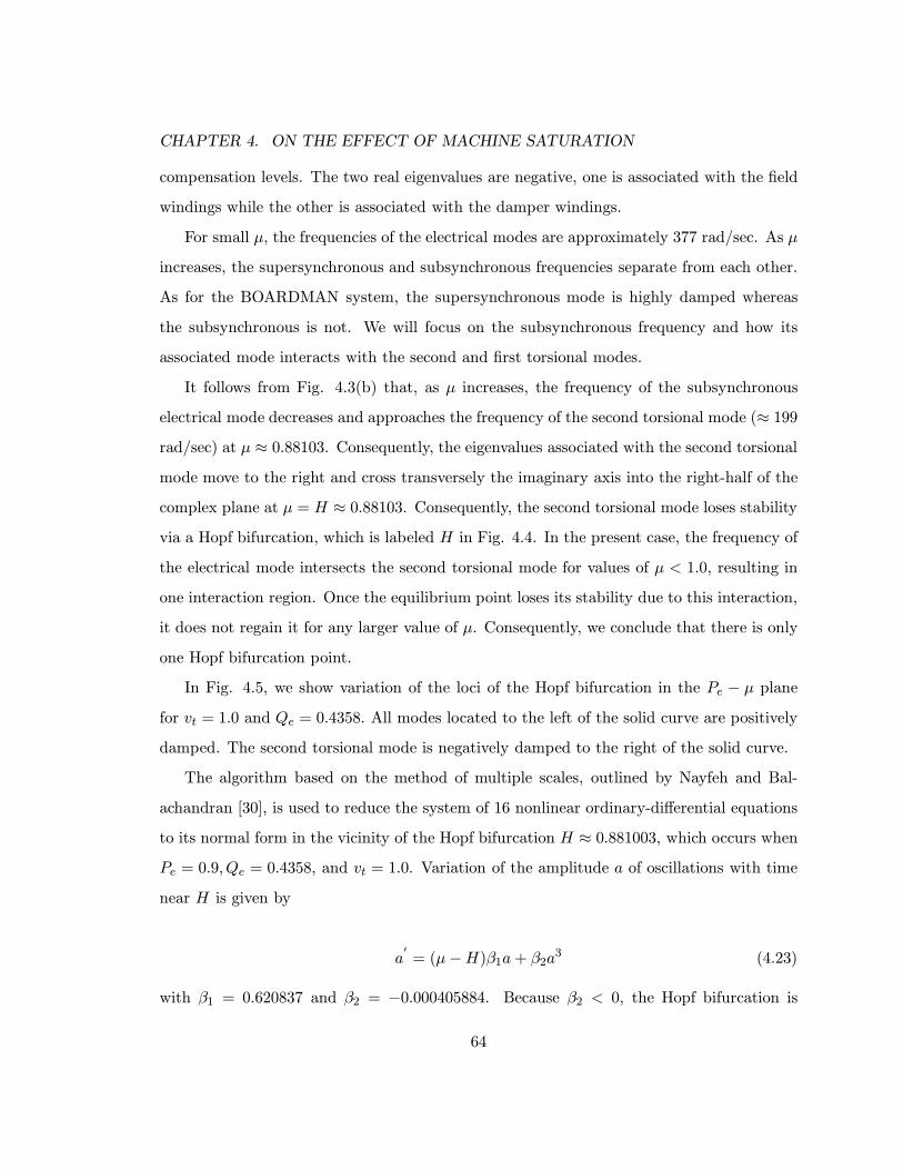
CHAPTER 4. ON THE EFFECT OF MACHINE SATURATION
compensation levels. The two real eigenvalues are negative, one is associated with the field
windings while the other is associated with the damper windings.
For small µ, the frequencies of the electrical modes are approximately 377 rad/sec. As µ
increases, the supersynchronous and subsynchronous frequencies separate from each other.
As for the BOARDMAN system, the supersynchronous mode is highly damped whereas
the subsynchronous is not. We will focus on the subsynchronous frequency and how its
associated mode interacts with the second and first torsional modes.
It follows from Fig. 4.3(b) that, as µ increases, the frequency of the subsynchronous
electrical mode decreases and approaches the frequency of the second torsional mode (≈ 199
rad/sec) at µ ≈ 0.88103. Consequently, the eigenvalues associated with the second torsional
mode move to the right and cross transversely the imaginary axis into the right-half of the
complex plane at µ = H ≈ 0.88103. Consequently, the second torsional mode loses stability
via a Hopf bifurcation, which is labeled H in Fig. 4.4. In the present case, the frequency of
the electrical mode intersects the second torsional mode for values of µ < 1.0, resulting in
one interaction region. Once the equilibrium point loses its stability due to this interaction,
it does not regain it for any larger value of µ. Consequently, we conclude that there is only
one Hopf bifurcation point.
In Fig. 4.5, we show variation of the loci of the Hopf bifurcation in the Pe − µ plane
for vt = 1.0 and Qe = 0.4358. All modes located to the left of the solid curve are positively
damped. The second torsional mode is negatively damped to the right of the solid curve.
The algorithm based on the method of multiple scales, outlined by Nayfeh and Bal-
achandran [30], is used to reduce the system of 16 nonlinear ordinary-differential equations
to its normal form in the vicinity of the Hopf bifurcation H ≈ 0.881003, which occurs when
Pe = 0.9, Qe = 0.4358, and vt = 1.0. Variation of the amplitude a of oscillations with time
near H is given by
a′= (µ−H)β1a+ β2a
3 (4.23)
with β1 = 0.620837 and β2 = −0.000405884. Because β2 < 0, the Hopf bifurcation is
64
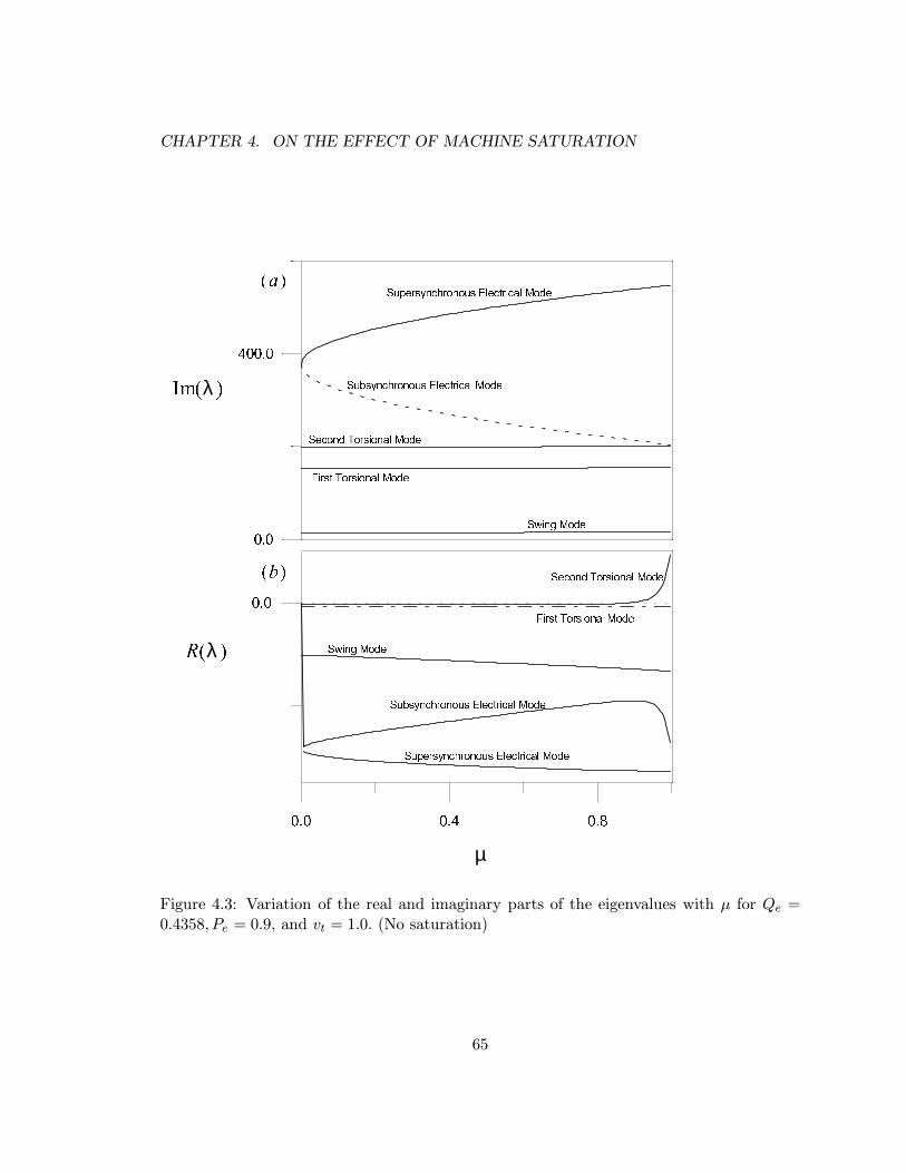
CHAPTER 4. ON THE EFFECT OF MACHINE SATURATION
0.0 0.4 0.8
0.0
0.0
400.0
Supersynchronous Electrical Mode
Subsynchronous Electrical Mode
Second Torsional Mode
First Torsional Mode
Swing Mode
Second Torsional Mode
First Torsional Mode
Swing Mode
Subsynchronous Electrical Mode
Supersynchronous Electrical Mode
R( )λ
Im( )λ
µ
( )a
( )b
Figure 4.3: Variation of the real and imaginary parts of the eigenvalues with µ for Qe =0.4358, Pe = 0.9, and vt = 1.0. (No saturation)
65

CHAPTER 4. ON THE EFFECT OF MACHINE SATURATION
0.8 0.9 1.0
0.72
0.74
0.76
δr
µ
SHH
Figure 4.4: Variation of the rotor angle δr with the compensation level µ for the casePe = 0.9, Qe = 0.4358, and vt = 1.0. The solid line denotes stable equilibria and the dashedline denotes unstable equilibria. The symbols H and SH indicate the compensation levelswhere the Hopf and seconary Hopf bifurcations occur, respectively. (No saturation)
66
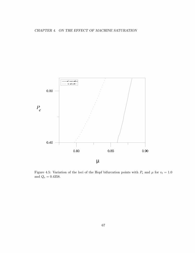
CHAPTER 4. ON THE EFFECT OF MACHINE SATURATION
0.80 0.85 0.90
0.40
0.80
µ
Pe
-------- with saturation
no saturation
Figure 4.5: Variation of the loci of the Hopf bifurcation points with Pe and µ for vt = 1.0and Qe = 0.4358.
67

CHAPTER 4. ON THE EFFECT OF MACHINE SATURATION
supercritical and the limit cycles born as a result of the bifurcation are stable. Their
amplitudes are given by
a = 39.11√µ−H (4.24)
The growth and stability of the limit cycles when µmoves away from the Hopf bifurcation
inside the unstable region has been studied by a combination of a two-point boundary-value
scheme and Floquet theory [30]. As µ increases from H, the limit cycle grows in size while
remaining stable with one Floquet multiplier being unity and the 15 remaining Floquet
multipliers lying inside the unit circle. See Fig. 4.6(a) for an example of a limit cycle.
When µ passes a critical value SH ≈ 0.88215, two of the Floquet multipliers exit the unit
circle away from the real axis, signifying that SH is a secondary Hopf bifurcation. There, the
limit cycle loses stability and gives way to a two-period quasiperiodic (two-torus) attractor,
which is displayed in Figs. 4.6(b) and (c). The corresponding time histories suggest that
the oscillations have two incommensurate periods. The FFT of δr seems to consist of two
incommensurate frequencies, their multiples, and combinations.
As µ increases slightly above SH to C ≈ 0.89976, the two-torus collides with its basin
boundary, yielding their destruction in a bluesky catastrophe. This can be observed in Fig.
4.7, which displays the time histories of δr and ωr in the vicinity of the bluesky catstrophe.
4.3 The Case of Saturation
In this section, we study the effect of the iron saturation. The parameters used
are those of the CHOLLA#4 model of the Arizona Public Service Company shown in Fig.
4.2.
Figure 4.8 shows variation of the real and imaginary parts of the eigenvalues with µ. It
follows from Fig. 4.8(b) that, as µ increases, the frequency of the subsynchronous electrical
mode decreases and approaches the frequency of the second torsional mode (≈ 199 rad/sec)
at µ ≈ 0.842003. Consequently, the eigenvalues associated with the second torsional mode
68

CHAPTER 4. ON THE EFFECT OF MACHINE SATURATION
δ r
δ r
δ r
ωr
( )a
( )b
( )c
Figure 4.6: Two-dimensional projections of the phase portrait onto the ωr − δr plane(left),the FFT of the corresponding generator rotor angle δr (middle), and the time traces ofthe generator rotor angle δr (right) at µ = (a) 0.880981, (b) 0.88598, and (c) 0.889760.The solution at (a) is a limit cycle, at (b) is a two-torus attractor recorded well before thebluesky catastrophe, and at (c) is a two-torus attractor located just before it disappears ina bluesky catastrophe.
69
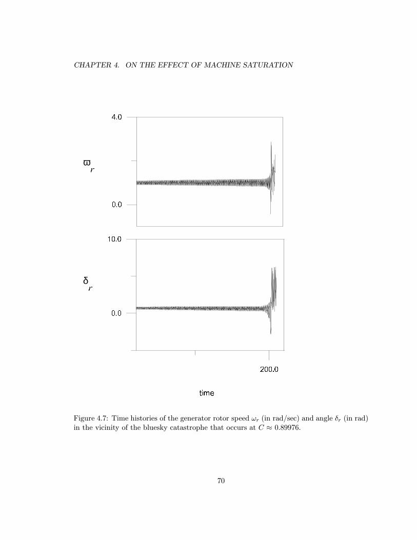
CHAPTER 4. ON THE EFFECT OF MACHINE SATURATION
200.0
0.0
10.0
0.0
4.0
ωr
δr
time
Figure 4.7: Time histories of the generator rotor speed ωr (in rad/sec) and angle δr (in rad)in the vicinity of the bluesky catastrophe that occurs at C ≈ 0.89976.
70
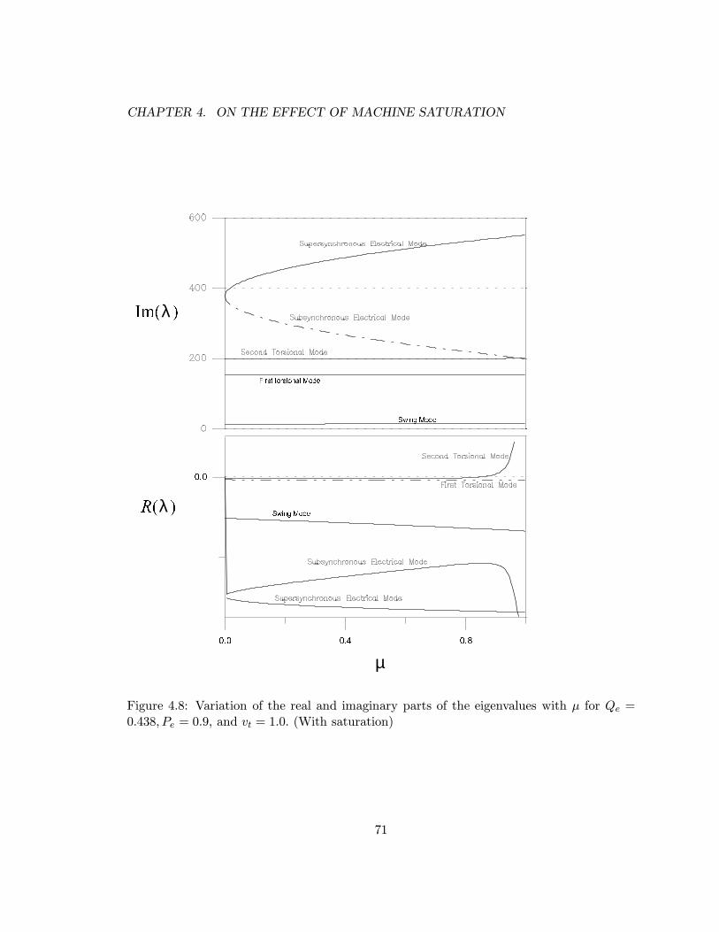
CHAPTER 4. ON THE EFFECT OF MACHINE SATURATION
0.0 0.4 0.8
0.0
Swing Mode
First torsional Mode
Swing Mode
R( )λ
Im( )λ
µ
Figure 4.8: Variation of the real and imaginary parts of the eigenvalues with µ for Qe =0.438, Pe = 0.9, and vt = 1.0. (With saturation)
71

CHAPTER 4. ON THE EFFECT OF MACHINE SATURATION
0.80 0.90 1.00
0.60
0.62
δr
µ
HSH
Figure 4.9: Variation of the rotor angle δr with the compensation level µ for the casePe = 0.9, Qe = 0.4358, and vt = 1.0. The solid line denotes stable equilibria and the dashedline denotes unstable equilibria. The symbols H and SH indicate the compensation levelsat which the Hopf and secondary Hopf bifurcations occur. (With saturation)
72

CHAPTER 4. ON THE EFFECT OF MACHINE SATURATION
move to the right and cross transversely the imaginary axis into the right-half of the complex
plane at µ = H ≈ 0.842003. There, the second torsional mode loses stability via a Hopf
bifurcation, which is labeled H in Fig. 4.8.
Figure 4.9 shows variation of the rotor angle δr with the compensation level µ. We
observe that the Hopf bifurcation point occurred at µ = H ≈ 0.842003. Comparing Fig. 4.4
with Fig. 4.9, we see that, in the case of saturation, the Hopf bifurcation occurs at a smaller
value of µ, namely, 0.842003 compared with µ ≈ 0.881003 for the case of no saturation. In
other words, the Hopf bifurcation point is shifted to the left. The iron saturation results in
a shrinking of the positively damped region, implying a destabilization of the system. To
show the destabilization of the iron saturation, we show in Fig. 4.5 variation of the loci of
the Hopf bifurcation in the Pe − µ plane for vt = 1.0 and Qe = 0.4358. All modes located
to the left of the dashed curve are positively damped whereas the second torsional mode
is negatively damped to the right of the dashed curve. It follows from Fig. 4.5 that the
iron saturation decreases the compensation level value at which subsynchronous resonance
occurs for all values of Pe. The smaller the value of Pe is, the more the destabilization of
the iron saturation is.
Again, the method of multiple scales is used to reduce the system of nonlinear ordinary-
differential equations to its normal form given by Eq. (4.23) in the vicinity of the Hopf
bifurcation H. For Pe = 0.9, Qe = 0.4358, and vt = 1.0, we find that β1 = 0.59695 and
β2 = −0.000213555. Because β2 < 0, the Hopf bifurcation H ≈ 0.842003 is supercritical
and the limit cycles born as a result of the bifurcation are stable. Their amplitudes are
given by
a = 52.8705√µ−H (4.25)
Again, the growth and stability of the limit cycles has been studied by means of a
combination of a two-point boundary-value scheme and Floquet theory [30]. As µ increases
from H, the limit cycle grows in size while remaining stable with one Floquet multiplier
being unity and the 15 remaining Floquet multipliers lying inside the unit circle. See Fig.
73

CHAPTER 4. ON THE EFFECT OF MACHINE SATURATION
4.10(a) for an example of a limit cycle.
When µ increases beyond a critical value SH ≈ 0.846651, two of the Floquet multipliers
exit the unit circle away from the real axis, signifying that SH is a secondary Hopf bifur-
cation. There, the limit cycle loses stability and gives way to a two-period quasiperiodic
(two-torus) attractor, which is displayed in Figs. 4.10(b) and (c). The corresponding time
histories suggest that the oscillations have two incommensurate periods. The FFT of δr
seems to consist of two incommensurate frequencies, their multiples, and combinations.
As µ increases slightly above SH to C ≈ 0.897651, the two-torus collides with its basin
boundary, yielding their destruction in a bluesky catastrophe. This can be observed in Fig.
4.11, which displays the time histories of δr and ωr in the vicinity of the bluesky catstrophe.
74

CHAPTER 4. ON THE EFFECT OF MACHINE SATURATION
δ r
δr
δ r
ω r
( )a
( )b
( )c
Figure 4.10: Two-dimensional projections of the phase portrait onto the ωr− δr plane(left),the FFT of the corresponding generator rotor angle δr (middle), and the time traces ofthe generator rotor angle δr (right) at µ = (a) 0.842351, (b) 0.848651, and (c) 0.887651.The solution at (a) is a limit cycle, at (b) is a two-torus attractor recorded well before thebluesky catastrophe, and at (c) is a two-torus attractor located just before it disappears ina bluesky catastrophe.
75
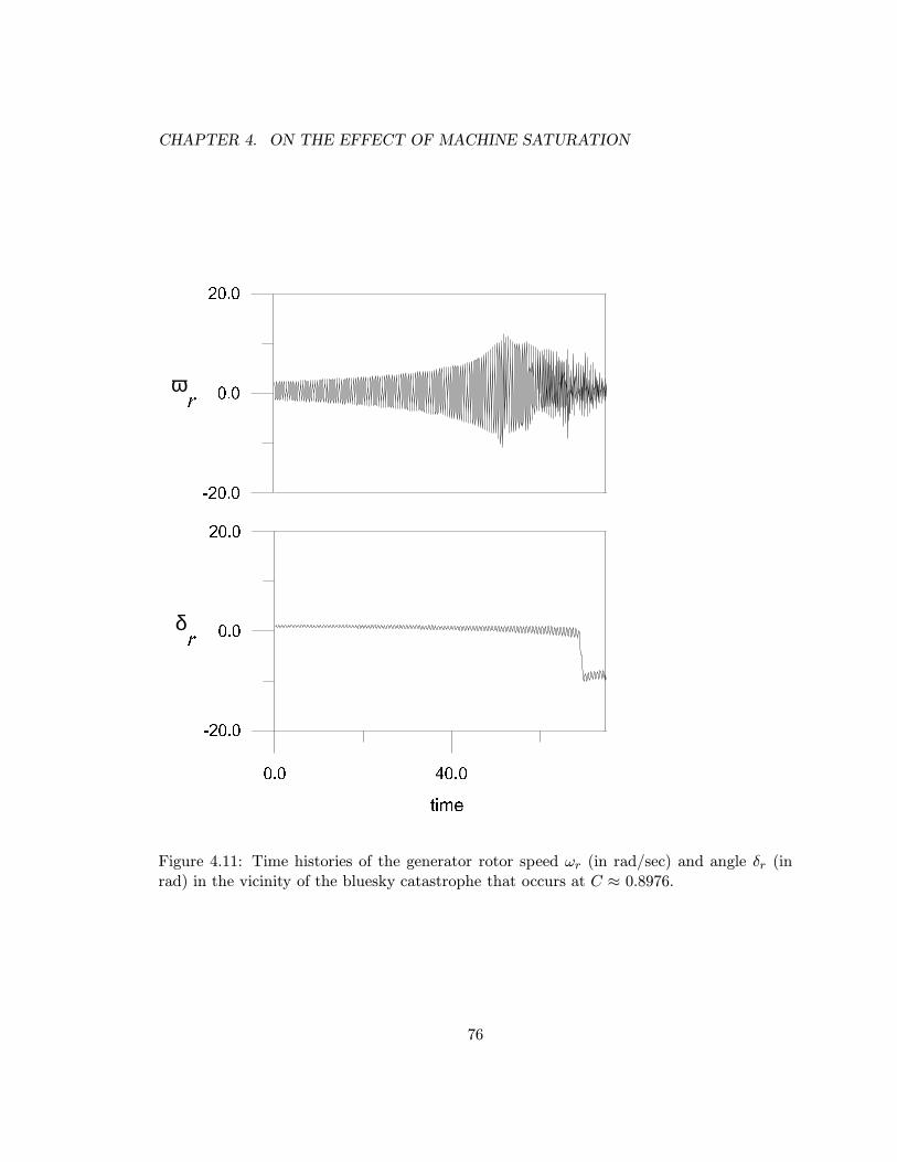
CHAPTER 4. ON THE EFFECT OF MACHINE SATURATION
-20.0
0.0
20.0
0.0 40.0
-20.0
0.0
20.0
δr
ωr
time
Figure 4.11: Time histories of the generator rotor speed ωr (in rad/sec) and angle δr (inrad) in the vicinity of the bluesky catastrophe that occurs at C ≈ 0.8976.
76

Chapter 5
CONTROL OF SSR
In this chapter, we investigate linear and nonlinear schemes to control subsynchronous
resonance. Two cases have been studied. First, we analyze the CHOLLA#4model including
the dynamics of a static excitation of the ST3 type. Then, we include the dynamics of a
power system stabilizer PSS. The study shows that the excitation system destabilizes the
CHOLLA#4 system by shrinking the stable region, whereas the PSS stabilizes the system
by expanding the stable region. A nonlinear controller that reduces the amplitudes of the
limit cycles has been designed.
5.1 Excitation System
The main function of an excitation system is to provide field current to the synchronous
machine. Early excitation systems were controlled manually to maintain the desired gen-
erator terminal voltage and reactive power loading [58-67]. When the voltage control was
first automated, it was very slow. At the beginning of 1920, the potential for enhancing
small signal and transient stability through use of continuous and fast acting regulators was
recognized. In the early 1960s, the role of the excitation system was expanded by using
auxiliary stabilizing signals, in addition to the terminal voltage error signal, to control the
field voltage and, hence, damp off oscillations. This part of the excitation control is known
as the power system stabilizer (PSS) [62 and 64].
The general functional block diagram in Fig. 5.1 indicates the various generator exci-
tation subsystems, which are used in the studies of electric power systems. It consists of
a terminal voltage transducer and load compensator, a voltage regulator, an exciter, an
77
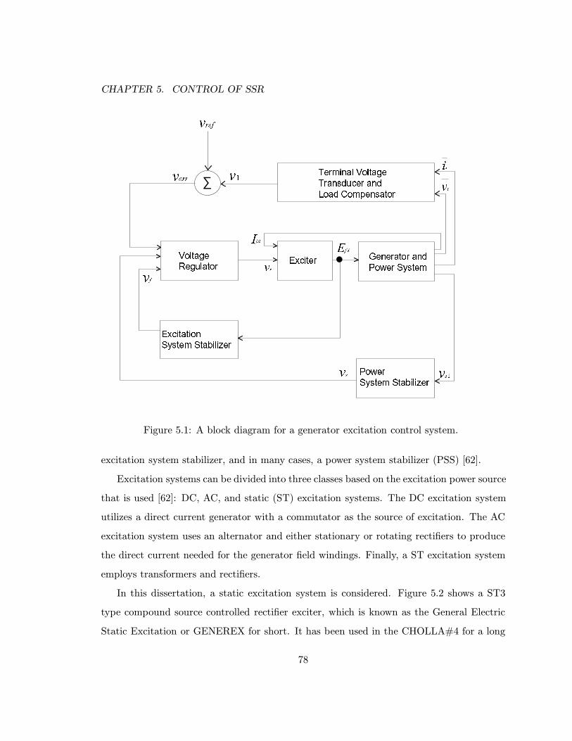
CHAPTER 5. CONTROL OF SSR
Terminal Voltage
Transducer and
Load Compensator
Generator and
Power SystemExciter
VoltageRegulator
Excitation
System Stabilizer
Power
System Stabilizer
∑
vref
verr v1
vf
vs vs1
vr
it
vt
Ifd
Efd
Figure 5.1: A block diagram for a generator excitation control system.
excitation system stabilizer, and in many cases, a power system stabilizer (PSS) [62].
Excitation systems can be divided into three classes based on the excitation power source
that is used [62]: DC, AC, and static (ST) excitation systems. The DC excitation system
utilizes a direct current generator with a commutator as the source of excitation. The AC
excitation system uses an alternator and either stationary or rotating rectifiers to produce
the direct current needed for the generator field windings. Finally, a ST excitation system
employs transformers and rectifiers.
In this dissertation, a static excitation system is considered. Figure 5.2 shows a ST3
type compound source controlled rectifier exciter, which is known as the General Electric
Static Excitation or GENEREX for short. It has been used in the CHOLLA#4 for a long
78
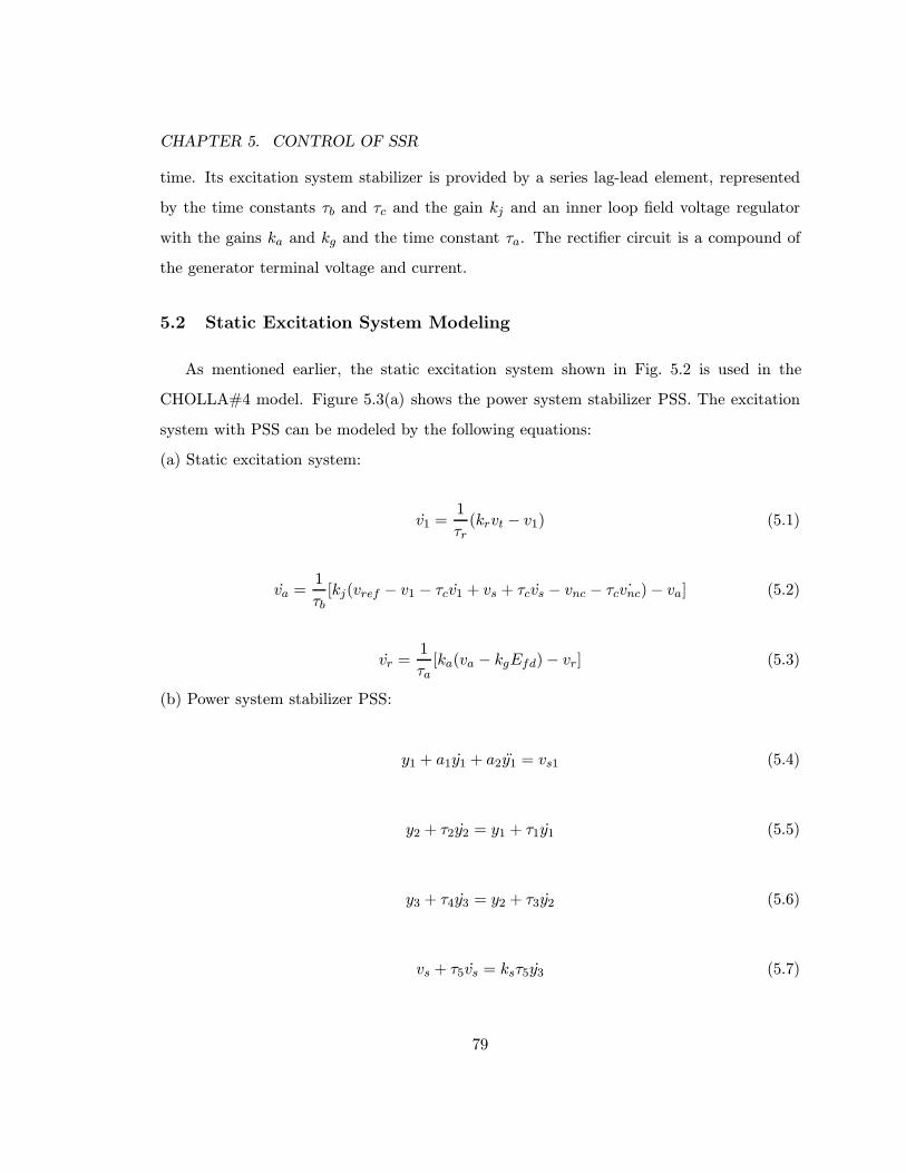
CHAPTER 5. CONTROL OF SSR
time. Its excitation system stabilizer is provided by a series lag-lead element, represented
by the time constants τb and τc and the gain kj and an inner loop field voltage regulator
with the gains ka and kg and the time constant τa. The rectifier circuit is a compound of
the generator terminal voltage and current.
5.2 Static Excitation System Modeling
As mentioned earlier, the static excitation system shown in Fig. 5.2 is used in the
CHOLLA#4 model. Figure 5.3(a) shows the power system stabilizer PSS. The excitation
system with PSS can be modeled by the following equations:
(a) Static excitation system:
v1 =1
τr(krvt − v1) (5.1)
va =1
τb[kj(vref − v1 − τcv1 + vs + τcvs − vnc − τc ˙vnc)− va] (5.2)
vr =1
τa[ka(va − kgEfd)− vr] (5.3)
(b) Power system stabilizer PSS:
y1 + a1y1 + a2y1 = vs1 (5.4)
y2 + τ2y2 = y1 + τ1y1 (5.5)
y3 + τ4y3 = y2 + τ3y2 (5.6)
vs + τ5vs = ksτ5y3 (5.7)
79

CHAPTER 5. CONTROL OF SSR
GenΠ
Π
Σ
ΣΣEfd
Vth
Ifd
+
+++ −
−
−
vref
v 1
vr
vb
vg
va
k
s
r
r1+ τ
kg
k
s
a
a1+ τks
sj
c
b
1
1
++
ττ
verr
vs
vnc
FEX
F f IEX N= ( ) I kI
VN c
fd
th
=IN
K K ej
k jkp p
p
pr pi= = +θ
V K v j K K X ith p t i p ex t= + +( )
it
vt
f I IN N( ) .= −1 0 58
= −0 752. ( )IN
= −1 732 1. ( )IN
when
when
when
IN ≤ 0 433.
0 433 0 75. .< >IN
1 0 0 75. .≥ ≥IN
Figure 5.2: A static excitation system of the ST3 type, which is a compound source con-trolled rectifier exciter (GENEREX).
80

CHAPTER 5. CONTROL OF SSR
High-Frequency Filter
1
1 1
2
2+ +sa s a
vs 1 = ∆ω
y3
y1
y21
1
1
2
++s
s
ττ
1
1
3
4
++s
s
ττ k
s
sc
ττ5
51+
vs max
vs min
vs
kvs 1
2
= ∆ω vnc
( )a
( )b
Figure 5.3: a) Power system stabilizer (PSS) and b) nonlinear controller.
81

CHAPTER 5. CONTROL OF SSR
Here, vt is the terminal generator voltage; v1 is the output of the terminal transducer; kr
and τr are the gain and time constant of the transducer, respectively; va is the regulator
internal voltage; vs is the power system stabilizer output; vnc is the quadratic controller
output signal; τa,τb, and τc are the voltage regulator time constants; vref is the reference
voltage; vr is the voltage regulator output; Efd is the exciter output voltage (generator field
voltage); ka is the voltage regulator gain; kg is the inner loop feedback constant; a1 and a2
are the PSS high frequency filter constants; vs1 is the power system stabilizer input; τ1 and
τ3 are the PSS lead compensating time constants; τ2 and τ4 are the PSS lag compensating
time constants; τ5 is the PSS washout time constant; and ks is the power system stabilizer
gain.
Equations (5.1)-(5.3) represent the dynamics of the static exciter and Eqs. (5.4)-(5.7)
represent the dynamics of the power system stabilizer. The total number of equations that
describe the system is 23. The first 16 equations represent the system, which was described
in Chapter 4, while the remaining 7 equations represent the dynamics of the excitation
system with PSS. In addition to the parameters given in Chapter 4, we let
kj = 200, τb = 10, τc = 1.0, kc = 1.13, τa = 1.0,
ka = 7.97, kg = 1.0, kr = 1.0, τr = 0.001, vrmax = 1.0,
vrmin = 0.0 a1 = 0.061, a2 = 0.0017,
τ1 = 0.3, τ2 = 0.03, τ3 = 0.3, τ4 = 0.03, τ5 = 10.0,
ks = 5.0, vsmax = 0.05, vsmin = −0.05, and k = 0
Again all the voltages are given in p.u. and the time constants are given in seconds. When
the PSS and the nonlinear controller are neglected, we set vs = vnc = 0 in Eq. (5.2) and
obtain
va =1
τb[kj(vref − v1 − τcv1)− va] (5.8)
82

CHAPTER 5. CONTROL OF SSR
5.3 Operating Conditions and Their Stability
The operating conditions (equilibrium solutions or points) can be obtained by setting
the derivatives of the state variables in the system of equations (4.7)-(4.22), (5.1), (5.3),
and (5.8) equal to zero. The result is
(R` +Ra)id −X`iq + ecd + v0 sin δr + ψq = 0 (5.9)
X`id + (R` +Ra)iq + ecq + v0 cos δr − ψd = 0 (5.10)
vf −Rf if = 0 (5.11)
ecd = µX`iq (5.12)
ecq = −µX`id (5.13)
Tm = iqψd − idψq (5.14)
ωr = ω1 = ω2 = ω3 = ω4 = 1 (5.15)
δr = θ1 = θ2 = θ3 = θ4 (5.16)
kr(v2d + v2q )
12 − v1 = 0 (5.17)
kj(vref − v1)− va = 0 (5.18)
ka(va − kgvrvb)− vr = 0 (5.19)
Instead of specifying Tm and v0, one usually specifies the real Pe and reactive Qe powers.
In p.u., these control parameters are related to the voltages and currents through
Pe = vdid + vqiq (5.20)
Qe = vqid − vdiq (5.21)
To relate the voltages vd and vq to the currents id, iq, and if , we note that, at the operating
condition, Eqs. (3.1) and (3.2) reduce to
vd = −Raid − ψq (5.22)
83

CHAPTER 5. CONTROL OF SSR
vq = −Raiq + ψd (5.23)
Using Eqs. (4.3) and (4.4) to eliminate ψd and ψq from Eqs. (5.9), (5.10), (5.14), (5.22),
and (5.23) yields
(R` +Ra)id −X`iq + µX`iq + v0 sin δr + [q0 − q1iq + q2i2q − q3i
3q −Xleiq] = 0 (5.24)
X`id + (R` +Ra)iq − µX`id + v0 cos δr
−[d0 + d1(−id + if ) + d2(−id + if )2 + d3(−id + if )
3 −Xleid] = 0 (5.25)
Tm = iq[d0 + d1(−id + if ) + d2(−id + if )2 + d3(−id + if )
3 −Xleid]
−id[q0 − q1iq + q2i2q − q3i
3q −Xleiq] (5.26)
vd = −Raid − [q0 − q1iq + q2i2q − q3i
3q −Xleiq] (5.27)
vq = −Raiq + [d0 + d1(−id + if ) + d2(−id + if )2 + d3(−id + if )
3 −Xleid] (5.28)
where
vf = vbvrRf
d1= Rf if (5.29)
vb = [(w21 + w2
2)12 − 0.58kcd1if ] when IN ≤ 0.433
= [0.75(w21 + w2
2)− (d1ifkc)2]
12 when 0.75 < IN < 0.433
= 1.732[(w21 + w2
2)12 − kcd1if ] when 1.0 ≥ IN ≥ 0.75 (5.30)
IN =kcd1if
(w21 + w2
2)12
(5.31)
w1 = kprvd − kpivq −KI iq − kprXexiq − kpiXexid (5.32)
w2 = kpivd + kprvq +KI id + kprXexid − kpiXexiq (5.33)
Given Pe, Qe, and µ = Xc/X`, we solve the algebraic system of ten equations given
by Eqs. (5.11), (5.17)-(5.21), (5.24), (5.25), and (5.27)-(5.28) to determine the nine state
84

CHAPTER 5. CONTROL OF SSR
variables id, iq, if , vd, vq, v1, va, vr, and δr and the control parameter v0. Then, we calculate
Tm from Eq. (5.26), thereby determining the operating condition and the control parameters
v0 and Tm. Using an arclength continuation scheme [30], we calculate variation of the
operating condition (equilibrium point) with the control parameter µ.
The stability of a given equilibrium point is ascertained by examination of the eigenvalues
of the Jacobian matrix J of equations (4.7)-(4.22), (5.1)-(5.3), and (5.36)-(5.40) evaluated at
the equilibrium point. The equilibrium point is stable if all of the eigenvalues of the Jacobian
matrix lie in the left-half of the complex plane and unstable if at least one eigenvalue lies
in the right-half of the complex plane.
5.4 The Case without PSS
In this section, we study the effect of the excitation system without PSS on subsyn-
chronous resonance using the modern methods of nonlinear dynamics.
When Pe = 0.9 and Qe = 0.4358, we show in Fig. 5.4 variation of the real and imaginary
parts of the eigenvalues with µ. There are 14 complex and five real eigenvalues. Because
the Jacobian matrix is real, the complex conjugate of each complex value is an eigenvalue,
yielding 7 oscillatory modes. Two modes are electrical modes and 5 are mechanical modes.
The mode with the lowest frequency is the swing or electro-mechanical mode whereas the
other four mechanical modes are torsional modes. Two of the torsional modes, the third and
fourth modes, are damped and have very high frequencies, namely, 1030 and 1450 rad/sec.
Hence, they do not interact with the electrical modes for realistic compensation levels. The
five real eigenvalues are negative, two are associated with the field and damper windings,
while the other three are associated with the excitation system.
For small µ, the frequencies of the electrical modes are approximately 377 rad/sec. As µ
increases, the supersynchronous and subsynchronous frequencies separate from each other.
As for the BOARDMAN system, the supersynchronous mode is highly damped whereas
the subsynchronous is not. We will focus on the subsynchronous frequency and how its
85

CHAPTER 5. CONTROL OF SSR
0.0 0.5 1.0
0.0
second torsional mode
first torsional mode
swing mode
subsynchronous electrical mode
supersynchronous electrical mode
0.0
400.0
supersynchronous electrical mode
subsynchronous electrical mode
second torsional mode
first torsional mode
swing mode
Im( )λ
R( )λ
µ
( )a
( )b
Figure 5.4: Variation of the real and imaginary parts of the eigenvalues with µ for Qe =0.4358 and Pe = 0.9, (Without PSS)
86

CHAPTER 5. CONTROL OF SSR
associated mode interacts with the second and first torsional modes.
It follows from Fig. 5.4(a) that, as µ increases, the frequency of the subsynchronous
electrical mode decreases and approaches the frequency of the second torsional mode (≈ 199
rad/sec) at µ ≈ 0.819. Consequently, the eigenvalues associated with the second torsional
mode move to the right and cross transversely the imaginary axis into the right-half of the
complex plane at µ = H ≈ 0.819. Consequently, the second torsional mode loses stability
via a Hopf bifurcation, which is labeled H in Fig. 5.5. In the present case, the frequency
of the electrical mode intersects the second torsional mode for values of µ < 1.0, resulting
in one interaction region. Once the equilibrium point loses stability due to this interaction,
it does not regain it for any larger value of µ. Consequently, we conclude that there is only
one Hopf bifurcation point.
Figure 5.5 shows variation of the generator rotor angle δr with the compensation level
µ. One can see that the Hopf bifurcation point H is shifted to the left from µ = 0.842 to
µ = 0.819. In other words, the positively damped region or the stable region is decreased.
So, the excitation system is destabilizing the system.
We now resort to the method of multiple scales to reduce the new system of 19 first-order
nonlinear ordinary-differential equations to its normal form near the Hopf bifurcation point
H at µ = µo. For Pe = 0.9 and Qe = 0.4358, variation of the amplitude a of the oscillations
with time near H of Fig. 5.5 is given by
a′= (µ−H)β1a+ β2a
3 (5.34)
with β1 = 0.523413 and β2 = −0.000623183. Thus, the Hopf bifurcation H ≈ 0.819 is
supercritical and the limit cycles born as a result of the bifurcation are stable. Their
amplitudes are given by
a = 28.98√µ−H (5.35)
87

CHAPTER 5. CONTROL OF SSR
0.8 1.0
0.60
0.62
0.64
H = 0 819.
H = 0 842.
1
2
δr
µ
Figure 5.5: Bifurcation diagram showing variation of the generator rotor angle δr with thecompensation level µ. Line 2 corresponds to the case without the excitation system andthe PSS, and line 1 corresponds to the case with the excitation system only. The solid linesdenote sinks and the dashed lines denote unstable foci.
88

CHAPTER 5. CONTROL OF SSR
5.5 The Case with PSS
The main function of PSS is to improve the dynamic stability of power systems. Intensive
effort to improve power system stability has resulted in the widespread use of other regulator
input signals in addition to the terminal voltage. These signals are chosen to provide positive
damping to the oscillations [62]. In synchronous condenser applications, the objective most
frequently used is to minimize voltage swings. Figure 5.3(a) shows the generalized form of
such a power system stabilizer. Some common stabilizer input signals include accelerating
power, speed deviation, frequency deviation, and terminal voltage. They are designated by
vs1.
The first block represents a high-frequency filter. The next two blocks allow two stages
of lead-lag compensation. The stabilizer gain is set by ks and signal washout is set by the
time constant τ5. The stabilizer output can be limited in many ways. Figure 5.3(a) shows
simple output limits. In other systems, the stabilizer output is limited by the generator
terminal voltage. The stabilizer output vs is added to the terminal voltage error signal at
the location shown in Fig. 5.2.
The dynamics of the PSS, which is shown in Fig. 5.3(a) and given by Eqs. (5.4)-
(5.7), consists of a second-order ordinary-differential equation and three first-order ordinary-
differential equations. We let y1 = x1 and y1 = x2 and rewrite Eqs. (5.4)-(5.7) as
x1 = x2 (5.36)
x2 =1
a2(vs1 − x1 − a1x2) (5.37)
y2 =1
τ2(x1 + τ1x2 − y2) (5.38)
y3 =1
τ4(y2 + τ3y2 − y3) (5.39)
89
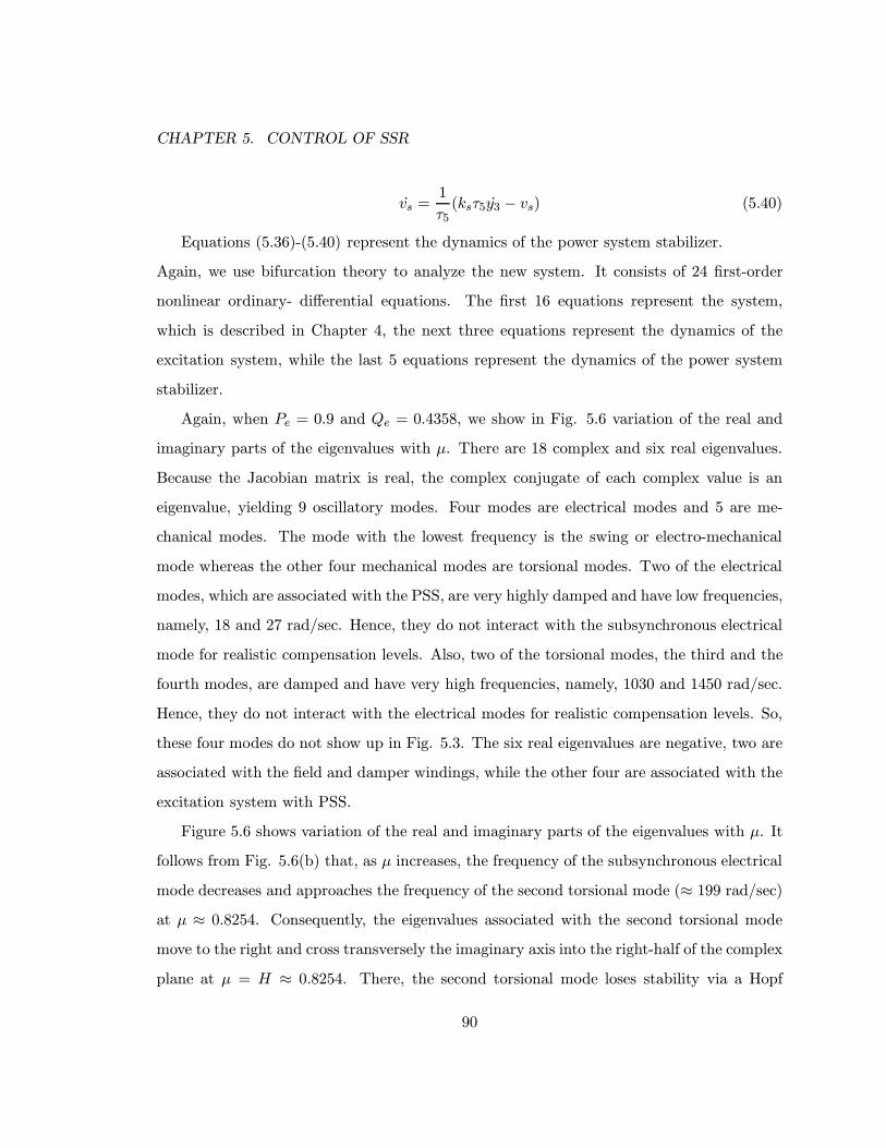
CHAPTER 5. CONTROL OF SSR
vs =1
τ5(ksτ5y3 − vs) (5.40)
Equations (5.36)-(5.40) represent the dynamics of the power system stabilizer.
Again, we use bifurcation theory to analyze the new system. It consists of 24 first-order
nonlinear ordinary- differential equations. The first 16 equations represent the system,
which is described in Chapter 4, the next three equations represent the dynamics of the
excitation system, while the last 5 equations represent the dynamics of the power system
stabilizer.
Again, when Pe = 0.9 and Qe = 0.4358, we show in Fig. 5.6 variation of the real and
imaginary parts of the eigenvalues with µ. There are 18 complex and six real eigenvalues.
Because the Jacobian matrix is real, the complex conjugate of each complex value is an
eigenvalue, yielding 9 oscillatory modes. Four modes are electrical modes and 5 are me-
chanical modes. The mode with the lowest frequency is the swing or electro-mechanical
mode whereas the other four mechanical modes are torsional modes. Two of the electrical
modes, which are associated with the PSS, are very highly damped and have low frequencies,
namely, 18 and 27 rad/sec. Hence, they do not interact with the subsynchronous electrical
mode for realistic compensation levels. Also, two of the torsional modes, the third and the
fourth modes, are damped and have very high frequencies, namely, 1030 and 1450 rad/sec.
Hence, they do not interact with the electrical modes for realistic compensation levels. So,
these four modes do not show up in Fig. 5.3. The six real eigenvalues are negative, two are
associated with the field and damper windings, while the other four are associated with the
excitation system with PSS.
Figure 5.6 shows variation of the real and imaginary parts of the eigenvalues with µ. It
follows from Fig. 5.6(b) that, as µ increases, the frequency of the subsynchronous electrical
mode decreases and approaches the frequency of the second torsional mode (≈ 199 rad/sec)
at µ ≈ 0.8254. Consequently, the eigenvalues associated with the second torsional mode
move to the right and cross transversely the imaginary axis into the right-half of the complex
plane at µ = H ≈ 0.8254. There, the second torsional mode loses stability via a Hopf
90

CHAPTER 5. CONTROL OF SSR
0.0 0.5 1.0
-4.0
0.0second torsional mode
subsynchronous torsional mode
supersynchronous electrical mode
first torsional mode
400.0
supersynchronous electrical mode
subsynchronous electrical mode
second torsional mode
first torsional mode
Im( )λ
R( )λ
µ
( )a
( )b
Figure 5.6: Variation of the real and imaginary parts of the eigenvalues with µ for Qe =0.4358 and Pe = 0.9, (With PSS)
91
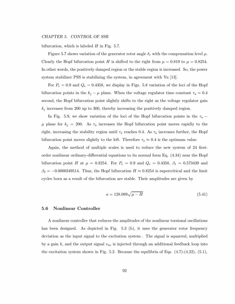
CHAPTER 5. CONTROL OF SSR
bifurcation, which is labeled H in Fig. 5.7.
Figure 5.7 shows variation of the generator rotor angle δr with the compensation level µ.
Clearly the Hopf bifurcation point H is shifted to the right from µ = 0.819 to µ = 0.8254.
In other words, the positively damped region or the stable region is increased. So, the power
system stabilizer PSS is stabilizing the system, in agreement with Yu [13].
For Pe = 0.9 and Qe = 0.4358, we display in Figs. 5.8 variation of the loci of the Hopf
bifurcation points in the kj − µ plane. When the voltage regulator time constant τa = 0.4
second, the Hopf bifurcation point slightly shifts to the right as the voltage regulator gain
kj increases from 200 up to 300, thereby increasing the positively damped region.
In Fig. 5.9, we show variation of the loci of the Hopf bifurcation points in the τa −µ plane for kj = 200. As τa increases the Hopf bifurcation point moves rapidly to the
right, increasing the stability region until τa reaches 0.4. As τa increases further, the Hopf
bifurcation point moves slightly to the left. Therefore τa ≈ 0.4 is the optimum value.
Again, the method of multiple scales is used to reduce the new system of 24 first-
order nonlinear ordinary-differential equations to its normal form Eq. (4.34) near the Hopf
bifurcation point H at µ = 0.8254. For Pe = 0.9 and Qe = 0.4358, β1 = 0.573439 and
β2 = −0.0000349514. Thus, the Hopf bifurcation H ≈ 0.8254 is supercritical and the limit
cycles born as a result of the bifurcation are stable. Their amplitudes are given by
a = 128.089√µ−H (5.41)
5.6 Nonlinear Controller
A nonlinear controller that reduces the amplitudes of the nonlinear torsional oscillations
has been designed. As depicted in Fig. 5.3 (b), it uses the generator rotor frequency
deviation as the input signal to the excitation system . The signal is squarred, multiplied
by a gain k, and the output signal vnc is injected through an additional feedback loop into
the excitation system shown in Fig. 5.2. Because the equilibria of Eqs. (4.7)-(4.22), (5.1),
92

CHAPTER 5. CONTROL OF SSR
0.7 0.8 0.9 1.0
0.60
0.62
0.64
δr
µ
H = 0 8254.
H = 0 842.
1
2
Figure 5.7: Bifurcation diagram showing variation of the generator rotor angle δr with thecompensation level µ. Line 2 corresponds to the case without the excitation system andthe PSS, and line 1 corresponds to the case with the excitation system and the PSS. Thesolid lines denote sinks and the dashed lines denote unstable foci.
93
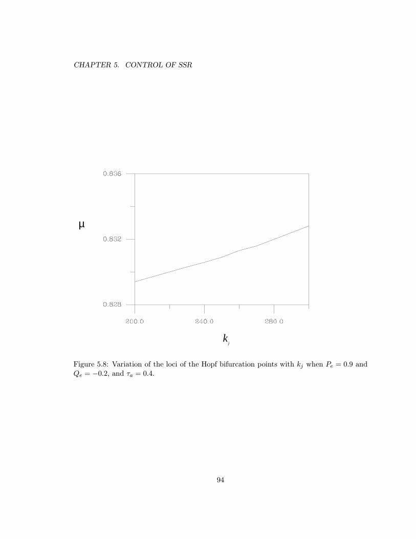
CHAPTER 5. CONTROL OF SSR
µ
kj
Figure 5.8: Variation of the loci of the Hopf bifurcation points with kj when Pe = 0.9 andQe = −0.2, and τa = 0.4.
94

CHAPTER 5. CONTROL OF SSR
µ
τa
Figure 5.9: Variation of the loci of the Hopf bifurcation points with τa when Pe = 0.9 andQe = −0.2, and kj = 200.
95
CHAPTER 5. CONTROL OF SSR
(5.3), (5.8), and (5.36)-(5.40) correspond to ∆ω = 0, this nonlinear controller does not
affect their locations. Moreover, because the cotribution of this nonlinear controller to the
Jacobian matrix of Eqs. (4.7)-(4.22), (5.1), (5.3), (5.8), and (5.36)-(5.40) evaluated at the
equilibria is zero, it does not affect their linear stability. However, this nonlinear controller
can have a significant effect on the dynamic behavior of the system. In other words, the
nonlinear controller does not affect the operating condition and the location of the Hopf
bifurcation, but it strongly affect the nonlinear behaviour of the power system.
Again, using the method of multiple scales, we reduce Eqs. (4.7)-(4.22), (5.1), (5.3),
(5.8), and (5.36)-(5.40) into the normal form given by Eq. (5.34) with β2 being replaced
with
β2 = β2 + kβ21 + k2β22 (5.42)
To study the effect of the gain on the performance of controller, we carry out a bifurcation
analysis as follows. For k = 100, we find that β2 = −0.00257164. Thus, the Hopf bifurcationH ≈ 0.8254 remains supercritical and the limit cycles born as a result of the bifurcations
remain stable. Their amplitudes are given by
a = 14.9327√µ−H (5.43)
For k = 500, we find that β2 = −0.0127184. Thus, the Hopf bifurcation H ≈ 0.8254
remains supercritical and the limit cycles born as a result of the bifurcations remain stable.
However, their amplitudes reduced to
a = 6.7147√µ−H (5.44)
Using the value of β2 at k = 0, 100 and 500, we find that, the coefficients in Eq. (5.42)
are β21 = −2.5366 × 10⁻⁵ and β22 = −7.55 × 10⁻¹⁴. With these values, we show in Fig.
5.10, variation of a, the amplitude of the limit-cycle born at H, with k. Because β2 is
negative, the Hopf bifurcation H = 0.8254 remains supercritical. Because | β2 | increases
96

CHAPTER 5. CONTROL OF SSR
0.0 400.0 800.0
0.0
50.0
100.0
k
a
Figure 5.10: Variation of a, the amplitude of the limit-cycle born at H, with the nonlinearcontroller gain k.
as k increases, the larger the value of k is, the smaller the amplitude of the limit-cycle born
at H is. Further increases in the gain k, one can suppress the secondary Hopf bifurcation
and hence the bluesky catastrophe.
97
Chapter 6
CONCLUSIONS
We have applied bifurcation theory together with the method of normal forms
and Floquet theory to a two practical series capacitor-compensated-single-machine power
systems: the BOARDMAN and CHOLLA#4 turbine-generator systems. For the BOARD-
MAN system, we have revealed the existence of complex self-excited oscillations of the
turbine-generator rotor, such as limit cycles and two-torus attractors, for practical com-
pensation values. We have shown that they result from a strong interaction of the sub-
synchronous electrical mode with either the second or third mechanical mode of a 5-mass
rotor. These oscillations can cause loss of fatigue life of the turbine-generator shaft and,
ultimately, can lead to its break with disastrous consequences. For high compensation val-
ues, they may induce loss of synchronism of the generator following the disappearance of
the two-torus attractor and its basin of attraction in a bluesky catastrophe. Next, we inves-
tigate the influence of adding damper windings along the q- and d-axes on subsynchronous
resonance. The study shows that these damper windings affect the locations and the type
of the Hopf bifurcations. Adding q-axis damper windings shifts the Hopf bifurcation to
smaller values of µ and changes it from supercritical to subcritical. In other words, q-axis
damper windings shrinks the stable region and may lead to loss of synchronism at a value
of µ below that which the Hopf bifurcation occurs.
Adding damper windings on either the d-axis or both q- and d-axes also shifts the Hopf
bifurcation to smaller value of µ and hence shrinks the stable region. However, the Hopf
bifurcation remains supercritical. In general, the damper windings distabilize the system
by reducing the compensation level at which subsynchronous resonance occurs.
For the CHOLLA#4 system, we use a complete turbine-generator model that includes
98

CHAPTER 6. CONCLUSIONS
the generator damper windings, the generator saturation, and the automatic voltage regu-
lator. Results similar to those of the BOARDMAN system have been obtained except that
there is only a single supercritical Hopf bifurcation instead of three.
We have studied the effect of the generator saturation on subsynchronous resonances
while neglecting the AVR system. The results show that the generator saturation shrinks the
positively damped region by shifting the Hopf bifurcation to smaller compensation levels.
To enlarge the stability region and damp off the torsional oscillations, we have investigated
linear and nonlinear controllers injected into the AVR system. The linear controller increases
the compensation level at which subsynchronous resonance occurs. On the other hand, the
nonlinear controller does not affect the location and type of the Hopf bifurcation H. The
study shows that, the larger the value of the nonlinear controller gain k is, the smaller the
amplitude of the limit-cycle born near H is. By increasing the gain k, one can suppress the
secondary Hopf bifurcation and hence the bluesky catastrophe.
Future research should continue to see the effect of machine saturation as well as the
dynamics of damper windings on subsynchronous resonance for different systems.
99
REFERENCES
[1] J. W. Ballance and S. Goldberg,“Subsynchronous Resonance in Series CompensatedTransmission Lines”, IEEE Trans. on PAS, pp 1649-1658, Sep./Oct. 1973.
[2] D. N. Walker, C. E. Bowler, R. L. Jackson, and D. A. Hodges,“Results of Subsyn-chronous Resonance Test at Mohave”, IEEE Trans. on PAS, pp 1878-1889, Sep./Oct.1975.
[3] R. G. Farmer, E. Katz, and A. L. Schwalb,“Navajo Project on Subsynchronous Reso-nance Analysis and Solutions”, IEEE Trans. on PAS, pp 1226-1232, July/Aug., 1977.
[4] IEEE Committee Report, “First Benchmark Model for Computer Simulation of Sub-synchronous Resonance,” IEEE Trans. on PAS, pp. 1565-1570, 1977.
[5] IEEE Committee Report, “Second Benchmark Model for Computer Simulation of Sub-synchronous Resonance,” IEEE Trans. on PAS, pp. 1057-1066, 1985.
[6] IEEE Power System Engineering Committee Report, “Terms, Definitions & Symbolsfor Subsynchronous Oscillations,” IEEE Trans. on PAS, pp. 1326-1334, 1985.
[7] IEEE Committee Report, “Reader’s Guide to Subsynchronous Resonance,” IEEETrans. on PAS, pp. 150-157, 1992.
[8] P. M. Anderson, B. L. Agrawal, and J. E. Van Ness, Subsynchronous Resonance inPower Systems, IEEE Press, New York, 1990.
[9] G. Gross and M. C. Hall, “Synchronous Machine and Torsional Dynamics Simulation inthe Computation of Electromagnetic Transients,” IEEE Trans. on PAS, pp. 1074-1085,1978.
[10] P. H. Beagles, K. Carlsen, M. L. Crenshaw, and M. Temoshok, “Generator and PowerSystem Performance with the GENERREX Excitation System”, IEEE Trans. on PAS,pp. 489-493, March/April 1976.
[11] A. Edris,“Series Compensation Schemes Reducing the Potential of Resonance”, IEEETrans. on PAS,pp. 219-226, Feb. 1990.
[12] L.A. Kilgore, D. G. Ramey, and M. C. Hall,“Simplified Transmission and GenerationAnalysis Procedures for SSR”, IEEE Trans. on PAS, pp 1840-1846 Nov./Dec. 1977.
100
REFERENCES
[13] R. D. Rana, S. W. Huff, R. M. Hayes, E. N. Fromholtz, and R. P. Schulz,“AEP’sKanawha River 345 KV Series Capacitor Installation- Subsynchronous Resonance Stud-ies and Torsional Measurements”, Proceedings of the American Power Conference,pp.300-305, 1991.
[14] Y. Yu, Electric Power System Dynamics, Academic Press, New York, 1983.
[15] A. A. Fouad and K. T. Khu,“Subsynchronous Resonance Zones in the IEEE BenchMark Power System”, IEEE Trans. on PAS, May/June 1978.
[16] A. Yan and Y. Yu,“Multi-Mode Stabiliztion of Torsional Oscillations Using OutputFeedback Excitation Control”, IEEE Trans. on PAS, May 1982.
[17] M. R. Iravani and A. A. Edris,“Eigen Analysis of Series Compensation Schemes Re-ducing the Potential of Subsynchronous Resonance”, IEEE Power System SummerMeeting, 1994.
[18] W. Zhu,“Analysis of Subsynchronous Resonance in Power Systems”, Ph.D Thesis,Oregon State University, June, 1994.
[19] M. R. Iravani and A. Semlyen,“Hopf Bifurcations in Torsional Dynamics (Turbine-Generator)”, IEEE Trans. on PAS, pp. 28-36, Feb. 1992.
[20] W. Zhu, R. R. Mohler, R. Spee, W. A. Mittelstadt, and D. Maratukulam,“ HopfBifurcations in a SMIB Power System with SSR”, IEEE Proceeding of the 1995 SummerMeeting, pp. 531-534, PWRS.
[21] W. Zhu, R. Spee, R. R. Mohler, G. G. Alexander, W. A. Mittelstadt, and D. Maratuku-lam,“An EMTP Study of SSR Mitigation Using the Thyristor Controlled Series Ca-pacitor”, IEEE Trans. on Power Delivery, 1995.
[22] E. H. Abed and P. Varaiya, “Nonlinear Oscillations in Power Systems,” InternationalJournal of Electric Power and Energy Systems, pp. 373-343, 1984.
[23] I. Dobson and H.-D. Chiang, “Towards a Theory of Voltage Collapse in Electric PowerSystems,” Syst. Control Ltrs.,, pp. 253-262, 1989.
[24] M. A. Nayfeh, A. M. A. Hamdan, and A. H. Nayfeh, “Chaos and Instability in a PowerSystem - Primary Resonant Case,” Nonl. Dyn., pp. 313-339, 1990.
[25] V. Venkatasubramanian, H. Schattler, and J. Zaborszky, “Voltage Dynamics: Studyof a Generator with Voltage Control, Transmission and Matched MW Load,” IEEETrans. Auto. Control, pp. 1717-1733, 1992.
[26] V. Ajjarapu and B. Lee, “Bifurcation Theory and its Application to Nonlinear Dynam-ical Phenomena in an Electrical Power System,” IEEE Trans., on PAS, pp. 424-431,1992.
101

REFERENCES
[27] E. H. Abed, H. Wang, J. C. Alexander, A. M. A. Hamdan, and H.-C. Lee, “DynamicBifurcations in a Power System Model Exhibiting Voltage Collapse,” Int. J. Bif. Chaos,pp. 1169-1176, 1993.
[28] W. Ji and V. Venkatasubramanian, ”Dynamics of a Minimal Power System: invarianttori and quasi-periodic motions,” IEEE Trans. Circuits Syst., pp. 981-1000, 1995.
[29] A. H. Nayfeh, A. M. Harb, and C.-M. Chin, ”Bifurcation in a Power System Model,”Int. J. Bif. Chaos, vol. 6, pp. 497-512, 1996.
[30] A. H. Nayfeh and B. Balachandran, Applied Nonlinear Dynamics, Wiley, New York,1995.
[31] A. Nayfeh, Introduction to Perturbation Techniques, Wiley, New-York, 1983
[32] A. Nayfeh, Perturbation Methods, Wiley, New-York, 1973
[33] P. Kundur, Power System Stability and Control, Electric Power Research Institute,McGraw-Hill, New York, 1994.
[34] R. G. Harly, D. J. Limebeer, and E. Chirricozzi,“Comparative Study of SaturationMethods in Synchronous Machine Models”, IEE Proc., vol. 127, Pt. B, January 1980.
[35] F. P. De Mello and L. N. Hannet,“Representation of Saturation in Synchronous Ma-chines”, IEEE Trans. on PAS, Nov. 1986
[36] A-R. A. M. Makky,“Representation of Saturated Salient-Pole Synchronous Machine byA Single Magnetization Curve”, Electric Machines and Electromechanics, vol. 7, pp.369-380, April 1982.
[37] A. M. El-Serafi and J. Wu,“Saturation Representation in Synchronous Machine Mod-els”, Electric Machines and Power Systems, vol. 20, pp. 355-369, August 1992.
[38] J. Lemay and T. H. Barton,“Small Perturbation Linearization of the Saturated Syn-chronous Machine Equations”, IEEE Trans. on PAS, pp. 233-240, Sept. 1971.
[39] A. H. Nayfeh and O. R. Asfar,“An Analytical Solution of the Nonlinear Eddy-CurrentLosses in Ferromagnetic Materials”, IEEE Trans. on Magnetics, vol. MAG-10, June1974.
[40] J. W. Dougherty and S. H. Minnich,“Finite Element Modeling of Large generators;Calculations Versus Load Test Data”, IEEE Trans. on PAS, August 1981.
[41] A. M. El-Serafi, A. s. Abdallah, M. K. Elsherbiny, and E. H. Badawy, “ExperimentalStudy of the Saturation and the Cross-Magnetizing Phenomenon in Saturated Syn-chronous Machines”, IEEE Trans. Energy Conversion, vol. 3
102

REFERENCES
[42] M. K. El-Sherbiny and A. M. El-Serafi,“Analysis of Dynamic Performance of SaturatedMachine and Analog Simulation”, IEEE Trans. on PAS, July 1982.
[43] S. H. Minnich, M. V. K. Chari, and J. F. Berkery,“Operational Inductances of Turbine-Generators by the Finite-Element Method”, IEEE Trans. on PAS, January 1983.
[44] J. W. Dougherty and S. H. Minnich,“Operational Inductances of Turbine Generators;Test Data Versus Finite-Element Calculations”, IEEE Trans. on PAS, Oct. 1983.
[45] J. R. Smith, K. J. Binns, S. Williamson, and G. W. Buckley,“ Determination of Satu-rated Reactances of Turbogenerators”, IEE Proc., vol. 127, Pt. C, May 1980.
[46] K. J. Binns and J. R. Smith,“Prediction Of Load Characteristics of Turbogenerators”,IEE Proc., vol. 125, March 1978.
[47] J. C. Flores, G. W. Buckley, and G. McPherson,“The Effects of Saturation on theArmature Leakage Reactance of Large Synchronous Machines”, IEEE Trans. on PAS,March 1984.
[48] R. Natarajan and J. Wang,“Estimation of Synchronous Machine Parameters from Per-formance Relations”, Electric Power Systems Research, Vol. 20, pp. 173-179, 1991.
[49] C. Concordia, Synchronous Machines, John Wiley & Sons, 1951.
[50] A. E. Fitzgerald and C. Kingsley, Electric Machinery, McGraw-Hill, 1961.
[51] B. Adkins, The General Theory of Electrical Machines, Chapman and Hall, 1964.
[52] S. H. Minnich, R. P. Schulz, D. H. Baker, D. K. Sharma, R. G. Farmer, and J. H.Fish,“Saturation Functions for Synchronous Generators from Finite Elements”, IEEETrans. Energy Conversion, vol. EC-2, December 1987.
[53] N. A. Demerdashi and H. B. Hamilton,“A simplified Approach to Determination of Sat-urated Synchronous Reactances of Large Turbogenerators Under Load”, IEEE Trans.on PAS, March/April 1976.
[54] R. P. Schulz, C. J. Goering, R. G. Farmer, S. M. Bennett, and D. A. Selin,“BenefitAssessment of Finite-Element Based generator Saturation Model”, IEEE Trans. onPAS, November 1987.
[55] J. E. Brown, K. P. Kovacs, and P. Vas,“A method of Including the Effects of MainFlux Path Saturation in the Generalized Equations of A.C. Machines”, IEEE Trans.on PAS, January 1983.
[56] V. Brandwajn,“Representation of Magnetic Saturation in the Synchronous MachineModel in an Electro-Magnetic Transients Program”, IEEE Trans. on PAS, Sept./Oct.1980.
103

REFERENCES
[57] K. P. Kovacs,“On the Theory of Cylindical Rotor A.C. Machines, Including Main FluxSaturation”, IEEE Trans. on PAS, April 1984.
[58] IEEE Committee Report,“Computer Representation of Excitation Systems”, IEEETrans. on PAS, June 1968.
[59] A. A. Fouad and K. T. Khu,“Damping of Torsional Oscillations in Power Systems withSeries-Compensated Lines”,IEEE Trans. on PAS, May/June 1978.
[60] O. Saito, H. Mukae, and K. Murotani,“Suppresion of Selef-Excited Oscillations inSeries-Compensated Transmission Lines by Excitation Control of Synchronous Ma-chines”, IEEE Trans. on PAS, Sept./Oct. 1975.
[61] C. E. J. Bowler and D. H. Baker,“Concepts of Supplementary Torsional Damping byExcitation Modulation”, PES Special Publications, 1981.
[62] C. E. J. Bowler and R. A. Lawson,“Operating Experience with Supplementary Exci-tation Damping Controls”, PES Special Publications, 1981.
[63] N. G. Hingorani, “A New Scheme for Subsynchronous Resonance Damping of TorsionalOscillations and Transient Torque - Part I,” IEEE Trans. on PAS-100, pp 1852-1855,April 1981.
[64] IEEE Committee Report,“Proposed Excitation System Definitions for SynchronousMachines”, IEEE Trans. on PAS, pp 1248-1258, August 1969.
[65] IEEE Committee Report,“Excitation System Dynamic Characteristics”, IEEE Trans.Power Appar. Syst., on PAS-92, pp 64-75, Jan./Feb. 1973.
[66] IEEE Committee Report,“Excitation System Models for Power System Stability Stud-ies”, IEEE Trans. on PAS, pp 494-509, February 1981.
[67] H. M. Hamdan, “Multivariable Frequency Response Approach Applied to Power Sys-tem Dynamics and Control”,PhD Thesis, University of Manchester Institute of Scienceand Technology, 1977.
104

Appendix A
Appendix A
((R` +Ra)id −Xliq + ecd + v0 sin δr + ωrψq) = 0 (A.1)
(Xlid + (Rl +Ra)iq + ecq + v0 cos δr − ωrψd) = 0 (A.2)
Pe = vdid + vqiq (A.3)
Qe = vqid − vdiq (A.4)
vd = −Raid +Xqiq (A.5)
vq = −(Raiq +Xdid) +Xmdif (A.6)
v2t = v2d + v2q (A.7)
ωr = ω1 = ω2 = ω3 = ω4 = 1 (A.8)
δr = θ1 = θ2 = θ3 = θ4 (A.9)
where
ecd = Xciq (A.10)
ecq = −Xcid (A.11)
Given Pe, Qe, vt, and µ = Xc/X`, we solve the algebraic system of the seven Eqs.
given by (1)-(7) to determine the seven state variables id, iq, if , vd, vq, v0, and δr. Then,
we calculate vf and Tm from the following Eqs.
105

APPENDIX A. APPENDIX A
vf = rf if (A.12)
Tm = (Xq −Xd)idiq +Xmdiqif (A.13)
106

VITA
The auther was born in Irbid, Jordan. He received the B.S. degree from Yarmouk Univer-
sity, Irbid, Jordan, in 1987, and the M.S. degree from the Jordan University of Science and
Technology, Irbid, Jordan, in 1990, both in electrical engineering. Currently, he is complet-
ing his Ph.D. degree in electrical engineering at Virginia Polytechnic Institute and State
University. His research interests include power system analysis and control, nonlinear dy-
namics, power system planning, electric machine design, optimal control, and linear system
analysis.
107