application of bayesian network to stock price prediction

www.sciedu.ca/air Artificial Intelligence Research, December 2012, Vol. 1, No. 2

Published by Sciedu Press 171

ORIGINAL RESEARCH

Application of Bayesian Network to stock price prediction

Eisuke Kita, Yi Zuo, Masaaki Harada, Takao Mizuno

Graduate School of Information Science, Nagoya University, Japan

Correspondence: Eisuke Kita. Address: Graduate School of Information Science, Nagoya University. Nagoya 464-8601, Japan. Email: [email protected].

Received: April 26, 2012 Accepted: August 7, 2012 Published: December 1, 2012 DOI: 10.5430/air.v1n2p171 URL: http://dx.doi.org/10.5430/air.v1n2p171

Abstract Authors present the stock price prediction algorithm by using Bayesian network. The present algorithm uses the network twice. First, the network is determined from the daily stock price and then, it is applied for predicting the daily stock price which was already observed. The prediction error is evaluated from the daily stock price and its prediction. Second, the network is determined again from both the daily stock price and the daily prediction error and then, it is applied for the future stock price prediction. The present algorithm is applied for predicting NIKKEI stock average and Toyota motor corporation stock price. Numerical results show that the maximum prediction error of the present algorithm is 30% in NIKKEI stock average and 20% in Toyota Motor Corporation below that of the time-series prediction algorithms such as AR, MA, ARMA and ARCH models.

Key words Stock price, Bayesian network, K2 algorithm, Time-Series prediction

1 Introduction Time series prediction algorithms are successively applied for stock price prediction [1, 2]. In Auto Regressive (AR) model, the future stock price is assumed to be the linear combination of the past stock prices. In Moving Average (MA) model, the future stock price is with the prediction errors of the past stock prices. The combinational idea of AR and MA models leads to Auto Regressive Moving Average (ARMA) model. In Auto Regressive Conditional Heteroskedasticity (ARCH) model, the future stock price is assumed to be linear combination of the past stock prices and the volatility of the prediction error is represented with the past errors. Some improved algorithms of ARCH model have been presented such as Generalized Autoregressive Conditional Heteroskedasticity (GARCH) model [3], Exponential General Autoregressive Conditional Heteroskedasticity (EGARCH) model [4] and so on.

In the time-series prediction algorithms, the stock price is assumed to be the linear combination of the past data and the error term. The error term is modeled according to the normal probability distribution. Recent study results reveal that the probabilistic distribution function of the stock price is not unimodal and therefore, the stock price cannot be represented well by the normal probability distribution. For overcoming this difficulty, authors presented the stock price prediction by using Bayesian network based on discrete variables [5]. Bayesian network is the graphical model which can represent the stochastic dependency of the random variables via the acyclic directed graph [6-8]. The random variables and their


ISSN 1927-6974 E-ISSN 1927-6982 172

dependency are shown as the nodes and the arrows between them, respectively. The use of the Bayesian network enables to predict the daily stock price without the normal probability distribution. The continuum stock price is converted to the set of the discrete values by using clustering algorithm. In the previous study [5], numerical results showed that Ward method were better than the uniform clustering and then, that Bayesian network could predict the stock price more accurately than the time-series prediction algorithms. The use of a continuous Bayesian network is very natural for the prediction of continuous variable such as stock price. In a continuous Bayesian network, the probabilistic distribution function is unimodal the function is initially assumed to be the normal distribution. The econophysics shows that stock price distribution does not follow the normal distribution. Therefore, authors have presented the discretization of the continuum stock price and the use of the Bayesian network based on discrete variables.

The aim of this study is to improve the accuracy of the prediction algorithm using the Bayesian network. For this purpose, the present algorithm uses the Bayesian network prediction twice. First, the first network is determined from only the discrete value set of the daily stock price and then, it is applied for predicting the past daily stock price which has already observed. The prediction error is evaluated from the difference between the actual and the predicted stock prices. The prediction error distribution is converted to the set of the discrete value set. Second, the second network is determined from both discrete value sets of the daily stock price and the daily prediction error and then, it is applied for the future stock price prediction. NIKKEI stock average and the Toyota motor corporation stock price [9] are taken as numerical examples. The results are compared with the time-series prediction algorithm and the previous prediction algorithm using Bayesian network [5].

The remaining part of this paper is organized as follows. In section 2, the time-series prediction algorithms are introduced. In section 3, the Bayesian network algorithm is explained. The previous and new prediction algorithms are described in sections 4 and 5, respectively. Numerical results are shown in section 6 and then, the results are summarized in section 7.

2 Time-Series prediction algorithms

2.1 AR model In AR model AR , the stock price on the day is approximated with the past return and the error term as follows.

∑ (1)

where the parameter is the unknown parameter.

The value is selected from 1,2,⋯ , 10 so as to minimize the AIC

AIC ln (2)

where the parameter is the volatility of the residual of equation (1) and the parameter is the total number of the

residuals. The parameter is calculated from

∑ (3)

where the parameter and denote the predicted stock price from equation (1) and the actual stock price, respectively.



2.2 MA model In MA model MA , the stock price on the day is approximated with the past error terms as follows ∑ (4)

where the parameter is the unknown parameter.

The value is selected from 1,2,⋯ ,10 so as to minimize the AIC

AIC ln (5)

where the parameter is estimate as follows.

∑ (6)

2.3 ARMA model In ARMA model ARMA , , the stock price on the day is approximated with the linear combination of the past price

and the error term as follows.

α ∑ ∑ (7)

The values and are selected from , 1,2,⋯ ,10 so as to minimize the AIC

AIC ln (8)

where the parameter is given as

∑ (9)

2.4 ARCH model In ARCH model ARCH , , the stock price on the day is approximated with the linear combination of the past price

and the error term [10] as follows.

α ∑ (10)

The error term is given as

(11)

where >0 and the term follows the normal probability distribution whose average is 0 and volatility is 1.

The term is approximated as follows [10].

∑ (12)

The values and are selected from 1,2,⋯ ,10 and 1,2,⋯ ,10 so as to minimize the AIC


ISSN 1927-6974 E-ISSN 1927-6982 174

AIC ln (13)

where the term denotes the volatility of the residual terms and the parameter is the total number of the residual terms.

The term is calculated from

∑ (14)

3 Network determination algorithm

3.1 Conditional probability When the probabilistic variable depends on the probabilistic variable , the relation of the variables is represented as

→ (15)

where the node and are named as the parent and the child nodes, respectively.

If the node has multiple parent nodes, the class of the parent nodes is defined as the class

, , ⋯ , (16)

where the notation and denote the parent nodes of the node and the total number of the parent nodes, respectively.

The dependency of the child node to the class of parent nodes is quantified by the conditional probability | , which is given as

| |. (17)

where

∏ | . (18)

3.2 K2Metric Several scores such as BD Metric and K2Metric are presented for estimating the Bayesian network [5-7, 11]. In this study, according to the reference [11], K2Metric is used for evaluating the network validity. K2Metric is defined as follows.

K2 ∏ ! !∏ ! (19)

and

∑ (20)

where the parameter , and denote total number of nodes and total numbers of states for and , respectively.

The notation denotes the number of samples of the state on the condition .



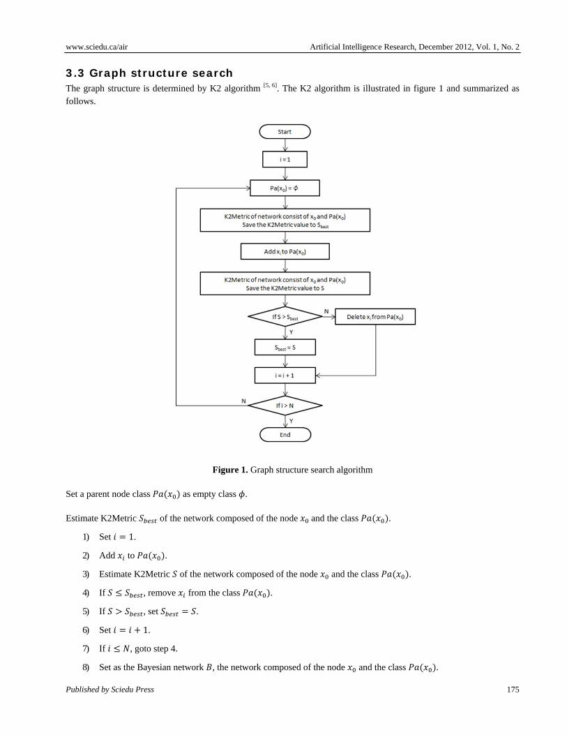
3.3 Graph structure search The graph structure is determined by K2 algorithm [5, 6]. The K2 algorithm is illustrated in figure 1 and summarized as follows.

Figure 1. Graph structure search algorithm

Set a parent node class as empty class .

Estimate K2Metric of the network composed of the node and the class .

1) Set 1.

2) Add to .

3) Estimate K2Metric of the network composed of the node and the class .

4) If , remove from the class .

5) If , set .

6) Set 1.

7) If , goto step 4.

8) Set as the Bayesian network , the network composed of the node and the class .


ISSN 1927-6974 E-ISSN 1927-6982 176

3.4 Probabilistic reasoning When the evidence of the random variable is given, the probability | is estimated by the marginalization algorithm with the conditional probability table [12].

The marginalization algorithm gives the probability | as follows.

| ∑ , ∑ ,⋯, ,⋯, ,∑ ∑ ,⋯, , (21)

where the notation ∑ denotes the summation over all states , , ⋯ , of the random variable .

4 Previous prediction algorithm

4.1 Process The process of the previous prediction algorithm is summarized as follows.

1) Transform stock price return into the discrete values set by Ward method.

2) Determine the Bayesian network from the discrete values set.

3) Predict the stock price by using the network .

4.2 Ward method Ward method determines the clusters so as to minimize the Euclid distances from samples to the cluster centers are

minimized. The notation , and denote the sample, the cluster and its center, respectively. The estimator is given as

, ⋃ (22)

C ∑ ,∈ (23)

where the notation , denotes the Euclid distance between and .

In the previous study [5], the Ward method and the uniform clustering were compared and then, the results show that the accuracy of Ward method was better than that of the uniform clustering. Therefore, Ward method is employed as the clustering algorithm.

4.3 Discretization of stock price return Stock price return is defined as [1, 2]:

ln ln 100 (24)

where the variable denotes the closing stock price on the day [9].

In the Bayesian network, random variables are specified at nodes. The use of Ward method, which is one of clustering algorithms, transforms the return into the set of discrete values. In this study, the Ward method is adopted as the clustering algorithm.



The set of the discrete values is defined as

, , ⋯ , (25)

where the notation and denote the discrete value and its total number, respectively.

The parameter is determined so as to minimize AIC which is defined as

AIC ln (26)

where the notation denotes the variance and the variable is the total number of nodes. The variance is defined as

∑ (27)

where 10 and the parameter denotes the actual stock price return.

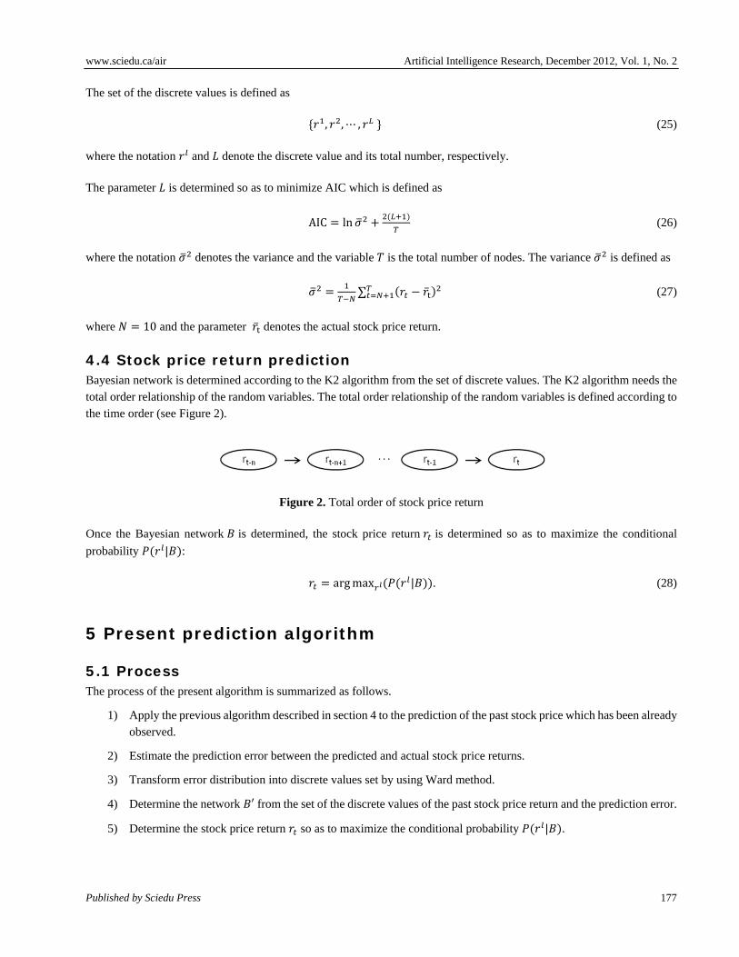
4.4 Stock price return prediction Bayesian network is determined according to the K2 algorithm from the set of discrete values. The K2 algorithm needs the total order relationship of the random variables. The total order relationship of the random variables is defined according to the time order (see Figure 2).

Figure 2. Total order of stock price return

Once the Bayesian network is determined, the stock price return is determined so as to maximize the conditional

probability | :

argmax | . (28)

5 Present prediction algorithm

5.1 Process The process of the present algorithm is summarized as follows.

1) Apply the previous algorithm described in section 4 to the prediction of the past stock price which has been already observed.

2) Estimate the prediction error between the predicted and actual stock price returns.

3) Transform error distribution into discrete values set by using Ward method.

4) Determine the network ′ from the set of the discrete values of the past stock price return and the prediction error.

5) Determine the stock price return so as to maximize the conditional probability | .


ISSN 1927-6974 E-ISSN 1927-6982 178

5.2 Discretization of prediction error When the past stock price is predicted by equation (28), a predicted and an actual stock prices are referred to as and , respectively. The prediction error is estimated by

. (29)

The use of Ward method transforms the error into the set of the discrete values which is defined as

, , ⋯ , (30)

where the notation and denote the discrete value and the total number of the discrete values, respectively.

The parameter is determined so as to minimize the AIC defined in equation (26).

5.3 Stock price return prediction The total order relationship of the random variables is shown in Figure 3.

Figure 3. Total order of stock price return and prediction error

Once the network is determined according to the algorithm in section 3, the stock price return is determined so as to

maximize the conditional probability | : argmax | (31)

6 Numerical examples

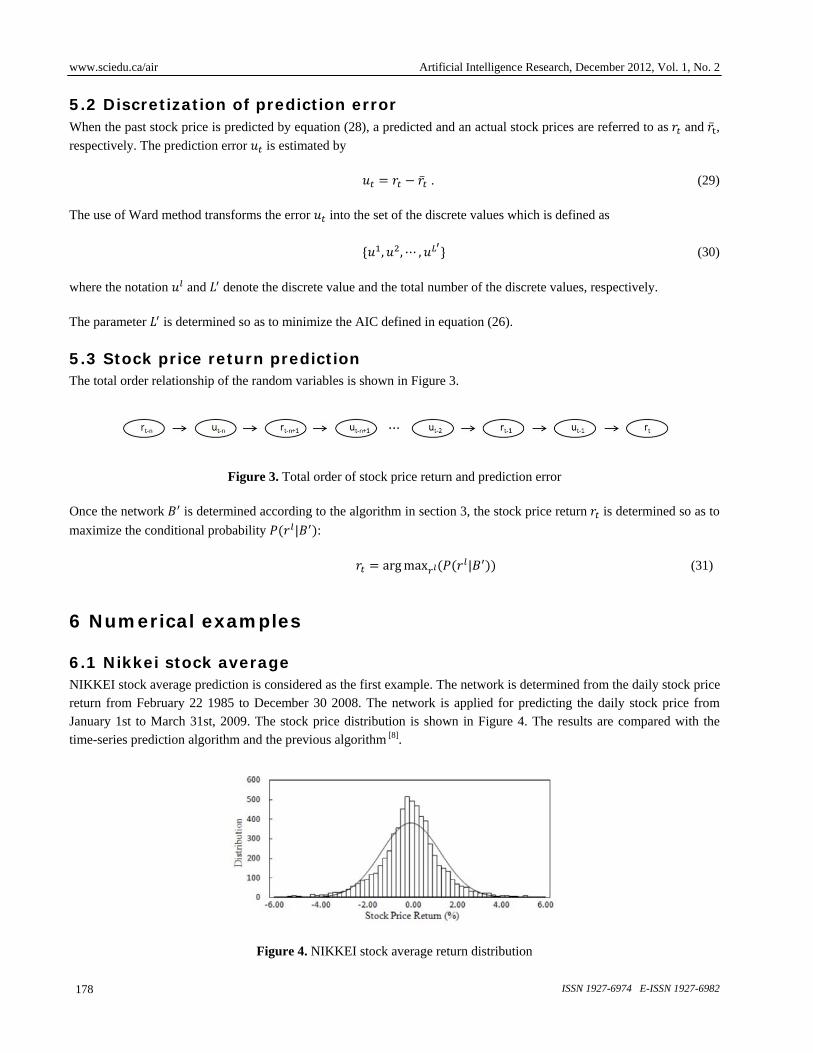
6.1 Nikkei stock average NIKKEI stock average prediction is considered as the first example. The network is determined from the daily stock price return from February 22 1985 to December 30 2008. The network is applied for predicting the daily stock price from January 1st to March 31st, 2009. The stock price distribution is shown in Figure 4. The results are compared with the time-series prediction algorithm and the previous algorithm [8].

Figure 4. NIKKEI stock average return distribution



6.1.1 Network determination Firstly, the network is determined from the stock price return alone. The effect of the number of discrete values to the AIC

of the network is compared in Table 1. The AIC is defined in equation (24). We notice that the AIC is smallest at 6. The

discrete values and the cluster parameters at 6 are listed in Table 2. The notation means the cluster center, which

is considered as the discrete value. The notation and denote the minimum and the maximum values of the

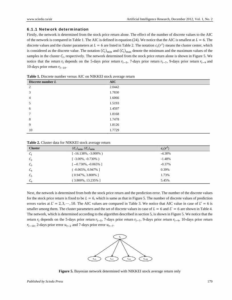
samples in the cluster , respectively. The network determined from the stock price return alone is shown in Figure 5. We

notice that the return depends on the 5-days prior return , 7-days prior return , 9-days prior return and

10-days prior return .

Table 1. Discrete number versus AIC on NIKKEI stock average return

Discrete number L AIC

2 2.0442

3 1.7830

4 1.6066

5 1.5193

6 1.4597

7 1.8168

8 1.7478

9 1.8126

10 1.7729

Table 2. Cluster data for NIKKEI stock average return

Cluster ,

[ -16.138%, -3.000% ) -4.30%

[ -3.00%, -0.730% ) -1.48%

[ --0.730%, -0.065% ] -0.37%

( -0.065%, 0.947% ] 0.39%

( 0.947%, 3.800% ] 1.73%

( 3.800%, 13.235% ] 5.45%

Next, the network is determined from both the stock price return and the prediction error. The number of the discrete values

for the stock price return is fixed to be 6, which is same as that in Figure 5. The number of discrete values of prediction

errors varies at 2, 3,⋯ , 10. The AIC values are compared in Table 3. We notice that AIC value in case of 6 is

smaller among them. The cluster parameters and the set of discrete values in case of 6 and 6 are shown in Table 4. The network, which is determined according to the algorithm described in section 5, is shown in Figure 5. We notice that the

return depends on the 5-days prior return , 7-days prior return , 9-days prior return , 10-days prior return

, 2-days prior error and 7-days prior error .

Figure 5. Bayesian network determined with NIKKEI stock average return only


ISSN 1927-6974 E-ISSN 1927-6982 180

Table 3. Discrete number versus AIC on prediction error of NIKKEI stock average return

Discrete number L’ AIC

2 1.6659

3 1.4587

4 1.5764

5 1.5132

6 1.3203

7 1.4596

8 1.4599

9 1.4602

10 1.4606

Table 4. Cluster data for prediction error of NIKKEI stock average return

Cluster ,

[ -16.67%, -2.87% ) -4.13%

[ -2.87%, -0.92% ) -1.59%

[ --0.92%, 0.00% ] -0.47%

( 0.00%, 1.40% ] 0.55%

( 1.40%, 3.71% ] 2.26%

( 3.71%, 16.74% ] 5.33%

6.1.2 Prediction accuracy The prediction accuracy is compared in Table 5. The labels AR(2), MA(2), ARMA(2,2) and ARCH(2,9) denote AR model

with 2, MA model with 2, ARMA model with 2 and 2, and ARCH model with 2 and 9, respectively. The labels BN(Previous) and BN(Present) denote the results by using Figure 5 and 6, respectively. The label “Maximum error”, “Minimum error”, “Average error”, and “Correlation coefficient” denote maximum daily error, minimum daily error, average value of daily errors, and the correlative coefficient, respectively. The correlative coefficient is estimated from the sets of the actual and the predicted stock prices. We notice from table 5 that the present method shows the largest correlative coefficient and smallest average and maximum errors among them. The average and maximum errors of the present method are 6% and 15% below them of the time-series prediction algorithms, respectively.

Table 5. Comparison of predicted and actual stock prices (NIKKEI stock average)

Model Maximum error Minimum error Average error Correlation coefficient

AR(2) 5.7648 0.0604 0.9278 2.4923 MA(2) 5.7746 0.0758 0.9276 2.4953 ARMA(2,2) 5.9389 0.0076 0.9250 2.5150 ARCH(2,9) 5.8342 0.0178 0.9268 2.5116 BN(Previous) 6.2948 0.0057 0.9099 2.9905 BN(Present) 4.9016 0.0105 0.9375 2.3467

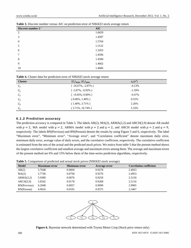
Figure 6. Bayesian network determined with Toyota Motor Corp (Stock price return only)



6.1.3 CPU time The present algorithm is compared with the previous algorithm using Bayesian network in their CPU times. The results are shown in Table 6. The labels BN (Previous) and BN(Present) denote the results by using Figures 4 and 5, respectively. The labels “Network Search” and “Prediction” denote the CPU times for determining Bayesian network and stock price return prediction, respectively. In the CPU time for determining Bayesian network, the present algorithm takes longer time than the previous algorithm by almost 70%. We notice that, in the present algorithm, the CPU time for determining Bayesian network is relatively expensive. The CPU time for predicting the stock price return, however, is much smaller than that for determining Bayesian network. We can conclude that, even if the network is determined in advance, the CPU cost for the stock price prediction is not expensive.

Table 6. Comparison of calculation cost of previous and present models

Network Search Prediction

BN(Previous) 529sec 0.691sec BN(Present) 908sec 0.887sec

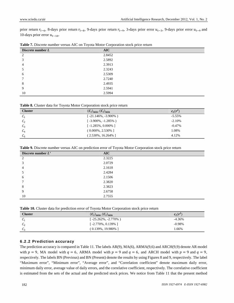
6.2 Toyota motor corporation The next example is the stock price of Toyota Motor Corporation. The stock price distribution is shown in Figure 7. We notice the distribution is a little far from the normal probability distribution. The network is determined from the daily stock price from February 22nd 1985 to December 30th 2008. Comparing Figures 4 and 7 reveals that the distribution in Figure 7 is multi-modal and thus, different from the normal distribution. The network is applied for predicting the daily stock price from January 1st to March 31st, 2009.

Figure 7. Toyota Motor Corporation stock price return distribution

6.2.1 Network determination The network is determined from the daily stock price alone. The total number of the discrete values varies at 2,3,⋯ ,10.

The AICs of the networks are listed in Table 7. We notice that the AIC is smallest at 5. The set of the discrete values at 5 is shown in Table 8. The network, which is determined according to the algorithm of section 4, is shown in Fig.8. We

notice that the return depends on the 1-days prior return , 4-days prior return , 6-days prior return , 8-days

prior return , and 9-days prior return .

Next, the network is determined from both the stock price return and the prediction error. The number of the discrete values

for the stock price return is fixed to be 5.

The number of discrete values of prediction errors is taken as 2,3,⋯ ,10. The AIC values are compared in Table 9. We

notice that AIC in case of 3 is smaller among them. The cluster parameters and the set of discrete values in case of 5 and 3 are shown in Table 10. The network, which is determined according to the algorithm described in section

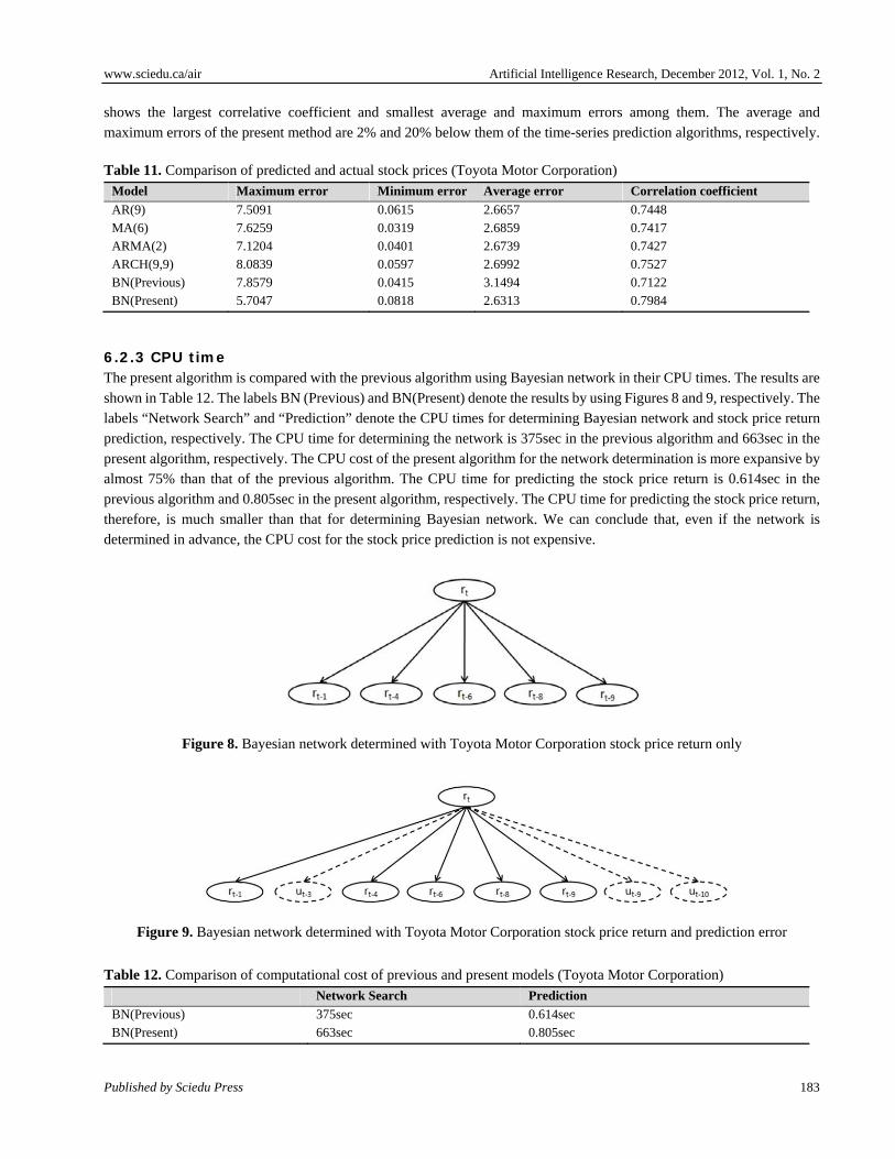
5, is shown in Figure 9. We notice that the return depends on the 1-day prior return , 4-days prior return , 6-days


ISSN 1927-6974 E-ISSN 1927-6982 182

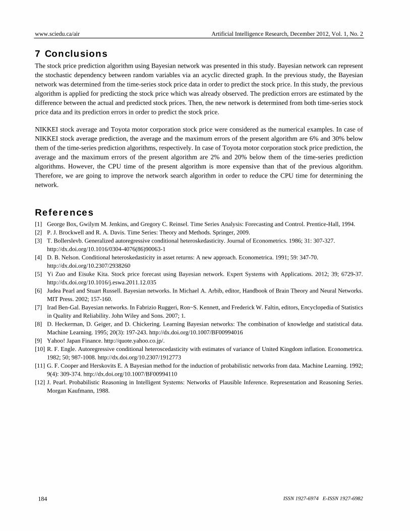
prior return , 8-days prior return , 9-days prior return , 3-days prior error , 9-days prior error and

10-days prior error .

Table 7. Discrete number versus AIC on Toyota Motor Corporation stock price return

Discrete number L AIC

2 2.8452 3 2.5892 4 2.3913 5 2.3243 6 2.5309 7 2.7240 8 2.4935 9 2.5941 10 2.5994

Table 8. Cluster data for Toyota Motor Corporation stock price return

Cluster ,

[ -21.146%, -3.900% ) -5.55%

[ -3.900%, -1.285% ) -2.10%

[ -1.285%, 0.000% ] -0.47%

( 0.000%, 2.530% ] 1.08%

( 2.530%, 16.264% ] 4.12%

Table 9. Discrete number versus AIC on prediction error of Toyota Motor Corporation stock price return

Discrete number L’ AIC

2 2.3225 3 2.0729 4 2.1618 5 2.4284 6 2.1506 7 2.3820 8 2.3823 9 2.6758 10 2.7555

Table 10. Cluster data for prediction error of Toyota Motor Corporation stock price return

Cluster ,

[ -25.262%, -2.770% ) -4.36%

[ -2.770%, 0.139% ] -0.98%

( 0.139%, 19.980% ] 1.66%

6.2.2 Prediction accuracy The prediction accuracy is compared in Table 11. The labels AR(9), MA(6), ARMA(9,6) and ARCH(9,9) denote AR model

with 9, MA model with 6, ARMA model with 9 and 6, and ARCH model with 9 and 9, respectively. The labels BN (Previous) and BN (Present) denote the results by using Figures 8 and 9, respectively. The label “Maximum error”, “Minimum error”, “Average error”, and “Correlation coefficient” denote maximum daily error, minimum daily error, average value of daily errors, and the correlative coefficient, respectively. The correlative coefficient is estimated from the sets of the actual and the predicted stock prices. We notice from Table 11 that the present method



shows the largest correlative coefficient and smallest average and maximum errors among them. The average and maximum errors of the present method are 2% and 20% below them of the time-series prediction algorithms, respectively.

Table 11. Comparison of predicted and actual stock prices (Toyota Motor Corporation)

Model Maximum error Minimum error Average error Correlation coefficient

AR(9) 7.5091 0.0615 2.6657 0.7448 MA(6) 7.6259 0.0319 2.6859 0.7417 ARMA(2) 7.1204 0.0401 2.6739 0.7427 ARCH(9,9) 8.0839 0.0597 2.6992 0.7527 BN(Previous) 7.8579 0.0415 3.1494 0.7122 BN(Present) 5.7047 0.0818 2.6313 0.7984

6.2.3 CPU time The present algorithm is compared with the previous algorithm using Bayesian network in their CPU times. The results are shown in Table 12. The labels BN (Previous) and BN(Present) denote the results by using Figures 8 and 9, respectively. The labels “Network Search” and “Prediction” denote the CPU times for determining Bayesian network and stock price return prediction, respectively. The CPU time for determining the network is 375sec in the previous algorithm and 663sec in the present algorithm, respectively. The CPU cost of the present algorithm for the network determination is more expansive by almost 75% than that of the previous algorithm. The CPU time for predicting the stock price return is 0.614sec in the previous algorithm and 0.805sec in the present algorithm, respectively. The CPU time for predicting the stock price return, therefore, is much smaller than that for determining Bayesian network. We can conclude that, even if the network is determined in advance, the CPU cost for the stock price prediction is not expensive.

Figure 8. Bayesian network determined with Toyota Motor Corporation stock price return only

Figure 9. Bayesian network determined with Toyota Motor Corporation stock price return and prediction error

Table 12. Comparison of computational cost of previous and present models (Toyota Motor Corporation)

Network Search Prediction

BN(Previous) 375sec 0.614sec BN(Present) 663sec 0.805sec


ISSN 1927-6974 E-ISSN 1927-6982 184

7 Conclusions The stock price prediction algorithm using Bayesian network was presented in this study. Bayesian network can represent the stochastic dependency between random variables via an acyclic directed graph. In the previous study, the Bayesian network was determined from the time-series stock price data in order to predict the stock price. In this study, the previous algorithm is applied for predicting the stock price which was already observed. The prediction errors are estimated by the difference between the actual and predicted stock prices. Then, the new network is determined from both time-series stock price data and its prediction errors in order to predict the stock price.

NIKKEI stock average and Toyota motor corporation stock price were considered as the numerical examples. In case of NIKKEI stock average prediction, the average and the maximum errors of the present algorithm are 6% and 30% below them of the time-series prediction algorithms, respectively. In case of Toyota motor corporation stock price prediction, the average and the maximum errors of the present algorithm are 2% and 20% below them of the time-series prediction algorithms. However, the CPU time of the present algorithm is more expensive than that of the previous algorithm. Therefore, we are going to improve the network search algorithm in order to reduce the CPU time for determining the network.

References [1] George Box, Gwilym M. Jenkins, and Gregory C. Reinsel. Time Series Analysis: Forecasting and Control. Prentice-Hall, 1994. [2] P. J. Brockwell and R. A. Davis. Time Series: Theory and Methods. Springer, 2009. [3] T. Bollerslevb. Generalized autoregressive conditional heteroskedasticity. Journal of Econometrics. 1986; 31: 307-327.

http://dx.doi.org/10.1016/0304-4076(86)90063-1 [4] D. B. Nelson. Conditional heteroskedasticity in asset returns: A new approach. Econometrica. 1991; 59: 347-70.

http://dx.doi.org/10.2307/2938260 [5] Yi Zuo and Eisuke Kita. Stock price forecast using Bayesian network. Expert Systems with Applications. 2012; 39; 6729-37.

http://dx.doi.org/10.1016/j.eswa.2011.12.035 [6] Judea Pearl and Stuart Russell. Bayesian networks. In Michael A. Arbib, editor, Handbook of Brain Theory and Neural Networks.

MIT Press. 2002; 157-160. [7] Irad Ben-Gal. Bayesian networks. In Fabrizio Ruggeri, Ron~S. Kennett, and Frederick W. Faltin, editors, Encyclopedia of Statistics

in Quality and Reliability. John Wiley and Sons. 2007; 1. [8] D. Heckerman, D. Geiger, and D. Chickering. Learning Bayesian networks: The combination of knowledge and statistical data.

Machine Learning. 1995; 20(3): 197-243. http://dx.doi.org/10.1007/BF00994016 [9] Yahoo! Japan Finance. http://quote.yahoo.co.jp/. [10] R. F. Engle. Autoregressive conditional heteroscedasticity with estimates of variance of United Kingdom inflation. Econometrica.

1982; 50; 987-1008. http://dx.doi.org/10.2307/1912773 [11] G. F. Cooper and Herskovits E. A Bayesian method for the induction of probabilistic networks from data. Machine Learning. 1992;

9(4): 309-374. http://dx.doi.org/10.1007/BF00994110 [12] J. Pearl. Probabilistic Reasoning in Intelligent Systems: Networks of Plausible Inference. Representation and Reasoning Series.

Morgan Kaufmann, 1988.

application of bayesian network to stock price prediction

Documents