NASA-TP-3441 19940017310

NASATechnicalPaper3441

December 1993

Application Guide forUniversal Source Encodingfor Space

Pen-Shu Yeh and Warner H. Miller

t • : . _ : ;=

ii

' i]

! "7 :ER

..... j

-"-'-:" --" L_-: :.2.: .-." .i-:.2 ':.,:2: ; j:":::-.-.

https://ntrs.nasa.gov/search.jsp?R=19940017310 2018-06-18T16:49:15+00:00Z

.I

llll_iiiiiiiilljf_3 1176 01409 5195

NASATechnicalPaper3441

1993

Application Guide forUniversal Source Encodingfor Space

Pen-Shu Yeh andWarner H. Miller

Goddard Space Flight CenterGreenbelt, Maryland

National AeronauticsandSpace Administration

Scientific and TechnicalInformation Branch

ABSTRACT

Lossless data compression has been studied for many NASA missions. The Rice algorithm hasbeen demonstrated to provide better performance than other available techniques on most scien-tific data. A top-level description of the Rice algorithm is first given, along with some new capa-bilities implemented in both software and hardware forms. The document then addresses systemsissues important for onboard implementation including sensor calibration, error propagation anddata packetization. The latter part of the guide provides twelve case study examples drawn from abroad spectrum of science instruments.

°°o111

ACKNOWLEDGEMENT

The authors wish to thank the following colleagues for providing technical information or data onthe science instruments used in case study examples. Some also gave valuable comments whichgreatly improve the content and readability of the document.

John BarkerGorden Chin

Davila JosephLarry Evans (with CSC)Keith Feggans (with ACC)Robert Griswold (with GST, Inc.)David Hancock, 3rdJim IronsKeith Lai (with HSTX)Tom Lynch (with Hughes)Ronald MullerRobert Rice (with JPL)Keith Strong (with Lockheed Palo Alto Research Lab.)Leslie ThompsonPaul Westmeyer

iv

TABLE OF CONTENTS

1.0 Introduction .............................................................................................................. 1

2.0 Algorithm ................................................................................................................. 2

2.1 The Preprocessor ................................................................................................................. 32.1.1 Predictor ................................................................................................................ 32.1.2 References............................................................................................................. 42.1.3 The Mapper ........................................................................................................... 4

2.2 Entropy Coder ..................................................................................................................... 42.2.1 The Sample-Split Options..................................................................................... 42.2.2 Option Selection ................................................................................................... 52.2.3 Low Entropy Option ............................................................................................. 52.2.4 Default Option ...................................................................................................... 5

3.0 Systems Issues ......................................................................................................... 5

3.1 Sensor Characteristics and Calibration ............................................................................... 5

3.2 Error Propagation ................................................................................................................ 6

3.3 Data Packetization and Compression Performance ............................................................ 7

4.0 Compression Illustrations ........................................................................................ 8

4.1 Landsat Thematic Mapper................................................................................................... 9

4.2 Heat Capacity Mapping Radiometer on Heat Capacity Mapping Mission ......................... 94.3 Moderate-Resolution Imaging Spectrometer (MODIS) on EOS ...................................... 12

4.4 Advanced Solid-State Array Spectrometer (ASAS) on C-130B ....................................... 12

4.5 NS001 Multispectral Scanner on C-130B ......................................................................... 15

4.6 Wide-Field Planetary Camera (WFPC) on Hubble Space Telescope ............................... 174.7 Soft X-ray Telescope (SXT) on Solar-A Mission ............................................................. 20

4.8 Goddard High-Resolution Spectrometer (GHRS) on HST............................................... 20

4.9 Acousto-Optical Spectrometer (AOS) on Submillimeter Wave Astronomy Satellite(SWAS).............................................................................................................................. 23

4.10 Gamma-Ray Spectrometer on Mars Observer .................................................................. 244.11 Radar Altimeter on TOPEX/POSEIDON ......................................................................... 26

4.12 Gas Chromatograph-Mass Spectrometer on Cassini......................................................... 28

5.0 References ..............................................................................................................29

Application Guide for Universal Source

Encoding for Space

1.0 Introduction

Lossless data compression has been suggested for many NASA applications to eitherincrease the science returnor to reduce the requirement on onboard memory, station con-tact time, and data archival volume. This type of compression technique guarantees a fullreconstruction of the original data without incurring any distortion in the process.

Of the many available lossless data compression algorithms, the Rice algorithm has beendemonstrated to perform better in most studies on scientific data. The algorithm has alsobeen implemented in a number of NASA's science exploration missions. The earlier appli-cations implemented the algorithm in software form executed by an onboard microproces-sor. In 1991, a hardware engineering model was built in an Application Specific IntegratedCircuit (ASIC) for proof of concept. This particular chip set was named as UniversalSource Encoder/Universal Source Decoder (USE/USD). Later, it was redesigned with sev-eral additional capabilities and implemented in Very Large Scale Integration (VLSI) cir-cuits using gate arrays suitable for space missions. The flight circuit is referred to asUniversal Source Encoder for Space (USES).

This document aims to provide first a top-level description of the Rice algorithm architec-ture, along with some new capabilities. It then addresses systems issues important foronboard implementation. It also aims to serve as an application guide. The latterpart ofthe document provides case study examples drawn from a broad spectrum of scienceinstruments. The examples demonstrate how to obtain optimal compression performancefor various scientific space applications. Some of these studies have resulted in an onboardimplementation; others provided input for future missions.

In the case study examples, whenever feasible, a compression performance comparisonwith another commercially available technique is included. No attempt was made toexhaust all existing techniques for this purpose. It should be noted that there may exist dif-ferent means to apply the Rice algorithm to the data, mainly, in preprocessing or reformat-ting the data before presenting it to the entropy coding module. The users should be awarethat the entropy coding scheme in the Rice algorithm, as discussed in reference 2, is a sub-set of Huffman codes optimal for Laplacian symbol sets. This set of Huffman codes alsoperforms well on Gaussian or Poisson symbol sets. To optimize performance, one wouldtry to preprocess the data set so that it conforms closely to a Laplacian symbol set distribu-tion. The technique for approaching this goal is only limited by the user's imagination.

The types of scientific instruments studied include Charge Coupled Device (CCD) imager,radio wave spectrometer, radar altimeter, gamma ray spectrometer and others. Only mis-

1

sion and instrument titles will be listed in this document; details on each mission andinstrument are not provided.

Users should consult the references for further information on the algorithm and relatedissues. Reference 1 provides a general overview of the Rice algorithm. Reference 2 detailsperformance analysis. An analysis on the requirement for data flow smoothing buffer isgiven in reference 3. Reference 4 describes the USE/USD VLSI hardware. Reference 5provides available hardware specification, while reference 6 provides a source for soft-ware code. The data structure standardized by the international space committee Consulta-tive Committee for Space Data Systems (CCSDS) is given in reference 7.

2.0 Algorithm

A block diagram of the architecture of the Rice algorithm is given in Figure 2.1. It consistsof a preprocessor to decorrelate data samples and subsequently map them into symbolssuitable for the following stage of entropy coding. The entropy coding module is a collec-tion of options operating in parallel over a large entropy range. The option yielding theleast number of coding bits will be selected. This selection is performed over a block of Jsamples to achieve adaptability to scene statistics. An Identification 0D) bit pattern is usedto identify the option selected for each block of J input data.

i ..................................... '

I"putD -IIP di°°rI Io.co eworq

Preprocessor

__ OptionSelect ID• I

Entropy Coder

Figure 2.1. The encoder architecture.

2

2.1 The Preprocessor

2.1.1 Predictor

Lossless source coding for data compression is a method by which only redundancy isremoved from the source data in order to achieve the objective that the reconstructed datais identical to the input data, or in other words, the combined pry- and postprocessor pro-cedure has to be completely reversible. There are many types of pre/postprocessors thathave this reversible property.

The decorrelation function of the preprocessor can be implemented by a judicious choiceof the predictor for an expected set of data samples. The decision should take into accountpossible variations in the background noise and the gain of the sensors for acquiring thedata. The predictor should be chosen to minimize the randomness of the noise resultingfrom the sensor nonuniformity. An optimal predictor would give small prediction errorswith a probability distribution resembling a Laplacian function. There are also some datatypes that require no decorrelation. These types can be routed directly to the entropy cod-ing module.

A technique widely used as a basic lossless preprocessor function is predictive coding.The simplest predictive coder is a unit-delay predictor shown in Figure 2.2. The output,A i, will be the difference between the input data symbol and the preceding data symbol.The input data signal is assumed to be already linearly quantized. The inherent compres-sion ability of such a predictive coder occurs typically from there being statistically fewerquantization levels used after the differencing operation than in the original input datasamples.

o

[

: Predictor

i! . _=_1,_2,...,_iX = X1,X2.... 'Xi _i . X_._+,_,_,). Mapper _---

i!iii_ii_iiiiiiiiiiiiiiiiil.._.Xiiiiii!E._o_iDelay I -1_ i .. i

A=A1,A2,...,A i

Figure 2.2. A unit-delay predictive preprocessor.

Several other types of prediction modes exist in the USES implementation. These include:

1. a default predictor that takes the previous data sample as the predictor value for thecurrent data sample.

2. an external predictor supplied by the user.

3. a 2D predictor that uses the average of the previous adjacent sample and a user-supplied value as the predictor value.

4. a multispectral (multi-source) predictor which uses data from one channel as input to ahigher-order prediction function for the data in a second channel.

These prediction modes are user-selectable during the initialization period for using thehardware. For software implementation, users can easily program any prediction schemethat best decorrelates the input data stream. Users would subsequently select the predic-tion mode as a run-time parameter.

2.1.2 References

A reference symbol is an unaltered data symbol upon which succeeding symbol differ-ences are based. References are required by the decoder to recover the absolute valuesfrom difference values except when the source encoder is operating in the entropy codingmode in which no prediction on data will be performed. The user must determine howoften to insert references. When inserted, the reference shall precede the first symbol of ablock of J symbols. In packetized formats, the reference shall be applied to the first samplein the packet data fields.

2.1.3 The Mapper

The function of the predictive coder is to decorrelate the incoming data stream by takingthe difference between data symbols. The mapper takes these difference values, both posi-tive and negative, and orders them, based on predictive values, sequentially as positive

integers. The mapper shall map the positive differences, Ai, into even _ii, and the negativedifferences into odd 5 i. For N-bit quantization, the mapped symbol set shall have 2 ele-ments 50, _il,..., _n (n = 2N -1). These elements preferably shall have corresponding prob-abilities approximating the following relationship:

P0 >-P1 > P2 > ... >-Pn,

where Pi is the probability of occurrence for symbol _ii.

2.2 Entropy Coder

2.2.1 The Sample-Split Options

The sample-split option in the Rice algorithm takes a block of J preprocessed data sam-ples, splits off the k least significant bits, and codes the remaining higher order bits with asimple comma code before appending the split-off bits to the coded data stream. Eachsample-split option in the Rice algorithm is optimal in an entropy range about one bit/sam-ple; only the one yielding the least amount of coding bits will be chosen and identified fora J-sample data block by the option select logic. This assures that the block will be codedwith one of the available Huffman codes, whose performance is better than other available

4

options on the same block of data. The k = 0 option is optimal in the entropy range of 1.5 -2.5 bit/sample; the k = 1 option is optimal in the range of 2.5 - 3.5 bit/sample, and so on forother k values. For the developed ASIC hardware that implements the split sample up to k= 12, the effective range for this scheme extends from 1.5 bit/sample to 14.5 bit/sample.The users should be made aware that the "entropy" is the information rate for an idealLaplacian symbol set, and usually can be approximated by the entropy of the predictionerrors from an actual data source.

2.2.2 Option Selection

The entropy coder includes a code-word selection, which selects the option that performsbest on the current block of symbols. The selection is made on the basis of the number ofbits that the selected parameter will use to code the current block of symbols. An identifierspecifies which of the optional parameters was used to code the accompanying set of codewords.

2.2.3 Low Entropy Option

The low entropy option implemented in the hardware extends the performance below 1.5bit/sample. When the prediction error comprises only small values, this low entropyoption can be very effective. The special case of a block of J errors of zero prediction val-ues is also handled in this option by specifying only an ID code. This mode is especiallyuseful for compressing thresholded imagery.

2.2.4 Default Option

The option, not to apply any parameter, is the default case. If it is the selected option, thepreprocessed block of symbols is passed through the encoder process without alterationbut with an appended identifier.

3.0 Systems Issues

Several systems issues related to embedding data compression scheme onboard a space-craft should be addressed. These include the relation between the focal-plane arrayarrangement and the data sampling/prediction direction, the subsequent data packetizingscheme and how it relates to error propagation in case of bit error incurred in the commu-nication channel, and the amount of smoothing buffer required when the compressed datais passed to a constant-rate communication link without prior buffering.

3.1 Sensor Characteristics and Calibration

Advanced imaging instruments and spectrometers often use arrays of individual detectorsarranged in a 1D or 2D configuration; one example is the Charge Coupled Device (CCD).These individual detectors tend to have slight differences in response to the same inputphoton intensity. For instance, CCDs usually have a different gain and dark current value

for each individual detector element. It is important to have the sensor well calibrated sothat the data reflects the actual signals received by the sensor. Simulations have shown thatfor CCD types of sensors, gain and dark current variations as small as 0.2% of the fulldynamic range can render the prediction scheme less effective for data compression.Besides calibration, in order to maximize the compression gain, the prediction schemeused in the preprocessor in Figure 2.1 will be much more effective when data acquired onone detector element is used as the predictor for data acquired on the same detector whosecharacteristics are stationary, in general, over the data collection period. An example is thepush-broom scheme used in many Earth-viewing satellite systems depicted in Figure 3.1.An array of detectors is arranged in the cross-track direction, which also is the detectordata readout direction. The scanning of the ground scene is achieved by the motion of thesatellite in the along-track direction. In such configuration, predictive coding will be mosteffective in the along-track direction, in which data from the same detector is used as thepredictor. An example of how to optimize compression performance in the presence ofdetector nonuniformity is given in Section 4.4.

Pi Pi+1 DataReadout1

Along- /Track l DetectorArrayDirectionI

Cross-TrackDirection

Figure 3.1. Push-broom scanning scheme.

3.2 Error Propagation

User acceptability to distortion resulting from channel bit errors is mission-dependent, andis strongly a function of received Signal-to-Noise-Ratio (SNR), the data format, the errordetection and correction technique and the percent of distorted data that is tolerable. Amajor concern in using data compression is the possibility of error propagation in theevent of a single bit error in the compressed data stream. During the decompression pro-cess, a single bit error can lead to a reconstruction error over extended runs of data points.There are two general approaches to minimizing such effect. First, it is important to have aclean channel for data communication. Some form of error detection/correction scheme is

recommended for compressed data. Second, packetization of compressed data in a properformat in conjunction with the error control coding, will prevent error propagation into thenext packet. An example for space application is to packetize the compressed data of onescanline in a CCSDS recommended data packet format (reference 7) and the compresseddata of the next scanline into a second packet. In case of a bit error in one packet, the

decompression error will only propagate to the end of the packet, providing that the com-pression/decompression algorithm does not depend on information from a second packet.

3.3 Data Packetization and Compression Performance

The total number of coding bits resulting from losslessly compressing a fixed number ofdata samples is usually a variable. The CCSDS data architecture provides a structure topacketize the variable length data stream into a packet, which then can be put into a fixedlength frame. Packetization is essential for preventing error propagation as mentioned ear-lier; it also can impact the compression performance for the data set. The Rice algorithmand the low-entropy option process a block of data of a predetermined number of samples,typically 8, 16, 24, etc., at one time. To facilitate decoding, packetization should beformed on compressed data of multiple blocks of as short as one block of samples or aslong as the user desires. However, to prevent error propagation in the event of bit error, areasonable length of data blocks will be chosen for a packet. The compression perform-ance is optimal for every block of samples and is not dependent on the packet length.

There exist other available compression algorithms whose performance depends on estab-lishing the long-term statistics of the samples in a file. In general such schemes will givegood compression performance for a large file and poor performance for a relativelysmaller file. And if packetization, as a means of preventing error propagation, is used inconjunction with these algorithms, one would expect poor performance for a shorterpacket and a better performance for a larger packet. The drawback is that the loss of datacaused by error propagation may be intolerable for the larger packet.

An example of how a data packetization scheme affects compression performance, as acomparison between the current technique and a known technique, is given in Section 4.6.

An alternative to using a variable-length packet is to fix the length of the packet. Fixed-length packets typically will have compressed data followed by fill bits to bring the packetto a fixed length. If the compressed-bit count is greater than the fixed length, truncationoccurs with loss of data. The decoder recognizes the truncation condition and signalswhen a block has been truncated by outputting dummy symbols. The decoder will outputas many dummy symbols as would be in a typical packet that was not truncated. If one ormore blocks were truncated, corresponding blocks of dummy symbols will be outputted tofill out the required blocks-per-packet.

Depending on the mission requirement, the variable-length packets resulting from packingthe compressed bit stream into CCSDS packets can be stored in a large onboard memoryor multiplexed with other data packets before being stored in the memory device. In thiscase, the large-capacity memory device will smooth out the variation in the packet length.Subsequent readout from the memory will be performed at a fixed rate. In other situations,the variable-length packets may have to be temporarily buffered before a direct transmis-sion to the communication link. The temporary buffer serves as a smoothing buffer for thelink. Occasionally fill bits are inserted in the data stream to provide a constant readoutrate. The amount of buffer needed is a variable of the incoming packet rate, the packet

length statistics, and the readout rate. An analysis on the buffer requirement is given in ref-erence 3.

4.0 Compression Illustrations

This section contains compression study results for several different instruments. Thecompression performance is expressed as Compression Ratio (CR). It is defined as the

ratio of the quantization level in bits to the average code word length, also in bits. When

necessary, the performance of the enhanced Rice algorithm is compared with the com-monly known and commercially available Lample-Ziv-Welch (LZW) algorithm. The

LZW algorithm is particularly efficient in compressing text file that has grammatical struc-ture. It is available on most Unix machines as a system utility. All the studies were per-formed in software simulator implemented in language C on a Sun Sparc workstation.

Twelve examples are included in this document. Table 4.0 summarizes the result. Noticethat the compression ratio is instrument data dependent. For a specific instrument type, the

compression ratio can vary from one test data set to the next. The readers should refer to

each individual example for more details on each study.

Table 4.0. Summary of Compression Ratio

USES

Instrument Compression Ratio

Thematic Mapper 1.83

Heat Capacity 2.19

Mapping Radiometer

Moderate-Resolution 1.89/bandl

Imaging Spectrometer 1.37/band2

Advanced Solid-State 1.74/broad band

Array Spectrometer

NS001 Multispectral 1.60/avergedover

Scanner 8 bands

Wide-Field Planetary 2.97/no thresholdCamera

Soft X-ray Telescope 4.96

Goddard High- 1.72/spectrum onlyResolution Spectrometer

Acousto-Optical 2.3

Spectrometer

Gamma-ray Spectrome- 26/at 5-sec collec-ter tion

Radar Altimeter 1.41

Gas Chromatograph- 1.94

Mass Spectrometer

8

4.1 Landsat Thematic Mapper

Mission Purpose: The Landsat program was initiated for the study of Earth's surface andresources. Landsat-1, Landsat-2, and Landsat-3 were launched between 1972 and 1978.Landsat-4 was launched in 1982, and Landsat-5 in 1984.

Landsat Thematic Mapper (TM) on Landsat-4, 5, and 6: The TM data represent typi-cal land observation data acquired by projecting mirror-scanned imagery to solid-statedetectors. The sensor for band 1-5 is a staggered 16-element photo-diode array; it is a stag-gered 4-element array for band 6. An image acquired on Landsat-4 at 30m ground resolu-tion for band 1 in the wavelength region of 0.45 - 0.52 _m is shown in Figure 4.1. This 8-bit 512x512 image was taken over Sierra Nevada in California and has relatively highinformation over the mountainous area.

Compression Study: Using a 1D predictor in the horizontal direction, setting a block sizeof 16 samples and inserting one reference per every image line, the lossless compressiongives a compression ratio at 1.83 for the 8-bit image. In contrast, a direct application of theLZW algorithm, available on Unix system as compress, gives a compression ratio at 1.51.

4.2 Heat Capacity Mapping Radiometer on Heat Capacity MappingMission

Mission Purpose: Launched in 1978, the mission supported exploratory scientific investi-gations to establish the feasibility of utilizing thermal infrared remote sensor-derived tem-perature measurements of the Earth's surface within a 12-hour interval, and to apply thenight/day temperature difference measurements to the determination of thermal inertia ofEarth's surface.

Heat Capacity Mapping Radiometer: The sensor is a solid state photo-detector sensitivein either the visible or the infrared region. A typical 8-bit image taken in the visible lightregion is given in Figure 4.2, at a ground resolution of 500m over the Chesapeake Bayarea on the East Coast.

Compression Study:

Prediction on 1D: Choosing 1D default prediction in the horizontal direction, and settingblock size J at 16, lossless compression gives a compression ratio of 2.19. A direct appli-cation of Unix compress gives a compression ratio of 1.95.

Prediction on 2D: Using a 2D predictor that takes the average of the previous sample andthe sample on the previous scan line, and keeping other parameters the same, USES com-pression gives a CR of 2.28, about 5% increase from using a 1D predictor.

Figure 4.1. Thematic mapper image.

10

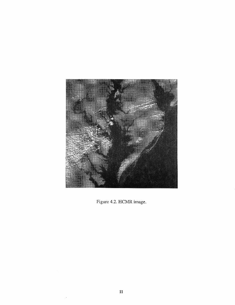
Figure 4.2. HCMR image.

11

4.3 Moderate-Resolution Imaging Spectrometer (MODIS) on EOS

Mission Purpose: MODIS is one of the instruments planned for the Earth Observing Sys-tem (EOS). The EOS mission is commissioned to study the global change of the Earthover a prolonged period of time through various sensors for detecting changes in theEarth's environment.

Moderate-Resolution Imaging Spectrometer: The spectrometer has 36 bands over thevisible and infrared wavelength region. The sensor uses monolithic focal-plane CCD orphoto-diode arrays of sizes 10, 20, or 40 elements designated for different bands. A simu-lated image at 250m resolution over eastern Florida is given in Figure 4.3 for band 1 cen-tered at 0.659 ktm and band 2 centered at 0.865 [.tm. MODIS will generate data at a 12-bitdynamic range. This test image size is 256x256.

Compression Study:

Prediction on 1D: Using 1D default prediction in the horizontal direction, and at a blocksize J of 16, USES compression gives a compression ratio of 1.89 for band 1 test image,and a ratio of 1.56 for band 2. The Unix compress gives a ratio of 1.71 for band 1 and 1.37for band 2 test image.

Multispectral prediction: Using band 1 as input to the higher order predictor for band 2,and keeping other parameters the same as in 1D prediction, the compression ratioincreases from 1.56 to 1.67, a 7% increase in this case. The efficiency of the multispectralprediction technique will be further explored later.

4.4 Advanced Solid-State Array Spectrometer (ASAS) on C-130B

Mission Purpose: The NASA Earth Resources Aircraft Program at Ames Research Cen-ter operates a C-130B aircraft to acquire data for earth science research. It provides a plat-form for a variety of sensors that collect data in support of scientific projects sponsored byNASA, as well as federal, state, university, and industry investigators.

Advanced Solid-State Array Spectrometer (ASAS): The sensor collects data at 10-bitdynamic range, with 29 or more spatially registered bands. The image in Figure 4.4 wasacquired for the geologic remote-sensing field experiment. It's ground resolution is 5.5macross track and the size of the image is 512x360. Images from several bands are com-bined to give a broader bandwidth of 500-870nm to simulate a possible panchromaticband for the Landsat-7 program. It is evident from the image that, because of either detec-tor nonuniformity or insufficient calibration, streaking noise appears across the image inthe vertical direction.

Compression Study:

Prediction in horizontal direction: This prediction scheme does not try to optimize the pre-dictor performance. The compression ratio is 1.42 using 10-bit as base in calculating theratio. On computer systems, these types of 10-bit/pixel data are often stored as integer*2data using two bytes for each datum, the algorithm will compress the file at a ratio of 2.27,compared to 1.58 achieved by the Unix compress utility.

Prediction in vertical direction: To reduce the prediction error, a more preferable predictorapplies the prediction on data from the same detector. The compression ratio nowincreases from 1.42 to 1.74 and the file size reduction ratio improves to 2.78.

12

Figure 4.3. MODIS test image.

13

Figure 4.4. ASAS image.

14

4.5 NS001 Multispectral Scanner on C-130BMission Purpose: Same as Section 4.4.

NS001 Multispectral Scanner: The scanner contains the seven Landsat-4 ThematicMapper bands plus a band from 1.13 to 1.35 ]Am.The specific bands are as follows:

Table 4.5.1. NS001 Bands

Band SpectralBandwidth,]Am1 0A58 -0.519

2 0.529-0.603

3 0.633-0.697

4 0.767-0.910

5 1.13- 1.35

6 1.57- 1.71

7 2.10- 2.38

8 10.9- 12.3

An 8-band image acquired at ground resolution of 2.36m was first low-pass filtered toobtain a ground resolution at approximately 4.72m. This set of images was subsampled2:1 and displayed in Figure 4.5. The image was taken over Mountain View and Moffetfield in California. The compression study, however, was performed on the 4.72m image.The image has an 8-bit dynamic range.

Compression Study:

In-band prediction: Selecting the block size to be 16, the lossless compression within eachband of this set of images gives the performance listed in Table 4.5.2 under USES (in-band). The within-band predictor used is the 1D previous pixel within each horizontalline. For comparison purposes, the performance obtained by the Unix compress is alsogiven.

Cross-band prediction: When adjacent band is used as a predictor in the multispectralmode of the lossless compression technique, the performance improvement is obvious, asshown in the same table under USES (cross-band). In this study, band 1 is used as the pre-dictor for band 2, band 2 is used as the predictor for band 3, etc. The users should be madeaware that this study only suggests which band is more compressible with additionalinformation from the other bands. It is evident that for the particular urban scene in Figure4.5, band 5 and band 7 can acquire substantial improvement in reducing the data volume,while bands 2, 3, 4, and 6 receive moderate improvement. For the far infrared band 8, thestudy shows it is more effective to use only in-band compression.

15

Figure 4.5. NS001 multispectral image.

16

Table 4.5.2. Compression Ratio on TM Test Data

UNIX USES USES % CR

Band compress (in-band) (cross-band) Increase

1 1.04 1A0 / /2 1.06 1.36 1.57 15.4%

3 1.10 1.46 1.66 13.7%

4 1.09 1.43 1.51 5.6%5 1.07 1.42 1.90 33.8%

6 1.11 1.45 1.58 9.0%

7 1.08 1.44 1.80 25.0%

8 1.08 1.43 1.36 -4.9%

4.6 Wide-Field Planetary Camera (WFPC) on Hubble Space Telescope

Mission Purpose: The Hubble Space Telescope (HST), launched in 1990, is aimed atacquiring astronomy data at a resolution never achieved before and observing objects thatare 100 times fainter than other observatories have observed.

Wide-Field Planetary Camera (WFPC): The camera uses four area array CCD detec-tors. A typical star field observed by this camera is shown in Figure 4.6. This particularimage data has maximum value of a 12-bit dynamic range, yet the background minimumvalue is of 9-bit value.

Compression Study: Two studies are performed:

Threshold Study: The effect of thresholding a star field on the compression performance isexplored in this study. Different threshold values will be applied to this image, and the val-ues of the data will be clipped at the threshold when they are smaller than the thresholdvalues. The thresholding operation does not change the visual quality of the image. All thebright stars are unaffected. The resultant image will be compressed losslessly and thecompression will make use of the low-entropy option frequently over the image. The orig-inal image in Figure 4.6 has a minimum quantized value of 423 and an array size of800x800. The compression was performed using a block size of 16 and a default predictorin the horizontal line direction. Results are summarized in the following table.

Table 4.6.1. Compression Ratio at Different Threshold Values

ThresholdValues USES LZW

None 2.97 3.30

430 2.99 3.33

440 11.92 17.15

450 41.20 63.53

460 53.52 91.48

470 63.66 110.73

17

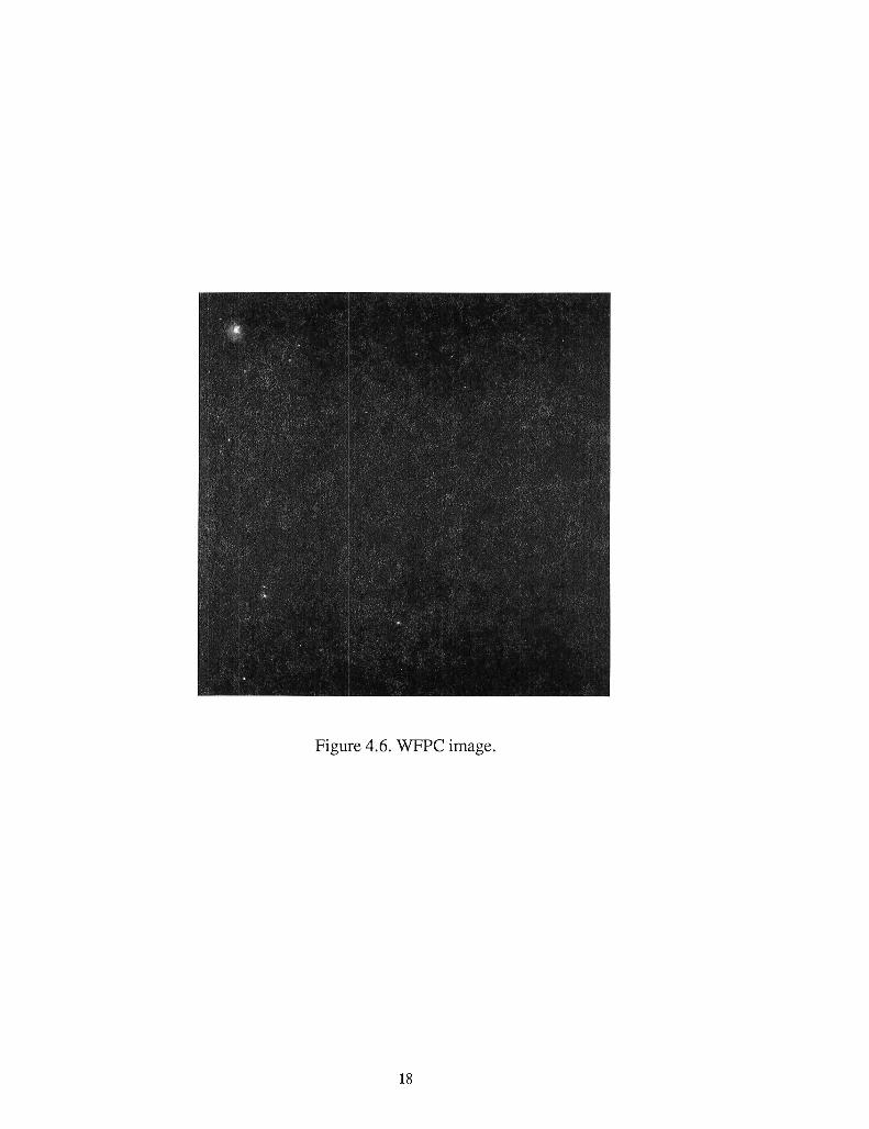
Figure 4.6. WFPC image.

18

These results are also compared with those obtained using the Unix compress command.One notices that the performance of the LZW algorithm over the whole image is betterthan that of USES. However, after considering the error propagation and packetizationissues involved in implementing a lossless algorithm, the results are reversed.

Packetization Study: When a packet data format is used for the compressed data, it isexpected that during decompression, the reconstruction error caused by a single bit errorin the packet will not propagate to the next packet. It implies that the data packets are inde-pendent of each other, that no code tables or statistics of data is passed from one packet tothe next. To explore the effect of packet size on the compression performance, severalindividual lines from Figure 4.6 are extracted and compressed separately. The results inTable 4.6.2 are obtained on lines 101 through 104, which cover partially the brightest starcluster on the upper left comer of Figure 4.6.

Table 4.6.2. Compression Ratio vs. Packet Size

Packet Size,Threshold No. of Lines USES LZW

None 1 (Line 101) 2.89 1.94

None I (Line 102) 2.90 1.92

None 1 (Line 103) 2.86 1.90

None 1 (Line 104) 2.88 1.90

None 2 (Line 101- 2.90 2.13102)

None 2 (Line 103- 2.87 2.09, 104)

None 4 (Line 101- 2.89 2.29104)

470 1 (Line 101) 16.24 6.98

470 1 (Line 102) 16.92 6.98

470 1 (Line 103) 15.42 6.94

470 1 (Line 104) 16.24 6.67

470 2 (Line 101- 16.45 8.70102)

470 2 (Line 103- 15.80 8.60104)

470 4 (Line 101- 16.06 10.30104)

19

4.7 Soft X-ray Telescope (SXT) on Solar-A Mission

Mission Purpose: The Solar-A mission, renamed as Yohkoh mission after its successfullaunch in August, 1991, is dedicated to the study of solar flares, especially of high-energyphenomena observed in the X- and gamma-ray ranges.

Soft X-ray Telescope (SXT): The instrument is a grazing-incidence reflecting telescopefor the detection of X-ray in the wavelength range of 3-60 Angstrom. It uses a 1024x1024CCD detector array to cover the whole Solar disk. Data acquired from the CCD is of 12-bit quantization and is processed on board to provide 8-bit telemetry data. The image inFigure 4.7 is an averaged image of size 512x512 with dynamic range up to 15 bits in float-ing point format as a result of further ground processing.

Compression Study: The test image is first rounded to the nearest integer. Then a 1Ddefault predictor is applied to this seemingly high-contrast image. A compression ratio of4.69 is achieved, which means that only 3.2 bits are needed per pixel to provide the fullprecision of this 15-bit image.

4.8 Goddard High-Resolution Spectrometer (GHRS) on HST

Mission Purpose: Same as Section 3.6.

Goddard High-Resolution Spectrometer (GHRS): The primary scientific objective ofthis instrument is to investigate the interstellar medium, stellar winds, evolution, andextra-galactic sources. Its sensors are two photo-diode arrays optimal in different wave-length regions, both in the UV range. Figure 4.8 gives examples of a typical spectrum anda background trace. These traces have 512 data values; each is capable of storing digitalcounts in a dynamic range of 107. Spectral shapes usually do not vary much. However,subtle variations of the spectrum in such large dynamic range presents a challenge for anylossless data compression algorithm. Two different prediction schemes are applied: thefirst uses the previous sample within the same trace, and the second uses the previous tracein the same category (spectrum or background) as a predictor. The results are summarizedbelow in Table 4.8. The test data set has data maximum value smaller than 16-bit dynamicrange, the compression ratio was thus calculated relative to 16 bits.

20

Figure 4.7. Solar-A X-ray image.

21

GHRS SPECTRUM

500040003000

20001000

........... , ......... , , ,

0 100 200 300 400 500 600

GHRS BACKGROUND8000 ................................

6000

4000

2000

i i i i |l i ,

0 100 200 300 400 500 600

Figure 4.8. GHRS data samples.

Table 4.8. Compression Ratio for GHRS

Trace Predictor USES LZW

spectrum 1 previous sample 1.64 <1.0

spectrum 2 previous sample 1.63 <1.0

spectrum 2 spectrum 1 1.72 NA

background 1 previous sample 2.51 1.63

background 2 previous sample 2.51 1.68

background 2 background 1 1.53 NA

22

4.9 Acousto-Optical Spectrometer (AOS) on Submillimeter WaveAstronomy Satellite (SWAS)

Mission Purpose: The Submillimeter Wave Astronomy Satellite (SWAS) is a SmallExplorer (SMEX) mission, scheduled for launch in the summer of 1995 aboard a Pegasuslauncher. The objective of the SWAS is to study the energy balance and physical condi-tions of the molecular clouds in the Galaxy by observing the radio-wave spectrum specificto certain molecules. It will relate these results to theories of star formation and planetary

systems. The SMEX platform ptovides relatively inexpensive and shorter developmenttime for the science'mission. SWAS is a pioneering mission that packages a completeradio astronomy observatory into a small payload.

Acousto-Optical Spectrometer: The AOS utilizes a Bragg cell to convert the radio fre-quency energy from the SWAS submillimeter receiver into an acoustic wave, which thendiffracts a laser beam onto a CCD array. The sensor has 1450 elements with 16-bit read-out. A typical spectrum is shown in Figure 4.9(a). An expanded view of a portion of twospectral traces is given in Figure 4.9(b). Because of the detector nonuniformity, the differ-ence in the Analog-to-Digital Converter (ADC) gain between even-odd channels, andeffects caused by temperature variations, the spectra have nonuniform offset valuesbetween traces, in addition to the saw-tooth-shaped variation between samples within atrace. Because of limited available onboard memory, a compression ratio of over 2:1 isrequired for this mission.

SWAS5.0x104

4.0xl 04 _

3.0x104

2.0x104

1.0x1040 , .

0 500 1000 1500(o). A typlcol spectrol troce

4.0x1043.8x104

3"6x104 _3.4×10 4

3.2xl 04 i3.0x104 , ,1100 1120 1140 1160 1180 1200

(b). Two troces exponded

Figure 4.9. AOS radio-wave spectrum.

23

Compression Study: The large dynamic range and the variations within each tracepresent a challenge to the compression algorithm. Default prediction between samples isineffective when the odd and even channels have different ADC gains. Three predictionmodes are studied; the results are given in Table 4.9.

Table 4.9 SWAS Compression Result

Predictor USES

previous sample 1.58

previous trace 1.61(external predictormode)

previoustrace 2.32(multispectralmode)

The result shows that even with the similarity in spectral traces, a predictor using an adja-cent trace in a direct manner will not improve the compression performance caused by theuneven background offset. The multispectral predictor mode is especially effective indealing with spatially registered multiple data sources with background offsets. In con-trast, the LZW compression on the same spectral trace achieves no compression.

4.10 Gamma-Ray Spectrometer on Mars Observer

Mission Purpose: The Mars Observer was launched in September 1992. The Observerwill collect data through several instruments to help the scientists understand the Martiansurface, atmospheric properties and the interactions between the various elementsinvolved.

Gamma-Ray Spectrometer (GRS): The spectrometer uses a high-purity germaniumdetector for gamma rays. The flight spectrum is collected over sixteen thousand channels,each corresponding to a gamma-ray energy range. The total energy range of a spectrumextends from 0.2 Mev to 10 Mev. Typical spectra for a 5-second and a 50-second collec-tion time are given in Figure 4.10.1. These spectra show the random nature of the count;some are actually zero over several bins. The spectral count dynamic range is 8-bit.

Compression Study: Two different schemes using the same compression algorithm havebeen simulated. One scheme applies the USES algorithm directly to the spectrum, and theother implements a two-layer coding structure.

Direct application of USES (one-pass scheme): In this single pass implementation, theblock size J is set at 16, and the entropy-coding mode is selected to bypass the predictorand the mapping function; the algorithm achieves over 20:1 lossless compression for a 5-second spectrum. As gamma-ray collection time increases, the achievable compressiondecreases

24

5 second spectrum8

6C

40

0

0 5.0x103 1.0x104 1.5×104 2.0x104chonnel

50 second spectrum8O

6O

e---_ 40OU

2oO ....... | _ ...................

m m A_

0 5.0x103 1.0x104 1.5x104 2.0x]04channel

Figure 4.10.1. Gamma-ray spectrum.

Two-layer scheme: In a two-layer scheme, two passes are needed to compress the data.

The first pass finds the channel numbers that have valid counts, and generates run-lengthof channels between them. Meanwhile, a count file is created which holds only the valid

counts as data in the file. In the second pass, both the channel run-length file and the count

file are compressed using the lossless compression algorithm at a block size of 16 and

using the 1D default prediction mode.

The results of both schemes are plotted in Figure 4.10.2 and compared to the projected

results from the actual implementation on the GRS instrument on the Mars Observer. The

actual implementation used a different layered structure to code the valid channels and

counts and also employed a different low-entropy coding option.

The GRS spectrum offers a specific example that requires an efficient source coding tech-

nique for low entropy data. For the 5-second spectrum, over 90% of the data are coded

with the low-entropy option.

25

Lossless compression using LZW algorithm on the gamma-ray spectrum data producescompression ratios slightly lower than those from the one-pass application of USES at alldifferent gamma-ray collection time.

_,,,_0 I I i !

__ 2-pass

._o 25 Implemented-_ 1-passorr 20 _"co

"_ 15

ffl "_.E 10 .... .-..._o

5 -

, , , I , , , I , , , I , , , ! , , ,

0 20 40 60 80 100collection time, second

Figure 4.10.2. Compression result on GRS data.

4.11 Radar Altimeter on TOPEX/POSEIDON

Mission Purpose: Launched in August 1992, the TOPEX/POSEIDON satellite will makethe most accurate measurements ever of the sea surface using the satellite's radar altime-ter, one of the six instruments on the spacecraft. The mission will help the scientists under-stand the interaction between ocean, atmosphere, and global climate.

Radar Altimeter: The dual-frequency radar altimeter measures the distance to the oceansurface by measuring the time it takes for a radar signal to reflect off the water surface andreturn to the spacecraft. Subsequent computations and corrections permit determination ofthe sea level to within an accuracy of a few centimeters. The altimeter data traces areinherently very noisy. A typical set of traces over water and land is given in Figure 4.11.These are all 8-bit data, with 64 samples for every trace.

26

_°°I

iiiI1501-

"100 1

Altimetertracesoverwater

300

25O

200

150

100

50

Altimetertracesoverland

Figure 4.11. Typical radar altimeter traces.

Compression Study: Lossless compression study was performed on these two data setsby setting a default prediction mode that uses the previous sample as predictor. The resultsare summarized in the following table:

27

Table 4.11. Compression Ratio for Altimeter Data

File USES LZW

water 1.43 1.08

land 1.40 < 1

Using a predictor across the trace does not provide consistent improvement over using thedefault predictor within trace.

4.12 Gas Chromatograph-Mass Spectrometer on Cassini

Mission Purpose: The Cassini mission includes a Saturn Orbiter and the Huygens Probewhich will descend into the atmosphere of Titan, one of Saturn's moons. The launch isscheduled for 1997 to allow a Saturn encounter in 2004. The objectives of this missioninclude more detailed studies of Saturn's atmosphere, rings, and magnetosphere, close-upstudies of Saturn's satellites, and investigations on Titan's atmosphere and surface.

Gas Chromatograph-Mass Spectrometer (GCMS): The instrument uses chromatogra-phy to separate gas molecules of different structures and the mass spectrometer to obtainmass distribution. Some typical GCMS traces are shown in Figure 4.12 in which the time-axis denotes different traces and the mass axis shows the mass distribution within a trace.

Onboard data integration and other processing may be needed for this instrument besidesdata compression. This particular test set has a dynamic range of 16 bits.

Compression Study: Simulation was performed with several different configurations.The first one uses a predictor in the same trace, that is, by using a mass channel as predic-tor for the next mass channel; the second uses a predictor across the trace. The latter casehas two data configurations for compression: when a block of 16 data is taken in the massdirection, then a buffer of one trace is needed to hold the previous trace as predictor for thenext trace; when a block of data is taken in the time direction, a buffer large enough tohold 16 traces is needed. The results obtained are tabulated in Table 4.12.

Table 4.12. Compression Ratio on GCMS Data

Predictor CompressionMode Direction USES

1D default mass axis 1.65

previous trace mass axis 1.93

previous trace time axis 1.96

Using LZW compression on the same file would achieve a compression ratio of 1.22.

28

8_104: -

Figure 4.12. Typical GCMS test data.

5.0 References

1. Rice, Robert E, Pen-Shu Yeh andWarner H. Miller', "Algorithms for a Very HighSpeed Universal Noiseless Coding Module," JPL Publication 91-1, 1991. A shortenedversion "Algorithms for High-Speed Universal Noiseless Coding," is published in theProceedings of the AIAA Computing in Aerospace 9 Conference, San Diego, CA, Oct.19-21, 1993.

2. Yeh, Pen-Shu, Robert E Rice and WarnerH. Miller, "On the Optimality of CodeOptions for a Universal Noiseless Coder," Revised version, JPL Publication 91-2,1991. A shortened version "On the Optimality of a Universal Noiseless Coder," is pub-lished in the Proceedings of the AJAA Computing in Aerospace 9 Conference, SanDiego, CA, Oct. 19-21, 1993.

3. Yeh, Pen-Shu, and Warner H. Miller, "The Implementation of A Lossless Data Com-pression Module in An Advanced Orbiting System: Issues And Tradeoffs," in Proceed-ings of the First ESA Workshop on Computer Vision and Image Processing for

29

Spaceborne Applications, ESTEC, Noordwijk, The Netherlands, June 10-12, 1991.Post-print available from the authors at Goddard Space Flight Center, Greenbelt, MD,20771, USA.

4. Venbrux, Jack, Pen-Shu Yeh and Muye N. Liu, "A VLSI Chip Set for High-SpeedLossless Data Compression," IEEE Trans. on Circuits and Systems for Video Technol-ogy, Vol. 2, No. 4, Dec. 1992.

5. "Universal Source Encoder- USE" Product Specification, Version 4.1, Microelectron-ics Research Center, University of New Mexico, 1991, and "Universal Source Encoderfor Space - USES," Preliminary Product Specification, Version 2.0, MRC, Universityof New Mexico, 1993.

6. Software simulator, available from the Microelectronics Research Center, University ofNew Mexico.

7. "Advanced Orbiting Systems: Networks and Data Links: Architectural Specification,"CCSDS 701.0-B-1 Blue Book, Oct. 1989.

30

Form Approved

REPORT DOCUMENTATION PAGE OMBNo.0704-0188PublicreportingburdenforthiscollectionofInformationisestimatedto average1 hourperresponse,includingthetimeforreviewinginstructions,searchingexistingdatasources,gatheringandmalntalnln@thedataneeded,andcompletingandreviewingthecollectionof information.Sendcommentsregardingthisburdenestimateoranyotheralpect ofthiscollectionof information,includingsuggestionsforreducingthisburden,toWashingtonHeadquartersServices,DirectorateforInformationOperationsandReports,1215JefferloflDavisHighway,Suite1204,Arlington,VA22202-4302,andtotheOfficeof ManagementandBudget,PaperworkReductionProject(0704-0188),Walhlngton,DC 20503.

1. AGENCY USE ONLY (Leave blank) 2. REPORT DATE 3. REPORT TYPE AND DATES COVERED

December 1993 Technical Paper4. TITLE AND SUBTITLE 5. FUNDING NUMBERS

Application Guide for Universal Source Encoding for Space 730310-20-46

6. AUTHOR(S)

Pen-Shu Yeh and Warner H. Miller

7. PERFORMING ORGANIZATION NAME(S) AND ADDRESS (ES) 8. PEFORMING ORGANIZATIONREPORT NUMBER

Goddard Space Flight CenterGreenbelt, Maryland 20771 94B00028

9. SPONSORING ! MONITORING ADGENCY NAME(S) AND ADDRESS (ES) 10. SPONSORING / MONITORINGADGENCY REPORT NUMBER

National Aeronautics and Space AdministrationWashington, DC 20546-0001 NASA TP-3441

11. SUPPLEM ENTARY NOTES

Yeh and Miller: NASA/GOddard Space Flight Center, Greenbelt, Maryland

12a. DISTRIBUTION / AVAILABILITY STATMENT 12b. DISTRIBUTION CODE

Unclassified - Unlimited

Subject Category 32

13. ABSTRACT (Maximum 200 words)

Lossless data compression has been studied for many NASA missions. The Rice algorithm has beendemonstrated to provide better performance than other available techniques on most scientific data. Atop-level description of the Rice algorithm is first given, along with some new capabilities implementedin both software and hardware forms. The document then addresses systems issues important foronboard implementation, including sensor calibration, error propagation, and data pecketization. Thelatter part of the guide provides twelve case study examples drawn from a broad spectrum of scienceinstruments.

14. SUBJECT TERMS 15. NUMBER OF PAGES

42Source coding, Universal source encoding, data compression 16.PRICECODE

17. SECURITY CLASSIRCATION 18. SECURITY CLASSIFICATION 19. SECURITY CLASSIFICATION 20. UMITATION OF ABSTRACT

OF REPORT OF THIS PAGE OF ABSTRACTUnclassified Unclassified Unclassified

NSN 7540-01-280-5500 Standard Form 298 (Rev. 2-89)PrescribedbyANSiStd.z3g.18298-102