Application and Science of Crash Reduction FactorsFun, fun, fun ‘till your daddy takes the T‐bird away

Larry Hagen, P.E., PTOE

Workshop Series

Today’s Presentation

Application and Science of Crash 

Reduction Factors

Wed. Oct. 30 Highway Safety Evaluation

Wed. Nov. 6 Highway Safety Manual

Wed. Nov. 13 Application and Science of Crash Reduction Factors

Wed. Nov. 20 Requirements for HSIP Applications

Wed. Dec 4 Safety Funding Categories/Requirements/Conditions

Wed. Dec. 11Is Your Project Feasible? What’s Next and How Do We Move Forward?

Wed. Dec. 18 B/C Calculations plus NPV Calculations – New WP Guidelines

2014

Wed. Jan. 8 Safety Projects & The Local Agency Program (LAP)

Wed. Jan. 15Development of the Safety/LAP Project Schedule for Funding Purposes

Wed. Jan. 22 Safety/LAP Project Development

Wed. Jan. 29 Key to Successful Safety Programs

U R HERE

What is a CRF?

A CRF is one of the many TLA’s that we use in traffic engineering.  Here are some others:

• ADT• HCM• HSM• MOE

TLA

Three Letter Acronym

What is a CRF?

A CRF is one of the many TLA’s that we use in traffic engineering.  Here are some others:

• ADT• HCM• HSM• MOE

ADT

Average Daily Traffic

HCM

Highway Capacity Manual

HSM

Highway Safety Manual

MOE

LarryCurly

Moe

MOE

Measure Of Effectiveness

CRF

Crash Reduction Factor

CRF is a MOE

The Crash Reduction Factor is a measure of how effective you are at reducing crashes.

CRF

Crash Reduction Factor

CMF

Crash Modification Factor

CRF vs CMF

CRFA  Crash Reduction Factor is an estimate of the percentage reduction in crashes due to a particular countermeasure.

CMFA Crash Modification Factor is a multiplicative factor used to compute the expected number of crashes after implementing a given countermeasure.

CRF vs CMF

CRF CMFRange of values ‐∞ < CRF < 1.0 0 < CMF < ∞No change in crashes 0 1.0

Eliminate all crashes 1.0 0

Double the number of crashes ‐1.0 2.0

Half the number of crashes 0.5 0.5

15% less crashes 0.15 0.85

15% more crashes ‐0.15 1.15

CRF = 1 ‐ CMFCMF = 1 ‐ CRF

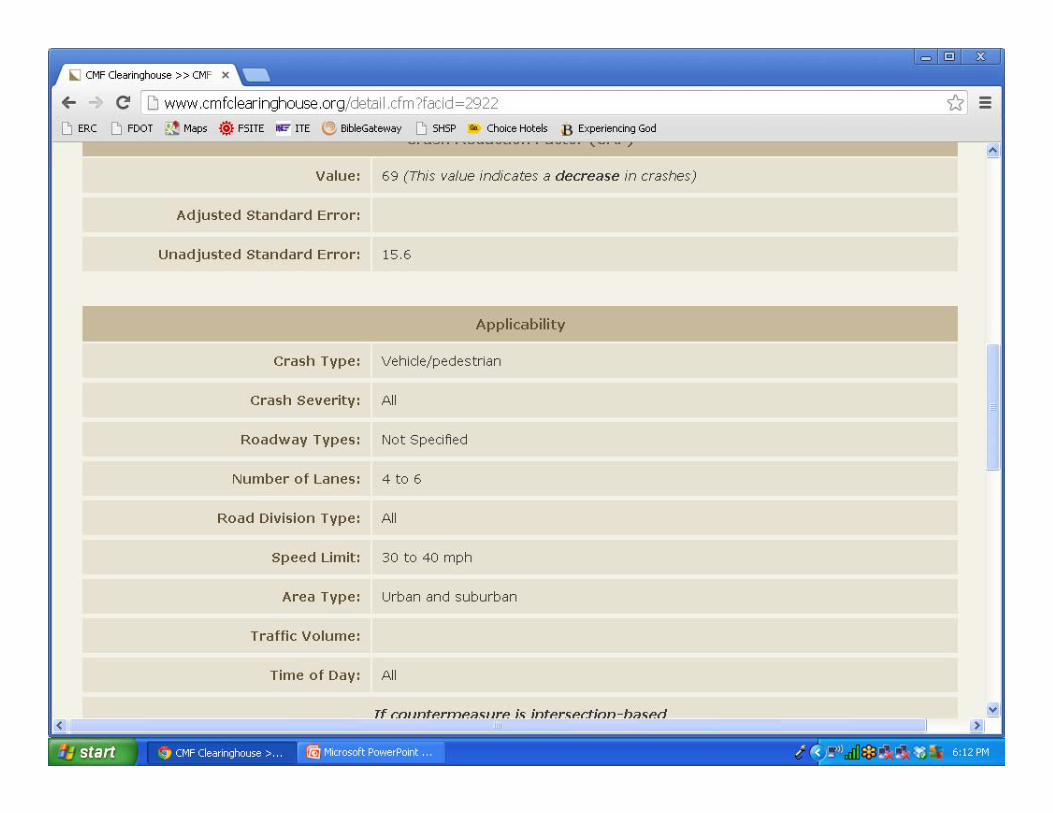
Where do I find CRF’s?

Florida DOT CRF’s

Highway Safety Manual

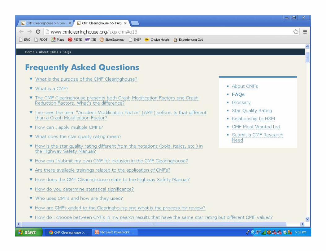
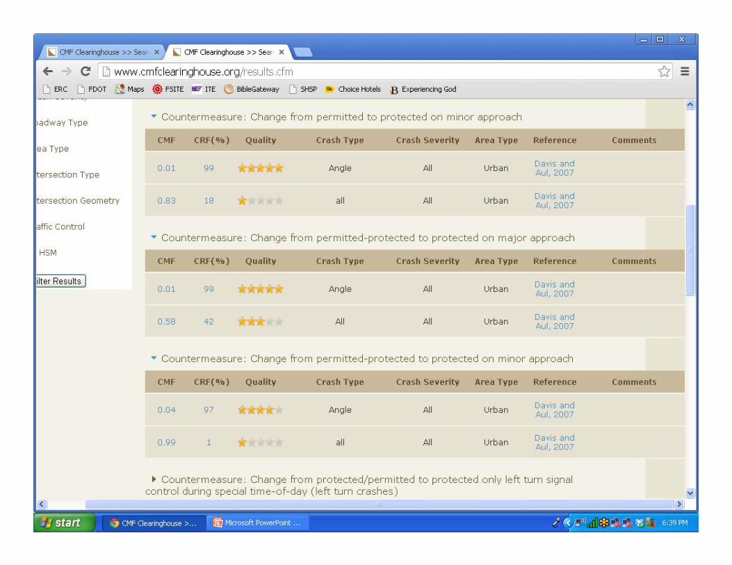
CMF Clearinghousewww.cmfclearinghouse.org

Florida DOT CRF’s

Crash Reduction Factors from studies in Florida

Produced by Lehman Center at FIU

Crash Reduction Analysis System Hub (CRASH)

Updated in 2005

Update to Peter Hsu’s work in graduate school at UF

Highway Safety Manual

Tables in the HSM contain CMF’s

Must convert to CRF’s if that is what you need

NOTE: there are separate CMF’s for the predictive models and for project analysis 

Typically, the CMF’s for the predictive models should NOT be used for other purposes and the other CMF’s should not be used with the predictive models

WARNING!ALWAYS use caution when looking up or applying CMF’s or CRF’s

HSM Predictive Models

Part C of the HSM

HSM Predictive Models

Safety Performance Function for facility type

Crash Modification Factors (Functions)

Calibration Factor

EB Adjustment

HSM Predictive Models

What are Safety Performance Functions?• Mathematical Regression Models for Roadway Segments and 

Intersections:• Developed from data for a number of similar sites• Developed for specific site types and “base conditions”• Function of only a few variables, primarily AADT• Used to calculate the expected crash frequency (crashes/year) for a 

set of base geometric and traffic control conditions Purpose of Crash Modification Factors• Adjusts the calculated SPF predicted value for base conditions to 

actual or proposed conditions• Accounts for the difference between base conditions and site specific 

conditions

HSM Predictive Models

Rural Two‐Lane Roadway Segments

SPF Prediction Model for Base Conditions:

Nspf‐rs = AADT x L x 365x10‐6 x e(‐0.312)

Nspf‐rs = predicted total crash frequency for roadway segment base conditions (crashes/year)

AADT = average annual daily traffic volume (vpd)

L = length of roadway segment (miles)

HSM Predictive ModelsBase Conditions for Rural Two‐Lane Roadway Segments:

Lane Width:  12 feet Shoulder Width:  6 feet Shoulder Type:  Paved Roadside Hazard Rating:         3 Driveway Density:   <5 driveways/mile Grade:  < 3% Horizontal Curvature:  None Vertical Curvature:  None Centerline rumble strips:        None TWLTL, climbing, or passing lanes:  None Lighting:  None Automated Speed Enforcement:       None

HSM Predictive Models

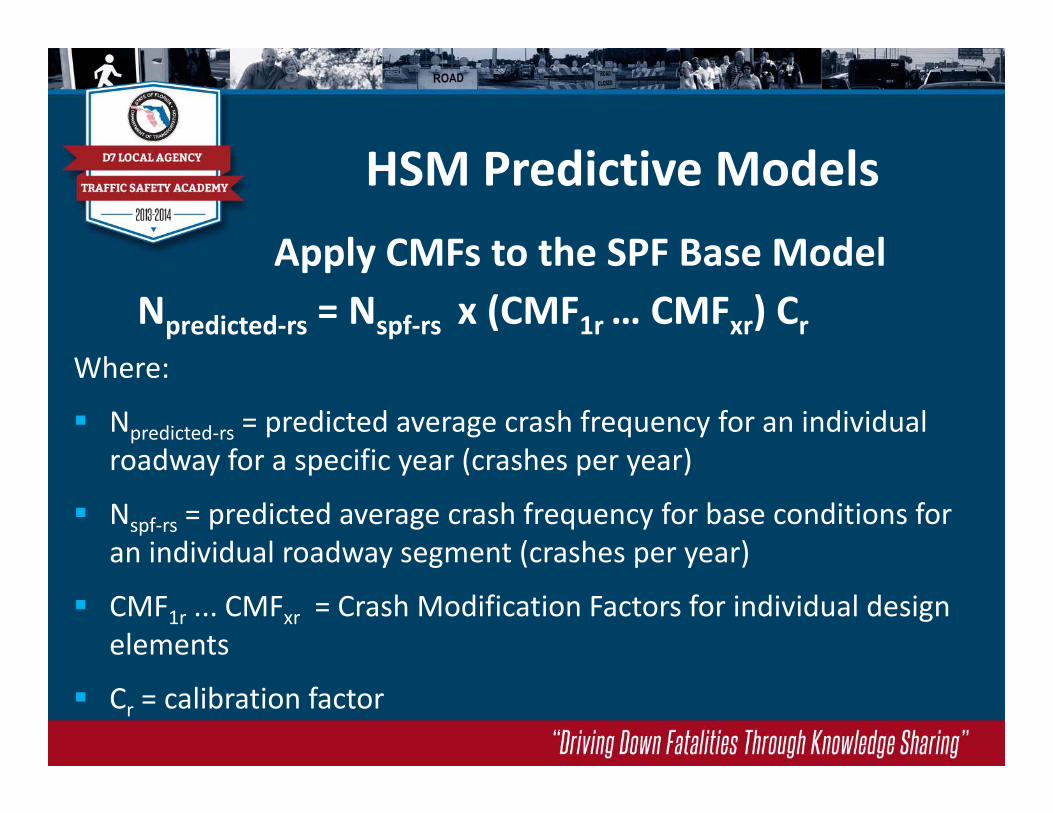
Npredicted‐rs = Nspf‐rs  x (CMF1r … CMFxr) Cr

Apply CMFs to the SPF Base Model

Where:

Npredicted‐rs = predicted average crash frequency for an individual roadway for a specific year (crashes per year)

Nspf‐rs = predicted average crash frequency for base conditions for an individual roadway segment (crashes per year)

CMF1r ... CMFxr = Crash Modification Factors for individual design elements

Cr = calibration factor

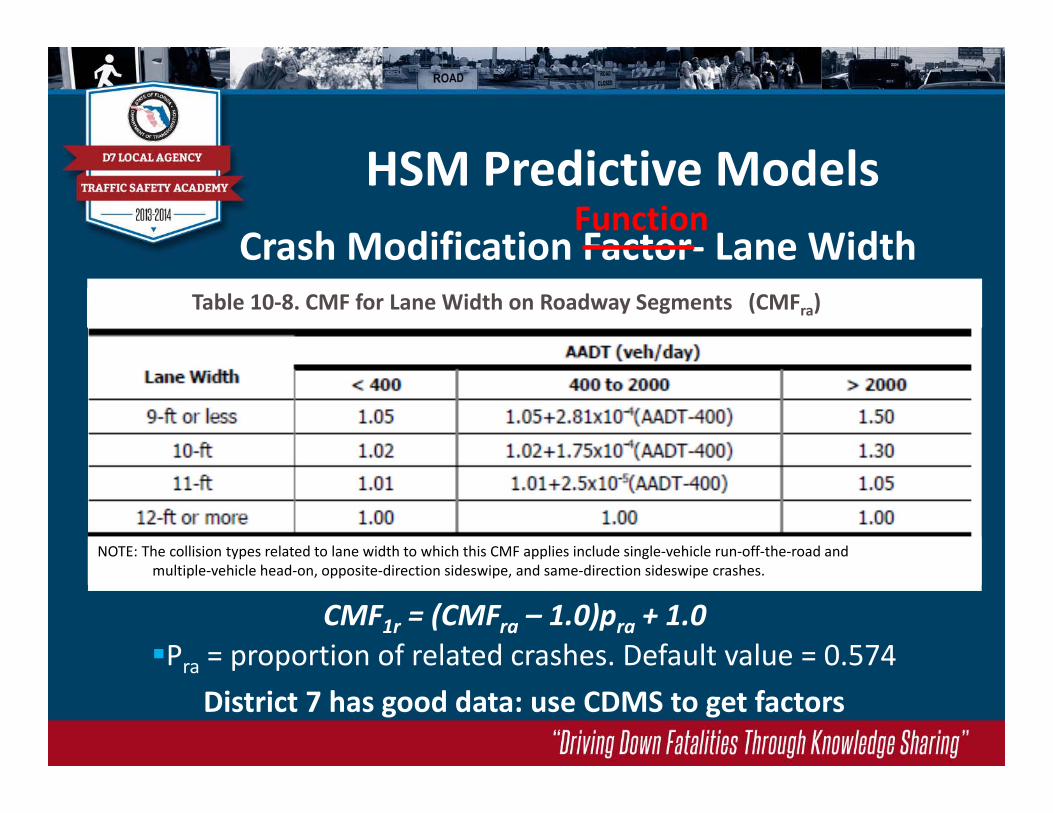
HSM Predictive ModelsCrash Modification Factor‐ Lane Width 

Pra = proportion of related crashes. Default value = 0.574 CMF1r = (CMFra – 1.0)pra + 1.0

District 7 has good data: use CDMS to get factors 

(CMFra)Table 10‐8. CMF for Lane Width on Roadway Segments

NOTE: The collision types related to lane width to which this CMF applies include single‐vehicle run‐off‐the‐road and multiple‐vehicle head‐on, opposite‐direction sideswipe, and same‐direction sideswipe crashes.

Function

WARNING!ALWAYS use caution when looking up or applying CMF’s or CRF’s

Table on the previous slide is ONLY applicable for use with the predictive model for rural two‐lane roadway segments! 

HSM Predictive Models

Multiplication of CMFs in Part C

In the Part C predictive method, an SPF estimate is multiplied by a series of CMFs to adjust the estimate of crash frequency from the base condition to the specific conditions present at a site. The CMFs are multiplicative because the effects of the features they represent are presumed to be independent. However, little research exists regarding the independence of these effects, but this is a reasonable assumption based on current knowledge. The use of observed crash frequency data in the EB Method can help to compensate for bias caused by lack of independence of the CMFs. As new research is completed, future HSM editions may be able to address the independence (or lack of independence) of these effects more fully.

HSM CMF’s

Multiplication of CMFs in Part DCMFs are also used in estimating the anticipated effects of proposed future treatments or countermeasures (e.g., in some of the methods discussed in Section C.8). The limited understanding of interrelationships between the various treatments presented in Part D requires consideration, especially when more than three CMFs are proposed. If CMFs are multiplied together, it is possible to overestimate the combined affect of multiple treatments when it is expected that more than one of the treatments may affect the same type of crash. The implementation of wider lanes and wider shoulders along a corridor is an example of a combined treatment where the independence of the individual treatments is unclear, because both treatments are expected to reduce the same crash types. When CMFs are multiplied, the practitioner accepts the assumption that the effects represented by the CMFs are independent of one another. Users should exercise engineering judgment to assess the interrelationship and/or independence of individual elements or treatments being considered for implementation.

HSM CMF’s

Compatibility of Multiple CMFs

Engineering judgment is also necessary in the use of combined CMFs where multiple treatments change the overall nature or character of the site; in this case, certain CMFs used in the analysis of the existing site conditions and the proposed treatment may not be compatible. An example of this concern is the installation of a roundabout at an urban two‐way stop‐controlled or signalized intersection. The procedure for estimating the crash frequency after installation of a roundabout (see Chapter 12) is to estimate the average crash frequency for the existing site conditions (as a SPF for roundabouts in currently unavailable) and then apply an CMF for a conventional intersection to roundabout conversion. Installing a roundabout changes the nature of the site so that other CMFs applicable to existing urban two‐way stop controlled or signalized intersections may no longer be relevant.

WARNING!ALWAYS use caution when looking up or applying CMF’s or CRF’s

You must use extreme care and caution when combining CMF’s! NEVER try to combine CRF’s! 

Combining CRFs

Just DON’T do it!

Certainly not additive

25% + 35% ≠ 60%for CRFs

Combining CRFs

Just DON’T do it!

Certainly not additive

Convert to CMFs

Multiply if applicable

Combining CMFs

Multiply if applicable

Consider independence

No more than three

Star Quality Rating

Relative Rating Excellent Fair Poor

Study Design

Statistically rigorous study design with reference group or randomized experiment and

control

Cross sectional study or other coefficient based analysis Simple before / after study

Sample Size Large sample, multiple years, diversity of sites

Moderate sample size, limited years, and limited diversity of

sitesLimited homogeneous sample

Standard Error Small compared to CRFRelatively large SE, but

confidence interval does not include zero

Large SE and confidence interval includes zero

Potential Bias Controls for all sources of known potential bias

Controls for some sources of potential bias

No consideration of potential bias

Data Source Diversity in States representing different geographies

Limited to one State, but diversity in geography within

State (e.g., CA)

Limited to one jurisdiction in one State

Submitted studies are ranked in the following categories: 

2 points 1 point 0 points

Star Quality Rating

Final quality rating is based on weighted score: 

Score = (2*study design) + (2*sample size) + standard error + potential bias + data source

Star rating based on the score

Score Star Rating

14 (max possible) 5 Stars

11 – 13 4 Stars

7 – 10 3 Stars

3 – 6 2 Stars

1 – 2 1 Star

0 0 Stars

Precision vs Accuracy

Accuracy & Precision?

Source: Figure 3B‐1 and Figure 10‐3 HSM

Study of Two‐Lane Rural Roads in Colorado

Example – Enhance delineation

2‐lane rural roadway, AADT = 16,000

Nighttime + wet‐weather crashes

County‐maintained roadway

Currently, no RPM’s

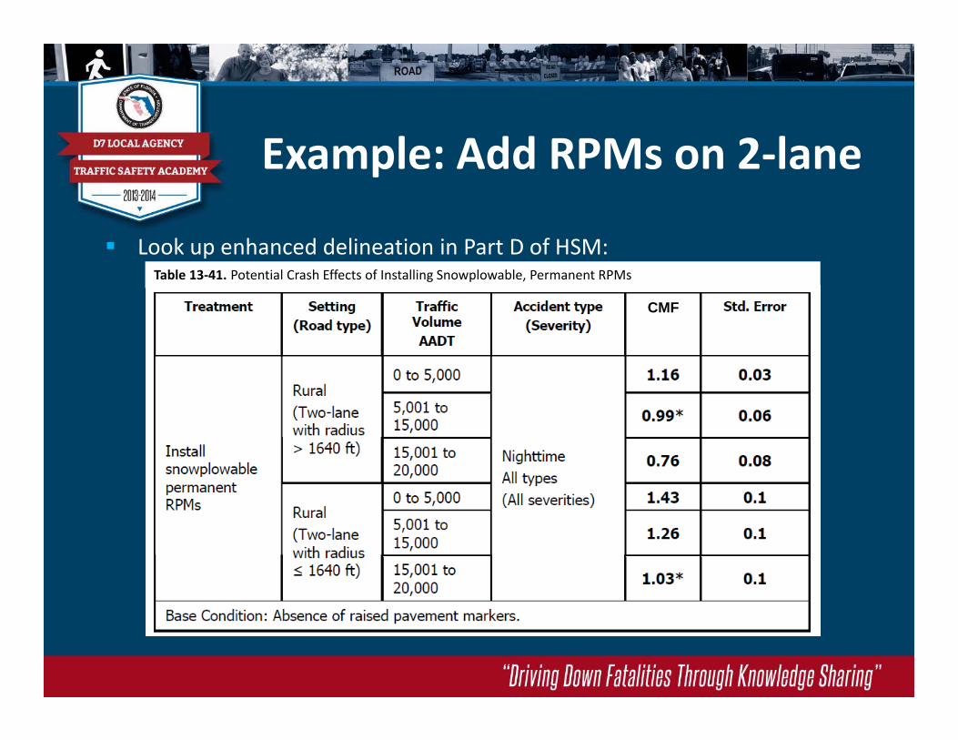
Example: Add RPMs on 2‐lane 

Look up enhanced delineation in Part D of HSM:

CMF

Table 13‐41. Potential Crash Effects of Installing Snowplowable, Permanent RPMs

WARNING!ALWAYS use caution when looking up or applying CMF’s or CRF’s

Is this applicable? 

Text in the HSM study clearly says “installation of snowplowable, permanent RPM’s”

But isn’t every RPM installed in Florida resistant to every snowplow typically used in Florida?  

Proceed with CAUTION!

Check the notes…

NOTE:  Bold text is used for the most reliable CMFs.  These CMFs have a standard error or 0.1 or less.

Example: Add RPMs on 2‐lane 

Look up enhanced delineation in Part D of HSM:

CMF

Table 13‐41. Potential Crash Effects of Installing Snowplowable, Permanent RPMs

Does this make sense?

Check the text…

The crash effects of installing snowplowable RPMs on low volume (AADT of 0 to 5,000), medium volume (AADT of 5,001 to 15,000), and high volume (AADT of 15,001 to 20,000) roads are shown in Table 13‐411  (2).  

The varying crash effect by traffic volume is likely due to the lower design standards (e.g., narrower lanes, narrower shoulders, etc.) associated with low volume roads (2). Providing improved delineation, such as RPMs, may cause drivers to increase their speeds. The varying crash effect by curve radius is likely related to the negative impact of speed increases (2). The base condition of the CMFs (i.e., the condition in which the CMF = 1.00) is the absence RPMs.

Example: Add RPMs on 2‐lane 

Look up enhanced delineation in Part D of HSM:

CMF

Table 13‐41. Potential Crash Effects of Installing Snowplowable, Permanent RPMs

Note which crash types this applies to

Example – Enhance delineation

2‐lane rural roadway, AADT = 16,000

Nighttime + wet‐weather crashes

County‐maintained roadway

Currently, no RPM’s

Example: Add RPMs on 2‐lane 

Look up enhanced delineation in Part D of HSM:

CMF

Table 13‐41. Potential Crash Effects of Installing Snowplowable, Permanent RPMs

So what do we do?

CMF = 0.76  =>  CRF = 0.24

Nighttime crashes only

Perhaps use 20% 

Perform before – after

Submit your results to the CMF Clearinghouse

Fun, fun, fun ‘till your daddy takes the T‐bird away

Application and Science of Crash Reduction Factors

Questions?Please type your questions into the chat box

Workshop Series

Upcoming Presentation:November 20, 2013

Requirements for HSIP Applications

Wed. Oct. 30 Highway Safety Evaluation

Wed. Nov. 6 Highway Safety Manual

Wed. Nov. 13 Application and Science of Crash Reduction Factors

Wed. Nov. 20 Requirements for HSIP Applications

Wed. Dec 4 Safety Funding Categories/Requirements/Conditions

Wed. Dec. 11Is Your Project Feasible? What’s Next and How Do We Move Forward?

Wed. Dec. 18 B/C Calculations plus NPV Calculations – New WP Guidelines

2014

Wed. Jan. 8 Safety Projects & The Local Agency Program (LAP)

Wed. Jan. 15Development of the Safety/LAP Project Schedule for Funding Purposes

Wed. Jan. 22 Safety/LAP Project Development

Wed. Jan. 29 Key to Successful Safety Programs

C U L8R