application #5: premium transit alternatives analysis transit alternatives.doc · web viewtable f.4...

FDOT TQoS Applications Guide –Workshop Draft January 2008

PREMIUM TRANSIT ALTERNATIVES

FDOT Public Transit Office F1


Application #5: Premium Transit Alternatives AnalysisBACKGROUND

A transit agency is interested in undertaking an alternatives analysis meeting FTA New Starts requirements to assess the type and level of service of new premium transit in a corridor connecting the city of Nutria with its western suburb, Hill Valley, located 10 miles to the west. This corridor generates high high transit demand at present, but experiences poor transit travel time and reliability due to roadway congestion. Initially, the agency is interested in comparing the applicability of bus rapid transit (BRT), light rail transit (LRT), and commuter rail in the corridor. The comparison of the modes will include (among other factors) the following quality of service comparisons:

1. Transit-auto travel time LOS by mode.

2. Service frequency (and corresponding LOS) by mode, based on an evaluation of (1) the typical minimum peak-period frequency operated by that mode, and (2) the frequency needed to meet a typical loading standard (and corresponding LOS), given any mode-specific constraints such as train length.

3. The amount of population and employment within walking distance of premium transit stations.

The examples shown in this application use real-world street networks and population and employment forecasts, but are otherwise completely invented.

The commuter rail alternative would follow an active freight rail line from central Hill Valley to the vicinity of downtown Nutria, with new track constructed to bring the line to the Nutria’s downtown transit center. There would be two intermediate stations, spaced approximately three miles apart, as shown in Figure F.1.

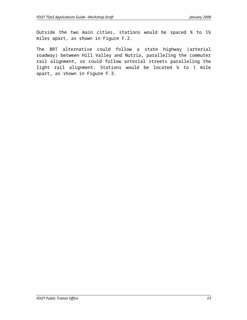
The light rail alternative would operate on city streets in Hill Valley before entering an abandoned railroad right-of-way that would take it all the way to the downtown Nutria transit center. Outside the two main cities, stations would be spaced ¾ to 1½ miles apart, as shown in Figure F.2.

The BRT alternative could follow a state highway (arterial roadway) between Hill Valley and Nutria, paralleling the commuter rail alignment, or could follow arterial streets paralleling the light rail alignment. Stations would be located ½ to 1 mile apart, as shown in Figure F.3.



Figure F.1Commuter Rail Alternative

Figure F.2Light Rail Alternative



Figure F.3BRT Alternatives

LOS MEASURES TO BE APPLIED

Transit-auto travel time

Passenger load

Service frequency

Service coverage

DATA NEEDS

Answering the transit agency’s questions will require the following data:

Future Travel Times. Horizon year (assumed to be 2030 in this example) peak-period travel time data will be required for automobiles, BRT, light rail, and commuter rail.

o Automobile travel time data will be available from the regional planning model.

o BRT travel times can be derived from the auto travel times produced by the regional planning model, using a procedure developed by FDOT described later. For a given route, an analyst would need to know the average bus stop spacing, and the number of miles that the route operates on divided arterials, undivided arterials, collectors, one-way streets, and ramps and freeways, respectively.

o LRT travel times can be derived from assumed speed limits for different track sections, typical LRT acceleration and deceleration characteristics, and assumed station dwell times.



o Commuter rail travel times can be estimated from information given in the TCQSM, given assumed station spacings and station dwell times.

Ridership demand for the corridors. Ridership in a corridor where local bus service is being considered to be upgraded to BRT can be estimated using procedures in TCRP Report 118: BRT Practitioners’ Guide. Ridership for new modes (i.e., LRT and commuter rail) could be estimated from overall travel demands from the regional model and an assumed mode split based on similar services in other areas.

Transit vehicle passenger capacities and loading standards. The local transit agency should have vehicle capacities and loading standards for its current fleet, and data from peer agencies can be used for vehicle types being considered for the future, but not currently used locally.

Route locations. These have been developed as part of each alternative being analyzed.

Population and employment estimates at the TAZ level. These data will be available from the regional transportation model.

ANALYSIS STEPS

1. Transit-Auto Travel Time

Overview

Calculating transit-auto travel time LOS involves the following steps:

1. Obtain year 2030 automobile travel times from the regional model for the following trips:

a. The most direct route from Hill Valley to Nutria (used as the auto travel time component of the transit-auto LOS calculation, this also happens to be the same routing as that used by the southern BRT route alternative); and

b. The route followed by the northern BRT alternative (used to estimate future BRT travel times for the northern route).

2. Deriving light rail and commuter rail travel times based on the assumed train and route characteristics.

3. Adjusting auto and transit in-vehicle travel times, to reflect access time (e.g., walk, wait, parking, etc.) for both ends of the trip.

4. Calculating the LOS for each alternative and evaluating the results.



Automobile Travel Times

Based on data from the regional model, the average auto travel time from Hill City to Nutria during the weekday a.m. peak period is approximately 30 minutes.

Bus Travel Times

FDOT’s Transit Speed and Delay Study methodology can be used to convert modeled auto travel times to transit travel times. Two options are available, depending on the level of detail desired. In the first option, transit travel times for each roadway link can be estimated directly within the model by multiplying the auto travel time for a link (i.e., the link distance divided by the link speed) by the appropriate factor for the link’s facility type. However, because these factors were developed using local bus routes and local bus stop spacing, they would produce speeds that would be lower than BRT route speeds. Instead, the second option, which incorporates both link travel time factors and number of stops made, is preferable.

For a corridor of interest, trace the route from beginning to end along the modeled roadway network. Sum the length traveled along each facility type (e.g., collector or divided arterial), and also sum the total auto travel time for each facility type. Working with the model data within GIS software can speed up this process. The results might look something like Table F.1 for a particular route.

Table F.1Example Modeled Auto Travel Time Data for the BRT Alternatives

Facility Type (FT) Total Distance (miles)

Auto Travel Time (sec)

Northern AlternativeFreeways and Ramps (FT 10, FT 70)

0.0 0

Divided Arterials (FT 20) 0.0 0Undivided Arterials (FT 30) 2.0 327Collectors (FT 40) 8.3 1,494One-way Streets (FT 60) 0.0 0

Southern AlternativeFreeways and Ramps (FT 10, FT 70)

0.0 0

Divided Arterials (FT 20) 0.0 0Undivided Arterials (FT 30) 9.1 1,489Collectors (FT 40) 0.4 72One-way Streets (FT 60) 0.8 240

Although most regional travel models define a variety of different facility types within a particular group (e.g., FT 21, 22, and 23 may all represent different types of divided arterials), this method treats all the sub-types the same (i.e., FT 21-23 are all treated as FT 20).



Next, count the number of BRT stations planned along each facility type, as shown in Table F.2.

Table F.2Number of Stations Along Each BRT Alternative

Facility Type (FT) Total Distance (miles)

# of Stops

Northern AlternativeFreeways and Ramps (FT 10, FT 70)

0.0 0

Divided Arterials (FT 20) 0.0 0Undivided Arterials (FT 30) 2.0 3Collectors (FT 40) 8.3 15One-way Streets (FT 60) 0.0 0

Southern AlternativeFreeways and Ramps (FT 10, FT 70)

0.0 0

Divided Arterials (FT 20) 0.0 0Undivided Arterials (FT 30) 9.1 15Collectors (FT 40) 0.4 1One-way Streets (FT 60) 0.8 2

From FDOT’s Transit Speed and Delay Study, the equation for estimating bus speeds from auto speeds and number of stops is: a1 * (Auto Time) + a2 * (Number of Stops). The values to use for the a1 and a2 factors are given in Table F.3.

Table F.3Transit Travel Time Factors: Calculations Outside FSUTMS

Facility Type (FT) a1 a2Freeways and Ramps (FT 10, FT 70)

1.000 30.0

Divided Arterials (FT 20) 1.196 32.5Undivided Arterials (FT 30) 1.222 20.7Collectors (FT 40) 1.180 21.9One-way Streets (FT 60) 1.299 24.2

Applying the factors in Table F.3 to the auto travel times and number of stops in Exhibits 4 and 5 produces the bus travel time estimates given in Table F.4. For example, for undivided arterials for the southern alternative (1.222 * 1489) + (20.7 * 15) = 2,130 seconds.

Table F.4Example Bus Travel Time Estimate Results

Bus Travel Time (sec)



Facility Type (FT) Northern Alternative

Southern Alternative

Freeways and Ramps (FT 10, FT 70)

0 0

Divided Arterials (FT 20) 0 0Undivided Arterials (FT 30) 462 2,130Collectors (FT 40) 2,091 107One-way Streets (FT 60) 0 360

Summing the results from Table F.4, dividing by 60 seconds per minute, and rounding, the in-vehicle portion of the transit trip would take about 43 minutes for either alternative.

Commuter Rail Travel Time

When station locations, track conditions, grades, and train characteristics are known, a train simulation model is the best tool for estimating train speeds and travel times. In the absence of that information, Exhibit 5-75 from the TCQSM (reproduced below as Table F.5) can provide a first-cut, planning-level estimate of commuter rail speeds.

Table F.5Commuter Rail Operating Speeds

Average Operating Speed (mph)Station Spacing

(miles)P/W = 3.0 P/W = 5.8 P/W = 9.1

Average Dwell Time = 30 seconds1.0 16.8 20.3 22.32.0 25.8 30.9 35.04.0 36.4 44.1 48.65.0 40.3 48.7 52.7

Average Dwell Time = 60 seconds1.0 14.8 17.4 18.82.0 23.3 27.4 30.64.0 33.8 40.4 44.15.0 37.8 45.0 48.5

SOURCE: TCRP Report 100, Transit Capacity & Quality of Service Manual, 2nd Edition, Exhibit 5-75P/W = locomotive power-to-weight ratioAssumes an 80-mph speed limit, no grades, and no delays due to other trains

Based on guidance given in the TCQSM, a power-to-weight ratio of 5.8 is typical for a locomotive-hauled commuter rail train, and an average dwell time of 60 seconds is the more appropriate assumption for peak periods. The average operating speed can be interpolated from the table for station spacings different than those given in the table (e.g., 3 miles in this example).



Although the table was designed for 80-mph speed limits (i.e., FRA track class 4), it is also applicable to lower speed limits (e.g., 60 mph, track class 3) for shorter station spacings and lower power-to-weight ratios, as trains never reach the top speed before having to begin slowing for the next station. For this example, it is assumed that the mainline section of the route will have a passenger train speed limit of at least 60 mph. The mainline portion of the route is 9.4 miles long. The 0.4-mile portion of track departing the Hill Valley station is a branch line with a 30-mph speed limit, while the 0.3-mile portion of track in Nutria would be constructed in a street median and would have a 20-mph speed limit (the same as the adjacent roadway).

Given this information, if the entire line operated at the higher speed limit, the average speed would be 33.9 mph (interpolating between 27.4 and 40.4 in Table F.5). It would take a train about 1,070 seconds to travel from Hill Valley to Nutria under these circumstances. Delays caused by the short, slower track sections at either end of the route would add about 21 seconds to this time, resulting in an overall in-vehicle travel time of about 18 minutes.

Light Rail Travel Time

The proposed light rail line would operate at a top speed of 25 mph along the 0.8-mile, on-street portion section of the line in Hill Valley, and at a top speed of 55 mph along the remaining 10.2 miles of the route. The TCQSM does not provide a look-up table of average light rail speeds for different combinations of speed limits, station spacings, and dwell times; however, it does give typical LRT acceleration and deceleration values (4.3 ft/s2), which can be used to derive an average speed.

A speed of 55 mph is equivalent to 81 feet per second. The distance traveled during acceleration to this speed (or deceleration from this speed) is ½at2, where a is the acceleration rate and t is the time required to accelerate to top speed (81 ft/s divided by 4.3 ft/s2 equals 18.8 s). Thus, it takes a train about 760 feet to accelerate out of a station and 760 feet to decelerate into a station, with the remaining distance between stations operated at top speed. Since no stations in the higher-speed track section are less than (760 * 2 = 1,520 feet) apart, a train will always reach its top speed.

There are 11 stations in the 55-mph track section, which is 10.2 miles long. Therefore, the average station spacing is about 4,900 feet. Of this distance, (4,900 – 1,520 = 3,380 feet) would be operated at top speed, and would take about (3,380 / 81 = 41.7 seconds) to cover. Thus, the average travel time between stations would be: 18.8 seconds acceleration + 41.7 seconds cruise + 18.8 seconds deceleration, or about 79.3 seconds total. Therefore, the total travel time between stations (excluding dwell) would be (11 * 79.3 = 872 seconds). Repeating the same process for the 25-mph section, the travel time for that section (excluding dwell) would be about 140 seconds. If the average dwell time at each of the 13 intermediate stations is 30 seconds, the total dwell time would be 390 seconds. Thus, the total in-vehicle travel time from Hill Valley to Nutria would be (872 + 140 + 390 = 1,402 seconds) or about 23 minutes.



Travel Time Adjustments

Transit-auto travel time LOS is based on door-to-door travel times. Therefore, the modeled in-vehicle times must be adjusted for such things as parking and walking time (for autos), and walking and waiting time (for buses and trains). For this example, 5 minutes was added to the auto travel times to account for time to park and walk to one’s destination (this adjustment could also have been made on a location-by-location basis). Similarly, 11 minutes was added globally to commuter rail, light rail, and BRT travel times for walk access to the boarding stop (3 minutes), wait time at the stop (5 minutes), and walk access from the alighting stop (3 minutes), based on recommendations given in the TCQSM. Thus, the door-to-door travel time is 35 minutes for auto, 54 minutes for either BRT alternative, 34 minutes for light rail, and 29 minutes for commuter rail.

LOS Calculation

Transit-auto travel time LOS is calculated by subtracting auto travel times from transit travel times. Table F.6 provides the table from the TCQSM used to convert the travel time differences to a level of service grade.

Table F.6Transit-Auto Travel Time LOS Thresholds

LOSTravel Time

Difference (min) CommentsA ≤0 Faster by transit than by automobileB 1-15 About as fast by transit as by automobileC 16-30 Tolerable for choice ridersD 31-45 Round-trip at least an hour longer by transitE 46-60 Tedious for all riders; may be best possible in

small citiesF >60 Unacceptable to most riders

SOURCE: TCRP Report 100, Transit Capacity & Quality of Service Manual, 2nd Edition, Exhibit 3-30

The travel time differences by alternative are -6 minutes for commuter rail (LOS A), -1 minute for light rail (LOS A), and +19 minutes for either BRT alternative (LOS C).

Applying the Results

Either rail alternative in this example would provide a faster door-to-door trip than the automobile, suggesting that either type of service would be very attractive to choice riders. The LOS C result for BRT, while not bad, does indicate that BRT service would be less attractive to riders than LRT or commuter rail in this particular area of comparison. (Although a comparison with the existing local bus service was not performed in this example, it would likely be at least one LOS grade worse, indicating that BRT would provide more attractive travel times than the existing bus service.) The BRT



alternatives could also be refined at this point to identify whether transit priority treatments could result in faster, more competitive travel times.

2. Service Frequency

Overview

This portion of the application demonstrates the use of LOS measures as planning and design inputs, as opposed to evaluation tools. Given a forecasted peak-period demand for transit service, how many buses per hour would be needed to meet that demand, while avoiding pass-ups?

This process involves the following steps:

1. Forecasting ridership.

2. Identifying typical vehicle seating capacities, typical passenger arrival characteristics, and typical loading standards.

3. Converting an hourly passenger demand into a peak-15-minute or peak-vehicle passenger demand.

4. Calculating the number of buses or trains needed in the peak hour to avoid overcrowding.

Forecasting Ridership

Techniques for forecasting ridership are outside the scope of these guidelines. Refer to the earlier “Data Needs” section for suggestions on how to forecast ridership. For the sake of example, it is assumed that BRT and LRT would operate at minimum 10-minute policy headways, while commuter rail would operate at 30-minute headways, due to the need to accommodate freight trains. Further, it is assumed that the applicable ridership forecasting methods produce year 2030 peak-load-point, peak hour ridership estimates of 370 riders for both BRT alternatives and commuter rail, and 530 riders for light rail.

Vehicle and Passenger Characteristics

For the sake of this example, it is assumed that BRT would be operated using 60-seat articulated buses, LRT would be operated using two-car trains with 72 seats per car, and commuter rail would be operated with two-car diesel multiple-unit (DMU) trains with 74 seats per car. Typical practice is to design for some standees on BRT and LRT, but not on commuter rail. As shown in Table F.7, the corresponding passenger loading LOS for commuter rail would LOS C, while it would be LOS D for BRT and LRT.

Table F.7Passenger Loading LOS Thresholds

LO Passengers Standing Comments



S per Seat

Area per Passenger

(sq. ft.)A 0.00-0.50 No passenger need sit next to anotherB 0.51-0.75 Passengers can choose where to sitC 0.76-1.00 All passengers can sitD 1.01-1.25* ≥3.9 Comfortable standee load for urban

transitE 1.26-1.50* 2.2-3.8 Maximum schedule load for urban

transitF >1.50* <2.2 Crush load

SOURCE: Adapted from TCRP Report 100, Transit Capacity & Quality of Service Manual, 2nd Edition, Exhibit 3-26*Approximate values for comparison

The TCQSM also provides guidance on how passenger arrivals are spread throughout an hour, for different transit modes. One can imagine that the number of passengers wanting to ride on a bus or train will vary over the course of an hour: some transit vehicles will be more heavily loaded than others. To be reasonably sure that the most heavily loaded vehicles during the hour will not exceed the loading standard, a peak hour factor should be applied. This factor creates the equivalent hourly demand that would result if peak-15-minute demands were sustained over the entire hour. Recommended peak hour factors given by the TCQSM, in the absence of local information, are 0.75 for buses scheduled at regular headways, 0.75 for light rail, and 0.90 for commuter rail.

Over the entire peak hour, the average load on a BRT bus at the route’s peak load point would be (370 passengers / 6 buses per hour = 62 passengers per bus). This is equivalent to a load factor of 1.03 (62 passengers / 60 seats), corresponding to LOS D. However, the most heavily loaded buses would have an average load of (370 riders/ 6 buses per hour / 0.75 peak hour factor = 82 passengers) at the peak load point, corresponding to a load factor of 1.37, which would likely be in the LOS E range, according to Table F.7, and which would exceed the desired loading standard. If service were increased to 8 buses per hour, the average load during the peak 15 minutes would be 62 passengers, or LOS D, thus meeting the standard. A higher frequency would likely attract more passengers, so another iteration of the ridership forecasts might be warranted.

For light rail, the peak-15-minute load at the maximum load point would be (530 passengers / (6 trains per hour * 2 cars per train) / 0.75 = 59 passengers per car), a load factor of 0.82, or LOS C. If service was operated at 12-minute headways, the load factor would be 0.99 (still LOS C), while if service was operated at 15-minute headways, the load factor would be 1.23 (likely at the high end of LOS D, depending on the amount of standing area provided within the LRT cars).

Finally, for commuter rail, the more heavily loaded of the two trains would have (370 passengers / (2 trains per hour * 2 cars per train) / 0.90 = 103 passengers per car), well above a car’s seating capacity of 74. Since no more



than two trains per hour could be operated due to the need to accommodate freight trains, more cars would need to be added to each train to provide enough seating capacity. A three-car train would result in an average of 69 passengers on board the more heavily loaded train, corresponding to a load factor of 0.93 and meeting the desired LOS C standard.

Service Frequency

This check of passenger loads helped identify the minimum service frequency needed to produce the desired loading standard for each mode, thus maximizing each alternative’s efficiency. A total of 8 buses per hour would be required for BRT, 4 two-car trains per hour for LRT, and 2 three-car trains per hour for commuter rail. As shown in Table F.8, these frequencies correspond to LOS A, LOS C, and LOS D, respectively.

Table F.8Service Frequency LOS Thresholds

LOS

Average Headway

(min)

Frequency (buses/hour)

CommentsA <10 >6 Passengers do not need schedulesB 10-14 5-6 Frequent service, passengers consult

schedulesC 15-20 3-4 Maximum desirable time to wait if bus

missedD 21-30 2 Service unattractive to choice ridersE 31-60 1 Service available during the hourF >60 <1 Service unattractive to all riders

SOURCE: TCRP Report 100, Transit Capacity & Quality of Service Manual, 2nd Edition, Exhibit 3-12


Passenger loading LOS was used as a design standard, from which required service frequencies and train and bus sizes were determined. From a frequency perspective, the BRT alternatives would be more attractive to passengers than the rail alternatives, while from a comfort perspective, the commuter rail alternative would be slightly more attractive than the other alternatives.

3. Service Coverage

Overview

Service coverage LOS measures how much of a defined area that is likely to generate sufficient ridership to support fixed-route transit service is actually served. Because it is an area-wide measure, service coverage LOS is not directly applicable to a corridor evaluation, such as that being conducted in this application. However, a portion of the process used to measure service coverage LOS can also be used to determine the number of people and jobs



that would be directly served by a particular premium transit service. The following steps are involved:

1. Obtaining existing and/or future household and employment totals for each of the regional model’s traffic analysis zones (TAZs).

2. Using GIS software, buffer each BRT or rail station in the corridor, to determine the area served by premium transit. This step can optionally include adjustments to the service area to reflect street connectivity and other factors in the station vicinities.

3. Determine the number of people and jobs located within these buffer areas.

Household and Employment Totals

Household and job totals by TAZ can be obtained from the regional planning model, and each TAZ’s area can be calculated using GIS software. Figure F.4 shows the locations of the TAZs within the study area (outlined in purple. For the purposes of this exercise, year 2020 household and job forecasts are being used.

Figure F.4TAZ Locations Within the Premium Transit Corridor

Identifying Transit-Served Areas

The TCQSM considers areas located within ½ mile of a BRT or rail station to be served by transit. Using GIS software, stops and stations can be buffered by these distances, and the buffers subsequently merged together, to identify the area served by transit. (The TCQSM provides optional methods to reduce these distances to reflect lack of street connectivity, street crossing difficulty, grades, and presence of a large population of elderly people.) Figures F.5-F.7 show the areas that would be served by the proposed commuter rail, light rail, and BRT stations, respectively.

Using GIS software, union the transit service buffer with the TAZ layer, creating a cookie-cutter effect on the TAZ layer, with the TAZs being subdivided into smaller areas that are entirely served, or entirely not served



by transit. Calculate the areas of these sub-TAZs and store the result in a new field (i.e., do not overwrite the field containing the parent TAZ’s area).

Figure F.5Commuter Rail Station Buffer Areas

Figure F.6Light Rail Station Buffer Areas



Figure F.7BRT Station Buffer Areas

One method suggested by the TCQSM for allocating persons and households to sub-TAZs is to assign it in proportion to each sub-TAZ’s share of the parent TAZ’s area. That is, if the parent TAZ is 10 acres in size and contains 150 jobs, and of its sub-TAZs is 6 acres in size, then 60% of the parent TAZ’s jobs, or 90 jobs, would be assigned to the sub-TAZ. If desired, the allocation can be refined further by only allocating jobs to portions of the TAZs zoned for employment uses, for instance, or by allocating households to portions of the TAZs zoned for residential uses, in proportion to the allowed residential densities within different portions of the TAZ. For existing conditions analyses, an additional refinement would be to only assign population or jobs to portions of the TAZ that have actually been developed.

Calculating Population and Jobs Served

Once households (or population) have been assigned to the sub-TAZs, the final step is to simply sum up the total population and jobs within walking distance of each station. If the regional model provides household totals, these can be converted to population based on average household size data for the area, available from the Census Bureau. Table F.9 shows the results for the four premium transit alternatives.

Table F.9Population and Jobs Within Walking Distance of Premium Transit

Stations

Alternative Population

Jobs

Commuter Rail 17,900 22,700

Light Rail 53,200 75,400

BRT (northern alignment)

74,700 95,000



BRT (southern alignment)

76,300 87,100


As would be expected, the more frequent the station spacing, the greater the total population and jobs within walking distance. Comparing the two BRT alignments, which have similar station spacings, the southern alignment serves a greater residential population, but fewer jobs. If desired, similar types of evaluations could be done that also consider the population within walking distance of feeder bus service that would connect to the proposed premium transit service and/or the population living within the market area of park-and-ride lots serving the premium transit lines.

PUTTING IT TOGETHER

This application has demonstrated how the transit LOS measures and procedures can be used to develop quantifiable measures that can be used to compare premium transit alternatives to each other. These are not the only measures that should be included in the analysis—for example, relative capital and operating costs, potential ridership, and consistency with local transportation goals and policies should also be considered—but they do help evaluate how well the service would work from a customer point-of-view.

As shown in Table F.10, the rail alternatives would be attractive to passengers from a travel-time standpoint, while the BRT alternatives would be attractive from a service frequency standpoint. All of the alternatives would have well-utilized vehicles during peak hours, as indicated by the passenger load LOS results. Commuter rail’s passengers would be more likely to arrive by feeder bus or private auto, while substantial potential markets are located within walking distance of either of the BRT alternatives. Although light rail makes fewer stops than BRT, the total population and jobs located within walking distance of LRT stations would still be quite high.

Table F.10 Results Summary

Level of Service

Alternative

Transit-Auto

Travel Time

Passenger Load

Service Frequency

Population

Served

Jobs Served

BRT (North) C D A 74,700 95,000BRT (South) C D A 76,300 87,100Light Rail A D C 53,200 75,400Commuter Rail

A C D 17,900 22,700


application #5: premium transit alternatives analysis transit alternatives.doc · web viewtable f.4...

Documents