O.1

APPENDIX O (SELECTED QUESTIONS FROM OLD EXAMS) Midterm 1 M1.I Short questions (14 points each) 1. (CHAPTER LN III). Bank A gives the following quotes: BOB/USD=8.0000-25. The Euro one-year interest rates for the BOB, iBOB, and for the USD, iUSD, are 10(1/4)-(3/4) and 8(1/8)-(1/4). A. What is a possible quotation for the 180-day year BOB/USD forward exchange rate? (BOB= Bolivian peso.) B. Chivas Bank quotes FCB

t,180=8.132-8.15 BOB/USD. Is arbitrage possible? If so, design a covered arbitrage strategy to take advantage of Chivas Bank’s quote. ANSWER: (A.) Determination of bounds: we need to calculate the bounds for the forward rate, Ubid and L ask. Ubid = Sask,t[(1+iask,dxT/360)/(1+ibid,fxT/360)] = 8.0025 BOB/USD [1.05375/1.040625] = 8.1034 BOB/USD. Lask = Sbid,t[(1+ibid,dxT/360)/(1+iask,fxT/360)] = 8.0000 BOB/USD [1.05125/1.04125] = 8.07683 BOB/USD. Fask,t,T

Fbid,t,T Lask=8.07683 Ubid=8.1034 Ft,T (BOB/USD) Possible quote: Ft,180=8.0910-8.0975 BOB/USD. (B) FCB

t,180=8.132-8.15 BOB/USD violates the Ubid bound => Arbitrage is possible. Covered arbitrage strategy: 1. Borrow BOB 1 at iask,BOB=10.75% for 180 days. 2. Convert BOB 1 to USD at St,bid=8.0025 BOB/USD 3. Deposit USD 0.12496 at ibid,USD=8.25% for 180 days. 4. Sell the USD forward at FTB

t-180,bid = 8.132 BOB/USD.

O.2

2. (CHAPTER LN II). Mexico has a floating exchange rate system. The Mexican peso (MXP) is appreciating against the USD. The Central Bank of Mexico decides to intervene to stop the appreciation of the MXP. The Central Bank of Mexico does not want to affect local interest rates. With the help of a graph, describe what the Central Bank authorities can do. ANSWER: Original Situation: Point A (S0= 9 USD/MXP and i0=10%) CB intervention in FX market (buy USD-sell MXP): Point B (S1= 10 USD/MXP and i0=9%) Sterilization intervention (OMO:buy MXP-sell Letes) Point C (S1= 10 USD/MXP and i0=10%) FX Market St FX intervention S0

(MXP/USD)

B S1= 10 A S0= 9 D1

D0 Quantity of USD Money Market MS,0 i

OMO

A=C MS,1 i1= 10 B i0= 9

FX L0 intervention Quantity of Money (MXP) The Central Bank of Mexico uses an OMO to stop the appreciation of the MXP against the USD. The OMO consists of selling Letes (Mexican Short-term Treasury bonds) and receiving MXP, thereby, reducing domestic credit (money supply goes back to MS,0). The OMO brings the Money Market back to A(=C), where the interest rate is i0.

O.3

3. (CHAPTER LN I). Kramerica Bank gives the following quotes: St = .6102-.6110 USD/CHF, and St= 1.6170-1.6190 USD/GBP. In addition, Kramerica Bank quotes Sbid= 2.6575 CHF/GBP. Is arbitrage possible? If so, design a triangular strategy to take advantage of Kramerica’s quotes. ANSWER: (i) Calculate the CHF/GBP cross-rates. Sbid,CHF/GBP = Sbid,CHF/USDxSbid,USD/GBP=[(1/.6110) CHF/USD]x[(1.6170) USD/GBP]= 2.6465 CHF/GBP. Sask,CHF/GBP=Sask,CHF/USDxSask,USD/GBP = [(1/.6102) CHF/USD]x[(1.6190) USD/GBP] = 2.6532 CHF/GBP. (ii) Kramerica’s bid quote for the CHF/GBP is too high (overvaluation of the GBP against the CHF). (1) Borrow CHF 1; (2) exchange it for USD .6102; (3) exchange the USD .6102 for GBP .3769; (4) sell GBP and buy CHF using Sbid=2.6575 CHF/GBP. => we get CHF 2.6575 x .3769 = CHF 1.00162. 4. (CHAPTER LN III). Suppose you are given the following data: St = 110 JPY/USD iJPY,1-yr = 2% iUSD,1-yr = 6% Ft,1-yr = 108 JPY/USD. (A) Is arbitrage possible? (Hint: Calculate the IRPT forward rate). (B) If IRPT does not hold, design a covered arbitrage strategy. Calculate the arbitrageur’s profits. (C) Briefly discuss, the capital flows observed in Japan if the above prices persist. ANSWER: (A) Ft,1-yr = St (1 + id) /(1 + if) = 110 JPY/USD x (1 + .02)/(1 + .06) = 105.84 JPY/USD (108 JPY/USD) YES, arbitrage is possible. (B) The forward USD is overvalued (Ft,1-yr = 108 > FIRPT

t,1-yr =105.84). Therefore, a covered arbitrage strategy should involve selling the USD forward. Steps: (1) Borrow JPY 1 at 2% for 1 year. (2) Convert to USD at 110 JPY/USD. (3) Deposit in USD at 6% for 1 year (4) Sell USD forward at 108 JPY/USD. In one year, we’ll observe the following cash flows. We’ll receive (in JPY) = (USD 1/110) x 1.06 x 108 JPY/USD = JPY 1.0407 We’ll pay (in JPY) = JPY 1 x 1.02 = JPY 1.02 Profits = JPY 1.0407 – JPY 1.02 = JPY .0207 (2.07%) (C) Japan observes: p = (108 - 110)/110 = -.01818 and iJPY - iUSD = .02 - .06 = -.04. Since p > iJPY - iUSD, capital flies from Japan to the U.S. For example, Japanese investors will sell Japanese government bonds. The proceeds of these sales will be invested in U.S. assets ( not an equilibrium situation).

O.4

5.- (CHAPTERS LN I-VIII).You are a Swiss Investor and only care about Swiss Franc returns. You follow a multi-country CAPM approach. Design an investment for the following scenarios (you want to invest in the markets mentioned): a.- you're bullish on the Japanese yen (JPY), but unsure of the Japanese economy. b.- you're bullish on the Madrid Stock Exchange, but unsure about the peseta (the Spanish currency). c.- you're bullish on the computer industry and on the DEM, but you forecast a bear market in Germany. d.- you forecast a bigger than usual trade deficit in the U.S. and a strong U.S. stock market. e.- you forecast interest rates in Bolivia are going to decrease, but the Bolivian economy is in a recession. ANSWER: a) Low JPYs stocks b) High Spanish stocks (and hedge FX exposure) c) Low computer industry (no hedge FX exposure) d) Exchange rate USD/CHF . Then, hedge USD exposure. High stocks in the US e) Exchange rate BOB/CHF . It might jump start the stagnant Bolivian economy: Buy high Bolivian stocks, but hedge FX exposure 6. (CHAPTER LN VII). Mr. Splinter, a U.S. delta hedger, wants to hedge CHF 10 million for a year. He decides to buy put options with a strike price of 80 at a premium of 2.55 cents per CHF. The delta, , of this contract is (-1.2), with a gamma of 0.15. The spot rate is USD .7890 per CHF. Suppose that the PHLX option contract covers CHF 62,500 (a contract includes 62,500 CHF puts). a) Determine the number of number of contracts Mr. Splinter should buy. b) Two months later the spot rate was .7990 USD/CHF. What is the delta at this spot rate? How many contracts should Mr. Splinter buy/sell to maintain a perfect hedge? ANSWER: (a) CHF 10,000,000 to hedge. N = number of contracts = -10,000,000/[-1.2 x 62,500] = 133.33 133 contracts (b) new = + 1 x = -1.20 + .15 = -1.05 Nnew = -10,000,000/[-1.05 x 62,500] = 152.38 152 contracts. Mr. Splinter needs to buy 19 contracts, to add to his 133 contracts.

O.5

7. (CHAPTER LN III). It is March 1999. You read in the Economists that a Big Mac in London sells for GBP 1.90, while in New York it sells for USD 2.43. The exchange rate is 1.61 USD/GBP. (A) According to purchasing power parity (PPP), what should be the USD/GBP exchange rate? (B) If you believe in PPP, what kind of signal (buy, hold, sell) have you generated? (C) Based on the real exchange rate, which country is more competitive? Briefly, discuss the implications of your findings. ANSWER: (A) SPPP

t = USD 2.43/GBP 1.90 = 1.28 USD/GBP. (B) According to PPP, the GBP is overvalued (25.88%). Therefore, PPP has generated a sell GBP signal. (C) Rt = St Pf / Pd = [1.61 USD/GBP x GBP 1.90]/[USD 2.43] = 1.2588 ( Rt is different from one!). The U.K. is less competitive than the U.S. since its (Big Mac) prices are higher than U.S. prices, after taking into account the nominal exchange rate. Over time, we expect the GBP to depreciate against the USD. 8. (CHAPTER LN V). You work for Valdano Co. Valdano Co. is a U.S. hedge fund that has a long position in Swiss bonds, valued at USD 50,000,000. They use a GARCH(1,1) model to forecast the monthly volatility of the USD/CHF exchange rate. Valdano Co. uses monthly observations, measured in percentage changes, to estimate the GARCH model. Valdano Co. obtains the following estimates for the variance parameters: 0 = .003, 1 = .150, and ß1 = .930. The estimate for this month’s (August) conditional variance is 2

AUG = 0.002. At the end of August, the exchange rate is SAUG = .7050 USD/CHF, while Valdano had a forecast SF

AUG = .6900 USD/CHF. The exchange rate in July was SJUL = .6850 USD/CHF (A) Valdano Co. asks you to forecast the variance next month (September). ANSWER: sF

AUG = (.6900 - .6850)/.6850 = 0.0073 sAUG = (.7050 - .6850)/.6850 = 0.0292 SEP = (sAUG - sF

AUG) = 0.0292 – 0.0073 = 0.0219 2

SEP = 0.003 + 0.150 (0.0219)2 + 0.930 (0.002) = 0.004932 That is, the volatility forecast for September is SEP = 7.023%. (B) Now, Valdano wants to calculate the September’s VAR of its exposure to changes in the USD/CHF exchange rate. Valdano uses a 95% confidence interval for VAR calculations. Briefly explain VAR estimate. ANSWER: VAR (mean) = W0t. = USD 50M x 1.65 x 0.07023 x 1 = USD 5,793,975.00 That is, the maximum one-month loss of this portfolio is USD 5.794M => In this 95% C.I., the worst case scenario for Valdano’s Swiss bond position: USD 50M – USD 5.794M = USD 44.206M. Note: , the volatility, is monthly. Given that the estimated VAR (mean) is also monthly (September), t=1.

O.6

9. (CHAPTER LN VIII). Chambers Corporation will receive DEM 1,000,000 in 180 days. It considers using (1) a forward hedge, (2) an option hedge, or (3) no hedge. Its analysts develop the following information, which can be used to assess the alternative solutions: • Spot rate of mark as of today = .65 USD/DEM • 180-day forward rate of mark as of today = .67 USD/DEM • Interest rates are as follows: 180-day deposit rate: 5.5% in Germany, and 6.0% in the U.S. 180-day borrowing rate: 6.0% in Germany, and 7.0% in the U.S. • A DEM call option: expires in 180 days, exercise price of .68 USD/DEM, and a premium of USD .02. • A DEM put option: expires in 180 days, exercise price of .70 USD/DEM, and a premium of USD .03. • Chambers Corporation forecasted the future spot rate in 180 days as follows: Possible Outcomes Probability .63 USD/DEM 20% .66 USD/DEM 60% .74 USD/DEM 20% Which strategy would you recommend to Chambers Corporation? Why? ANSWER: (1) Forward Hedge: Sell DEM 180 days forward. USD to be received in 180 days = DEM 1,000,000 x .67 USD/DEM = USD 670,000. (2) Option Hedge: Purchase put options. Exercise price = .70 USD/DEM; premium = USD .03

Possible St+180 Premium per Unit for Option

Exercise? (X=USD .70)

Total USD Receivedper Unit

Total USD Amount (DEM 1,00,000)

Probability

USD .63 USD .03 YES USD .66910 USD 669,100 20%

USD .66 USD .03 YES USD .66910 USD 669,100 60%

USD .74 USD .03 NO USD .70910 USD 709,100 20%

E[USD to be received in 180 days] = USD 677,100 (3) Remain Unhedged: Purchase CHF 100,000 in the spot market 180 days from now.

Future Spot Rate in 180 Days Total Amount (USD 1,000,000) Probability

USD .63 USD 630,000 20%

USD .66 USD 660,000 60%

USD .74 USD 740,000 20%

E[USD to be received in 180 days] = USD 670,000 Recommendation: Use put options, but a risk-lover might consider the no-hedge strategy.

O.7

10. (CHAPTER LN VIII). Mr. Pitman is the owner of a small publishing company in New York that specializes in distributing books to Europe. Mr. Pitman monthly revenue is EUR 250,000 a month. Mr. Pitman wants to set up a USD/EUR naive hedge that would ensure his ability to make affordable purchases in the U.S., should the EUR collapse. In particular, he is very worried about a potential depreciation of the EUR against the USD in December. Mr. Pitman wants flexibility, so he decides to use American option contracts. Mr. Pitman’s broker charges a flat fee of USD 15 and the exchange charges USD 1.50 per contract. A. Specify what type of options should Mr. Pitman use (calls or puts). B. How many standardized PHLX contracts should Mr. Pittman buy? C. Using the information given in the WSJ clip, construct: i) at the money/in-the-money December hedge. ii) out-of-the money December hedge. iii) a collar. (Specify strike prices and costs.) Briefly discuss the advantages and disadvantages of each strategy. Which one would you recommend to Mr. Pitman? (Why?) ANSWER: (A) Mr. Pitman should use puts (right to sell EUR) (B) Number of contracts = EUR 250,000/[62,500/contract] = 4 contracts. (C) At-the-money (X=1.06 USD/EUR, premium=USD .0283) Cost: a. premium USD .0283 per EUR USD 7,075 (=USD 0.0283 x 250,000) b. broker fee USD 15 + USD 1.50 per contract USD 21 Advantage: sets a floor close to today’s St (1.0554 USD/EUR). The floor is set at USD 265,000. Disadvantage: cost = USD 7,096. Out-of-the-money (X=1.04 USD/EUR, premium=USD .0170) Cost: a. premium USD .0283 per EUR USD 4,250 (=USD .0170 x 250,000) b. broker fee USD 15 + USD 1.50 per contract USD 21 Advantage: cost = USD 4271 (a cheaper alternative than the in-the-money/at-the money option) Disadvantage: sets a lower floor = USD 260,000

O.8

Collar: buy one put (X=1.04 USD/EUR, premium=USD .0170) and sell one call (X=108 USD/EUR, premium=USD 0.0056)

Cost: a. premium USD .0283 per EUR (paid) USD 4,250 a. premium USD .0056 per EUR (received) (USD 1,400) b. broker fee USD 15 + USD 1.50 per contract USD 42 Advantage: cost = USD 2,892 (the cheapest!) Disadvantage: sets a lower floor = USD 260,000 and also sets a cap = USD 270,000. Recommendation: The collar looks attractive, from a price perspective. It’s a cheap insurance alternative. Information from the WSJ PHILADELPHIA OPTIONS Friday, September 10, 1999 Calls Puts Vol. Last Vol. Last Euro 105.54 62,500 Euro-cents per unit. 102 Oct ... 0.01 3 0.38 102 Dec ... 0.01 5 0.49 104 Sep 3 0.74 90 0.15 104 Oct 7 1.70 ... ... 104 Dec 3 2.19 25 1.70 106 Dec 8 1.85 12 2.83 108 Oct 75 0.43 ... 0.01 108 Dec 17 0.56 3 3.68 112 Dec 2 0.08 1 7.81 Australian Dollar 65.37 50,000 Australian Dollars-cents per unit. 64 Oct ... 0.01 20 0.31 65 Sep 20 0.30 ... ... 66 Oct 30 0.42 ... 0.01 British Pound 163.52 31,250 British Pounds-European Style. 161 Sep 32 0.82 ... ... 162 Oct 32 1.54 ... 0.01 31,250 British Pounds-cents per unit. 159 Oct ... ... 4 0.63 161 Sep 4 0.94 ... 0.01

O.9

11. (CHAPTER LN VIII). It is March 3, 2011. Malone, a U.S. company, exports baseball equipment to Taiwan. Malone expects to receive a payment of TWD 50 million in August 1, 2011 (TWD=Taiwanese Dollar). Malone decides to hedge this exposure using an August forward contract, which expires on August 1, 2011. The 3-month, 4-month and 5-month Taiwanese interest rates are 3.5%, 3.7% and 4%, while the 3-month, 4-month and 5-month U.S. interest rates are 1%, 1.1% and 1.3%, respectively. On March 3, the spot exchange rate is 29.78 TWD/USD and the August 1 forward trades at 30.12 TWD/USD. (A) Use the information given in the attached Excel output (based on 10 years of monthly changes) to calculate: i) The VAR associated with Malone’s open position (use a 97.5% C.I.). ii) The worst case scenario for Malone. (B) Calculate the amount to be received on August 1, using a forward hedge. (C) Calculate the amount to be received on August 1, using a money market hedge. (D) Assume the payment is made on July 11, 2011. On July 11, the spot exchange rate is 30.51 TWD/USD, the Taiwanese short-term interest rate is 3.85% and the U.S. short-term interest rate is 1.5%. Calculate the value of the August 1 forward contract on July 11, 2011. (Use IRP to calculate the forward rate.) (E) (Continuation of question D) Calculate the hedger’s profits (losses). (F) Was the August 1 forward a perfect hedge? List all the factors that make the hedge imperfect. ● DATA The information below is based on monthly percentage changes from 2001:1 to 2010:12.

1-mo % change TWD/USD Mean -0.077% Standard Error 0.1329% Median -0.029% Mode ..... Standard Deviation 1.4495% Sample Variance 2.1 Kurtosis 0.561619 Skewness -0.26282 Range 8.2225 Minimum -4.365% Maximum 3.8576% Sum -9.202 Count 119

ANSWER: Note: Data is in terms of TWD/USD, but question is in terms of USD –i.e, USD=DC! UP = TWD 50 M (long) A. Transaction Exposure (TE): TWD 50 M x (1/29.78 TWD/USD) = USD 1.67898 M

O.10

Note: The monthly mean (TWD/USD) is -.0077 => The monthly mean (USD/TWD) is .0075 T= 5-mo 5-mo mean = .0077*5 = .0385 (3.85%) 5-mo SD = .014495*sqrt(5) = .0324 (3.24%) (i) VaR(97.5%) = USD 1.67898 M*[1+(.0385-1.96x.0324)] = USD 1.637 M (ii) The method used to approximate 5-mo mean returns cannot be used for extremes. Given the information, we need to make assumptions. Let’s assume the worst case 1-mo scenario (-.038576) also applies in 5-mo. Then, Worst case scenario = USD 1.67898 M*(1-.038576) = USD 1.614 M B. Amount to be received = TWD 50M x 1/(30.12 TWD/USD) = USD 1.66003 M C. Check lectures notes. But, note that MMH is a replication of IRP. Then, Ft,150=1/(29.78 TWD/USD) x (1+.013x5/12)/(1+.04x5/12)=.03321 USD/TWD => Amount to be received = TWD 50M x .3321 USD/TWD = USD 1.6605 M D. F July 11,,Aug 1 = 30.51 TWD/USD x (1+.0385x20/360)/(1+.015x20/360) = 30.549 TWD/USD DW was short THD at the (1/30.12) USD/THD forward rate (or long the USD at 30.12 THD/USD). Now, to close the HP we go long the THD at (1/30.549) USD/THD (or short the USD at 30.549 THD/USD). Value of forward contract = FMarch 3,,Aug 1 – FJuly 11,,Aug 1 = (1/30.12 – 1/30.549) = USD 0.00046584728 [1 + iUSD x (T/360)] [1 + .015x(20/360)] E. Total value of Forward position (HP) = 50M*USD 0.00046584728 = USD 0.023292364 => Total Amount to be received = TWD 50M x (1/30.51 TWD/USD) + USD 0.0233M = USD 1.6621069 M F. No! Basis changed from (30.12-29.78) = 0.34 to (30.549-30.51) = 0.039

O.11

12. (CHAPTER LN VIII). Mr. Boyd is the owner of a chain of pubs in Boston that sells Australian beers. Mr. Boyd’s monthly purchases of Australian beer are AUD 200,000 a month. Mr. Boyd wants to set up a USD/AUD naive hedge that would ensure his ability to make affordable purchases in Australia, should the AUD appreciate. In particular, he is very worried about a potential appreciation of the AUD against the USD in April. Today, the exchange rate is St = 0.9745 USD/AUD. Mr. Boyd wants flexibility, so he decides to use American option contracts. A. Specify what type of options should Mr. Boyd use (calls or puts). B. How many standardized PHLX contracts should Mr. Boyd buy? C. What is April’s transaction exposure for Mr. Boyd? D. Using the information given in the WSJ clip (see next page), construct: i) at the money/in-the-money April hedge (choose closest in-the-money option). ii) out-of-the money April hedge. iii) a collar. iv) a zero-cost (or almost zero-cost) collar (Specify strike prices and premium costs.) Draw a graph showing the net cash flows in April. E. Suppose Mr. Boyd can buy AUD forward at Ft,April = 0.98 USD/AUD. Calculate the cash flows (in USD) in April for Mr. Boyd under the forward contract. F. Based on the histogram (see DATA), which hedging strategy would you recommend to Mr. Boyd? G. What are the pros and cons of the forward contract relative to the option alternatives?

PHILADELPHIA OPTIONS

Monday 28, 2011 Calls Puts Vol. Last Vol. Last Australian Dollar 97.45 10,000 Australian Dollars-cents per unit. 94 Apr 1 4.35 1 0.42 96 Mar 2 2.44 4 0.91 97 Apr 5 2.40 1 1.67 98 Mar 10 1.37 9 1.84 101 Apr 1 0.82 2 4.11

O.12

DATA The histogram below is based on monthly percentage (USD/AUD) changes from 2000:1 to 2010:12. (Total observations: 132)

Bin Frequency Relative frequency -8.457% 1 0.007576-5.849% 5 0.037879-3.241% 22 0.166667-0.633% 38 0.2878791.9748% 39 0.2954554.5829% 16 0.1212127.1909% 5 0.037879

9.799% 4 0.03030312.407% 1 0.007576

15.0151% 0 017.6232% 0 0

More 1 0.007576 (A) Mr. Boyd should use calls (right to buy AUD) (B) Number of contracts = AUD 200,000/[10,000/contract] = 20 contracts. (C) TE: AUD 200,000 x 0.9745 USD/AUD = USD 194,900 (D) April’s Net CFs graph: Similar to the one done in class. (i) ATM (Xcall =.97 USD/AUD, pc = USD .024) Total premium cost: AUD .2 M x USD .024 per AUD = USD 4,800 Net CFs = AUD .2M x .97 USD/AUD + USD 4,800 = USD 0.1988M if St>X=.97 = AUD .2M x .St + USD 4,800 if StX=.97 (ii) OTM (Xcall =1.01 USD/AUD, pc = USD .0082) Total premium cost: AUD .2 M x USD .0082 per AUD = USD 1,640 Net CFs = AUD .2M x 1.01 USD/AUD + USD 1,640 = USD 0.20364M if St>X=1.01 = AUD .2M x .St + USD 1,640 if StX=1.01 (iii) Collar (buy Xcall=1.01 USD/AUD, pc= USD .0082; sell Xput=.95 USD/AUD, pp= USD .0042) Total premium cost: AUD .2 M x USD .0040 per AUD = USD 800 Net CFs = AUD .2M x 1.01 USD/AUD + USD 800 = USD 0.2028M if St>X=1.01 = AUD .2M x .St + USD 800 if .94St1.01 = AUD .2M x .94 USD/AUD + USD 800 = USD 0.1888M if St<X=.94 (iv) Zero-cost collar (buy Xcall=1.01 USD/AUD, sell 2 Xput=.95 USD/AUD, net p = USD -.0002) Total premium cost: AUD .2 M x (USD .0002 per AUD = USD 40 (almost zero!) Net CFs = AUD .2M x 1.01 USD/AUD = USD 0.202M if St>X=1.01

O.13

= AUD .2M x St if .94St1.01 = AUD .2M x St + AUD .2M x 2(.94-St) USD/AUD = USD 0.376M – USD .2M St if St<X=.94 (E) Net CFs = AUD .2M x .98 USD/AUD = USD 0.196M (F) Empirical Distribution s(t) S(t) freq Rel freq (prob) Cum prob -8.46% 89.208654 1 0.007576 0.007576-5.85% 91.75015 5 0.037879 0.045455-3.24% 94.291646 22 0.166667 0.212122-0.63% 96.833142 38 0.287879 0.5000011.97% 99.374443 39 0.295455 0.7954564.58% 101.91604 16 0.121212 0.9166687.19% 104.45753 5 0.037879 0.9545479.80% 106.99913 4 0.030303 0.98485

12.41% 109.54062 1 0.007576 0.99242615.02% 112.08221 0 0 0.99242617.62% 114.62381 0 0 0.992426

More 114.624+ 1 0.007576 1 Based on the empirical distribution we can evaluate hedging strategies. For example, let’s consider the Xcall=.97 USD/AUD. Interpolating, we get the associated probabilities of each payoff in April. The likelihood of St .97 USD/AUD s close to 52% => Net CF = AUD .2M x .St + USD 4,800 The likelihood of St >.97 USD/AUD is close to 48% => Net CF = USD 0.1988M Note: 29.5%*.17/2.54 + 28.79% + 16.67% + 3.79% + .76% = 51.984% Similarly, let’s consider the collar. The associated probabilities of each payoff in April are given by: The likelihood of .94 USD/AUD > St is close to 19% => Net CF = USD 0.1888M The likelihood of St ∈[.94, 1.01] is around 68% => Net CF = AUD .2M x .St + USD 800 The likelihood of St >1.01 USD/AUD is close to 13% => Net CF = USD 0.2028M The collar hedge starts to be more appealing than the forward hedge when St <.98 USD/AUD. The associated likelihood of this event is close to 67%. There is no dominating strategy, though the zero-cost collar does not look very reasonable. Relative to the straight collar, the zero-cost collar saves USD 760, but adds a 19% chance of doing significantly worse. Overall, depending on risk preferences, the .97 USD/AUD call is reasonable alternative. (G) Forward: Pros: No risk Cons: No flexibility

O.14

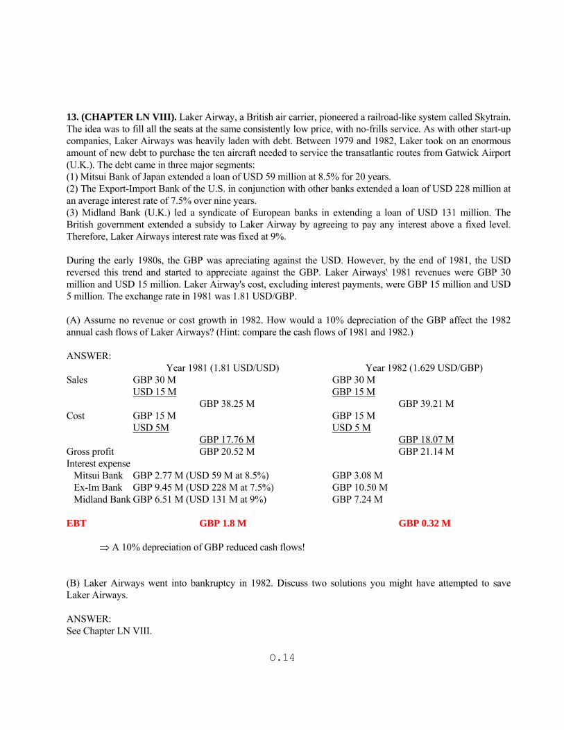
13. (CHAPTER LN VIII). Laker Airway, a British air carrier, pioneered a railroad-like system called Skytrain. The idea was to fill all the seats at the same consistently low price, with no-frills service. As with other start-up companies, Laker Airways was heavily laden with debt. Between 1979 and 1982, Laker took on an enormous amount of new debt to purchase the ten aircraft needed to service the transatlantic routes from Gatwick Airport (U.K.). The debt came in three major segments: (1) Mitsui Bank of Japan extended a loan of USD 59 million at 8.5% for 20 years. (2) The Export-Import Bank of the U.S. in conjunction with other banks extended a loan of USD 228 million at an average interest rate of 7.5% over nine years. (3) Midland Bank (U.K.) led a syndicate of European banks in extending a loan of USD 131 million. The British government extended a subsidy to Laker Airway by agreeing to pay any interest above a fixed level. Therefore, Laker Airways interest rate was fixed at 9%. During the early 1980s, the GBP was apreciating against the USD. However, by the end of 1981, the USD reversed this trend and started to appreciate against the GBP. Laker Airways' 1981 revenues were GBP 30 million and USD 15 million. Laker Airway's cost, excluding interest payments, were GBP 15 million and USD 5 million. The exchange rate in 1981 was 1.81 USD/GBP. (A) Assume no revenue or cost growth in 1982. How would a 10% depreciation of the GBP affect the 1982 annual cash flows of Laker Airways? (Hint: compare the cash flows of 1981 and 1982.) ANSWER: Year 1981 (1.81 USD/USD) Year 1982 (1.629 USD/GBP) Sales GBP 30 M GBP 30 M USD 15 M GBP 15 M GBP 38.25 M GBP 39.21 M Cost GBP 15 M GBP 15 M USD 5M USD 5 M GBP 17.76 M GBP 18.07 M Gross profit GBP 20.52 M GBP 21.14 M Interest expense Mitsui Bank GBP 2.77 M (USD 59 M at 8.5%) GBP 3.08 M Ex-Im Bank GBP 9.45 M (USD 228 M at 7.5%) GBP 10.50 M Midland Bank GBP 6.51 M (USD 131 M at 9%) GBP 7.24 M EBT GBP 1.8 M GBP 0.32 M A 10% depreciation of GBP reduced cash flows! (B) Laker Airways went into bankruptcy in 1982. Discuss two solutions you might have attempted to save Laker Airways. ANSWER: See Chapter LN VIII.

O.15

14. (CHAPTER LN XVII). You are a U.S. investor, whose U.S. portfolio tracks the U.S. market perfectly. You are considering investing in the following foreign stock markets: Market Return SD ßWORLD (%) Mexico .16 2.10 .62 U.K. .09 1.05 .84 Hong Kong .14 1.50 .49 U.S. .10 1.11 1.03 WORLD .12 1.01 1.00 RF .05 RF is the U.S. one-year Treasury Bill rate, that is, the risk free rate. ßWORLD is the beta of the foreign market with the World Index. (A) Based on a risk-adjusted performance measure (RVOL and RVAR), rank the performance of the four markets. ANSWER: RVAR RVOL Mexico .05236 .1774 UK .0381 .0476 HK .06 .1837 US .045 .05 (B) Assume you add to your U.S. portfolio, which tracks the U.S. market, all markets with a higher RVOL than the U.S. RVOL. You give a weight of 10% to each foreign market in your expanded portfolio. What is the risk of your expanded portfolio? Is the risk of your expanded portfolio lower than before? ANSWER: Add Mexico and Hong Kong. p = i i i = .80 x (1.00) + .10 x (0.62) + .10 x (0.49) = .935 (lower !)

O.16

15. (CHAPTER LN III-V). You have data on the SEK/USD and CPI indexes for Sweden and the US from January 1970 to November 1007. You run the following regression: changes in the SEK/USD exchange rate against inflation rate differentials (ISwed-IUS). Below, you have the excel regression output. 1) Let SSR(H0)= 0.37515. Test PPP, using individual t-tests and a joint F-test. 2) Let SNov = 6.326 SEK/USD, SDec = 6.3889 SEK/USD and SJan = 6.3521 SEK/USD. Suppose that you have a forecast for the inflation rates: ENov[ISwed,Dec] = .005; ENov[ISwed,Jan] = .001; ENov[IUS,Dec] = .001; ENov[IUS,Jan] = .002. Forecast the SEK/USD exchange rate in December and January, conditional on November information. 3) Using the MSE and MAE measures, is your PPP model better than the Random Walk? REGRESSION RESULTS SUMMARY OUTPUT

Regression Statistics Multiple R 0.081063264 R Square 0.006571253 Adjusted R Square 0.00431346 Standard Error 0.02901674 Observations 442

ANOVA

df SS MS F Significance

F Regression 1 0.002450538 0.002450538 2.910476709 0.088711535 Residual 440 0.370467333 0.000841971 Total 441 0.372917871

Coefficients Standard

Error t Stat P-value Lower 95% Upper 95%

Lower 95.0%

Intercept 0.00063769 0.001387156 0.459710491 0.645951097 -0.00208858 0.003364 -0.00209X Variable 1 0.42083281 0.246676358 1.706011931 0.088711535 -0.06397751 0.905643 -0.06398

1) t-stat(alpha) = [0.00063769-0]/0.001387156 = 0.459710491 < 1.96 <= cannot reject alpha=0 t-stat(beta)= [0.42083281-1]/0.246676358 = -2.347883 (|t-stat|>1.96) <= reject beta=1 F-test(H0) =((0.37515-0.37046733)/2)/(0.37046733/(440)) = 2.780776186 < 3.02 <= cannot reject H0(PPP true) 2) Et[st+1] = .0063769 + 0.42083281Et[(Id - If ) t+1] ENov [sDec] = .0063769 + 0.42083281 ENov[(ISwed – IUS )Dec] = .0063769 + 0.42083281(.005–.001) = 0.008060

O.17

ENov [SDec] =SNov (1+ENov [sDec]) = 6.326 SEK/USD x (1+0.008060) = 6.376988 SEK/USD ENov [sJan] = .0063769 + 0.42083281 ENov[(ISwed – IUS )Jan] = .0063769 + 0.42083281(.001–.002) = 0.005956 ENov [SJan] = ENov [SDec] (1+ENov [sDec]) = 6.376988 SEK/USDx (1+0.005956) = 6.414969SEK/USD 3) PPP MSE εDec= SDec - ENov[SDec] = 6.3889 SEK/USD - 6.376988 SEK/USD = 0.011912 εJan= SJan - ENov[SJan] = 6.3521 SEK/USD - 6.414969 SEK/USD = -0.062869 MSEPPP = [0.0119122 + (-0.062869)2]/2 = 0.002047 MAEPPP = [0.011912 + 0.062869]/2 = 0.037391 RW MSE εDec= SDec - SNov = 6.3889 SEK/USD - 6.326 SEK/USD = 0.062900 εJan= SJan - SDec = 6.3521 SEK/USD - 6.3889 SEK/USD = -0.036800 MSERW = [0629002 + (-0.036800)2]/2 = 0.002655 MAERW = [062900 + 0.036800]/2 = 0.049850 PPP seems better than the RW in terms of the MSE and MAE. 16. (CHAPTER LN REVIEW). You have 278 monthly observations for the MSCI Australian Index. The first six autocorrelation coefficients are: 1=.14, 2=.11, 3=.06, 4=.03, 5=-.02 and 6=.05. The Q(6) statistics is equal to 11.34 (2

6=12.59 at the 5% level). (A) Test if there any sample autocorrelation different than zero. (B) Test if the first autocorrelations are jointly significantly different than zero. (C) Looking at the size of the 's and your tests, do you have evidence that the Australian Index has autocorrelation? (A) SE=1/278 = .06 t1 = .14/.06 = 2.33 > 2; t4 = .03/.06 = 0.50 < 2 t2 = .11/.06 = 1.82 > 2; t5 = .02/.06 = 0.30 < 2 t3 = .06/.06 = 1.00 < 2; t6 = .05/.06 = 0.82 < 2 Only first order autocorrelation is significantly different from zero. (We’re approximating 1.962.) (B) Q(6)=11.34 < 2

6,.05 = 12.58 cannot reject joint insignificance at the 5% level (C) The first six autocorrelations are jointly equal to zero. The only significant autocorrelation is the first one; however, it is small. Overall, we cannot conclude that the Australian Index shows significant evidence of autocorrelation.

O.18

M1.II Long question (30 points) 1. (CHAPTER LN V) You are a U.S. investor. You have an investment of CHF 5 million in Swiss government bonds. You want to hedge CHF 5 million for six months, using monthly forward contracts. You estimate the following model for exchange rates: St = St - St-1 = as + bsSt-1 + st. Ft = Ft - Ft-1 = aF + bFFt-1 + Ft. Each element in the covariance matrix is parameterized as follows: 2

s,t = s0 + S1 e2s,t-1 + ßS1 2

s,t-1 2

F,t = F0 + S1 e2f,t-1 + ßS1 2

f,t-1 = sf,t /{f,t s,t}1/2. Suppose you estimated the above system and you got the following estimates: as=.005; bs=.35; af=.009; bf=.45; s0=.20; s1=.15; ßs1=.80;f0=.30; f1=.20; ßf1=.75; =.75. You are given the following data: spot and 30-day forward rates (USD/CHF) for the months of August, September, October, and November. SAug=.952; SSep=.940; SOct=.934; SNov=.925; FAug=.947; FSep=.940; FOct=.936; FNov=.924; 2

s,Oct=.430; 2f,Oct=.410.

At the end of October, you constructed your hedge ratio (hNov= -sf,t=Nov/2

f,t=Nov). (A) Now, at the end of November, you are required to construct your hedge ratio for December, that is you want hDec. ANSWER: St S,t 2

S,t Ft F,t 2F,t SF,t ht

September -.012 .----. .----. -.007 .-----. .-----. .----. .----. October -.006 -.0068 .430 .004 -.00985 .410 .3267 -.7681 November -.009 -.0119 .5440 -.012 -.01920 .6075 .4263 -.7097 December ... ... .6352 .7557 .5196 -.6876 That is, the hedge ratio for December is -.6876. (B) Interpret the hedge ratio for December, hDec. ANSWER: For each CHF long, we need to have CHF .69 short.

O.19

(C) The CHF/USD forward contract size is CHF 125,000. (i) Do you need to buy or sell forward contracts? (ii) How many contracts do you need to hedge your position? ANSWER: (i) Underlying position: Long CHF 5,000,000. sell forward CHF contracts (ii) Number of contracts = CHF 5,000,000 x (-.69)/CHF 125,000 = -27.6 contracts 28 contracts.

O.20

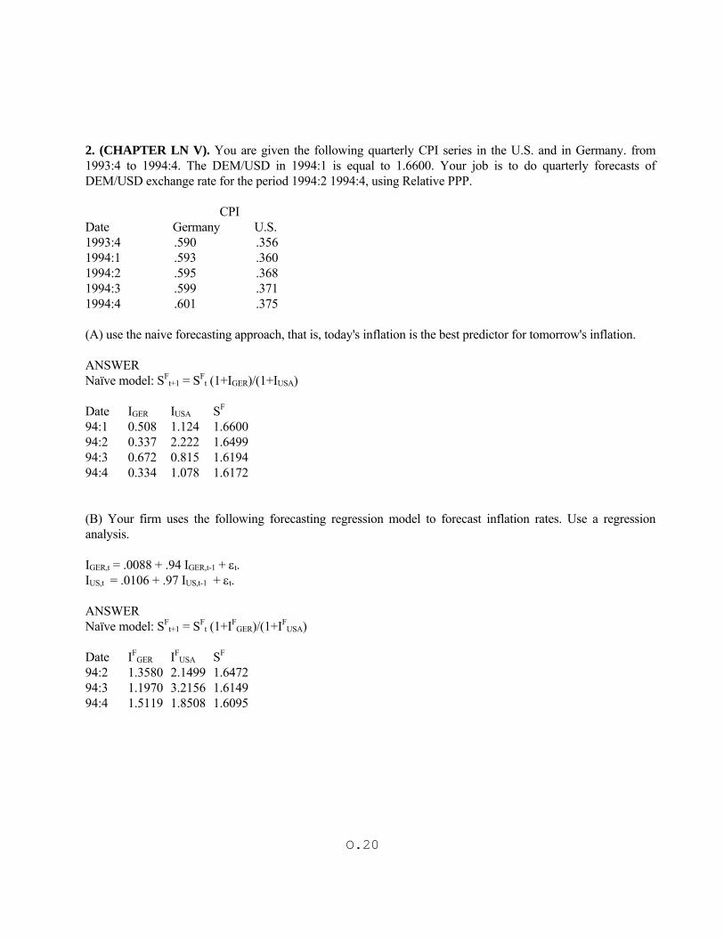
2. (CHAPTER LN V). You are given the following quarterly CPI series in the U.S. and in Germany. from 1993:4 to 1994:4. The DEM/USD in 1994:1 is equal to 1.6600. Your job is to do quarterly forecasts of DEM/USD exchange rate for the period 1994:2 1994:4, using Relative PPP. CPI Date Germany U.S. 1993:4 .590 .356 1994:1 .593 .360 1994:2 .595 .368 1994:3 .599 .371 1994:4 .601 .375 (A) use the naive forecasting approach, that is, today's inflation is the best predictor for tomorrow's inflation. ANSWER Naïve model: SF

t+1 = SFt (1+IGER)/(1+IUSA)

Date IGER IUSA SF 94:1 0.508 1.124 1.6600 94:2 0.337 2.222 1.6499 94:3 0.672 0.815 1.6194 94:4 0.334 1.078 1.6172 (B) Your firm uses the following forecasting regression model to forecast inflation rates. Use a regression analysis. IGER,t = .0088 + .94 IGER,t-1 + t. IUS,t = .0106 + .97 IUS,t-1 + t. ANSWER Naïve model: SF

t+1 = SFt (1+IF

GER)/(1+IFUSA)

Date IF

GER IFUSA SF

94:2 1.3580 2.1499 1.6472 94:3 1.1970 3.2156 1.6149 94:4 1.5119 1.8508 1.6095

O.21

3. (CHAPTER V). You work in Hong Kong for a local investment bank. You have available quarterly interest rate series in the U.S., CPIUSD, and in Hong Kong, CPIHKD, from 2001:4 to 2002:3. You also have available GDP indexes (GDP) for the U.S. and Hong Kong. The HKD/USD in 2002:1 was equal to 7.400.Your job is to do quarterly forecasts of the HKD/USD exchange rate for the period 2002:2-2001:4, using the following model: St+1/St = 1 + .5 (id,t+1 - if,t+1) + .5 (yf,t+1 - yd,t+1). This model is a mixture of IFE and the monetary approach. You have the following data: Date GDPHKD GDPUSD Forecast (SF) Actual St iHKD-iUSD

2001:4 2160 3150 7.155 7.155 .0150 2002:1 2330 3220 7.400 7.400 .0205 2002:2 2490 3370 7.450 .0180 2002:3 2620 3410 7.500 .0240 2002:4 7.600 To forecast income growth rates your firm uses the following regression model: yHKD,t = .004 + .85 yHKD,t-1 + HKD,t. yUSD,t = .003 + .90 yUSD,t-1 + USD,t. To forecast interest rates (i) your firm uses a naive approach -i.e., today’s interest rate is the best predictor for tomorrow’s interest rate. (A) Your job is to do quarterly forecasts of HKD/USD exchange rate for the period 2002:2-2002:4. (B) Use the forward rate to forecast the HKD/USD exchange rate for the period 2002:2-2002:4. (C) Use the random walk to forecast the HKD/USD exchange rate for the period 2002:2-2002:4. (D) Compare your forecasts from (A), (B) and (C). (Hint: calculate MAE for each model) (E) Suppose your firm is long USD 100,000,000. According to your forecasts in (A) and (B), would you hedge this exposure? ANSWER: (A) Use ad-hoc model to forecast St. First, you need to forecast yt+1(yF

t+1). yF

HKD,2002:2 = .004 + .85 x. 0.0787 = 0.0709 yF

USD,2002:2 = .003 + .90 x. 0.0222 = 0.0230 SF

t+1 = SFt [1 + .5 (id,t - if,t) + .5 (yF

f,t+1 – yFd,t+1)] = 7.4 x [1+.5x(.205)+.5x(.0230-.0709)] = 7.2986

2002:2 = SF2002:2-S2002:2 = 7.2986 – 7.4500 = -01514

Date yF

HKD yFUSD Forecast (SF) Actual St Forecast Error

2002:2 .0709 .0230 7.2986 7.450 -0.1514 2002:3 .0624 .0449 7.3007 7.500 -0.1993 2002:4 .0484 .0137 7.2616 7.600 -0.3384

O.22

(B) Use IRP to calculate forward rates. SF t+1 = Ft,90 = St [1 + (id,t - if,t)x90/360] = 7.4 HKD/USD x [1+(.205)x90/360] = 7.4379 HKD/USD 2002:2 = SF

2002:2-S2002:2 = 7.4379 – 7.4500 = -0121 Date Forecast (SF) Actual St Forecast Error

2002:2 7.4379 7.450 -0.0121 2002:3 7.4835 7.500 -0.0165 2002:4 7.5450 7.600 -0.0550 (C) SF t+1 = St = 7.400 HKD/USD. 2002:2 = SF

2002:2-S2002:2 = 7.400 – 7.4500 = -0050 Date Forecast (SF) Actual St Forecast Error

2002:2 7.400 7.450 -0.0500 2002:3 7.450 7.500 -0.0500 2002:4 7.500 7.600 -0.1000 (D) MAE (Ad-hoc) = 0.2297 MAE (FR) = 0.0278 MAE (RW) = 0.0667 The forward rate model is the best forecasting model, according to the mean absolute error measure. (F) According to A, the firm should hedge since an appreciation of the HKD against the USD is forecasted. According to B, the firm should not hedge since a depreciation of the HKD against the USD is forecasted.