appendix n pipeline design approach -...
TRANSCRIPT

Alaska Stand Alone Gas Pipeline Final EIS
Appendix N
Pipeline Design Approach


Alaska Stand Alone Gas Pipeline Final EIS
Appendix N
Pipeline Design Approach


© 2011 AGDC. All rights reserved. This material is copyrighted and contains proprietary information. Neither the document nor the information contained within it may be reproduced, displayed, modified or distributed without the express prior written permission of AGDC. For permission, contact [email protected] or AGDC, P.O. Box 101020, Anchorage, Alaska 99510.
Michael Baker Jr., Inc. 6/9/2011
121283-MBJ-RPT-024 Rev. 0
Alaska Stand Alone Gas Pipeline / ASAP
Design Methodology to Address Frost Heave Potential
Prepared for:


Alaska Stand Alone Gas Pipeline/ASAP Design Methodology to Address Frost Heave Potential Rev. 0 June 9, 2011
Michael Baker Jr., Inc. 121283-MBJ-RPT-024 Page iii Proprietary
EXECUTIVE SUMMARY
The purpose of this report is to introduce the design methodology for addressing potential threats related to frost heave in areas where the ASAP is routed through frost susceptible soils. Specifically, this report introduces the ASAP approach to the structural mechanics issues of the pipeline, particularly the methodology employed to ensure pipeline mechanical structural integrity when subjected to potential displacements associated with earth movement.
The report also addresses questions raised by the Pipeline and Hazardous Materials Safety Administration (PHMSA) to the Alaska Gasline Development Corporation (AGDC) regarding the approach to structural mechanics of the Alaska Stand Alone Gas Pipeline/ASAP (ASAP) relating to potential ditch displacements, such as frost heave, which could affect the longitudinal stress/strain response of the pipeline.
The ASAP project methodology to ensure pipeline integrity from time-dependent threats such as frost heave depends on the evaluation of a limiting curvature of the pipe. The limiting curvature of the pipe is used for design screening of the route terrain units and developing operational monitoring using pipeline in-line inspection (ILI) tools that detect pipeline movement (e.g., high resolution geometry pigs). The limiting curvature criterion is derived from consideration of limiting tensile and compressive strains capacities of the pipe material. This criterion is used to screen pipe route segments which do not exceed the criteria limits, after evaluation of the interaction of the pipe material, its operating characteristics, and the segment route subsurface behavior. Those segments that are determined to potentially exceed the curvature criteria limits are subject to mitigative actions to reduce the pipe response to within acceptable bounds.
Section 1 through Section 4 introduce the ASAP design terminology as it applies to this effort. In particular, these chapters relate the development of the methodology that employs curvature limits to ensure pipeline integrity, especially for those displacement-controlled loadings that induce transverse bending. The introductory material includes background on the determination of the loading, its associated soil and pipe resisting functions, and how these are integrated in a combined pipe-soil interaction analysis. The analytical process measures the effect of the loading and soil resisting functions on pipe response against quantitative structural integrity criteria for the range of route soils to be encountered and a range of operational conditions. This evaluation process for the range of alignment conditions forms the demand evaluation.
Section 5 focuses on the line pipe material and fabrication, and the corresponding development of appropriate design limits using these materials. These limits are used as the capacity evaluation and are used to judge the acceptance or rejection of the demand developed in the previous chapters. Section 5 then addresses the questions:
• How are the curvature limits to be developed? • What tests will be conducted to verify the limits? • What material requirements will be imposed?
Section 6 outlines the application of the design methodology to the alignment. This includes an introduction to the alignment conditions where the loading under consideration in this report, frost heave, would not occur. The application methodology is presented as a progressive exclusion sieve, narrowing

Alaska Stand Alone Gas Pipeline/ASAP Design Methodology to Address Frost Heave Potential Rev. 0 June 9, 2011
Michael Baker Jr., Inc. 121283-MBJ-RPT-024 Page iv Proprietary
down the alignment conditions, and associated alignment geographical segments, where the concern needs more detailed evaluation and potential mitigation. This chapter addresses the questions:
• Where would curvature criteria be used? • Where would curvature criteria not be used?
Section 7 addresses construction requirements relating to frost heave answering the question:
• What modifications to standard construction techniques will be needed?
Section 8 addresses potential operational mitigation methods if operational monitoring concludes that the established curvature/strain limits may be exceeded and pipeline integrity is at risk. This chapter addresses the questions:
• What monitoring will be required during operations to ensure the limits are not exceeded? • What mitigation measures will be employed should the limits be approached or exceeded?
As discussed with PHMSA, AGDC has not yet developed the final quantitative criteria, nor has AGDC compiled the ASAP alignment subsurface evaluation, which would allow completion of this design determination and application of the frost heave methodology to final design. Nevertheless, AGDC is confident that the process presented herein addresses the design methodology requirements needed at this front end of preliminary design, and forms a framework for successful evaluation of the route in final design.

Alaska Stand Alone Gas Pipeline/ASAP Design Methodology to Address Frost Heave Potential Rev. 0 June 9, 2011
Michael Baker Jr., Inc. 121283-MBJ-RPT-024 Page v Proprietary
CONTENTS
Executive Summary .............................................................................................................................................. iii
Acronyms and Abbreviations ............................................................................................................................... vii
Section 1. Introduction ...................................................................................................................................... 1 1.1 Project Overview .......................................................................................................................................... 1 1.2 Project Phasing and Associated Deliverables ............................................................................................... 4
1.2.1 Project Phasing .................................................................................................................................... 4 1.2.2 Design Deliverables ............................................................................................................................. 5
1.3 Organization of the Report ........................................................................................................................... 7
Section 2. Structural Mechanics of Buried Pipelines .......................................................................................... 8 2.1 Pressure Containment .................................................................................................................................. 9 2.2 Treatment of Longitudinal Loadings ........................................................................................................... 10 2.3 Effective Stress ........................................................................................................................................... 11 2.4 Application of the Methodology ................................................................................................................. 13
Section 3. Geohazards ..................................................................................................................................... 14 3.1 Geothermal Considerations ........................................................................................................................ 14 3.2 Design Development .................................................................................................................................. 16
3.2.1 Geotechnical/Geothermal Data ........................................................................................................ 16 3.2.2 Selection of Geotechnical/Geothermal Parameters for Design ........................................................ 16
3.3 Application of the Methodology ................................................................................................................. 19
Section 4. Strain Demand Determination ........................................................................................................ 20 4.1 Pipe-Soil Interaction Analysis Overview ..................................................................................................... 20 4.2 Pipe Material Properties ............................................................................................................................. 22 4.3 Geothermal Input ....................................................................................................................................... 23 4.4 Soil Resistance Characterization ................................................................................................................. 26
4.4.1 Uplift resistance ................................................................................................................................. 27 4.4.2 Bearing Resistance ............................................................................................................................. 28 4.4.3 Longitudinal Resistance ..................................................................................................................... 28
4.5 Model geometry ......................................................................................................................................... 29 4.6 Imposed Loads ............................................................................................................................................ 29
Section 5. Strain Capacity Determination ........................................................................................................ 32 5.1 Material Requirements ............................................................................................................................... 32
5.1.1 Line Pipe ............................................................................................................................................ 32 5.1.2 Coating Effect .................................................................................................................................... 35 5.1.3 Dimensional Control .......................................................................................................................... 36 5.1.4 Girth Welds ........................................................................................................................................ 36 5.1.5 Weld Overmatch ................................................................................................................................ 36 5.1.6 Weldment Toughness ........................................................................................................................ 36
5.2 Testing Requirements ................................................................................................................................. 37 5.2.1 Curved Wide Plate Testing ................................................................................................................ 37 5.2.2 Full-Scale Tension Testing .................................................................................................................. 37 5.2.3 Compressive Strain Validation ........................................................................................................... 38
Section 6. Route Application ........................................................................................................................... 39 6.1 Design Approach ......................................................................................................................................... 39 6.2 Segment-by-Segment Design...................................................................................................................... 39 6.3 Potential Design Mitigative measures ........................................................................................................ 41
Section 7. Construction Related Issues ............................................................................................................ 42

Alaska Stand Alone Gas Pipeline/ASAP Design Methodology to Address Frost Heave Potential Rev. 0 June 9, 2011
Michael Baker Jr., Inc. 121283-MBJ-RPT-024 Page vi Proprietary
7.1 Welding Procedures ................................................................................................................................... 42 7.2 Automated Ultrasonic Testing .................................................................................................................... 42
Section 8. Operations and Maintenance .......................................................................................................... 43 8.1 Monitoring Potential Frost Heave .............................................................................................................. 43 8.2 Potential Operational Mitigative measures ................................................................................................ 44
8.2.1 Temperature Control ......................................................................................................................... 44 8.2.2 Line Leveling ...................................................................................................................................... 45
Section 9. Conclusion ...................................................................................................................................... 46
Section 10. References ...................................................................................................................................... 47
Appendix A PHMSA Correspondence ................................................................................................................ A.1
Appendix B Structural Mechanics of Buried Pipelines ....................................................................................... B.1
TABLES
Table 3.1 U.S. Army Corps of Engineers Frost Design Soil Classification System ................................................... 17 Table 3.2 Geotechnical Tests for Frost Heave Potential ........................................................................................ 18 Table 3.3 Additional Geotechnical Tests for Frost Heave Evaluation .................................................................... 18
FIGURES
Figure 1.1 Route Map ................................................................................................................................................ 3 Figure 1.2 Project Schedule ....................................................................................................................................... 4 Figure 1.3 Design Approach Flowchart ..................................................................................................................... 6 Figure 2.1 Illustration of Tresca and von Mises Yield Functions ............................................................................. 12 Figure 3.1 ASAP Permafrost Characteristics ............................................................................................................ 15 Figure 4.1 Frost Heave Illustration .......................................................................................................................... 21 Figure 4.2 Frost Bulb Schematic .............................................................................................................................. 24 Figure 4.3 Illustration of Maximum Curvature Time History .................................................................................. 31 Figure 5.1 Normative Properties of a Steel Stress-Strain Relationship ................................................................... 33 Figure 5.2 Illustration of Differing Stress-Strain Behavior in the Knee Region........................................................ 34 Figure 6.1 Frost Heave Route Assessment Flow Chart ............................................................................................ 40

Alaska Stand Alone Gas Pipeline/ASAP Design Methodology to Address Frost Heave Potential Rev. 0 June 9, 2011
Michael Baker Jr., Inc. 121283-MBJ-RPT-024 Page vii Proprietary
ACRONYMS AND ABBREVIATIONS ADOT&PF Alaska Department of Transportation and
Public Facilities AGDC Alaska Gasline Development Corporation API American Petroleum Institute APSC Alyeska Pipeline Service Company ARRC Alaska Railroad Corporation ASAP Alaska Stand Alone Gas Pipeline ASME American Society of Mechanical Engineers ASTM American Standard Testing Materials AUT Automated ultrasonic testing BLM Bureau of Land Management cf Cubic feet CFR Code of Federal Regulations CO2 Carbon dioxide CTOD Crack tip opening displacement D/t Diameter to wall thickness ratio DGGS State of Alaska Division of Geological and
Geophysical Surveys FEL Front end loading GIS Geographic Information System HDD Horizontal directional drill(ing) HT Hoop tension ILI In-Line Inspection INS Inertial Navigation System ksi Kips per square inch LT Longitudinal tension MAOP Maximum allowable operating pressure MMscfd Million standard cubic feet per day PHMSA Pipeline and Hazardous Materials Safety
Administration psi Pounds per square inch psig Pounds per square inch gage ROW Right-of-way SMYS Specified minimum yield strength TAPS Trans-Alaska Pipeline System U.S. United States of America UAF University of Alaska Fairbanks USGS U.S. Geological Survey

Alaska Stand Alone Gas Pipeline/ASAP Design Methodology to Address Frost Heave Potential Rev. 0 June 9, 2011
Michael Baker Jr., Inc. 121283-MBJ-RPT-024 Page 1
Section 1 Proprietary Introduction
SECTION 1. INTRODUCTION
The purpose of this report is to introduce the design methodology for addressing potential threats related to frost heave in areas where the ASAP is routed through frost susceptible soils. Specifically, this report introduces the ASAP approach to the structural mechanics issues of the pipeline, in particular the methodology employed to ensure pipeline mechanical structural integrity when subjected to potential displacements associated with earth movement.
Presentation of the design methodology will help address questions raised by the Pipeline and Hazardous Materials Safety Administration (PHMSA) in correspondence to the Alaska Stand Alone Gas Pipeline/ASAP project (ASAP or the Project) and in meetings between PHMSA and the ASAP technical team. Correspondence with PHMSA is reproduced in Appendix A of this report. The specific item of interest is the section entitled “External loads that exceed design allowable – strain based design” contained in the letter to Dan Fauske from Jeffrey Wiese, received by the Alaska Gasline Development Corporation (AGDC) on May 4, 2011. In the beginning of this section, five code segments of the federal regulations are cited: 49 CFR 192, paragraphs 192.103, 192. 105, 192.111, 192.317, and 192.620. Further discussion of these regulations is presented in Section 2.
Potential threats to the pipeline integrity are generally identified and assessed using ASME B31.8S, Managing System Integrity of Gas Pipelines, which has an overview of a generalized procedure to the approach to earth movement threats contained in Section A-9, “Weather Related and Outside Force Threat (Earth Movement, Heavy Rains or Floods, Cold Weather, Lightning).” The potential pipeline displacement loading from earth movement used to illustrate the approach in this report is frost heave. Note that frost heave is a time-dependent threat, which is different from other familiar earth movement threats, such as seismicity, which are time-independent.
1.1 PROJECT OVERVIEW
The purpose of the Alaska Stand Alone Gas Pipeline/ASAP is to provide the in-state infrastructure for the reliable delivery of natural gas, primarily from the existing gas production facilities on the North Slope of Alaska, to markets in South Central Alaska, Fairbanks, and other communities, as practical. The pipeline routing is generally along the state’s existing highway corridors from the North Slope to tidewater in Southcentral Alaska. A route map is presented in Figure 1.1.
The design basis for ASAP consists of a 24-inch-diameter chilled natural gas pipeline, approximately 737 miles in length, with a flow rate of up to 500 million standard cubic feet per day (MMscfd). The mainline pipeline system will be designed to transport natural gas consisting of either a highly-conditioned natural gas enriched in non-methane hydrocarbons or of conditioned natural gas containing mostly methane. At the 500 MMscfd throughput a single compressor station is required to be located approximately 286 miles south of Prudhoe Bay. A 12-inch lateral pipeline, approximately 35 miles in length, will tie-in to the mainline at approximately ASAP milepost 458 to supply up to 60 MMscfd of utility grade gas to Fairbanks.
The majority of the pipeline will be installed belowground utilizing conventional trenching techniques. The mainline pipeline will be API 5L X70 pipe with a minimum wall thickness of 0.595 inches, for the maximum allowable operating pressure (MAOP) of 2500 psig, which corresponds to

Alaska Stand Alone Gas Pipeline/ASAP Design Methodology to Address Frost Heave Potential Rev. 0 June 9, 2011
Michael Baker Jr., Inc. 121283-MBJ-RPT-024 Page 2
Section 1 Proprietary Introduction
a design factor of 0.72. There is no intention of utilizing the alternative MAOP provisions of the 49 CFR 192 regulations which allow an increase of the design factor to 0.80. Since much of the pipe lies within the state roadway right-of-way (ROW), the design factor for over half the length of the mainline is 0.60 resulting in a wall thickness increase to 0.714 inches. The decrease in the design factor is required so as to conform to the 49 CFR 192.111(b)(2) when the pipeline is in a parallel encroachment. The Fairbanks Lateral will be API 5L X65 pipe with a minimum wall thickness of 0.250 inches (increased from 0.190 inches for constructability) for the MAOP of 1480 psig.

Alaska Stand Alone Gas Pipeline/ASAP Design Methodology to Address Frost Heave Potential Rev. 0 June 9, 2011
Michael Baker Jr., Inc. 121283-MBJ-RPT-024 Page 3
Section 1 Proprietary Introduction
Figure 1.1 Route Map

Alaska Stand Alone Gas Pipeline/ASAP Design Methodology to Address Frost Heave Potential Rev. 0 June 9, 2011
Michael Baker Jr., Inc. 121283-MBJ-RPT-024 Page 4
Section 1 Proprietary Introduction
1.2 PROJECT PHASING AND ASSOCIATED DELIVERABLES
1.2.1 PROJECT PHASING
Research shows that the disciplined application of a stage-gated process is strongly correlated with producing superior project outcomes. The gated approach involves breaking a capital project into discretely defined phases, where a clear set of deliverables or outcomes is outlined for each phase, which must be completed before the project is approved to move into the next phase. AGDC will be employing a stage-gated approach to project execution and delivery.
The first major phase of the gated project delivery process is FEL (front-end loading). Three stages usually comprise the FEL process (Conceptual Engineering, Preliminary Design, and Detailed Design) prior to project sanction (start of Execution). ASAP is currently in Conceptual Engineering, or early definition stages of project development.
The results of the initial phases provide critical input for making the final authorization decision to move forward with the project. The primary objective of FEL is to achieve an understanding of the project that is sufficiently detailed so that significant and costly changes in engineering, construction, and the startup phases of a project will be minimized.
The Conceptual Engineering project objective is development of the Project Plan due July 1, 2011. This will be the end of Conceptual Engineering. After that time, the Alaska Legislature will decide whether the Project will proceed to Preliminary Design, utilizing State funding, or whether the Project will be shelved or in some way modified at the end of the funding period in July 2011.
As the Project progresses into Preliminary Design and beyond, development of a large integrated project team will be needed comprised of people with a wide range of capabilities that can perform key functional roles in the project team organization. Project skill sets that will be required to move the project forward include operations, maintenance, business, process design, project controls, construction management, procurement and contracting, quality assurance, health and safety, and permitting.
Figure 1.2 Project Schedule

Alaska Stand Alone Gas Pipeline/ASAP Design Methodology to Address Frost Heave Potential Rev. 0 June 9, 2011
Michael Baker Jr., Inc. 121283-MBJ-RPT-024 Page 5
Section 1 Proprietary Introduction
1.2.2 DESIGN DELIVERABLES
The frost heave design approach is depicted in Figure 1.3 and will be explained further throughout this report. As the design progresses from Preliminary Design though Detailed Design and then Construction, information is being collated and verified to allow the design to progress along this design approach flowchart. In general, Preliminary Design follows the methodology development, scopes the data collection required for the demand and capacity to be further verified, and starts the data development for the route. Tasks scheduled to be finalized in Preliminary Design include:
• Identification of the input parameters required for the project approach that will implement this design methodology, including the analysis of the geothermal conditions and the structural analysis.
• Trial analyses completed and documented. • The terrain units along the identified alignment are identified and captured in the project
GIS – appropriate geotechnical parameters identified as required input for the methodology are assigned to the terrain units based on borehole analysis.
• The alignment route geo-database is implemented within the project GIS, concentrating on the subsurface information available along the routes from past exploratory tasks.
• Gaps in the route geo-database will be identified for required exploration. • Potential manufacturers of the line pipe are contacted, and joints of the line pipe acquired
for small-scale testing to be completed before the end of Preliminary Design.
Detailed Design will include finalizing the capacity and demand-capacity application evaluation process for the route including the following tasks:
• Finalization of the frost heave design approach methodology. • The line pipe strain capacity is determined using the small-scale test results, and verified
with full-scale testing. • The route geo-database will be queried using the design methodology with route segments
displaying potential unallowable heave potential subjected to additional scrutiny and/or mitigative measures.
• The final material and pipe order will incorporate any requirements to implement these measures.
The identified potential line segments subject to additional scrutiny identified in final design may require special mitigative measures that could be the basis of a special construction team. Baseline monitoring will be required within a practicable time after startup, followed with operational monitoring throughout the life of the project.
Design reviews by PHMSA and other agencies will occur throughout the various phases of the project.

Alaska Stand Alone Gas Pipeline/ASAP Design Methodology to Address Frost Heave Potential Rev. 0 June 9, 2011
Michael Baker Jr., Inc. 121283-MBJ-RPT-024 Page 6
Section 1 Proprietary Introduction
Figure 1.3 Design Approach Flowchart
NO
YES
QA/QC Program
Operations • Monitoring • Mitigation
Monitoring and Mitigation
Criteria
Construction • Geotechnical Verification • Construction Mitigation
Finalize Design
Capacity >
Demand
Perform Pipe-Soil Structural
Modeling
Perform Materials Testing
Frost Heave and Thaw
Settlement
Perform Geothermal and
Hydraulic Analyses
Perform FEA Simulations
Develop and Qualify Pipe and Weld Properties
Select Pipe Grade and Wall
Thickness
Collect Route Soils/Geohazard
Data
Refine Route Data and Material Requirements
Set Strain Demand Limits
Set Strain Capacity Limits

Alaska Stand Alone Gas Pipeline/ASAP Design Methodology to Address Frost Heave Potential Rev. 0 June 9, 2011
Michael Baker Jr., Inc. 121283-MBJ-RPT-024 Page 7
Section 1 Proprietary Introduction
1.3 ORGANIZATION OF THE REPORT
Section 1 through Section 4 introduce the ASAP design terminology as it applies to this effort. In particular, these chapters relate the development of the methodology that employs curvature limits to ensure pipeline structural integrity especially for those displacement-controlled loadings that induce transverse bending. The introductory material includes background on the determination of the loading, its associated soil and pipe resisting functions, and how these are integrated in a combined pipe-soil interaction analysis. The analytical process measures the effect of the loading and soil resisting functions on pipe response against quantitative structural integrity criteria for the range of route soils to be encountered as well as a range of operational conditions. This evaluation process for the range of alignment conditions forms the demand evaluation.
Section 5 focuses on the line pipe material and fabrication, and the corresponding development of appropriate design limits using these materials. These limits are used as the resistance capacity and are used to judge the acceptance or rejection of the demand developed in the previous chapters. Section 5 then addresses the questions:
• How are the curvature limits to be developed? • What tests will be conducted to verify the limits? • What material requirements will be imposed?
Section 6 outlines the application of the design methodology to the alignment. This includes an introduction to the alignment conditions where the loading under consideration in this report, frost heave, would not occur. The application methodology is presented as a progressive exclusion sieve, narrowing down the alignment conditions, and associated alignment geographical segments, where the concern needs more detailed evaluation and potential mitigation. This chapter addresses the questions:
• Where would curvature criteria be used? • Where would curvature criteria not be used?
Section 7 addresses construction requirements relating to frost heave answering the question:
• What modifications to standard construction techniques will be needed?
Section 8 addresses potential operational mitigative methods if operational monitoring concludes that the established limits may be exceeded and pipeline integrity is at risk. This chapter addresses the questions:
• What monitoring will be required during operations to ensure the limits are not exceeded? • What mitigation measures will be employed should the limits be approached or exceeded?
Alaska Stand Alone Gas Pipeline/ASAP Design Methodology to Address Frost Heave Potential Rev. 0 June 9, 2011
Michael Baker Jr., Inc. 121283-MBJ-RPT-024 Page 8
Section 2 ProprietaryStructural Mechanics of Buried Pipelines
SECTION 2. STRUCTURAL MECHANICS OF BURIED PIPELINES
Although some sections of the ASAP are aboveground, notably at waterway crossings and at the beginning of pipeline route on the North Slope, ASAP is primarily a buried pipeline. Buried pipelines are essentially “restrained,” that is, displacement of the pipe is restricted by the soil around it.
For the problem of frost heave, advanced analytical tools, and input functions needed to characterize the components of the frost heave methodology, are required to integrate the various parts of the loading and resistance functions so as to correctly address the loading demand on the pipeline. This section reviews some of the familiar parts of the demand problem, such as the internal pressure and change in temperature, and then reviews how these are integrated into the time-dependent loading functions for the longitudinal stress components to derive a unified mechanical approach.
The basis of the structural mechanics for pipeline engineering is summarized in Appendix B. For such a straightforward “structure,” a pressurized pipe can actually exhibit fairly complex behavior involving significant stress components in a biaxial stress state.
The resultant mechanical state of the pipeline that arises from the external loads imposed from different sources, causing both hoop and longitudinal pipe stress effects, is referred to as the “demand” on the pipeline. Since the overall resultant is a complex stress state, the demand is best characterized in this combined state – i.e., because the relative magnitudes of the orthogonal components are roughly of the same magnitude, the interaction mechanics must be considered.
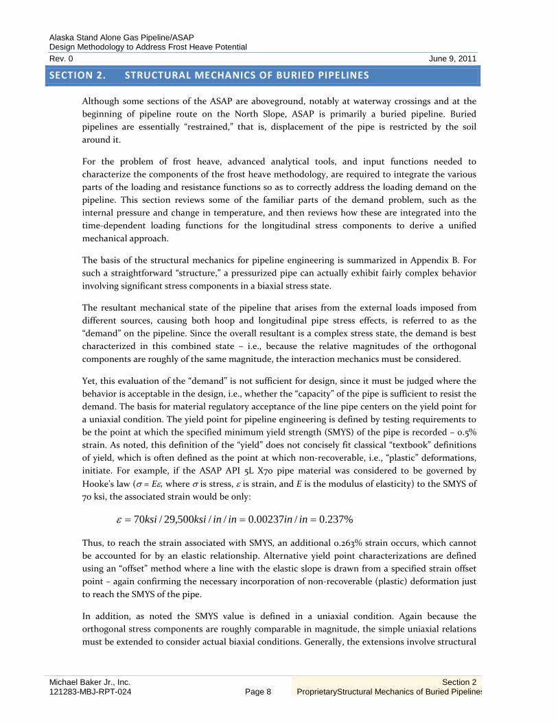
Yet, this evaluation of the “demand” is not sufficient for design, since it must be judged where the behavior is acceptable in the design, i.e., whether the “capacity” of the pipe is sufficient to resist the demand. The basis for material regulatory acceptance of the line pipe centers on the yield point for a uniaxial condition. The yield point for pipeline engineering is defined by testing requirements to be the point at which the specified minimum yield strength (SMYS) of the pipe is recorded – 0.5% strain. As noted, this definition of the “yield” does not concisely fit classical “textbook” definitions of yield, which is often defined as the point at which non-recoverable, i.e., “plastic” deformations, initiate. For example, if the ASAP API 5L X70 pipe material was considered to be governed by Hooke’s law (σ = Eε, where σ is stress, ε is strain, and E is the modulus of elasticity) to the SMYS of 70 ksi, the associated strain would be only:
%237.0/00237.0//500,29/70 === ininininksiksiε
Thus, to reach the strain associated with SMYS, an additional 0.263% strain occurs, which cannot be accounted for by an elastic relationship. Alternative yield point characterizations are defined using an “offset” method where a line with the elastic slope is drawn from a specified strain offset point – again confirming the necessary incorporation of non-recoverable (plastic) deformation just to reach the SMYS of the pipe.
In addition, as noted the SMYS value is defined in a uniaxial condition. Again because the orthogonal stress components are roughly comparable in magnitude, the simple uniaxial relations must be extended to consider actual biaxial conditions. Generally, the extensions involve structural

Alaska Stand Alone Gas Pipeline/ASAP Design Methodology to Address Frost Heave Potential Rev. 0 June 9, 2011
Michael Baker Jr., Inc. 121283-MBJ-RPT-024 Page 9
Section 2 ProprietaryStructural Mechanics of Buried Pipelines
mechanics relationships that allow the combined stress conditions to be related back to uniaxial tests and uniaxial stress conditions or “effective” stresses that characterize the biaxial conditions, often by reference to a skewed reference frame.
2.1 PRESSURE CONTAINMENT
The governing regulatory document for the ASAP pipeline, 49 CFR 192, addresses the “…design pressure for steel pipe…” in 49 CFR 192.105. The design factor used in this formula for the design pressure is addressed in 49 CFR 192.111.
Although there are provisions for alternative approaches to this design factor, with additional associated requirements for utilizing this alternative formulation, AGDC has elected to everywhere avoid this alternative formulation for the design factor. Thus, requirements relating to this alternative formulation, including those cited in 49 CFR 192.620, are not applicable to ASAP and are not further addressed in this report.
The design pressure formula cited in the federal regulations (P = (2 St/D)×F×E×T) is recognized as the classical Barlow’s formula derived from basic equilibrium considerations (see Appendix B). The derivation does not depend on the material type (e.g., steel, aluminum, etc.), the mechanical state of the pipe material (elastic, inelastic, plastic…) nor consideration of pipe behavior in the orthogonal longitudinal direction. The robustness of this formulation makes it ideal for the focus of pressure containment guidance, both in regulations and consensual standards.
On the other hand, and somewhat because there are no associated limiting conditions arising from the derivation for the application of this formula, there are no associated explicit requirements for other types of loadings that can be deduced from this design pressure formula. In particular, there are no requirements associated with the design pressure formula that impose any conditions or limitations upon the longitudinal stress/strain behavior of the pipeline. There are more exact formulations for thick-walled pipes (generally defined as having a diameter to wall thickness ratio (D/t) of less than 20), but typical transmission lines, including ASAP, are thin-walled pipes.
Thus, the design pressure formula cited in the regulations will be met regardless of the design limitations imposed on the longitudinal effects, i.e., if the pipeline diameter, thickness, and operating pressure meet a 72% specified minimum yield strength (SMYS) requirement at startup, the same combination of these input parameters into the design pressure formula cited in the regulations will produce the same limiting stress of 72% SMYS, and thus identically meet these regulatory requirements indefinitely throughout operations, regardless of the longitudinal behavior. This is a conclusion from the stress mechanics of pipelines, and is not peculiar to any aspect of the ASAP nor to any transmission pipeline.

Alaska Stand Alone Gas Pipeline/ASAP Design Methodology to Address Frost Heave Potential Rev. 0 June 9, 2011
Michael Baker Jr., Inc. 121283-MBJ-RPT-024 Page 10
Section 2 ProprietaryStructural Mechanics of Buried Pipelines
2.2 TREATMENT OF LONGITUDINAL LOADINGS
In contrast to the explicit requirements for the design pressure formula, the federal regulations contain only general guidance for additional types of loadings, and no explicit limitations. General guidance is contained in 49 CFR 192.103 which states:
Pipe must be designed with sufficient wall thickness, or must be installed with adequate protection, to withstand anticipated external pressures and loads that will be imposed on the pipe after installation.
More specifics about potential hazards to be investigated are contained in 192.317:
(a) The operator must take all practicable steps to protect each transmission line or main from washouts, floods, unstable soil, landslides, or other hazards that may cause the pipeline to move or to sustain abnormal loads…
If additional thickness is found to be required for reasons other than pressure containment, the allowable pressure must not be increased through a re-computation of the design pressure formula to take advantage of this additional thickness as per 49 CFR 192.105.
The requirements of 49 CFR 192 quoted above, though general in nature, are an explicit reminder to all operators that prudent oversight of the potential detrimental effects from external loads requires diligent investigation and cannot be waived. To satisfy this requirement, the pipeline industry has addressed the lack of explicit requirements in the regulatory framework through consensual standards so as to satisfy the general regulatory requirements.
The U.S. gas industry accepted standard for requirements in areas where the regulations give only general guidance is ASME B31.8, Gas Transmission and Distribution Piping Systems. To be clear, where there is a disagreement in ASME B31.8 with the regulations, the regulations are followed.
In particular, ASME B31.8 Section 833 addresses longitudinal loads and is the basis for industry analysis of longitudinal stresses – in compliance with the need for such an analysis of external loads as required by the regulations, and in no way contradictory or contraindicating any specific requirements in the regulations as to the details of such an undertaking. These requirements are incorporated in all commercial pipe stress analysis programs such as CAESAR II and AUTOPIPE. Section 833.3 sets the longitudinal stress requirements for restrained pipe with a limitation 0f 90% of SMYS, while Section 833.4 sets the combined stress requirements for restrained pipe with a limitation of 90% of SMYS for long term loading and 100% of SMYS for short term loading (ASAP has no temperature derating), while Section 833.5 details the requirements for design to utilize a stress greater than yield.
AGDC follows the procedure as described above, which adheres to regulatory requirements, using explicit industry recommended procedures to satisfy those requirements. AGDC has identified no exceptions to this described procedure.

Alaska Stand Alone Gas Pipeline/ASAP Design Methodology to Address Frost Heave Potential Rev. 0 June 9, 2011
Michael Baker Jr., Inc. 121283-MBJ-RPT-024 Page 11
Section 2 ProprietaryStructural Mechanics of Buried Pipelines
2.3 EFFECTIVE STRESS
To characterize the combined effects of the operational circumferential load, i.e. the hoop stress due to pressure containment, with the longitudinal effects from frost heave, a method of determining the combined effect is required. Further, this combined effect must be able to be compared to the actual material tests that are typically performed and/or required for material requisition, which are uniaxial.
As noted above, the SMYS value is defined in a uniaxial condition. Again because the orthogonal stress demand components are roughly comparable in magnitude, the simple uniaxial relations must be extended to relate to the actual biaxial conditions. Generally, the extensions involve structural mechanics relationships that allow the combined stress conditions to be related back to uniaxial tests and uniaxial stress conditions or “effective” stresses that characterize the biaxial conditions, often by reference to a skewed reference frame. This section presents the background for the “effective stress” combinatorial techniques, which are used within the frost heave design methodology.
The two most commonly used theories for determining effective stresses in pipelines are the maximum shear stress theory, commonly referred to as the Tresca theory, and the maximum distortion energy theory, commonly referred to as the von Mises’ theory. The effective stresses that result from these theories are both represented in ASME B31.8.
The first approach is the Tresca yield criterion, and as described in more detail in Appendix B, for the biaxial stress conditions that exist in pipelines the yielding criterion is expressed as follows:
yH σσ ≤ and yL σσ ≤ and yLH σσσ ≤−
where:
σH is the hoop stress;
σL is the longitudinal stress; and
σy is the yield stress of the pipe.
The hexagonal Tresca yield function is illustrated in longitudinal stress vs. hoop stress space in Figure 2.1 for an elastic-plastic material with a yield strength of 70 ksi. Any stress falling within the hexagon indicates that the material behaves elastically while points on the hexagon indicate that the material is yielding. This criterion is implemented under B31.8 Section 833.4 to limit combined stress for restrained pipe as:
TSkLH ⋅⋅≤−σσ
where:
k is an allowable stress multiplier (for loads of long duration, k is 0.90, and for occasional non-periodic loads of short duration it is 1.0);
S is the pipe SMYS; and

Alaska Stand Alone Gas Pipeline/ASAP Design Methodology to Address Frost Heave Potential Rev. 0 June 9, 2011
Michael Baker Jr., Inc. 121283-MBJ-RPT-024 Page 12
Section 2 ProprietaryStructural Mechanics of Buried Pipelines
T is the temperature derating factor (T=1.0 for temperatures ≤ 250°F, per B31.8 Section 841.116).
The second approach is the von Mises’ yield criterion, which defines a different effective stress to compare against the uniaxial “yield point” as:
yσσσσσ =+⋅− 2221
21
This is the equation of an ellipse as also shown in Figure 2.1 for an elastic-plastic material with a yield strength of 70 ksi. Any stress falling within the ellipse indicates that the material behaves elastically while points on the ellipse indicate that the material is yielding. This criterion is implemented under B31.8 Section 833.4 to limit combined stress for restrained pipe as:
TSkHHLL ⋅⋅≤+⋅− ][ 22 σσσσ
Figure 2.1 Illustration of Tresca and von Mises Yield Functions
Note that the Tresca hexagon meets the von Mises ellipsoid at certain points around the periphery of the ellipsoid and is elsewhere contained within the ellipsoid. Since points located within the

Alaska Stand Alone Gas Pipeline/ASAP Design Methodology to Address Frost Heave Potential Rev. 0 June 9, 2011
Michael Baker Jr., Inc. 121283-MBJ-RPT-024 Page 13
Section 2 ProprietaryStructural Mechanics of Buried Pipelines
yield function boundaries are said to define elastic states while those on the yield function boundaries define a yielded condition, the Tresca criterion can be seen to be slightly more conservative than the von Mises criterion. The differences, however, are small and both approaches are accepted. In general, the von Mises theory is the more widely used in computer applications and advanced inelastic analysis because of its smooth surface and corresponding continuously differentiable function. The Tresca theory, because of its simplicity, is often used in manual/hand calculations.
2.4 APPLICATION OF THE METHODOLOGY
The methodology described above for the combination of the orthogonal stresses in the pipe that arise from the operational load acting concurrently with the imposed frost heave, are effectively combined within the analytical pipe stress program PIPLIN, which will be described in more detail in Section 4 of this report.

Alaska Stand Alone Gas Pipeline/ASAP Design Methodology to Address Frost Heave Potential Rev. 0 June 9, 2011
Michael Baker Jr., Inc. 121283-MBJ-RPT-024 Page 14
Section 3 Proprietary Geohazards
SECTION 3. GEOHAZARDS
A geohazard is defined as a naturally occurring or project-induced geological, geotechnical, or hydrological phenomenon that could load the pipeline, causing a pipeline integrity concern, or that could impact the ROW, causing an environmental concern. The principal geohazards of concern for ASAP design are frost heave and thaw settlement.
3.1 GEOTHERMAL CONSIDERATIONS
Geothermal design considers the coupled effect of soil mechanics and heat transfer principles that drive physical processes that can impact the operational reliability and performance of the pipeline. Examples of these processes are:
• Frost bulb formation; • Frost heave beneath the pipe; • Thaw bulb formation; and • Thaw settlement of the soils supporting the pipe.
The preferred mode for the ASAP is buried and it is anticipated the pipeline will encounter thermal states ranging from continuous permafrost in the north, to discontinuous permafrost in the center, and thawed muskeg, alluvial, lacustrine, glacial moraine, and outwash type soils in the central and southern regions (see Figure 3.1). These conditions require designs that allow for pipeline deformations caused by frost heave and thaw settlement.
In general, the pipeline will be operated chilled (≤32°F) in the continuous and discontinuous permafrost regions, but may operate above freezing at least during parts of the year along the southern portion (south of Nenana). As a result, frost heave is likely in unfrozen frost-susceptible soils where the pipeline operating temperature is below freezing, and there is a potential for thaw settlement to occur in frozen, ice-rich soils where the pipeline operating temperature is above freezing.
To reduce potential impacts along the northern portion, the gas will be chilled to 30°F before leaving the North Slope Gas Conditioning Plant. As the gas travels southward, the operating temperature will fluctuate based on several factors including time of year, surrounding ambient ground temperature, and the Joule-Thompson effect.
With chilling of the gas, it is anticipated that the majority of the pipeline will operate below freezing for most or all of the year. As indicated in Figure 3.1, permafrost is typically continuous or discontinuous until the south flank of Alaska Range. For the remainder of the alignment to the pipeline terminus, the permafrost is mapped as sporadic or isolated and the pipeline will be buried in glacially derived landforms that are typically frost susceptible.

Alaska Stand Alone Gas Pipeline/ASAP Design Methodology to Address Frost Heave Potential Rev. 0 June 9, 2011
Michael Baker Jr., Inc. 121283-MBJ-RPT-024 Page 15
Section 3 Proprietary Geohazards
Figure 3.1 ASAP Permafrost Characteristics
Alaska Stand Alone Gas Pipeline/ASAP Design Methodology to Address Frost Heave Potential Rev. 0 June 9, 2011
Michael Baker Jr., Inc. 121283-MBJ-RPT-024 Page 16
Section 3 Proprietary Geohazards
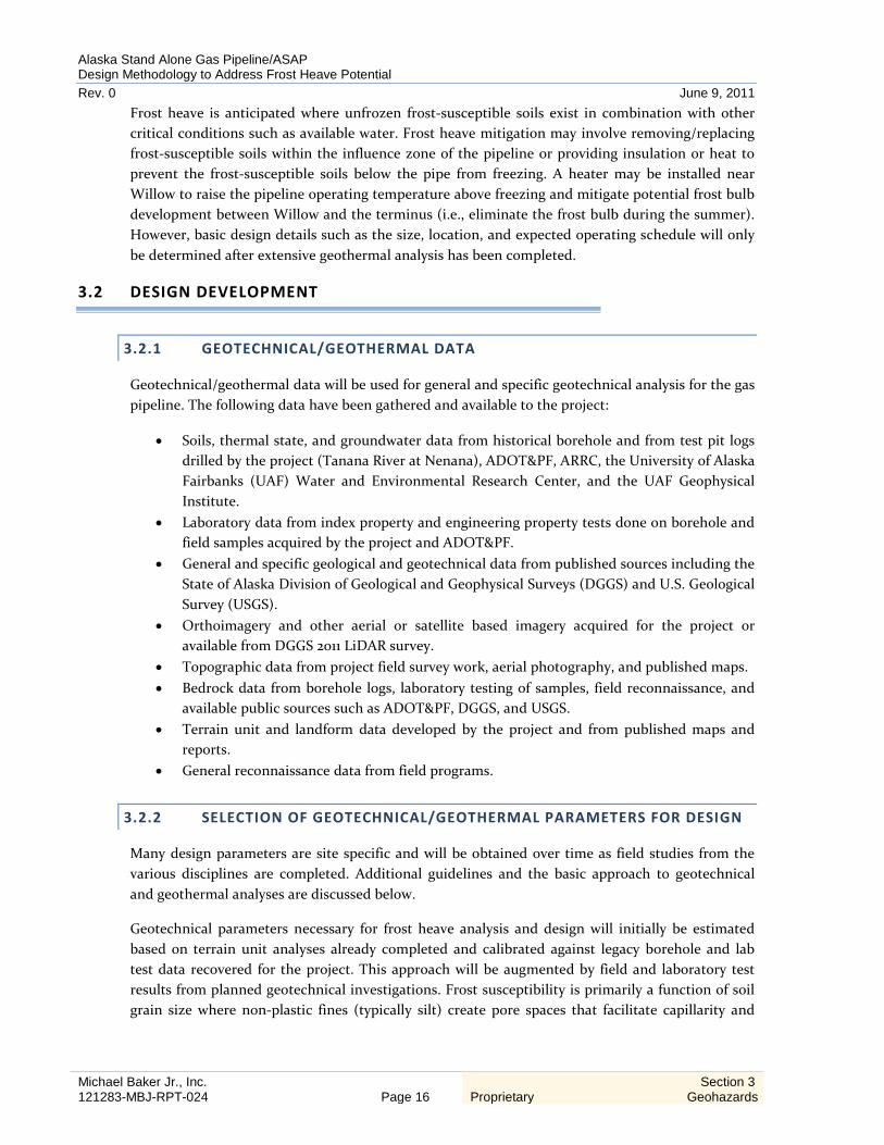
Frost heave is anticipated where unfrozen frost-susceptible soils exist in combination with other critical conditions such as available water. Frost heave mitigation may involve removing/replacing frost-susceptible soils within the influence zone of the pipeline or providing insulation or heat to prevent the frost-susceptible soils below the pipe from freezing. A heater may be installed near Willow to raise the pipeline operating temperature above freezing and mitigate potential frost bulb development between Willow and the terminus (i.e., eliminate the frost bulb during the summer). However, basic design details such as the size, location, and expected operating schedule will only be determined after extensive geothermal analysis has been completed.
3.2 DESIGN DEVELOPMENT
3.2.1 GEOTECHNICAL/GEOTHERMAL DATA
Geotechnical/geothermal data will be used for general and specific geotechnical analysis for the gas pipeline. The following data have been gathered and available to the project:
• Soils, thermal state, and groundwater data from historical borehole and from test pit logs drilled by the project (Tanana River at Nenana), ADOT&PF, ARRC, the University of Alaska Fairbanks (UAF) Water and Environmental Research Center, and the UAF Geophysical Institute.
• Laboratory data from index property and engineering property tests done on borehole and field samples acquired by the project and ADOT&PF.
• General and specific geological and geotechnical data from published sources including the State of Alaska Division of Geological and Geophysical Surveys (DGGS) and U.S. Geological Survey (USGS).
• Orthoimagery and other aerial or satellite based imagery acquired for the project or available from DGGS 2011 LiDAR survey.
• Topographic data from project field survey work, aerial photography, and published maps. • Bedrock data from borehole logs, laboratory testing of samples, field reconnaissance, and
available public sources such as ADOT&PF, DGGS, and USGS. • Terrain unit and landform data developed by the project and from published maps and
reports. • General reconnaissance data from field programs.
3.2.2 SELECTION OF GEOTECHNICAL/GEOTHERMAL PARAMETERS FOR DESIGN
Many design parameters are site specific and will be obtained over time as field studies from the various disciplines are completed. Additional guidelines and the basic approach to geotechnical and geothermal analyses are discussed below.
Geotechnical parameters necessary for frost heave analysis and design will initially be estimated based on terrain unit analyses already completed and calibrated against legacy borehole and lab test data recovered for the project. This approach will be augmented by field and laboratory test results from planned geotechnical investigations. Frost susceptibility is primarily a function of soil grain size where non-plastic fines (typically silt) create pore spaces that facilitate capillarity and

Alaska Stand Alone Gas Pipeline/ASAP Design Methodology to Address Frost Heave Potential Rev. 0 June 9, 2011
Michael Baker Jr., Inc. 121283-MBJ-RPT-024 Page 17
Section 3 Proprietary Geohazards
freezing point depression. The U.S. Army Corps of Engineers frost design and classification system is a universal standard for addressing frost heave behavior (see Table 3.1). Critical conditions for pipeline frost heave distress occur where the pipeline traverses abrupt contrasts in soil conditions and the soils freeze and thaw repeatedly (seasonally).
Note that the frost classification system is based primarily on soil particle size distribution. Geotechnical tests to properly classify and analyze frost heave potential include the following tests with corresponding standard test methods.
Table 3.1 U.S. Army Corps of Engineers Frost Design Soil Classification System
Frost Susceptibilitya Frost Group Note Kind of soil
Amount finer than 0.02mm
(wt%) Typical soil type under USCSb
Negligible to low NFSc a Gravels 0 to 1.5 GW, GP
b Sands 0 to 3 SW, SP
Possible PFSd a Gravels 1.5 to 3 GW, GP
b Sands 3 to 10 SW, SP
Low to medium S1 Gravels 3 to 6 GW, GP, GW-GM, GP-GM
Very low to high S2 Sands 3 to 6 SW, SP, SW-SM, SP-SM
Very low to high F1 Gravels 6 to 10 GM, GW-GM, GP-GM
Medium to high F2 a Gravels 10 to 20 GM, GM-GC, GW-GM, GP-GM
Very low to very high b Sands 6 to 15 SM, SW-SM, SP-SM
Medium to high F3 a Gravels >20 GM, GC
Low to high b Sands except very fine silty sands
>15 SM, SC
Very low to very high c Clays, Ip>12 - CL,CH
Low to very high F4 a All silts - ML, MH
Very low to high b Very fine silty sands >15 SM
Low to very high c Clays, Ip>12 - CL, CL-ML
Very low to very high d Varved clays and other fine-grained banded sediments
- CL and ML; CL, ML, and SM; CL, CH, and ML; CL, CH, ML, and SM
a Based on laboratory frost-heave tests b G, gravel; S, sand; M, silt; W, well graded; P, poorly graded; H, high plasticity; L, low plasticity c Non-frost susceptible d Requires laboratory frost-heave test to determine frost susceptibility Source: Johnson et. al. 1986
(Andersland and Ladanyi 2004)

Alaska Stand Alone Gas Pipeline/ASAP Design Methodology to Address Frost Heave Potential Rev. 0 June 9, 2011
Michael Baker Jr., Inc. 121283-MBJ-RPT-024 Page 18
Section 3 Proprietary Geohazards
Table 3.2 Geotechnical Tests for Frost Heave Potential
Test Standard
Moisture content ASTM D2216
Gradation (sieve analysis) ASTM C136
Gradation (sieve with hydrometer) ASTM D422
Atterberg Limits ASTM D4318
Table 3.3 Additional Geotechnical Tests for Frost Heave Evaluation
Test Standard
Moisture-Density Relationship ASTM D1557
Specific Gravity ASTM C127
Unit Weight of Frozen Soil Gravimetric test of undisturbed frozen soil
Additional geotechnical parameters needed to forecast frost heave include permeability, pressure on the freezing front; frost penetration rate and frost heaving rate; longitudinal, bearing and uplift resistance; soil load/deflection and creep characteristics; soil temperature gradient, and climatic data. Many of these parameters can be empirically correlated with the results of geotechnical tests listed above. A probabilistic approach to assigning soil properties may be adopted if sufficient sample data is acquired by the project. When data gaps are identified, they will be filled as necessary. Climatic data will be updated to include most recent data from stations along the route. Limits of applicability of climatic data will be based on geographic similarities along the line.
The approach to frost heave analysis will be to combine route soils data with climatic data and pipeline thermal predictions and pipe deformation analysis. Thermal conditions of the pipeline and ground will be predicted using a coupled hydraulics/geothermal model. This model will be comprised of a linear hydraulics model of the pipeline with two-dimensional “slices” of soil defined at intervals along the pipeline. The slices are defined principally by the terrain unit analysis, thus geotechnical information will accompany each slice that allows prediction of frost heave. The hydraulics model will predict temperatures along the pipeline for a given throughput, inlet temperature and pressure, initial soil temperatures, and gas properties. The pressure and temperature of the flowing gas depends upon the heat flux through the pipe wall which, in turn, depends on the pipe interaction with the subsurface thermal state (ground temperatures).
Predictions of the ground temperatures surrounding the pipe will be made by the geothermal model. The model will consider a two-dimensional “slice” of the pipe surrounded by soil regions and bounded on the surface by location dependent varying climatic functions. A finite element
Alaska Stand Alone Gas Pipeline/ASAP Design Methodology to Address Frost Heave Potential Rev. 0 June 9, 2011
Michael Baker Jr., Inc. 121283-MBJ-RPT-024 Page 19
Section 3 Proprietary Geohazards
approach will be applied to develop a series of “snapshots” along the pipeline of the changing thermal condition of the subsurface over time, which is in turn used to estimate the heat flux along the alignment to the flowing gas. The result is an estimate of the magnitude and timing of freezing of initially thawed ground including the geometry of the evolving frost bulb. The same process is used to predict thawing of initially frozen ground.
The pipe/soil thermal regime and geotechnical properties that define the soil’s frost susceptibility will then be used to predict the amount of heave beneath the pipeline. The frost heave predictions will be calibrated against results of previous frost heave laboratory and field testing performed by the research community and special testing completed by industry for other projects.
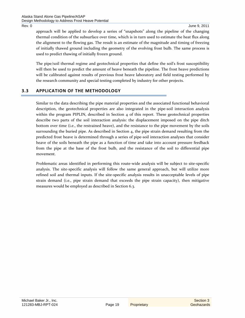
3.3 APPLICATION OF THE METHODOLOGY
Similar to the data describing the pipe material properties and the associated functional behavioral description, the geotechnical properties are also integrated in the pipe-soil interaction analysis within the program PIPLIN, described in Section 4 of this report. These geotechnical properties describe two parts of the soil interaction analysis: the displacement imposed on the pipe ditch bottom over time (i.e., the restrained heave), and the resistance to the pipe movement by the soils surrounding the buried pipe. As described in Section 4, the pipe strain demand resulting from the predicted frost heave is determined through a series of pipe-soil interaction analyses that consider heave of the soils beneath the pipe as a function of time and take into account pressure feedback from the pipe at the base of the frost bulb, and the resistance of the soil to differential pipe movement.
Problematic areas identified in performing this route-wide analysis will be subject to site-specific analysis. The site-specific analysis will follow the same general approach, but will utilize more refined soil and thermal inputs. If the site-specific analysis results in unacceptable levels of pipe strain demand (i.e., pipe strain demand that exceeds the pipe strain capacity), then mitigative measures would be employed as described in Section 6.3.

Alaska Stand Alone Gas Pipeline/ASAP Design Methodology to Address Frost Heave Potential Rev. 0 June 9, 2011
Michael Baker Jr., Inc. 121283-MBJ-RPT-024 Page 20
Section 4 Proprietary Strain Demand Determination
SECTION 4. STRAIN DEMAND DETERMINATION
4.1 PIPE-SOIL INTERACTION ANALYSIS OVERVIEW
The mechanism of pipeline frost heave has been investigated in detail for many previous arctic gas pipeline projects. Frost heave occurs when a chilled pipeline freezes water in frost-susceptible soil in which it is buried. As the soil freezes, it expands and forms a frost bulb around the pipe. Upward heave of the pipe is produced by swelling at the bulb face as the bulb grows. Significant pipe stresses and deformations can occur when the buried pipeline runs between a stable soil and a frost-susceptible soil. Because the pipe heaves in the frost-susceptible soil section but remains stationary in the adjacent stable soil section, a differential vertical heave displacement profile is produced across the transition between the stable and frost-susceptible soil sections.
The strain demand analyses for frost heave of ASAP will be carried out using the PIPLIN computer program (SSD 2011). PIPLIN is a special-purpose finite element program developed to perform stress and deformation analysis of two-dimensional pipeline configurations. The analyses will consider several nonlinear aspects of pipeline behavior, including pipe yield, large-displacement effects, and nonlinear frozen soil support.
A heaving section of a pipeline together with a schematic view of the corresponding PIPLIN model is illustrated in Figure 4.1. To reduce the required size of the model, a symmetric boundary condition (i.e., zero rotation and zero longitudinal translation) is normally imposed at the end of the model corresponding to the center of the heave span. The sufficient model length is such that the boundary condition specified at the remote end of the model has no influence on the key analysis results. The pipe is typically assumed to be initially straight with a uniform depth of soil cover.
The pipe is modeled using beam type elements in which the stresses and strains are monitored at a number of fiber points around the pipe cross section at the element ends. PIPLIN achieves additional economy by considering a plane of symmetry through the pipe centerline (e.g., the vertical plane in frost heave model) so that only one-half of the pipe cross section is analyzed. In these analyses, the pipe cross-section is assumed to remain circular and plane sections are assumed to remain plane. The pipe element accounts for large displacement effects (i.e., changes in the equilibrium due to large displacements) by adding geometric stiffness coefficients to the element stiffness matrix. This allows PIPLIN models to accurately capture important column buckling and cable tension effects.

Alaska Stand Alone Gas Pipeline/ASAP Design Methodology to Address Frost Heave Potential Rev. 0 June 9, 2011
Michael Baker Jr., Inc. 121283-MBJ-RPT-024 Page 21
Section 4 Proprietary Strain Demand Determination
Figure 4.1 Frost Heave Illustration
Pipe yield at the fiber points around the pipe cross section is taken into account assuming the von Mises yield criterion so that interaction between hoop and longitudinal stresses is included. The pipe steel material is modeled using the Mroz (Mroz 1967) multi-linear kinematic hardening plasticity model which is able to accurately capture anisotropic pipe steel stress-strain relationships
Heave Span
Frozen Boundary SectionProvides Strong Frozen
Resistance to Pipe Movement
Frozen Boundary SectionProvides Strong Frozen
Resistance to Pipe Movement
Initially Unfrozen Central SectionGrows a Frost Bulb Over Time Bulb
Growth Causes Differential Frost Heave
BuriedChilledPipeline
To Virtual Anchor Pipeline Modeled Using Inelastic Pipe Elementswith Geometric StiffnessSymmetric Boundary Condition at Mid-Span
Loading Sequence:GravityInternal PressureTemperature DifferentialHeave
Soil Modeled as Nonlinear Winkler Foundation
Center of Symmetry

Alaska Stand Alone Gas Pipeline/ASAP Design Methodology to Address Frost Heave Potential Rev. 0 June 9, 2011
Michael Baker Jr., Inc. 121283-MBJ-RPT-024 Page 22
Section 4 Proprietary Strain Demand Determination
(e.g., pipe that has different stress-strain curves in the longitudinal tension/compression vs. hoop tension/compression directions). The pipe material model provides a very reasonable representation of steel behavior under monotonic, unloading and cyclic load conditions.
The soil is modeled as a nonlinear Winkler foundation. This means that the soil support is idealized as a series of discrete, independent, nonlinear springs lumped at the element midpoints. In effect, this assumes that the soil can be regarded as a series of plane “slices”. The basic assumption is that the slices deform independently of each other. The pipe-soil springs are assumed to have uniform properties over any pipe segment.
The frost heave analyses are typically initiated with the application of gravity, internal pressure and temperature differential loads. If desired, a hydrostatic test loading/unloading sequence can be considered prior to applying the operating loads. A multi-year (typically 20 to 30 years) frost heave simulation of the pipe-soil interaction model is then undertaken. The frost heave analyses are nonlinear time-history analyses performed using small steps through time. Within the heave span, the frost bulb geometry and frost heave vary with time. Seasonal variations of the uplift, longitudinal, and bearing creep soil temperatures (and corresponding resistance) are also specified with each heave time step. The heave is imposed progressively at the base of the pipe-soil springs within the heave span. The amount of heave at the ditch bottom is calculated separately for each transverse pipe-soil support in turn accounting for the important pressure feedback from the pipe at the base of the frost bulb. A transition length between the finite length section of heaving soil and the adjacent non-heaving soil section can be specified if desired.
The complete pipe-soil deformation state is established at each increment of the analysis. The program output includes pipe displacements, soil support deformations and reactions; pipe axial forces, bending moments and curvatures; axial, hoop and von Mises stresses and axial and hoop strains in the pipe. The maximum pipe tension and compression strain demands are established at each output state to provide time-history plots of these key response quantities.
4.2 PIPE MATERIAL PROPERTIES
As implemented in PIPLIN, the Mroz plasticity model assumes that the pipe material yields according to the von Mises theory under plane-stress conditions. The bi-axial stress-strain behavior is defined by a set of progressively larger, non-overlapping elliptical yield surfaces in longitudinal stress vs. hoop stress space. The Mroz theory specifies that as the steel yields, the individual ellipses translate without changing size or shape, which is the well-known kinematic hardening assumption. The theory also specifies the direction of movement of each ellipse – essentially, any ellipse moves so that when the stress point reaches the next larger ellipse, the yielding ellipses do not overlap.
One of the key features of the PIPLIN steel model is that the elliptical yield functions can be shifted to initial positions in order to mimic the effects of the pipe expansion phase of the UOE manufacturing process. The shifts are selected such that the analytical uniaxial stress-strain results closely match a set of uniaxial longitudinal tension (LT), hoop tension (HT) target stress-strain curves. For pipe steel fabricated with the UOE process, the ellipses tend to be shifted along the HT axis. The pure HT ellipse shifting pattern tends to result in an elevated proportional limit and

Alaska Stand Alone Gas Pipeline/ASAP Design Methodology to Address Frost Heave Potential Rev. 0 June 9, 2011
Michael Baker Jr., Inc. 121283-MBJ-RPT-024 Page 23
Section 4 Proprietary Strain Demand Determination
relatively sharp (abrupt) yielding point for the HT curve (due to work hardening and bunching of the ellipses) and a low proportional limit with progressive (well rounded) yielding for the hoop compression (HC) curve (due to Bauschinger effect). The steel model is well suited for capturing key aspects of the anisotropy patterns typically observed in UOE pipe.
As described in “A Material Model for Pipeline Steels” (Hart, et. al 1996), an 8-parameter model can be used to develop input material properties for strain levels below 2%. This portion of the steel stress-strain curve can be divided into 3 regions namely; a linear elastic region, a curved transition or “knee” region, and an essentially linear “fully plastic” region. The term “fully plastic” is not strictly correct since the steel still has a finite hardening modulus. The model requires that the HT and LT curves have the same elastic modulus and the same fully-plastic strain hardening modulus. However, the shape of the HT and LT curves in the yield transition region can be different i.e., the curves can have different proportional limits and different degrees of “sharpness” or “roundedness” through the transition from elastic to fully-plastic conditions. The strength levels of the curves in the fully-plastic strain hardening region need not be the same. A 2-root fitting process can be used to determine the ellipse sizes and initial shifts required to closely match a given “target” LT-HT pair of stress-strain curves (as well as a 3-root fitting process when a “target” LT-HT-LC triple of stress-strain curves is available).
4.3 GEOTHERMAL INPUT
Frost heave is associated with growth of a frost bulb around the chilled pipe and it is assumed that heave is produced by swelling at the bulb face as the frost bulb grows wider and deeper (see Figure 4.2). The amount of heave for a given increase in frost bulb depth is influenced by several parameters including the type of soil, the availability of moisture, the speed with which the frost bulb grows, the bearing pressure exerted by the pipe on the ditch bottom and other factors. In addition, the amount of movement at the ditch bottom depends on the depth of the frost bulb, with a given amount of swelling producing less ditch bottom heave as the frost bulb gets progressively deeper. Free heave is the heave that would occur if the pipeline provided no resistance to movement. Restrained heave, which is less than the free heave, is the heave that results accounting for the pipelines resistance to movement which tends to increases the amount of pressure at the base of the frost bulb.

Alaska Stand Alone Gas Pipeline/ASAP Design Methodology to Address Frost Heave Potential Rev. 0 June 9, 2011
Michael Baker Jr., Inc. 121283-MBJ-RPT-024 Page 24
Section 4 Proprietary Strain Demand Determination
Figure 4.2 Frost Bulb Schematic
PIPLIN analyzes the effects of restrained frost heave by treating heave movements as equivalent support "settlements," applied at the ditch bottom (i.e., at the base of the bearing springs). Because heave originates at the frost bulb face, a theory is needed to convert swelling of the soil into ditch bottom movements. PIPLIN has several different options for specifying pipeline frost heave effects. The “Revised Formula Method” is the option selected for the ASAP project. In the Revised Formula Method, the program calculates ditch bottom movements using the segregation potential theory (Konrad 1981) given certain information describing the frost bulb properties.
The following time-independent parameters are specified:
(1) A reference pressure “Po” to be used in the segregation potential equation. (2) The frost bulb density “γ” which is used to calculate the soil pressure at the frost bulb base
due to bulb self weight. (3) The equivalent burial depth “Do” which is used in the calculation of soil pressure. (4) The initial overburden force correction term “Fo” which is used in the calculation of soil
pressure.
In addition to the time-independent parameters described above, time-histories of the following frost bulb and soil properties are provided as an input table:
(1) Frost bulb depth “D” below pipe. (2) Shear force per foot of pipe “S”. In general, the shear force term can be due to side shear
and/or end shear effects. Note that because a time-history of S is input, seasonal variations can be directly included.
(3) Bearing width “BS” at the base of the frost bulb over which the shear force S is assumed to be distributed. That is, the soil bearing pressure at the frost bulb base due to S is S/BS.
Frost Bulb Width
Frost Bulb Depth
Chilled Buried Pipeline
Frost Bulb

Alaska Stand Alone Gas Pipeline/ASAP Design Methodology to Address Frost Heave Potential Rev. 0 June 9, 2011
Michael Baker Jr., Inc. 121283-MBJ-RPT-024 Page 25
Section 4 Proprietary Strain Demand Determination
(4) Bearing width, BF, at the base of the frost bulb over which the ditch bottom bearing force, F, is assumed to be distributed. The soil bearing pressure at the frost bulb base due to F is F/BF.
(5) Temperature gradient “G”, at the frost front. (6) The coefficient “a” to be used in the segregation potential equation. (7) A reference segregation potential “SPo” at the reference pressure “Po”.
At any given time “t” and at any given point within the heaving section of the pipe, the values of D(t), S(t), BS(t), BF(t), G(t), a(t) and SPo(t) can be obtained from the input time-history table. Note that for most applications, the values of a and SPo are constant with time. One exception to this is for a layered soil profile where a and SPo may vary with depth. The variation with depth can be considered indirectly as a variation with the times that the bottom of frost bulb reaches the different soil layers. When a pipe segment has a different heave material at each end (e.g., when considering a heave material transition), the heave material properties at a given transverse support location are obtained by linear interpolation between the properties at end “I” and end “J” of the segment. The values of S, D, BS, BF and G are calculated at the middle of the time step, by interpolation in the input time-histories. The pressure to be used in the equation for heave rate is computed as follows:
FS BFF
BSDDP )( + + )+ ( = 0
0−γ
where the parameters γ, D, Do, S, BS, Fo and BF are defined above. The term “F” is the feedback force exerted by the pipe on the ditch bottom per unit length of pipe (i.e., F is equal to the current transverse (T) support reaction). As already noted, the quantities γ, Do and Fo are constants and the quantities D, S, BS and BF vary with time. The bearing force F is obtained from analysis of the interaction between the pipe and soil, and varies with location along the pipe as well as with time. If overburden (soil plus pipe) loads are specified, the initial pipe bearing force will equal the overburden soil weight plus the pipe weight. The initial value of the pressure for heave calculations will thus include the effect of the soil weight at the ditch bottom level (in the γ D0 pressure term) plus the effect of the overburden soil weight (in the (F-Fo)/BF pressure term). If no Fo correction is made, the overburden soil weight will be included in the pressure calculation twice. The parameters Do and Fo are selected to provide the desired initial pressure for heave calculations. The shear resistance term S can be used to represent the resistance provided by the unfrozen soil on the sides of the soil “block” above the widest point of the frost bulb and/or the resistance provided by the frozen soil “abutments” at each end of the heaving span.
When the frost bulb depth increases during an analysis time step, the heave rate, )(tH , is
calculated using the segregation potential equation:
)()(09.1)( ))()((0
0 tGetSPtH PtPta −=
and the heave increment is given by:
)( ttHH ∆=∆
Alaska Stand Alone Gas Pipeline/ASAP Design Methodology to Address Frost Heave Potential Rev. 0 June 9, 2011
Michael Baker Jr., Inc. 121283-MBJ-RPT-024 Page 26
Section 4 Proprietary Strain Demand Determination
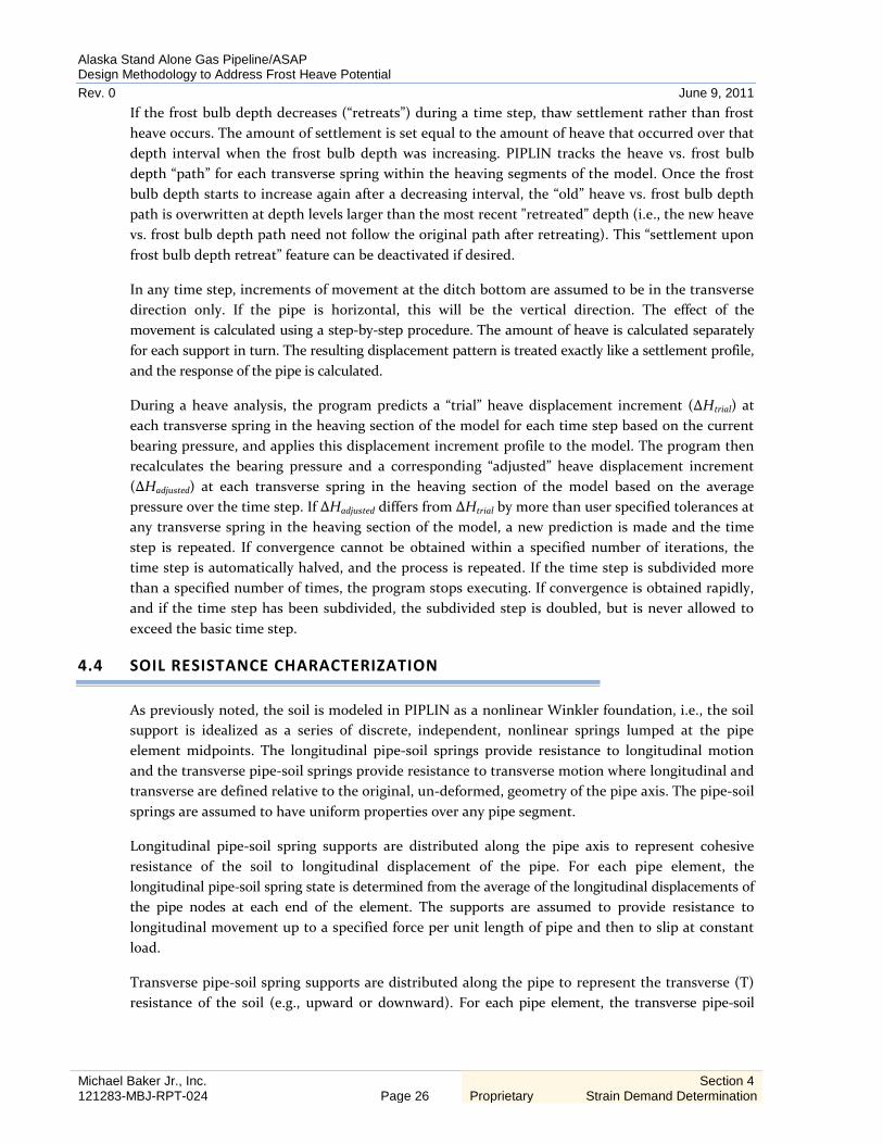
If the frost bulb depth decreases (“retreats”) during a time step, thaw settlement rather than frost heave occurs. The amount of settlement is set equal to the amount of heave that occurred over that depth interval when the frost bulb depth was increasing. PIPLIN tracks the heave vs. frost bulb depth “path” for each transverse spring within the heaving segments of the model. Once the frost bulb depth starts to increase again after a decreasing interval, the “old” heave vs. frost bulb depth path is overwritten at depth levels larger than the most recent "retreated” depth (i.e., the new heave vs. frost bulb depth path need not follow the original path after retreating). This “settlement upon frost bulb depth retreat” feature can be deactivated if desired.
In any time step, increments of movement at the ditch bottom are assumed to be in the transverse direction only. If the pipe is horizontal, this will be the vertical direction. The effect of the movement is calculated using a step-by-step procedure. The amount of heave is calculated separately for each support in turn. The resulting displacement pattern is treated exactly like a settlement profile, and the response of the pipe is calculated.
During a heave analysis, the program predicts a “trial” heave displacement increment (∆Htrial) at each transverse spring in the heaving section of the model for each time step based on the current bearing pressure, and applies this displacement increment profile to the model. The program then recalculates the bearing pressure and a corresponding “adjusted” heave displacement increment (∆Hadjusted) at each transverse spring in the heaving section of the model based on the average pressure over the time step. If ∆Hadjusted differs from ∆Htrial by more than user specified tolerances at any transverse spring in the heaving section of the model, a new prediction is made and the time step is repeated. If convergence cannot be obtained within a specified number of iterations, the time step is automatically halved, and the process is repeated. If the time step is subdivided more than a specified number of times, the program stops executing. If convergence is obtained rapidly, and if the time step has been subdivided, the subdivided step is doubled, but is never allowed to exceed the basic time step.
4.4 SOIL RESISTANCE CHARACTERIZATION
As previously noted, the soil is modeled in PIPLIN as a nonlinear Winkler foundation, i.e., the soil support is idealized as a series of discrete, independent, nonlinear springs lumped at the pipe element midpoints. The longitudinal pipe-soil springs provide resistance to longitudinal motion and the transverse pipe-soil springs provide resistance to transverse motion where longitudinal and transverse are defined relative to the original, un-deformed, geometry of the pipe axis. The pipe-soil springs are assumed to have uniform properties over any pipe segment.
Longitudinal pipe-soil spring supports are distributed along the pipe axis to represent cohesive resistance of the soil to longitudinal displacement of the pipe. For each pipe element, the longitudinal pipe-soil spring state is determined from the average of the longitudinal displacements of the pipe nodes at each end of the element. The supports are assumed to provide resistance to longitudinal movement up to a specified force per unit length of pipe and then to slip at constant load.
Transverse pipe-soil spring supports are distributed along the pipe to represent the transverse (T) resistance of the soil (e.g., upward or downward). For each pipe element, the transverse pipe-soil
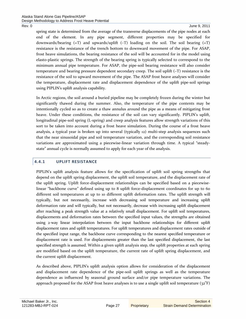
Alaska Stand Alone Gas Pipeline/ASAP Design Methodology to Address Frost Heave Potential Rev. 0 June 9, 2011
Michael Baker Jr., Inc. 121283-MBJ-RPT-024 Page 27
Section 4 Proprietary Strain Demand Determination
spring state is determined from the average of the transverse displacements of the pipe nodes at each end of the element. In any pipe segment, different properties may be specified for downwards/bearing (+T) and upwards/uplift (–T) loading on the soil. The soil bearing (+T) resistance is the resistance of the trench bottom to downward movement of the pipe. For ASAP, frost heave simulations, the bearing resistance of the soil will be accounted for in the model using elasto-plastic springs. The strength of the bearing spring is typically selected to correspond to the minimum annual pipe temperature. For ASAP, the pipe-soil bearing resistance will also consider temperature and bearing pressure dependent secondary creep. The soil uplift (–T) resistance is the resistance of the soil to upward movement of the pipe. The ASAP frost heave analyses will consider the temperature, displacement rate and displacement dependence of the uplift pipe-soil springs using PIPLIN’s uplift analysis capability.
In Arctic regions, the soil around a buried pipeline may be completely frozen during the winter but significantly thawed during the summer. Also, the temperature of the pipe contents may be intentionally cycled so as to create a thaw annulus around the pipe as a means of mitigating frost heave. Under these conditions, the resistance of the soil can vary significantly. PIPLIN’s uplift, longitudinal pipe-soil spring (L-spring) and creep analysis features allow strength variations of this sort to be taken into account during a frost heave simulation. During the course of a frost heave analysis, a typical year is broken up into several (typically 12) multi-step analysis sequences such that the near sinusoidal pipe and soil temperature variation, and the corresponding soil resistance variations are approximated using a piecewise-linear variation through time. A typical “steady-state” annual cycle is normally assumed to apply for each year of the analysis.
4.4.1 UPLIFT RESISTANCE
PIPLIN’s uplift analysis feature allows for the specification of uplift soil spring strengths that depend on the uplift spring displacement, the uplift soil temperature, and the displacement rate of the uplift spring. Uplift force-displacement relationships can be specified based on a piecewise-linear “backbone curve” defined using up to 8 uplift force-displacement coordinates for up to 60 different soil temperatures at up to 10 different uplift deformation rates. The uplift strength will typically, but not necessarily, increase with decreasing soil temperature and increasing uplift deformation rate and will typically, but not necessarily, decrease with increasing uplift displacement after reaching a peak strength value at a relatively small displacement. For uplift soil temperatures, displacements and deformation rates between the specified input values, the strengths are obtained using 2-way linear interpolation between the input backbone relationships for different uplift displacement rates and uplift temperatures. For uplift temperatures and displacement rates outside of the specified input range, the backbone curve corresponding to the nearest specified temperature or displacement rate is used. For displacements greater than the last specified displacement, the last specified strength is assumed. Within a given uplift analysis step, the uplift properties at each spring are modified based on the uplift temperature, the current rate of uplift spring displacement, and the current uplift displacement.
As described above, PIPLIN’s uplift analysis option allows for consideration of the displacement and displacement rate dependence of the pipe-soil uplift springs as well as the temperature dependence as influenced by seasonal ground surface and/or pipe temperature variations. The approach proposed for the ASAP frost heave analyses is to use a single uplift soil temperature (32oF)

Alaska Stand Alone Gas Pipeline/ASAP Design Methodology to Address Frost Heave Potential Rev. 0 June 9, 2011
Michael Baker Jr., Inc. 121283-MBJ-RPT-024 Page 28
Section 4 Proprietary Strain Demand Determination
corresponding to thawed soil conditions together with two or more uplift soil temperatures to cover the range of frozen soil temperature conditions encountered over a typical year of operation during the frost heave analysis. The uplift temperature values and the time between adjacent temperature values are specified for a typical 1 year analysis cycle. The uplift soil temperature will be taken as equal to the pipe temperature or some measure of the average backfill temperature, both of which have a seasonal variation that resembles a sine wave. The ASAP project proposes to compute the thawed and frozen uplift pipe-soil spring properties based on publically available geotechnical procedures (e.g., see COLTKBR 2003 and COLTKBR 2007).
4.4.2 BEARING RESISTANCE
PIPLIN has sophisticated creep support analysis capabilities including pressure and temperature dependent primary and secondary creep. If desired, creep properties can be associated with any transverse segment support, and creep analyses can be carried out. The pressure and temperature dependence is considered by specifying the creep parameters at up to 5 temperatures for up to 20 pressures. For temperatures and pressures within the specified temperature and pressure ranges, the creep parameters are obtained by linear interpolation between input values. For temperatures and pressures that are outside of the specified temperature and pressure ranges, the creep parameters associated with the nearest input temperature or pressure are used.
For the ASAP frost heave analyses, it is proposed to consider secondary creep in the bearing pipe-soil supports. Including secondary creep has the effect of adding a secondary creep dashpot – a viscous support element that provides resistance proportional to the velocity – (with a dashpot coefficient Cs) in series with the elastic-perfectly plastic bearing spring associated with each pipe element. The dashpot coefficient Cs is specified to be dependent on both temperature and the bearing pressure between the pipe and soil, typically decreasing with increasing temperature and pressure. The ASAP project proposes to use publically available geotechnical procedures (COLTKBR 2007) to compute the bearing spring and dashpot properties.
4.4.3 LONGITUDINAL RESISTANCE
In any segment, the strength of the L-spring can be defined to vary with temperature, by specifying up to 20 temperatures and up to 20 corresponding strengths. For temperatures between the specified values, the strengths are obtained by linear interpolation. For temperatures outside of the specified range, the strength corresponding to the nearest specified temperature is assumed. An initial temperature (the same for all segments) is specified, and this determines the L-spring strength at the beginning of the analysis. The effect is to place an upper limit on the strength of the L-spring. If this strength is exceeded at any location, the stiffness is reduced to zero. The effect, initially, is exactly as if a stiffness (K) value of zero had been specified for the support. However, the behavior differs from that with K=0, because the strength can subsequently be changed.
In any load sequence, it can be specified that the longitudinal (L-spring) soil temperature changes progressively, so that the cutoff on the strength also changes. If the strength decreases, the resistance developed by the support is progressively reduced, leading to a redistribution of load along the pipeline. If the strength increases, the support force remains unchanged but the stiffness becomes nonzero (the value on the basic force-displacement relationship for the current support

Alaska Stand Alone Gas Pipeline/ASAP Design Methodology to Address Frost Heave Potential Rev. 0 June 9, 2011
Michael Baker Jr., Inc. 121283-MBJ-RPT-024 Page 29
Section 4 Proprietary Strain Demand Determination
force). In this case there is no redistribution of load. The strength may be cycled in any desired way, for as many seasonal cycles as desired.
As described above, L-spring analysis allows for consideration of the temperature dependence of the pipe-soil longitudinal springs as influenced by seasonal surface and/or pipe temperature variations. The approach proposed for the ASAP frost heave analysis is to specify a single longitudinal soil temperature corresponding to thawed soil conditions together with several additional longitudinal soil temperatures to cover the range of frozen soil temperature conditions encountered over a typical year of operation during the frost heave analysis. The longitudinal temperature values and the time between adjacent temperature values are specified for a typical one year analysis cycle. The longitudinal soil temperature will be taken as equal to the pipe temperature which has a seasonal variation that resembles a sine wave. For ASAP, the thawed longitudinal pipe-soil spring properties will be computed using conventional procedures (e.g., see ASCE 1984, Hart et. al 2001, and Honegger et. al 2004). For frozen soil conditions, the ASAP project proposes to utilize publically available geotechnical procedures (COLTKBR 2007) for estimating the pipe-soil longitudinal spring relationship.
4.5 MODEL GEOMETRY
The typical model geometry consists of a straight, horizontal section of the pipeline with a uniform depth of frozen soil cover. The chilled pipeline is assumed to cross an initially thawed span – this is the location where a frost bulb will grow around the pipe resulting in differential frost heave. A plane of symmetry is assumed at the center of the heaving span so that only one-half of the heaving pipeline configuration is analyzed. A transition length (or ramp) between the finite length section of heaving soil and the adjacent non-heaving soil section can be specified if desired. A multi-span analysis approach is undertaken considering different simulations for on the order of 10 different span lengths ranging from very short spans (e.g., down to say 10 feet) to very long spans (e.g., up to say 150 feet). The variation in span length is an important consideration because shorter spans, which are often associated with relatively high levels of strain per inch of heave tend to be “shut down” due to pressure feedback effects (i.e., high bearing pressures increase the stresses at the base of the frost bulb which tends to shut down frost heave). For very long spans, the imposed heave profile approaches a step-change (e.g., similar to a fault crossing). The end result of the multi-span evaluation approach is that it leads to a “critical span” corresponding to the span with the highest strain demand at a given point in time. The critical span length depends on several parameters including the pipe stiffness, the soil resistance and the pressure sensitivity of the heaving soil.
4.6 IMPOSED LOADS
As previously mentioned, frost heave analyses are typically initiated with the application of gravity, internal pressure and temperature differential loads. If desired, a hydrostatic test loading and unloading sequence can be included prior to applying the operating loads. A multi-year frost heave evaluation of the pipe-soil interaction model is then undertaken holding the gravity and internal pressure loads constant. The applied temperature differential can be varied in a sinusoidal pattern over each year of the simulation based on the difference between the time-varying pipe temperature and the constant tie-in temperature. The frost heave analyses are nonlinear time-

Alaska Stand Alone Gas Pipeline/ASAP Design Methodology to Address Frost Heave Potential Rev. 0 June 9, 2011
Michael Baker Jr., Inc. 121283-MBJ-RPT-024 Page 30
Section 4 Proprietary Strain Demand Determination
history analyses performed using small steps through time. Within the heave span, the frost bulb geometry and frost heave vary with time. Seasonal variations of the uplift, longitudinal and creep soil temperatures are specified with each heave time step. The heave is imposed progressively at the base of the pipe-soil springs within the heave span. The amount of heave at the ditch bottom is calculated separately for each transverse pipe-soil support in turn accounting for pressure feedback.
For a selected heave span length, the results from a PIPLIN frost heave analysis include a detailed output of the state of the pipe-soil interaction model at each time step. The output state includes the current time, the pipe axial force, bending moment, hoop stress, top and bottom fiber von Mises stress, longitudinal stress, hoop strain and longitudinal strain and the curvature at each node of the pipeline model. The output state also includes the uplift, creep and longitudinal soil control temperatures, the longitudinal and transverse spring forces and displacements, the uplift spring displacement rate and the creep displacements for each element of the pipeline model. At the pipe-soil spring locations within the heaving section of the model, the frost bulb width, depth and shear are available together with the pressure components at the base of the frost bulb due to the frost bulb weight, the transverse pipe-soil spring, and shear as well as the total pressure. The current unrestrained mid-span free heave is also provided. The results described above can be post-processed in a number of different ways. Spatial plots and time history plots of various response quantities usually provide the most useful methods for understanding and interpreting the results. It is also possible to develop animations of various spatial response plots to gain a better understanding of how the overall results vary over the course of the multi-year analysis duration.
The most important results from a frost heave simulation for a given span length are the time histories of the maximum tension and compression strain demands. Detailed processing of the PIPLIN deflected shape at each point in time is used to develop time history plots of “digitally pigged” bending strains or curvatures which provides a basis for relating geometry monitoring data (e.g., smart pig survey data) to the corresponding nodal tension and compression strain demands. A schematic illustration of the maximum pig curvature is presented in Figure 4.3 for a 25-year frost heave simulation. Note that the “wiggles” in the curvature time history plots are due to the seasonal variations in the pipe-soil spring resistance.
Figure 4.3 can be used to illustrate, on a conceptual basis, the pipeline curvature monitoring approach to be utilized for ASAP for a high heave location. The dashed yellow horizontal line corresponds to the intervention curvature criterion while dashed red horizontal line corresponds to the curvature associated with the governing pipe strain limit. Note how the intervention threshold is reached in the 13th year of the simulation while the governing strain limit threshold is reached in the 16th year of the simulation.

Alaska Stand Alone Gas Pipeline/ASAP Design Methodology to Address Frost Heave Potential Rev. 0 June 9, 2011
Michael Baker Jr., Inc. 121283-MBJ-RPT-024 Page 31
Section 4 Proprietary Strain Demand Determination
Figure 4.3 Illustration of Maximum Curvature Time History
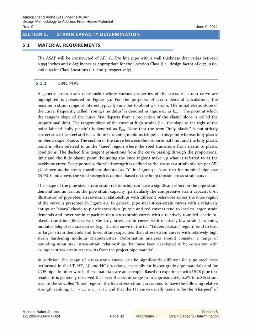
Alaska Stand Alone Gas Pipeline/ASAP Design Methodology to Address Frost Heave Potential Rev. 0 June 9, 2011
Michael Baker Jr., Inc. 121283-MBJ-RPT-024 Page 32
Section 5 Proprietary Strain Capacity Determination
SECTION 5. STRAIN CAPACITY DETERMINATION
5.1 MATERIAL REQUIREMENTS
The ASAP will be constructed of API 5L X70 line pipe with a wall thickness that varies between 0.595 inches and 0.857 inches as appropriate for the Location Class (i.e., design factor of 0.72, 0.60, and 0.50 for Class Locations 1, 2, and 3, respectively).
5.1.1 LINE PIPE
A generic stress-strain relationship where various properties of the stress vs. strain curve are highlighted is presented in Figure 5.1. For the purposes of strain demand calculations, the maximum strain range of interest typically runs out to about 2% strain. The initial elastic slope of the curve, frequently called “Young’s modulus” is denoted in Figure 5.1 as Estart. The point at which the tangent slope of the curve first departs from a projection of the elastic slope is called the proportional limit. The tangent slope of the curve at high strains (i.e., the slope to the right of the point labeled “fully plastic”) is denoted as Eend. Note that the term “fully plastic” is not strictly correct since the steel still has a finite hardening modulus (slope) at this point whereas fully plastic implies a slope of zero. The section of the curve between the proportional limit and the fully plastic point is often referred to as the “knee” region where the steel transitions from elastic to plastic conditions. The dashed line tangent projections from the curve passing through the proportional limit and the fully plastic point (bounding the knee region) make up what is referred to as the backbone curve. For pipe steels, the yield strength is defined as the stress at a strain of 0.5% per API 5L, shown as the stress coordinate denoted as “Y” in Figure 5.1. Note that for nominal pipe size (NPS) 8 and above, the yield strength is defined based on the hoop tension stress-strain curve.
The shape of the pipe steel stress-strain relationship can have a significant effect on the pipe strain demand and as well as the pipe strain capacity (particularly the compressive strain capacity). An illustration of pipe steel stress-strain relationships with different behaviors across the knee region of the curve is presented in Figure 5.2. In general, pipe steel stress-strain curves with a relatively abrupt or “sharp” elastic-to-plastic transition (purple and red curves) tend to lead to larger strain demands and lower strain capacities than stress-strain curves with a relatively rounded elastic-to-plastic transition (blue curve). Similarly, stress-strain curves with relatively low strain hardening modulus (slope) characteristics (e.g., the red curve in the flat “Lüders plateau” region) tend to lead to larger strain demands and lower strain capacities than stress-strain curves with relatively high strain hardening modulus characteristics. Deformation analyses should consider a range of bounding input steel stress-strain relationships that have been developed to be consistent with exemplar stress-strain test results from the project pipe material.
In addition, the shape of stress-strain curves can be significantly different for pipe steel tests performed in the LT, HT, LC and HC directions, especially for higher grade pipe materials and for UOE pipe. In other words, these materials are anisotropic. Based on experience with UOE pipe test results, it is generally observed that over the strain range from approximately 0.2% to 0.8% strain (i.e., in the so-called “knee” region), the four stress-strain curves tend to have the following relative strength ranking: HT > LC ≥ LT > HC and that the HT curve usually tends to be the “sharpest” of
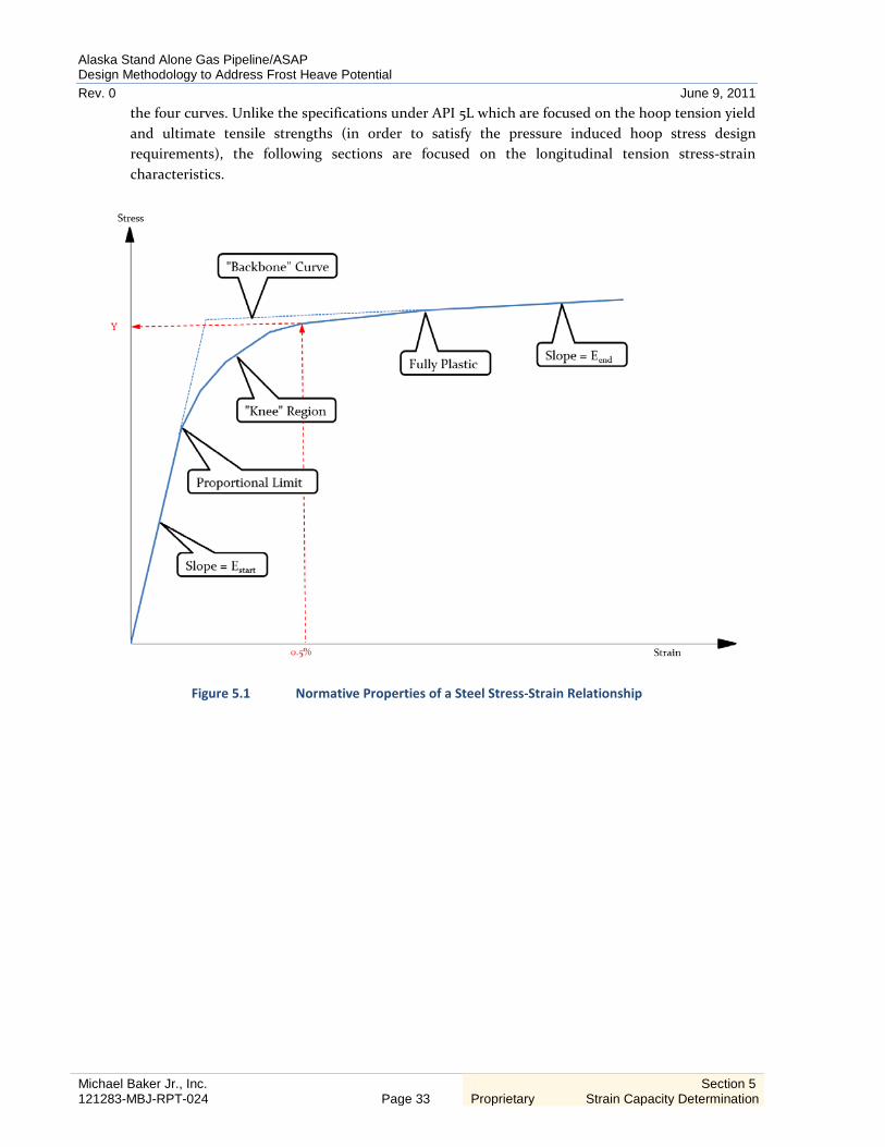
Alaska Stand Alone Gas Pipeline/ASAP Design Methodology to Address Frost Heave Potential Rev. 0 June 9, 2011
Michael Baker Jr., Inc. 121283-MBJ-RPT-024 Page 33
Section 5 Proprietary Strain Capacity Determination
the four curves. Unlike the specifications under API 5L which are focused on the hoop tension yield and ultimate tensile strengths (in order to satisfy the pressure induced hoop stress design requirements), the following sections are focused on the longitudinal tension stress-strain characteristics.
Figure 5.1 Normative Properties of a Steel Stress-Strain Relationship

Alaska Stand Alone Gas Pipeline/ASAP Design Methodology to Address Frost Heave Potential Rev. 0 June 9, 2011
Michael Baker Jr., Inc. 121283-MBJ-RPT-024 Page 34
Section 5 Proprietary Strain Capacity Determination
Figure 5.2 Illustration of Differing Stress-Strain Behavior in the Knee Region
(1) MINIMUM LONGITUDINAL YIELD STRENGTH
As noted above, the longitudinal tension (LT) stress-strain curves tend to be slightly weaker than the hoop tension (HT) stress strain curves in the knee region (e.g., in the region where yielding is defined). In many cases, the LT yield stress is actually below the specified minimum yield strength. This is not normally a cause for concern since as previously noted, the pipe SMYS is defined in the hoop tension direction.
(2) LONGITUDINAL TENSILE STRENGTH
Consideration will be given to specifying a minimum longitudinal tensile strength, as well as to specifying a relative low yield to tensile ratio to ensure a sufficient work hardening rate to avoid strain localization.
(3) MINIMUM UNIFORM LONGITUDINAL ELONGATION
Likewise, consideration will be given to specifying a minimum uniform longitudinal elongation to further avoid strain localization.

Alaska Stand Alone Gas Pipeline/ASAP Design Methodology to Address Frost Heave Potential Rev. 0 June 9, 2011
Michael Baker Jr., Inc. 121283-MBJ-RPT-024 Page 35
Section 5 Proprietary Strain Capacity Determination
(4) LONGITUDINAL STRESS-STRAIN CURVE
Basic pipe mill certificates will always provide a direct characterization of the yield and ultimate strengths in order to demonstrate that the material meets the specified minimum strength requirements. For ASAP strain-based design, it is anticipated that representative fully digital stress-strain curves will be obtained from both the LT and HT directions. It may also be desirable to obtain representative LC stress-strain curves.
Given the digital stress-strain data from representative pipe samples, it will be straight-forward to compute various measures of anisotropy such as the ratio of HT/LT yield and ultimate strengths or strengths at several selected strain levels of interest (e.g., at 1.5%, 2%, etc.). It will also be possible to compute various measures of curve shape or sharpness for the different curve directions such as the ratio of strengths at different levels of strain across the knee region and/or the plastic complementary energy at various levels of strain. These parameters can be used to characterize the variability of the project stress-strain relationships.
(5) LUDERS PLATEAU
Localized bands of plastic deformation may occur in certain materials before fracture. These bands are commonly referred to as Lüders bands as they were first reported by Guillaume Piobert and W. Lüders. These localization deformations result in a slight drop in strength below the initial yield strength, which is maintained for a moderate increase in imposed strain. The overall range of formation of the bands may form a flat yield, or Lüders, plateau.
Increasing imposed strain beyond the end of the plateau results in an increase in strength through strain-hardening. Strain-hardening continues to a peak that typically exceeds the yield strength by thirty to sixty percent.
For strain-based design applications, it is advisable to avoid excessive sharpness in the knee region of the stress-strain curves from any direction (e.g., LT or HT) and also to avoid a Lüder’s plateau. These characteristics can significantly increase the pipe strain demand (while at the same time decreasing the pipe strain capacity).
5.1.2 COATING EFFECT
Strain aging of pipe (e.g., due to heating during coating application) can tend to increase the sharpness of the knee region particularly for the HT curve with higher temperatures leading to higher levels of sharpness. Strain aging is also known to increase the pipe yield and ultimate strengths. Because strain aging tends to increase the yield strength more than it increases the ultimate tensile strength, it also tends to reduce the strain hardening modulus (i.e., as characterized by the Y/T ratio and/or the slope parameter Eend) in the region of interest for strain demand. For these reasons, it may be desirable to develop pipe specifications that include review of both as-received and aged stress-strain curves as well as to limit the heat to which the pipe is exposed during coating application if practicable.

Alaska Stand Alone Gas Pipeline/ASAP Design Methodology to Address Frost Heave Potential Rev. 0 June 9, 2011
Michael Baker Jr., Inc. 121283-MBJ-RPT-024 Page 36
Section 5 Proprietary Strain Capacity Determination
5.1.3 DIMENSIONAL CONTROL
Dimensional imperfections within a single length of line pipe can act as buckle initiation points and need to be minimized. However, the key concern for strain-based design is variation from pipe to pipe that acts as an imperfection and results in strain concentrations at girth welds. Any aspects of pipe geometry, such as ovality, variations in thickness, or tolerances in pipe diameter, that can result in misalignment across the weld can impact strain capacity. This is particularly true for thicker pipes, where internal or external alignment clamps may not be able to fully 'round out' pipe for welding.
5.1.4 GIRTH WELDS
Several welding techniques can be employed on girth welds joining lengths of pipe together. All have some impact on strain capacity. For example, GMAW with low CO2 content shielding gases produces the best combinations of strength and toughness but can be prone to generation of long defects if the welding procedure is not adequately optimized prior to field deployment. It is commonly used for mainline girth welding of long, large diameter pipelines. The various torch configurations such as single torch, dual torch, tandem wire, etc., also have implication on strain capacity. Single torch welding tends to give better results due to the lower heat input, but can affect construction efficiency and pipeline cost, especially in the arctic regions where the construction period is limited and logistics are challenging. Again, a well-balanced approach is needed to select the appropriate welding processes for the double jointing, mainline, tie-in, and infield repair procedures. The requirements of selecting welding procedures for these different types of welds to achieve both high strength and toughness may be challenging. The selected welding processes will need to be properly qualified and tested to confirm that the required strain capacity is met reliably.
5.1.5 WELD OVERMATCH
The key difference between welding for typical pipelines and those subject to high strain is the need for substantial and reliable strength overmatch of the weld metal relative to the base pipe. Reliable overmatch is critical for ensuring flaw tolerance adequate to allow for cost effective pipeline construction while ensuring safe design. This has been demonstrated in full-scale pressurized testing, where high weld overmatch was able to prevent failure at a large manufactured defect, resulting in fracture in the pipe body instead of the welds at high strain. The level of yield strength overmatch required to ensure a safe design depends on project-specific factors such as pipe grade, pipe geometry, flaw acceptance criteria, and the required strain capacity.
5.1.6 WELDMENT TOUGHNESS
Toughness of the weld metal and heat affected zone are critical to strain-based pipeline performance. Upper shelf behavior is required to resist fracture initiation by cleavage. It is also important to ensure adequate upper shelf toughness, which relates to ductile tearing resistance. The Charpy impact test is an excellent tool for assessing toughness and providing a quality check during weld procedure qualifications but is not sufficient for the detailed engineering of strain-

Alaska Stand Alone Gas Pipeline/ASAP Design Methodology to Address Frost Heave Potential Rev. 0 June 9, 2011
Michael Baker Jr., Inc. 121283-MBJ-RPT-024 Page 37
Section 5 Proprietary Strain Capacity Determination
based design pipelines. For these applications, fracture mechanics tests, such as the crack tip opening displacement (CTOD) test, should also be used to ensure adequate resistance to fracture with weld imperfections. Achieving high toughness in small scale testing is necessary but not sufficient to ensure a safe and cost effective strain-based design. The relationship between small scale toughness and full scale performance at high strain has not been adequately established by industry.
5.2 TESTING REQUIREMENTS
A number of small-scale and full-scale tests will be conducted to assist in determining the actual strain capacity of the line pipe to be used on the Project.
5.2.1 CURVED WIDE PLATE TESTING
Curved Wide Plate Testing (CWPT) has been used by industry as a proof test for qualifying strain-based design for many years. The test specimen consists of a large dog bone shape samples cut from a pipe containing the specific girth weld to be qualified. A flaw is saw-cut or electrical discharge machined (EDM) into the desired zone of the weld, and the specimen is pulled to failure in tension. Unfortunately, CWPT is not capable of quantifying the effect of biaxial loading due to internal pressure. It is also impractical to use CWPT to evaluate the effect of high-low misalignment on strain capacity. Recent full scale data have shown that these effects on strain capacity can be very significant. However, CWPT is still considered a cost effective and useful test for line pipe and weld procedure qualification and to establish initial estimates of the strain capacity.
5.2.2 FULL-SCALE TENSION TESTING
Although research is underway to develop suitable alternatives, pressurized full-scale tension testing remains the only fully validated method to confirm tensile strain capacity. If a limited number of tests are planned, an effective strategy is to use these tests to examine lower bound behavior. The goal is to confirm that the design meets the strain demand requirement when the key parameters are at the extremes of the acceptable construction envelope. Care should be taken to select test samples representative of the worst expected combination of the key fabrication parameters. On the other hand, selecting overly conservative parameters can result in an undesirable outcome. Another consideration is the availability of test frames to conduct these full scale tests. At this time, 30-inch pipe with a 0.630-inch wall thickness is near the limit of testing capability, which should be adequate for ASAP. Full-scale bend tests with internal pressure have been used, but are less efficient due to the limited weld length reaching the maximum strain. Additionally, modeling of the load/response behavior can be very challenging relative to a tension test.

Alaska Stand Alone Gas Pipeline/ASAP Design Methodology to Address Frost Heave Potential Rev. 0 June 9, 2011
Michael Baker Jr., Inc. 121283-MBJ-RPT-024 Page 38
Section 5 Proprietary Strain Capacity Determination
5.2.3 COMPRESSIVE STRAIN VALIDATION
Industry has developed and validated empirical equations and finite element modeling methods for estimating the compressive strain capacity of pipelines. The most widely used measure of pipe compressive strain capacity is that associated with the peak moment from an imposed curvature test on a full-scale pipe specimen or finite element analysis of a pipe stub section. Note that this strain limit is a serviceability limit state with a significant post-wrinkling reserve margin before the pipe pressure integrity is compromised (usually due to the development of high local strains within the wrinkle(s)). Empirical equations of this sort will be used to establish preliminary pipeline compressive strain capacity. Finite element analyses (FEA), and possibly pressurized full-scale bend tests, will be conducted to establish the compressive strain capacity. These studies will account for the effects of pipe anisotropy, material work hardening characteristics, girth weld misalignment or high-low, internal pressure fluctuations, axial loading, and thermal aging. The FEA method will be the primary tool to quantify the effect of variability in all major parameters; full-scale bend or buckling tests will only be used to validate the finite element models and provide useful experimental design data, if deemed necessary. A large number of finite element analyses may be required to cover a full range of parametric studies in support of a design reliability assessment. Because the compressive strain is defined over a certain gauge length (typically one to two pipe diameters), the selection of gauge length will accommodate geometric deformation effect and ensure the practical strain detectability by ILI tools. A common gauge length in finite element compressive strain capacity assessment, strain demand assessment, operation ILI monitoring, and any full-scale bend tests will be used.
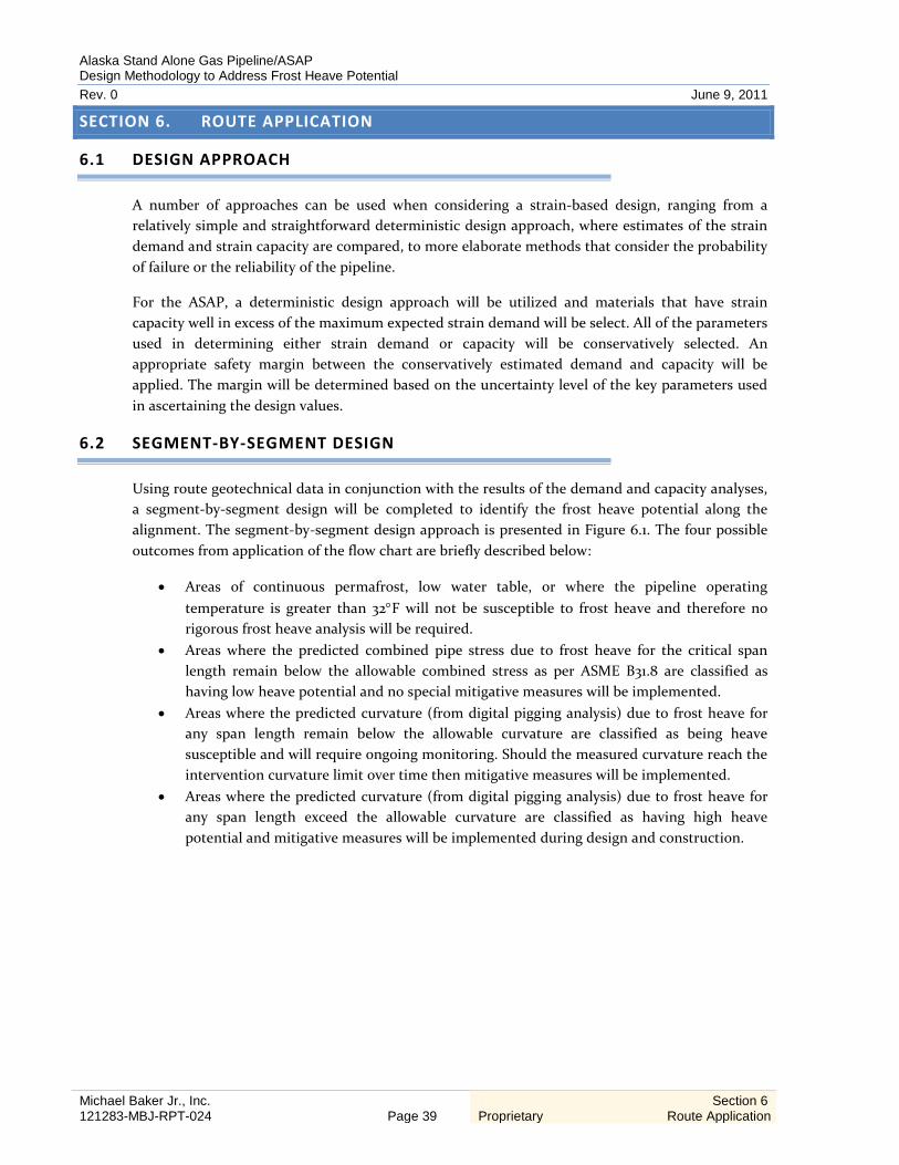
Alaska Stand Alone Gas Pipeline/ASAP Design Methodology to Address Frost Heave Potential Rev. 0 June 9, 2011
Michael Baker Jr., Inc. 121283-MBJ-RPT-024 Page 39
Section 6 Proprietary Route Application
SECTION 6. ROUTE APPLICATION
6.1 DESIGN APPROACH
A number of approaches can be used when considering a strain-based design, ranging from a relatively simple and straightforward deterministic design approach, where estimates of the strain demand and strain capacity are compared, to more elaborate methods that consider the probability of failure or the reliability of the pipeline.
For the ASAP, a deterministic design approach will be utilized and materials that have strain capacity well in excess of the maximum expected strain demand will be select. All of the parameters used in determining either strain demand or capacity will be conservatively selected. An appropriate safety margin between the conservatively estimated demand and capacity will be applied. The margin will be determined based on the uncertainty level of the key parameters used in ascertaining the design values.
6.2 SEGMENT-BY-SEGMENT DESIGN
Using route geotechnical data in conjunction with the results of the demand and capacity analyses, a segment-by-segment design will be completed to identify the frost heave potential along the alignment. The segment-by-segment design approach is presented in Figure 6.1. The four possible outcomes from application of the flow chart are briefly described below:
• Areas of continuous permafrost, low water table, or where the pipeline operating temperature is greater than 32°F will not be susceptible to frost heave and therefore no rigorous frost heave analysis will be required.
• Areas where the predicted combined pipe stress due to frost heave for the critical span length remain below the allowable combined stress as per ASME B31.8 are classified as having low heave potential and no special mitigative measures will be implemented.
• Areas where the predicted curvature (from digital pigging analysis) due to frost heave for any span length remain below the allowable curvature are classified as being heave susceptible and will require ongoing monitoring. Should the measured curvature reach the intervention curvature limit over time then mitigative measures will be implemented.
• Areas where the predicted curvature (from digital pigging analysis) due to frost heave for any span length exceed the allowable curvature are classified as having high heave potential and mitigative measures will be implemented during design and construction.

Alaska Stand Alone Gas Pipeline/ASAP Design Methodology to Address Frost Heave Potential Rev. 0 June 9, 2011
Michael Baker Jr., Inc. 121283-MBJ-RPT-024 Page 40
Section 6 Proprietary Route Application
Figure 6.1 Frost Heave Route Assessment Flow Chart
NO
YES Continuous Permafrost
?
No Heave
YES
YES
Operating Temp
>32°F?
Low Water Table?
YES
Low Heave
Frost Heave Critical Span
Stress < Allowable?
YES
Heave Susceptible
Frost Heave Any Span
Curvature > Allowable?
NO
High Heave
Start
NO
NO
NO

Alaska Stand Alone Gas Pipeline/ASAP Design Methodology to Address Frost Heave Potential Rev. 0 June 9, 2011
Michael Baker Jr., Inc. 121283-MBJ-RPT-024 Page 41
Section 6 Proprietary Route Application
6.3 POTENTIAL DESIGN MITIGATIVE MEASURES
For those pipeline route segments where the estimated heave potential may exceed the ability of the pipe to withstand the imposed displacement, a number of mitigative options, or combinations of options, could be employed to reduce the potential for deleterious movement including:
• Reroute within the alignment corridor to a non-frost-susceptible terrain unit, if available; • Investigate the subsurface of the suspect terrain segment more closely so as to reduce the
conservatism inherent in the station to station approach; • Change the operating temperature profile of the segment so as to reduce the freeze
potential, e.g., by adding heater stations, cycling the temperature, etc.; • Insulate the pipe ditch to reduce the heat flux through the frost-susceptible soil; • Increase the pipe wall thickness to increase the resistance of the pipe to ditch
displacements, as well as increasing the ability of the pipe to withstand higher displacements;
• Over-excavate the frost-susceptible soil beneath the buried pipeline and replace with non-frost-susceptible soils;
• Excavate soils with high uplift resistance above the pipe springline and replace with soils with low uplift resistance;
• Elevate the pipeline aboveground placing it in an embankment. Elevating the pipe would reduce or eliminate the heat extracted from the ground;
• Elevate the pipeline aboveground placing it on overhead supports. Elevating the pipe would eliminate the heat extracted from the ground and uncouple the pipe from the soil resistance;
• Heat trace the soil underneath the pipe to counteract frost penetration; • Emplace stand-alone heat pipes to freeze the soil quickly, reducing the ability of the frost-
susceptible soil to cause large soil volume changes; and • Combine compatible concepts presented above.

Alaska Stand Alone Gas Pipeline/ASAP Design Methodology to Address Frost Heave Potential Rev. 0 June 9, 2011
Michael Baker Jr., Inc. 121283-MBJ-RPT-024 Page 42
Section 7 Proprietary Construction Related Issues
SECTION 7. CONSTRUCTION RELATED ISSUES
7.1 WELDING PROCEDURES
To ensure high quality welds, a reasonable amount of flexibility is needed in welding parameters to allow welders the ability to manipulate the process and reduce the likelihood of producing unacceptable weld imperfections. The acceptable ranges of parameter variability that are intended to provide the performance that is similar to the completed qualification test welds will be established.
Weld qualification testing will bound the variability of critical parameters. In particular, heat input is critical because heat input modifies the metallurgical features of the HAZ and weld metal. Weld procedures will be qualified to a full suite of small scale tests and may also include large scale performance testing such as curved wide plates or full-scale tension tests with artificial defects. A test program that confirms the adequacy of the welds to provide resistance to fracture with a weld defect at the extreme of the welding process parameters acceptable during construction will be conducted.
7.2 AUTOMATED ULTRASONIC TESTING
Qualification of inspection equipment is critical to the successful implementation of a strain-based design for the pipeline. Materials qualification for strain-based design is intimately tied to the establishment of defect acceptance criteria with height and length restrictions. Radiographic testing does not give qualitative information about defect height and is therefore not suitable for a strain-based design. In order to determine both defect height and length with confidence, automated ultrasonic testing (AUT) will be required. A qualification program will be required to establish not only the detection capability, but also the sizing accuracy of the AUT system to be used during construction. The AUT system will be capable of detecting the critical defect height with high confidence. The sizing error of the system will be established for the range of defect dimensions at the acceptance limit. This error will be subtracted from the critical defect size to establish the acceptance criteria to be used during pipeline welding.

Alaska Stand Alone Gas Pipeline/ASAP Design Methodology to Address Frost Heave Potential Rev. 0 June 9, 2011
Michael Baker Jr., Inc. 121283-MBJ-RPT-024 Page 43
Section 8 Proprietary Operations and Maintenance
SECTION 8. OPERATIONS AND MAINTENANCE
8.1 MONITORING POTENTIAL FROST HEAVE
During design the frost heave potential along the alignment will be evaluated using the available route alignment data combined with the line pipe capacities and advanced engineering simulation methodology to explore the potential interaction between the soil subsurface and the pipe during its operational life. To address the differential values along the route, soil displacements and resistance values will be estimated using the landform characteristics along the route derived from the project geo-database. Scrutiny will continue throughout the operational life of the pipeline.
A key consideration in any strain-based pipeline design is the “monitor and maintain” component of the design philosophy. Periodic monitoring of the pipeline will identify locations that are of concern with respect to the pipe structural integrity. The monitoring interval is selected such that there will be enough time to plan and undertake intervention prior to the pipe experiencing a loss of structural integrity.
The best way to monitor curvature along ASAP is through periodic ILI surveys. An ILI geometry survey provides the most practicable and reliable way to accurately characterize the geometry of the entire length of the pipeline. Use of a high resolution inertial navigation system (INS) based geometry tool will result in the highest possible level of survey accuracy.
Several ILI vendors offer high resolution INS tools. The instrumentation on these tools includes a strap down, tri-axial fiber optic gyroscope based Inertial Measurement Unit (IMU), a tri-axial accelerometer, an odometer as well as a multi-arm mechanical caliper. The gyroscopes measure the change in orientation of the pig in terms of the pitch, azimuth, and roll angles; the odometer measures the along-the-pipe distance coordinate tie-points; and the calipers measure pipe ovality or dents and also locate the pipeline girth welds. The gyroscope and odometer data can be numerically differentiated to compute the pipeline curvature (which is proportional to the bending strain) or numerically integrated to estimate the pipe position between coordinate tie-points. Typical accuracies of inertial survey tools are as follows:
• Curvature Detection: ±0.02% Strain • Bend Angle Detection: ±0.1o • Dent/Ovality: ±2.5 mm • Weld-to-Weld Distance: ±12.5 mm • Mapping Accuracy 1:2000 (depends on distance between coordinate tie-points)
Since the early 1990’s, the pipeline industry has gained experience with these tools and they have become a key component of pipeline systems which incorporate the “monitor and maintain” component of the strain-based design philosophy. While the pipeline (X-Y-Z) position mapping is useful for GIS applications and pipeline location, the most important result from an inertial survey of a pipeline for structural integrity assessments is the curvature/bending strain not associated with intentional bends. The caliper data can also be extremely useful for establishing out-of-roundness and incipient wrinkling deformations of the pipe wall at high curvature/bending strain locations.
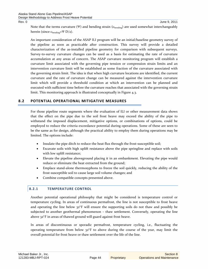
Alaska Stand Alone Gas Pipeline/ASAP Design Methodology to Address Frost Heave Potential Rev. 0 June 9, 2011
Michael Baker Jr., Inc. 121283-MBJ-RPT-024 Page 44
Section 8 Proprietary Operations and Maintenance
Note that the terms curvature (Ψ) and bending strain (εbending) are used somewhat interchangeably herein (since εbending=Ψ D/2).
An important consideration of the ASAP ILI program will be an initial/baseline geometry survey of the pipeline as soon as practicable after construction. This survey will provide a detailed characterization of the as-installed pipeline geometry for comparison with subsequent surveys. Survey-to-survey curvature changes can be used as a basis for estimating the rate of curvature accumulation at any areas of concern. The ASAP curvature monitoring program will establish a curvature limit associated with the governing pipe tension or compression strain limits and an intervention curvature limit will be established as some fraction of the curvature associated with the governing strain limit. The idea is that when high curvature locations are identified, the current curvature and the rate of curvature change can be measured against the intervention curvature limit which will provide a threshold condition at which an intervention can be planned and executed with sufficient time before the curvature reaches that associated with the governing strain limit. This monitoring approach is illustrated conceptually in Figure 4.3.
8.2 POTENTIAL OPERATIONAL MITIGATIVE MEASURES
For those pipeline route segments where the evaluation of ILI or other measurement data shows that the effect on the pipe due to the soil frost heave may exceed the ability of the pipe to withstand the imposed displacement, mitigative options, or combinations of options, could be employed to reduce the criteria exceedance potential during operations. Some of these are seen to be the same as for design, although the practical ability to employ them during operations may be limited. The options include:
• Insulate the pipe ditch to reduce the heat flux through the frost-susceptible soil; • Excavate soils with high uplift resistance above the pipe springline and replace with soils
with low uplift resistance; • Elevate the pipeline aboveground placing it in an embankment. Elevating the pipe would
reduce or eliminate the heat extracted from the ground; • Emplace stand-alone thermosyphons to freeze the soil quickly, reducing the ability of the
frost-susceptible soil to cause large soil volume changes; and • Combine compatible concepts presented above.
8.2.1 TEMPERATURE CONTROL
Another potential operational philosophy that might be considered is temperature control or temperature cycling. In areas of continuous permafrost, the line is not susceptible to frost heave and operating the line below 32°F will ensure the supporting soils do not thaw and possibly be subjected to another geothermal phenomenon – thaw settlement. Conversely, operating the line above 32°F in areas of thawed ground will guard against frost heave.
In areas of discontinuous or sporadic permafrost, temperature cycling, i.e., fluctuating the operating temperature from below 32°F to above during the course of the year, may limit the overall potential for frost heave or thaw settlement over the life of the line.

Alaska Stand Alone Gas Pipeline/ASAP Design Methodology to Address Frost Heave Potential Rev. 0 June 9, 2011
Michael Baker Jr., Inc. 121283-MBJ-RPT-024 Page 45
Section 8 Proprietary Operations and Maintenance
8.2.2 LINE LEVELING
Line-leveling is one possible form of intervention/mitigation that can be employed should the measured curvature approach or exceed the curvature limits established for the project. This would entail excavating the line in areas experiencing frost heave and re-leveling the line to reduce the curvature.

Alaska Stand Alone Gas Pipeline/ASAP Design Methodology to Address Frost Heave Potential Rev. 0 June 9, 2011
Michael Baker Jr., Inc. 121283-MBJ-RPT-024 Page 46
Section 9 Proprietary Conclusion
SECTION 9. CONCLUSION
The design approach to frost heave explained in this report is summarized in Figure 1.3 which shows the flow of the various steps needed to define and begin the assembly of the components of the project approach in preliminary design; finalize the assembly and verification and apply the approach to the alignment in final design; and continue route monitoring and potential mitigation throughout operations. In the current front end loading phase of the project, the design approach is being developed and scoped of initiation during the next phase - preliminary design.
Although only the approach to frost heave is developed in this report, the approach is illustrative of the design approach to other displacement loadings that may cause longitudinal stress in the pipe such as thaw settlement.
AGDC is committed to the complete development and verification of the design approach for application throughout the design life. As the development progresses, AGDC will share the ongoing verification and application studies with PHMSA throughout this process to ensure concurrence and heighten confidence in the safety and integrity of the pipeline.
Alaska Stand Alone Gas Pipeline/ASAP Design Methodology to Address Frost Heave Potential Rev. 0 June 9, 2011
Michael Baker Jr., Inc. 121283-MBJ-RPT-024 Page 47
Section 10 Proprietary References
SECTION 10. REFERENCES
Andersland, Orland B. and Branko Ladanyi. 2004. Frozen Ground. 2nd Edition. Published in cooperation with ASCE Press. John Wiley & Sons, Inc. Table 2-7.
ASCE. 1984. “Guidelines for the Seismic Design of Oil and Gas Pipeline Systems.” Committee on Gas and Liquid Fuel Lifelines.
Bureau of Land Management (BLM). 2002. Final Environmental Impact Statement Renewal of the Grant for the Trans-Alaska Pipeline System Right-of-Way. Environmental Impact Statement, Department of the Interior, Bureau of Land Management.
COLTKBR. 2003. “Conceptual Geotechnical/Geothermal Design Basis.” Rev. B. http://www.ngps.nt.ca/Upload/Proponent/Imperial%20Oil%20Resources%20Ventures%20Limited/050922_IORVL_to_JRP_R2_Q39-45-geo.pdf
COLTKBR. 2007. “Frost Heave Structural Analysis of the Ochre River HDD Crossing.” Rev. 1. https://www.neb-one.gc.ca/ll-eng/livelink.exe?func=ll&objId=477649&objAction=browse
Hart, J.D., G. Antaki, et.al. 2001. “Guidelines for the Design of Buried Steel Pipe.” Published by the ASCE American Lifelines Alliance. www.americanlifelinesalliance.org.
Hart, J.D., G.H. Powell, and N. Zulfiqar. 1996. "A Material Model for Pipeline Steels.” ASME Offshore Mechanics and Offshore Engineering International Pipeline Conference. Calgary, Alberta, Canada.
Honegger, D.G., and D. J. Nyman. 2004. “Guidelines for the Seismic Design and Assessment of Natural Gas and Liquid Hydrocarbon Pipelines.” Pipeline Research Council International, Inc. Catalog No. L51927.
Konrad, J.M. and N.R. Morgenstern. 1981. “The Segregation Potential of a Freezing Soil”, Canadian Geotechnical Journal, 18: 482-491.
Mroz, Z. 1967. “On the Description of Anisotropic Work Hardening.” Journal of Mechanics, Physics and Solids, 15, 163-175.
Popov, E.P. 1976. “Mechanics of Materials.” 2nd Edition. Prentice Hall.
SSD, Inc. 2011. "PIPLIN-PC: Stress and Deformation Analysis of Pipelines." Version 4.58 Arctic, User Reference and Theoretical Manual, Reno, Nevada, February 2011 (Proprietary).

Alaska Stand Alone Gas Pipeline/ASAP Design Methodology to Address Frost Heave Potential Rev. 0 June 9, 2011
Michael Baker Jr., Inc. 121283-MBJ-RPT-024 Page A.1 Proprietary
Appendix A PHMSA Correspondence
APPENDIX A PHMSA CORRESPONDENCE
1. U.S. Department of Transportation, Pipeline and Hazardous Materials Safety Administration Letter to Mr. Bob Swenson, Alaska Stand Alone Pipeline, dated March 3, 2010
2. State of Alaska, Office of the Governor letter to Mr. Jeffrey Weise, Associate Administrator for Pipeline Safety, US Department of Transportation, dated April 12, 2010
3. U.S. Department of Transportation, Pipeline and Hazardous Materials Safety Administration Letter to Mr. Daniel Fauske, President Alaska Gasline Development Corporation, received May 4, 2010

Michael Baker Jr., Inc. 121283-MBJ-RPT-024 Page A.2 Appendix A PHMSA Correspondence
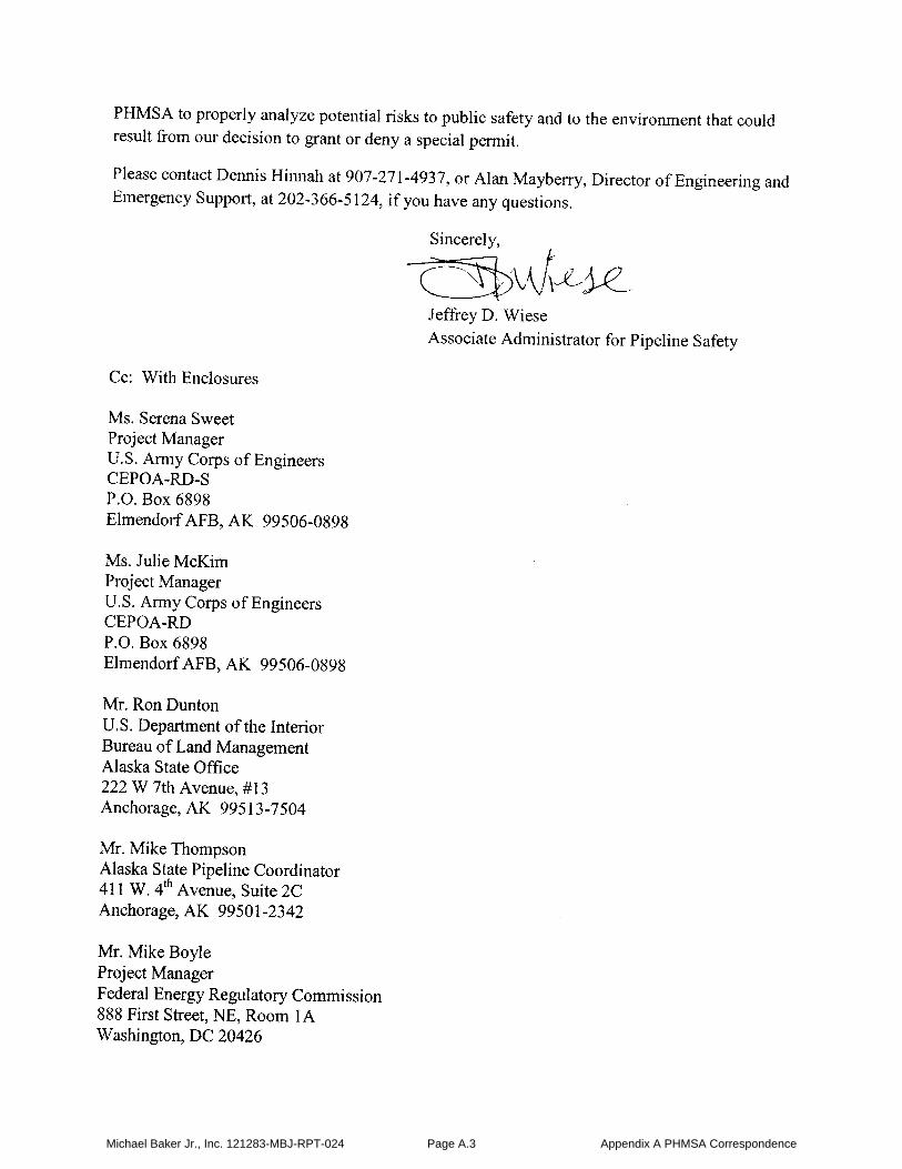
Michael Baker Jr., Inc. 121283-MBJ-RPT-024 Page A.3 Appendix A PHMSA Correspondence

Michael Baker Jr., Inc. 121283-MBJ-RPT-024 Page A.4 Appendix A PHMSA Correspondence

Michael Baker Jr., Inc. 121283-MBJ-RPT-024 Page A.5 Appendix A PHMSA Correspondence

Michael Baker Jr., Inc. 121283-MBJ-RPT-024 Page A.6 Appendix A PHMSA Correspondence
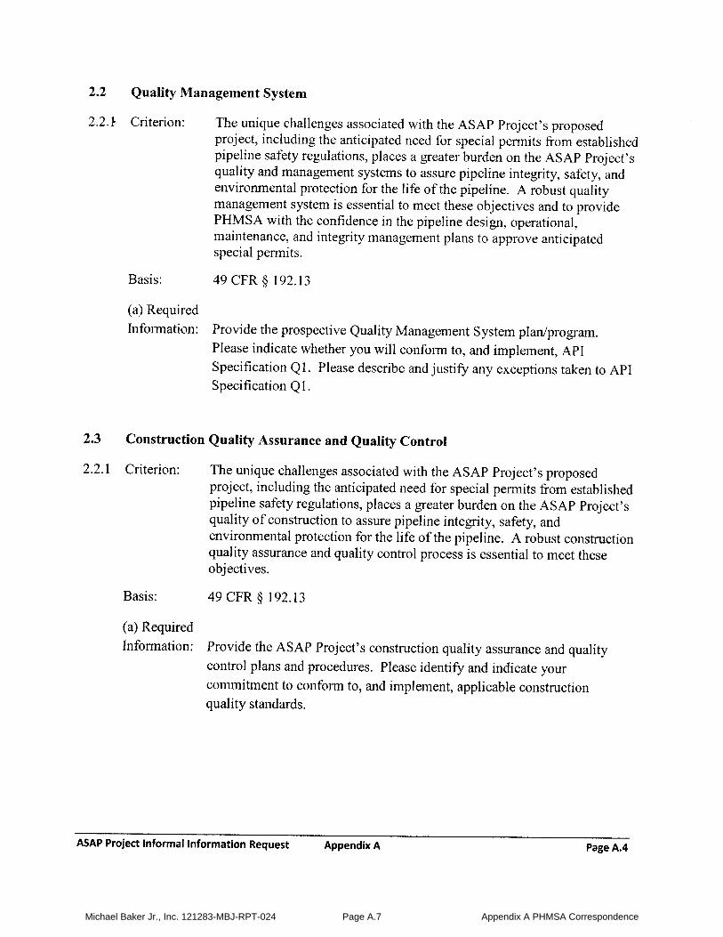
Michael Baker Jr., Inc. 121283-MBJ-RPT-024 Page A.7 Appendix A PHMSA Correspondence

Michael Baker Jr., Inc. 121283-MBJ-RPT-024 Page A.8 Appendix A PHMSA Correspondence

Michael Baker Jr., Inc. 121283-MBJ-RPT-024 Page A.9 Appendix A PHMSA Correspondence

Michael Baker Jr., Inc. 121283-MBJ-RPT-024 Page A.10 Appendix A PHMSA Correspondence

Michael Baker Jr., Inc. 121283-MBJ-RPT-024 Page A.11 Appendix A PHMSA Correspondence

Michael Baker Jr., Inc. 121283-MBJ-RPT-024 Page A.12 Appendix A PHMSA Correspondence

Michael Baker Jr., Inc. 121283-MBJ-RPT-024 Page A.13 Appendix A PHMSA Correspondence

Michael Baker Jr., Inc. 121283-MBJ-RPT-024 Page A.14 Appendix A PHMSA Correspondence

Michael Baker Jr., Inc. 121283-MBJ-RPT-024 Page A.15 Appendix A PHMSA Correspondence

Michael Baker Jr., Inc. 121283-MBJ-RPT-024 Page A.16 Appendix A PHMSA Correspondence
Michael Baker Jr., Inc. 121283-MBJ-RPT-024 Page A.17 Appendix A PHMSA Correspondence

Michael Baker Jr., Inc. 121283-MBJ-RPT-024 Page A.18 Appendix A PHMSA Correspondence

Michael Baker Jr., Inc. 121283-MBJ-RPT-024 Page A.19 Appendix A PHMSA Correspondence

Michael Baker Jr., Inc. 121283-MBJ-RPT-024 Page A.20 Appendix A PHMSA Correspondence
Michael Baker Jr., Inc. 121283-MBJ-RPT-024 Page A.21 Appendix A PHMSA Correspondence

Michael Baker Jr., Inc. 121283-MBJ-RPT-024 Page A.22 Appendix A PHMSA Correspondence
Michael Baker Jr., Inc. 121283-MBJ-RPT-024 Page A.23 Appendix A PHMSA Correspondence

Michael Baker Jr., Inc. 121283-MBJ-RPT-024 Page A.24 Appendix A PHMSA Correspondence

Michael Baker Jr., Inc. 121283-MBJ-RPT-024 Page A.25 Appendix A PHMSA Correspondence

Michael Baker Jr., Inc. 121283-MBJ-RPT-024 Page A.26 Appendix A PHMSA Correspondence

Michael Baker Jr., Inc. 121283-MBJ-RPT-024 Page A.27 Appendix A PHMSA Correspondence

Michael Baker Jr., Inc. 121283-MBJ-RPT-024 Page A.28 Appendix A PHMSA Correspondence

SEAN PARNELL P.O. Box 110001Governor Juneau, Alaska 99811-0001
(907) 465-3500Fax (907) 465-3532
STATE OF ALASKAOFFICE OF THE GOVERNOR
April 12,2010
Mr. Jeffrey D. WieseAssociate Administrator for Pipeline SafetyU.S Department of Transportation1200 New Jersey Avenue, SEWashington, DC 20590
Dear Mr. Wiese,
The Office of the Governor is in receipt of March 3, 2010 requesting information about the natureof the proposed Alaska In-State Gas Pipeline Project and plans for the project to submit waivers forcompliance with Federal Pipeline Safety Regulations under the federal standards you identified.
Our Office has reviewed Enclosure A included in your letter that requests information concerningspecial permits. I am enclosing a table with this letter which responds to each criterion youidentified. Please note a number of concerns raised in Enclosure A are related to procedures thathave been identified, or are under consideration by other proposed arctic natural gas pipelineproponents. The Alaska In-State Gas Pipeline Project (identified in your letter as the Alaska StandAlone Pipeline) is attempting to maintain a tight timeline in order to provide for the near termenergy needs of residents and commercial interests within the state of Alaska. Our team has madespecific efforts throughout our planning and initial engineering design to highlight issues that mightcause delay, and has worked hard to avoid the need for any request for submission of special permitapplications for the project pursuant to 49 C.F.R. Section 190.341. We believe there are no specialpermit applications required at this time, but will remain diligent in our review of such need.
For example, we are not requesting waivers for the Alaska In-State Gas Pipeline Project (identifiedin Enclosure A of your March 3, 2010 letter) for the following key permits:
• application of reliability based design and assessment;• deviation from depth of cover and valve spacing requirements;
• relief from post-construction hydrotest requirements;• alternative MAOP requirements; or• deviation from class location requirements.
Enclosure B to your letter contains “Guidance for Special Permit Applicants on ProvidingEnvironmental Information.” An Environmental Impact Statement (ElS) in accordance with theNational Environmental Policy Act (NEPA) is currently underway with the U.S. Army Corps ofEngineers USACE) as the lead federal agency with several other federal agencies acting ascooperating agencies. The ElS will assess potential risks to the public and the environment thatcould result from approval of the Alaska In-State Gas Pipeline Project. In the event that the AlaskaIn-State Gas Pipeline Project needs to deviate from one or more regulations, a special permit waiver
Michael Baker Jr., Inc. 121283-MBJ-RPT-024 Page A.29 Appendix A PHMSA Correspondence
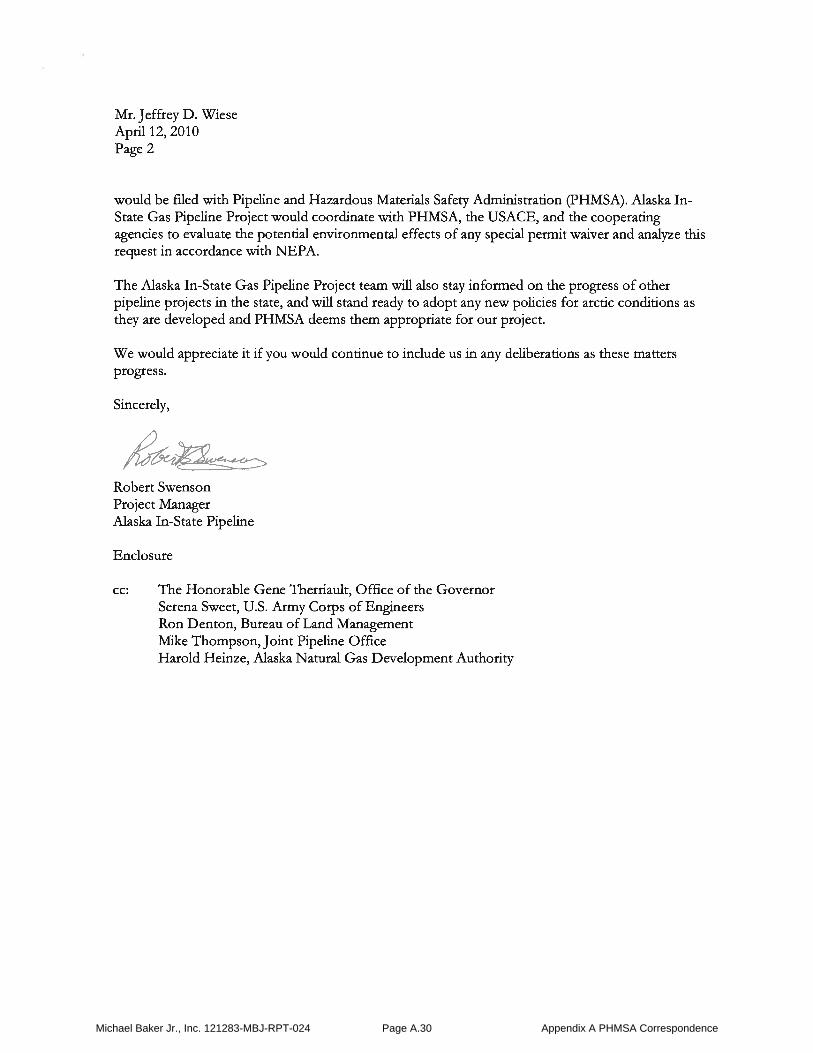
Mr. Jeffrey D. WieseApril 12, 2010Page 2
would be filed with Pipeline and Hazardous Materials Safety Administration (PHMSA). Alaska InState Gas Pipeline Project would coordinate with PHMSA, the USACE, and the cooperatingagencies to evaluate the potential environmental effects of any special permit waiver and analyze thisrequest in accordance with NEPA.
The Alaska In-State Gas Pipeline Project team will also stay informed on the progress of otherpipeline projects in the state, and will stand ready to adopt any new policies for arctic conditions asthey are developed and PHMSA deems them appropriate for our project.
We would appreciate it if you would continue to include us in any deliberations as these mattersprogress.
Sincerely,
Robert SwensonProject ManagerAlaska In-State Pipeline
Enclosure
cc: The Honorable Gene Therriault, Office of the GovernorSerena Sweet, U.S. Army Corps of EngineersRon Denton, Bureau of Land ManagementMike Thompson, Joint Pipeline OfficeHarold Heinze, Alaska Natural Gas Development Authority
Michael Baker Jr., Inc. 121283-MBJ-RPT-024 Page A.30 Appendix A PHMSA Correspondence
In-S
tate
Gas
Pipeline
Pro
ject
[A
lask
aS
tan
dA
lo
ne
Pip
elin
e(A
SA
P)]
PH
MS
AM
arch
3,
2010
Inform
ation
Request
-R
esp
on
se
Ou
tlin
e
Issu
eC
riterion
Su
mm
ary
Response
2.1.
1P
rovi
deP
HM
SA
wit
hsu
ffic
ient
info
rmat
ion
earl
yin
The
deta
iled
desi
gnph
ase
of
the
Ala
ska
Sta
ndA
lone
Pipe
line
(ASA
P)de
sign
proc
ess
proj
ect
issc
hedu
led
tost
art
in20
11.
2.2.
1Q
ualit
yM
anag
emen
tSy
stem
AQ
ualit
yM
anag
emen
tSy
stem
for
the
ASA
Ppr
ojec
tw
ould
beim
plem
ente
ddu
ring
deta
iled
desi
gn.
2.3.
1C
onst
ruct
ion
Qua
lity
Ass
uran
ceA
cons
truc
tion
QA
/QC
plan
wou
ldbe
deve
lope
dfo
rco
nstr
ucti
on,i
nco
njun
ctio
nw
ith
the
sele
cted
cons
truc
tion
cont
ract
ors.
3.1.
1R
elia
bilit
yB
ased
Des
ign
and
Ass
essm
ent
AR
elia
bilit
yB
ased
Des
ign
and
Ass
essm
ent
(RB
DA
)ap
proa
chis
not
prop
osed
for
use
byth
epr
ojec
t.3.
2.1
Stra
inB
ased
Des
ign
Stra
inba
sed
desi
gnfo
rin
tegr
ityas
sura
nce
for
arct
icge
ohaz
ard
pote
ntia
llo
adin
gsw
ould
bede
velo
ped,
asre
quir
ed,
inac
cord
wit
hA
mer
ican
Soci
ety
ofM
echa
nica
lE
ngin
eers
(ASM
E)
B31
.8,
Para
833.
5:“D
esig
nfo
rSt
ress
esG
reat
erth
anY
ield
”.3.
3.1
Add
itio
nalD
esig
nR
equi
rem
ents
for
Alt
erna
tive
No
spec
ial
perm
itfo
rth
efo
llow
ing
are
bein
gso
ught
:M
axim
umA
llow
able
Ope
rati
ngP
ress
ure
(MA
OP)
•cl
ass
loca
tion
requ
irem
ents
,or
•al
tern
ativ
eM
AO
P3.
4.1
Dep
tho
fC
over
No
spec
ial
perm
its
are
bein
gso
ught
for
devi
atio
nsfr
omde
pth
of
cove
r.3.
5.1
Val
veSp
acin
gN
osp
ecia
lpe
rmit
sar
ebe
ing
soug
htfo
rde
viat
ions
from
min
imum
bloc
kva
lve
spac
ing.
3.6.
1Pi
pelin
eC
ompo
nent
sN
osp
ecia
lpe
rmit
sar
ebe
ing
soug
htfo
rpi
pelin
eco
mpo
nent
s.4.
1.1
Stee
lP
ipe
Man
ufac
turi
ngS
peci
fica
tion
and
Qua
lity
The
spec
ific
atio
nsfo
rth
epr
opos
edX
70li
ne-p
ipe
will
been
sure
dto
mee
tal
lre
gula
tory
requ
irem
ents
and
PH
MS
Agu
idel
ines
.H
owev
er,
deta
iled
pipe
spec
ific
atio
nsan
dve
ndor
qual
ific
atio
nspi
pear
eno
tex
pect
edto
bead
dres
sed
until
the
deta
iled
desi
gnph
ase.
5.1.
1Q
uali
fica
tion
ofW
eldi
ngP
roce
dure
sW
eldi
ngre
quir
emen
tsw
ould
bede
velo
ped
duri
ngde
taile
dde
sign
.5.
2.1
Qua
lifi
cati
onof
Wel
ders
Wel
der
qual
ific
atio
nre
quir
emen
tsw
ould
besp
ecif
ied
inth
eco
nstr
ucti
onbi
d.5.
3.1
Wel
dA
ccep
tanc
eT
esti
ngan
dA
ccep
tanc
eC
rite
ria
No
spec
ial p
erm
its
are
bein
gso
ught
for
devi
atio
nsfr
ompost
cons
truc
tion
pres
sure
test
ing.
Page
1of
2
Michael Baker Jr., Inc. 121283-MBJ-RPT-024 Page A.31 Appendix A PHMSA Correspondence

Issu
eC
rite
rion
Sum
mar
yR
esponse
5.4.
1G
ener
alC
onst
ruct
ion
inA
rcti
cC
ondi
tion
sN
osp
ecia
lpe
rmit
sar
ebe
ing
soug
htfo
rde
viat
ions
from
post
-co
nstr
ucti
onpr
essu
rete
stin
g.Sp
ecia
lco
nstr
ucti
onpr
actic
esre
quir
edfo
rar
ctic
cond
itio
nsw
ould
bead
dres
sed
inth
eC
onst
ruct
ion
plan
and
Qua
lity
Ass
uran
ce&
Qua
lity
Con
trol
(QA
/QC
)m
anua
l.5.
5.1
Rec
ent
Con
stru
ctio
nIs
sues
Con
stru
ctio
npr
actic
esre
quir
edto
avoi
dpi
pequ
ality
issu
es,
and
tore
mec
liate
alli
dent
ifie
dde
fect
sw
ould
bead
dres
sed
inth
eC
onst
ruct
ion
plan
and
QA
/QC
man
ual.
5.6.
1A
ddit
iona
lC
onst
ruct
ion
Req
uire
men
tsN
osp
ecia
lpe
rmit
sfo
rth
efo
llow
ing
are
bein
gso
ught
:•
clas
slo
cati
onre
quir
emen
ts,
or•
alte
rnat
ive
MA
OP
6.1.
1E
xter
nal
Cor
rosi
onC
ontr
olE
xter
nal
corr
osio
nco
ntro
lw
ould
bead
dres
sed
duri
ngde
taile
dde
sign
6.2.
1In
tern
alC
orro
sion
Con
trol
Inte
rnal
corr
osio
nco
ntro
lw
ould
bead
dres
sed
duri
ngde
taile
dde
sign
7.1
Pos
tC
onst
ruct
ion
Pre
ssur
eT
est
No
spec
ial
perm
its
are
bein
gso
ught
for
devi
atio
nsfr
omhy
drot
est
requ
irem
ents
.
8.1.
1M
AO
PN
osp
ecia
lpe
rmit
sfo
rth
efo
llow
ing
are
bein
gso
ught
:•
clas
slo
cati
onre
quir
emen
ts,
or•
alte
rnat
ive
MA
OP
8.2.
1St
rain
mon
itor
ing
Ope
rati
onal
mon
itor
ing
tech
niqu
esw
ould
bede
velo
ped
inac
cord
wit
han
yst
rain
base
dde
sign
mea
sure
s8.
3.1
Rel
iabi
lity
Bas
edA
sses
smen
tA
Rel
iabi
lity
Bas
edD
esig
nan
dA
sses
smen
t(R
BD
A)
appr
oach
isno
tpr
opos
edfo
rus
eby
the
proj
ect.
9.1.
1Fa
ilure
Impa
ctZ
one
No
spec
ial
perm
its
are
bein
gso
ught
for
devi
atio
nsfr
omhy
drot
est
requ
irem
ents
.9.
2.1
Per
iodi
cIn
tegr
ity
Ass
essm
ents
No
spec
ial
perm
its
are
bein
gso
ught
for
devi
atio
nsfr
omhy
drot
est
requ
irem
ents
.9.
3.1
Pre
vent
ive
and
Miti
gativ
eM
easu
res
No
spec
ial
perm
its
are
bein
gso
ught
for
devi
atio
nsfr
omhy
drot
est
requ
irem
ents
.9.
4.1
Ris
kA
naly
sis
No
spec
ial
perm
its
are
bein
gso
ught
for
devi
atio
nsfr
omhy
drot
est
requ
irem
ents
.
Page
2of
2
Michael Baker Jr., Inc. 121283-MBJ-RPT-024 Page A.32 Appendix A PHMSA Correspondence

Michael Baker Jr., Inc. 121283-MBJ-RPT-024 Page A.33 Appendix A PHMSA Correspondence

Michael Baker Jr., Inc. 121283-MBJ-RPT-024 Page A.34 Appendix A PHMSA Correspondence
Michael Baker Jr., Inc. 121283-MBJ-RPT-024 Page A.35 Appendix A PHMSA Correspondence
Michael Baker Jr., Inc. 121283-MBJ-RPT-024 Page A.36 Appendix A PHMSA Correspondence

Michael Baker Jr., Inc. 121283-MBJ-RPT-024 Page A.37 Appendix A PHMSA Correspondence

Michael Baker Jr., Inc. 121283-MBJ-RPT-024 Page A.38 Appendix A PHMSA Correspondence

Michael Baker Jr., Inc. 121283-MBJ-RPT-024 Page A.39 Appendix A PHMSA Correspondence

Michael Baker Jr., Inc. 121283-MBJ-RPT-024 Page A.40 Appendix A PHMSA Correspondence
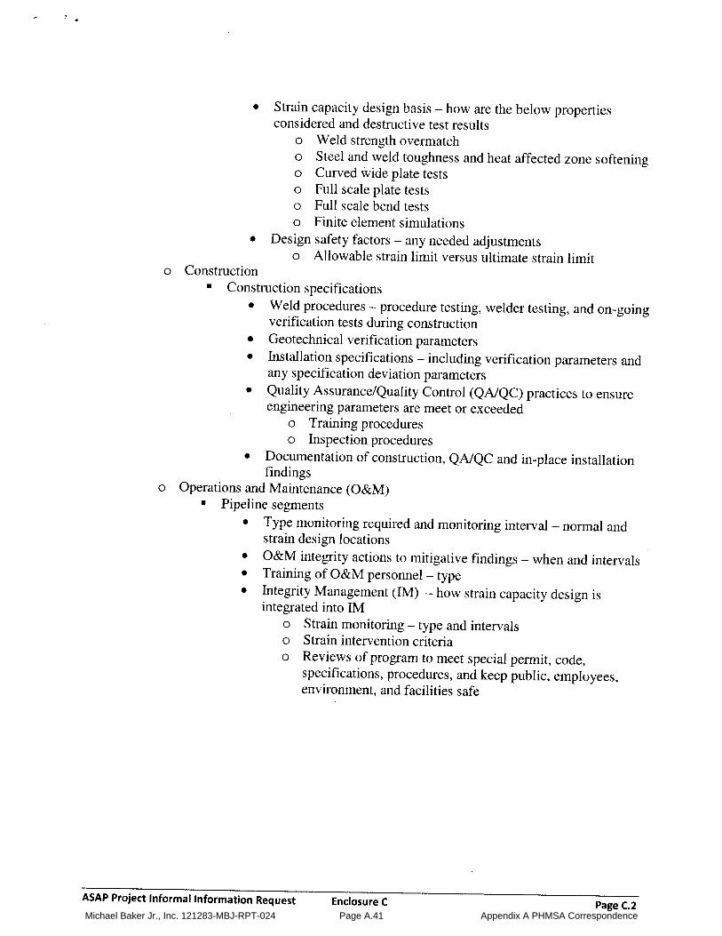
Michael Baker Jr., Inc. 121283-MBJ-RPT-024 Page A.41 Appendix A PHMSA Correspondence

Alaska Stand Alone Gas Pipeline/ASAP Design Methodology to Address Frost Heave Potential Rev. 0 June 9, 2011
Michael Baker Jr., Inc. 121283-MBJ-RPT-024 Page B.1 Proprietary
Appendix B Structural Mechanics of Buried Pipelines
APPENDIX B STRUCTURAL MECHANICS OF BURIED PIPELINES
Although some sections of the ASAP are aboveground, notably at waterway crossings and at the beginning of pipeline route on the North Slope, ASAP is primarily a buried pipeline. Buried pipelines are essentially “restrained,” that is, displacement of the pipe is restricted by the soil around it.
Engineering calculations typically address the pipe in a bi-axial stress state called plane stress. The active stresses considered in pipe engineering calculations are shown in Figure B. 1 – a hoop stress and strain which act around the circumference of the pipe, and a longitudinal stress and strain which are directed along the long axis of the pipe. In general, there is a third stress, a shear stress, which could be acting on the edges of the above unit section, but this is not normally significant and usually neglected in engineering calculations of transmission pipelines. Pipelines with diameter to wall thickness ratios (D/t) greater than 20, typical of transmission pipelines, are considered “thin-walled” as the distribution of normal stress perpendicular to the surface is essentially uniform throughout the wall thickness.
Figure B. 1 Pipe Stresses and Strains
The relation between stress (σ) and strain (ε) for pipeline steel when loaded in one direction (i.e., a unixial stress-strain curve) can be generally represented as shown in Figure B.2. Below the proportional limit, the stress is linearly related to the strain, a relation called Hooke’s law, given by:
εσ E= Equation B.1
with the constant “E” known as the Young’s modulus. The yield point for pipeline engineering is defined by testing requirements to be the point at which the specified minimum yield strength (SMYS) of the pipe is recorded – 0.5% strain. Note that this definition of the “yield” does not concisely fit classical “textbook” definitions of yield, which is often defined as the point at which non-recoverable, i.e. “plastic” deformations, initiate. For example, if the pipe material was considered to be governed by Hooke’s law to SMYS of 70 ksi, the associated strain would be only:
%237.0/00237.0//500,29/70 === ininininksiksiε
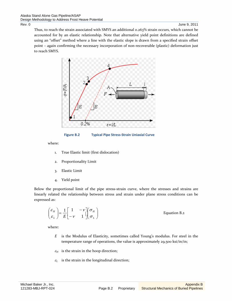
Alaska Stand Alone Gas Pipeline/ASAP Design Methodology to Address Frost Heave Potential Rev. 0 June 9, 2011
Michael Baker Jr., Inc. 121283-MBJ-RPT-024 Page B.2 Proprietary
Appendix B Structural Mechanics of Buried Pipelines
Thus, to reach the strain associated with SMYS an additional 0.263% strain occurs, which cannot be accounted for by an elastic relationship. Note that alternative yield point definitions are defined using an “offset” method where a line with the elastic slope is drawn from a specified strain offset point – again confirming the necessary incorporation of non-recoverable (plastic) deformation just to reach SMYS.
Figure B.2 Typical Pipe Stress-Strain Uniaxial Curve
where:
1. True Elastic limit (first dislocation)
2. Proportionality Limit
3. Elastic Limit
4. Yield point
Below the proportional limit of the pipe stress-strain curve, where the stresses and strains are linearly related the relationship between stress and strain under plane stress conditions can be expressed as:
−
−=
L
H
L
H
E σσ
νν
εε
111
Equation B.2
where:
E is the Modulus of Elasticity, sometimes called Young’s modulus. For steel in the temperature range of operations, the value is approximately 29,500 ksi/in/in;
εH is the strain in the hoop direction;
εL is the strain in the longitudinal direction;

Alaska Stand Alone Gas Pipeline/ASAP Design Methodology to Address Frost Heave Potential Rev. 0 June 9, 2011
Michael Baker Jr., Inc. 121283-MBJ-RPT-024 Page B.3 Proprietary
Appendix B Structural Mechanics of Buried Pipelines
σH is the stress in the hoop direction;
σL is the stress in the longitudinal direction; and
ν is Poisson’s ratio which is defined as the negative of the ratio of strain perpendicular to the load to the strain parallel to the load, and is a constant for stresses below the proportional limit. The value of Poisson’s ratio for steel is 0.3.
B.1. HOOP STRESS
Hoop stress (σH), also known as “circumferential stress” is the normal stress on a longitudinal plane through the pipe centerline (see Figure B.3) resulting from internal forces (Q) resisting the fluid pressure force (P).
Figure B.3 Hoop Stress Free Body Diagram
To satisfy the equilibrium equation:
∑ −== QPFy 20
With rLpP 2− and LtQ Hσ= ; then
LtrLp Hσ22 − ; or
LtrLp Hσ22 = ; or
Htrp σ=
22
; setting r2 to d gives:
tpd
H 2=σ Equation B.3
L
r
t
P=p2rL
Q
Q=σhLt
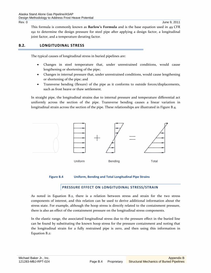
Alaska Stand Alone Gas Pipeline/ASAP Design Methodology to Address Frost Heave Potential Rev. 0 June 9, 2011
Michael Baker Jr., Inc. 121283-MBJ-RPT-024 Page B.4 Proprietary
Appendix B Structural Mechanics of Buried Pipelines
This formula is commonly known as Barlow’s Formula and is the base equation used in 49 CFR 192 to determine the design pressure for steel pipe after applying a design factor, a longitudinal joint factor, and a temperature derating factor.
B.2. LONGITUDINAL STRESS
The typical causes of longitudinal stress in buried pipelines are:
• Changes in steel temperature that, under unrestrained conditions, would cause lengthening or shortening of the pipe;
• Changes in internal pressure that, under unrestrained conditions, would cause lengthening or shortening of the pipe; and
• Transverse bending (flexure) of the pipe as it conforms to outside forces/displacements, such as frost heave or thaw settlement.
In straight pipe, the longitudinal strains due to internal pressure and temperature differential act uniformly across the section of the pipe. Transverse bending causes a linear variation in longitudinal strain across the section of the pipe. These relationships are illustrated in Figure B.4.
Figure B.4 Uniform, Bending and Total Longitudinal Pipe Strains
PRESSURE EFFECT ON LONGITUDINAL STRESS/STRAIN
As noted in Equation B.2, there is a relation between stress and strain for the two stress components of interest, and this relation can be used to derive additional information about the stress state. For example, although the hoop stress is directly related to the containment pressure, there is also an effect of the containment pressure on the longitudinal stress components.
In the elastic range, the associated longitudinal stress due to the pressure effect in the buried line can be found by substituting the known hoop stress for the pressure containment and noting that the longitudinal strain for a fully restrained pipe is zero, and then using this information in Equation B.2:
Uniform Bending Total

Alaska Stand Alone Gas Pipeline/ASAP Design Methodology to Address Frost Heave Potential Rev. 0 June 9, 2011
Michael Baker Jr., Inc. 121283-MBJ-RPT-024 Page B.5 Proprietary
Appendix B Structural Mechanics of Buried Pipelines
−
−=
−
−
pressureL
pressureH tpd
E σννε
21
110
By the second equation:
EtEpd pressureL−+
−=
σν2
0 ; or:
HpressureL tpd σνσ 3.02
==− Equation B.4
For aboveground, i.e., unrestrained sections of the pipe, the longitudinal strain is not zero
TEMPERATURE
For a pipeline that is free to expand, the strain caused as a result of temperature differential (change in temperature of the pipe steel from its installation temperature) is defined by:
( )itempL TT −=− αε
where:
εL-temp is the longitudinal strain due to temperature (in/in) in an unrestrained pipeline;
α is the coefficient of thermal expansion (in/in/°F);
T is the temperature for the state of interest (°F); and
Ti is the installation temperature (°F)
In aboveground segments of the pipeline, the thermal expansion and contraction is partially restrained and so produces longitudinal force and induces secondary longitudinal bending stress especially where the pipe configuration affords this partial restraint to thermal movement, such as near supports and at and near bends, and offsets. The design temperature differential is typically input into a pipe/structural analysis program in combination with other applicable loads to find the effects of these load components on aboveground segments.
A fully restrained pipeline has a net longitudinal strain of zero – i.e., it resists that tendency to
expand with an equal and opposite mechanical strain of: ( )itempL TT −−=− αε , thus producing a
total net strain of zero.
In the elastic range, the associated stress due to thermal restraint in the buried line can be found by noting that the associated hoop stress for this load is zero, and then using this information in Equation B.2:

Alaska Stand Alone Gas Pipeline/ASAP Design Methodology to Address Frost Heave Potential Rev. 0 June 9, 2011
Michael Baker Jr., Inc. 121283-MBJ-RPT-024 Page B.6 Proprietary
Appendix B Structural Mechanics of Buried Pipelines
−
−=
−−
−
tempLtempTL
tempH
E σνν
εε 0
111
By the second equation:
EtempL
tempL−
− =σ
ε ; or:
( ) ( )TTETTEE iitempLtempL −=−−== −− ααεσ Equation B.5
As can be seen from the equation, operating temperatures that are less than the installation temperature would cause a longitudinal tensile component (stress component is positive), while operating temperatures that are greater than the installation temperature would cause a longitudinal compressive component (stress component is negative).
BENDING
When an initially straight pipe is bent into a circular arc, longitudinal strains, and stresses, develop through the pipe cross-section in the plane of the bend. Below the proportional limit the longitudinal strain and stress in the extreme fibers of the pipe cross section are defined by:
Rr
bendingL±=−ε and R
ErbendingL
±=−σ
where:
εL-bending is maximum longitudinal strain due to bending (in/in);
σL-bending is maximum longitudinal stress due to bending (psi);
r is the outside radius of the pipe section (in); and
R is the longitudinal radius of the arc of bend of the pipe centerline (in).
When subjected to external forces/displacements a pipe resist via beam action. This beam action induces bending moments within the pipe section, which can be converted to stress by:
IMr
bendingL±=−σ
where:
I is moment of inertia of the pipe (in4); and
M is bending moment (in-lbf)

Alaska Stand Alone Gas Pipeline/ASAP Design Methodology to Address Frost Heave Potential Rev. 0 June 9, 2011
Michael Baker Jr., Inc. 121283-MBJ-RPT-024 Page B.7 Proprietary
Appendix B Structural Mechanics of Buried Pipelines
B.3. COMBINED STRESS
The general state of stress in a buried pipeline under a combination of loads can be determined by considering the principal stresses within the pipe. For biaxial stress conditions that exist in pipelines, the principal stresses are the hoop stress (σH) and the longitudinal stress (σL). The longitudinal stress is the summation of longitudinal stresses from temperature, pressure, and bending (σL-temp + σL-pressure + σL-bending). Longitudinal stresses from other axial forces, if present, are also included.
YIELD CRITERION
The two most commonly used yield criteria for determining effective stresses in pipelines are the maximum shear stress theory, commonly referred to as the Tresca theory, and the maximum distortion energy theory, commonly referred to as the von Mises’ theory.
(1) MAXIMUM SHEARING STRESSS THEORY
As discussed in “Mechanics of Materials” by Popov [Popov 1976], the maximum shearing stress theory is based on the observation that in a ductile material, slipping occurs during yielding along critically oriented planes. This suggests that the maximum shearing stress plays a key role in the yielding behavior. It is assumed that the material yielding depends on the maximum shearing stress so that whenever a critical value τcritical is reached, yielding commences. The value of τcritical is set equal to the shearing stress at yielding under uniaxial tension (+σy) or compression (–σy) loading:
2maxy
critical
σττ
±=≡
Hence, the maximum shearing stress is equal to ½ of the uniaxial yield stress. For biaxial stress conditions that exist in pipelines the corresponding yielding criterion is expressed as follows:
yH σσ ≤ and yL σσ ≤ and yLH σσσ ≤−
This is referred to as the Tresca yield criterion. The hexagonal Tresca yield function is illustrated in longitudinal stress vs. hoop stress space in Figure B.5 for an elastic-plastic material with a yield strength of 70 ksi. Any stress falling within the hexagon indicates that the material behaves elastically while points on the hexagon indicate that the material is yielding. This criterion is implemented under B31.8 Section 833.4 to limited combined stress for restrained pipe as:
TSkLH ⋅⋅≤−σσ
where:
k is an allowable stress multiplier (for loads of long duration, k is 0.90, and for occasional non-periodic loads of short duration it is 1.0);
S is the pipe SMYS; and
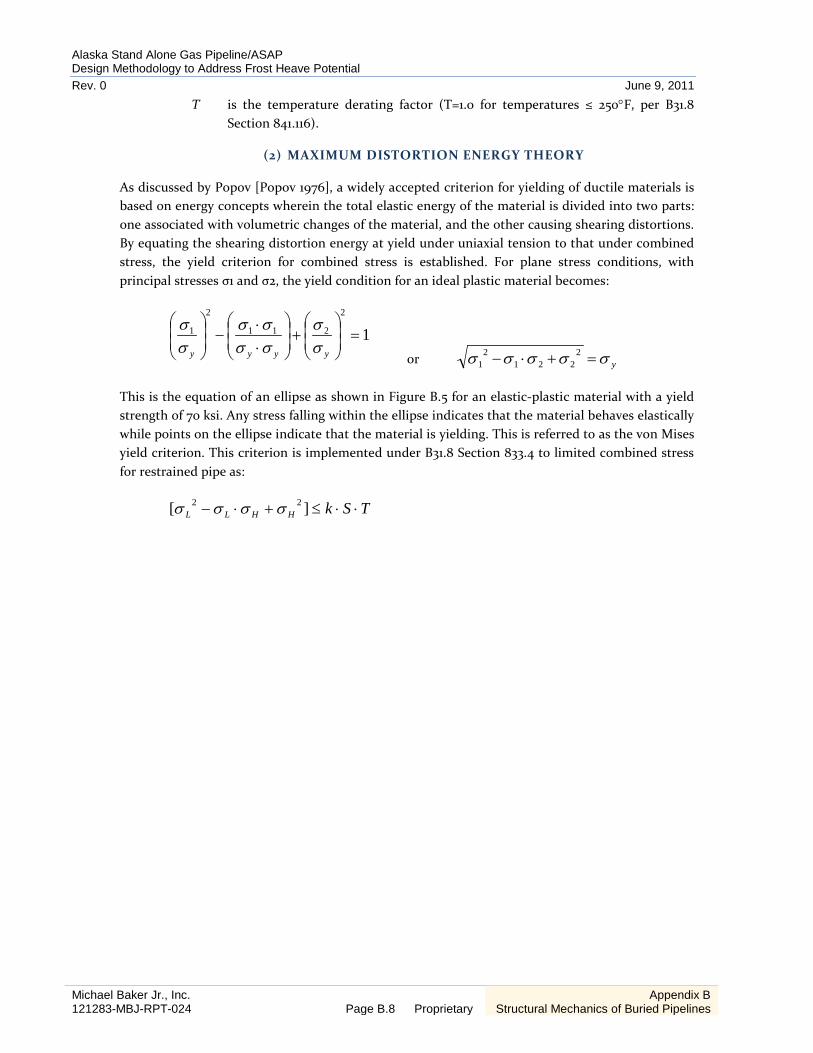
Alaska Stand Alone Gas Pipeline/ASAP Design Methodology to Address Frost Heave Potential Rev. 0 June 9, 2011
Michael Baker Jr., Inc. 121283-MBJ-RPT-024 Page B.8 Proprietary
Appendix B Structural Mechanics of Buried Pipelines
T is the temperature derating factor (T=1.0 for temperatures ≤ 250°F, per B31.8 Section 841.116).
(2) MAXIMUM DISTORTION ENERGY THEORY
As discussed by Popov [Popov 1976], a widely accepted criterion for yielding of ductile materials is based on energy concepts wherein the total elastic energy of the material is divided into two parts: one associated with volumetric changes of the material, and the other causing shearing distortions. By equating the shearing distortion energy at yield under uniaxial tension to that under combined stress, the yield criterion for combined stress is established. For plane stress conditions, with principal stresses σ1 and σ2, the yield condition for an ideal plastic material becomes:
12
211
2
1 =
+
⋅⋅
−
yyyy σσ
σσσσ
σσ
or yσσσσσ =+⋅− 2221
21
This is the equation of an ellipse as shown in Figure B.5 for an elastic-plastic material with a yield strength of 70 ksi. Any stress falling within the ellipse indicates that the material behaves elastically while points on the ellipse indicate that the material is yielding. This is referred to as the von Mises yield criterion. This criterion is implemented under B31.8 Section 833.4 to limited combined stress for restrained pipe as:
TSkHHLL ⋅⋅≤+⋅− ][ 22 σσσσ
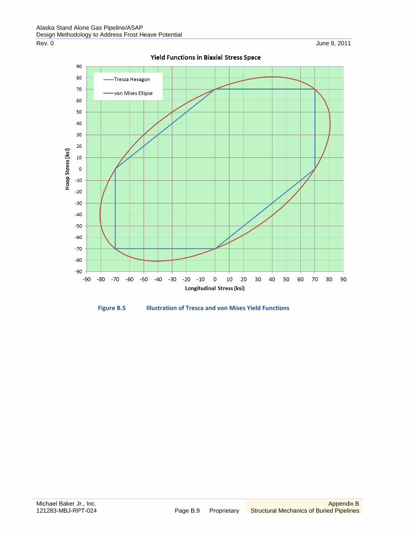
Alaska Stand Alone Gas Pipeline/ASAP Design Methodology to Address Frost Heave Potential Rev. 0 June 9, 2011
Michael Baker Jr., Inc. 121283-MBJ-RPT-024 Page B.9 Proprietary
Appendix B Structural Mechanics of Buried Pipelines
Figure B.5 Illustration of Tresca and von Mises Yield Functions