appendix d broadband over power line emission measurements d.1

D-1

APPENDIX D BROADBAND OVER POWER LINE

EMISSION MEASUREMENTS

D.1 INTRODUCTION

This appendix presents measurements performed by NTIA’s Institute for Telecommunications Sciences (ITS) that quantified several aspects of BPL signals. The measurements were conducted in three areas where BPL systems are currently deployed for testing and are serving customers. Access BPL was implemented on MV wires in all three areas and in-house BPL was implemented on LV wires in two areas. Some access BPL was on overhead wires and some is on underground wires, whereas, all of the in-house BPL was above ground except where, in some cases, there were buried LV wires leading up to the houses. The objectives for the measurements were to:

1. Measure the received BPL signal power at points along power lines; 2. Measure the received BPL signal power at various distances from power lines; 3. Measure the received BPL signal peak, average and quasi-peak levels for comparison; 4. Measure the received BPL signal power at different antenna heights; and 5. Measure the amplitude probability distributions (APDs) of the BPL signal.

The measurement system used for this testing is described in Section D.2. Figures and tables of measured data are provided in Section D.3. In section D.4 of this report, background information about APDs is covered, and in Section D.5, gain and noise figure calibration is described. D.2 THE MEASUREMENT SYSTEM The measurement system block diagram is shown in Figure D-1. An antenna, positioned 10 meters above the ground atop a telescopic mast on the ITS “RSMS-4” measurement vehicle (Figure D-2) and 2 meters above the ground on a tripod, was used to measure the received power. Four different types of antennas were used. A small discone antenna over a small ground plane was used to measure the electric fields above 30 MHz. Below 30 MHz, two shielded loops were used to measure the magnetic fields and for the electric fields, a rod antenna over a small ground plane was used. To measure the received power that is expected to be seen by a typical land mobile radio, a 2.13 meter base-loaded whip antenna was mounted on the roof of a vehicle at an approximate height of 1.5 meters. The whips were narrow-band, so several of them were used to cover the measurement frequencies. The signal from the antenna was split into two measurement systems so that simultaneous measurements could occur and to minimize switching instrument setups. A preselector was used on each system in order to prevent an overload condition from occurring and improve the sensitivity. Computers were used to control the measurement instruments and store the data.

D-2

Figure D-1: BPL measurement system block diagram.

Splitter

A n t e n n a Noise Diode

A g E4440AS p ectrumA n alyzer

H P85685P r eselector

Ag E4440ASpectrumAnalyzer

HP85685Preselector

Co m p u t e r C o m p u te r

HP8566SpectrumAnalyzer

ICO M IC-R 9 0 0 0 Rece i v e r

Ag 8 9 6 4 1 A VSA

D-3

Figure D-2: Radio Spectrum Measurement System - 4 (RSMS-4)

The output of one of the preselectors was variously connected to a HP 8566 spectrum

analyzer with a quasi-peak detector, a vector signal analyzer or a multi-mode communications receiver. The receiver was used to listen to the BPL signal in several demodulation modes and to assist with distinguishing between BPL and other signals. The vector signal analyzer was used to record the time-waveform for future analysis. D.3 BPL MEASUREMENTS D.3.1 Background on BPL Emissions Measurements

This sub-section provides general information on the BPL emissions from the three types of systems under test. These data are provided as an aid to understanding the measurements presented in Sections D.3.2 – D.3.6.

D-4

The BPL signal shown in Figure D-3 is representative of the weakest (lowest power

density) BPL signals for which data were recorded. That is, nominal interference-to-noise ratio (I/N) levels had to exceed about 5 dB; otherwise no BPL signal level (I) was recorded1. Thus, even though much weaker BPL signal levels were measurable when turning the BPL system on and off (i.e., I/N of -6 dB), measurements with I/N ≥ 5 dB ensured that measured signals were unquestionably due to BPL emissions. System #1

This system used different frequency bands for signals on the MV and LV wiring. Signal strength measurements were performed by acquiring multiple traces from a spectrum analyzer centered on specific frequencies with a zero span and a sampling detection mode. Trace data were downloaded to a computer and later analyzed statistically using Amplitude Probability Distributions (APDs). From these distributions, the temporal statistics of the BPL signal were identified and the power was determined as described in Section D.5. The signal power determined from these distributions is expressed as “100%-duty-cycle” power and represents the maximum power if the packet data were present 100% of the time (i.e. signal pulses occurring back-to-back), as further explained in Section D.4.0. System #2

The BPL signal used OFDM modulation with a carrier spacing of approximately 1.1 kHz. BPL is transmitted only on the MV lines. The downstream (towards the customer) bandwidth was 3.75 MHz while the upstream (away from the customer) bandwidth was 2.5 MHz. An example portion of the spectrum is show in Figure D-3. The BPL signal displayed a repeating pattern of three carriers, then one carrier missing, and so on. The BPL signal duty cycle was 100% for the downstream signal and between 30% - 100% for the upstream. The envelope of an upstream signal is shown in Figure D-4 and it shows a duty cycle that is in the upper end of the range.

1 If a measurement is attempted and the BPL signal has an interference to background noise level (I/N) < 5 dB, the results reported in Subsections D.3.2 – D.3.6 will be referred to as “Not measurable.” If a particular measurement isn’t attempted, it will be reported as “Not measured.” The 100% duty-cycle power levels presented in this report were analyzed statistically from APD measurements and therefore did not need to satisfy the requirement of I/N ≥ 5 dB.

D-5

Figure D-3: A portion of the System #2 BPL spectrum.

Figure D-4: The envelope of an upstream System #2 signal.

D-6

To measure System #2 emissions, the procedure involved examining the spectrum of the BPL transmission (see Figure D-3) and identifying a group of 3 adjacent carriers (since the measurement bandwidth was 3 kHz) that were among the strongest and were clear of background signals. If the signal was too weak (<5 dB above the background noise) to clearly see the spectrum or if background signals contaminated the BPL spectrum at certain frequencies, a measurement was not attempted at those frequencies. The marker in Figure D-3 shows the chosen measurement frequency. The resolution bandwidth was then set to 3 kHz and the marker (see Figure D-5) indicated the measured value using a peak detector. This value was later used to calculate the Received Power at the antenna terminals.

Figure D-5: The System #2 BPL spectrum in a 3 kHz bandwidth.

A measurement was performed to see how the received power varied as the receiver

bandwidth was changed. This is shown in Figure D-6 for a frequency of 22.957 MHz. The narrow dips in signal level are due to the signal having a duty cycle of less than 100%. The upward spikes are due to noise sources.

D-7

Figure D-6: Bandwidth progression at 22.957 MHz.

System #3

This BPL signal used DSSS modulation over the frequency range of about 1.8 to 21 MHz. BPL signals were transmitted on the MV and LV lines. The BPL signal duty cycle can be up to 90% when transmissions are occurring in both directions and about 87% for one direction. The envelope of the BPL signal is shown in Figure D-7. Four different amplitudes from four different transmitters are being received.

D-8

Figure D-7: Four different BPL transmitters.

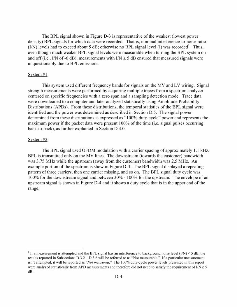
In System #3, two co-frequency BPL sources were observed transmitting at the same time, as shown in the third graticule in Figure D-8. Noise sources can be present at levels stronger than the BPL signal as shown in the eight and ninth graticules in Figure D-9.

D-9

Figure D-8: Two simultaneous BPL transmissions.

Figure D-9: Three BPL transmitters plus noise.

D-10

The measurement procedure for System #3 involved examining the spectrum of a BPL device's transmission and identifying a pair of frequencies that were the strongest and were clear of background signals. For each frequency, the signal envelope was observed for transmission bursts that were of the correct duration and pattern. Initially, the envelope was studied at a location where the BPL signals were received well. The durations of many bursts were measured to determine the typical range. This observation also yielded clearly identifiable transmission patterns that would repeat occasionally. The results of these observations were used to qualify the presence of BPL signals for future measurements. For each measurement location, the strongest BPL transmission was identified and its peak value was measured. The resolution bandwidth was then set to 30 kHz to allow for positive identification since at 3 kHz, the shorter BPL bursts would look like impulsive noise. The measured value was later used to calculate the received power at the antenna terminals. D.3.2 Measurements of BPL Along the Energized Power Line

Measurements of BPL emissions along the energized power line (Site A, Figure D-10) were made using a variety of antennas. The first measurements were taken along a fairly straight segment of power line having both a repeater and an extractor.

Figure D-10: Measurement Site A for measurements along the BPL energized power line.

Utility pole

RBPLCarrying Medium Voltage Lines

Repeater

yDevice B

Device C

To Device A

D-11

Four measurement frequencies were chosen to represent the frequency bands used by this

system (downstream injector-to-repeater, upstream repeater-to-injector, downstream repeater-to-extractor, and upstream extractor-to-repeater). Three mutually orthogonal components of the field were measured and plotted as three separate curves per graph for the frequencies 4.303, 8.125, 22.957 and 28.298 MHz, as shown in Figures D-11 through D-14 respectively. The measured peak power levels due to the orthogonal components of the electric field were plotted as a function of x, where x is the distance along the power line from the Device C. Note that in these and all other figures depicting BPL signal power vs. distance, lines connecting data points are connected to show possible trends but should not be interpreted to provide expected, interpolated values. Measurement Conditions Measurement Location: Site A Antenna Type: Rod Antenna Height: 2 meters Antenna Polarization: (X) Horizontal Parallel, (Y) Horizontal Perpendicular,

and (Z) Vertical Measured Characteristic: Peak received power due to electric field Measurement Variable: Distance along power line (x) Comments: Measurements were made at 14 positions (x-distances). At some points, the BPL signal was too weak (I/N < 5 dB), hence, some curves have fewer data points.

D-12

Figure D-11: Measured power levels along the power line – Site A, 4.303 MHz, rod antenna*


* Lines connecting data points illustrate potential trends but not expected interpolated values.

D-13




D-14

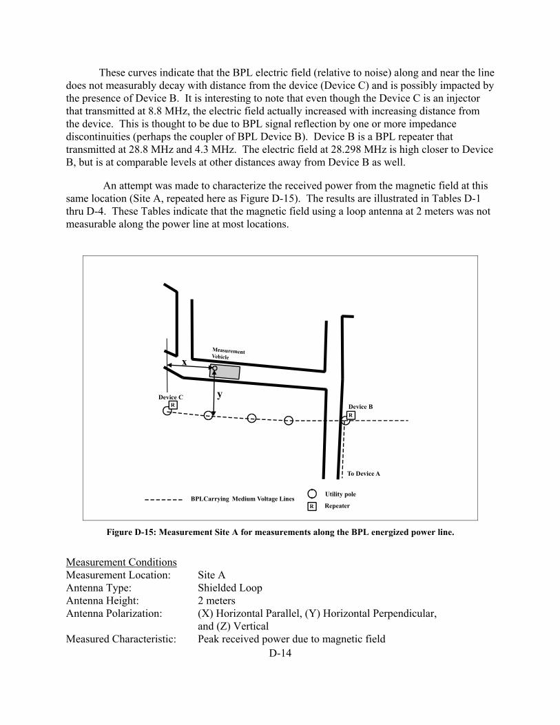
These curves indicate that the BPL electric field (relative to noise) along and near the line does not measurably decay with distance from the device (Device C) and is possibly impacted by the presence of Device B. It is interesting to note that even though the Device C is an injector that transmitted at 8.8 MHz, the electric field actually increased with increasing distance from the device. This is thought to be due to BPL signal reflection by one or more impedance discontinuities (perhaps the coupler of BPL Device B). Device B is a BPL repeater that transmitted at 28.8 MHz and 4.3 MHz. The electric field at 28.298 MHz is high closer to Device B, but is at comparable levels at other distances away from Device B as well.

An attempt was made to characterize the received power from the magnetic field at this same location (Site A, repeated here as Figure D-15). The results are illustrated in Tables D-1 thru D-4. These Tables indicate that the magnetic field using a loop antenna at 2 meters was not measurable along the power line at most locations.


Measurement Conditions Measurement Location: Site A Antenna Type: Shielded Loop Antenna Height: 2 meters Antenna Polarization: (X) Horizontal Parallel, (Y) Horizontal Perpendicular,

and (Z) Vertical Measured Characteristic: Peak received power due to magnetic field

Utility pole


Repeater

yDevice B

Device C

To Device A

D-15

Measurement Variable: Distance along power line (x) Comments: This effort was abandoned after no signal was received for many measurements.

Table D-1: Measurements along the power line – Site A, 4.303 MHz, loop antenna

X Distance (feet)

Y Distance (feet)

Received Power Z Component(dBm)

Received Power Y Component(dBm)

Received Power X Component(dBm)

648 107 Not measurable Not measurable Not measurable 612 126 Not measured Not measured Not measured 522 96 Not measured Not measured Not measured 492 93 Not measurable Not measurable Not measurable 459 87 Not measured Not measured Not measured 417 123 Not measured Not measured Not measured 357 120 Not measurable Not measurable Not measurable 309 120 Not measured Not measured Not measured 240 120 Not measured Not measured Not measured 201 120 Not measurable Not measurable Not measurable 196 120 Not measurable Not measurable Not measurable 124 120 Not measurable Not measurable Not measurable 84 135 Not measurable Not measurable Not measurable 0 120 Not measurable Not measurable Not measurable


X Distance (feet)

Y Distance (feet)




648 107 -114.94 Not measurable -114.94 612 126 Not measured Not measured Not measured 522 96 Not measured Not measured Not measured 492 93 Not measurable Not measurable Not measurable 459 87 Not measured Not measured Not measured 417 123 Not measured Not measured Not measured 357 120 Not measurable Not measurable Not measurable 309 120 Not measured Not measured Not measured 240 120 Not measured Not measured Not measured 201 120 Not measurable Not measurable Not measurable 196 120 Not measurable Not measurable Not measurable 124 120 Not measurable Not measurable Not measurable 84 135 Not measurable Not measurable Not measurable 0 120 -107.94 Not measurable Not measurable

D-16


X Distance (feet)

Y Distance (feet)




648 107 Not measurable Not measurable Not measurable 612 126 Not measured Not measured Not measured 522 96 Not measured Not measured Not measured 492 93 Not measurable Not measurable Not measurable 459 87 Not measured Not measured Not measured 417 123 Not measured Not measured Not measured 357 120 Not measurable Not measurable Not measurable 309 120 Not measured Not measured Not measured 240 120 Not measured Not measured Not measured 201 120 Not measurable Not measurable Not measurable 196 120 Not measurable Not measurable -114.33 124 120 Not measurable Not measurable Not measurable 84 135 Not measurable Not measurable Not measurable 0 120 -112.48 Not measurable -114.48


X Distance (feet)

Y Distance (feet)




648 107 -107.23 -110.23 -110.23 612 126 Not measured Not measured Not measured 522 96 Not measured Not measured Not measured 492 93 Not measurable Not measurable -112.06 459 87 Not measured Not measured Not measured 417 123 Not measured Not measured Not measured 357 120 Not measurable -112.23 Not measurable 309 120 Not measured Not measured Not measured 240 120 Not measured Not measured Not measured 201 120 -104.23 -105.23 -105.23 196 120 -111.50 Not measurable -111.50 124 120 Not measurable -112.50 -113.50 84 135 Not measurable Not measurable Not measurable 0 120 Not measurable Not measurable Not measurable

D-17

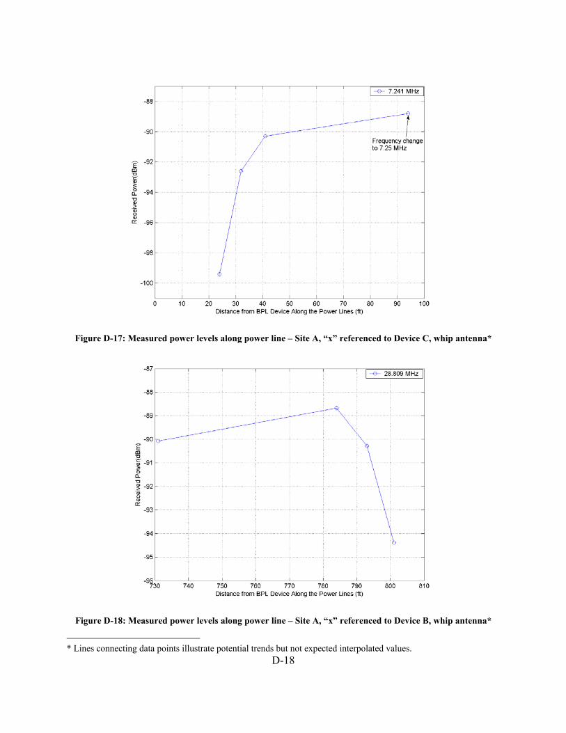
The peak received power due to the electric field was measured with the whip antenna along the power line (Site A, repeated here as Figure D-16). The measured received power levels are plotted in Figure D-17 (“x” referenced to Device C) and Figure D-18 (“x” referenced to Device B). The results are similar to those obtained from the electric field measurements previously accomplished using the rod antenna.


Measurement Conditions Measurement Location: Site A Antenna Type: Whip Antenna Height: 1.5 meters Antenna Polarization: Vertical Measured Characteristic: Peak received power due to electric field Measurement Variable: Distance along power line (x) referenced to (1) Device C, or

(2) Device B Comments: Note that though the measurements were initially made at a frequency of 7.241 MHz, the frequency was changed to 7.25 MHz due to background signals covering up the BPL signal.

Utility pole


Repeater

yDevice B

Device C

To Device A

D-18

Figure D-17: Measured power levels along power line – Site A, “x” referenced to Device C, whip antenna*

Figure D-18: Measured power levels along power line – Site A, “x” referenced to Device B, whip antenna* * Lines connecting data points illustrate potential trends but not expected interpolated values.

D-19

Measurements were taken along the BPL energized power line (Site B, Figure D-19) using a discone antenna. Figure D-20 shows a picture of the utility lines located at the intersection as viewed from the approximate location of the measurement vehicle at point C. Results are shown in Table D-5 through D-8.

Figure D-19: Measurement Site B for BPL measurements along the power line using the discone antenna.

Utility pole

Backhaul

BPL carryingmediumvoltage lines

Utility pole

Point A

Point C

x

y

Coupler

d

Mediumvoltage lines

D-20

Figure D-20: Site B power lines as viewed from the measurement vehicle located at Point C

D-21

Measurement Conditions Measurement Location: Site B Antenna Type: Discone (Model SAS-210/C) Antenna Height: 2 and 10 meters Antenna Polarization: Vertical Measured Characteristic: 100% duty cycle power (from APDs) and pulse power due to electric field Measurement Variable: Distance along power line (x) referenced to Point A, (y = 7.9 m) Comments: Measurement frequencies – 32.699 MHz and 42.465 MHz Resolution bandwidths – 30 kHz and 10 kHz Pulse power measurements – zero span, peak power detection,

2 ms sweep time (601 pts per sweep) Power lines approximately 8.5 meters above the ground

Table D-5: Measured 100%-duty-cycle power and pulse power, x = 4.9 meters (16 ft)

Ant. Ht. Frequency RBW 100%-duty-cycle Power Pulse Power Case 1 10 m 32.699 MHz 30 kHz -96.3 dBm -97.6 dBm Case 2 10 m 42.465 MHz 30 kHz Not measured -104.4 dBm Case 3 2 m 32.699 MHz 30 kHz -101.1 dBm -111.4 dBm Case 4 2 m 42.465 MHz 30 kHz Not measured -116.1 dBm Case 5 10 m 32.699 MHz 10 kHz -100.7 dBm -102.4 dBm Case 6 10 m 42.465 MHz 10 kHz Not measured -112.0 dBm Case 7 2 m 32.699 MHz 10 kHz -111.4 dBm -117.5 dBm Case 8 2 m 42.465 MHz 10 kHz Not measured -120.2 dBm


Ant. Ht. Frequency RBW 100%-duty-cycle Power Pulse Power Case 1 10 m 32.699 MHz 30 kHz Not measured -112.4 dBm Case 2 10 m 42.465 MHz 30 kHz Not measured Not measurable Case 5 10 m 32.699 MHz 10 kHz -110.1 dBm -115.2 dBm Case 6 10 m 42.465 MHz 10 kHz Not measured Not measurable


Ant. Ht. Frequency RBW 100%-duty-cycle Power Pulse Power Case 1 10 m 32.699 MHz 30 kHz -110.5 dBm -108.6 dBm Case 2 10 m 42.465 MHz 30 kHz Not measured -107.7 dBm Case 3 2 m 32.699 MHz 30 kHz Not measurable Not measurable Case 4 2 m 42.465 MHz 30 kHz Not measurable Not measurable Case 5 10 m 32.699 MHz 10 kHz -110.5 dBm -114.9 dBm Case 6 10 m 42.465 MHz 10 kHz Not measured -119.3 dBm Case 7 2 m 32.699 MHz 10 kHz Not measurable Not measurable Case 8 2 m 42.465 MHz 10 kHz Not measurable Not measurable

D-22


Ant. Ht. Frequency RBW 100%-duty-cycle Power Pulse Power Case 1 10 m 32.699 MHz 30 kHz Not measured -110.1 dBm Case 2 10 m 42.465 MHz 30 kHz -106.9 dBm -105.4 dBm Case 3 2 m 32.699 MHz 30 kHz Not measurable Not measurable Case 4 2 m 42.465 MHz 30 kHz Not measurable Not measurable Case 5 10 m 32.699 MHz 10 kHz Not measured -114.4 dBm Case 6 10 m 42.465 MHz 10 kHz -111.0 dBm -110.9 dBm Case 7 2 m 32.699 MHz 10 kHz Not measurable Not measurable Case 8 2 m 42.465 MHz 10 kHz Not measurable Not measurable

Figure D-21 summarizes the measured received power along the power lines using data

from Table D-5 through Table D-8 for a frequency of 32.699 MHz and for a vertically polarized Discone antenna at a height of 10 meters. This figure indicates that after an initial decrease of received power, the power remains at about the same level along the power line away from a Backhaul point.

Figure D-21: Measured power levels along power line – Site B, discone antenna, antenna height = 10 m, frequency = 32.699 MHz, data from Table D.3.2-5 through Table D.3.2-8*


D-23

D.3.3 Measurements of BPL Away From the Energized Power Line

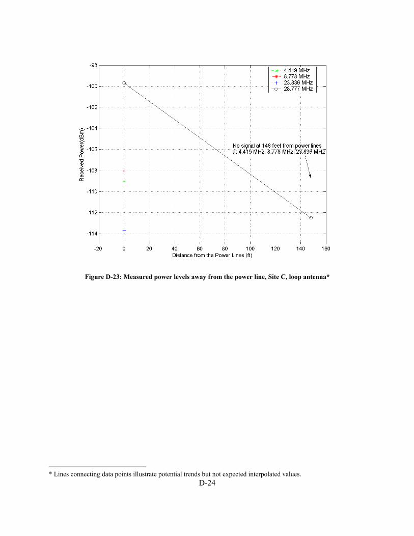
A number of measurements of BPL emissions were made with varying distance away from the power line. In general, the measurements started out close to a pole mounted BPL device and moved away until the signal level was too low to make a confident measurement. For the first measurements away from the power line, Site C’s physical layout of power lines and BPL devices is illustrated in Figure D-22 and the measured power away from the power lines is plotted in Figure D-23. With a loop antenna directly under the power line at a height of 2 meters, a small signal power was measured on all four frequencies (4.419 MHz, 8.777 MHz, 23.836 MHz and 28.777 MHz). At a distance of 148 feet from the power line, the signal was received only at 28.777 MHz as shown in Figure D-23.

Figure D-22: Measurement Site C for BPL measurements away from the power line at Device B Measurement Conditions Measurement Location: Site C Antenna Type: Shielded Loop Antenna Height: 2 meters Antenna Polarization: Horizontal Parallel Measured Characteristic: Peak received power due to magnetic field Measurement Variable: Distance away from power line (x) Comments: Device A is an Extractor transmitting an upstream signal at 23.8 MHz. Device B is a repeater transmitting on 28.8 MHz downstream and 4.4 MHz upstream. Device C is an injector transmitting on 8.8 MHz downstream. When the antenna was moved 45.1 meters (148 ft) away from the power line the signal was not received on 3 of the 4 frequencies.

Utility pole


Repeater

Device BDevice C

To Device A

D-24

Figure D-23: Measured power levels away from the power line, Site C, loop antenna*


D-25

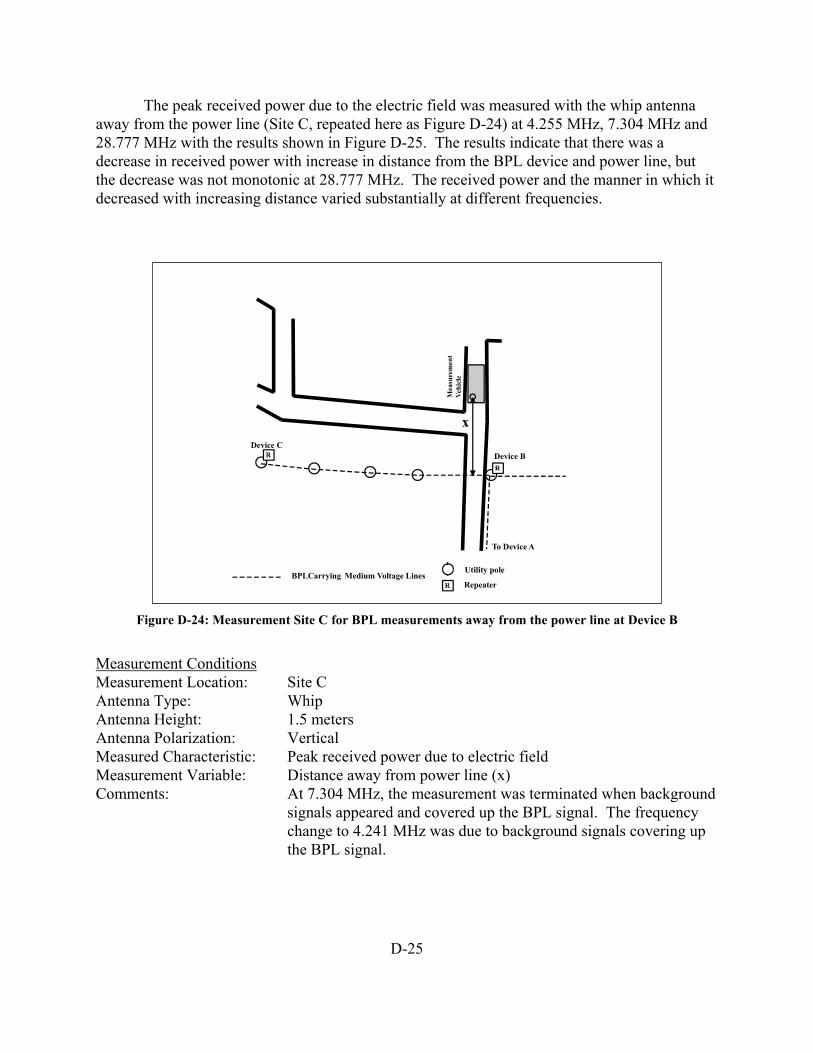
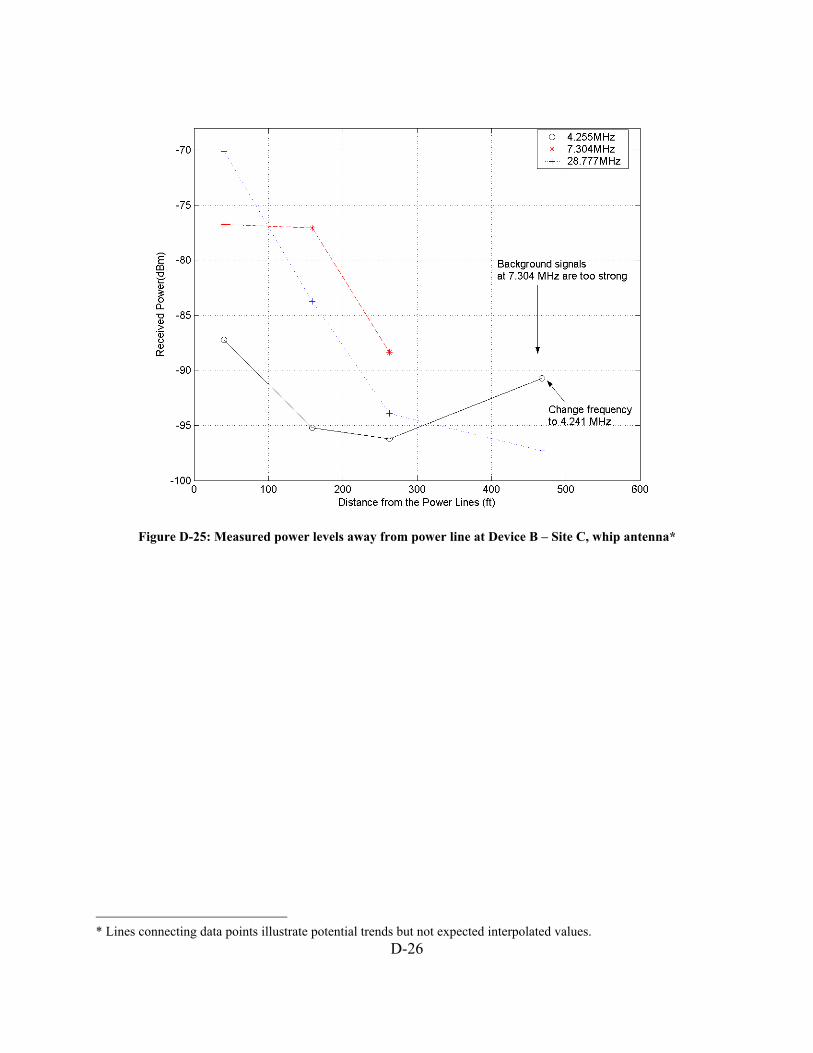
The peak received power due to the electric field was measured with the whip antenna away from the power line (Site C, repeated here as Figure D-24) at 4.255 MHz, 7.304 MHz and 28.777 MHz with the results shown in Figure D-25. The results indicate that there was a decrease in received power with increase in distance from the BPL device and power line, but the decrease was not monotonic at 28.777 MHz. The received power and the manner in which it decreased with increasing distance varied substantially at different frequencies.

Figure D-24: Measurement Site C for BPL measurements away from the power line at Device B

Measurement Conditions Measurement Location: Site C Antenna Type: Whip Antenna Height: 1.5 meters Antenna Polarization: Vertical Measured Characteristic: Peak received power due to electric field Measurement Variable: Distance away from power line (x) Comments: At 7.304 MHz, the measurement was terminated when background signals appeared and covered up the BPL signal. The frequency change to 4.241 MHz was due to background signals covering up the BPL signal.

Utility pole


Repeater

Device BDevice C

To Device A

D-26

Figure D-25: Measured power levels away from power line at Device B – Site C, whip antenna*


D-27

The peak received power due to the electric field was measured with the whip antenna on a different path (measurement trend line) as a function of distance from the power line as shown in Figure D-26. The results, plotted in Figure D-27, show that even though the received power generally decreased with distance from Device C, the peak power level at 28.809 MHz exhibited significant oscillations as a function of increasing distance.

Figure D-26: Measurement Site C for BPL measurements away from the power line at Device C Measurement Conditions Measurement Location: Site C Antenna Type: Whip Antenna Height: 1.5 meters Antenna Polarization: Vertical Measured Characteristic: Peak received power due to electric field Measurement Variable: Distance away from power line (x) Comments: At 7.241 MHz, the measurement was terminated when background signals appeared and covered up the BPL signal.

Utility pole


Repeater

Device BDevice C

To Device A

D-28

Figure D-27: Measured power levels away from power line at Device B – Site C, whip antenna*


D-29

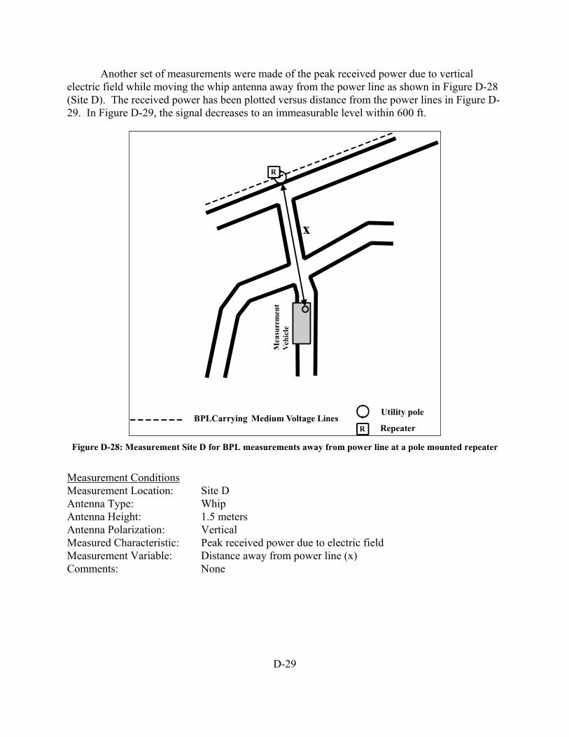
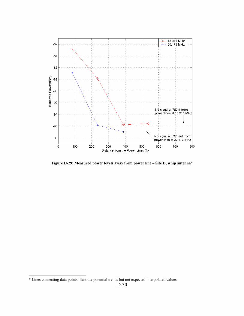
Another set of measurements were made of the peak received power due to vertical electric field while moving the whip antenna away from the power line as shown in Figure D-28 (Site D). The received power has been plotted versus distance from the power lines in Figure D-29. In Figure D-29, the signal decreases to an immeasurable level within 600 ft.

Figure D-28: Measurement Site D for BPL measurements away from power line at a pole mounted repeater Measurement Conditions Measurement Location: Site D Antenna Type: Whip Antenna Height: 1.5 meters Antenna Polarization: Vertical Measured Characteristic: Peak received power due to electric field Measurement Variable: Distance away from power line (x) Comments: None

Utility pole


Repeater

D-30

Figure D-29: Measured power levels away from power line – Site D, whip antenna*


D-31

The next measurements were made away from the power lines at Site E. The physical layout (Figure D-30) shows several repeaters and one concentrator (injector) and a network of MV lines all transmitting at various times over the same frequency range. In Figure D-31, the received power at 8.1 MHz and 14.8 MHz are plotted versus distance from the power lines, out to a distance exceeding 1500 ft, where the BPL signal diminished to within 5 dB of the noise floor.

Figure D-30: Measurement Site E for BPL measurements away from power line at a repeater Measurement Conditions Measurement Location: Site E Antenna Type: Whip Antenna Height: 1.5 meters Antenna Polarization: Vertical Measured Characteristic: Peak received power due to electric field Measurement Variable: Distance away from power line (x) Comments: None

Utility pole

x

R

R

R R

R

R

R

R

R

R

R

R

C

C

BPL 1-Phase MV Lines

BPL 3-Phase MV Lines

Concentrator

Repeater

D-32

Figure D-31: Measured power levels away from power line – Site E, whip antenna*


D-33

The peak received power was measured using both whip and loop antennas at heights of 1.5 and 2 meters, respectively, near a transformer with underground power lines (Site F) carrying BPL signals. The measurements show that at 6.4 meters (21 ft) from the transformer, the BPL signal power was measurable at one of the three BPL frequencies as shown in Table D-9. At 29.3 meters (96 ft) from the transformer, no signal could be detected. Measurement Conditions Measurement Location: Site F Antenna Type: Whip, Shielded Loop Antenna Height: 1.5 meters (whip) and 2 meters (loop) Antenna Polarization: Whip - Vertical, Loop - Vertical Parallel, Vertical Perpendicular

and Horizontal Measured Characteristic: Peak received power due to electric and magnetic fields Measurement Variable: Distance away from power line (x) Comments: None

Table D-9: Measure power levels away from power line – Site F, whip & loop antennas

Measurement Distance

Frequency (MHz)

Whip (Vertical)

Loop (Vertical, parallel to the power

line)

Loop (Vertical,

perpendicular to the power

line)

Loop (Horizontal)

6.4 m (21 ft) 3.99 Not measurable

Not measurable

Not measurable

Not measurable


Not measurable

Not measurable

Not measurable

6.4 m (21 ft) 15.285 -80 dBm -114 dBm Not measurable -114 dBm


Not measurable

Not measurable

Not measurable


Not measurable

Not measurable

Not measurable


Not measurable

Not measurable

Not measurable

D-34

Measurements were performed using a discone antenna with the power line configuration as shown in Figure D-32 for Site G. Manual pulse power measurements are plotted for three frequencies, 35.04992 MHz, 39.92954 MHz and 45.40195 MHz, as shown in Figure D-33. Also included are theoretical plots for loss proportional to 1/R, 1/R2, and 1/R4, where “R” is distance from the power line (i.e., “R” is depicted as the parameter “x” in Figure D-32). The results indicate that the received power decreases as distance from the power line increases at a rate lower than would be predicted by 1/R2 (space wave loss).

Figure D-32: Measurement Site G for BPL measurements away from power line using the discone antenna

Measurement Conditions Measurement Location: Site G Antenna Type: Discone (Model SAS-210/C) Antenna Height: 3.4 meters (11.2 ft) Antenna Polarization: Vertical Measured Characteristic: Peak received power due to electric field Measurement Variable: Distance away from power line (x) Comments: Measurement frequencies – 35.04492 MHz, 39.92954 MHz, and 45.40195 MHz Resolution bandwidths – 200 kHz Pulse power measurements – zero span, peak power detection,


Utility pole

Street B

x

Backhaul


y

D-35

Figure D-33: Received pulse power measured away from power line – Site G, discone antenna*


D-36

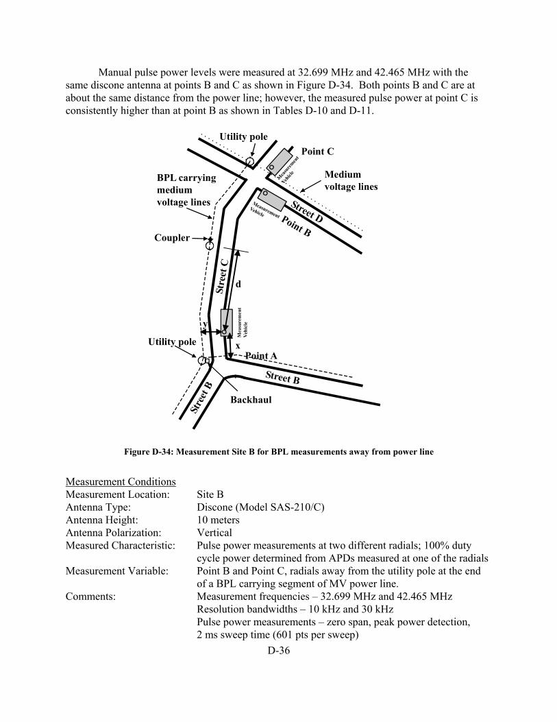
Manual pulse power levels were measured at 32.699 MHz and 42.465 MHz with the same discone antenna at points B and C as shown in Figure D-34. Both points B and C are at about the same distance from the power line; however, the measured pulse power at point C is consistently higher than at point B as shown in Tables D-10 and D-11.

Figure D-34: Measurement Site B for BPL measurements away from power line

Measurement Conditions Measurement Location: Site B Antenna Type: Discone (Model SAS-210/C) Antenna Height: 10 meters Antenna Polarization: Vertical Measured Characteristic: Pulse power measurements at two different radials; 100% duty

cycle power determined from APDs measured at one of the radials Measurement Variable: Point B and Point C, radials away from the utility pole at the end

of a BPL carrying segment of MV power line. Comments: Measurement frequencies – 32.699 MHz and 42.465 MHz Resolution bandwidths – 10 kHz and 30 kHz Pulse power measurements – zero span, peak power detection,

2 ms sweep time (601 pts per sweep)

Utility pole

Backhaul


Utility pole

Point A

Point C

x

y

Coupler

d

Mediumvoltage lines

D-37

Table D-10: Measured pulse power – Site B, Point B, discone antenna, radial 20.7 meters from utility pole.

Frequency RBW Pulse Power Case 1 32.699 MHz 30 kHz Not measurable Case 2 42.465 MHz 30 kHz -112.2 dBm Case 3 32.699 MHz 10 kHz Not measurable Case 4 42.465 MHz 10 kHz Not measurable

Table D-11: Measured 100%-duty-cycle power and pulse power – Site B, Point C, discone antenna, radial

20.4 meters from utility pole.

Frequency RBW 100%-duty-cycle Power

Pulse Power

Case 1 32.699 MHz 30 kHz -104.1 dBm -106.4 dBm Case 2 42.465 MHz 30 kHz Not measured -110.2 dBm Case 3 32.699 MHz 10 kHz -109.7 dBm -109.7 dBm Case 4 42.465 MHz 10 kHz Not measured Not measurable

D.3.4 Measurements of BPL Using Various Detectors

Measurements were made using three different spectrum analyzer detectors (peak, average and quasi-peak.) at Site A, as shown in Figure D-35. Table D-12 and D-13 show the detector levels for the two measurement frequencies. The data shown in these tables indicate that the measured quasi-peak power levels for this BPL signal are 0 to 5 dB greater than the average power levels.

D-38

Figure D-35: Measurement Site A for BPL measurements using various detectors

Measurement Conditions Measurement Location: Site A Antenna Type: Whip Antenna Height: 1.5 meters Antenna Polarization: Vertical Measured Characteristic: Peak, average, and quasi-peak power due to electric field Measurement Variable: Distance away from power line (x, y) Comments: Resolution bandwidths – 9.1 kHz (peak & average),

9 kHz quasi-peak Signal-to-noise ratio (SNR) at 22.957 MHz was 8 dB SNR at 28.298 MHz was 38 dB.

Table D-12: Measured peak, average and quasi-peak levels, x = 150 m, y = 28.3 m

Detector Peak Average Quasi-Peak Value at f = 22.957 MHz -74 dBm -81 dBm -76 dBm

Utility pole


Repeater

yDevice B

Device C

To Device A

D-39

Table D-13: Measured peak, average and quasi-peak levels, x = 58.2 m, y = 39.3 m

Detector Peak Average Quasi-Peak Value at f = 28.298 MHz -60 dBm -65 dBm -65 dBm

The measurements using the various detectors were made in a residential neighborhood environment. There were noise sources present, some of them appear impulsive on a spectrum analyzer and some appear bursty. Figure D-36 shows both kinds of noise sources at levels higher than the BPL signal. While it is possible to read the BPL level in between these noise sources with a peak and average (due to the 100% BPL duty cycle and if the symbol period is short enough) detector, the quasi-peak detector, with its longer time constant, will include the noise power in its measurement. When the BPL signal has a duty cycle less than 100% with a period greater than the period of the noise sources, the average detector will include the noise power in its measurement. An example of this signal is shown in Figure D-37. The period of the noise sources is much shorter than the period of the BPL signal. The off periods are large enough to cause the quasi-peak detector level to decay, Figure D-38, so to obtain a single value the operator chose a value when the BPL signal was on and ignored the noise induced spike near the center of the trace.

Figure D-36: BPL signal at 28.298 MHz.

D-40



D-41

Another measurement was made to compare detectors at a different location at Site A and on a different day. The results are in Table D-14. Measurement Conditions Measurement Location: Site A Antenna Type: Whip Antenna Height: 1.5 meters Antenna Polarization: Vertical Measured Characteristic: Peak, average, and quasi-peak power due to electric field Measurement Variable: Distance away from power line (x, y) Comments: Resolution bandwidths – 3 kHz , corresponding to a typical

land-mobile signal bandwidth in the HF spectrum

Table D-14: Measured detector levels, x – directly in front of Device B, y = 12.2 m

Frequency Detector 4.255 MHz 7.304 MHz 28.777 MHz Peak -72 dBm -60.4 dBm -54.8 dBm Average -74.8 dBm -63.5 dBm -56.6 dBm Quasi-Peak -71.3 dBm -59.3 dBm -55.3 dBm

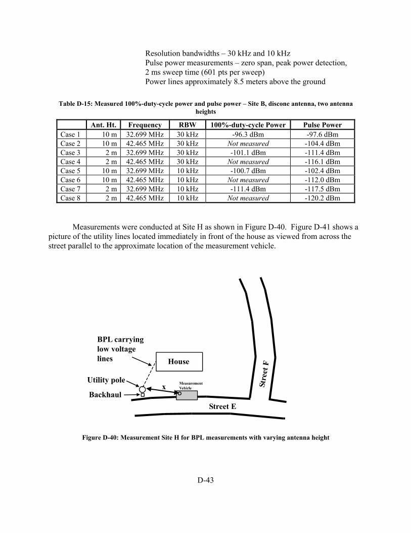
D.3.5 Measurements of BPL Varying Antenna Height

Measurements were performed using two different antenna heights at Site B, Figure D-39. Results are shown in Table D-15. The results show that in general, the measured power levels were higher at the greater antenna height. For example, the 100% duty cycle power measured at a frequency of 32.699 MHz and at a 10 meter antenna height was 4.8 to 10.7 dB greater than at 2 meters. The pulse power at a 10 meter antenna height for this same frequency was 8.2 to 15.1 dB higher than at 2 meters.

D-42

Figure D-39: Measurement Site B for BPL measurements with varying antenna height Measurement Conditions Measurement Location: Site B Antenna Type: Discone (Model SAS-210/C) Antenna Height: 2 and 10 meters Antenna Polarization: Vertical Measured Characteristic: 100% duty cycle power (from APDs) and pulse power due to electric field Measurement Variable: Distance along power line (x = 4.9 m) referenced to Point A, (y =

7.9 m) Comments: Measurement frequencies – 32.699 MHz and 42.465 MHz

Utility pole

Backhaul


Utility pole

Point A

Point C

x

y

Coupler

d

Mediumvoltage lines

D-43

Resolution bandwidths – 30 kHz and 10 kHz Pulse power measurements – zero span, peak power detection,


Table D-15: Measured 100%-duty-cycle power and pulse power – Site B, discone antenna, two antenna

heights

Ant. Ht. Frequency RBW 100%-duty-cycle Power Pulse Power Case 1 10 m 32.699 MHz 30 kHz -96.3 dBm -97.6 dBm Case 2 10 m 42.465 MHz 30 kHz Not measured -104.4 dBm Case 3 2 m 32.699 MHz 30 kHz -101.1 dBm -111.4 dBm Case 4 2 m 42.465 MHz 30 kHz Not measured -116.1 dBm Case 5 10 m 32.699 MHz 10 kHz -100.7 dBm -102.4 dBm Case 6 10 m 42.465 MHz 10 kHz Not measured -112.0 dBm Case 7 2 m 32.699 MHz 10 kHz -111.4 dBm -117.5 dBm Case 8 2 m 42.465 MHz 10 kHz Not measured -120.2 dBm

Measurements were conducted at Site H as shown in Figure D-40. Figure D-41 shows a picture of the utility lines located immediately in front of the house as viewed from across the street parallel to the approximate location of the measurement vehicle.

Figure D-40: Measurement Site H for BPL measurements with varying antenna height

Utility pole

Backhaul

BPL carryinglow voltagelines

x

Street E

House

D-44

Measurement Conditions Measurement Location: Site H Antenna Type: Shielded Loop Antenna Height: 2 meters and 10 meters Antenna Polarization: Vertical, plane of antenna perpendicular to power line Measured Characteristic: Pulse power measurements and 100% duty cycle power (from

APDs) of the magnetic field Measurement Variable: Distance away from low voltage power line (x = 8.7 meters) Comments: Measurement frequencies – 5.00 MHz, 6.43 MHz, 10.74 MHz

and 18.38 MHz Resolution bandwidths – 3 kHz and 10 kHz Pulse power measurements – zero span, peak power detection,

5 ms sweep time (601 pts per sweep) Power line height ranging approximately 3 – 4.3 meters

The pulse-power and the 100%-duty-cycle power (both referenced to the antenna output)

are shown for each case in Table D-16. The results shown indicate that measured power at a 10 meter height was always larger than the power measured at 2 meter height (by 3-10 dBm).

D-45

Backhaul

Low voltageline to house

Coupler

Figure D-41: Measurement Site H utility lines located immediately in front of house as viewed from

across the street parallel to the approximate location of the measurement vehicle.

D-46

Table D-16: Measured 100%-duty-cycle power and pulse power – Site H, loop antenna, two antenna heights

Ant. Ht.

Frequency RBW 100%-duty-cycle Power

Pulse Power

Case 1 10 m 5.00 MHz 10 kHz Not measurable Not measurableCase 2 10 m 5.00 MHz 3 kHz Not measurable Not measurableCase 3 10 m 6.43 MHz 10 kHz -106.4 dBm -112.3 dBmCase 4 10 m 6.43 MHz 3 kHz -108.7 dBm -114.0 dBmCase 5 10 m 10.74 MHz 10 kHz Not measured -110.3 dBmCase 6 10 m 10.74 MHz 3 kHz -114.8 dBm Not measurableCase 7 10 m 18.38 MHz 10 kHz Not measured -101.4 dBmCase 8 10 m 18.38 MHz 3 kHz -106.6 dBm -110.8 dBmCase 9 2 m 5.00 MHz 10 kHz Not measurable Not measurableCase 10 2 m 5.00 MHz 3 kHz Not measurable Not measurableCase 11 2 m 6.43 MHz 10 kHz -109.1 dBm Not measurableCase 12 2 m 6.43 MHz 3 kHz -113.3 dBm -112.6 dBmCase 13 2 m 10.74 MHz 10 kHz Not measurable Not measurableCase 14 2 m 10.74 MHz 3 kHz Not measurable Not measurableCase 15 2 m 18.38 MHz 10 kHz -111.2 dBm -113.3 dBmCase 16 2 m 18.38 MHz 3 kHz -115.3 dBm -117.3 dBm

D-47

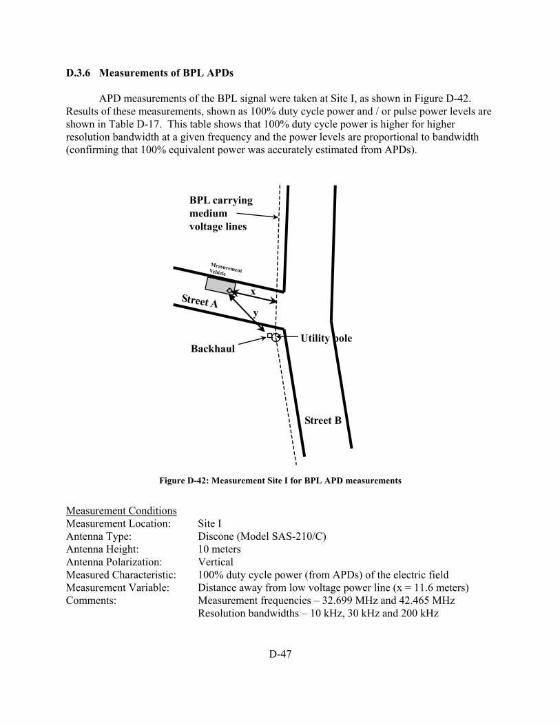
D.3.6 Measurements of BPL APDs

APD measurements of the BPL signal were taken at Site I, as shown in Figure D-42. Results of these measurements, shown as 100% duty cycle power and / or pulse power levels are shown in Table D-17. This table shows that 100% duty cycle power is higher for higher resolution bandwidth at a given frequency and the power levels are proportional to bandwidth (confirming that 100% equivalent power was accurately estimated from APDs).

Figure D-42: Measurement Site I for BPL APD measurements Measurement Conditions Measurement Location: Site I Antenna Type: Discone (Model SAS-210/C) Antenna Height: 10 meters Antenna Polarization: Vertical Measured Characteristic: 100% duty cycle power (from APDs) of the electric field Measurement Variable: Distance away from low voltage power line (x = 11.6 meters) Comments: Measurement frequencies – 32.699 MHz and 42.465 MHz Resolution bandwidths – 10 kHz, 30 kHz and 200 kHz

Utility pole

Street B

x

Backhaul


y

D-48

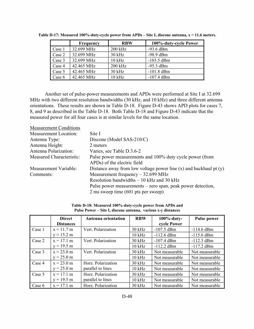
Table D-17: Measured 100%-duty-cycle power from APDs – Site I, discone antenna, x = 11.6 meters.

Frequency RBW 100%-duty-cycle Power Case 1 32.699 MHz 200 kHz -93.6 dBm Case 2 32.699 MHz 30 kHz -98.9 dBm Case 3 32.699 MHz 10 kHz -103.5 dBm Case 4 42.465 MHz 200 kHz -95.3 dBm Case 5 42.465 MHz 30 kHz -101.8 dBm Case 6 42.465 MHz 10 kHz -107.4 dBm

Another set of pulse-power measurements and APDs were performed at Site I at 32.699 MHz with two different resolution bandwidths (30 kHz, and 10 kHz) and three different antenna orientations. These results are shown in Table D-18. Figure D-43 shows APD plots for cases 7, 8, and 9 as described in the Table D-18. Both Table D-18 and Figure D-43 indicate that the measured power for all four cases is at similar levels for the same location. . Measurement Conditions Measurement Location: Site I Antenna Type: Discone (Model SAS-210/C) Antenna Height: 2 meters Antenna Polarization: Varies, see Table D.3.6-2 Measured Characteristic: Pulse power measurements and 100% duty cycle power (from

APDs) of the electric field Measurement Variable: Distance away from low voltage power line (x) and backhaul pt (y) Comments: Measurement frequency – 32.699 MHz Resolution bandwidths – 10 kHz and 30 kHz Pulse power measurements – zero span, peak power detection,

2 ms sweep time (601 pts per sweep)

Table D-18: Measured 100%-duty-cycle power from APDs and Pulse Power – Site I, discone antenna, various x-y distances

Direct Distances

Antenna orientation RBW 100%-duty-cycle Power

Pulse power

30 kHz -107.5 dBm -114.6 dBm Case 1 x = 11.7 m y = 15.2 m

Vert. Polarization 10 kHz -112.6 dBm -115.6 dBm 30 kHz -107.4 dBm -112.3 dBm Case 2 x = 17.1 m

y = 19.5 m Vert. Polarization

10 kHz -112.2 dBm -117.2 dBm 30 kHz Not measurable Not measurable Case 3 x = 23.0 m

y = 25.0 m Vert. Polarization

10 kHz Not measurable Not measurable 30 kHz Not measurable Not measurable Case 4 x = 23.0 m

y = 25.0 m Horz. Polarization parallel to lines 10 kHz Not measurable Not measurable

30 kHz Not measurable Not measurable Case 5 x = 17.1 m y = 19.5 m

Horz. Polarization parallel to lines 10 kHz Not measurable Not measurable

Case 6 x = 17.1 m Horz. Polarization 30 kHz Not measurable Not measurable

D-49

y = 19.5 m perpendicular to lines 10 kHz Not measurable Not measurable 30 kHz -107.9 dBm -110.1 dBm Case 7 x = 11.7 m

y = 15.2 m Horz. Polarization perpendicular to lines 10 kHz -113.1 dBm -115.8 dBm


Horz. Polarization parallel to lines 10 kHz -113.3 dBm -118.1 dBm


Horz. Polarization pointed to pole 10 kHz -109.0 dBm -116.8 dBm

The 100% duty-cycle power and manual pulse power levels were observed to be nearly the same for measurements performed at the same location with the antenna pointed in different directions (Case 7 – Case 9).

Figure D-43: APD measurements in a 30 kHz RBW for three different antenna

orientations – Site I, located with a 11.7 m direct distance from power lines

D-50

D.4 BACKGROUND ON AMPLITUDE PROBABILITY DISTRIBUTIONS

Because of the random nature of the system noise, background noise, and the BPL signal itself, signal power data were, at times, collected and analyzed statistically using amplitude probability distributions (APDs).2

The reason for using APDs was to differentiate the BPL signal from the background (and system) noise and to extract mean power. While the APD can be used to characterize the background noise, doing so requires a sufficiently large ensemble and adequate sensitivity. It was not the original intention to use these measurements for the purpose of characterizing the background noise; therefore, the extent of sampling and the system configuration limit the use of these APDs for that purpose.

Data for these measurements were acquired by repeatedly collecting power traces from a spectrum analyzer and placing the power values in corresponding 0.1-dB bins of a histogram (later to be used for creating APDs). The spectrum analyzer was set in sample detection mode with a zero span and centered on specified frequencies of interest. So as to assure uncorrelated sampling, the trace sweep-time was set so that adjacent data points were no closer in time than 2/RBW, where RBW is the resolution bandwidth. To provide sufficient probability resolution, a minimum of 500,000 samples were collected for each APD - enough to give a probability of a single occurrence equal to 0.0002% .

By repeatedly collecting power data when the transmission lines are loaded with BPL and when the BPL is turned off, it is possible to identify the power contribution by BPL, assuming that the background noise does not change significantly. For example, Figure D-44 shows the APDs for the two scenarios - BPL on and BPL off. The “system noise” plot is emulated by calculating the curve from the system noise figure. Though the data from the two scenarios were not collected simultaneously, the characteristics of the noise environment, in this case, were changed only by inclusion or exclusion of the BPL signal. The features noted between points B and D are due predominantly to the BPL signal, whereas the features between points A and B for the “BPL-loaded” case and points A and C for the “BPL-off” case are due predominantly to extraneous environmental impulsive noise. The linear regions of the curves are due to system noise.

By taking multiple APDs of these two scenarios, it is possible to identify APD features that are characteristic of the BPL signal. For instance, after examining multiple APDs, it was possible to conclude that, for this example data, the BPL signal is present approximately 10% of the time when loaded. Figure D-45 shows data collected in a slightly different location within the site. However, in this example, changes in the noise environment between “loaded” and “off” cases are due not only to the BPL being turned off, but also due to some additional impulsive noise as noted in the region between points B and D of the “BPL-off” plot. Despite 2 “Measurements to determine potential interference to GPS receivers from ultrawideband transmission systems,” J.R. Hoffman, M.G. Cotton, R.J. Achatz, R.N. Statz, and R.A. Dalke, NTIA Report 01-384, Feb. 2001.

D-51

this added complexity, it is still possible to identify the power contribution by BPL because the region between points C and E on the “BPL-loaded” plot has the characteristic feature of 10% presence, and this feature of the curve is absent for the “BPL-off” case.

Figure D-44: Example APD plots for two different measurement scenarios - BPL loaded and BPL off.

Figure D-45: Example APD plots for two different measurement scenarios - BPL loaded and BPL off.

D-52

For each of the APD plots, the powers on the ordinate are referenced to the output of the

antenna terminals. Mean powers are calculated from the associated histograms by: where xi is power in the ith bin, ni is the number of samples in the ith bin, and N is the total number of samples. In cases where the system noise or environmental noise may contribute significantly to the overall signal power, the mean signal power of the BPL is determined by subtracting the mean system noise power and/or environmental noise from the overall mean signal power. In some cases, the background noise is low enough in power or infrequent enough (for impulsive noise) that their contribution to the overall power can be disregarded.

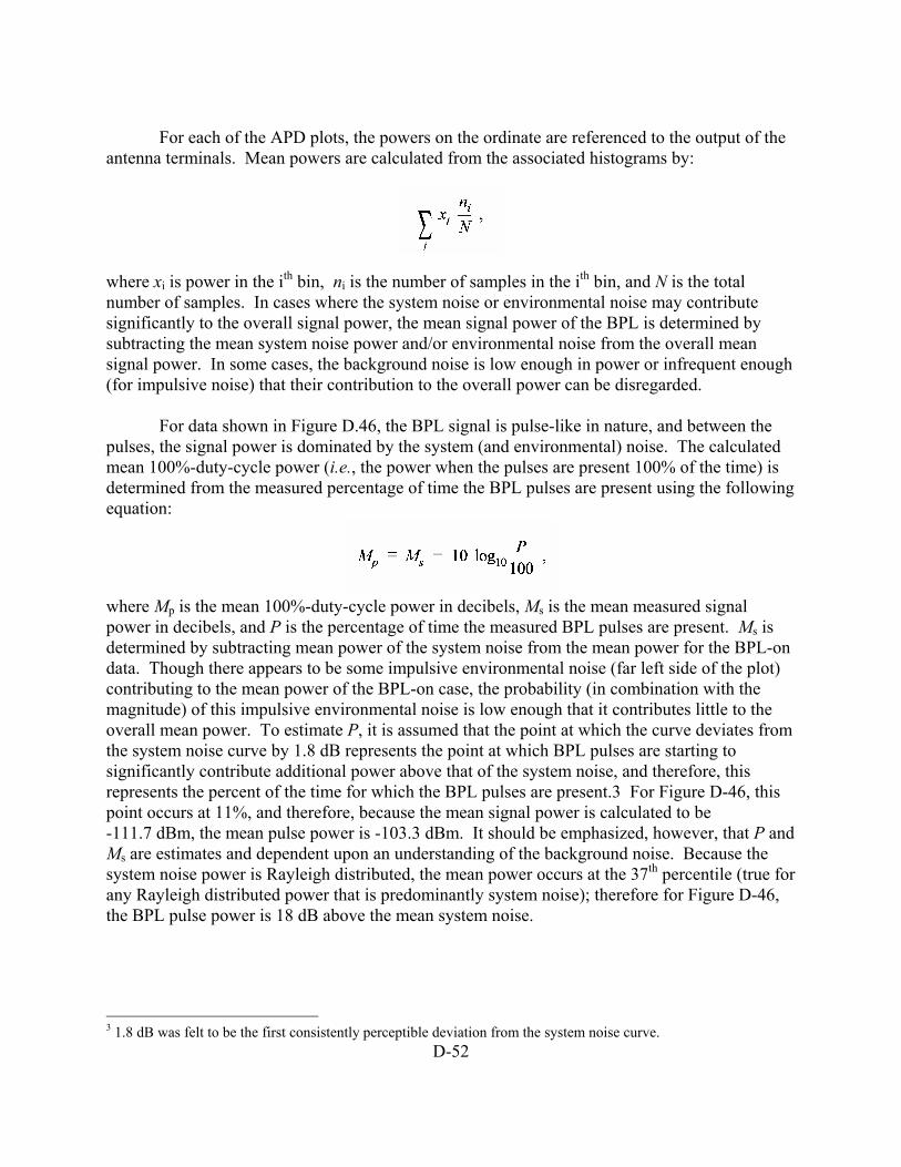
For data shown in Figure D.46, the BPL signal is pulse-like in nature, and between the pulses, the signal power is dominated by the system (and environmental) noise. The calculated mean 100%-duty-cycle power (i.e., the power when the pulses are present 100% of the time) is determined from the measured percentage of time the BPL pulses are present using the following equation:

where Mp is the mean 100%-duty-cycle power in decibels, Ms is the mean measured signal power in decibels, and P is the percentage of time the measured BPL pulses are present. Ms is determined by subtracting mean power of the system noise from the mean power for the BPL-on data. Though there appears to be some impulsive environmental noise (far left side of the plot) contributing to the mean power of the BPL-on case, the probability (in combination with the magnitude) of this impulsive environmental noise is low enough that it contributes little to the overall mean power. To estimate P, it is assumed that the point at which the curve deviates from the system noise curve by 1.8 dB represents the point at which BPL pulses are starting to significantly contribute additional power above that of the system noise, and therefore, this represents the percent of the time for which the BPL pulses are present.3 For Figure D-46, this point occurs at 11%, and therefore, because the mean signal power is calculated to be -111.7 dBm, the mean pulse power is -103.3 dBm. It should be emphasized, however, that P and Ms are estimates and dependent upon an understanding of the background noise. Because the system noise power is Rayleigh distributed, the mean power occurs at the 37th percentile (true for any Rayleigh distributed power that is predominantly system noise); therefore for Figure D-46, the BPL pulse power is 18 dB above the mean system noise.

3 1.8 dB was felt to be the first consistently perceptible deviation from the system noise curve.

D-53

Figure D-46: Mean power for pulse-like BPL signal, dominated by system noise between pulses.

This measurement technique was verified by simulating a pulsed signal of known power

and performing the same measurement and processing procedure. The simulated signal was centered at 30 MHz with a 10% duty cycle. Figures D-47 and D-48 shows the signal as measured on a spectrum analyzer with a span of zero. Figure D-47 shows the signal with a peak pulse power well above the system noise. Figure D-48 shows the signal with a peak pulse power approximately 6 dB above the system noise (–105 dBm at the input to the preselector). Because the peak pulse power could not be readily measured for the case where the power is less than 10 dB above the system noise, the peak pulse power was measured when it was well above the system noise and then attenuated prior to the preselector. APDs were performed for two different peak pulse power at the input to the preselector: -83 dBm and –105 dBm. The data were acquired and processed for mean signal power, mean 100%-duty-cycle power, and the measured duty cycle. Results are shown in Figures D-49 and D-50. In both cases, the mean 100%-duty-cycle power coincides well with the actual measured peak pulse power.

D-54

Figure D-47: Simulated signal with a peak pulse power well above the system noise.

D-55

Figure D-48: Simulated signal with a peak pulse power 6 dB above the system noise.

D-56

Figure D-49: APD of simulated signal with a peak pulse power of -83 dBm at the input to the preselector.

Figure D-50: APD of simulated signal with a peak pulse power of -105 dBm at the input to the preselector.

D-57

Figure D-51 shows APDs for data acquired for two conditions: when the BPL was

loaded and when the BPL was turned off. In this case, there appears to be some impulsive noise that is present during both acquisitions. And though the contribution to the mean power by this impulsive noise is probably insignificant, it is possible to remove the effects of both environmental impulsive noise and the system noise by finding the difference in mean powers between the two data sets. Therefore, the mean measured signal power (Ms), in this case, is determined by subtracting the mean power for the BPL-off case from the mean power for the BPL-on case. The 100%-duty-cycle power is determined as described in the preceding paragraph.

Figure D-51: Mean power for pulse-like BPL signal, dominated by system noise and impulsive noise between pulses.

Figure D-52 shows a BPL signal that (the mean power being less than 5 dB above mean

system noise power) appears Gaussian noise-like and is present at least 90% of the time. Since the system noise may contribute significantly to the measured power, the mean measured signal power (Ms) is determined by subtracting the mean system noise power from the mean power for the BPL-on data.

D-58

Figure D-52: Gaussian noise-like BPL signal data, the mean of which is less than 5 dB above the mean system

noise.

Figure D-53 shows a BPL signal where the power appears randomly distributed with a

variance less than system noise. Because the mean power of the signal is greater than 10 db above the mean system noise power, the system noise contributes little to the measured power, and therefore, the mean measured signal power (Ms) is determined only from the measured powers of the BPL-on case.

D-59

Figure D-53: Randomly distributed BPL signal power, the mean of which is greater than 10 dB above the

mean system noise.

D.5 GAIN AND NOISE FIGURE CALIBRATION USING A NOISE DIODE

The RF paths to the E4440 Spectrum analyzers (see Figure D-1) were calibrated by injecting noise with a known excess noise ratio at the antenna input, collecting power data across the frequency range of interest, then terminating the input with a 50Ω terminator, and collecting the power data once again across the same frequency range. Power data were collected by putting the spectrum analyzer in zero span with average power detection and a sweep time long enough to produce a flat trace. Using an automated stepped frequency measurement routine, power levels were measured at approximately 200 kHz intervals across the band of interest. Using the Y-Factor method of calculation (as described below), both the gain through the system and noise figure at the input were determined. All power levels were referenced back to the antenna input by subtracting the gain. Measurement system calibration should be performed prior to acquisitions where absolute values are required. As measurements are performed, gain corrections may be added automatically to every data point. For measurement system noise figures of 20 dB or less, noise diode Y-factor calibration may be used. The theory and procedure for such calibration are described herein.

D-60

Figure D-54: Lumped component diagram of noise diode calibration

The noise diode calibration of a receiver tuned to a particular frequency may be

represented in lumped-component terms as shown in Figure D-54. In this diagram, the symbol “Σ” represents a power-summing function that linearly adds any power at the measurement system input to the inherent noise power of the system. The symbol “g” represents the total gain of the measurement system. The measurement system noise factor is denoted by “nf,” and the noise diode has an excess noise ratio denoted as “enr.” (All algebraic quantities denoted by lower-case letters, such as “g,” represent linear units. All algebraic quantities denoted by upper case letters, such as “G,” represent decibel units). Noise factor is the ratio of noise power from a device, ndevice(W), and thermal noise,

kTB

ndevice

where k is Boltzmann’s constant (1.38·10−23J/K), T is system temperature in Kelvin, and B is bandwidth in hertz. The excess noise ratio is equal to the noise factor minus one, making it the fraction of power in excess of kTB. The noise figure of a system is defined as 10 log (noise factor). As many noise sources are specified in terms of excess noise ratio, that quantity may be used. In noise diode calibration, the primary concern is the difference in output signal when the noise diode is switched on and off. For the noise diode = on condition, the power, Pon(W), is given by:

pon = nfs + enrd( )× gkTB

where nfs is system noise factor and enrd is the noise diode enr. When the noise diode is off, the power, Poff(W), is given by: poff = nfs( )× gkTB

D-61

The ratio between Pon and Poff is the Y factor:

y =pon

poff

=

nfs + enrd( )nfs

Y =10log(y) =10log pon

poff

= Pon − Poff

Hence the measurement system noise factor can be solved as:

1−

=yenrnf d

s

The measurement system noise figure is:

NFs =10log enrd

y −1

= ENRd −10log y −1( )= ENRd −10log 10Y /10 −1( )

Hence:

g =pon − poff

enrd × kTB

G =10log pon − poff( )−10log enrd × kTB( )

or

G =10log 10Pon /10 −10Poff /10( )− ENRd −10log kTB( )

In noise diode calibrations, the preceding equation is used to calculate measurement system gain from measured noise diode values. Although the equation for NFs may be used to calculate the measurement system noise figure, software may implement an equivalent equation:

gkTBp

nf offs =

( ) ( ) ( )kTBGPgkTBpNF offoffs log10log10log10 −−=−=

Substituting the expression for gain into the preceding equation yields:

NFs = Poff + ENRd −10log 10Pon /10 −10Poff /10( ) The gain and noise figure values determined with these equations may be stored in look-up tables. The gain values are used to correct the measured data points on a frequency-by-frequency basis.

D-62

Excluding the receive antenna, the entire signal path is calibrated with a noise diode source prior to a BPL measurement. A noise diode is connected to the input of the first RF line in place of the receiving antenna. The connection may be accomplished manually or via an automated relay, depending upon the measurement scenario. The noise level in the system is measured at a series of points across the frequency range of the system with the noise diode turned on. The noise diode is then turned off and the system noise is measured as before, at the same frequencies. The measurement system computer thus collects a set of Pon and Poff values at a series of frequencies across the band to be measured. The values of Pon and Poff are used to solve for the gain and noise figure of the measurement system in the equations above.

appendix d broadband over power line emission measurements d.1

Documents