Delaware River Basin Commission Appendix B: Statistical Plots and Tests - Page 1

Appendix B: Statistical Plots Generated by Analyse-It

All of the following statistical procedures were performed as part of each water quality and streamflow evaluation. We

used an add-in package for Microsoft Excel called Analyse-It (http://www.analyse-it.com). DRBC’s water quality

database contains many columns that classify results by location, pre- or post-EWQ status, date and time, and flow

categories. These were used as nominal variables in Analyse-It that set up comparisons and plots for the continuous

variables ResultValue and Flow_cfs. Sites and parameters were filtered, and the resulting data were run through the mill

of summary statistics, scatter plots, box plots, cumulative distribution functions, and comparative tests.

Analyse-It was labor intensive, requiring close examination of and often reformatting of resulting plots for best display in

this document. Now that the water quality database has grown to over 200,000 records, Excel has become slow to use

and Analyse-It plotting and testing almost like mind-numbing factory work. Almost 3,000 iterations of this assessment

were essentially completed by hand. The painful process was beneficial in that it forced us to examine every piece of

data, identify and attempt to control sources of uncertainty in our conclusions, and document in detail the steps

necessary to complete a full measurable change assessment. Now that we’ve documented the process, however, it’s

time to become more efficient by programming the process. For this we plan to use Access or SQL Server to host the

database, and the R Statistical packages for more rapid analyses and customized plotting.

The descriptions below were copied from the Analyse-It help facility, supplied with the software by Analyse-it Software

Ltd., Leeds, UK. We found them helpful in negotiating the assessment process and understanding the limitations of our

data and the statistics in general.

Summary Statistics

Summary presents a statistical and visual overview of a sample. A histogram and a combined dot-, box-, mean-,

percentile- and SD- plot give a visual summary and statistics such as the mean, standard deviation skewness, kurtosis

and median, percentiles summarize the sample numerically.

Normality of the distribution of the sample can be visually assessed with the histogram, or normal quantile plot or

statistically using a normality test.

The requirements of the test are:

A sample measured on a continuous scale.

Using the test

The report shows the number of observations analyzed and summary statistics.

A frequency histogram, box plot, and mean plot are shown in addition to a normal quantile plot and Shapiro-Wilk

normality test (see below).

The mean is a measure of the central location of the sample and the standard deviation is a measure of the dispersion of

observations. The shape of the distribution is described by the skewness, a measure of the asymmetry, and kurtosis, a

measure of the peakedness.

The median is a measure of the central location of the sample with half the observations above and half below the

median. The percentile table shows the minimum, maximum and quartiles in addition to any other percentiles shown on

the percentile plot (see below).

Delaware River Basin Commission Appendix B: Statistical Plots and Tests - Page 2

METHOD Percentiles are calculated using Tukey's method which approximates the percentiles as:

(i - 1/3) / (n + 1/3) (see [4] and [5]).

Confidence intervals are calculated for the mean, median and standard deviation.

Frequency Histogram

The frequency histogram shows the

distribution of the sample. The bins used

are chosen automatically, based on the

number and range of the observations, or

can be entered manually.

Normality can be visually assessed by

comparing the height of the frequency

histogram bars to a normal curve.

Examining the observations with a dot plot

Dot plots show the observations to allow visual

assessment of the distribution and clustering of

observations, and to spot possible outliers or

data entry errors. Observations are jittered

(Y axis) to minimize overlapping points.

Delaware River Basin Commission Appendix B: Statistical Plots and Tests - Page 3

Box and percentile plots

Box and percentile plots show the non-parametric central tendency, dispersion and distribution shape of the sample.

Box plot styles vary between publications with the most common styles differing mainly in how the whiskers are drawn.

The box plot styles are:

Outlier box plots show whiskers extending to the furthest observations within ±1.5 IQR (interquartile ranges) of the 1st or 3rd quartile. Observations outside 1.5 IQRs are marked as near outliers (+), and those outside 3.0 IQRs are marked as far outliers (*, see below).

Skeletal box plots show whiskers

extending to the minimum and

maximum observations (see

below).

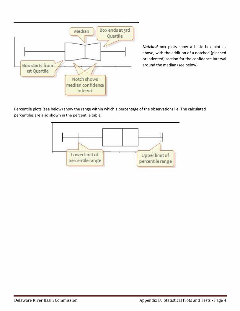
Basic box plots show a simple rectangular

box-plot, from the first to the third quartile,

with the median marked in the center (see

below).

Delaware River Basin Commission Appendix B: Statistical Plots and Tests - Page 4

Notched box plots show a basic box plot as

above, with the addition of a notched (pinched

or indented) section for the confidence interval

around the median (see below).

Percentile plots (see below) show the range within which a percentage of the observations lie. The calculated

percentiles are also shown in the percentile table.

Delaware River Basin Commission Appendix B: Statistical Plots and Tests - Page 5

Mean and Standard Deviation plots

Mean and SD plots show the parametric central tendency and dispersion.

The mean plot (left) shows the

mean as a vertical line, and

optionally, the confidence interval

for the mean as a diamond shape.

SD plots (left) are similar to non-parametric

percentile plots, but show the parametric

dispersion of the sample.

Delaware River Basin Commission Appendix B: Statistical Plots and Tests - Page 6

Assessing Normality

Normality can be visually assessed from the frequency histogram, or a Normal Quantile plot and a statistical hypothesis

test can be used.

The normality tests available are:

Shapiro-Wilk, recommended for sample sizes of up to 4000 observations.

METHOD The Shapiro Wilk test uses the modified Shapiro-Wilk method and so is suitable for moderate sample sizes (see

[4]).

Anderson-Darling, recommended for sample sizes larger than 4000 observations.

METHOD The Anderson-Darling goodness-of-fit test, modified for unknown population mean and variance, is used (see

[2]).

Kolmogorov-Smirnov, not recommend, mainly for historical interest.

METHOD The Kolmogorov-Smirnov goodness-of-fit test, modified for unknown population mean and variance, is used

(see [2]).

The normality test statistic and hypothesis test are shown. The p-value is the probability of rejecting the null hypothesis,

that the sample is from a normally distributed population, when it is in fact true. A significant p-value implies that the

sample is from a non-normally distributed population.

The Normal quantile plot shows the observations

of the sample against the expected normal

quantile. The expected quantile is the number of

SDs from the mean where such an observation

would be expected to lie in normal distribution

with the sample mean and standard deviation.

When the sample is normally distributed the

points will form a straight-line. Deviation from the

line indicates non-normality.

Delaware River Basin Commission Appendix B: Statistical Plots and Tests - Page 7

Correlation and association

Correlation explores the association between two or more variables and makes inferences about the strength of the

relationship.

For example, a teacher may want to examine the correlation between the number of hours sleeping and studying for a

group of students. A sociologist may want to examine the association between height and self-esteem. Similarly, a

medical researcher may want to examine the relationship between hemoglobin and packed cell volume in two groups of

women.

Note: The terms correlation and association are often used interchangeably. Technically, association refers to any

relationship between two variables, whereas correlation is often used to refer only to a linear relationship between two

variables. The terms are used interchangeably in this guide, as is common in most statistics texts.

Correlation coefficient

A correlation coefficient measures the association between two variables.

Scatter plot

A scatter plot shows the association between variables.

Inferences about association

A bivariate random sample of data drawn from a population can be used to make inferences about the

association between the variables in the population.

Scatter Plots (Annual Plots)

A scatter plot shows the association between variables.

You can use the plot to determine the type of association between variables. If the variables tend to increase and

decrease together, the association is positive. If one variable tends to increase as the other decreases, the association is

negative. When a straight line describes the relationship between the variables, the association is linear. When a

constantly increasing or decreasing nonlinear function describes the relationship, the association is monotonic. Other

relationships may be nonlinear or non-monotonic.

The type of relationship determines the statistical measures and tests of association that are appropriate. A bivariate

normal density ellipse summarizes the correlation between variables when the relationship is linear. The narrower the

ellipse, the greater the correlation between the variables. The wider and more round it is, the more the variables are

uncorrelated.

If the association is nonlinear, it is worth trying to transform the data to make the relationship linear as there are more

statistics for analysing linear relationships and their interpretation is generally easier.

You can also use a scatter plot to spot outliers. An individual observation on each of the variables may be perfectly

reasonable on its own, but appear as an outlier when plotted on a scatter plot. Avoid outliers as they badly affect the

Pearson product-moment correlation coefficient. Other correlation coefficients are more robust to outliers.

Delaware River Basin Commission Appendix B: Statistical Plots and Tests - Page 8

Fit model

Fit model describes the relationship between a response variable and one or more predictor variables.

Fits many models including simple linear regression, multiple linear regression, analysis of variance (ANOVA), analysis of

covariance (ANCOVA), and binary logistic regression.

For example, an engineer may want to determine the relationship between fuel consumption and various vehicle

factors. An economist may be interested in examining the link between employee salary and years in education using a

linear regression with an exponential fit. Or a scientist may study the effect of the dose of a drug for different age groups

using a logistic regression.

You can fit different types of model to the data:

Simple regression models

Advanced models

The tasks available depend on the type of analysis.

Linear fit

A linear model describes the relationship between a response variable and the explanatory variables using a

linear function.

Logistic fit

A logistic model describes the relationship between a categorical response variable and the explanatory

variables using a logistic function. The model is formulated in terms of the log odds ratio (the logit) of the

probability of the outcome of interest as a function of the explanatory variables.

Simple regression models

Simple regression models describe the relationship between a single predictor variable and a response variable.

Line Fit the model Y = b0 + b1 x. Fit a straight line.

Polynomial Fit the model Y = b0 + b1 x + b1 x2.... Polynomials are useful when the function is smooth but not straight. Any smooth function can be estimated by a polynomial of a high-enough degree. Polynomials are generally used as approximations and rarely represent a physical model.

Logarithmic Fit the model Y = b0 + b1 Log(x). Fit a logarithmic function curve.

Exponential Fit the model Y = a * b1x Fit an exponential function curve.

Power Fit the model Y = a * x b1. Fit a power function curve.

Logistic Fit the model Y = b0 + b1 x where x is the logit.

Delaware River Basin Commission Appendix B: Statistical Plots and Tests - Page 9

Linear fit

A linear model describes the relationship between a response variable and the explanatory variables using a linear

function.

Scatter plot

A scatter plot shows the relationship between variables.

Parameter estimates

Parameter estimates (also called coefficients, or beta coefficients) are the change in the response associated

with a one-unit change of the predictor, all other predictors being held constant.

Summary of fit

R² and similar statistics examine how well the model fits the data.

Lack of Fit

An F-test or X2-test formally tests whether the model fits the data.

Effect of model hypothesis test

An F-test formally tests the hypothesis of whether the model fits the data better than no model.

Predicted against actual Y plot

An effect of model plot shows the observed response against the response predicted by the model.

Effect of terms hypothesis test

An F-test formally tests whether a term contributes to the model.

Effect leverage plot

An effect leverage plot, also known as added variable plot or partial regression leverage plot, shows the unique

effect of a term in the model.

Residual plot

A residual plot shows the residuals (the difference between the observed response and the fitted response

values) against the predictor variable. Normality, sequence and lag plots of the residuals show additional

information about their behaviour.

Outlier and influence plot

An influence plot shows the outlyingness, leverage, and influence of each case.

Prediction

Predict the value of an individual future observation or to predict the population mean at specific values of the

predictors.

Delaware River Basin Commission Appendix B: Statistical Plots and Tests - Page 10

Summary of fit

R² and similar statistics examine how well the model fits the data.

R² is the proportion of variability in the response explained by the model. It is 1 when the model fits the data perfectly, though it can only attain this value when all observations for the predictors are different. Zero indicates the model fits no better than the null model. R² should not be used when the model does not include a constant term, as the interpretation is undefined.

For models with more than a single term, R² can be deceptive as it increases as more parameters are added to the model, eventually reaching saturation at 1 when the number of parameters equals the number of observations. Adjusted R² is a modification of R² that adjusts for the number of parameters in the model. It only increases when the terms added to the model improve the fit more than would be expected by chance. It is preferred when building and comparing models with a different number of parameters.

For example, if we fit a straight-line model, and then add an additional term to produce a quadratic polynomial model, the value of R² will increase. If we continued to increase the polynomial order to the same as the number of observations, then the R² value would be 1. The adjusted R² statistic is designed to take into account the number of parameters in the model and ensures that adding the new term has some useful purpose rather than simply due to the number of parameters approaching saturation.

In cases where there is more than a single set of predictors with the same value it may be impossible for the R² statistic to reach 1. A statistic called the maximum attainable R² indicates the maximum value that R² can achieve even if the model fitted perfectly. It is related to the pure error discussed in the lack of fit test

The standard error (SE) of the fit, also known as root mean square error (RMSE), is an estimate of the standard deviation of the true unknown random error. If the model fitted is not the correct model, the standard error will be larger than the true random error, as it includes the error due to lack of fit of the model as well as the random errors.

Delaware River Basin Commission Appendix B: Statistical Plots and Tests - Page 11

Frequency distribution

A frequency distribution reduces a large amount of data into a more easily understandable form.

A simple table of the frequencies may be all that is needed. Alternatively, there are a number of plots that highlight

different aspects of the distribution.

Cumulative distribution function plot

A cumulative distribution function (CDF) plot shows the empirical cumulative distribution function of the data.

Histogram

A histogram shows the distribution of the data.

Cumulative Distribution Functions

A cumulative distribution function (CDF) plot shows the empirical cumulative distribution function of the data.

The empirical CDF is defined as the proportion of values less than or equal to X. It is an increasing step function that has

a vertical jump of 1/N at each value of X equal to an observed value. You can use the plot to see the shape of the

distribution of the data, or to compare the shape of the distributions for different sets of data.

Delaware River Basin Commission Appendix B: Statistical Plots and Tests - Page 12

Equality of means / medians hypothesis test

A hypothesis test for equality of means/medians formally tests if the populations the samples represent have different

central location parameters.

The hypotheses to test depend on the number of groups to be tested.

For 2 groups, the null hypothesis states that the difference between the mean/medians of the groups is equal to

a hypothesized value (0 indicating no difference), against the alternative hypothesis that it is not equal to (or

less-than / greater-than) the hypothesized value.

For more than 2 groups, the null hypothesis states that the means/medians of the groups are equal, against the

alternative hypothesis that at least one group is different.

When the test p-value is small, you can reject the null hypothesis and conclude that the groups differ in central location.

It is important to remember that a statistically significant test tells you nothing about the practical importance of what

was observed. For a large sample, the difference detected by a statistically significant hypothesis test may be so small as

to be practically useless. Conversely, although there may be some evidence of a difference, the sample size may be too

small to reach statistical significance, and you may miss an opportunity to discover a true, meaningful difference. For

these reasons, it is essential that the p-value is always interpreted together with an estimate of the effect size, so both

statistical significance and practical importance can be evaluated.

Kruskal-Wallis Test if the medians of 2 or more groups are equal.

Assumes the population distributions are identically shaped, except for a possible shift in central

locations.

Wilcoxon-Mann-

Whitney

Test if the shift in location between 2 groups is equal to a hypothesized value.

When the population distributions are identically shaped, except for a possible shift in central

location, the hypothesis can be stated as testing for a difference in medians.

When the population distributions are not identically shaped the hypothesis can be stated as a test

whether the samples come from populations such that the probability is 0.5 that a random

observation from one group is greater than a random observation from another group.

Student t

(commonly used in

the past)

Test if the difference in mean between 2 groups is equal to a hypothesized value.

Assumes the populations are normally distributed. Due to the central limit theorem the test may

still be useful when the assumption is violated if the sample sizes are equal, moderate size, and the

distributions have similar shape. However, in this situation the Wilcoxon-Mann-Whitney test may

be more powerful.

Assumes the population variances are equal. The assumption can be tested using the Levene test.

The test may still be useful when the assumption is violated if the sample sizes are equal. However,

in this situation the Welch t-test may be preferred.

Delaware River Basin Commission Appendix B: Statistical Plots and Tests - Page 13

References to further reading

1. Handbook of Parametric and Nonparametric Statistical Procedures (3rd edition)

David J. Sheskin, ISBN 1-58488-440-1 2003.

2. Goodness of Fit Techniques

Ralph D'Agostino, Michael Stephens, ISBN 0-8247-7487-6 1986.

3. Approximating the Shapiro-Wilk W-test for non-normality

Royston P, Journal Statistics and Computing, Vol 2 No. 3 1992; 117-119.

4. Some Implementations of the Boxplot

Michael Frigge, David C. Hoaglin, Boris Iglewicz, The American Statistician Vol 41, No. 1 1989; 50-55.

5. Sample Quantiles in Statistical Packages

Rob J. Hyndman, Yanan Fan. The American Statistician, Vol. 50, No. 4 1996, 361-365.