appendix b review of public transport models f appendix b.pdf · review of public transport models...

DISTILLATE

PROJECT F

Appendix B

REVIEW OF PUBLIC TRANSPORT MODELS

April 2006

Author: J.D. Shires

1

Contents Page No. Introduction 4 Section 1 Simple Elasticity Models 6 1.1 Passenger Demand Forecasting Handbook (PDFH) 6 1.2 Area Review Model 7 1.3 Demand for Public Transport 8 Section 2 DfTGuidance on Public Transport Modelling 10 Section 3 Rail Models 12 3.1 The Framework Model (RIFF) 12 3.2 The Lythgoe Model 13 3.3 PRAISE (Privatised Rail Services) Model 14 3.4 National Rail Model (NRM) 15 3.5 Planet Suite 16 3.6 West Yorkshire METRO Model 17 Section 4 Bus Models 20 4.1 Economic Modelling Approach 20 4.2 Quality Bus Model 20 4.3 NERA & LEK Models for CfIT 21 Section 5 Multi-modal and Network Based Models 24 5.1 Road Traffic & Public Transport Assignment Models 24 - Principles 24

- Models 25 • PT-SATURN 25 • EMME/2 26 • TRIPS 27 • VIPS 27 • VISUM 27

5.2 Micro-Simulation Models 27 - Principles 27 - Models 28

• STEER 28 • DRACULA 28

5.3 Multi-modal Demand Models 28 - Principles 28 - Models 29

• METS 29 • MUPPIT 30

5.4 Land Use/Transport Intercation (LUTI) & Strategic Demand Models 31 - Principles 31 - Models 32

• MEPLAN 32 • TRANUS 32 • TPM 33 • MARS 33 • START/DELTA 34 • STM 34

Section 6 Comparison of the Models & Research Gaps 35 6.1 Rail Models 40 6.2 Bus Models 40 6.3 Simple Elasticity Recommendations 40 6.4 Multi-modal Modals 41

6.4.1 Road Traffic & Public Assignment Models 41

2

6.4.2 Micro-Simulation Models 41 6.4.3 Demand Models 41 6.4.4 Land-Use/Transport Interaction (LUTI) Models 41

6.5 Gaps in Research 47 6.5.1 General Gaps 47

(a) Lifestyle Impacts 47 (b) Soft Variables 47

6.5.2 Rail Models 47 6.5.3 Bus Models 48 6.5.4 Multi-modal Models 48 6.5.4.1 Road Traffic & Public Transport Assignment Models 48

6.5.4.2 Micro-simulation Models 48 6.5.4.3 Demand Models 48 6.5.4.4 LUTI Models 48

7 The Way Forward in Distillate 50 7.1 PT-Saturn & Quality Bus Case Studies 50 7.2 MARS Case Studies 50 7.3 METRO Heavy Rail Model Case Studies 51 7.4 Dracula Case Studies 51 7.5 STEER Case Studies 51 7.6 STM Case Studies 51 References 52

3

Introduction: This report reviews a wide range of public transport models covering a number of modes and purposes. In order to facilitate comparison the models are split into the following categories:

1) Simple Elasticity Models 2) Rail Models 3) Bus Models 4) Multi-modal & Network Based Models 5) General Guidance

Within each category there are a wide range of demand based models ranging from simple static elasticity models to more complex dynamic, network based models which consider both supply and demand. The list of models reviewed is outlined in the Table below. Table A Outline of Models Reviewed Model Simple Elasticity Models 1.1 Passenger Demand Forecasting Handbook (PDFH) 1.2 Area Review Model Handbook (PDFH) 1.3 The Demand for Public Transport: A Practical Guide Rail Models 2.1 The Framework Model (RIFF) 2.2 The Lythgoe Model 2.3 PRAISE 2.4 National Rail Model 2.5 PLANET Suite 2.6 METRO Model Bus Models 3.1 EMA 3.2 Quality Bus Model 3.3 NERA & LEK Models for CfIT 3.4 The London Bus Model Multi-Modal & Network Based Models 4.1 Road Traffic & Public Transport Assignment Models (a) PT-SATURN (b) EMME/2 (c) TRIPS (d) VIPS (e) VISUM 4.2 Micro-Simulation Models (a) STEER (b) DRACULA 4.3 Demand Models (a) METS (b) MUPPIT 4.4 Land Use/Transport Interaction (LUTI) & Strategic Demand Models

4

(a) MEPLAN (b) TRANUS (c) TPM (d) MARS (e) START/DELTA (f) STM

5

Section 1 Simple Elasticity Models In this section we review simple elasticity models which tend to be based around static frameworks around which constant elasticities are applied. The three examples outlined below are prescriptive in nature and provide general recommendations for a range of public transport modelling assignments. 1.1 Passenger Demand Forecasting Handbook (PDFH) The PDFH dates back to the early 1980s and is currently formulated and produced by the Passenger Demand Forecasting council (PDFHC, 2002), who bring together representatives from the Train Operating Companies (TOCs), Network Rail, the Strategic Rail Authority, Transport for London and the Office for the Rail Regulator. The handbook summarises best practise demand forecasting for rail when considering the effects of service, quality, fares and external factors (such as GDP). It is industry standard and often used assisting with decisions on investment, marketing, fare setting etc….and assessing customer responses to timetabling and operating decisions. The PDFH recommends a static framework for the application of elasticities of demand and rail attribute valuation to facilitate forecasts of aggregate demand changes, usually based on annual data (although the user can compound annual changes to yield forecasts for any desired time horizon). The handbook provides specific parameters for a range of factors including:

• The external environment • Fares elasticities • Journey time/frequency/interchange • Reliability • Non-timetable related service quality • New services/access • Competition between operators

For each of these factors, the PDFH provides a theoretical background, a mathematical framework, a set of recommended parameters, simple and more complex forecasting and applications. Recommended parameter values vary in many dimensions, such as journey purpose, ticket type, distance, GDP, income and competition and flow type. The recommended parameters are disaggregated by regions to reflect differences in the make up of those services. These regions are outlined below:

• London Travel card area • South East • Rest of the country to London flows (by distance bands) • Non-London Inter-Urban flows with/without full set of tickets (by distance

band) • Airports • Rest of the country

6

When producing forecasts the user must provide values of variables such as generalised time components, fares, service quality and macro economic factors such as car ownership, GDP, costs and journey times of competing modes. A simple example is outlined below: Example 1: GJT has increased from 183 minutes to 225 minutes. Using a GJT elasticity of -0.9, the forecast change in demand is:

74.0183255 9.09.0

=⎟⎠⎞

⎜⎝⎛=⎟

⎠⎞

⎜⎝⎛=

−−

base

newj

GJTGJTI

PDFH, 2002 The PDFH is a unique collection of models brought together under a single umbrella to provide general advice to rail practitioners. Whilst the static nature of the models and their focus only upon the demand side maybe viewed as limiting by some transport professionals they provide very good estimates of demand over the short term and are constantly updated via a thorough research agenda which commissions research on a rolling out basis. They are also simple to apply and do not needs any software (although a piece has been developed for those wishing to use it, called PDFHAT). 1.2 The Area Review Model Handbook (ITS, 2003) This was commissioned by First and has two major components. Firstly a handbook based along similar lines to the Rail PDFH which explains in depth to the transport practitioner six sets of factors which effect bus demand and provides elasticities and methodologies which can be used to estimate such effects. The effects are outlined below, • Fare changes. • Timetable changes • Quality changes. • Cross modal competition. • Competition from other bus users • External Influences. The second component is the Area Review Model which takes the form of an excel based spreadsheet model. The model is capable of estimating the demand changes that result from changes in the six categories of factors outlined in Section B. The model can handle multiple changes in demand factors, ticket types and time periods (see Table 1.1).

7

Table 1.1 Ticket Types & Time Period Examined by the ARM Ticket Type Time Period Adult (full fare) Child Day ticket Adult (concession) Adult (multi-trip including seasons)

AM peak Interpeak PM peak Evening Night

The model inputs consist of bus operating data for the route or service being examined plus the behavioural parameters (elasticities, value of time) outlined by the handbook. The bus operating data requirements for the base period are outlined below and apply to each market segment on that route/service.

• Demand (number of trips). • Revenue per passenger (i.e. average fare). • Bus miles. • Bus hours. • Average trip length. • Interworking factors (i.e. the degree of overlap with other routes).

The main outputs of the model include measures of changes in:

• Demand (disaggregated by ticket type and time period). • Revenue (disaggregated by ticket type and time period). • Consumer Surplus (user benefit). • Externalities (accidents and pollution).

Demand and revenue are forecast for each month up to six months following the specified changes, then one year on. 1.3 The Demand for Public Transport: A Practical Guide (TRL, 2004) This guide was commissioned as a follow up to a TRL report, The Demand for Public Transport (the Black Book) which was published in 1980. That particular report was widely recognised as a seminal piece of work covering demand evaluation, but with changes to many of the parameter values and methodologies it contained it was recognised that an update was due. The overall objectives of the new study were to: “

• Undertake analysis and research by using primary and secondary data sources on the factors influencing the demand for public transport.

• Produce quantitative indications of how these factors influence the demand for public transport.

• Provide accessible information on such factors for key stakeholders such as public transport operators and central and local government.

• Produce a document that assists in identifying cost-effective schemes for improving services”

TRL, 2004

8

The review presents its findings as a series of chapters which tend to present evidence and recommend values of particular types of elasticities or parameter values (i.e. quality values); before recommending how to implement these in determining public transport demand. The key areas covered by the chapters include:

• Effect of Fares on PT Demand; • Effects of Quality of Service: Time Factors on PT Demand; • Effects of Quality of Service: Other Factors on PT Demand; • Effects of Demand Interactions on PT Demand; • Effects of Income and Car Ownership on PT Demand; • Relationship Between Land-Use and Public Transport; • New Public Transport Modes; and, • Effects of Other Transport Policies.

9

Section 2 DfT Guidance on Public Transport Modelling The Department for Transport (DfT) issues guidance on both demand modelling (VADMA) and on public transport modelling (WebTag). The former is covered by appendix A of DISTILLATE Deliverable F2 (Shepherd et al, 2006), whilst the latter is briefly outlined here. WebTag is the Department for Transport’s website for guidance on the conduct of transport studies, specifically for the appraisal of transport projects and more generally for the scoping and carrying out of general transport studies. According to the site (www.webtag.org.uk) the guidance should be seen as a best practise guide and supersedes a number of existing documents including:

• The Guidance on the Methodology for Multi-Modal Studies (GOMMMS). • Applying the Multi-Modal Approach to Appraisal to Highway Schemes. • Major Scheme Appraisal in Local Transport Plans.

It provides advice on how to: “

1. Develop potential solutions. 2. Create a transport model for the appraisal of the alternative solutions. 3. How to conduct an appraisal which meets the Department’s requirements.”

www.webtag,org.uk (DfT, 2005) In terms of public transport modelling there are a number of documents that provide guidance on best practise these are outlined below: (a) TAG Unit 1.1 Introduction to Transport Analysis (DfT, 2005) This provides an introduction to the principals of transport analysis and can be found at : www.webtag.org.uk/webdocuments/1_Overview/1_Introduction_to_Transport_analysis/index.htm (b) TAG Unit 2.1 The Overall Approach: Steps in the Process (DfT, 2005) This presents a flow diagram outlining the appraisal process and where public transport modelling fits in. www.webtag.org.uk/webdocuments/2_Project_Manager/1_Overall_Approach_Steps/index.htm

(c) TAG Unit 2.4 Summary Advice on Modelling (DfT, 2005)

10

http://www.webtag.org.uk/

http://www.webtag,org.uk/

http://www.webtag.org.uk/webdocuments/1_Overview/1_Introduction_to_Transport_analysis/index.htm


http://www.webtag.org.uk/webdocuments/2_Project_Manager/1_Overall_Approach_Steps/index.htm


This introduces the models to be used in the appraisal process and includes a discussion on, “…the general principles of transport modelling, the general principles of land-use modelling, and the choice of modelling approach”.

www.webtag.org.uk/webdocuments/2_Project_Manager/4_Summary_Advice_on_Modelling/index.htm

(d) TAG Unit 3.1.2 Transport Models (DfT, 2005)

This outlines the general principles of transport modelling and then goes on to focus on spatially detailed models and spatially aggregate models, before providing advice on forecasting.

www.webtag.org.uk/webdocuments/3_Expert/1_Modelling/3.1.2.htm

(e) TAG Unit 3.1.3 Land Use/Transport Interaction Models (DfT, 2005)

This outlines the general principles of land-use models and also the different forms of land use/transport (LUTI) models.

www.webtag.org.uk/webdocuments/3_Expert/1_Modelling/3.1.3.htm

Taken together the documents represent a comprehensive mass of state of the art guidance material and are very useful tools.

11

http://www.webtag.org.uk/webdocuments/2_Project_Manager/4_Summary_Advice_on_Modelling/index.htm


http://www.webtag.org.uk/webdocuments/3_Expert/1_Modelling/3.1.2.htm


Section 3 Rail Models There are a wide range of rail models, many of which have been developed over time, building up a wide experience of knowledge in all areas (PRAISE) and many which are context specific (Lythgoe’s Parkway model) to certain types of traffic or route. 3.1 The Framework Model (SDG, 1999) This model was developed in 1999 by transport consultants Steer Davis Gleave and is based on changes to fares and service levels using bespoke software based upon an Access Database with an Excel/Visual Basic front end. The results of the research into elasticise for the model have since been incorporated into the PDFH. The model itself is an aggregate demand model, based around O-D zones and the passenger flows and track and service network links between them. In addition service and demand elasticities are overlaid onto the O-D zones. Whilst the model is uni-modal, it is able to incorporate the effect of competition from other modes via cross-elasticities. Demand for year I is estimated based on a set of demand drivers, for which elasticities are required. Also included is the proportional change in demand due to timetable changes, the growth in year (due to population changes) and the residual growth in year I to i+1. A set of appropriate elasticities are required for each demand driver, differentiated by flow category and trip purpose. Cross mode effects can also be captured using this formulation. If demand drivers are defined describing conditions on competing modes, and cross-mode elasticities are available. The modelling encompasses the whole of the GB rail network by the zoning and degree of aggregation is entirely up to the user and will typically vary by the scope of the case study and the data availability. The model can forecast for whatever time frame the user specifies, but will require estimates of future variables such as population, employment, car ownership and car running cost. The model uses information from existing data sources, including: • CAPRI – which provides information on base year flows of passengers and

revenues by operator and ticket type, with tickets broken up into full, seasons, standard class, standard class advanced purchase/promotional and miscellaneous.

• SCORES – which provides information about changes in components of travel time as future time-tables are introduced.

• MOIRA – as an alternative source of information on the effects of future service levels.

In addition econometric analysis carried out by the Centre for Economics and Business Research (CEBR, 1998) as part of the RIFF (Rail Industry Forecasting Framework) project provided some new evidence on fares elasticities, GDP & population elasticities linked with journey purpose, and car ownership and congestion elasticities which were previously subsumed in a generic time trend. The model also incorporates some proposed cross-elasticities to the costs and service characteristics

12

of other modes. These have been estimated using the diversion factors approach. Other values were taken from the PDFH. When run, the model delivers a database of flows between the zones which are differentiated by origin and destination zones; ticket category; trip purpose; route number; year, trips and revenue, allowing the user to estimate the impacts on demand from changes to fares and service levels. The RIFF model is useful for examining the impact of changes to fare and service levels on the national rail network as a whole. It is very data intensive which reduces it’s suitability to be run and also dictates the level of disaggregation. 3.2 The Lythgoe Model The Lythgoe model was developed at the Institute for Transport Studies, University of Leeds, with the specific aim of estimating rail demand from new parkway rail stations (Lythgoe & Wardman, 2004). As such it forms the basis of the Parkway Stations section in the PDFH. Since then a version of the model has also been used to assess the impact of regular interval timetables on the East Coast Mainline. The model was developed using FORTRAN and whilst the source code is available there is no user-friendly front end. The model is an aggregate origin choice demand model estimated on data based on polygonal population zones around the origin station but with destination station dummies. The model is capable of forecasting rail passenger demand for new and adjusted rail services including those involving a new origin or destination stations. The model has a cross-nested logit structure which allocated the share of total rail demand between competing origin stations and allows the overall size of the rail market to expand or contract as rail fares and quality of service change. The cross-nested specification is developed to model differing degrees of dissimilarity between station choice pairs. This more generalised model form allows for differing degrees of competition between different origin stations. The logit specification also allows the application of population elasticities. The model itself is uni-modal and whilst it takes into account the impact of the car, the outputs are constrained to rail demand. The model explains the trips between two stations in terms of some or all of the following:

• Fare and timetable related service quality and competing origin stations to the destination station. This includes measures of service regularity, clockfaceness and memorability, using values from stated preference research.

• Population in zones around origin and destination stations. • Access times and distances from origin population zones to origin and

competitor origin stations. • Egress times and distances from destination and competitor destination

stations to destination population zones. • Alternative car journeys.

Since the model is O-D based, it can estimate the demand between any pair of stations, subject to availability of data. The model covers the whole of the GB rail

13

network and has a zoning system of 16 zones around each station. The model estimates annual changes to the demand forecasts but requires data on population for the station catchment area, fares, generalised journey time and car costs. The Lythgoe model was developed for a specific purpose and has been very successful in developing new forecasts for Parkway rail stations. In addition the same principals have been used to develop its capabilities in other areas such as interval timetabling. This adaptability has made it very useful to the transport practitioner. It is however quite specific in its output – absolute demand – which can sometimes be too aggregate a measure. It is also not user friendly and requires some understanding of FORTRAN and its underlying modelling principles. 3.3 PRAISE (Privatised Rail Services) Model The PRAISE model was developed at the Institute for Transport Studies, University of Leeds and is driven by a Windows based user interface and requires the prior installation of ACCESS and permission from the SRA in order to access the supplied stopping pattern, fares, elasticities and demand databases which it uses. The model was initially developed to examine the potential for ‘open access’ competition on the railways following the privatisation of rail services (Whelan et al. 1998), in particular the Leeds to London corridor. It has since been applied to other routes in the UK (Gatwick Express) and overseas (Stockholm to Gothenburg) and to other areas such as valuing scarcity on the East Coast Main Line (Johnson & Nash, 2005); the effect of ticketing policies on overcrowding (Whelan and Johnson, 2004). PRAISE is in fact a suite of models that combine together to produce estimated outputs. It comprises of a disaggregate demand model, a cost model and an evaluation model. The demand model has a hierarchical structure and works at the level of the individual traveller. Using information on passenger’s valuation of journey attributes, together with elasticities, the lower level of the model assigns a probability that a traveller will choose a particular ticket and outward and return service combination. By aggregating these probabilities over a representative set of simulated passengers, the model forecasts market shares for each service and ticket combinations. The upper level of the model allows the rail market to expand or contract according to the overall level of service. By assessing the outward and return portions of the journey, together with information on ticketing restrictions (departure time, advanced purchase, transferability between operators), the model is able to forecast ticket revenue by operator. The demand model is calibrated to existing data on market shares and elasticities. The cost model employs a cost accounting approach incorporating, costs that are related to operating hours, train kilometres and fixed costs. Costs can be varied by operator and rolling stock type. The model generates output that can be used in a formal appraisal system, including user benefits, operating profits but not external costs. The user of the model builds up the networks by introducing OD pairs into the analysis as opposed to networks. As such the focus of the model will tend towards the route level or simplifications of networks. The run times for any substantial network

14

become too large and are unworkable. The forecasts produced by the model are based upon daily changes and are seen very much as short run in nature. The major inputs into the model require data from the railway industry, specifically current demand data for different OD pairs (provided by CAPRI); operator costs expressed in terms of average cost per train km or per hour (sourced from the Rail Industry Monitor); market shares for each operator (sourced from CAPRI); current fares (sourced from CAPRI); and journey opportunities for each OD pair (sourced from the SRA). Other parameters and elasticities were taken from the PDFH. The outputs of the model are quite detailed and allow a social cost benefit analysis to be undertaken. They include changes:

• To passenger demand (at OD level). • To passenger kms (at OD level). • To operator revenue (at OD level). • To operator costs (at OD level). • To operator profitability (at OD level). • In rail user benefits (consumer surplus). • In over crowding (at OD level); and • Modal transfers.

The characteristics of the PRAISE model mean it is much more suited to modelling routes or small networks than models such as the Framework model which tend to focus upon the network as a whole. The wide range of outputs mean it is very useful for carrying out appraisals, whilst the ability to model a range of policy variables make it extremely versatile for the transport practitioner. It does however require substantial data from the railway industry and its run times are extensive which limits its capacity to model more complex networks 3.4 National Rail Model (NRM) The NRM (DfT, 2005g) was developed by Faber Maunsell on behalf of the Department for Transport as part of the Department’s multi-modal modelling capability and is viewed very much as a strategic model. The model is owned by the Department and is now part of the National Transport Model (DfT, 2005h and EMME/2 (INRO, 2005). To date the NRM has been developed as part of the Department’s multi-modal modelling package to test the Government’s TEN Year Plan strategies. The NRM is part of the Government’s National Transport model which represents a series of options faced by travellers in different circumstances including how far to travel, what area type to travel to and which mode of travel to use to get there (car driver, car passenger, rail, bus, cycle, walk). The model is in fact a series of models the most important being the mode choice and trip assignment models. The former generates a multi-modal trip matrix based on modal costs and then passes this to the EMME/2 assignment package that loads passengers onto the network of services. The assignment is based upon the concept of ‘optimal strategies’ whereby passengers choose a set of paths through the network and board the first train to arrive at their destination. The algorithm identifies a set of attractive alternative and then distributes

15

the demand amongst the attractive routes. The process is iterative so when policy variables are tested that change generalised costs these are then passed back to the multi-modal choice model where the modal shares are re-estimated. The NRM covers all national rail and London Underground stations and is based upon 1998 trip data. There are 1,318 zones within the model, with very detailed disaggregation around Greater London and other large cities. The data outputs are compatible with the TUBA cost-benefit program and largely take the form of changes in the number of trips by distance and purpose. 3.5 Planet Suite (SRA, 2002) This model was originally commissioned by the British Rail and was based around the 1991 National Rail Timetable. It has subsequently been developed by transport consultancies Jacobs and Atkins on behalf of the Strategic Rail Authority (SRA). The model requires the PLANET software package and the EMME/2 software environment. It has been used by the SRA to evaluate many projects including:

• Thameslink 2000. • CrossRail Business Case. • Strategic Plan 2003. • European Rail Traffic Management System (ERTMS). • Great Western Route Modernisation. • East-West Midlands Multi-modal study.

The Planet Suite is a set of network assignment models consisting of morning and inter-peak South and North models used for the forecasting and appraisal of rail schemes in the UK. It has a current forecasting mode for base demand and a forecast mode for estimating changes in travel demand arising through the switching between rail services, changes in mode split and trip distribution. Outputs are then used to populate an appraisal template. Planet Strategic also contains an incremental mode choice modal. The model is used to test policy variables such as changes to fares, service frequency, new services and new infrastructure. A typical full model run would see the model assigning a base demand matrix to the rail network (Planet covers the total GB rail network). The EMME/2 network assignment package loads a passenger demand matrix to a network of rail services in an iterative manner, taking account of capacity and crowding constraints. The assignment procedure in EMME/2 is based on the concept of a ‘strategy’: for any particular journey a set of ‘attractive lines’ is calculated, and a passenger then boards the first vehicle to arrive from any of these lines. Base generalised journey time matrices are then estimated which are passed to an elasticity model to estimate the demand impact of changes to the network. The revised demand matrix is then passed back to the assignment model to be loaded onto the network to generate passenger and train based outputs. These are presented by operator and rail/underground service groupings. There are four demand matrices included in the assignment procedure, business, commuter, leisure and total demand. Each demand matrix is assigned separately to calculate journey specific crowding factors. These are combined and weighted to

16

calculate overall crowding factors in the scenario. Crowding takes account of the multiple journey purposes, so there are separate demand and supply profiles for each journey purpose and service categories, with separate profiles for Underground demand and supply. The zoning system used by the Planet suite is based on 1600 zones in Planet North and 1400 in Planet South and covers the morning peak (0700-0959) and inter-peak (1000-1559) separately. The Planet Strategic add-on has 250 zones and is an all day model. In terms of inputs Planet requires the train service database to create ‘transit lines’ containing information on TOC, CAPRI service group, key station and direction for each node passed through. It also requires Computer Analysis of Passenger Revenue Information (CAPRI) for station to station ticket sales; and Operational Research Computer Allocation of Tickets to Services (ORCATS) used to factor daily demand to AM/IP periods. It’s elasticity sub model also requires GDP and fare elasticities for each journey purpose, whilst the appraisal template requires values of time for different journey purposes which are based on the PDFH and the DfT’s Transport Economics Note (TEN). Outputs from the model include estimates of passenger kms, total passenger hours, un-crowded passenger hours, crowded passenger hours, passenger boardings and train kms, and generalised journey times by purpose. Zonal outputs from Planet are generated at three levels: local area, sub-region and region. In addition the path between any two individual nodes can be analysed using the disaggregate analysis of trips. In terms of appraisal the output and cost inputs from the model are converted into value for money measures which can be used in a full economic appraisal. The PLANET suite of models is highly regarded within the rail industry and is seen as the SRA’s main model for carrying out major policy appraisals that will have national implications. The model is very data intensive and requires specific software that means its use tends to be restricted to within the rail industry. 3.6 West Yorkshire METRO Model This was originally developed by transport consultant’s SDG with further developments added by transport consultant’s JMP and the Institute for Transport Studies, University of Leeds, as part of the ‘Rail in the City Regions’ report commission by the PTEs in 2004 (JMP, 2004). As part of this study several policies affecting the suburban rail network serving Leeds and its conurbations were evaluated. These included:

• Additional rail services. • Improvements in rail journey times. • New infrastructure. • Reduction in crowding levels on trains. • Replacement of trains by buses (bustitution). • Changes to external factors, i.e. GDP growth.

17

The model is a constant elasticity model, based around a sophisticated excel spreadsheet. The spreadsheet has numerous connected sheets that can be classified under two category headings. These are outlined below. 1) Base Input Date

• This includes CAPRI rail demand data for eight lines (Airedale & Wharfedale, Harrogate, York & Selby, Pontefract, Caldervale, Hallam, Wakefield & Doncaster and Huddersfield) under considerations split by peak and off-peak.

• Base demand data for car and bus, again split by peak and off-peak. • Current rail service frequencies. • Current generalised journey times for rail, car and bus. • Current operating costs data for rail. • Current infrastructure and rolling stock cost data for rail. • Current levels of population (taken from TEMPRO). • Current GDP & employment levels in Leeds. • Current highway congestion levels • Current levels of overcrowding on rail services.

2) Behavioural Values (mainly taken from the PDFH)

• GJT elasticities. • Cross modal demand elasticites • GDP demand elasticities • Values of time • Population demand elasticities

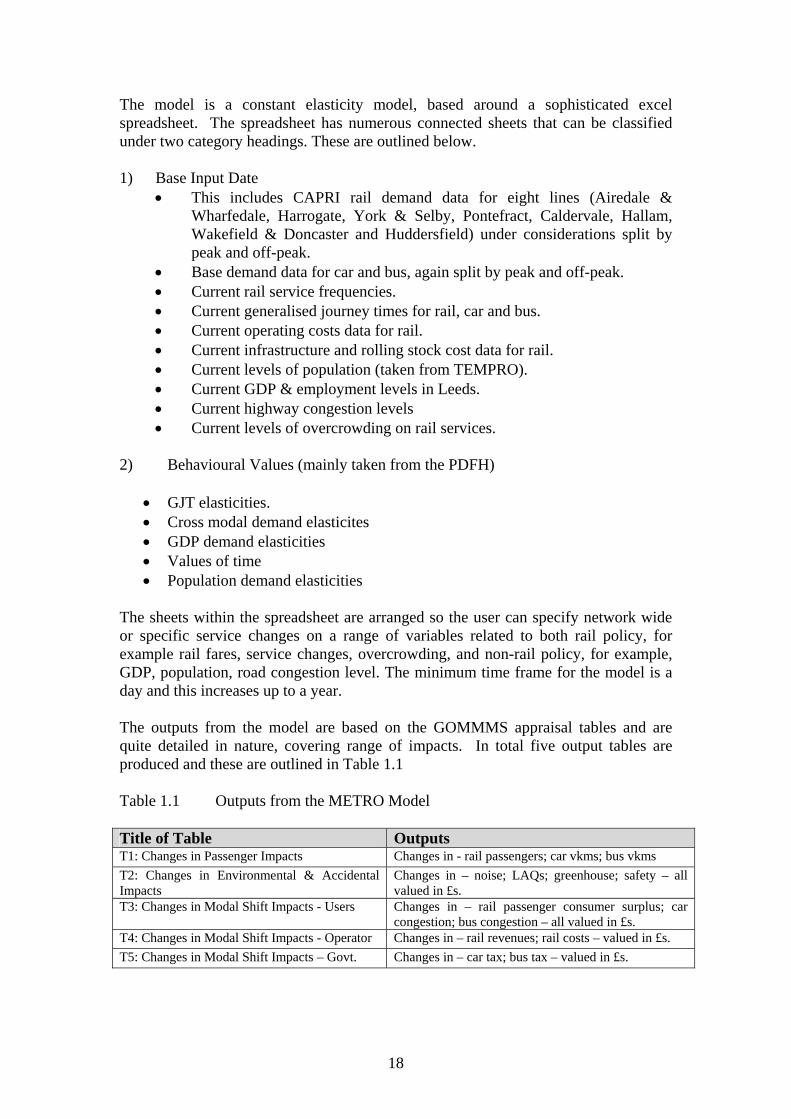
The sheets within the spreadsheet are arranged so the user can specify network wide or specific service changes on a range of variables related to both rail policy, for example rail fares, service changes, overcrowding, and non-rail policy, for example, GDP, population, road congestion level. The minimum time frame for the model is a day and this increases up to a year. The outputs from the model are based on the GOMMMS appraisal tables and are quite detailed in nature, covering range of impacts. In total five output tables are produced and these are outlined in Table 1.1 Table 1.1 Outputs from the METRO Model Title of Table Outputs T1: Changes in Passenger Impacts Changes in - rail passengers; car vkms; bus vkms T2: Changes in Environmental & Accidental Impacts

Changes in – noise; LAQs; greenhouse; safety – all valued in £s.

T3: Changes in Modal Shift Impacts - Users Changes in – rail passenger consumer surplus; car congestion; bus congestion – all valued in £s.

T4: Changes in Modal Shift Impacts - Operator Changes in – rail revenues; rail costs – valued in £s. T5: Changes in Modal Shift Impacts – Govt. Changes in – car tax; bus tax – valued in £s.

18

The METRO model was designed to provide short run, static analysis for the West Yorkshire PTE. In particular it was designed to enable users to run a variety of policy measures, and to provide a comprehensive appraisal of such measures that could fit into local transport plans. The downside of the model is that its analysis is not dynamic which means its forecasts may not be accurate in the medium to long term, and whilst the modelling framework it uses could be used for other PTEs, it would need populating with the correct base data, so it is essentially a location specific model. Any future development of the model should look at introducing a dynamic nature into the nature or a more sophisticated modal choice element which the current model lacks.

19

Section 4 Bus Models 4.1 Economic Modelling Approach (Dodgson, 1993)

The Economic Modelling Approach (EMA) was developed at Liverpool University by Dodgson, Katsoulacos and Newton (1993). The specific objective was to model and identify predatory behaviour in the bus industry. The model uses two alternative forms of operator-specific direct demand models with own and cross-price and service (bus-miles) elasticities for each of the two operators included. The EMA can demonstrate the situations in which either, both or neither of the incumbent and the entrant are able to make profits and hence check whether either (or both) are deliberately foregoing profits. The demand for each operator’s services is taken as a function of their own fare and level of service (bus miles) and the fares and level of service of the competing operator. By making assumptions about the functional form for the demand model (double log or negative exponential), together with assumptions regarding the own price elasticity, value of schedule adjustment time, value of in-vehicle time and value of wait time the cross elasticities between operators, for a given timetable and set of fares, are inferred using a Hotelling-type framework. The model was subsequently used to assist the OFT in some of its investigations into allegations of predatory behaviour in the bus industry. 4.2 Quality Bus Model (ITS, 2001)

The Quality Bus Model (Whelan et al, 2001) was initially developed by ITS Leeds for the Department for Transport to assess the potential impacts of quality bus partnerships. Subsequently the model has been applied in a study of subsidy allocation on behalf of the Commission for Integrated Transport. The software comprises a demand model, a cost model and an evaluation model. The demand model has a hierarchical logit structure and works at the level of the individual traveller. Using information on passengers’ valuation of journey attributes, such as journey time and schedule adjustment time, together with elasticity estimates, the lower level of the model assigns a probability that a given traveller (simulated with a given set of tastes and preferences and preferred departure time) will choose a particular service and ticket combination. By aggregating the ticket and service probabilities over a representative set of simulated passengers, the model is able to forecast market shares for each service and ticket combination. To allow for the fact that changing fares and services will change the overall demand for bus travel, the upper level of the model is structured to allow for the bus market to expand or contract according to the overall level of service. The cost model employs an accountancy cost approach (the CIPFA approach) incorporating costs that are related to operating hours, costs that are related to bus kilometres, and costs that are related to fixed costs (or costs that are related to peak vehicle requirement). Where load factors reach a threshold value (set by the user), the

20

cost of relief buses are provided. Costs can be varied by operator and are combined with estimates of revenue to generate forecasts of operator profitability. The model generates output that can be used in a formal appraisal system. This output includes, passenger demand, passenger distance, operator revenue, operator costs, profitability, user benefits (consumer surplus), overcrowding, and diversion to and from other modes in terms of passenger numbers and passenger distance. The model is written in Turbo C and can be applied to a wide range on bus networks across different operating periods. The user is free to define networks involving up to 50 stops and specify a set of behavioural and operational parameters to suit local circumstances. The behavioural parameters can be set for each simulated individual traveller or specified for key market segments (e.g. car available and non car available). The network timetable can include services from up to five different operators, each offering up to five different tickets with different availability by market segment (e.g. concession and non-concession) and time period (e.g. peak, off peak). In practice, the model has been applied to seven routes, including:

• A radial route in a large city (13 zones and 4 time periods)

• An orbital route in a large city (16 zones and 4 time periods)

• A radial route in a medium sized city (9 zones and 4 time periods)

• A radial route in a small city (18 zone and 4 time periods)

• A rural (13 zones and 3 time periods)

• An inter urban route (35 zones and 4 time periods)

• A park and ride service (4 zones and 2 time periods)

The model has usually been applied to key operating periods (Monday to Friday peak and off peak, Saturday and Sunday) but it has the capability to forecast demand and revenue by service and ticket type across a continuous 24hour period. The model can be run in batch mode where a number of operator strategies (fares, timetable related quality and vehicle related quality) need to be examined.

4.3 NERA & LEK Models for CfIT (ITS, 2002)

NERA’s & LEK’s models for CfIT were developed by ITS Leeds (Bristow, 2002). The model was developed with the specific aim of assessing the impact on bus operator profitability of a switch from Fuel Duty Rebate to a per passenger subsidy, and the consequent actions that the operator would take as a result of changed incentives. These actions are modelled using an optimisation procedure in which the

21

model manipulates input variables price, frequency and quality to maximise profit, subject to a number of possible constraints. There is no evaluation of bus user benefits nor of external benefits or costs. The model is route-based. Data on actual individual routes were obtained and used to model behaviour on those routes. The demand function used was of the negative exponential form. Given that the purpose of the study was to help understand bus operators’ reactions to the proposed change in terms of their fares, service and quality levels, the variables price, frequency and quality were used as explanatory variables in the demand (and cost) functions (rather than having these variables entering the demand function indirectly via the concept of generalised cost). The model used the same CIPFA-based cost allocation models with costs based on bus-kms, bus-hours and the peak vehicle requirement (PVR) as the Leeds Quality Bus Model. However, the number of vehicle hours in the model was made dependent on the number of passengers via an assumed boarding time per passenger (of three seconds). The purpose of this was to avoid a zero marginal cost per passenger, which could create problems when optimising. The cost model also took the costs of providing quality explicitly into account, and introduced a relief cost function that added the costs of relief buses to total costs once load factors exceeded a certain value. The purpose of the relief cost function was to avoid the model predicting profit-maximising combinations of price, frequency and quality that would involve unrealistically high load factors. Relief costs were a function of the ratio of modelled versus current load factor. The optimisation model uses the Solver routine in Microsoft Excel and is able to maximise profits by manipulating the price, buses per hour and quality variables, subject to a number of constraints. Certain constraints are imposed at every optimisation round. These are that the price charged and the quality level should be positive. Other constraints can be imposed at the discretion of the user. There are four possibilities: • Maximise profit. In this case, it is possible to impose the constraint that the

frequency should be an integer. This constraint can be imposed because in the vast majority of cases, the frequency per hour that operators run is indeed an integer. However, it is not necessary to impose this constraint, and allowing frequency to vary continuously allows the user to evaluate how the change in subsidy system will affect marginal incentives to increase or decrease frequency;

• Maximise profit subject to bus frequency equal to a certain value. With this option, the desired frequency can be entered and the model optimises by holding frequency constant and manipulating just the other two variables, e.g. one bus per two hours (in which case the value to be entered is 0.5);

• Maximise profit subject to price equal to a certain value. This option holds price constant and manipulates frequency and quality. This option is useful if

22

the operator chooses to set prices below profit-maximising levels, possibly to deter entry or for political reasons;

• Maximise profit subject to quality equal to a certain value. With this option, only fare and frequency are manipulated. This option can be used if there is no scope for changing the quality level offered, for example if new buses have just been introduced on the route which are not going to be modified in the short or medium term.

The model produces a route profitability sheet which shows passenger, revenue, costs, profits and returns on sales. It also shows the profit-maximising combination of fares, frequency and quality levels.

23

Section 5 Multi-modal Models There are a range of models which come under the heading of multi-modal, which by definition mean they examine more than one mode of transport. It is often the case that these models contain a number of distinct components for example,

1) A road traffic & public transport assignment model; 2) A traffic micro-simulation model; 3) A demand model; 4) A land use/transport interaction models.

There are further distinctions to be made within each individual component, for example, land use/transport interactions models maybe ‘activity based’ or ‘spatial economic based’ (David Simmonds & MEP, 1999). A number of modelling packages are based around the same distinct components outlined above and vary very little between each other. In order to prevent repetition this report now outlines the principles behind each modelling component before then briefly reviewing (and sometimes listing) the modelling packages themselves with respect to their public transport elements. 5.1 Road Traffic & Public Transport Assignment Models Principles: A number of assignment models exist and they can be used to model a range of networks from assessments of local junctions to large scale city networks. The basic theory behind assignment models is based upon the actual exchanges of goods and services (supply & demand) and obtaining an equilibrium point where the, ‘…marginal cost of producing and selling the goods equals the marginal revenue obtained from selling them’ (Ortuzar & Willumsen, 2001). Placing this into a transport context sees a supply side consisting of a road network and the links and their associated costs (a function of their attributes, e.g. distance & capacity); and a demand side consisting of number of trips per O-D and the chosen mode for a preferred level of service, i.e. generalised cost elements. The corresponding equilibrium within a transport system may occur at several points.

1. Road network equilibrium – when car travellers for a fixed trip matrix find routes which minimise their generalised travel costs. With such an equilibrium the pattern of travel is such that those travelling are already on the best routes available to them.

2. Multi-modal network equilibrium – as in (1) but now the decisions of car travellers impact upon the journey times of bus users leading them to a change of behaviour in terms of route choice which impacts upon car users choice of route etc.

3. System Equilibrium – As in (2) but now the interaction between different modes may lead to travellers to, switching between modes, change their destinations, or alter the time of day they travel. This may lead to a re-estimation of the O-D travel matrix and service patterns offered. This process will be iterative until a final equilibrium is reached (if it is every reached).

24

In practise, several methods of assignments can be used by models looking at private transport assignment. At the simplest level there is ‘all or nothing assignment’ which is based upon a series of simplistic assumptions which assume that there are no congestion effects and that drivers are generic in their behaviour with regards to choice of routes. This results in all drivers being assigned to one route. In practise this might be suitable for uncongested networks with few routes, but for complex networks, such an assignment method would be unsuitable. ‘Stochastic methods of assignment’ address some of the shortfalls of the ‘all or nothing assignment’. They allow a driver’s perceptions of costs to vary as well as the costs of alternative routes. According to Ortuzar and Willumsen (2001) this method centres around stochastic (Monte Carlo) simulation and proportional stochastic methods, with the former introducing, ‘…variability in perceived costs’ and the latter allocating flows via a logit-like algorithm. Whilst these methods are seen as an advancement on ‘all or nothing assignment’ one of the criticisms of the approaches are that they don’t make allowances for congestion costs. One method which addresses this is ‘congested assignment’. ‘Congested assignment’ focuses upon the networks capacity constraints and the relationship between flow and costs on links. The assignment relates to Wardrop’s first principle (Wardrop, 1952), “Under equilibrium conditions traffic arranges itself in congested networks such that all used routes between an O-D pair have equal and minimum costs while all unused routes have greater or equal costs”. This relates back to the economic principle outlined in the first paragraph of this section – in short if a cheaper route exists then a traveller will take it. Assignment for public transport (PT) is somewhat different to that for private road vehicles (PRV) due mainly to differences in the operating characteristics of the two modes. In terms of supply the units of capacity are in terms of vehicle size for PT as opposed to link capacity for PRV. PT sometimes uses road links but can also use dedicated links such as rail tracks. In terms of passengers there are a number of transfers which need to be considered such as access and egress from the bus stop. Monetary costs associated with PT are much more complicated than those associated with PV. The former have a whole host of potential ticketing structures whilst normal practise is to equate PV costs with fuel consumption. This of course ignores the perception of costs associated with both modes. These differences tend to translate into higher levels of complexity when considering public transport assignment and has led to the underdevelopment of models able to cope with it. As the profile of PT has started to rise in recent years and technical advances in computer power improved there are signs that public transport assignment modelling is beginning to develop. Models: (a) PT-SATURN is an add on to SATURN (Simulation and Assignment of Traffic to Urban Road Networks), a road traffic assignment model which is widely used throughout both the UK and Europe that was developed by the Institute for Transport Studies, University of Leeds (Van Vliet, 1982). The model estimates the generalized cost of trips as the sum of time costs and vehicle operating costs between zones, represented by the equation below. (1) ijijij distVOCtimeVOTGC ** +=

25

Where, GC = Generalised cost in pence per passenger car unit (PCU) VOT = Value of time in pence per PCUmin VOC = Vehicle operating cost in pence per PCUkm ij = trips from origin zone i to destination zone j Whilst time and distance vary according to the route chosen, in equilibrium no one can reduce or increase his or her GC. Within SATURN delays are simulated at junctions as opposed to links since this reflects reality better than using speed-flow relationships. SATURN is run via a network file and trip matrix which are specific to each network they model. The trip matrix contains the number of vehicles (represented as PCUs) wanting to travel from i to j within a given time period (8am to 9am); whilst the network file describes the network, e.g. link capacities and junction characteristics. The SATURN software would normally simulate and assign traffic from the trips matrix to the network file, iterating until an equilibrium is reached. PT-SATURN was developed by WS Atkins (WS Atkins, 2000) specifically for modeling the movements of passengers on the public transport network. According to the development team, the software is capable of modeling;

1. The choice between public and private transport modes; 2. Route choice in both public and private modes; 3. The choice of where to travel (now or later/earlier); and 4. The choice of switching destination.

WS Atkins (2000) It should be noted though that the software only uses the nodes in the network model, rather than including public transport stops, and each of these network nodes is deemed to be available for transferring between public transport routes, as appropriate. There are a number of other similar models of which have similar capabilities and require similar data inputs (descriptions of the physical & operational network; demand matrix; public transport routes and frequencies), whilst providing similar outputs (assigned link flows, junction capacities, junction delays, queue lengths, link travel times, network statistics). However, with the majority of these models the modelling of public transport is confined to how its operations impacts upon road traffic. A number of modelling packages do however look at public transport assignment in addition. These are PT-SATURN, EMME/2, TRIPS, VIPS and VISUM. The public transport data requirements for such multi-modal assignment models are quite detailed with information required on personal trip matrix by public transport, information of routes, operational characteristics, fares etc. Each model is briefly reviewed below. (b) EMME/2 was developed by INRO Consultants (INRO, 2005) for Canada. The promote EMME/2 as a state-of-the-art system for offering transportation planning in multi-modal networks. It offers the ability to define up to 30 modes on a single integrated network with specific public transport nodes and transit routes. In terms of demand modelling, EMME/2 offers a number of options including the traditional 4-

26

step model, multi-modal assignment and trip chain modelling. With regards to public transport EMME/2 can model and analyse different perceptions of travel time; on-board congestion; boarding and alighting etc. It has been used for looking at areas such as park and ride and other combined transport trips. (c) TRIPS (TRansport Improvement Planning System) was developed by MVA Consultants and is based on the classical 4 step planning theory of production, distribution, modal choice and assignment (Citilabs, 2005). Like EMME/2 it offers multi-path public transit assignment based on either a pre-determined multi-modal choice model or one specified by the user. (d) VIPS was developed by VIPS AB of Sweden and recently acquired by PTV AG of Germany (PTV AG, 2005). Predominantly known as a public transport assignment model it does in fact create a network for both private and public transport. Whilst SATURN uses vehicle trips for its O-D matrices, VIPS uses passenger trips for specified time periods (i.e. the morning rush hour). When assigning passengers to the public transport network VIPS you have to specify whether your passengers are well informed about departure times of routes or note. VIPS then assesses travel time, headway and waiting time before implementing a multi-path assignment alogorithm. (e) VISUM has been developed by PTV AG (PTV AG, 2005a) in Germany and consists of a demand model and a network model, both of which feed into an impact model. The three sections are briefly outlined below.

1. Demand model – this contains demand O/D data and the temporal distribution of demand for several possible private and public transport modes. This process consists of three processes – an activity model; a destination choice model & a nested logit mode choice model.

2. Network model – this contains supply data for private transport (links, nodes, turning points) and public transport (stops, links & lines)

3. Impact model – routing and assignment models calculate traffic volumes & service characteristics; an operator model determines operational indicators and their costs; an environmental model assesses the ensuing environmental impacts.

With regards to public transport, VISUM is able to construct public transport lines within the network and can be described in terms of line indicators (i.e. vehicle kms, seat kms…), operational costs, passenger numbers and revenue parameters. A feature of VISUM is its ability to seek out possible inter-modal routes (Friedrich, 1998) and then assign passengers onto such routes. Possible inter-modal routes include the use of different modes for 1 trip (i.e. park & ride, bike & ride etc) or the use of different modes within one trip chain (i.e. public transport to work, walk to shops at lunchtime, public transport back home). 5.2 Micro-Simulation Multi-Modal Models Principles: These models have been developed recently and can be seen as a branch of assignment models in that they offer a more detailed viewpoint of how traffic behaves on individual routes via real time (or semi-real time) visualisation of traffic moving

27

along links in a network. The also offer more disaggregated outputs per link/junction that a typical assignment model. The type of assignment offered within the models can range from the very basic ‘all or nothing’ to the more advanced ‘stochastic’ and even ‘dynamic’ assignment which allows car drivers to alter their route during their journey in response to delay information. To date the role of public transport within these models has been limited but two models are in the process of addressing this. Models: (a) STEER (Signal/Traffic Emulation with Event-based Responsiveness) has been developed by the Networks & Nonlinear Dynamics Group at the University of York (Clegg et al, 1995). It is a microscopic traffic simulator that provides the following features:

1) Detailed modelling of junctions at the individual car level. 2) Fully dynamic day-to-day and within-day modelling. 3) Route choice. 4) Signal setting via several policies. 5) Optional pricing. 6) Multi-modal travel.

It is based round a network file (which specifies the network structure and signal plans) and a demand file (which specifies the amount of traffic traveling between each origin-destination pair in the network). In terms of outputs it gives the number of travellers, total cost, percentage re-routing, total distance, total time, total delay and revenue. The software is still being developed and will form a case study under the DISTILLATE project. (b) DRACULA (Dynamic Route Assignment Combining User Learning and micro simulation) has been developed by the Institute for Transport Studies, University of Leeds (Lui, 2005). Like the STEER model it offers a high level of compatibility with SATURN. It is intended to represent the complete set of transport trips, with regards to the choice of where and when to travel, the choice of mode and the simulation of the entire journey at microscopic level. With regard to public transport the passenger model used is fairly simple, with the passengers arriving randomly at the bus stop, according to a normal distribution and a passenger flow rate. The passengers board the first bus which arrives at the bus stop, and then remain on the bus throughout the simulation period. A current project is involved in improving the public transport model in DRACULA. The overall plan is to make use of a passenger trip matrix, and the resulting routes from the PTSATURN software. Thus, it will be necessary to track each public transport passenger through the network, to ensure that they board the correct bus, and alight at the correct stops for transfers or at the end of their journey. 5.3 Multi-Modal Demand Models Principles: It is difficult to define what can be classed as purely as demand model as they can take many shapes and sizes from a basic elasticity based model to a more complex multi-nomial logit model. The majority though will have a combination of some, but not all, of the following characteristics:

28

1. Trip Generation; 2. Mode Choice; and 3. Trip Distribution

They can take the shape of large scale models (METS) or smaller, more specific models aim at specific corridors (MUPPET). It is often the case that such models are quite static in nature and concentrate purely on demand as any consideration of wider impacts (economic and land use) may require an additional land use/transport interaction model. Models: (a) METS (Model for Evaluating Transport Subsidy) is an important public transport policy evaluation model that was originally developed in the 1980s by Stephen Glaister for London and then for the Metropolitan Counties. It was extensively used as a policy evaluation tool by the Department of Transport and others. There was a detailed manual (Department of Transport, 1982) which explains the structure of the model and includes the original computer program. METS traces the effects of changing public transport fares and services (bus-miles) on the overall urban transport system. The overall structure includes demands, user costs, waiting times, travel times, traffic speeds and traffic volumes, which are determined simultaneously. A version of the model is available on the internet at: www.bized.ac.uk/virtual/vla/transport/index.htm. METS incorporates five modes in its London applications: National Rail; the Underground; buses; private vehicles (including taxis and motorcyclists); and commercial vehicles. Demand for each mode is related to its generalised cost and the generalised cost of other modes using a negative exponential function. This function is calibrated via estimates of own and cross price elasticities of demand. For public transport, generalised cost is taken as fares and a measure of generalised journey time (represented through waiting times, travelling times, crowding factors and vehicle miles as a proxy for service frequency). For private and commercial vehicles the generalised cost of travel is represented by a monetary cost, estimated using standard DfT road vehicle operating cost formulae, where operating costs depend on traffic speeds via speed-flow relationships. The model distinguishes between four categories of road: central; primary; inner local; and outer local roads. Bus passenger waiting time in the METS model consists of two components: standard waiting time based on headway; and the “load factor effect” based on the probability that buses might be crowded so that a passenger waiting at a stop might not be able to board the first bus to arrive. The model can be used to test a number of policy options including changes to: bus fares and service levels; Underground fares and service levels; rail fares and service levels; bus speeds; general traffic speeds; congestion charging; or any combination of the above. Once the model has established equilibrium for any set of input policy variables, a range of traffic, patronage, cost, revenue and subsidy indicators are found. The costs of operation of each mode are calculated using a set of equations relating

29

modal costs to vehicle mileage operated by that mode. Demand levels and fares at the new equilibrium are used to calculate revenues accruing to public transport operators. An important output from the model is the cost-benefit appraisal. After a policy change, the first step in the appraisal is the calculation of producer surplus. This is the change in the need for public transport subsidy, and is the difference in the costs of bus and rail provision minus the revenues from bus and rail services, before and after the policy change. After a policy change, users of all modes experience changed consumer surplus. The output shows the change in consumer surplus for users of each mode both due to changes in money costs and fares, and due to changes in travel time converted into money units using a value of time. The producer and consumer surplus are then added to obtain a value for net social benefit. The average net social benefit per £1 of extra finance is calculated by dividing the total change in net social benefit for all modes by the change in public transport subsidy requirements. In the last stage, METS calculates the marginal net social benefit of spending an extra £1 of subsidy on bus fares reductions, rail fares reductions, extra bus mileage and extra train mileage respectively. Ideally these four values should be equal and the extent of the divergence indicates the degree of imbalance between fares levels and service provision. (b) MUPPIT is a micro economic partial equilibrium model of stylised urban transport operations within a given corridor. It was based loosely on work done at ITS on the Nottingham-Mansfield corridor (Preston et al, 1993). The acronym MUPPIT stands for Model of Urban Pricing Policy in Transport. The approach adopted has some similarities with earlier METS work undertaken. MUPPIT is corridor based and consists of three generation zones and one attraction zone. In the initial situation there are two modes (bus and car). A new mode (rail) is then introduced and its market share estimated using binary logit models. The binary logit models were not thought to be appropriate once fares or services were altered, since they cannot allow for generation or suppression. Instead negative exponential demand models were developed based on empirical evidence on price elasticities, values of time and abstraction rates. Linear additive public transport cost models have been developed, with car cost based on a parabolic speed-flow curve. The demand elasticities used in the model were based on the best available evidence for typical own-price elasticities. Evidence on cross-elasticities was less secure, and so these were derived by recourse to theoretical reasoning. A similar approach was used to obtain the various time elasticities required but led to relatively low headway elasticities. However, evidence from the town of Preston suggested that where there are high service levels, the headway elasticity may be around –0.1, whilst evidence from Nottingham suggests that urban rail may have a headway elasticity of around –0.2. The evaluation measures are based on areas under (compensated) demand curves but their attribution to different modes (bus, car, rail) are arbitrary. MUPPIT focuses on a single corridor rather than a whole conurbation and can incorporate local fare and service level changes as well as global changes. It can distinguish between peak and off-peak times of day and takes into account secondary effects of re-congestion on the road network.

30

MUPPIT produces three main evaluations: (1) a financial Net Present Value (NPV) that takes into account the changes in rail operator cost and revenue; (2) a social Net Present Value that takes into account changes in bus and rail operators’ costs and revenues and changes in bus, rail and car user times and costs (including accidents, and if required, adjusted for taxation); and (3) a restricted Cost-Benefit Analysis (RCBA) The model has a numerical optimisation routine that adjusts rail fares and frequencies so as to maximise any of the three evaluation measures for any individual year or for all 30 years. 5.4 Land-Use/Transport Interaction (LUTI) and Strategic Demand Models Principles: In their review of 1999, David Simmonds & MEP classified land use/transport interaction (LUTI) models into two categories static and quasi-dynamic. The former representing a point in time and the latter a series of time periods. Static models were at the centre of early attempts to look at land use impacts on transport (Batty, 1976) but their inability to ‘realistically’ deal with urban change over time meant that there was a natural move towards quasi-dynamic models, with static models retaining a minor role when costs prohibit a quasi-dynamic model1. As such quasi-dynamic models are seen as being strategic in nature. The quasi-models discussed by Simmonds et al were further classified into ‘entropy based models’, ‘spatial-economics models’ and ‘activity-based models’. These are defined as follows: “

• Entropy – models based originally upon the analogies with statistical mechanics (“entropy”) pioneered by Alan Wilson in the 1970s;

• Spatial Economics – models based primarily upon the integration into a spatial (multi-zonal) form of separately developed (and often non-spatial) economic models; and

• Activity Based – models based primarily upon representation of the different processes affecting the different types of activities considered.”

David Simmonds & MEP (1999) For the purposes of this review the majority of models we are reviewing are quasi-dynamic models. The exception to this is TRL’s STM model which is static in nature and can be termed a strategic demand model rather than a LUTI model. However, when combined with DELTA (as in the Strathclyde model – SITLUP) it could be classed as a LUTI model. This highlights the fact that the public transport modelling element of a LUTI is handled in much the same way as it is in demand models.

1 This term equates to ‘dynamic’ in other models. The difference is that given the nature of the relationships examined by LUTI models we do not always see all the relationships reacting within a given time period.

31

Models: (a) MEPLAN (Marcial Echenique & Partners, 1992) is an integrated transport and land use software package that can be applied to a wide range of spatial situations, including local, national and international levels. It has been implemented widely throughout the transport modelling world and employs a modelling framework based upon the interaction between two markets (Abraham and Hunt, 1999): (a) land space and the activities which occupy it; and (b) Transport. The former market is governed by production, consumption and location decisions which are influenced by prices and generalised costs signals, whilst the latter are governed by travel dis-utilities that include money costs and congestion delay. The framework has a classic four step transport model supplemented with a land-use location model. The framework is run through a series of time periods. In any given time period the land market model is run first, followed by the transport market model, with the change in transport costs from one period fed into the land market model in the next. Overall the model has a number of phases for each time period outlined below: 1) The location of the households and firms (employment). 2) The generation of trips from the interactions between households and

employment. 3) The distribution of the trips between zones in the area. 4) The mode split of the trips into car, public transport and slow modes trips; 5) The assignment of the vehicles on the transport networks. STRATEC 2004 The first step is based upon a spatial input-output framework for endogenous employment and population. The generation of trips encompasses interaction between various types of households and employment sectors and results in different types of trips (work trips, shopping trips etc). The resultant trip matrices are then loaded onto a multi-modal network using a nested logit model to allocate mode and route choice. The framework can model and allocate trip to car, public transport (rail/metro/tram/bus) or slow modes. It can also examine different ticket types (purpose/period/class) and different times of day (peak/off peak). (b)TRANUS (Modelistica, 2005) is a very similar model to MEPLAN, with emphasis placed upon land use and transport and how they interact over a series of discrete time periods. In time period 1 the economic activities within a space interact to generate flows – which determine transport demand – which are assigned to the supply of transport. The demand and supply equilibrium that results determines accessibility, which is fed back (via a time lag) into the land-use system, determining the location of activities, before the process begins again. When a change occurs in land use (new buildings…) or in the transport system (a new road…) the impacts on demand are felt within the same time period. The land-use model is based on a spatial input-output model with a series of endogenous (retail trade, business …) and exogenous (public local services, teaching…) sectors. There are several types of household categories and land categories are divided into 3 types: low and high density residential land, and mixed economic activities land.

32

The transport supply in the transport model consists of a single integrated multimodal network, which can consist of a primary road network, a railway network, a bus network and a metro network. The demand for travel consists of a set of O-D matrices which can differ by time (peak & off-peak) and type (commuting, leisure…) and is assigned using a conventional multinomial logit procedure based on generalised cost. (c) TPM (Transport Policy Model) (TRL, 2005) is a spatially aggregate strategic model. The model forecasts the impact of transport policy options at a town or city level after taking into account socio-economic conditions. It is designed to be used with limited data which includes:

• Socio-economic data (base & forecast years). • Transport supply data. • Base year trip data.

The dynamic nature of the model comes from the interaction between three zones: an inner zone representing the central area; an outer zone representing the surrounding urban area; and an external zone which might represent the origin for trips into either of the other two zones. This level of aggregation makes it useful for modelling policies that are ‘global’ in nature. It also allows a wide range of traveller behaviour to be modelled, e.g. 8 modes of transport, 8 journey purposes, 3 car ownership household categories & two times of day. There are several models underpinning TPM the most important of which are: a traveller behaviour model based on generalised cost; a congestion model which uses area wide speed-flow curves; an overcrowding model for public transport; sub-models to predict the number of households with different levels of car ownership. Trip generation levels are estimated from zonal trip rates. The TMP then determines mode choice and distribution using exponentially weighted functions of generalised costs for all modes. This process is iterative until convergence is reached between measures of capacity (speeds, crowding, parking charges etc.). In relation to public transport demand TPM can used to assess the impact of changes in fares and service levels. (d) MARS has been jointly developed by the Institute for Transport Studies (University of Leeds) and the Technical University of Vienna and builds upon the SPM (Sketch Planning Model) model. It is classed a quasi-dynamic, strategic LUTI model and as such functions at a highly aggregate municipal level. It has two main components: (1) a dynamic land use/transport model; (2) an appraisal framework. In this review we concentrate on the former. The dynamic land use/transport model has two main sub-models (land-use & transport models) which receive inputs from external scenarios and policy instruments (Pfaffenbichler & Shepherd, 2003) The transport model uses a simple road and public transport network which equates to a single link per O-D pair (ruling out possible route choice). It is assumed that travel time budgets are constant over time and that this is the source of trip generation using a simultaneous distribution to destinations and modes based on generalised cost friction factors. The land use model utilises a residential and a business/workplace location model based on logit/gravity principles. The link between the two models is

33

based upon transport accessibility in n year which feeds into the land-use models and as such affects workplace and residential location which impacts on transport model in year n+1, with the model running over a 30 year period. Policy instruments fall into three categories: (1) Continuous instruments which tend to be global in their impact (i.e. a change in fuel tax); (2) Discrete instruments which are either implemented or not (i.e. capital investment); (3) Other dimensions which can vary spatially or time wise (i.e. road pricing). With regards to public transport, MARS can test the impact of ‘bread & butter’ variables such as fare rises (continuous), changes to public transport frequencies (continuous) and new services (discrete), however this is always at a highly aggregate level. (e) START/DELTA (Simmonds & Still, 1998) is a quasi-dynamic, strategic LUTI modelling package. The START model was developed by MVA Consultants and simulates the supply of and the demand for transport, whilst the DELTA model was developed by David Simmonds Consultancy and simulates the development of land use. The START model is multi-modal in nature and has a high degree of demand segmentation. The model is driven by changes in generalised cost and evaluates choices based upon the importance of the following characteristics which will vary by mode purpose: (1) frequency of travel; (2) destination; (3) mode; (4) time of day; (5) route. The supply side of the model uses area-wide speed flow curves to examine the effects of highway congestion on travel times. It also deals with issues such as: (1) effect of bus loadings on waiting times; (2) effects of parking capacity on search times; (3) effects of overcrowding on public transport. The DELTA model represents changes to land-use over time. It provides data on households, populations, employment, car ownership, economic growth etc. that is used by the transport model to generate travel With regards to public transport the two models can be used to assess the demand impacts of new public transport infrastructure, changes to fares and changes to service frequencies. (f) STM (Strategic Transport Model) has been developed by TRL (TRL, 2005a) and is similar to TPM in that it is a highly aggregate strategic transport model which requires limited data. As a static model it is a very cost effective model and provides estimates of large numbers of policies in a short timescale. As such it is very much seen as a pre-cursor to a more formal LUTI model. According to Emberger (2003), “The output of STM must be regarded as indicative of likely relative effects rather than as an accurate quantitative prediction”. The main components of the model are: (1) Aggregate zonal structures; (2) Area-wide speed flow curves; (3) Detailed behavioural factors. With the behavioural side of the model based upon generalised cost. In relation to public transport demand the model is able to assess the strategic impact of policy changes to fares, service levels and the impact of new park and ride schemes and new light rail schemes albeit at a highly aggregate level.

34

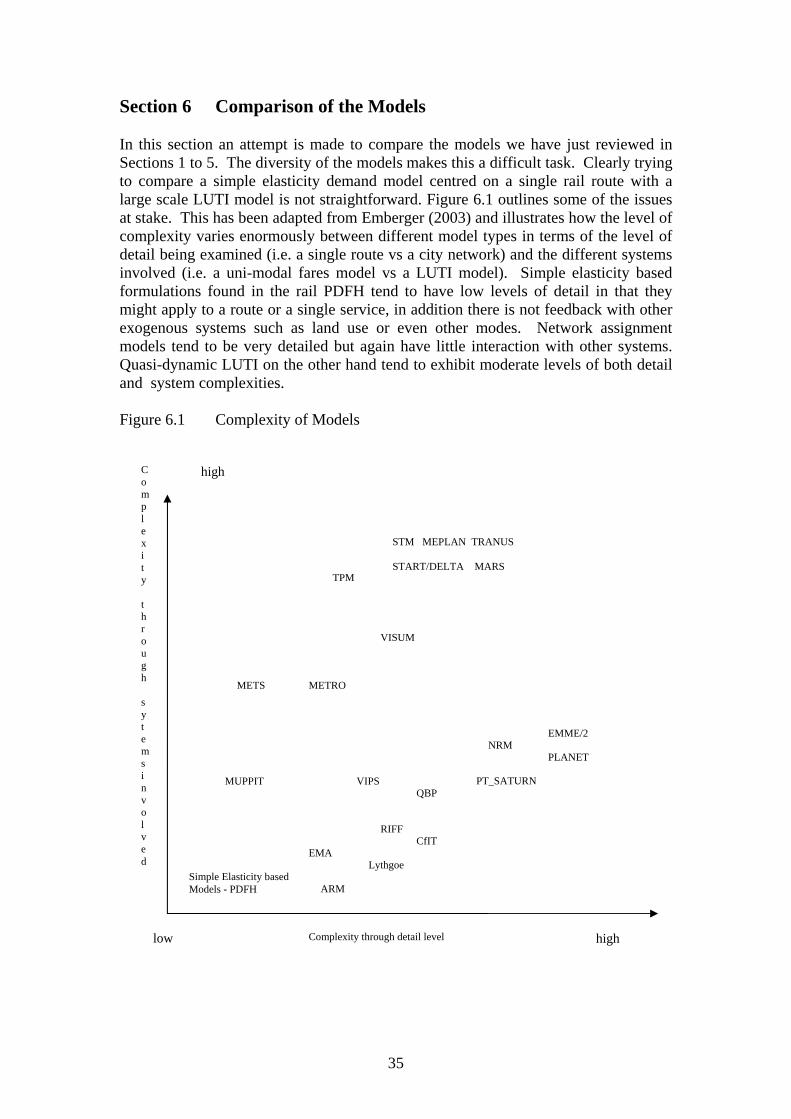
Section 6 Comparison of the Models In this section an attempt is made to compare the models we have just reviewed in Sections 1 to 5. The diversity of the models makes this a difficult task. Clearly trying to compare a simple elasticity demand model centred on a single rail route with a large scale LUTI model is not straightforward. Figure 6.1 outlines some of the issues at stake. This has been adapted from Emberger (2003) and illustrates how the level of complexity varies enormously between different model types in terms of the level of detail being examined (i.e. a single route vs a city network) and the different systems involved (i.e. a uni-modal fares model vs a LUTI model). Simple elasticity based formulations found in the rail PDFH tend to have low levels of detail in that they might apply to a route or a single service, in addition there is not feedback with other exogenous systems such as land use or even other modes. Network assignment models tend to be very detailed but again have little interaction with other systems. Quasi-dynamic LUTI on the other hand tend to exhibit moderate levels of both detail and system complexities. Figure 6.1 Complexity of Models

Complexity through sytems involved

high

STM MEPLAN TRANUS START/DELTA MARS

TPM

VISUM

METS METRO

low Complexity through detail level high

Simple Elasticity based Models - PDFH

PT_SATURN

RIFF

Lythgoe

NRM EMME/2

PLANET

EMA

MUPPIT VIPS QBP

CfIT

ARM

35

For any comparison to make some sense some simplifying assumptions are required. As a starting point let’s try to define some categories of policy instruments/influences which will impact upon the demand for public transport. In Table 6.1 these instruments/influences have been listed under five broad category headings which are deemed as appropriate to describe the impacts normally considered by models and modellers. At the same time it is recognised that some consistency is required between the policy instruments considered in Table 6.1 and those outlined in other sections of DISTILLATE. Therefore the policy instruments listed are matched (where possible) with those instruments outlined in the initial survey of local authorities carried out by DISTILLATE as part of work package The term ‘hard instruments’ relates to variables which are easily quantifiable and for which well established relations with demand are known. Public transport fare and service elasticities have been well researched and a series of empirical studies, based on both revealed and stated preference studies, has established accepted values. Similar research has been carried out for the main alternative, private car vehicles and also for cross demand effects between the two (TRL, 2004). Less is known about ‘soft instruments’ which are much harder to measure and whose value remains subjective to the traveller. Measuring the value placed upon ‘personal security’ or ‘cleanliness’ has relied on the use of stated preference techniques and the values are less well accepted in comparison to ‘hard values’. These values are however being seen as increasingly important by transport practitioners as they try to complete the picture on how travellers react to non-conventional public transport, i.e. rapid bus transport, park and ride, new information services etc. Both ‘hard’ and ‘soft’ instruments tend to be viewed as short term measures since they can be implemented with very short notice, although some instruments such as a new stations take several years to come on line their impact is felt immediately. The opposite applies to socio-economic, lifestyle and land use impacts which tend to be classified as medium to long term instruments/influences. For example, the performance of the economy can impact upon public transport demand via employment and disposable income levels; larger numbers of single person households may increase car ownership and lead to reductions in public transport demand; a move towards sustainable living may increase public transport demand; whilst a desire to save time by trip chaining may replace journeys previously undertaken by public transport with private car trips. Predicting the impact on public transport demand of such medium to long term influences is difficult, particularly so for certain measures such as a move towards sustainable living. It is not surprising then that the majority of the models reviewed in Sections One to Three have tended to concentrate on estimating the impact of ‘hard’ instruments on public transport demand. In order to facilitate a comparison of the models reviewed the report will now consider the models (section by section) and how they forecast changes in public transport demand in relation to the instruments/influences reviewed in Table 6.1. In doing so it is recognised that, whilst comprehensive, the number of instruments/influences outlined in Table 6.1 is not exhaustive. It is also acknowledged that underlying relationships exists between some of the instruments/influences that may affect their impact.

Table 6.1 Categories of Demand Policy Instruments/Influences Category Modelling Policy Instruments/Influences Distillate Policy Instruments Short Term a) Hard Instruments 1) Fares policy

2) Public transport frequencies 3) Public transport journey times 4) Public transport access/egress times 5) Public transport interchange times 6) Public transport reliability 7) Additional public transport services 8) New public transport services

• Fare levels • Fare structures such as flat fares, zonal fares and monthly passes • Concessionary fares • Integrated ticketing strateby • Changes in bus and rail frequencies • Timetabling strategies

• Bus priorities • On-bus cameras for traffic regulation enforcement • Timetabling strategies • Faster trains

• Pedestrian crossing facilities • Pedestrian routes • Pedestrian areas • New stations/stops • Terminal and interchanges

• Bus service measures to improve reliability • Bus priorities • Urban traffic control systems • Operational information systems such as bus fleet management • New bus services • New rail services on existing lines

• Light rail systems • Guided bus systems • Park and ride

9) Private car charges 10) Private car journey times & reliability

• Parking charges • Urban road charging • Vehicle ownership taxes • Fuel taxes • Conventional traffic management • Conventional speed controls • Urban traffic control systems • Intelligent transport systems • Accidental remedial measures • Traffic calming measures • New road construction • High occupancy car lanes

b) Soft Instruments 11) Quality of public transport ride 13) Quality of station/stop facilities 15) Passenger information 16) Quality of private car ride

• Real time information on board vehicles • Enhancement of bus and rail vehicles • Maintenance & cleanliness of bus and rail vehicles • On board personal security • Levels of overcrowding

• Maintenance & cleanliness • Personal security • Facilities • Lighting

• Real time passenger information at stops • Conventional timetable and other service information • Trip planning systems which provide information before the start of a

journey • Climate control, stereo system hands free phone etc. • Real time driver information systems and route guidance • Parking guidance and information systems

Medium to Long Term

38

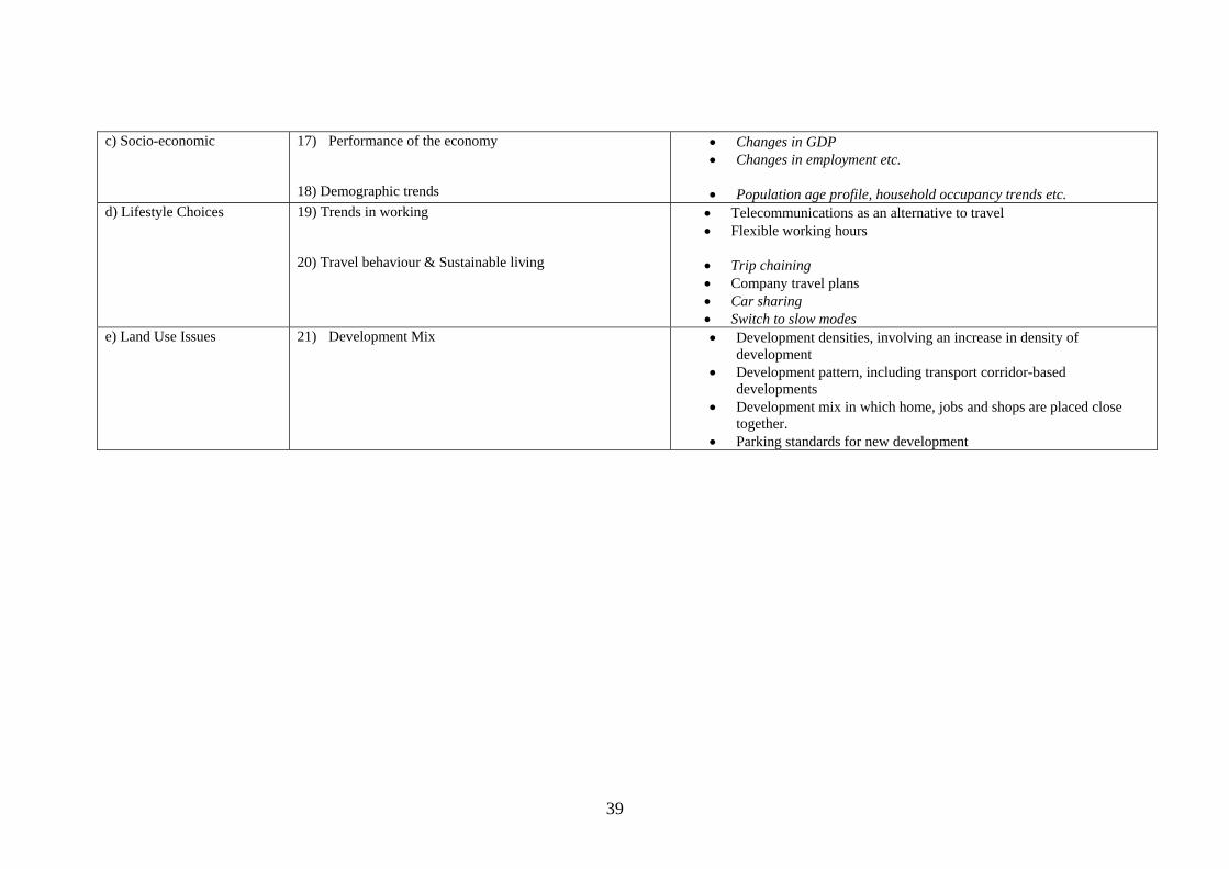
c) Socio-economic 17) Performance of the economy 18) Demographic trends

• Changes in GDP • Changes in employment etc.

• Population age profile, household occupancy trends etc.

d) Lifestyle Choices 19) Trends in working 20) Travel behaviour & Sustainable living

• Telecommunications as an alternative to travel • Flexible working hours • Trip chaining • Company travel plans • Car sharing • Switch to slow modes

e) Land Use Issues 21) Development Mix

• Development densities, involving an increase in density of development

• Development pattern, including transport corridor-based developments

• Development mix in which home, jobs and shops are placed close together.

• Parking standards for new development

39

6.1 Rail Models As the heading implies these models are uni-modal in nature and aim to predict changes in rail demand via factors that are both endogenous and extraneous to the rail market. That is not to say they don’t consider other modes, but when they do it is to assess how such competition affects the demand for rail and tends to be based on known diversion factors that can be implemented at a static rather than dynamic level. There is a mixture of static and dynamic analysis with the latter linked to LUTI models such as EMME/2. The majority of the models tend to concentrate on ‘hard’ instruments/influences and some also look at socio-economic instruments/influences with lifestyle and land use instruments/influences conspicuous by their absence (see Table 6.2). The PDFH is able to assess the impact on demand of a wide range of hard, soft and socio-economic factors, however each is in isolation of one another. The level of aggregation can vary between models as can the time scales. The variability in the latter will depend upon what policy or project is being assessed. If a train operator company wishes to know the impact of a change in the service frequency it offers it will only be interested in the short term implications of this. If on the other hand it is thinking about investing £0.5 billion in new rolling stock it will be interested in the medium to long term impact on rail demand. 6.2 Bus Models As with the rail models, the bus models are uni-modal in nature and aim to predict changes to bus demand via endogenous and extraneous factors. The ‘hard’ and ‘soft’ factors tend to predominate with no coverage of issues such as lifestyle and land use (see Table 6.3) instruments/influences. In recent years the ‘soft’ factors have received much more coverage and are increasingly seen as important elements in generating new demand and retaining existing demand. As with rail cross modal effects are considered in as much as how competition from other modes impacts upon bus demand and tends to take the form of modal diversion factors rather than dynamic interaction. The level of aggregation can vary between models, whilst in every case the time scales of the models are short. This might reflect the short term nature of the bus business and the flexibility of bus assets. The key aim for any bus operator is to make a short term profit, whilst for central and local government it is to keep within this and possibly next year’s budgetary constraints with regards support for bus services.. As such most of the modelling work tends to be short term in its outlook. Even when a major national bus company is making major investments in rolling stock, the flexibility of bus vehicles means that the risk can be spread out across the companies many regions, i.e. if buses aren’t required in Leeds then move them over to Leicester. 6.3 Simple Elasticity Recommendations These are somewhat different from the models we have reviewed elsewhere in this report in that they consist of a series of recommended elasticities for different impacts (changes in fares, service frequencies etc.) for different market segmentations (business travellers, leisure travellers etc.) at different levels of aggregation

(individual routes, county level, national level etc.). The PDFH covers the rail industry, the ARM the bus industry and the DfPT all public transport modes. 6.4 Multi-Modal Models As the title suggests these models examine more than one mode at the same time and perhaps more importantly cross modal effects on demand for each mode. This is not always as straightforward an example as say a cut in bus fares leading to a modal shift away from car. Higher car ownership may lead to a reduction in bus demand initially but then increased road congestion may see bus demand rise as traveller notice buses passing them in bus lanes. The interaction can be very complex especially for dynamic/quasi dynamic models that are based on a coded network carrying several modes to large numbers of O-D zones.

6.4.1 Road Traffic & Public Assignment Models All these models are based upon coded networks which will vary in coverage and detail, dependent upon the resources available to the transport practitioner using them. There appears to be quite good coverage of ‘hard’ instruments/influences and because all modes are coded onto the same network the interaction between the modes tends to be dynamic in nature. EMME/2 and VISUM appear to be able to model park and ride and other inter-modal trips which also allows them to examine trip chaining and activity analysis. EMME/2 also takes into account overcrowding levels on public transport but its not clear if this is simply a constraint on demand that can be carried or an input into the cost function (via additional vehicles). Unlike the bus and rail models overcrowding does not appear to be factored into any generalised cost function as a dis-benefit to the traveller. The major gaps appear to be the absence of ‘soft’, socio-economic and land use instruments/influences. In terms of time scale it would appear that all the models are interested in the short term impacts.

6.4.2 Micro-Simulation Models

Both STEER and DRACULA are involved in ongoing development as part of the DISTILLATE, with results reported as and when.

6.4.3 Demand Models The METS and MUPPET models can be viewed of more dynamic versions of the rail and bus models outlined earlier, with their focus being upon public transport demand but at the same time taking into account, in a dynamic fashion, the impact of private car vehicles. Whilst the METS model is highly aggregate, the MUPPET model is based upon a single corridor.

6.4.4 Land-Use/Transport Interaction (LUTI) & Strategic Demand Models All these models consider ‘hard’ instruments and the majority tend to consider socio-economic instruments/influences whilst two of them consider what are defined in Table 6.1 as land use influences. Both the STM and the START/DELTA models appear able to model new public transport infrastructure such as park and ride. It

41

42

appears that such new services are described in the same generalised cost terms as existing public transport services. As such they do not take into account some of the softer variables which are normally associated with them, i.e. low floor vehicles, the quality of the vehicles and ride. The overcrowding modelling that appears in the TPM and START/DELTA acts as both a constraint on demand and a dis-benefit to those travellers who experience them. All the models can based upon cities/regions but will differ in terms of O-D zone detail with the TPM model based upon 3 zones whilst the MARS model for Leeds can boast 33 O-D zones. In terms of time scale there is a tendency for this models to estimate long term affects, though the STM model appears to buck the trend and looks at short term impacts.

Table 6.2 Rail Models Policy Instruments/Influences Model Hard Soft Socio-economic Lifestyle Land Use

Level of Aggregation Time Scale

2.1 RIFF Yes: • Fare & Service changes • Cross modal impacts

No: Yes: • Population • Employment

No: No: Covers GB network using aggregate O-Ds. Able to disaggegate by trip purpose & ticket type.

Can be specified in terms of years.

2.2 Lythgoe Yes: • Fare & Service changes • New services • Access/egress times • Car impacts

Yes: • Regular interval

timetables

Yes: • Population

No: No: Covers GB network but can be estimated for any specific O-D pair.

Mainly short term estimating changes annually.

2.3 Praise Yes: • Fare & Service changes • Overcrowding • Cross modal impacts • Rail competition • Ticketing restrictions

No: No: No: No: Suited to individual rail routes or small networks.

Based upon daily changes.

2.4 NRM Yes: • Fare & Service changes • Cross modal impacts

No: No: No: No: Covers all national rail & London Underground stations, with very detailed zonal aggregation around Greater London and other large cities.

Strategic in nature so covers medium to long term.

2.5 PLANET Yes: • Fare & Service changes • New services • New Infrastructure • Cross modal impacts • Overcrowding

No: No: No: No: Based on north (1600 zones) and south (1400 zones) models for the morning and inter-peak time periods. Plus a smaller strategic all day model (250 zones).

Strategic in nature so covers medium to long term.

2.6 METRO Yes: • Fare & Service changes • New services • New PT infrastructure • Crowding • PT performance • Cross modal impacts

No: Yes:• Population; • GDP • Employment

No: No: Based on the W. Yorks PTE heavy rail network. Disaggregated down to route level.

Short –term looking at annual changes in PT demand.

43

Table 6.3 Bus Models Policy Instruments/Influences Model Hard Soft Socio-economic Lifestyle Land Use


3.1 EMA Yes: • Fare & service changes • Bus competition

No: No: No: No: Used to examine bus competition at a route level.

Short –term.

3.2 QBM Yes: • Fare & service changes • PT performance • Park and ride • Overcrowding • Bus competition • New services • Cross modal impacts

Yes: • Vehicle quality • Information • Low floor • Branding • Driver behaviour • Bus stop facilities • Cleanliness

No: No: No: Designed to accommodate bus networks of up to 50 stops; up to 5 operators; each offering up to 5 different ticket types; 2 market segments (concessions & non-concessions); and 4 time periods.

Short-term, usually for weekly periods.

3.3 CfIT Yes: • Fare & service changes • Overcrowding

Yes: • Vehicle quality • Information • Low floor • Branding • Driver behaviour • Bus stop facilities • Cleanliness

No: No: No: Designed to accommodate bus networks of up to 50 stops; 5 different ticket types; 2 market segments (concessions & non-concessions); and 4 time periods.

Short-term, usually for a year.

Table 6.4 Simple Elasticity Recommendations Policy Instruments/Influences Recommendations Hard Soft Socio-economic Lifestyle Land Use


1.1 PDFH Yes: • All + Cross modal

impacts

Yes: • All

Yes: • All

No: No: Varies from route level up to London, S. East & rest of the country. Able to disaggregate by trip purpose; ticket type; time/day of travel.

Mainly short term impacts.

1.2 ARM Yes: • All + cross modal

impacts

Yes: • All

Yes: • All

No: •

No:

Varies depending upon the transport practitioner. It can examine a single route or the whole aggregate UK data.

Short-term, usually monthly, 6 monthly & yearly.

1.3 DfPT Yes: • All + cross modal

impacts

Yes: • All

Yes: • All

No: • But provides

commentary

No:

Provides advice at various levels of disaggregation and for various trip purposes.

Various time scales.

44

Table 6.5 Multi-Modal Models Road Traffic & Public Transport Assignment Models Policy Instruments/Influences Model Hard Soft Socio-economic Lifestyle Land Use


4.1.a PT Saturn

Yes: • Fare & service changes • PT performance • Cross modal impacts

No: No: No: No: Dependent on the detail of the Saturn network that is coded. Short term

4.1.b EMME/2 Yes: • Fare & service changes • PT performance • Overcrowding • Park and ride • Cross modal impacts

No: No:

Yes: • Trip chaining

No: Dependent on the detail of the network that is coded in. Short term

4.1.c TRIPS Yes: • Fare & service changes • PT performance • Cross modal impacts

No: No:

No:

No: Dependent on the detail of the network that is coded in. Short term

4.1.d VIPS Yes: • Fare & service changes • PT performance • Cross modal impacts

Yes: • Information

No: No: No: Dependent on detail of coded network but typically based on a route level. Model can be specified for specific time periods.

Short term

4.1.e VISUM Yes: • Park and ride • Cross modal impacts

No: No: Yes:• Trip chaining

& activity analysis

No: Dependent on the detail of the coded network. Short term

Demand Models 4.3.a METS Yes:

• Fare & service changes • PT performance • Overcrowding • Cross modal impacts

No: No: No: No: Highly aggregate – Metropolitan level. Short term

4.3.b MUPPET

Yes: • Fare & service changes • PT performance • Cross modal impacts

No: No: No: No: Corridor based Short term

45

46

Table 6.5 Multi-Modal Models Land-Use/Transport Interaction (LUTI) & Strategic Demand Models Policy Instruments/Influences Model Hard Soft Socio-economic Lifestyle Land Use


4.4.a MEPLAN Yes: • Fares & service changes • New PT services • Cross-modal impacts • New PT infrastructure • New roads • Road charging • Parking costs

No: Yes: • Population • Employment • GDP

No: Yes: City/Region:Numer of O-D zones is dependent upon the transport practitioner, i.e. Helsinki Area model covers 81 zones and an area of 14,400 kms2

Demand can be split by mode, trip purpose and time of day.

Long Term

4.4.b TRANUS Yes: • Fares & service changes • New PT services • Cross-modal impacts • New PT infrastructure • New roads • Road charging • Parking costs

No: Yes:• Population • Employment • GDP

No: Yes: City/Region:Number of O-D zones & network links is dependent upon the modeller, i.e. the Brussels model has the Brussels-Captial Region and 116 municipalities in the suburbs. Demand can be split by mode, trip purpose and time of day.

4.4c TPM Yes: • Fare & service changes • Overcrowding • Cross-modal impacts

No: Yes:• Population • Employment

No: No: Town or city wide level of aggregation comprising 3 zones – models exist for various UK cities including Bristol, Edinburgh & Leeds. Can model 8 modes of transport, 8 journey purposes, 3 car ownership categories and t time periods per day.

Long term

4.4.d MARS Yes: • Fares & service changes • New PT services • PT performance • Cross-modal impacts

No Yes:• Population • Employment

No: Yes: Town/City. Number of O-D zones depends on transport practitioner, i.e. Leeds has around 33 zones). Demand can be split by mode, trip purpose and time of day.

Long term

4.4.e START/DELTA

Yes: • Fares & service changes • New PT infrastructure • PT performance • Cross-modal impacts • Overcrowding

No: Yes:• Population • Employment • GDP

No: Yes City/region.Transport demand varies by time of day, mode and route.

Long term

4.4.f STM Yes: • Fare & service changes • PT infrastructure – park and

ride, LRT, new rail stations • Cross-modal impacts

No: No: No: No: Town/city/regional wide level of aggregation – models exist for various UK cities including Gloucester and Reading. Number of zones dependent upon transport practitioner.

Short term

6.5 Gaps in Research In this section of the report a number of gaps in the current research are identified and expanded upon. They relate to a need and a desire to improve current modelling methods. Some may be beyond the scope of the DISTILLATE research remit but are listed anyway. It is apparent that certain impacts are under-represented in all types of models, most prominently ‘lifestyle’ impacts. It also becomes apparent that the gaps which appear in some models may be closed by including an approach from another modelling area, for example by including rail demand modelling in multi-modal models. 6.5.1 General Gaps (a) Lifestyle Impacts Lifestyle impacts tend to be under-represented in all types of public transport models. They cover developing trends in modern day working, travel behaviour and sustainable living. These can give rise to the use of telecommunications as an alternative to travel; flexible working hours; trip chaining, company travel plans, car sharing and a switch towards slow modes. As yet the majority of public transport models have failed to take into account lifestyle impacts and it is not difficult to see why. It is difficult to predict when a commuter may decide to work at home instead of travelling into the office. Even when they do make that decision will they work at home 1 day a week or 2 days a week or 3 days per week? Similar problems exist when trying to model car share or company travel plans, however, with the latest estimates suggesting that 7.5% of the UK’s population did some form of teleworking during 2003, a figure that had doubled from 1997 (ONS, 2005). The impact of lifestyle changes is becoming increasing important and cannot be ignored. (b) Soft Variables Other impacts which can sometimes be under-represented in public transport models are those discerning to ‘soft’ variables. Impacts which come under these heading relate to variables which are difficult to measure and to value. Examples include, the quality of the PT ride (levels of personal security, cleanliness of bus and rail vehicles, levels of overcrowding…); the quality of the PT station/stop facility (personal security, facilities, lighting …); passenger information (real time information at stops, pre-journey information….); and the quality of the private car ride (climate control, route guidance systems…). Recently there has been a great deal of valuation work which has improved our understanding of how important such variables are to passengers/potential passengers, however such values have been slow to filter through to public transport models and is an issue that needs addressing. 6.5.2 Rail Models

(a) Improving Cross Modal Impacts - A number of the rail models make an attempt to take into account cross modal impact via static diversion factors and elasticities. This leads to static analysis and mis-estimation of impacts if the data or underlying assumptions about the relationships is inherently wrong. There is a need to introduce some dynamics into the cross modal

47

relationships by testing out policies not related to rail but to other modes of transport, i.e. private car or bus.

(b) Inclusion of Soft Variables - The majority of the models don’t take into

account ‘soft’ instruments such as rolling stock quality. There is a need to take into account their impact upon demand.

(c) Introducing Social-Economic Impacts - In most of the models these

impacts are provided as static exogenous factors. There is a need to make these endogenous to the model or link them to another model which can provide some dynamism to the analysis.

(d) Introducing Lifestyle Influences - To date there has been no research that

has examined the impacts on rail demand of lifestyle influences such as trip chaining, sustainable living etc.

(e) Land Use Influences – There appears to be little consideration of land use

influences. There may be scope here for some cross pollination of ideas between existing land use models and more specific rail based models.

6.5.3 Bus Models

(a) Long Term Impacts – A need to consider demand impacts over the longer term including the inclusion of socio-economic, lifestyle and land use instruments/influences.

(b) Bus Rapid Transit (BRT) – Examine the impacts of such schemes on bus demand.

(c) Lifestyle Influences – What are the impacts of trip-chaining, sustainable living etc.

6.5.4 Multi-modal Models 6.5.4.1 Road Traffic & Public Transport Assignment Models

(a) Improvement of demand models – By the inclusion of the impacts from ‘soft’ variables.

(b) New PT Modes – Examine impact of quality bus routes and BRT. (c) Lifestyle Influences – What are the impacts of trip-chaining, sustainable

living etc. 6.5.4.2 Micro Simulation Models Ongoing development 6.5.4.3 Demand Models See discussion for rail and bus models. 6.5.4.4 LUTI Models

(a) Improved Specification - Of public transport demand and supply functions/parameters, particularly for soft variables and new public

48

transport infrastructure and modes such as heavy rail, quality bus routes, park and ride and BRT. There could be scope here for some cross-pollination of ideas with existing rail and bus demand models.

(b) Lifestyle Influences – What are the impacts of trip-chaining, sustainable living etc.

49

Section 7 The Way Forward in Distillate In this section the report proposes a number of possible case studies which will attempt to plug the gaps in the research identified in section 6.4 and will form the basis of the next phase of the Distillate project In choosing possible case studies a number of factors have to be considered in order to arise at a decision as to whether the case study is feasible. Are there enough resources to carry the case studies through to completion? Does the data exist? If we are to use an existing model can we access it? How does this fit into the needs outlined by local authorities? After discussion between the ITS team members a number of possible case studies are outlined below which are felt to feasible under the Distillate remit. 7.1 PT-Saturn & Quality Bus Case Studies The aim of this case study would be to introduce quality bus into PT-Saturn. There is a growing body of evidence from the bus industry examining the values placed upon the characteristics of quality bus and how they are best represented in demand functions. PT-Saturn is owned by AS Atkins and is a suite of programs designed to complement the traffic modelling suite SATURN and, in this respect, is capable of modelling:

• The choice between public and private transport modes; • Route choice in both public and private modes; • The choice of where to travel (now or later/earlier); • The choice of switching destination.

Initial discussions with Atkins, who developed the PT-Saturn module have been encouraging and we understand that a small network covering Harrogate would be made available to us. In addition they would be make resources available to us to make modifications and improvements (such as adding in quality bus) to the model. Our approach will look at importing the Quality Bus parameter values from ITS’s existing Quality Bus Model. There may also be scope for using the results in the general SATURN model. 7.2 MARS Case Studies We have identified a number of possible case studies based around MARS. These are listed below and would help improve the specification of public transport demand and supply functions/parameters within MARS, particularly for soft variables and new public transport infrastructure and modes such as heavy rail, quality bus routes, park and ride and BRT. The model has already been coded up for the Leeds network and would be available.

• A public transport over-crowding model – The issue of overcrowding is increasingly becoming an important for urban rail and bus services. To date MARS has not dealt with the issue specifically and there would be scope for its introduction. ITS’s experience in modelling over-crowding and we would be looking at importing some of that experience into the MARS model.

50

• Soft variables – Are not well represented in MARS. Introducing behavioural impacts via public transport reliability, branding, safety and security would be an advancement.

• Heavy rail link – A two way link between MARS and the METRO rail model would address a number of the issues outlined in sections 6.4. The supply data from the METRO model could be used to incorporate heavy rail links into the Leeds MARS model and then the demand from the O-D zones calibrated. This would allow the impact of car based policies on heavy rail demand to be tested and vice-versa. The link could also work the other way and provide the METRO model with socio-economic inputs such as population changes over time. This would allow the METRO model to extent its current impact assessment from short run impacts to long run impacts.

7.3 METRO Heavy Rail Model

As well as linking up with the MARS model there are a number of improvements that could be made to the existing METRO model particularly to the modal split procedure which is currently based on static elasticities taken from the PDFH. Apart from the proposed link up with the MARS model focus will be on implemented a logit based choice model within the existing METRO model. 7.4 DRACULA Case Studies Recent work has imported public transport routes from PT-SATURN and it’s our intention to build upon this by looking at the dynamic modelling of public transport users’ route choice and the effect of modelling capacity of bus routes. This will be conducted as a theoretical exercise using a hypothetical network to allow us to develop the algorithms. 7.5 STEER Case Studies The proposed work will see us investigate which measures are best at improving bus journey times within urban settings without unduly penalising cars. A range of instruments will be considered along with what the optimal combination of methods are? The measures include:

• bridge closures to car traffic, • bus priority measures through bus lanes and signals, • bus design, route and frequency changes, and • network management schemes for both car and slow modes.

7.6 STM Case Studies This case study will see the Strathclyde STM used to develop better techniques for sketch modelling of modal interchange using data from the Scottish Household Survey and outputs from the large scale network model SITM4 (Strathclyde Integrated Transport Model).

51

References:

Abraham, J.E. and Hunt, J.D. (1999) “Policy Analysis Using the Sacramento MEPLAN Land Use Transportation Interaction Model”. TRB Conference.

Batty, M (1976): Urban modelling. Cambridge University Press, Cambridge. De la Barra T (1989): Integrated Land Use and Transport Modelling. Cambridge University Press, Cambridge.

Bristow, A.L., Mackie, P.J., Preston J.M., Whelan, G.A., Huang B and Shires, J.D. (2002) “Achieving Best Value for Public Support of the Bus Industry: Part 1. Summary Report on the Modelling and Assessment of Seven Corridors”. A Report for CfIT. http://www.cfit.gov.uk/research/psbi/lek/pdf/appendix9.pdf

Centre for Economics & Business Research (1998) “Rail Forecasts for the West End & City”. Report for the Passenger Demand Forecasting Subscription Service. Clegg, R.G., Ghali, M.O., Smith, M.J.(1995), “Equilibrium/Control results and the approach to a near-equilibrium of a new Dynamic Micro-simulation/Assignment model on a Network Model of York”. Applications of Advanced Technologies in Transportation Engineering, Published by the American Society of Civil Engineers, pp568-572. Citilabs (2005) – TRIPS Model – www.citilabs.com/trips/ David Simmonds and Marcial Echenique & Partners Ltd (1999) “Review of Land-use/Transport Interaction Models & Reviews”. Report to the Standing Advisory Committee on Trunk Road Assessment. DETR. www.roads.dft.gov.uk/roadnetwork/sactra/support99/index.htm Department for Transport (1982) “Urban Public Transport Subsidies & Economic Assessment of Value for Money”/ Technical Report, DfT. London. Department for Transport (2005a) “WEBTAG”. www.webtag.org.uk Department for Transport (2005b) “TAG Unit 1.1 Introduction to Transport Analysis”. www.webtag.org.uk/webdocuments/1_Overview/1_Introduction_to_Transport_analysis/index.htm Department for Transport (2005c) “TAG Unit 2.1 The Overall Approach: Steps in the Process”. www.webtag.org.uk/webdocuments/2_Project_Manager/1_Overall_Approach_Steps/index.htm

Department for Transport (2005d) “TAG Unit 2.4 Summary Advice on Modelling”. www.webtag.org.uk/webdocuments/2_Project_Manager/4_Summary_Advice_on_Modelling/index.htm

52

http://www.cfit.gov.uk/research/psbi/lek/pdf/appendix9.pdf

http://www.citilabs.com/trips/

http://www.roads.dft.gov.uk/roadnetwork/sactra/support99/index.htm

http://www.webtag.org.uk/







Department for Transport (2005e) “TAG Unit 3.1.2 Transport Models”. www.webtag.org.uk/webdocuments/3_Expert/1_Modelling/3.1.2.htm

Department for Transport (2005f) “TAG Unit 3.1.3 Land Use/Transport Interaction Models”. www.webtag.org.uk/webdocuments/3_Expert/1_Modelling/3.1.3.htm

Department for Transport (2005.g) – National Rail Model - www.dft.gov.uk/stellent/groups/dft_econappr/documents/page/dft_econappr_610405-07.hcsp Department for Transport (2005.h) – National Transport Model – www.dft.gov.uk/stellent/groups/dft_econappr/documents/divisionhomepage/030708.hcsp Dodgson, J., Katsoulacos, Y.S. and Newton, C. (1993) “Application of the Economic Modeling Approach to the Identification of Predation” Journal of Transport Economics and Policy, May 1993. Emberger, G. (2003) “Local Transport Plans Guidance: Forecasting & Appraisal”. Task 3 Report to the Department for Transport. Institute for Transport Studies, University of Leeds. Friedrich, M. (1998) “A Multi-Modal Transport Model for Integrated Planning”. 8th World Conference of Transport Research. Antwerp. Institute for Transport Studies (2003) “Area Review Model Handbook”. A Confidential Report for First Group. INRO (2005) – EMME/2 - www.inro.ca/en/products/emme2/index.phpJMP Consultants Ltd (2004) “Rail in the City Regions: Report to PTEG”. Johnson, D.H. and Nash, C.A. (2005) “Charging for Scarce Capacity: A Case Study of Britain’s East Coast Mainline”. Third Rail Conference on Railroad Industry Structure, Competition and Investment. Marcial Echenique & Partners Ltd (1992) “Technical Introduction to MEPLAN”. Cambridge. Modelistica (2005) – TRANUS Model - www.modelistica.com/tranus_english.htm Liu, R. (2005), The DRACULA dynamic network microsimulation model. In: Kitamura, R. Kuwahara, M. (Eds), Simulation Approaches in Transportation Analysis: Recent Advances and Challenges, Springer, pp23-56. Lythgoe, W.F. and Wardman, M. (2004) “Modelling Passenger Demand for Parkway Rail Stations”. Transportation 31, pp. 125-151. Office for National Statistics (2005) “UK Labour Force Survey.” Office for National Statistics, UK Government.

53



http://www.dft.gov.uk/stellent/groups/dft_econappr/documents/page/dft_econappr_610405-07.hcsp

http://www.dft.gov.uk/stellent/groups/dft_econappr/documents/page/dft_econappr_610405-07.hcsp

http://www.dft.gov.uk/stellent/groups/dft_econappr/documents/divisionhomepage/030708.hcsp

http://www.dft.gov.uk/stellent/groups/dft_econappr/documents/divisionhomepage/030708.hcsp

http://www.inro.ca/en/products/emme2/index.php

http://www.modelistica.com/tranus_english.htm

Ortuzar, J. and Willumsen, L. (2001) “Modelling Transport”. 3rd Edition, John Wiley & Sons Ltd. Passenger Demand Forecasting Council (2002) “Passenger Demand Forecasting Handbook”. 4th Edition. Pfaffenbichler, P. and Shepherd, S.P. (2003) “A Dynamic Model to Appraise Strategic Land-use and Transport Policies.” European Journal of Transport and Infrastructure Research. Special Issue: Sustainable Transport. Volume 2 Issue 3/4. pp 255-283. (2003). Preston, J., Nash, C.A. and Toner, J. (1993) “MUPPIT: Urban Transport Market Theoretical Analysis”. ITS, University of Leeds, Working Paper 412. PTV AG (2005) – VIPS Model – www.ptv-scandinavia.se/vips PTV AG (2005a) – VISUM Model – www.ptvag.com/cgi-bin/traffic/traf_visum.pl Simmonds, D C and B G Still (1998) “DELTA/START: Adding Land Use Analysis to Integrated Transport Models”. World Conference on Transport Research 1998. Steer Davies Gleave (1999) “Rail Industry Forecasting Framework”. Prepared for Association of Train Operating Companies & Railtrack, London. STRATEC (2004) “Simulations With Integrated Land-use/Transport Models in 3 Case Cities: Brussels, Helsinki & Stuttgart. An Assessment of the Impacts of the Simulated Measures”. Deliverables 5 & 6 of SCATTER (Sprawling Cities & Transpot: from Evaluation to Recommendations). www.casa.ucl.ac.uk/scatter/download/D5_D6_scatter_part1.pdf Strategic Rail Authority (2002) – PLANET Suite of Models: www.sra.gov.uk/news/2002/12/sra_announces_new_transport_forecasting_ TRL (2004) “The Demand for Public Transport: A Practical Guide”. TRL Report, TRL593. TRL (2005) – TPM (Transport Policy Model) - www.trlsoftware.co.uk/index.asp?Section=Products&Item=TPM TRL (2005a) – STM (Strategic Transport Model) – www.trlsoftware.co.uk/index.asp?Section=Products&Item=STM Van Vliet, D. (1982) “SATURN – A Modern Assignment Model”. Traffic Engineering and Control, 23, pp 578-581. Wardrop, J.G. (1952) “Some Theoretical Aspects of Road Traffic Research”. Proceedings of the Institution of Civil Engineers, Part II 1, 325-362.

54

http://www.ptv-scandinavia.se/vips

http://www.ptvag.com/cgi-bin/traffic/traf_visum.pl

http://www.casa.ucl.ac.uk/scatter/download/D5_D6_scatter_part1.pdf

http://www.sra.gov.uk/news/2002/12/sra_announces_new_transport_forecasting_

http://www.trlsoftware.co.uk/index.asp?Section=Products&Item=TPM

http://www.trlsoftware.co.uk/index.asp?Section=Products&Item=STM

Whelan, G. and Johnson, D.H. (2004) “Modelling the Impact of Alternative Fares Structures on Rail Overcrowding”. International Journal of Transport Management, Vol. 2, pp. 39-46. Whelan, G.A., Toner, J.P., Mackie, P.J. and Preston, J.M. (2001) “Modelling Quality Bus Partnerships”. 9th World Conference on Transport Research, Seoul, Korea. Whelan, G., Preston, J., Wardman, M. and Nash, C.A. (1998) “The Privatisation of Passenger Rail Services in Great Britain: An Evaluation of Competition for the Market and Competition in the Market”. Proceedings of the 8th World Conference on Transport Research. WS Akins (2000) “PT SATURN: A Users Guide”. www.its.leeds.ac.uk/software/saturn/downloads/PT-SATURN%20Manual.DOC

55

http://www.its.leeds.ac.uk/software/saturn/downloads/PT-SATURN Manual.DOC

appendix b review of public transport models f appendix b.pdf · review of public transport models...

Documents