A26 - 1

Appendix 26 Stabilizing Measures of the Navigation Channel

Appendix 26.1 Unsteady flow riverbed change analysis using Two-Dimensional

Flow Model

In this Study, the Study Team proposes to predict changes in the unsteady flow

riverbed using numerical simulations as a means of evaluating appropriate

measures for navigable waterway maintenance and sedimentation control in the

Red River, an inland waterway artery through the metropolitan area of Hanoi City,

capital of the People’s Republic of Vietnam.

For the river sections covered by the predictions, computations will be made for

unsteady flow riverbed changes using a two-dimensional flow model to evaluate

the impacts of low water channel dike improvement, pier construction and

dredging of navigable waterways on the riverbed.

1. Outline of prediction model

1.1 Basic equation for Two-dimensional Unsteady Flow Model (Cylindrical

Coordinates System)

The basic equations for flow regime and sediment transport have been obtained.

(1) Basic equation for two-dimensional shallow water flow model (flow regime)

The basic equation for two-dimensional shallow water flow model in the

cylindrical coordinates system is given as indicated below.

<Equation of motion>

2222

1vuu

Ksg

nu

nsu

shs

sp

ruv

nu

vsu

utu

+−

∂∂

∂∂

+

∂∂

∂∂

+−∂∂

−=+∂∂

+∂∂

+∂∂

εερτ

ρ・ ....(1)

222

2

21

vuvKs

gnv

nsv

shnp

ru

nv

vsv

utv

+−

∂∂

∂∂

+

∂∂

∂∂

+−∂∂

−=+∂∂

+∂∂

+∂∂

εερτ

ηρ・ .....(2)

<Equation of continuity>

( ) ( )

01

=∂

∂+

∂∂

+∂∂

nrvh

rsuh

th

・ ....(3)

where;

s, n: distances in downstream direction and transverse direction,

respectively,

A26 - 2

u,v: average flow velocity in directions of s and n, respectively,

h: water depth,

p: water pressure,

ρ: density of fluid,

r: radius of curvature,

τs, τn: riverbed shear force in directions of s and n, respectively; the

Manning formula is used,

ε: turbulent eddy viscosity,

g: gravitational acceleration,

κ: Karman’s constant (=0.4),

u*: frictional velocity,

Ks: permeability coefficient of trees,

nm: Manning roughness coefficient

22

34

2

vuuh

gnhs m +=

ρτ

....(4)

22

34

2

vuvh

gnhn m +=

ρτ

....(5)

hu*1κ

ε = ....(6)

(2) Basic equation for sediment transport

<Equation of motion for bed load>

• Equation for sediment transport in downstream direction (Meyer-Peter-Muller

equation )

( ) ( ) 5.1**

3 '1/8 csBS gdq ττρρ −−= ・ ....(7)

• Equation for sediment transport in transverse direction (Hasegawa’s

equation)

( )( ) nzuvqq ksCbbBSBn ∂∂−= /// ** ・τµµτ ....(8)

where;

qBS: sediment transport per unit width in direction of axis s

ρs: density of gravel

ρ: density of running water

d: particle size of riverbed material

τ?: dimensionless effective shear force

A26 - 3

τ*c: dimensionless critical shear force

qBn: sediment transport per unit width in direction of axis n

vb/ub: flow direction on riverbed

τ*: dimensionless shear force

μs:static friction coefficient

μk: dynamic friction coefficient

<Equation of motion for suspended sediment>

• Equation of continuity for suspended particles

( ) ( ) ( )hCwqnC

hDns

ChD

srhvC

nrhuC

su

tC

h bfsuns −+

∂∂

∂∂

+

∂∂

∂∂

=∂∂

+∂∂

+∂∂

・1

....(9)

• Equation for amount of floating suspended particles (Itakura-Kishi equation)

( ) ( )

−−

Ω=

− gd

WK

gd

q

s

f

ss

su

1/'1/ **

ρρτρρ

αρρ

・ ....(10)

( )

( )1

'

exp1

exp1

'

0*

*

'

2

'

2

*

* −+−

−=Ω

∫

∫∞

∞

ητ

αξξπ

αξξπ

ξτ

BBa

a ,

0*

* 1'

'ητ

−=B

a ....(11)

where C: density of suspended sediment

Ds: diffusion coefficient in direction of axis s

Dn: diffusion coefficient in direction of axis n

qsu: amount of floating suspended particles from riverbed

Wf: sedimentation velocity of suspended particles

Cb: density of suspended particles near riverbed

η0: 0.5

B*:= 0.143

α*:=0.14

K: =0.008

<Equation of continuity>

( ) 01

11

=

−+

∂∂

+∂

∂−

+∂∂

bfsuBnBs CWqn

qrs

qtZ

・λ

....(12)

where Z: height of riverbed

t: time

λ: void ratio of riverbed material

A26 - 4

2. Flow chart for simulation analysis of unsteady flow riverbed changes

Figure A26.1.1 shows the flowchart of steps in simulation analysis of unsteady flow

riverbed changes. Brief descriptions for the individual steps are given below.

2-1 Objective and description of computations

The basic policy for the simulation analysis will be drawn up on the basis of

examination of the computation conditions and outputs and will be established

after discussions with the Vietnamese authorities. The basic policy will also be

confirmed by consultation with the Vietnamese side after the preliminary

computations using simplified topographic model referred to later have been

made.

All the materials and data necessary for establishing the basic policy for simulation

analysis are as listed below.

(1) Data relating to building topographic model

• Plan, longitudinal profile and lateral profile of the area covered by computations

• Plan and lateral profile of improvement plan

• Data on riverbed height

• Data on trees and vegetation inside river channel

(2) Data on boundary conditions for water levels and discharge

• Water levels (downstream end) and discharge data (upstream end and lateral

inflow) during past floods and longitudinal flood mark water level data (for model

verification)

• Water level data (downstream end) and discharge data (upstream end and

lateral inflow) during other floods considered

(3) Other data

• Survey data on riverbed material

• Field measurements of suspended sediment density and data on relations with

river discharge

• Survey data on riverbed roughness

A26 - 5

2-2 Computation output

• Calculated water level (values and contour map)

• Flow velocity (vector diagram)

• Riverbed height (values and contour map)

2-3 Analysis with Simplified Topographic Model (preliminary computation)

Numerical simulations of unsteady flow riverbed changes normally involve a great

deal of computations and thus it does not always prove efficient to undertake

computations using full-scale topographic model (detailed model) from the outset.

For this reason, the Study Team proposes to make preliminary computations using a

simplified topographic model and to study the conditions for use in the

computations with the detailed topographic model. After this process the

analytical method and policy will be verified.

2-4 Production of topographic model

The area covered by the analytical computations will be divided into appropriate

mesh grids and X-Y coordinate values will be determined. The division into mesh

grids will be made on the basis of the data listed below.

• Configuration of low water channel and high water channel alignment

• Survey lines for lateral profile of river

• Planning of river structures

The next step is to determine the ground levels for the topographic model. When a

lateral profile of the river is available, the dividing positions in the transverse

direction will be projected on the lateral profile and their elevations will be taken as

the ground levels. When the lateral profile is not available, the ground levels will be

determined using a topographic plan.

2-5 Establishment of boundary conditions

The necessary boundary conditions will be established in the manners described

below.

A26 - 6

(1) Boundary conditions for water level and discharge

The boundary conditions for discharge and water level will be established at the

upstream end and downstream end, respectively, on the basis of actual

measurements.

(2) Roughness and resistance coefficients

The roughness coefficient for the riverbed will be established taking account of the

river channel conditions and previous relevant studies, while the resistance

coefficient will be established where the river channel is clustered with trees and

other plants. The values of these coefficients will be determined after the model

reproducibility of the actual flow regime is verified.

(3) Boundary conditions for particle size of riverbed material

The boundary conditions for the particle size of riverbed material will be established

on the basis of the survey data on riverbed material.

(4) Boundary conditions for inflow material at upstream end

The boundary conditions for inflow material at the upstream end will be established

after

performing sediment load capacity computations for one-dimensional non-uniform

flow or unsteady flow on the basis of field suspended sediment measurements and

riverbed material survey data. These conditions will be corroborated by the

outcome of riverbed change computations for movable beds.

2-6 Reproducibility computations for actual flow regime

Under the fixed bed conditions which do not consider changes in the riverbed,

reproducibility computations for flood marks will be undertaken using the water

level and discharge data pertaining to previous floods to evaluate the

appropriateness of necessary parameters such as the model topography and

roughness and resistance coefficients.

2-7 Reproducibility computations for actualities with movable bed

Computations for riverbed changes will be performed with a movable bed taken

into consideration to evaluate the model reproducibility of actualities. Where these

A26 - 7

computations indicate stability of the actual river channel or changes with time in

the longitudinal and lateral profiles, analysis will be undertaken to determine if the

computation results agree with the trends of the actual changes.

2-8 Computations for prediction of future flow regime and riverbed change

Simulations of riverbed changes will be carried out using a combination of

discharge conditions and structural conditions of the plan.

2-9 Collation of computation results

The computation results will be collated and compiled into charts and diagrams.

The computation results for the actual conditions and those for predicting future

conditions will be compared to evaluate the changes in riverbed height and

effectiveness of proposed improvement measures. The outputs will include

comparison tables and charts, flow velocity vector diagrams, and water level

contour maps.

3. Grid Arrangement

The Grid s for simulation calculations are arranged as shown in Figure A26.1.2.

A26 - 8

Figure A26.1.1 Flowchart of Steps in Prediction of Riverbed Changes in the Red

① Establish Work Schedule - Confirm Study Items - Establish Study Policy

② Study by Simplified Topographic Model - Build Simplified Topographic Model - Verify Methodology for Study and Policy - Determine Computation

③ Construction of Full-Scale Topographic Model - Divide into Mesh Grids - Determine Ground Height

⑤ Computation of Reproduction of Actual Flow Regime - For Dry Season - for Rainy Season

⑥ Establishment of Boundary Conditions (Riverbed Changes) - Conditions of Riverbed Materials - Conditions of Inflow Materials at Upstream End

⑦ Study on Reproducibility of Riverbed Changes - For Dry Season - For Rainy Season

⑧ Simulation Analysis of Riverbed Changes - With Measures for Navigation Channel Stabilization - For Short-term Development Plan

⑨ Collation and Compilation of Computation Results - Compare and Collate Computation Results - Compile into Maps, Charts and Diagrams

⑩ Evaluation

(Changes etc. of Study Method )

< Computation of Reproduction of Actual Flow Regime >

< Computation for Prediction of Riverbed Changes >

< Preparation of Prediction Model >

④ Establishment of Boundary Conditions (Flow Regime) - Conditions of Water Level and Discharge - Roughness, Coefficient of

A26 - 9

N

Fig

ure

A26

.1.2

G

rids

Arr

an

ge

me

nts

A26 - 10

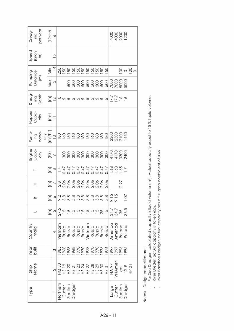
Ap

pe

nd

ix 2

6.2

Tab

le A

26.2

.1

Dre

dg

ing

Fle

et o

f Vie

t Na

m W

ate

rwa

y C

on

stru

ctio

n C

oo

pe

ratio

n (

VIN

AW

AC

O)

Ty

pe

Sh

ip

Na

me

Ye

ar

bu

ilt

Co

un

try

ma

id

L B

H

T En

gin

e

Ca

pa

-c

ity

Pum

p-

ing

c

ap

a-

city

Ho

pp

er

Ca

pa

- c

ity

Dre

dg

-in

g

De

pth

Pum

pin

g

Dis

tan

ce

(m

)

Spe

ed

(k

no

t/

hr)

Dre

dg

- in

g

pe

r ye

ar

(m)

(m)

(m)

(m)

(PS)

(m

3 /h

r)

(m3 )

(m

) M

ax

Min

(103

.m3 )

1

2

3 4

5

6 7

8 9

10

11

12

13

14

15

16

Suc

tion

D

red

ge

r Lo

ng

C

ha

n

Tra

n H

D

ao

H

B 38

1969

19

69

1989

Ge

rma

ny

Ge

rma

ny

Vie

tna

m

95

95

53.7

16

16

10

6 6 4

5.3

5.38

1.

6

5810

66

50

1590

3500

35

00

400

3,20

0 3

,500

.. 40

0

16

16

7

10

10

7

3500

35

00

500

Sea

Ba

ckh

oe

D

red

ge

r

TC81

TC

82

TC54

TC

91

1981

19

82

1954

19

89

Fra

nc

e

Fra

nc

e

Ge

rma

ny

Ru

ssia

69.8

69

.8

52.5

12.6

12

.6

9.73

4 4 3.3

2.4

2.4

1.85

2060

20

60

665

920

800

800

300

600

16

16

14

14

10

10

4-5

1000

10

00

300

300

Riv

er

Dre

dg

er

TC 8

2 19

83

Ru

ssia

52

.6

9.6

2.8

1.8

490

275

12

250

Cu

tte

r Se

ctio

n

Dre

dg

er

H 0

1 H

02

H 0

3 H

04

H 1

9/5

Pe

Ka

6

H 0

6

1961

19

65

1965

19

65

1982

19

75

1965

Am

eric

a

Am

eric

a

Am

eric

a

Am

eric

a

Vie

tna

m

H.L

A

me

rica

39

21

21

21

25

24

23

11

8.

8 8 8.

33

7.08

7.

4

2.8

2.5

1.5

1.8

2.2

1.8

3.2

2.1

1.0

1.0

1.0

1.2

1.2

1.2

1950

11

85

1185

11

85

1065

17

00

910

500

480

480

480

480

500

300

10

10

10

10

10

10

9.

5

2000

15

00

1500

15

00

1500

50

00

1200

200

200

200

200

200

300

200

30

0 20

0 30

0 30

0 55

0

Sou

the

rn

Cu

tte

r Se

ctio

n

Dre

dg

er

H 0

6 H

07

H 0

8 H

09

H 1

0 H

11

H 1

2 H

22/

12

H 3

0/4

1986

19

85

1963

19

64

1965

19

65

1979

19

84

1985

Vie

tna

m

Vie

tna

m

Am

eric

a

Am

eric

a

Am

eric

a

Am

eric

a

Vie

tna

m

Vie

tna

m

Vie

tna

m

19

16

15

15

15

15

16.5

16

.5

6.

6 6.

5 5.

5 5.

5 5.

6 6.

2 3.

75

3.75

1.

8 1.

6 1.

6 1.

6 1.

25

1.5

1.2

1.2

1.

0 0.

85

1.05

1.

05

1.0

0.9

0.8

0.8

525

545

574

574

574

290

375

215

215

250

300

300

300

300

100

200

100

100

8 8 8 8 5 8 5 5

80

0 80

0 80

0 10

00

500

500

300

300

20

0 20

0 20

0 20

0 10

0 15

0 10

0 10

0

A26 - 11

Typ

e

Ship

N

am

e

Yea

r b

uilt

C

ou

ntr

y m

aid

L

B H

T En

gin

e

Ca

pa

-c

ity

Pum

p-

ing

c

ap

a-

city

Ho

pp

er

Ca

pa

- c

ity

Dre

dg

-in

g

De

pth

Pum

pin

g

Dis

tan

ce

(m

)

Spe

ed

(k

no

t/

hr)

Dre

dg

- in

g

pe

r ye

ar

(m)

(m)

(m)

(m)

(PS)

(m

3 /h

r)

(m3 )

(m

) M

ax

Min

(103

.m3 )

1

2

3 4

5

6 7

8 9

10

11

12

13

14

15

16

No

rth

ern

C

utt

er

Suc

tion

D

red

ge

r

HQ

30

HS

19

HS

20

HS

21

HS

23

HS

24

HS

27

HS

28

HS

29

HS

30

HS

31

1985

19

68

1968

19

68

1970

19

70

1978

19

70

1970

19

76

1976

Vie

tna

m

Ru

ssia

R

uss

ia

Ru

ssia

R

uss

ia

Ru

ssia

V

ietn

am

R

uss

ia

Ru

ssia

R

uss

ia

Ru

ssia

27.5

15

15

15

15

15

15

15

15

25

15

9.2

5.8

5.8

5.8

5.8

5.8

5.8

5.8

5.8

5.8

5.8

2.8

2.06

2.

06

2.06

2.

06

2.06

2.

06

2.06

2.

06

2.06

2.

06

1.4

0.47

0.

47

0.47

0.

47

0.47

0.

47

0.47

0.

47

0.47

0.

47

30

0 30

0 30

0 30

0 30

0 30

0 30

0 30

0 30

0 30

0

180

160

160

160

180

180

160

160

180

180

180

10

5 5 5 5 5 5 5 5 5 5

50

0 50

0 50

0 50

0 50

0 50

0 50

0 50

0 50

0

250

150

150

150

150

150

150

150

150

150

150

Larg

e

Cu

tte

r Su

ctio

n

Dre

dg

er

HA

97

VN

Am

eri

ca

12

-9

HP

01

1997

19

97

1996

19

95

Am

eric

a

Am

eric

a

Po

lan

d

Po

lan

d

34.7

34

.7

35

36.5

9.15

9.

15

1.

07

2.

97

1.68

1.

68

1.65

1.

7

4170

41

70

3300

24

00

2300

23

00

2100

14

50

17

.7

17.7

16

16

7000

70

00

5000

50

00

10

0 0 100 0

40

00

4000

20

00

1200

No

tes)

D

esi

gn

ca

pa

citi

es

are

: -

For

Sea

Dre

dg

er,

ca

lcu

late

d c

ap

ac

ity is

liq

uid

vo

lum

e (

m3 )

. Ac

tua

l ca

pa

city

eq

ua

l to

15

% li

qu

id v

olu

me

. -

Riv

er

Dre

de

r, a

ctu

al c

ap

ac

ity is

ta

ken

65%

. -

Riv

er

Bac

kho

e D

red

ge

r, a

ctu

al c

ap

ac

ity h

as

a f

ull

gra

b c

oe

ffic

ien

t o

f 0.

65.

A26 - 12

Appendix 26.3 Conditions of Numerical Simulations

A26.3.1 Boundary Conditions related to Currents

1.1 Dry Season Results of the surveys in January 2002 are applied to the calculations. Water level at Hanoi Station is set as 3.11m. Water levels at the lower boundary (No. 10) and the Duong River (No.5) are first given based on the measured levels. Then, the water discharge at the upper boundary(No.1) is assumed based on Statistical Analysis Results on Hydrological Data.

Table A26.3.1 Boundary Conditions (Dry Season)

Location Water level (m)

Discharge(m3/s)

Remarks

No.1 (4.44) 1,750 Upper end No.5 3.39 (510) Duong River

No.10 2.34 (1,240) Lower end

1.2 Flood Season Results of the surveys in August 2002 are applied to the calculations. Water level at Hanoi Station is set as 9.33m. Water levels at the lower boundary and the Duong River are given based on the measured levels. Then, the water discharge at the upper boundary is assumed based on Statistical Analysis Results on Hydrological Data.

Table A26.3.2 Boundary Conditions (Flood Season)

Location Water level (m)

Discharge(m3/s)

Remarks

No.1 (10.30) 10,445 Upper end No.5 9.33 (3,265) Duong River

No.10 8.18 (7,180) Lower end

1.3 Very High Flood Data at Hanoi and Truong Cat Stations in August 2002 are applied to the calculations. Water level at Hanoi Station is set as 12.50m.

A26 - 13

Figure A26.3.1 Locations of Boundaries Water levels at the lower boundary (No. 10) and the Duong River (No.5) are first assumed based on the above analysis for the Flood Season. Then, the water discharge at the upper boundary is assumed based on Statistical Analysis Results on Hydrological Data.

Table A26.3.3 Boundary Conditions (Very High Flood)

Location Water level (m)

Discharge(m3/s)

Remarks

No.1 (14.08) 22,715 Upper end

No.5 13.05 (7,254) Duong River

No.10 11.50 (15,461) Lower end

Upper Boundary

Duong River

Lower Boundary

No.10

No.5

No.1

A26 - 14

1.4 Extremely High Flood Water level is assumed as 13.4ｍ at Hanoi Station. Referring to the H-Q diagram based on observed data from 1957 to2000, water levels at the Duong River and the lower boundary are estimated. Water discharge at the upper boundary is calculated by adding water discharges at the Duong River and the lower boundary. It is assumed that there is no breakdown of the dikes.

Table A26.3.4 Boundary Conditions (Extremely High Flood)

Location Water level (m)

Discharge(m3/s)

Remarks

No.1 (14.8) 32,381 Upper end No.5 13.5 (10,381), Duong River

No.10 12.5 (22,000) Lower end

A26 - 15

A26.3.2 Conditions on Riverbed Materials

2.1 Roughness Coefficients

Roughness coefficients are determined referring to the LANDSAT image shown below in Figure A26.3.1. Basically it is considered that the roughness condition is different among lower channel, sand bar, and floodplain: Lower channel: 0.025

Sand bar: 0.030 for bars with small grain size, bars relatively newly created, and places where color is white on the LANDSAT image.

Floodplain: 0.040 for bars with vegetation and resident areas

Figure A26.3.1 LANDSAT Image of the Red River, Hanoi Segment

A26 - 16

2.2 Grain Size Distribution Conditions of riverbed materials is formulated based on the results of laboratory tests of grain size distribution done in January 2002. According to the cumulative distribution curves, the grain size distribution is different between the lower river channel and the floodplain (including sand bars). Deviation of each distribution is small as shown in Figure A26.3.2. Therefore, the distribution is classified into two patterns. Table A26.3.5 shows division of size, median diameter and composition of each size.

0

20

40

60

80

100

1 10 100 1000 10000

Size(microns)

Perc

enta

ge u

nde

rsiz

e(%

)

Surface Ave.

0.5m Below Surface Ave.

Surface Ave.(sandbar)

0.5m Below Surface Ave.(sandbar)

Figure A26.3.2 Grain Size Distributions of Bed Materials

A26 - 17

Table A26.3.5 Conditions of Particle Size of Bed Materials

Code of particle size

Division of size (micron)

Median

diameter (micron)

Average composition in the lower

channel (Cumulative %)

Average composition in sand bars

(Cumulative %)

D01 5000.0 ～ 10000.0 7500.00 100.00 100.00 D02 2000.0 ～ 5000.0 3500.00 99.88 100.00 D03 1000.0 ～ 2000.0 1500.00 99.47 99.99 D04 500.0 ～ 1000.0 750.00 98.18 99.60 D05 355.0 ～ 500.0 427.50 94.50 99.31 D06 250.0 ～ 355.0 302.50 85.26 98.53 D07 180.0 ～ 250.0 215.00 69.51 96.32 D08 125.0 ～ 180.0 152.50 38.23 91.57 D09 90.0 ～ 125.0 107.50 19.07 82.83 D10 63.0 ～ 90.0 76.50 6.17 64.60 D11 44.2 ～ 63.0 53.60 60.28 D12 31.2 ～ 44.2 37.70 55.64 D13 22.1 ～ 31.2 26.65 49.78 D14 15.6 ～ 22.1 18.85 43.02 D15 11.0 ～ 15.6 13.30 36.55 D16 7.8 ～ 11.0 9.40 30.39 D17 5.5 ～ 7.8 6.65 24.95 D18 3.9 ～ 5.5 4.70 20.47 D19 2.76 ～ 3.9 3.33 16.56 D20 ～ 1.95 0.98 13.38