APPENDICES

1950s photographs were classified by Pierce et al. as Woody Shrub. We assume that neither authors had this type present; pre-channelization distribution is assumed to be zero. Ludwigia spp. were also mentioned as possible invaders of Floating Tussocks by Milleson et al. Our Ludwigia spp. floating mat shrubland (S.LSF) and Miscellaneous floating mat shrubland (S.MxFS) both possibly could be linked with Floating Tussock in Milleson et al. However, because shrub-dominated mats were not mentioned by either authors, both are assumed to have had zero distribution in the pre-channelization floodplain.

Wet Depression (DW). This category was defined by Pierce et al. as a circular area within drier habitats having “distinctive vegetation zonation” in response to deeper water toward the center of the depression. The zones they describe, however, seem adequately described by other of their categories, e.g., SJ (Hypericum fasciculatum) and PS (Broadleaf marsh). We have not linked with this category.

Submergent vegetation (no Pierce et al. category). Submergent and floating aquatic communities other than floating mats were not defined by Pierce et al. or Milleson et al., except by such categories as Open Water (below).

Other Categories

Cultivated (CU). We have no areas currently under cultivation in Pool C and have not defined a cultivated category.

Open Water categories (KR. OW. and OX ). Pierce et al. did not treat submergent or surface vegetation in their classification, so we consider these categories unvegetated at the time of their air photos. Milleson et al. did not separately define (nonmarsh) aquatic vegetation types, so our No vegetation - open water (NVOW) category is not fully comparable to their OW (they included in their OW vegetation that we are separating from our NVOW because of the presence of submergent vegetation). Milleson et al. definition: “Generally deep water areas which are devoid of vegetation; however, some shallow water areas may have submergent species such as southern naiad (Najas guadalupensis) and eel grass (Vallisneria americana).” Pierce et al.’s and Milleson et al.’s categories are linked with our NVOW.

Svoil and Natural Levee (.SP, LR). Vegetated spoil will be mapped as the dominant vegetation, as was done in Pierce et al. Milleson et al. includes a Vegetated Spoil category that includes vegetation that we have linked with our Miscellaneous invasive herbaceous vegetation (H.MxW) category. Milleson et al. definitions: “Spoil And Levees: Large, barren piles of sand, shell, and limerock deposited alongside C-38 from the dredging operation; water control and/or access levees; and service roads” (many of these areas are currently vegetated); “Vegetated Spoil: Portions of the spoil piles colonized by vegetation such as natal grass (Rhychelytrum repens), broomsedges (Andropogon sp.), and thistles (Cirsium horridulum)

Human-influenced (CU. CA, AP, CN, SR). Included in Pierce et al.’s classification Cultivated, Cultivated Abandoned, Artificial Ponds, Canals, and State Roads. “Urban” in Milleson et al. Milleson et al. is defined as: “A land use classification which includes commercial fish camps, resort and residential areas, locktender residences, and water control structures.” All are linked with our No vegetation - human- made structures (NVH) category.

A-78

APPENDICES

Glossary of terms used in the baseline vegetation classification.

baseline vegetation classification or new baseline vegetation classification: the classification presented in this document.

baseline: the post-channelization, pre-restoration condition of the Kissimmee River and floodplain.

bcode: abbreviation for the community type level in the baseline vegetation classification. For example, “MC” is the bcode for Myrica cerifera shrubland. Bcodes can be prefixed by physiognomic qualifiers to denote forest (F), shrub (S), or herbaceous (FI) community types (e.g., “S.MC”).

category: generic term used to describe groupings at any hierarchical level of any classification.

community type: term for the finest level of the KRREP baseline vegetation classification, to which bcodes apply. Comparable to the terms “vegetation type” or “association” used in other classifications (e.g. Myrica cerifera shrubland).

decision rules: rules for distinguishing between alternative choices. In this classification, decision rules are organized in the Key to Community Types.

dominant: as used in the Key, the species or physiognomic group with greatest cover.

gradients: areas where vegetation is transitioning from one community type to another, and is therefore difficult to characterize. Gradient vegetation is handled in the Key by use of combination codes (e.g., H.PS-PH vegetation).

heterogeneous polygon: a polygon that contains more than one distinct community type (by our decision rules) in patches that are greater than the minimum mapping unit (MMU).

initial baseline vegetation classification: the prior baseline vegetation classification developed for Pool C vegetation mapping during 1996-1999.

KRREP: Kissimmee River Restoration Evaluation Program.

linkage: equivalence of categories in different classifications.

MMU: minimum mapping unit = 10x10 m or 100 square meters on the ground; appx. 1.67 x 1.67 mm (0.067 x 0.067 in.) on Pool C 1996 aerial photography, assuming the nominal photo scale of 1:6000.

mosaic: a polygon that contains two distinct community types (by our definitions), one of which occurs in a more or less regular distribution of below-MMU patches.

physiognomic group: upper level of the baseline vegetation classification in which vegetation is subdivided by dominant physiognomy, e.g., forest, shrubland, or herbaceous vegetation.

previous classifications: the vegetation classifications used by Pierce et al. (1982) and Milleson et al. (1980) in their vegetation maps.

APPENDIX 9-3A

A-79

APPENDICES

Species codes used in the classification.

APPENDIX 9-4A

Code SpeciesAA01 Ambrosia artemisiifoliaAA02 Amaranthus australisAA05 Ampelopsis arboreaAC01 Axonopus compressusAC02 Azolla carolinianaAC10 Aster carolinianusAD01 Symphyotrichum dumosumAD01 Aster dumosusAE01 Aster elliottiAE02 Symphyotrichum elliottiiAF01 AxonopusfurcatusAF02 Axonopus fissifoliusAF02 Axonopus affinisAG01 Acalypha gracilensAG05 Andropogon glome ratusAI01 Asclepias incamata

AM01 Amphicarpum muhlenbergianumAM99 Amaranthus sp.AP01 Altemanthera philoxeroidesAR01 Acer rubrumAS01 Amaranthus spinosusAV01 Andropogon virginicusAX99 Axonopus sp.BC01 Bacopa carolinianaBC05 Boehmeria cylindricaBC99 Bacopa sp.BD01 Boltonia diffusaBH01 Baccharis halimifoliaBL01 Bidens laevisBM01 Bacopa monnieriBM02 Bidens mitisBS01 Blechnum serrulatumCA01 Centella asiaticaCA05 Cyperus articulatusCA11 Carex alataCA15 Callicarpa americanaCC01 Cuphea carthagenensisCC02 Conoclinium coelestinumCC03 Cyperus croceusCC04 Cyperus compressusCD01 Ceratophyllum demersumCDOls Ceratophyllum demersumCD05 Commelina diffusa

Code SpeciesCD05s Commelina diffusa_________C D10 Cynodon dactylonC D 2 5 Cyperus distinctusCE01 Cyperus erythrorhizosCF01 ComusfoeminaCF02 CannaflaccidaC GO 1 Commelina gigasCHOI Cyperus haspanCH05 Cirsium horridulumCH99 Chara sp.CJ01 Cladium jamaicenseCL 01 Carex longiiCL02 Cyperus lanceolatusCL03 Coreopsis leavenworthiiCM01 Cardiospermwn microcarpumCN05 Chamaecrista nictitansCOOl Cephalanthus occidentalisCOOS Cyperus odoratusCP00 Cyperaceae sp.CP01 Cyperus polystachyosC P 9 9 Cyperus sp.CR01 Cyperus retrorsusCR99 Cary a sp.CS01 Cyperus surinamensisCS99 Cirsium sp.CT01 Ceratopteris thalictroidesCT99 Citrus sp._________________CV01 Cyperus virensCV02 Carex vexansCX99 Carex sp.DC01 Drymaria cordataDC02 Digitaria ciliaris___________DC03 Dichondra caroliniensisDE01 Dichanthelium erectifoliumDG99 Digitaria sp.DI01 Desmodium incanumDL01 Digitaria longiflora_________DP03 Digitaria pentziiDS01 Digitaria serotinaDS99 Desmodium sp.DT01 Desmodium triflorumDV01 Diodia virginiana__________DV02 Decodon verticillatus

A-80

APPENDICES

APPENDIX 9-4 AContinued

Code SpeciesDV05 Diospyros virginianaEB01 Eragrostis bahiensisEB02 Eryngiim baldwiniiEC01 Eichhomia crassipesEC05 Eupatorium capillifoliumEC10 Eleocharis cellulosaEC15 Euthamia carolinianaEE01 Eragrostis elliottiEF01 EleocharisflavescensEG01 Eucalyptus grandisEH01 Erechtites hieraciifoliaEI01 Eleocharis interstinctaEI05 Eleusine indicaEL01 Eragrostis lugensEL99 Eleocharis sp.EOOl Eleocharis olivaceaEQ01 Erigeron quercifoliusER99 Eragrostis sp.EV01 Eleocharis viviparaEVOls Eleocharis viviparaEWOl Echinochloa walteriFAOl Fimbristylis autumnalisFCOl Fraxinus carolinianaFC02 Fimbristylis carolinianaFDOl Fimbristylis dichotomaFM99 Fimbristylis sp.FPOl Fuirena pumilaGCOl Geranium carolinianumGTOl Galium tinctoriumGUOl Galium uniflorumHAOl Hemarthria altissimaHA02 Hyptis alataHA15 Hymenachne amplexicaulisHC02 Hypericum cistifoliumHFOl HypericumfasciculatumHGOl Hibiscus grandiflorusHHOl Hypericum hypercoidesHMOl Hypericum mutilumHP99 Hypericum sp.HROl Habenaria repensHR05 Hydrocotyle ranunculoidesHTOl Hypericum tetrapetalumHUOl Hydrocotyle umbellataHU02 Hedyotis uniflora

Code SpeciesHU02 Hedyotis unifloraHV01 Hydrilla verticillataIA01 Ipomea albaIC01 Ilex cassineIC02 Imperata cylindricaIG01 Ilex glabraIP99 Ipomea sp.IS01 Ipomea sagittataIV01 Iris virginicaJA01 Justicia angustaJE01 Juncus effususJM01 Juncus marginatusJNOO JUNCACEAEJN99 Juncus sp.KB01 Kyllinga brevifoliaKOOl Kyllinga odoratus (odorata?)KP01 Kyllinga pumilaKV01 Kosteletzkya virginicaLA01 Lythrum alatumLC01 Lantana camaraLC05 Lachnanthes carolinianaLD01 Ludwigia decurrensLD02 Lindemia dubia var. anagallideaLD99 Ludwigia sp.LF01 Hydrochloa caroliniensisLF01 Luziola fluitansLH01 Leer si a hexandraLL01 Ludwigia leptocarpaLM01 Lygodium microphyllumLM02 Ludwigia maritimaLM99 Lemna sp.LP01 Ludwigia peruvianaLR05 Ludwigia repensLS01 Ludwigia suffructicosaLS02 Limnobium spongiaLV01 Lepidium virginicumMA01 Myriophyllum aquaticumMC01 Myrica ceriferaMC02 Momordica charantiaML01 Macroptilium lathyroidesMP01 Mitreola petiolataMP05 Melothria pendulaMS01 Mikania scandensMU01 Micranthemum umbrosum

A-81

APPENDICES

APPENDIX 9-4 AContinued.

Code SpeciesMV01 Magnolia virginianaNG01 Najas guadalupensisNL01 Nuphar luteaNS01 Nyssa sylvatica (var. biflora)OCOl Osmunda cinnamomeaOC02 Oxalis comiculataOROl Osmunda regalisOS99 Osmunda sp.PA01 Paspalum acuminatumPA02 Panicum ancepsPA03 Panicum angustifoliumPA04 Phragmites australisPA05 Phytolacca americanaPA99 Passiflora sp.PB01 Persea borboniaPCOO POACEAEPC01 Pontederia cordataPC01 Pontederia lanceolataPC02 Ptilimnium capillaceumPC05 Paspalum conjugatumPC99 Pluchea sp.PD01 Polygonum densiflorumPD02 Paspalum dissectumPD04 Panicum dichotomumPD06 Paspalum dilatatumPD11 Paspalum distichumPE01 Pinus elliottiPERIs PeriphytonPF01 Paspalum floridanumPF02 Pluchea foetidaPG01 Psidium guajavaPG05 Paspalidium geminatumPH01 Panicum hemitomonPH05 Polygonum hirsutumPHI 0 Polygonum hydropiperoidesPH20 Panicum hiansPLOl Paspalum laevePL99 Polygonum sp.PNOl Paspalum notatumPNIO Phyla nodifloraPN99 Panicum sp.POOl Pluchea odorataPPOl Polygonum punctatumPP02 Proserpinaca palustris

Code SpeciesPP02s Proserpinaca palustrisPP03 Polypremum procumbensPP04 Persea palustrisPP07 Physalis pubescensPQ01 Parthenocissus quinquefoliaPR01 Panicum repensPR02 Panicum rigidulumPROS Pluchea roseaPR10 Paspalum repensPS01 Pistia stratiotesPS02 Paspalum setaceumPS03 Panicum sphaerocarponPS05 Peltandra sagittifoliaPU01 Paspalum urvilleiPV01 Panicum verrucosumQL01 Quercus laurifoliaQN01 Quercus nigraQR99 Quercus sp.QV01 Quercus virginianaRC01 Rubus cuneifoliusRC02 Rhynchospora colorataRC03 Rhus copallinumRC05 Rhynchospora cephalanthaRC10 Rhynchospora chalarocephalaRD01 Rhynchospora decurrensRF01 RhynchosporafascicularisRI01 Rhynchospora inundata

RM01 Rhynchospora microcarpaRM05 Rhexia marianaRM10 Rhynchospora microcephalaRN01 Ricciocarpus natansRN05 Psilocarya nitensRN05 Rhynchospora nitensRN99 Rhynchospora sp.RS01 Richardia scabraSA01 Sisyrinchium angustifoliumSA02 Sida acutaSA04 Smilax auriculataSA06 Solanum americanumSB01 Spartina bakeriSC01 Salix carolinianaSC02 Sida cordifoliaSC05 Scirpus cubensisSC10 Sarcostemma clausum

A-82

APPENDICES

APPENDIX 9-4 AContinued.

Code Species Code SpeciesSC15 Sambucus canadensis SV05 Sesbania sp.SC20 Scirpus califomicus SZ01 Sphenoclea zeylanicaSC25 Saururus cemuus SZ01 Sphenoclea zeylanicaSC99 Scirpus sp. TC01 Teucrium canadenseSD01 Scoparia dulcis TD01 Taxodium distichumSD99 Sida sp. TD02 Thelypteris dentataSE01 Sida elliottii TD05 Typha domingensisSF01 Solidago fistulosa TG01 Thalia geniculataSI01 Sacciolepis indica TI01 Thelypteris interruptaSI02 Sporobolus indicus TK01 Thelypteris kunthiiSL01 Sagittaria lancifolia TL01 Typha latifoliaSL02 Smilax laurifolia TL99 Thelypteris sp.SL05 Sagittaria latifolia TN99 Tillandsia sp.SL99 Solanum sp. TP01 The lypte ris palustrisSM01 Salvinia minima TR01 Trifolium repensSM05 Suriana maritima TV01 Triadenum virginicumSM10 Setaria magna UC01 Urtica chamaedryoides

SMILAX Smilax sp. UL01 Urena lobataSN99 Senna sp. UM01 Brachiaria mutica (synonym)SOOl Cassia obtusifolia UM01 Urochloa muticaSOOl Senna obtusifolia US01 Urochloa subquadriparaS002 Senna occidentalis UT99 Utricularia sp.SPOO SPARGAN1A CEAE VA01 Vicia acutifoliaSP01 Sabal palmetto VL01 Vigna luteolaSP02 Setaria parviflora VL02 Viola lanceolataSP99 Sphagnum sp. VR01 Vitis rotundifoliaSR01 Serenoa repens VS01 Verbena scabraSR02 Sida rhombifolia VS02 Vigna speciosaSR05 Smilax rotundifolia VT99 Vitis sp.SR10 Scleria reticularis WA01 Woodwardia areolataSS01 Sacciolepis striata WD99 Woodwardia sp.ST01 Schinus terebinthifolius WG01 Woljffiella gladiataST99 Setaria sp. WV01 Woodwardia virginicaSV01 Solanum viarum XF01 XyrisfimbriataSV02 Sesbania vesicaria XR99 Xyris sp.SV03 Senecio vulgaris

A-83

APPENDICES

APPENDIX 9-5A

T able o f linkage w ith p revious K issim m ee R iver vegetation classifications. C ategory and h ierarchy term ino logy for the p rev ious classifications are from P ierce et al. (1982), T ab le 9-1 and M illeson et al. (1980), T able 9-1.

Cells m arked' .... " have no equivalent in the classification indicated. These community types arc assumed to have had zero distribution at the time o f that classification®.linkage w ith categories in parentheses was assumed

S ee Append ix 3 fu r a d iscussion o f linkage w ith the P ierce e l al. MP category' M illeson et. al d id tint, list, the Soft. Rush Depression typo in thoir T nhlo I; it. is included h rrn hconnnr: it. if; m entioned in the text, o f th e ir docum crlio th the hassling c lassification and the P irtre e t.n l document, c lassify vegetation on spoil piles and

1 The Wet Depression type found in Pierce et al. will be mapped by vegetation present

bcode Com m unity Type Fhysiojpom y W etland/ Upland H abitat bcodeppup

bcode group name P icrc cc ta l (1982) code(<) Fierce et al. (1982) category PicrccctaL(1982)

upper categoryMilleson ct al. (1980)

categoryMilleson ct al. (1980) upper

category

FAR Acer rubwm (-Nyssa silvatica var. bitlora) forest

Forest. Wetland WF Wetland Forest. (MP)1 (Wetland hardwood forcst)l Forested wetland Hardwood trees Wetland forested

I1' I 'd l-raximis caroliniana forest. Konst. Wetland Wl'' Wetland forest. (MP)1 (Wetland hardwood forest)l forested wetland 1 lardwood trees Wetland forested1- M'lT' Mixed transitional forest. forest Wet,land WK Wetland 1''orest. — — — —

F.MV Magnolia virginiana forest Forest Wetland WF Welland Forest ..... —

F.MxF Miscellaneous upland forest Forest Upland UF Upland Forest — — — —

F.PE Pmus ellidhi loresl Forest Upland UF Upland Forest PP Pme Forest Nalive upland — —

vqn Quercus virginiana (-Sabalpalmetto'; forest horest. Upland ill' Upland forest. OK Oak/Cabbage Palm Native upland Oak and cabbage palm Terrestrial forested

F.SP Sabal palmetto forest Forest Upland UF Upland Forest OK Oak/C abb age Palm Native upland Oak and cabbage palm Terrestrial forestedI'.TL) Taxodium distichum forest l-orest Wetland WP Wetland i-'crest a Cypress i-'orest Porested wetland Cypress Wetland forested

H.AF Axonopus fissifolius herbaceous vegetation Hcrbaccous Upland UP Upland Hcrbaccous n Improved Pasture Human influcnccd Improved Pasture Agriculture and urban

H.AGAndi’opogyji gloineralus heibaceous

vegetation Hcrbaccous Wetland WT' Wet rTairic (WP) (Wet Prairie) Emergent wetland . . . . . .

H.CD Cynodon dadylon heibaceous vegetation

Herbaceous Upland UP Upland Herbaceous

H C J Cladiuin jamaiceaise heibaceous vegetation

Herbaceous Wetland MW Miscellaneous Welland Vegetation

a Sawgrass Eineigenl wetland Saw grass M arJi

H.CS Cypeius spp. heibaceous vegetation Herbaceous Wetland W W elPraine (WP) (Wei Prairie) EinergenlW dland —

H.EC Eichliorma crassipes herbaceous aquatic vegetation Herbaceous Wetland A Q Aquatic Vegetation FM Floating Mat Aquatic Floating tussocks Marsh

H.EC PST Eidihcrnia crassipes-Pistia stratiotes herbaceous aquatic vegetation Herbaceous Wetland AQ Aquatic Vegetation FM Floating M ai Aqualic Floating lussods Marsh

H.ES Eleodiaris spp. heibaceous vegetation Herbaceous Wetland WP Wet Prairie (WP) (Wet Prairie) Emergent Wetland

H.HA Hemarthria altissima herbaceous vegetation Herbaceous Upland UP Upland Herbaceous

H.HG Hibiscus grand itlorus herbaceous vegetation Herbaceous Wetland BLM Broadleal'Mai'sli PS Broadleal'Mai’sli Emergent Welland Bivadleal'Marsh Marsh

H.HU Hydnscctle umbellata heibaceous aquatic vegetation Herbaceous Wetland AQ Aquatic Vegetation — . . . . -

IIIV Iris virginica herbaceous vegetation 1 lerhaceoiis Wetland WP Wet. Prairie (WP) (Wet. Prairie) Kmergent. Wetland —

H JE d JUncus effusus herbaceous vegetation (upland depressions) Herbaceous Wetland WP W et Prairie (WP) (Wet Prairie) Emergent Wetland Soft rush depression2 Marsh

H.JEpJuncus ellusus herbaceous

vegetation (wet prairies) Herbaceous Wetland WP Wet Prairie (WP) (Wet Prairie) Emergent Wetland Soft rush pond Marsh

H.LF Luzicda tluitans herbaceous vegetation

Herbaceous Wetland WP Wet Prairie WP Wet Prairie . . . .

111,11 Leersia hexandra herbaceous vegetation

1 lerhaceoiis Wetland WP Wet. Prairie (WP) (Wet. Prairie) (Kmergent Wetland) (Aquatic (irasses) Marsh

H M FM Miscellaneous heibaceous floating mat. vegetation Hcrbaccous Wetland AQ Aquatic Vegctntion FM Floating Mat. Aquatic Floating tussodrs Marsh

H M xE Miscellaneous exotic herbaceous vegetation Heibaceous Upland UP Upland Herbaceous (Vegetated Spoil) (Spoil and Barren)

H M xFA Miscellaneous aquatic vegetation dominated by floating species Herbaceous Wetland AQ Aqualic Vegdalion - .... —

HJMadFNMiscellaneous fem -dominated

herbaceous vegetation Herbaceous Wetland MWMiscellaneousWetJand

Vegetaticn — . . . . . . . . — . . .

H M xM Miscellaneous littoral marsh vegetation Hcrbaccous Wetland AQ Aquatic Vegetation ..... . . . . . . . .

HLMEN Miscellaneous native herbaceous vegetation Herbaceous Upland UP Upland Herbaceous PU Unimproved Pasture Human Influenced Unimproved Pasture Agriculture and Urban

HMxSVMiscellaneous submergent aquatic

vegetation Herbaceous Wetland AQ Aqualic Vegdalion (US) (Unknown-submerged) (Miscellaneous) —

HMxW Miscellaneous invasive herbaceous vegetation Herbaceous Upland UP Upland Herbaceous PU Unimproved Pasture Human Influenced Unimproved Pasture,

(Vegetated Spoil)Agriculture and Urban, (}!poi

and Bairtai)

A-84

APPENDICES

APPENDIX 9-5A

C ontinued,

Invdc Cuiuiiuuft'i ftyVNpKNIlJ \\ rtUuO VplMUO HvtbJUl bci»deomip lnwlC|(ivM iniiw PlrrceriuLflnG)

todefi)PlfKCCtBiaiW)upk« cmninr

MJllnun A uL (UWl oMoinr

MlUrwii n ul (MW) uppn auijjiy

HMxWP MiMxK«i«ujxl(;«nijuullwi»6k*Atf WJtUlVd Kdmoecuc Wdlnd WP WdPluiRc m (Wctftur?) EnMf<sLWcUmd

HMtWT Miscdlimcuj nitnr* HhUiuma W<Uanl WP WttPiimm

HKL Ntytaf lixai htAttwm igatiffvty iLui HulriWM WdboJ AQ A'ju — .... — ... —

HML Nuyloi lut« llVlt<f.V.V« 4'14l4V TTiriwxaa WtUad Atjmiv: Vtjriialinsi - .... - . .. -

HIV htfKvAUK «|Witio VftMtfltion HaUvvw. W«tUud AQ k'pit. Wy&AvM — .... — ... —

IlH i Paniaim heflvtanm hataeeous v«pU bui UvbKcau W<tiJDd WP w prurw MC Mai<3<ncn«W<Fnine LmefA<ntW«]ttd MuteKiMWttPnn* llXSl

HW Flip iliu nvUtun tnrti v«eUtx HertacwiK Upland UP UptifwlHcfbaim'. Pt IrrififWPdPaaure HiLton nfl»jcn«sl Cmprwftl raaure A ieahireflndWMn

lit f pnwtAhim h^vMK vifptalim W*lm4 WP WftftllM (WF? (WUFnnt) Limr£«tw«»4

HPR Pin cum repas hatacoacv«gvUtiui HrtwuwiK W*l#vl WP W#t W»iri# TO Mita-I AU(i< ifn»« hm*rftcr# wflwv! AqiiJitif (>*»K Mv+

KPS PuiUk 11 wi d*Lt foptL* u tacifolii Ivat i:«u« Hatacecu; Wctlcnd BLM Bp.cJl'AifMrJ; PS BttudtafMurii Hu 'cnlWditvJ BmdlaifMirJ; MrJi

HI849PuiUku wiiLU Si tU u

LumIvIu A 4ukiUiw> vttukuUlii hfltiavnn vrjytoHfn

HaUww. W<ttaJ B'M BiwJJat M«'Ji PS Bs-.wJIvulMaJ. Eiiiuyuit W\{]«vJ Mail

HPfrHGinbiMM /|f»4inflwj-rwtttoi»

ardsta-S sonant lar.fitrtlu ImitijiMvut. vo nlitjiii

ITatoMaa Wrtlmd BLM ’ .KAfcnlUset re P«fldle«r Marti F.nwfp«tW«]»4 PMadlMlMnh

HfWHi’cnlc na cxrdaUi Sqglltru Umlv iu-i‘« u. urn Laiut.iu.ti

►wihwvnii vrr»1nliffiHatavwi Wtftal BLM BiwMMtJi P3 Bf.wJIviMaJi £uMyu4tWvU«i<J BtvvJlsvlMnvli ILtJi

HPSW<x>

lannfolis hniajmhemiancn OephuUrthus Occident isIwil'tf.V.Uk 'lyvtltl'.tl

HfftKMUS W«tl»d BLM n BfCtfklt Ml'A Lmefa«itW«l»3 BcadluSMrti'. Miffil

H«rr Pifiu jtr&cttf Iwtaaous jhujo: HrrW»‘<in Wfllwrf AQ A(jnnv- v iiHon FM Flfw»inj;Msf Aipirtir Fl<*tinjtiwwkl MiHh

KKN RtyvMfW* tpp MiivMi* vi’p'fitfifit HaUtGKui W<Uttd Wl» WdPlimiv RH i Wvt Pub k BuiumuiI WrfllBlJ Wit Pi vuiv Mail

H® v tblun HwW<WW W4l*vi MW MisMlItftuiiiWftlaftiiV«f jbtn 9N v.n+tffn w lwwl M rii

HfiCF Scupug cul> tfwu; hriNmw il.is.. mtf Hctattut W«l)arxl AQ A<f ;!<>:■ V«rtlMio« FM l-l«dinjrM»t Aiiiatic HntinjrbixMxid Mmh

KSS wV.UvUyii «’j uU lKlt>IKVMvi rtHlirn Ifatawvus AQ A uifa: VtvsUli1.?!

H 'it Typha domingeftst-. lyitwcecus lidUwflwi W<tl»d MW MisflcIlaoajsWefloMVcpiaticn - -■ - ... -

WM NuvwMiui imvuiuuid m NVRO NuiiVivU-J SP SjMl KlUIUI IllllMlvwJ 3wl 3|««1 a/JP*im

m i No7fig<tdMn himanrnai! itiUutumMVU&.iik: m — NVH NOOV«g<t«rt CW.CA.SR.AP.

CNVullivuW'i ui Vkv, CuIUyuIuJ

AbrAort. K«d. AAtical PMlCml

lluminJntlu«cfr3 emu. Uit» Ajff>:ultur« and Uitio

NVOW No vubk v«ft«uticn • «<n wjcff m — NVOW Op«nWit«; KK.OX.OW ¥. mtrtt** Rhr r, (nYsm, I ip i Wdcr

lhim»n ififtiw*!, ()f-w W (J>W, KiicfmjwRiva) 3p«J JU>j BlTTtt

SCO ihnihM Shrub W4l.wl W8 W lw nhnih 00 w l«<vl9tmtb 0i#*M t Mv*

900-P9 WrttwUmlawfolio iuublflfid

Shrub W4l.wi m w*l*Aduhnih 90 EMtttfcwh w l,wd:ihniK EUMotvA Mvh

S.CWtf-m

CapilslxtliilllK OcddmLalKPaitr 3cu ■. xJiU Sj ilxu

irx.tvU r_u*iir.'iStab muA WS Wd^SlLUb DD Cuiiuilucii V<VJ*ii SJruV Butuiitn»!i Uril

3 KF H.ynwvm lilft'KVliAutt .in vVUiO Stivfr W«UwJ W3 3IjuV 3J 3LWiiiWMt W M M 3t W*iiWwt l-U2iu IV. liiHwignw wNwwl NhrriS W<thM WK Wrtlwd hjmfi ... .... ... Itimrriv Willrw M >rt»3LSF Ludwiww Sliub AO AyiiU: V itlUniSMC 1 (,'ii.u iM i!»iit )]yiJjki>l 3liu1> U UiJ m UplwiU StauU •AVMyiU-

A -85

APPENDICES

APPENDIX 9-5A

C ontinued.

hr.nde Community Type Physingwmy Wetland/ Upland Habitathr.ndegroup

hr.nde grniip namePierre eta 1. (19R2)

code(s)Pierre ct. al. (1982) rategnry

Pierr e et a 1. (19R2) u p p er category

Millesnn et al. (1980) category

Millesnn et al. (1980) upper category

S.MCF Myrica ccrifcra floating mat shrubland

Shwb Wetland AQ Aquatic Vegetation

S.MxFS Miscellaneous floating inal slirubland Slirub Wetland AQ Aquatic Vegetation . . . . . . . .

RM xIIS M iscellaneous upland shriihland Shrub Upland UR Upland Shmb WD W oody Shrub Native Upland Woody Rhmh Terrestrial ForestedBJXJ i-'sidium guajava shrubland iJhmb Upland u a Upland tihnib W Woody Uhrub Native Upland Woody Uhrub Terrestrial forested

S.SC Salix caroliniana shmbland Shrub Wetland w s Wetland Shrub WI Willow W etland shrub Willows (in floodplain), Willows (in spoil areas)

Wetland forested

S.SR Serenoa repeiis sln-ub land Sliiub Wetland u s Upland Sliiub PM Palinello Praii’ie Native upland — —

S.ST Sdiinus lerebinlhifulius slirubland S lrub Wetland u s Upland Sliiub — —

VT,M T .ygodium mirjnphylliim-dominated communities

V ine Upland fir Wetland VN Vines . . . . . .

V.MxV Miscellaneous vine-dominated communities

V ine Upland or Wetland V N Vines

X UNCL #N/A N/A Ul'? Unknown — — —

x t jn k #N/A N/A t in Unknown UN, UR Unkiiown-pocr quality photograph, Unknown -si Emerged

. . . —

— -1 M A M A . . . J .......1 Vegetated Spoil Spoil and Barren3 3 3 3 m i A #N/A 3 3 3 Vegetated Spoil Spoil and Barren

4 4 4 4 m i k M A DW Wet Depression Emergent wetland — . . . .

A -86

APPENDICES

Decision rules for the landscape zone modifier.

Landscape Zone

A C-38B Active River Channel C Passive River Channel D Abandoned River Channel E Remnant River Channel H Re carved River Channel N Riparian Zone F Floodplain Zone R Road Ditch S Spoil Ditch G Farm Ditch X Mitigation Shelf Ditch I Mitigation Shelf Island Z Depression P PitT Tributary Channel Y Tributary Canal J SpoilK Upland Ecotone Zone L UplandM Upland Tributary/Slough

Decision Rules for Landscape Zones

To be used in conjunction with all classification codes to indicate location of occurrence.

C-38

The main constructed canal linking Lake Kissimmee to Lake Okeechobee characterized by open water and littoral vegetation.

Active River Channel

Continuous water filled channels with sloped meandering banks, apparently formed by natural processes. These channels are consistent with the historical river channel and have a mean width of 30 ft or greater. These channels carried continuous flows representative of the range of historic discharges. The active channel acts as the primary conveyance for flow through the river system. This feature is associated with Natural River conditions (pre-channelization, post-restoration) and the transitional stages o f restoration.

Passive River Channel

River channels with sloped meandering banks apparently formed by natural processes consistent with prior river activity. These channels have a connection with an active channel, however, they probably only experienced flows during extreme storm events. This feature is associated with Natural River conditions (pre­channelization, post-restoration) and the transitional stages o f restoration.

Abandoned River Channel

River channels with sloped meandering banks apparently formed by natural processes consistent with prior river activity. These channels no longer have connection to the active river channels. Oxbows are included in this classification zone. - database def. Channels in which flow has ceased. They are severed from active and passive channels and are generally choked with vegetation. This feature is associated with Natural Channelized and Transitional periods.

APPENDIX 10-1A

A-87

APPENDICES

Continued.

Remnant River Channel

Continuous water filled channels with sloped meandering banks, apparently formed by natural processes. These channels are consistent with the historical river channel and have a mean width of 30 ft or greater. The channels carried continuous flows representative of the range of historic discharges. This feature represents those portions o f the pre-charmelized river system that remain connected to the C-38. This term is only associated with Channelized conditions.

Recarved River Channel

Those sections of river channel created to connect remnant river channels that are either passive or active. This feature is associated with Transitional and Natural conditions (post-restoration).

Riparian Zone

The ecotone that often, but not always, exists between C-38 or the river channel, and the floodplain, where developed or natural levees and berms have elevated the topography. Commonly consisting of trees and woody shrub, hammocks, and associated understory or mixed vegetation. In some cases, it is distinguished from similar types of vegetation on the floodplain by different species, i.e.; a line of Salix along the river channel with mixed Sambucus, Vitis, and Rub us extending away from the channel to the next feature.

Floodplain Zone

All areas of wet or dry land between the riparian zone, the C-38 border, or the river channel border and a point at which the elevation ascends from the floodplain and is considered upland. This zone includes, but is not limited to, broadleaf marshes, wet prairies, dry prairies, shrubland, swamps, and pastures.

Road Ditch

Linear constructed drainage ditches characterized by a straight thalweg, which is easily distinguished from the meandering thalweg formed by natural processes. Ditches running along roads.

Spoil Ditch

Linear constructed drainage ditches characterized by a straight thalweg, which is easily distinguished from the meandering thalweg formed by natural processes. These occur along the perimeter of spoil banks serving as return water ditches.

Farm Ditch

Same as above, but appear as small drainage ditches associated with agriculture, which act as primary collector channels.

Mitigation Shelf Ditch

Shallow ditch adjacent to C-38 created for fish breeding habitat.

Mitigation Shelf Island

Spoil material on the edge of C-38 in areas where mitigation shelf ditches occur.

Depression

Natural shallow depressions in the landscape commonly consisting of wetland vegetation. After restoration, however, these may appear as deep water pockets within a broadleaf marsh, which may then consist of floating plants, submergents, or possibly open water. Depressions are commonly found in pastures and in the upland ecotone zone.

APPENDIX 10-1A

A-88

APPENDICES

Continued.

Pit

Constructed depressions with associated evidence of excavation such as piles of material along the perimeter or sharply defined cut slopes, usually occurring in pastures on the floodplain.

Tributary Channel

Natural channels associated with a tributary inflow that occurs within the five-year flood line.

Tributary Canal

Constructed canals associated with lateral tributary inflow that drain directly into remnant river channels, tributary channels, or the floodplain.

Spoil

The dredged material from the construction of the C-38 canal, identifiable on the aerial photography as mounds adjacent to the canal, which are either vegetated, barren, or both. This term also applies to deposits from ditch construction, levees, and pits.

Upland Ecotone Zone

The floodplain periphery where the elevation ascends to an upland habitat from the floodplain and extends to the study area boundary. This area includes, but is not limited to, upland species of grasses and the historic Oak line boundary of the floodplain.

Upland

This term describes all upland areas beyond the Upland Ecotone Zone and outside the floodplain boundary. This boundary is determined by the outer most edge of the Oak line in general and the five year flood line in wetland sloughs or tributaries. This modifier will be used mainly in site sampling location determination and will not be used in vegetation mapping.

Upland Tributary/Slough

This zone refers to the portion of a tributary or slough that extends beyond the five year flood line. This zone always occurs in the Upland area, but is used for site specific information for wetland sampling stations. This term will not be used in vegetation mapping.

APPENDIX 10-1A

A-89

APPENDICES

APPENDIX 12-1A

Scientific and common names of reptile and amphibian taxa observed during baseline studies in the lower Kissimmee River basin.

Scientific N am e C om m on N am eR E P T IL E S: R EPT IL E S:

Em ydidae:P seu d em ys flo r id a n a pen in su la ris P seu d em ys nelson i

K inostem idae:K in o s te m o n bauriiK in o s te m o n sub rub rum ste indachneriS te m o th e ru s o dora tu s

T estu d in id ae :G opherus P o lyp h em u s

T rionychidae:A p a lo n e fe r r o x

A lligatoridae:A llig a to r m ississipp iensis

A nguidae:O phisaurus a tten u a tes long icaudus

C ooters and R ed-bellied T urtles: Pen insu la C ooter F lo rida R ed-bellied T urtle

M ud and M usk T urtles:S triped M ud T urtle F lo rida M ud T urtle C om m on M usk T urtle

T orto ises:G opher T orto ise

Softshelled Turtles:F lo rida Softshelled T urtle

A lligator:A m erican A lligator

G lass Lizards:E astern S lender G lass L izard

G ekkonidae: H em id a c ty lu s sp.

Iguanidae:A n o lis ca ro linensis A n o lis sagrei

Scincidae:E u m eces in expec ta tu s Scince lla la tera lis

Geckos:H ouse G ecko

A noies, Iguanas, and R elated L izards: G reen A nole B row an A nole

F lo rida Skinks:Southeastern F ive-lined Skink G round Skink

C oiobridae:C o lu b er constr ic to r D ia d o p h is p u n c ta tu s D rym archon cora is E la p h e g u tta ta E la p h e obso le ta N ero d ia fa s c ia ta O p h eo d rys aestivus R eg in a a llen i Sem ina tr ix pyg a ea cyclas Storeria dekayi vic ta T ham noph is s ir ta lis s ir ta lis T ham noph is sa u ritu s

Southern B lack R acer Southern R ingneck Snake E astern Indigo Snake C om Snake Y ellow R at Snake B anded W ate r Snake R ough G reen Snake S tripped C rayfish Snake South F lo rida Sw am p Snake F lo rida B row n Snake E astern F arter Snake E astern R ibbon Snake

V iperidae:A g k is tro d o n p is c iv o ru s con ti C ro ta lu s adam an teus

M occasins and R attlesnakes F lo rida C ottonm outh E astern D iam ondback R attlesnake

A-90

APPENDICES

A M P H IB IA N S:

A m ph ium idae :A m p h iu m a m eans

Plethodontidae:E u rycea quadrid ig ita ta

Salam andridae:N o to p tha lm us v ir id escen s p ia ro p ico la

S irenidae:P seu d o b ranchus a. axan thus S iren in term ed ia in term edia S iren lacertina

B ufonidae:B u fo terrestris B u fo querc icus

H ylidae:A c r is g ry llu s dorsa lis H yla cinerea H y la fe m o ra lis H yla squ irella O steop liu s sep ten trio n a lis P seu d a cris n ig r ita verrucosa P seu d a cris ocu laris

L eptodactu lidae:E leu th ero d a c ty lu s p la n iro s tr is

M icrohylidae:G astrophryne caro linensis

R anidae:R a n a ca tesbeiana R a n a g ry lio R a n a sphenocepha la

A M PH IB IA N S:

A m phium as:T w o-toed A m phium a

L ungless Salam anders:D w arf Salam ander

Newt:Peninsu la N ew t

Sirens:N arrow -striped D w arf S iren E astern lesser S iren G reater S iren

T oads:Southern T oad O ak T oad

C ricket Frogs, T reefrogs, & C horus Frogs: F lorida C ricket Frog G reen T reefrog P ine W oods T reefrog Squirrel T reefrog C uban T reefrog F lorida C horus Frog Little G rass Frog

L ep todacty lid Frogs:G reenhouse F rog

N arrow -m outhed T oads:E astern N arrow -m outhed T oad

T rue Frogs:B ullfrog P ig FrogF lo rida/S ou thern L eopard Frog

A-91

APPENDICES

APPENDIX 13-1A

The fishes o f the K issim m ee R iver found to occur in floodplain hab ita ts at particu lar life h istory stages and supporting references (citation).

TAXA L a m e YOY Juvenile Adult UnknownA B C D E

CITATION

L E PISO ST E D A E Lepisosteus osseus Longnose Gar A B D A : K illgore and B aker 1994. B: H olland and H uston

1985. D : K illgore and B aker 1994. E: L arim ore e ta l. 1973, B eecher e ta l . 1977.

L e p iso s teu s p la ty rh in c u s F lorida G ar D : H o lder 1970, E : L eitm an et al, 1991, M co et al.

A M IID A E Amia calva Bow fiii

A N G U IL L ID A E Anguilla rostmta

C L U P E ID A E D o w som c e p e im m

A m erican Eel

G izzard shad

B C D

A B C D

D o m o m p e tm m e T h read fin shad

B; G uillory 1979, C ; L arim ore et al, 1973, L eitm an et al, 1991, D ; H o lder 1970, Larim ore e ta l , 1973, K illgore and B aker 1994, E: B eecher et al, 1977, Ross and B aker 1983, K w ak 1988, L eitm an e ta l , 1991, K night and Bain 1996,

D : K illgore and B aker 1994, E: B eecher et al, 1977,

A : H olland and Sylvester 1985, S haeffer and N ickum 1986, D ew ey and Jen n ing s 1992, K ilg o re an d Baker 1994, B: L arim ore et al, 1973, G uillory 1979, H olland and H uston 1985, Chapm an (in press), C : Shaeffer and N ickum 1986, G elw icks 1995, D : K illgore and B aker 1994, G elw icks 1995, E: Larim ore et al, 1973, B eecher et al, 1977, G uillory 1979, L eitm an et al, 1991, Chapm an (in press).

B: G uillory 1979, E: B eecher e ta l , 1977, G uillory 1979, L eitm an e ta l , 1991,

E S O C ID A E

A-92

APPENDICES

E so x m e r ic m s

Esax niger

CY PR IN ID A E Cyprinus carpio

Ctenopharyngodon idella

h'otem igom scmohucas

R edfin p ickerel

C hain p ickerel

C om m on carp A

G rass carp A

G olden sh iner A

C D E

D E

C D E

C D E

C D E

Abtropis chaiybaeiis Ironcolor shiner

M o p u m c u k t u s T a ilig h t sh ine r A

Opsopoeoiis m iliae P ugnase m innow A D E

B: Larim ore et al, 1973, G uillory 1979, C: F G FW FC 1957, Larim ore et al, 1973, Ross an d B aker 1983,D : K illgore and B aker 1994, E: G uillory 1979, Kw ak 1988, K night and Bain 1996,

D : H o lder 1970, E: B eecher et al, 1977, Ross and B aker 1983, K night and Bain 1996,

A : Shaeffer and N ickum 1986, D ew ey and Jennings 1992. B: L arim ore et al, 1973, C hapm an (in press),C: L arim ore e ta l , 1973, G elw icks 1995, D : K illgore and B aker 1994, G elw icks 1995. E : K w ak 1988, C hapm an (in press),

A : H olland and Sylvester 1983. C : G elw icks 1995,D : G elw icks 1995, E: C hapm an (in press),

A : H olland and Sylvester 1983, D ew ey and Jennings 1992, K illgore an d B aker 1994. B: Larim ore et al. 1973, G uillory 1979. C : F G FW FC 1957, L arim ore et al. 1973. D : FG FW FC 1957, Larim ore et al. 1973 ; Ross an d B aker 1983, K illgore and B aker 1994,E: G uillory 1979, K w ak 1988, L eitm an et al, 1991, K night and Bain 1996, C hapm an (In press),

A : K illgore and B aker 1994, E: FG FW FC 1957, B eecher et al, 1977, Guillory' 1979, L eitm an et al, 1991, N ico et al, 2000,

E: FG FW FC 1957, Leitm an e ta l , 1991,

A : H olland and Sylvester 1983, K illgore and Baker 1994, D : Ross and B aker 1983, K illgore and Baker 1994, E: B eecher et al, 1977, G uillory 1979, Kw ak 1988, L eitm an et al, 1991, K night and Bain 1996, N ico e ta l , 2000,

A-93

APPENDICES

C A T O S T O M ID A EErim ym sucetta L ake chubsucker A C D E

IC T A L U R ID A EA m tiu m cQtus W hite catfish C

A m iu ru sm td is Y ello w bullhead A B C D E

Ameiumnehulosus B row n bullhead C E

Ictalums punctatus C hannel catfish C D E

N o tu m g y r im T adpo le m adtom A D E

C L A R IID A ECbriasbatrachus W alk ing catfish C

L O R IC A R IID A E Pterygoplichthys disjunctivus Sailfin catfish

C A L L IC H T H Y ID A EH o p b s tm m Morale B row n hop lo A B D

A P H R E D O D E R ID A EAphredodem sayanus P irate p erch A B C D E

A : K illgore and B aker 1994, C : F G FW F C 1957,D : H o lder 1970, E: L eitm an e ta l , 1991, K night and Bain 1996, N ico 2000,

C : F G FW F C 1957,

A : K illgore and B aker 1994, B: G uillory 1979,C : L arim ore e ta l , 1973, Leitm an at el. 1991, H oover et al. 1995. D : H o lder 1970, L arim ore e t al, 1973, K illgore and B aker 1994. E: G uillory 1979, K w ak 1988, K night and Bain 1996, N ico et al, 2000,

C: F G FW F C 1957, L eitm an et al. 1991, E: B eecher et a l l 977, To th 1991,

C: Shaeffer and N ickum 1986, H oover e ta l , 1995,D : K illgore and B aker 1994, E: Larim ore et al. 1973, G uillory 1979, K night and Bain 1996, Chapm an (in press),

A : K illgore and B aker 1994, D : Ross and B aker 1983, K illgore and B aker 1994. E: FG FW FC 1957,L arim ore e ta l , 1973, K w ak 1988; To th 1991, K night and Bain 1995, N ico e ta l , 2000,

C : present study

A : N ico et al, 1996, B: N ico et al, 1996 D : N ico et al, 1996,

A : K illgore and B aker 1994, B: H olland and H uston1985, C : L eitm an e ta l , 1991, D ; Larim ore e ta l , 1973,

A-94

APPENDICES

Ross an d B aker 1983, L eitm an et al. 1991, K illgore and B aker 1994. E: FG FW FC 1957, M illeson 1976, G uillory 1979, K w ak 1988, T o th 1991, K nigh t and Bain 1996,

B E LO N ID A EStrongylura marina A tlantic needlefish

C Y PR IN O D O N T ID A EJordmllafloridae Flagfish E E: M illeson 1976, Toth 1991, N ico et al. 2000.

F l'N D U L ID A EFuniilus chrysotus G olden topm innow A C D E A : H oover e t al. 1995. C : G uillory 1979, H oover e t al.

1995. D : p resen t study E: FG FW FC 1957, M illeson 1976, T o th 1991s N ico et al. 2000.

Funiilus Imeolatus Lined topm innow E E: N ico e ta l , 2000,

F uniilus rubifrons R edface topm innow E E: N ico et al, 2000.

Fundulus seminolis Sem inole k illifish E E: N ico et al, 2000.

Lucania goodei Bluefiii k illifish D E D : p resent study, E: FG FW FC 1957, M illeson 1976, T o th 1991, N ico e ta l . 2000.

P O E C IL IID A EGambusia holhrooid E astern m osquitofish A B C D E A : K illgore and B aker 1994, H oover et al, 1995,

B: G uillory 1979, C : L eitm an e ta l , 1991, H oover et al, 1995, D : R oss and B aker 1983, L eitm an et al, 1991, K illgore an d B aker 1994, p resen t study,E; FG FW FC 1957, L arim ore et al, 1973, M illeson 1976, B eecher e ta l , 1977, G uillory 1979, Toth 1991, K night and Bain 1996, C hapm an (in press),

Heterandriaformosa L east k illifish D E D : L eitm an et al, 1991, present study, E: FG FW FC 1957, M illeson 1976, T o th 1991, N ico e ta l , 2000,

Foecilia latipima Sailfin m olly D E D : p resen t study, E; M illeson 1976, G uillory 1979,

A-95

APPENDICES

A T H E R IN ID A ELabicksthessicculus B rook silverside A B C D

T o th 1991, N ico e ta l.

A: D ew ey and Jennings 1992, H oover et al, 1995,B; H olland and H uston 1985, C: Leitm an et al. 1991, H oover et al. 1995, D; Ross and B aker 1983, L eitm an et al. 1991, E: Larim ore et al, 1973, Beecher et al, 1977, G uillory 1979, K nigh t and Bain 1995, N ico et al, 2000,

T id ew ater silverside A B A : H oover e ta l , 1995, B: H oover e ta l , 1995,

E L A S SO M A T ID A E Elassoma everghdei E vergaldes ygm y

sunfishD: p resen t study. E: FG FW FC 1957, M illeson 1976, B eecher e ta l , 1977, N ico et al. 2000,

C E N T R A R C H ID A E Enmacanthus g lo m u s

O kefenokee pygm y sunfish

B luespotted sunfish

D: p resen t study.

D: H older 1970, L eitm an et al. 1991, p resen t study,E: FG FW FC 1957, M illeson 1976, T o th 1991, N ico et al, 2000,

Lepomis auritus R edbreast sunfish B: FG FW FC 1957, C : FG FW FC 1957, E: Leitm an et al, 1991,

Lepomis gulosus W arm outh

Lepomis machrochirus B luegill

C D

A B C

A: D ew ey and Jennings 1992, H oover et al, 1995,B: FG FW FC 1957, G uillory 1979, H oover e ta l , 1995, C: F G FW F C 1957, D: FG FW F C 1957, H o lder 1970, Leitm an et al, 1991, K illgore and B aker 1994,E; Larim ore et al, 1973, M illeson 1975, B eecher et al, 1977, G uillory 1979, Ross and B aker 1983, Toth1991, K night and Bain 1996, N ico et al, 2000,

A: Shaeffer and N ickum 1986, D ew ey and Jennings1992, K illgore an d B aker 1994, H oover et al, 1995,B: G uillory 1979, H olland and S ylvester 1995, p resen t study, C ; F G FW FC 1957, Larim ore et al,

A-96

APPENDICES

Lepomis marginatus D ollar sunfish C D

Lepomis microlopks R edear sunfish A B C D

1973, Ross and B aker 1983, S haeffer and N ickum 1986, G elw icks 1995, H oover et al. 1995,D: L arim ore e t al, 1973, H o lder 1970, K illgore and B aker 1994, G elw icks 1995, E: M illeson 1976, B eecher e ta l , 1977, G uillory 1979, K w ak 1988, L eitm an e ta l . 1991, T o th 1991, K night and Bain 1996, N ico et al, 2000,

A : H oover e ta l , 1995, C : R oss and B aker 1983, H oover et al. 1995, D: K illgore and B aker 1994,E: G uillory 1979, L eitm an e t al, 1991, N ico et al,

A : H oover e ta l , 1995, B: F G FW F C 1957, G uillory 1979. C: H oover et al, 1995, D: R oss and B aker 1983. E: M illeson 1976, B eecher e ta l, 1977, Guillory' 1979, L eitm an et al. 1991, K night and Bain 1996, N ico e t al,

Lepomis punctatus Spotted sunfish D: H older 1970, R oss and B aker 1983, K illgore and B aker 1994. E: M illeson 1976, G uillory 1979, L eitm an e ta l . 1991, H oover e ta l , 1995, K night and Bain 1996, N ico e t a l i

M icroptem salmoides L argem outh bass A B C D A : D ew ey and Jennings 1992, K illgore and Baker 1994, H oover e ta l , 1995, B: FG FW FC 1957, Larim ore et al, 1973, H olland and H uston 1985,C: F G FW F C 1957, Larim ore et al, 1973, H oover et al, 1977, L eitm an et al, 1991, G elw icks 1995,D: FG FW F C 1957, H o lder 1970, L arim ore et al,1973, K illgore an d B aker 1994, G elw icks 1995,E: M illeson 1976, B eecher e ta l, 1977, Guillory' 1979, R oss an d B aker 1983, K w ak 1988, L eitm an e ta l, 1991, N ico e ta l , 2000,

Pomoxisnigromacuhtus B lack crapp ie A B C D A : H olland and Sylvester 1983, S haeffer and N ickum1986, K illgore an d B aker 1994, H oover et al. 1995,

A -97

APPENDICES

PE R C ID A EE th eo sto m ju sifo m Sw am p darter E

B: Larim ore et al, 1973, G uillory 1979, H olland and H uston 1985, C : FG FW FC 1957, L arim ore et al,1973, Shaeffer and N ickum 1986, Leitm an e ta l , 1991, G elw icks 1995, H o ov er et al, 1995, D ; K illgore and B aker 1994, G elw icks 1995, E; B eecher e t al, 1977, G uillory 1979, K w ak 1988, Leitm an et al, 1991, K night and Bain 1996, N ico et al, 2000,

E: FG FW FC 1957, M illeson 1976,

Percina nigrofasciata

C IC H L ID A E Astronotus ocelktus

B lackbanded darter

O scar

D E D : Ross and B aker 1983, Leitm an et al. 1991, E: L eitm an et al, 1991, K night and Bain 1996,

O m ck o m is aureus Blue tllap ia

M U G IL ID A E Mugil cephdus Striped m ullet E E: B eecher e ta l . 1977,

A-98

APPENDICES

Feeding habits of Florida gar (Lepisosteus platyrhincus) collected from Pools A, B, and C of the Kissimmee River. # indicates the number of Individuals that consumed a prey item, % is the percentage dry weight contributed by a prey item, Prey Richness is the number of different prey types consumed in each pool, and Sample Size is the number of fish collected and analyzed from each pool. Only fish that had food in their stomachs were included in this analysis.

APPENDIX 13-2A

Taxon Prey type A # A % B # B % C # C %Miscellaneous Detritus 0 0.000 0 0.000 1 0.066Miscellaneous Sand 0 0.000 0 0.000 1 0.082Plant Plant remains 0 0.000 0 0.000 1 0.223Sponge Sponge 0 0.000 0 0.000 1 0.098Bivalvia Bivalve 0 0.000 0 0.000 1 0.361Cladocera Cladoceran 0 0.000 0 0.000 1 0.012Decapoda Palaemonetes paludosus 2 3.660 6 1.471 16 5.314Decapoda Procambarus spp. 3 4.528 8 8.533 2 2.043Anisoptera Erythrodiplax 0 0.000 0 0.000 3 0.787Anisoptera Libellula 0 0.000 0 0.000 3 0.515Coleoptera Coleopteran terrestrial adult 1 0.536 0 0.000 0 0.000Diptera Dipteran larvae 0 0.000 0 0.000 1 0.025Hemiptera Belostoma 0 0.000 1 0.019 0 0.000Orthoptera Orthopteran terrestrial adult 2 0.983 0 0.000 0 0.000Trichoptera Trichopteran terrestrial adult 0 0.000 1 0.006 0 0.000Pisces Ameiurus natalis 0 0.000 1 0.191 1 5.620Pisces Dorosoma cepedianum 0 0.000 3 5.986 3 3.497Pisces Elassoma evergladei 0 0.000 0 0.000 1 0.180Pisces Ennectcanthus gloriosus 0 0.000 1 2.107 0 0.000Pisces Etheostomafusiforme 0 0.000 3 0.767 4 2.362Pisces Fish remains 7 16.462 9 2.751 11 11.716Pisces Fundulus chrysotus 0 0.000 0 0.000 2 1.094Pisces Gambusia holhrooki 1 0.427 3 0.286 6 4.484Pisces Hete randriaformosa 0 0.000 2 0.070 3 0.211Pisces Lepomis gulosus 1 29.986 1 72.374 2 1.943Pisces Lepomis spp. 4 32.891 3 3.424 4 9.097Pisces Lucania goodei 1 0.218 2 1.142 4 5.937Pisces Micropterus salmoides 1 7.727 1 0.525 3 28.675Pisces Notemigonus chrysoleucas 0 0.000 1 0.539 1 6.744Pisces Notropis maculatus 2 2.581 0 0.000 0 0.000Pisces Foecilia latipinna 0 0.000 0 0.000 1 14.481

Prey Richness 11 16 25Sample size 20 35 54

A-99

APPENDICES

APPENDIX 13-3A

Feeding habits of golden shiners (Notemigonus crysoleucas) collected from Pools A, B, and C of theKissimmee River. Column headings are as defined in Appendix 13-2A.

Taxon Prey type A # A % B # B % C # C %Miscellaneous Animal remains 5 0.975 9 11.480 8 9.317Miscellaneous Detritus 23 21.938 12 42.711 14 20.101Miscellaneous Eggs 7 1.430 1 4.818 1 0.047Miscellaneous Sand 20 28.353 5 6.277 6 7.359Plant Filamentous algae 10 12.462 0 0.000 2 3.517Plant Plant remains 14 22.252 6 25.867 14 45.352Plant Seed 2 0.782 2 3.813 2 1.961Sponge Sponge 6 0.820 0 0.000 1 0.127Nematode Nematode 2 0.656 0 0.000 0 0.000Oligochaeta oligochaete 1 0.009 0 0.000 0 0.000Bivalvia Bivalve 1 0.002 0 0.000 1 0.049Bryozoan Bryozoan 6 5.369 0 0.000 2 3.700Cladocera Bosmina 0 0.000 1 0.285 1 0.003Cladocera Cladoceran 1 0.009 1 0.584 3 4.627Ostracoda Ostracod 6 0.408 0 0.000 1 0.586Decapoda Procambarus spp. 4 1.449 0 0.000 1 1.349Coleoptera Coleopteran aquatic larvae 1 0.476 0 0.000 0 0.000Diptera Chironomid larvae 1 0.021 0 0.000 0 0.000Diptera Dipteran larvae 1 0.001 0 0.000 0 0.000Diptera Dipteran terrestrial adult 1 1.424 1 0.221 0 0.000Hymenoptera Hymenoptera terrestrial adult 0 0.000 1 0.248 0 0.000Insec ta Insect remains 1 0.038 1 3.696 1 0.613Pisces Ctenoid scale 12 1.126 0 0.000 3 1.292

Prey Richness 21 11 16Sample size 27 12 18

A-100

APPENDICES

APPENDIX 13-4A

Feeding habits of lake chubsucker (Erimyzon sucetta) collected from Pools A, B, and C of the KissimmeeRiver. Column headings are as defined in Appendix 13-2A.

Taxon Prey type A # A % B # B % C # C %Miscellaneous Animal remains 4 2.813 5 5.496 2 2.890Miscellaneous Detritus 7 17.968 4 16.109 6 29.065Miscellaneous Eggs 5 0.675 4 1.264 4 2.368Miscellaneous Sand 7 33.872 4 32.248 4 5.645Plant Filamentous algae 0 0.000 1 4.495 0 0.000Plant Plant remains 6 12.295 4 7.073 2 25.580Plant Seed 1 0.259 0 0.000 0 0.000Sponge Sponge 1 0.056 0 0.000 0 0.000Nematode Nematode 1 0.093 0 0.000 0 0.000Mollusc Gastropod remains 2 0.065 2 0.056 0 0.000Mollusc Physella 1 0.138 0 0.000 0 0.000Bivalvia Bivalve 2 0.113 3 0.516 2 0.262Bryozoan Bryozoan 1 1.669 0 0.000 1 4.785Arachnida Hydracarina 3 0.076 0 0.000 2 0.166Amphipoda Hyalella azteca 2 0.426 2 0.071 0 0.000Cladocera Bosmina 1 0.056 0 0.000 0 0.000Cladocera Cladoceran 1 0.034 3 3.439 2 2.508Ostracoda Ostracod 6 19.030 4 17.377 3 26.050Copepoda Calanoid 0 0.000 1 0.064 3 0.264Decapoda Procambarus spp. 1 0.012 0 0.000 0 0.000Anisoptera Anisopteran larvae 3 0.006 2 0.010 0 0.000Coleoptera Coleopteran aquatic larvae 0 0.000 1 0.006 0 0.000Diptera Ceratopogonid larvae 0 0.000 0 0.000 1 0.016Diptera Dipteran larvae 4 0.143 2 0.148 2 0.395Ephemeroptera Caenis 4 0.266 0 0.000 0 0.000Trichoptera Orthotrichia 1 3.023 1 1.903 0 0.000Trichoptera Trichopteran larvae 2 6.913 2 9.725 0 0.000Pisces Ctenoid scale 0 0.000 0 0.000 1 0.006

Prey Richness 23 17 14Sample size 7 5 6

A-101

APPENDICES

APPENDIX 13-5A

Feeding habits of Eastern mosquitofish (Gambusia holbrooki) collected from Pools A, B, and C of theKissimmee River. Column headings are as defined in Appendix 13-2A.

Taxon Prey type A # A % B # B % c # C %Miscellaneous Animal remains 8 0.449 0 0 31 1.09Miscellaneous Detritus 107 7.29 0 0 137 6.693Miscellaneous Eggs 121 7.571 0 0 141 7.097Miscellaneous Gravel 0 0 0 0 2 0.074Miscellaneous Sand 60 4.181 0 0 80 4.05Plant Filamentous algae 0 0 0 0 1 0.031Plant Plant remains 27 1.742 0 0 41 2.524Plant Seed 3 0.221 0 0 8 0.395Sponge Sponge 2 0.068 0 0 3 0.098Cnidarian H ydra 0 0 0 0 1 0.028O ligochaeta oligochaete 3 0.411 0 0 2 0.04Hirudinea leech 68 3.99 0 0 90 4.471Mollusc G astropod remains 4 0.545 0 0 8 0.775Bivalvia Bivalve 4 0.075 0 0 5 0.056Bryozoan Bryozoan 79 6.076 0 0 108 8.363Arachnid a H ydracarina 3 0.105 0 0 13 0.563Arachnid a D otom edes triton 4 0.143 0 0 12 0.49A m phipoda H yalella azteca 13 0.671 0 0 28 1.291Cladocera Cladoceran 244 32.615 0 0 295 25.71O stracoda Ostracod 70 8.235 0 0 55 3.026Copepoda Calanoid 41 0.883 0 0 84 1.501Copepoda Copepod 0 0 0 0 3 0.076Copepoda Cyclopoid 24 1.297 0 0 17 0.591Copepoda H arpacticoid 1 0.057 0 0 7 0.273Decapoda P alaem onetes patudosus 2 0.12 0 0 6 0.272Decapoda Procam barus spp. 0 0 0 0 1 0.03A nisoptera Anisopteran larvae 0 0 0 0 3 0.175A nisoptera Anisopteran terrestrial adult 0 0 0 0 1 0.007Coleoptera Coleopteran aquatic adult 1 0.021 0 0 0 0Coleoptera Coleopteran aquatic larvae 2 0.054 0 0 2 0.094Coleoptera H ydrophilid adult 1 0.056 0 0 2 0.038Coleoptera Suphis 0 0 0 0 2 0.087Collem bola Collem bola adult 0 0 0 0 3 0.088Diptera Ceratopogonid larvae 2 0.017 0 0 3 0.008Diptera Chironom id larvae 6 0.16 0 0 11 0.143Diptera Chironom id terrestrial adult 1 0.003 0 0 3 0.013Diptera Culicid terrestrial adult 0 0 0 0 1 0.006Diptera D ipteran larvae 55 3.201 0 0 126 6.977Diptera D ipteran terrestrial adult 58 3.454 0 0 98 5.072Ephem eroptera Caenis 1 0.011 0 0 8 0.206Hem iptera Belostom a 1 0.089 0 0 1 0.011Hemiptera Corixid adult 18 0.652 0 0 49 1.574Hem iptera Hemipteran adult 1 0.028 0 0 4 0.15Hem iptera Petecoris 0 0 0 0 2 0.144Hymenoptera H ym enoptera terrestrial adult 7 0.483 0 0 12 0.768Insecta Insect remains 44 4.692 0 0 68 5.478Zygoptera Coenagrionid larvae 2 0.124 0 0 4 0.262Pisces Ctenoid scale 173 9.908 0 0 236 8.59Pisces Cycloid scale 1 0.018 0 0 0 0Pisces Fish remains 6 0.285 0 0 10 0.492

Prey Richness 39 0 48Sam ple size 318 0 425

A-102

APPENDICES

APPENDIX 13-6A

Feeding habits of warmouth sunfish (Lepomis gulosus) collected from Pools A, B, and C of the KissimmeeRiver. Column headings are as defined in Appendix 13-2A.

Taxon Prey type A # A % B # B % c # C %Miscellaneous Animal remains 0 0.000 0 0.000 2 0.898Miscellaneous Detritus 1 18.195 0 0.000 2 0.628Miscellaneous Eggs 0 0.000 0 0.000 1 0.015Miscellaneous Sand 0 0.000 0 0.000 1 0.596Plant Filamentous algae 0 0.000 0 0.000 1 0.962Plant Plant remains 0 0.000 0 0.000 2 1.511Mollusc Gastropod remains 0 0.000 1 3.591 1 1.587Amphipoda Hyalella azteca 0 0.000 1 1.257 4 1.751Ostracoda Ostracod 1 4.531 0 0.000 1 0.626Decapoda Palaemonetes paludosus 3 51.305 3 32.496 10 6.337Decapoda Procambarus spp. 1 10.030 0 0.000 5 74.424Anisoptera Erythrodiplax 2 3.467 1 19.390 6 2.177Anisoptera Libellula 0 0.000 0 0.000 4 1.503Diptera Chironomid larvae 0 0.000 0 0.000 1 0.115Diptera Dipteran larvae 0 0.000 0 0.000 1 0.249Diptera Dipteran pupae 0 0.000 1 3.232 0 0.000Trichoptera Oecetis 1 1.895 0 0.000 0 0.000Trichoptera Orthotrichia 0 0.000 0 0.000 1 0.199Zygoptera Enallagma 2 3.883 0 0.000 0 0.000Pisces Ctenoid scale 1 4.060 0 0.000 2 0.439Pisces Etheostomafusiforme 0 0.000 0 0.000 1 1.771Pisces Fish remains 0 0.000 0 0.000 2 2.157Pisces Gambusia holbrooki 0 0.000 1 40.036 1 0.759Pisces Hete randria formosa 1 2.635 0 0.000 1 0.344Pisces Lepomis spp. 0 0.000 0 0.000 1 0.082Pisces Micropterus salmoides 0 0.000 0 0.000 1 0.868

Prey Richness 9 6 23Sample size 7 7 24

A-103

APPENDICES

APPENDIX 13-7A

Feeding habits of blue gill sunfish (Lepomis macrochirus) collected from Pools A, B, and C of theKissimmee River. Column headings are as defined in Appendix 13-2A.

Taxon P rey type A # A % B # B % C # C %Miscellaneous Animal remains 85 5.983 63 6.263 75 7.272Miscellaneous Detritus 74 12.541 59 15.056 52 7.934Miscellaneous Eggs 64 6.577 35 2.914 63 5.449Miscellaneous Gravel 0 0 0 0 1 0.041Miscellaneous Sand 73 10.369 48 8.039 50 6.752Plant Filamentous algae 6 1.142 10 1.584 10 1.87Plant Plant remains 68 22.531 50 25.795 53 28.459Plant Scdvima 1 0.014 0 0 0 0Plant Seed 9 0.65 9 2.202 3 0.321Sponge Sponge 6 0.765 6 0.242 2 0.139Cnidarian Hydra 1 0.041 0 0 0 0Nematode Nematode 1 0.005 1 0.005 0 0Oligochaeta oligochaete 3 0.009 3 0.003 4 0.072Hirudin ea leech 3 0.136 1 0.001 0 0Mollusc Gastropod remains 15 0.641 6 0.216 20 0.638Mollusc Physella 1 0.003 2 0.136 6 0.879Bivalvia Bivalve 14 1.92 14 0.201 11 0.613Bryozoan Bryozoan 14 5.245 9 1.787 9 1.558Arachnida Hydracarina 24 0.785 12 0.185 23 1.081Arachnida Dolomedes triton 0 0 1 0.004 1 0.006Amphipoda H yalella azteca 46 2.844 36 5.177 62 10.387Cladocera Bosmina 0 0 2 0.108 1 0.003Cladocera Cladoceran 53 3.309 27 3.931 48 4.454Cladocera Simocephcdus 2 0.183 4 1.815 0 0Ostracoda Ostracod 38 1.713 27 2.258 34 1.348Copepoda Calanoid 47 1.694 9 0.089 49 1.712Copepoda Copepod 0 0 0 0 1 0.034Copepoda Cyclopoid 1 0.072 2 0.07 4 0.014Copepoda Harpacticoid 0 0 0 0 2 0.027Copepoda Mac rocyc b p s 0 0 1 0.004 0 0Decapoda Palaemonetes paludosus 4 0.089 4 0.067 5 0.019Decapoda Procambarus spp. 1 0.043 4 0.489 2 0.766Isopoda Isopod terrestrial adult 2 1.096 0 0 0 0Anisoptera Anisopteran larvae 3 0.034 3 0.021 11 0.04Anisoptera Epitheca 0 0 0 0 1 0.897Anisoptera libellula. 2 0.043 0 0 1 0.126Coleoptera Coleopteran aquatic larvae 3 0.08 1 0.008 0 0Coleoptera Coleopteran terrestrial adult 0 0 0 0 4 0.224Coleoptera Elmid aldult 1 0.026 0 0 0 0Coleoptera Haliplid adult 0 0 0 0 2 0.023Coleoptera Peltodytes 0 0 1 0.097 0 0Coleoptera Suphis 1 0.434 0 0 0 0Diptera Ceratopogonid larvae 3 0.006 9 0.301 5 0.017Diptera Chironomid larvae 28 0.637 29 0.961 11 0.796Diptera Chironomid pupae 3 0.013 5 0.042 4 0.09Diptera Culicid larvae 0 0 1 0.155 0 0Diptera Dipteran larvae 67 4.609 34 5.019 43 2.181Diptera Dipteran pupae 0 0 1 0.027 0 0Diptera Dipteran terrestrial adult 4 0.209 1 0.133 1 0.091Diptera Tipulid terrestrial adult 1 0.316 0 0 0 0Ephemeroptera Caenis 15 0.15 12 0.186 13 0.083Hemiptera Hemipteran adult 0 0 1 0.021 1 0.003Hymenoptera Hymenoptera terrestrial adult 8 0.463 3 0.215 6 0.468Insecta Insect remains 3 0.041 2 0.048 1 0.19Lepidoptera Lepidopteran terrestrial adult 1 0.027 0 0 0 0Orthoptera Orthopteran terrestrial adult 1 0.312 0 0 0 0Trichoptera Orthotriehia 19 3.803 6 2.895 4 0.763Trichoptera Trichopteran larvae 23 5.3 25 10.256 18 5.642Zygoptera Coenagrionid larvae 3 0.582 1 0.432 6 3.638Pisces Ctenoid scale 53 2.369 12 0.48 44 2.867Pisces Cycloid scale 1 0.039 2 0.003 1 0.001Pisces Fish remains 2 0.098 0 0 0 0Aves Bird feather 0 0 1 0.012 0 0

P rey R ichness 49 47 45Sam ple size 125 70 97

A-104

APPENDICES

APPENDIX 13-8A

Feeding habits of redear sunfish (Lepomis microlophus) collected from Pools A, B, and C of theKissimmee River. Column headings are as defined in Appendix 13-2A.

Tax on Prev tvoe A # A °/o B # B % C # C %Miscellaneous Animal remains 35 4.453 35 5.19 11 3.284Miscellaneous Detritus 35 12.101 38 14.294 10 6.115Miscellaneous Eggs 9 0.732 9 0.498 8 1.673Miscellaneous Gravel 2 3.1 0 0 0 0Miscellaneous Sand 38 21.804 30 13.527 12 11.594Plant Filamentous algae 1 0.878 2 0.511 4 8.726Plant Plant remains 26 13.157 30 14.805 8 6.614Plant Seed 5 1.044 3 0.668 0 0Sponge Sponge 3 0.042 1 0.002 1 0.008N ematode Nematode 0 0 1 0.085 0 0Oligochaeta oligochaete 0 0 1 0.031 0 0Hirudinea leech 1 0.299 0 0 0 0Mollusc Gastropod remains 8 3.979 9 2.07 10 13.385Mollusc Physella 2 0.247 2 0.897 0 0Mollusc Pomacea paludosa 2 2.123 1 1.548 1 12.129Bivalvia Bivalve 12 3.901 25 11.994 9 2.648Bryozoan Bryozoan 1 0.099 1 0.154 0 0Arachnida Hydracarina 0 0 0 0 1 0.029Amphipoda Hyalella azteca 15 2.769 13 1.188 8 5.733Cladocera Cladoceran 5 0.364 5 0.417 4 1.155Cladocera Simocephalus 0 0 1 0.334 0 0Ostracoda Ostracod 4 0.203 7 0.25 4 0.711Copepoda Calanoid 11 0.35 3 0.01 4 0.562Copepoda Cyclopoid 1 0.005 0 0 0 0Decapoda Palaemonetes paludosus 5 1.031 1 0.049 3 1.4Decapoda Procambarus spp. 1 0.095 2 1.923 1 3.854Anisoptera Anisopteran larvae 5 0.051 5 1.411 0 0Anisoptera Aphylla w illiamsoni 2 3.642 4 0.839 0 0Anisoptera Corduliid 0 0 0 0 1 0.14Anisoptera Epitheca 2 3.915 1 0.509 0 0Anisoptera Erythrodiplax 0 0 1 3.477 2 0.637Anisoptera Libellula 4 0.373 3 0.529 1 0.086Anisoptera Pachydiplax 1 0.505 0 0 1 0.489Anisoptera Perithemis 0 0 6 3.094 2 2.111Coleoptera Cybister 0 0 1 3.493 0 0Coleoptera Peltodytes 1 0.367 1 0.05 0 0Diptera Ceratopogonid larvae 1 0.002 3 0.049 1 0.01Diptera Chironomid larvae 22 1.701 17 2.334 6 0.545Diptera Chironomid pupae 5 0.667 3 0.417 1 0.092Diptera Culicid larvae 1 0.04 0 0 0 0Diptera Dipteran larvae 21 4.684 23 4.727 8 3.363Diptera Dipteran pupae 1 0.145 1 0.012 0 0Diptera Dipteran terrestrial adult 1 0 0 0 0 0Diptera Tipulid terrestrial adult 0 0 0 0 1 2.262Ephemeroptera Caenis 14 0.521 11 0.117 4 0.089Hemiptera Belostoma 0 0 1 0.916 0 0Hemiptera Hemipteran adult 0 0 1 0.005 0 0Insec ta Insect remains 1 0.016 0 0 1 0.308Trichoptera Orthotrichia 12 3.691 5 1.521 0 0Trichoptera Trichopteran larvae 15 4.918 12 5.886 4 9.063Zygoptera Coenagrionid larvae 2 1.472 0 0 1 0.08Pisces Ctenoid scale 11 0.448 8 0.162 7 0.909Pisces Fish remains 0 0 1 0.005 0 0

Prey Richness 41 42 32Sample size 50 52 26

A-105

APPENDICES

APPENDIX 13-9A

Feeding habits of largemouth bass (Micropterus scdmoides) collected from Pools A, B, and C of theKissimmee River. Column headings are as defined in Appendix 13-2A.

T axon P re y type A # A % B # B % C # C %M iscellaneous Anim al remains 3 0.083 1 0.002 3 0.383M iscellaneous Detritus 6 0.171 1 0.004 4 0.525M iscellaneous Eggs 13 0.904 0 0 15 0.875M iscellaneous Sand 1 0.033 1 0.005 1 0.103Plant P lant remains 1 0.033 1 0.007 1 1.2Oligochaeta oligochaete 0 0 1 0.002 0 0Hirudinea leech 3 0.099 0 0 2 0.118M ollusc Gastropod rem ains 0 0 0 0 2 0.139Bivalvia Bivalve 0 0 0 0 2 0.11Arachnida D olom edes triton 0 0 1 0.002 1 0.249A m phipoda H yalella azteca 1 0.032 2 0.001 4 0.618Cladocera Cladoceran 16 0.845 0 0 16 0.656Ostracoda Ostracod 5 0.224 0 0 2 0.043Copepoda Calanoid 13 0.338 0 0 9 0.113Copepoda Cyclopoid 5 0.151 0 0 8 0.345Copepoda H arpacticoid 1 0.037 0 0 0 0D ecapoda P alaem onetes paiudosus 30 9.427 19 0.357 29 7.44D ecapoda Procam barus spp. 4 15.764 19 3.423 2 1.627A nisoptera Aeshnidae 0 0 1 0.054 0 0A nisoptera Anisopteran larvae 0 0 1 0.001 1 0.003A nisoptera Anisopteran terrestrial adult 2 1.149 0 0 0 0A nisoptera Erythrodiplax 2 0.145 0 0 0 0A nisoptera Orthemis 0 0 1 0.049 0 0Coleoptera Coleopteran terrestrial adult 0 0 1 0 0 0Collembola Collem bola adult 0 0 0 0 1 0.019Diptera C eratopogonid larvae 0 0 0 0 1 0.001Diptera Chironom id larvae 0 0 1 0 0 0Diptera Dipteran larvae 8 0.272 1 0.002 7 0.229Diptera Dipteran terrestrial adult 1 0.026 0 0 2 0.045Ephem eroptera Caenis 0 0 1 0.001 4 0.043H em iptera B elostom a 0 0 1 0.005 1 0.013H em iptera Corixid adult 0 0 0 0 4 0.102H em iptera H em ipteran adult 0 0 0 0 1 0.894H em iptera N otonectid adult 1 0.006 0 0 0 0Insecta Insect remains 1 0.035 0 0 5 0.384Orthoptera Orthopteran terrestrial adult 1 0.527 1 0.001 0 0Trichoptera Trichopteran larvae 0 0 1 0 1 0.729Pisces A me turns naialis 0 0 2 0.203 0 0Pisces Clarias batrachus 0 0 1 0.094 0 0Pisces Ctenoid scale 7 0.16 0 0 10 0.424Pisces D orosom a cepediam im 6 16.056 2 1.433 0 0Pisces E lassom a evergladei 0 0 2 0.032 1 0.066Pisces Enne acanthus g loriosus 0 0 3 0.186 0 0Pisces E rim yzon sucetta 1 0.701 1 67.214 1 3.395Pisces E theostom a Jusiform e 2 0.41 3 0.108 2 0.933Pisces Fish larvae 0 0 0 0 1 0.007Pisces Fish remains 13 0.884 1 0.059 15 3.633Pisces Fim dulus chrysotus 0 0 1 0.019 0 0Pisces G am busta holbrooki 4 1.961 13 0.198 22 7.837Pisces H eterandrta fo rm osa 2 0.15 6 0.096 3 0.489Pisces Icta iurus puncta tu s 0 0 0 0 1 3.128Pisces Jo rd a m lla Jloridcte 0 0 1 0.016 0 0Pisces Labtdestkes siccidus 0 0 0 0 1 1.026Pisces Lepom is gulosus 2 10.029 9 12.381 3 4.95Pisces Lepom is puncta tus 0 0 1 0.059 0 0Pisces Lepom is spp. 13 31.914 5 8.593 11 8.696Pisces Lucam a goodei 3 0.564 7 0.128 12 3.125Pisces M icropterus salm oides 1 0.443 1 4.741 1 1.523Pisces Pom oxis m grom aculatus 1 6.426 0 0 0 0Amphibia N otopthalm us virtdescens 0 0 0 0 1 1.12Reptilia Regina alleni 0 0 0 0 2 42.643Reptilia Sternotherus odorata 0 0 1 0.783 0 0

P re y R ichness 33 37 43S am ple size 86 60 84

A-106

APPENDICES

APPENDIX 13-10A

Feeding habits of black crappie (Pomoxis nigromaculatus) collected from Pools A, B, and C of theKissimmee River. Column headings are as defined in Appendix 13-2A.

Taxon Prey type A # A % B # B % C # C %Miscellaneous Animal remains 0 0.000 1 3.382 6 14.347Miscellaneous Detritus 0 0.000 1 3.644 5 7.101Miscellaneous Eggs 0 0.000 1 0.333 4 3.693Miscellaneous Gravel 0 0.000 0 0.000 1 0.682Miscellaneous Sand 0 0.000 0 0.000 3 3.453Plant Plant remains 0 0.000 1 3.006 4 8.092Plant Seed 0 0.000 1 4.699 2 2.481Oligochaeta oligochaete 0 0.000 0 0.000 1 0.540Arachnida Hydracarina 0 0.000 0 0.000 1 0.410Amphipoda Hyalella azteca 0 0.000 0 0.000 4 4.751Cladocera Cladoceran 0 0.000 1 0.095 2 0.253Ostracoda Ostracod 0 0.000 1 0.010 1 0.063Copepoda Calanoid 0 0.000 0 0.000 1 0.022Decapoda Palaemonetes paiudosus 4 47.815 1 12.425 5 20.481Anisoptera Anisopteran larvae 0 0.000 0 0.000 1 0.093Anisoptera Erythrodiplax 0 0.000 1 2.512 1 0.396Anisoptera Libellula 1 5.043 0 0.000 2 0.726Diptera Dipteran larvae 0 0.000 1 2.518 4 5.757Diptera Dipteran pupae 0 0.000 1 3.456 0 0.000Ephemeroptera Caenis 0 0.000 0 0.000 1 0.112Zygoptera Enallagma 0 0.000 0 0.000 1 0.333Pisces Ctenoid scale 0 0.000 0 0.000 1 1.576Pisces Dorosoma cepedianum 2 35.674 1 19.626 0 0.000Pisces Fish remains 0 0.000 1 32.127 2 0.965Pisces Gambusia holbrooki 0 0.000 0 0.000 1 20.101Pisces Hete randria formosa 2 11.468 0 0.000 0 0.000Pisces Lepomis spp. 0 0.000 0 0.000 2 3.572Pisces Lucania goodei 0 0.000 1 12.166 0 0.000

Prey Richness 4 14 24Sample size 6 7 13

A-107

MAP APPENDICES

CONTENTS

Locations of River Channel Transects and Sample Sites

Pool A: Ice Cream Slough Run - Rattlesnake Hammock RunMap Appendix 1 A ----------------------------------------------------------------------------------------------Page MA-2

Pool A: Latt Maxcy Floodplain - Dead End RunMap Appendix 2 A ------------------------------------------------------------------------------------------------- Page MA-3

Pool A: Persimmon Mound RunMap Appendix 3 A ------------------------------------------------------------------------------------------------- Page MA-4

Pool A: Schoolhouse Run - Broadleaf MarshMap Appendix 4 A ------------------------------------------------------------------------------------------------- Page MA-5

Pool B: River Run #1Map Appendix 5 A ------------------------------------------------------------------------------------------------- Page MA-6

Pool B: River #3 - River Run #2Map Appendix 6 A ------------------------------------------------------------------------------------------------- Page MA-7

Pool C: Micco Bluff Run - MacArthur RunMap Appendix 7A ------------------------------------------------------------------------------------------------- Page MA-8

Pool C: Montsdeoca Run - Strayer RunMap Appendix 8 A ------------------------------------------------------------------------------------------------- Page MA-9

Phase I-TVA Construction in the Lower Kissimmee BasinMap Appendix 9A ------------------------------------------------------------------------------------------------Page MA-10

Pool D: Riverwoods Run - Caracara Run - Chandler Run - Pool D ShrubMap Appendix 10A ---------------------------------------------------------------------------------------------- Page MA-11

Infrared Aerial Photography

Map Appendix 11A ----------------------------------------------------------------------------------------------Page MA-12Map Appendix 12A ----------------------------------------------------------------------------------------------Page MA-13

MA-1

MAP APPENDICES

Pool A: Ice Cream Slough Run - Rattlesnake Hammock Run River Channel Transects and Sample Sites

MAP APPENDIX 1A

86.000

85.0'

Ice C re a m S lo u g h R un

A S T A G E

□ W A TE R Q U A L IT Y

•*- C A R A C A R A N E S TS

# BIRD

• V E G E T A T IO N PLO TS

O IN V E R T E B R A TE

■ FISH

© H E R P E T O F A U N A (T urtle /A m ph ib ian ) b s e s i H E R P E T O F A U N A T R A N S E C T S

R IVE R T R A N S E C T S (xx.000 )

7 7 . 0 0 0 „ ; ^ j

HYD R O G R APH Y3 A bandoned R ive r C hanne l

C -3 8 C ana l

J A ctive C ha nne l

J R em nan t R ive r C hannel

S po il P ile / S po il R eturn D itch

R a ttle s n a ke H a m m o c k R u n

1 -

N

300 0 3 0 0 M eters

P oo l A 1 0 0 -y e a r F lood p la in

L ittle Lo op

{W*75.000

□

1\ V*

MA-2

MAP APPENDICES

Pool A: Latt Maxcy Floodplain - Dead End Run River Channel Transects and Sample Sites

MAP APPENDIX 2A

* •La tt M axcy F lo od p la in

A STAG E

□ W A TE R Q U A L IT Y

* C A R A C A R A N ES TS

* BIRD

* V E G E T A T IO N PLO TS

O IN V E R TE B R A TE

■ FISH

® H E R P E T O F A U N A (T urtle /A m ph ib ian ) □ e c c i H E R P E T O F A U N A T R A N S E C T S

R IVE R T R A N S E C T S (xx.000)

HYD R O G R APH Yy A ba ndo ned R ive r C hanne l

□ C -3 8 C ana l

A c tive C hanne l

J R em nant R ive r C hanne l

S po il P ile / Spo il R eturn D itch

D ea d E n d R un

MA-3

MAP APPENDICES

Pool A: Persimmon Mound Run River Channel Transects and Sample Sites

MAP APPENDIX 3A

A S T A G E

□ W A T E R Q U A L IT Y

* C A R A C A R A N ES TS

* BIRD

• V E G E TA T IO N PLO TS

O IN V E R TE B R A TE

■ FISH

© H E R P E T O F A U N A (T urtle /A m ph ib ian )ntzcct H E R P E T O F A U N A T R A N S E C T S

— R IV ER T R A N S E C T S (XX.000)

HYD R O G R APH Y■ 1 A bandoned R ive r C hanne l

□ C -38 C ana l

□ A ctive C ha nne l

1 1 R em nan t R ive r C hannel

] S po il P ile / S po il R eturn D itch

P ers im m o n M o u n d R un

3 5 0 0 3 5 0 M eters

Pool A 100-year Floodplain

R attlesna ke H am m o ck R un

MA-4

MAP APPENDICES

MAP APPENDIX 4A

MA-5

MAP APPENDICES

Pool B: River Run #1 River Channel Transects and Sample Sites

MAP APPENDIX 5A

J

R iv e r R un #1

A S TA G E

□ W A TE R Q U A L IT Y

C A R A C A R A N ESTS

• BIRD

• V E G E T A T IO N PLO TS

O IN V E R TE B R A TE

■ FISH

• H E R P E T O F A U N A (T urtle /A m ph ib ian ) d c c c i H E R P E T O F A U N A TR A N S E C T S

— RIVER T R A N S E C T S (xx.000 )

U B X R un

H YD R O G R APH Y_ j A ba ndo ned R ive r C hanne l

C -3 8 C ana l

□ A ctive C hanne l

R em nan t R ive r C hanne l

_ ■ j S po il P ile I S po il R eturn D itch

■*•19.200

♦ 19.1004

18 .2, 18.3

N

350 35 0 M eters

P oo l B 1 0 0 -y e a r F lood p la in

P oo l C 1 0 0 -y e a r F lo o d p la in

D e e r R un M arsh

J& i.

MA-6

MAP APPENDICES

Pool B: River #3 - River Run #2 River Channel Transects and Sample Sites

MAP APPENDIX 6A

□

N

f{ f J //

f!i

/

River Run #2

350

P oo l B 1 0 0 -y e a r F loodp la in

350 M eters

River Run #3

A S TA G E

□ W A TE R Q U A L IT Y

C A R A C A R A N ESTS

* BIRD

• V E G E TA T IO N PLO TS

O IN V E R TE B R A TE

■ FISH

# H E R P E T O F A U N A (T urtle /A m ph ib ian ) it H E R P E T O F A U N A T R A N S E C T S

i R IVE R T R A N S E C T S (XX.000)

H YD R O G R APH Yj j A bandoned R ive r C hanne l

C -3 8 C ana l

A c tive C hanne l

_ R em nan t R ive r C hanne l

'.’i . :; S po il P ile / S po il R eturn D itch

MA-7

MAP APPENDICES

Pool C: Micco Bluff Run - MacArthur Run River Channel Transects and Sample Sites

MAP APPENDIX 7A

P oo l C 1 0 0 -y e a r F lo o d p la in

44 0 0 4 4 0 M eters

_______________ :___________A S T A G E

□ W A T E R Q U A L IT Y

C A R A C A R A N ES TS

# BIRD

• V E G E T A T IO N PLO TS

O IN V E R TE B R A TE

■ FISH

* H E R P E T O F A U N A (T urtle /A m ph ib ian ) o c c c i H E R P E T O F A U N A T R A N S E C T S

■h i R IVE R T R A N S E C T S (xx.000)

HYD R O G R APH YQ j A ba ndo ned R ive r C hanne l

□ C -3 8 C ana l

] A ctive C ha nne l

J R em nant R ive r C hannel

f? y ': J S po il P ile / S po il R eturn D itch

M acA rthur Run

B lu ff Run

MA-8

MAP APPENDICES

Pool C: Montsdeoca Run - Stray er Run River Channel Transects and Sample Sites

MAP APPENDIX 8A

P oo l B 1 0 0 -y e a r F lood p la in

P oo l C 1 0 0 -y e a r F lo o d p la in

_________________________________ S trayer Run

A S TAG E

□ W A T E R Q U A L IT Y

C A R A C A R A N ES TS

* BIR D

• V E G E TA T IO N PLO TS

O IN V E R TE B R A TE

■ FISH

H E R P E T O F A U N A (T urtle /A m ph ib ian )n c ir tr i H E R P E T O F A U N A TR A N S E C T S

R IVE R T R A N S E C T S (XX.000)

HYD R O G R APH Y■ ■ A bandoned R ive r C hanne l

□ C -38 C ana l

a A ctive C ha nne l

r ........i R em nant R ive r C hannel

S po il P ile / S po il R eturn D itch

4 4 0 M eters

• • •

M ontsdeoca Run

O xbow 13

MA-9

MAP APPENDICES

Phase I-IVA Construction in the Lower Kissimmee Basin

MAP APPENDIX 9A

MA-10

M A P APPENDICES

MAP APPENDIX 10A

Pool D: Riverwoods Run ■ Caracara Run ■ Chandler Run ■ Pool D Shrub River Channel Transects and Sample Sites

A STAGE

□ WATER QUALITY

CARACARANESTS

I BIRD

• VEGETATION PLOTS

0 INVERTEBRATE

1 FISH

# HERPETOFAUNA (Turtle/Amphibian)

« . « . i HERPETOFAUNA TRANSECTS

— RIVER TRANSECTS (xx.000)

HYOROGRAPHY

| Abandoned River Channel

C-38 Canal

□ Ad ive Channel

Remnant River Channel

/ ;1 Spoil Relurn Ditch

940 0 940 Meters

■ Pool C l 00 -year Floodplain

Pool D 100-year Floodpla in

Railroad

PoolOBroadleaf

Marsh

MA-11

MAP APPENDICES

Photocopies of 1996 color infrared aerial photography with ground-truth notes on Mylar sleeves from two locations in Pool C, Kissimmee River.

MAP APPENDIX 11A

MA-12

MAP APPENDICES

Photocopies of 1996 color infrared aerial photography with ground-truth notes on Mylar sleeves from two locations in Pool C, Kissimmee River.

MAP APPENDIX 12A

MA-13

DIGITAL APPENDICES

The Digital Appendices are located on the CD attached at the back of the Executive Summary.

DA-1

S O U T H F L O R I D A W A T E R M A N A G E M E N T I S T R I C TIii

VOLUME IIKISSIMMEE RIVER RESTORATION STUDIES

Defining Success: Expectations for Restoration of the Kissimmee Biver

. IS r + 5 . * •* f v - , r "5* - J' T . -7* *

V,

DEFINING SUCCESS: EXPECTATIONS FOR RESTORATION OF THE KISSIMMEE RIVER

Edited by David H. Anderson, Stephen G. Bousquin, Gary & Williams, and David J. Colangelo

Technical Publication ERA #433

November 2005

South Florida Water Management District, 3301 Gun Club Road, West Palm Beach, Florida 33406(561)686-8800 / FL W ATS 1-800432-2045Mailing Address: P. O. Box 24680, West Palm Beach, FL 334164680

Editors: David H. Anderson, Stephen G. Bousquin, Gary E. Williams, and David J. Colangelo Technical Editors: Kate Colangelo, Monica L. Daeumler, and Brent C. Anderson Cover Photo: Patrick Lynch Cover Designer: Jeanne BraisPhoto Researchers: Monica L. Daeumler and Brent C. Anderson Majority of Photos by: Patrick Lynch

Suggested Citation Format:

Anderson, D. H., S. G. Bousquin, G. E. Williams, and D. J. Colangelo, editors. 2005. Defining success: expectations for restoration of the Kissimmee River. South Florida Water Management District, West Palm Beach, Florida, USA. Technical Publication ERA #433.

Printed in the United States of America

Additional copies or CDs of this volume are available from the below listed address:

Kissimmee Division Watershed Management Department South Florida Water Management District 3301 Gun Club Road, MS 4460 West Palm Beach, Florida 33406

DEFINING SUCCESS: EXPECTATIONS FOR RESTORATION OF THE KISSIMMEE RIVER

CONTENTS

Contents------------------------------------------------------------------------------------------------------------------- Page iii

Acknowledgm ents------------------------------------------------------------------------------------------------------------------- Page vii

Foreword------------------------------------------------------------------------------------------------------------------- Page ix

Expectation 1 Continuous River Channel FlowDavid H. Anderson and Joanne R. Chamberlain---------------------------------------------------------------------------------------------Page 1-1

Expectation 2 Annual Distribution and Year-to-Year Variability of Monthly Mean FlowsJoanne R. Chamberlain---------------------------------------------------------------------------------------------Page 2-1

Expectation 3 Stage Hydrograph CharacteristicsDavid H. Anderson and Joanne R. Chamberlain------------------------------------------------------------------------------------------------------------ Page 3_i

Expectation 4 Stage Recession RatesJoanne R. Chamberlain---------------------------------------------------------------------------------------------Page 4-1

Expectation 5 River Channel VelocitiesJoanne R. Chamberlain---------------------------------------------------------------------------------------------Page 5-1

Expectation 6 River Channel Bed DepositsDavid H. Anderson, Don Frei, and William Patrick Davis---------------------------------------------------------------------------------------------Page 6-1

Expectation 7 Sand Deposition and Point Bar Formation Inside River Channel BendsDon Frei, William Patrick Davis, and David H. Anderson---------------------------------------------------------------------------------------------Page 7-1

Expectation 8 Dissolved Oxygen Concentrations in the River ChannelDavid J. Colangelo and Bradley L. Jones-------------------------------------------------------------------------------------------------------- Page 8-1

Expectation 9 Turbidity and Suspended Solids Concentrations in the River ChannelBradley L. Jones---------------------------------------------------------------------------------------------Page 9-1

Expectation 10 Width of Littoral Vegetation Beds Relative to Channel PatternStephen G. Bousquin and Caroline Hovey---------------------------------------------------------------------------------------------Page 10-1

Expectation 11 Plant Community Structure in the River ChannelsStephen G. Bousquin and Caroline Hovey---------------------------------------------------------------------------------------------Page 11-1

Expectation 12 Areal Coverage of Floodplain WetlandsLaura L. Carnal---------------------------------------------------------------------------------------------Page 12-1

Expectation 13 Areal Coverage of Broadleaf MarshLaura L. Carnal

---------------------------------------------------------------------------------------------Page 13-1

Expectation 14 Areal Coverage of Wet PrairieLaura L. Carnal---------------------------------------------------------------------------------------------Page 14-1

Expectation 15 River Channel Macroinvertebrate Drift CompositionJoseph W. KoebelJr.

--------------------------------------------------------------------------------------------------------------------------------------------------------------------------------------------------------------------------------------------------------------------------------------- P a g e 1 5 _ 1

Expectation 16 Increased Relative Density, Biomass, and Production of Passive Filtering- Collectors on River Channel SnagsJoseph W. KoebelJr.---------------------------------------------------------------------------------------------Page 16-1

Expectation 17 Aquatic Invertebrate Community Structure in Broadleaf MarshesJoseph W. KoebelJr.---------------------------------------------------------------------------------------------Page 17-1

Expectation 18 Aquatic Invertebrate Community Structure in River Channel Benthic HabitatsJoseph W. KoebelJr.---------------------------------------------------------------------------------------------Page 18-1

Expectation 19 Number of Amphibians and Reptiles Using the FloodplainJoseph W. KoebelJr.---------------------------------------------------------------------------------------------Page 19-1

IV

Expectation 20 Use of Floodplain for Amphibian Reproduction and Larval DevelopmentJoseph W. KoebelJr.---------------------------------------------------------------------------------------------Page 20-1

Expectation 21 Densities of Small Fishes within Floodplain MarshesJ. Lawrence Glenn 111---------------------------------------------------------------------------------------------Page 21-1

Expectation 22 River Channel Fish Community StructureJ. Lawrence Glenn 111---------------------------------------------------------------------------------------------Page 22-1

Expectation 23 Guild Composition, Age Classes, and Relative Abundance of Fishes Using Floodplain HabitatsJ. Lawrence Glenn 111---------------------------------------------------------------------------------------------Page 23-1

Expectation 24 Density of Long-Legged Wading Birds on the FloodplainGary E. Williams and Stefani L. Melvin---------------------------------------------------------------------------------------------Page 24-1

Expectation 25 Winter Abundance of Waterfowl on the FloodplainGaryE. Williams, Bruce D. Dugger, and Stefani L. Melvin---------------------------------------------------------------------------------------------Page 25-1

v

v i

ACKNOWLEDGEMENT S

The editors would like to extend their thanks to Bonnie Rose for her assistance and coordination of the various maps used in these volumes; to Monica L. Daeumler and Brent C. Anderson for formatting both volumes and developing an associated literature database; to R. Harper Carroll IV, Rene Hartless, Kim Kanter, Jennifer Zimmerman, Christine Carlson, Lou Toth, and Jose Valdes, who have made significant contributions to the Kissimmee River Restoration Evaluation program; to former Kissimmee Division Directors Sean Sculley, Larry Geriy, Paul Whalen, and Patricia Strayer, and Jennifer Jorge, current Division Director, for program leadership and support.

viii

FOREWORD

A recent survey of restoration projects concluded that more than $1 billion has been spent each year since 1990 on river restoration projects within the continental United States and that only 10% of the projects indicated any kind of evaluation to determine if project goals were being met (Bernhardt et al. 2005). The Kissimmee River Restoration Project is recognized nationally as one of the best examples of a well-documented evaluation program. Evaluation played a critical role in selecting among alternative restoration plans during the Kissimmee River Demonstration Project, and it will continue to play a critical role in determining if the project is successful and in providing feedback for adaptive management. This volume contains a summary of the success criteria that have been developed for this project.

The Kissimmee River Restoration Project was authorized by the Water Resources Development Act of 1992 and is intended to reestablish ecological integrity to the central region of this floodplain river ecosystem by undoing the impacts of channelization that occurred during the 1960s as part of the Central and Southern Flood Control Project. The flood control project channelized the Kissimmee River along the entire length from Lake Kissimmee to Lake Okeechobee. Channelization involved the excavation of a canal (C-38) that was much deeper and wider than the natural river channel and the installation of six water control structures along the length of the canal to regulate the movement of water. Before channelization, the Kissimmee River meandered across a floodplain that was up to two miles in width. Long periods of floodplain inundation in most years allowed the development of a mosaic of floodplain wetlands that supported a variety of fish, wading birds, waterfowl, and other wildlife. After channelization, the canal became the main conduit for the flow of water, and remnants of the natural river channel were stagnant. Most of the floodplain was drained, but the areas immediately upstream of the water control structures were permanently impounded. These hydrologic changes altered habitat conditions resulting in reductions of wetland plant communities.

Major features of the restoration project include removing two water control structures, filling approximately 22 miles (35 kilometers) of canal, and carving new sections of river channel to connect channel remnants, which will create approximately 44 miles (70 kilometers) of continuous river channel and associated floodplain. The remaining water control structures will be operated to provide more natural hydrologic conditions. The reestablishment of natural hydrologic conditions is expected to result in the recovery of ecological integrity. Ecological integrity is defined as an ecosystem with “the capability of supporting and maintaining a balanced, integrated, adaptive community having species composition, diversity, and functional organization comparable to that of natural habitat of the region” (Karr and Dudley 1981).

The plan for the Kissimmee River Restoration Project recognized monitoring as an essential component of the project to gage project success and to guide adaptive management during and following the project (U. S. Army Corps of Engineers 1991). Elowever, monitoring changes over time is not sufficient to determine if the project is successful or to trigger adaptive management (Anderson and Dugger 1998). To guide decision-making, criteria are needed that can be used to interpret changes as being desirable or not. Such criteria were developed for the evaluation program of the Kissimmee River Restoration Project. These criteria, called restoration expectations, are presented in this volume. A recent companion volume (Bousquin et al. 2005) presents the data on which these restoration expectations were based.

The Expectations

A restoration expectation is a statement of an expected response to the restoration project based on the difference between the channelized river (baseline condition) and a reference condition representative of the pre-channelization condition, or the best attainable estimate of the pre-channelization condition. An original set of sixty-one expectations was completed by July 1999 when the first phase of construction was beginning. Based on several rounds of external and internal peer-review, this list was shortened primarily

IX

by combining related expectations and by eliminating those that lacked reference data. The review process resulted in a final set of twenty-five expectations.

Of the twenty-five expectations, nine describe abiotic responses for hydrology, geomorphology, and water quality. These abiotic responses are important because they will drive responses by biotic components. Five are especially important because they describe the reestablishment of the hydrologic attributes (stage, velocity, and discharge) that are expected to drive the recovery by other components of the ecosystem.

The remaining expectations are biological and focus on communities or functional groups (e.g., guilds) of organisms rather than on single species. Five expectations describe changes in plant communities in the river channel and floodplain. These plant expectations have inherent value as indicators of success, but plants are also an important habitat component for many animals. Thus, achieving expectations for plant communities is an indication that important habitat characteristics are being reestablished for other groups of organisms.

Six expectations describe invertebrate and amphibian and reptile communities. Like plant communities, changes in guilds or communities of invertebrates or amphibians and reptiles can serve as indicators of ecological integrity. Recovery by these groups is also an indication that the linkages in the food web are being reestablished that are needed to support higher trophic levels. Five expectations describe anticipated changes in fish and bird communities.

Standardized format

The development of the expectations followed a process that specified certain pieces of information that were required for each expectation (Toth and Anderson 1998). Most of this information is presented in the companion baseline studies volume (Bousquin et al. 2005). This compendium volume is a collection of summary documents for the expectations. These documents present the information required for each format in a standardized format. The value of this compendium is to ensure adequate documentation of each expectation and to provide a ready reference to the expectations over the remainder of the restoration project. Each expectation document contains the following twelve pieces of information:

• Title: identifies the expectation.• Expectation: states the success criterion that will be evaluated to determine restoration success

and concisely describes the anticipated change including values for quantitative metrics.• Author: identifies the person(s) responsible for creating the expectation and who should be

contacted to answer any questions.• Date: identifies when an expectation was developed.• Relevant Endpoints: identifies characteristics of concern that reflect the restoration goal.• Metric: identifies the attributes that will be measured to evaluate the expected change.• Baseline Condition: characterizes the state of the metric for the disturbed (pre-restoration)

system.• Reference Condition: describes the state or value of the metric if the system had not been

disturbed (i.e., an ecosystem with ecological integrity).• Mechanism for Achieving Expectation: explains how the restoration will cause the system to

change, so that the metric achieves the expected value.• Adjustment for External Constraints: explains any adjustments to the reference condition

because of constraints external to the restoration project.• Means of Evaluation: describes how the expectation will be evaluated including the sampling

design (sampling sites, control sites, sampling methods, replication, and frequency), the calculation of metrics, and the evaluation of the expectation (statistical test, comparison to a threshold).

• Time Course: estimates the time required to achieve an expectation.

Integration, restoration success, and adaptive management

Collectively, the restoration expectations describe a view of the Kissimmee River ecosystem with ecological integrity. Any effort to evaluate project success should integrate the responses for all of the

x

expectations as well as any other information about the recovering ecosystem. Judgments about restoration success should treat the expectations as guidelines and recognize the limited amount of reference condition information (e.g., the number of years of pre-channelization data or number of reference sites) that was available for each. One goal of the restoration evaluation program has been to provide feedback for adaptive management during the during the restoration project and afterwards. The evaluation of the restoration expectations allows for that feedback by defining an anticipated response and time course during which the response should be observed. A slower response than expected should trigger consideration of the need for adaptive management.

Literature Cited

Anderson, D. H., and B. D. Dugger. 1998. A conceptual framework for evaluating restoration success. Transactions of the North American Wildlife and Natural Resource Conference 63:111-121.

Bernhardt, E. S., M. A. Palmer, J. D. Allan, G. Alexander, K. Barnes, S. Brooks, J. Carr, S. Clayton, C. Dahm, J. Follstad-Shah, D. Galat, S. Gloss, P. Goodwin, D. Hart, B. Hassett, R. Jenkinson, S. Katz, G. M. Kondolf, P. S. Lake, R. Lave, J. L. Meyer, T. K. O’Donnell, L. Pagano, B. Powell, and E. Sudduth. 2005. Synthesizing U. S. River restoration efforts. Science 308:636-637.

Bousquin, S. G., D. H. Anderson, D. J. Colangelo, and G. E. Willaims. 2005. Introduction to baseline studies of the channelized Kssimmee River. Chapter 1 in S. G. Bousquin, D. H. Anderson, G. E. Williams, and D. J. Colangelo, editors. Establishing a baseline: pre-restoration studies of the channelized Kissimmee River. South Florida Water Management District, West Palm Beach, Florida, USA.

Bousquin, S. G., D. H. Anderson, D. J. Colangelo, and G. E. Williams. 2005. Establishing a baseline: pre-restoration studies of the channelized Kissimmee River. South Florida Water Management District, West Palm Beach, Florida, USA.

Karr, J. R. and D. R. Dudley. 1981. Ecological perspectives on water quality goals. Environmental Management 5:55-68.

Toth, L. A., and D. H. Anderson. 1998. Developing expectations for ecosystem restoration. Transactions of the North American Wildlife and Natural Resource Conference 63:122-134.

U. S. Army Corps of Engineers. 1991. Final integrated feasibility report and environmental impact statement environmental restoration Kissimmee River, Florida. U. S. Army Corps of Engineers. Jacksonville, Florida, USA.

x i

EXPECTATION 1

CONTINUOUS RIVER CHANNEL FLOW

Expectation

The number of days that discharge is equal to 0 cfs in a water year will be zero for restored channels of the Kissimmee Rive?'.

Author

David EL Anderson, South Florida Water Management DistrictJoanne Chamberlain, South Florida Water Management District (Current affiliation: BEM Systems Inc.)

April 1,1999; revised March 22,2002; revised June 9,2005

Relevant Endpoints

Restoration - Physical Integrity - Hydrology Restoration - System Functional Integrity - Habitat Quality Restoration - System Functional Integrity - Persistence

Metrics

Number of days per water year with zero discharge

Baseline Condition

The number of days per water year with zero discharge was calculated as the total number of days in a water year (May 1-April 30), when mean daily discharge was greater than 0 cfs. Baseline conditions were derived for long-term monitoring stations at S-65 (Water Years 1972-1999) and S-65E (Water Years 1972-1999). These stations are located in the Kissimmee River at the outflow of Lake Kissimmee and near Lake Okeechobee. An additional flow station (PC33) was established in a remnant channel and had only a single year of baseline data (Water Year 1999). Additional details are provided in Anderson and Chamberlain (2005).

At S-65, the number of days with zero discharge ranged from 0 d to 312 d and averaged 111 d (standard error = 20.60). At S-656E, the range was 1 d to 312 d and averaged 28.07 d (SE = 7.01). For the single water year at PC33, the

number of days of zero discharge was 346 d. During the baseline period, the number of days of zero discharge increased in the early 1980s at both S-65 and S-65 E (Figure 1-1).

The seasonal distribution of zero flow days (Table 1-1) reflects the existing flood control operational schedule at S-65. Frequencies of zero flow conditions are lowest between February and May when discharges are made to lower lake

1-1

EXPECTATION 1 CONTINUOUS RIVER CHANNEL FLOW

stages in preparation for wet season rainfall. No flow periods are most common during June to December when lakes are allowed to fill to their maximum flood control elevation.

Data from PC33 indicate that zero flows occurred through the remnant river channel 75% of the time from November 1997 to May 1999. Instantaneous discharges measured in other remnant river channels verified that frequent no flow conditions occurred in all remnant river channels in Pool C.

Water year

Water year

Figure 1-1. Number of days each water year that mean daily discharge was 0 cfs at S-65 (A) and S-65E (B). Double-headed arrows indicate the time interval when channelization occurred.

1-2

EXPECTATION 1 CONTINUOUS RIVER CHANNEL FLOW

Reference Condition

Pre-channelization reference conditions were based on mean daily discharge at S-65 (Water Years 1935-1962) and for S-65E (Water Years 1930-1962). At S-65, the number of days of zero discharge was 0 d in every water year except one (Figure 1-1). At S-65E, the number of days with zero discharge was 0 d for each reference period. During October 1956, six days of reverse flow into Lake Kissimmee followed 16 in. of rainfall in two days. Severe drought conditions existed prior to this storm, and constructed levees along the river reduced the floodplain width to 400 ft in some downstream areas. The heavy rainfall and constricted floodplain caused reverse flow from the river to Lake Kissimmee. Low flows typically occurred during April and May (Toth et al. 1995; 1997). Headwater inflows contributed approximately 60% of the flows through the Kissimmee River, while tributary contributions represented about 40% of historical discharges.

Table 1-1. Mean number of days that zero discharge occurred at S-65 during 1971 to 1998.

Jan Feb Mar Apr May Jun Jul Aug Sep Oct Nov Dec

8 4 5 2 2 13 14 10 9 14 15 12

Adjustment for External Constraints

The expectation of continuous flow does not account for flood control and navigation constraints on the new regulation schedule or operation rules for the upper basin. Modeling conducted to develop this new regulation schedule indicates that zero flow could occur occasionally. However, during the simulation period (1970-1987), the basin received approximately 10% less rainfall than during the pre-channelization period (Obeysekera and Loftin 1990) and the model underestimated discharges by approximately 20%. More normal (average) rainfall conditions will decrease the likelihood of zero flow conditions.

Mechanism for Achieving Expectation

A new regulation schedule and operation rules were developed to provide continuous headwater inflows that reflect climatic inputs to the upper basin and a more natural, seasonally variable flow regime. Implementation of the new schedule is anticipated in 2010 after acquisition of all real estate interests along Lakes Kissimmee, Hatchineha, and Cypress and Phase II/TII of construction for the river river restoration have been completed. However, an interim regulation schedule, which allows partial reestablishment of historic headwater inflows, was implemented in January 2001 .

Restoration of the physical form of the river, through backfilling C-38 and carving new river segments, will force flows through the Kissimmee River channel.

Means of Evaluation

Daily discharge data at S-65 and PC33 will be used to calculate the number of days per year that zero flow occurs in the river. Data from PC33 will be the primary focus because it is located in a restored river channel. The ecological significance of brief no-flow periods will be evaluated with related restoration studies. Initial evaluation will begin after implementation of the interim regulation schedule and continue annually for a minimum of five years after the new regulation schedule is implemented.

Time Course

Restoration of flow regimes will be initiated following implementation of the interim regulation schedule. However, due to constraints of the interim schedule, continuous flows may not occur until the new regulation schedule is implemented.

1-3

EXPECTATION 1 CONTINUOUS RIVER CHANNEL FLOW

Literature Cited

Anderson, D. H., and J. R. Chamberlain. 2005. Impacts of channelization on the hydrology of the Kissimmee River, Florida. Chapter 2 in S. G. Bousquin, D. H. Anderson, G. E. Williams, and D. J. Colangelo, editors. Establishing a baseline: pre-restoration studies of the channelized Kissimmee River. South Florida Water Management District, West Palm Beach, Florida, USA. Technical Publication ERA #432.

Obeysekera, J., and K. Loftin. 1990. Hydrology of the Kissimmee River Basin - influence of man-made and natural changes. Pages 211-222 in M. K. Loftin, L. A. Toth, and J. T. B. Obeysekera, editors. Proceedings of the Kissimmee River Restoration Symposium. South Florida Water Management District, West Palm Beach, Florida, USA.

Toth, L. A., D. A. Arrington, M. A. Brady, and D. A. Muszick. 1995. Conceptual evaluation of factors potentially affecting restoration of habitat structure within the channelized Kissimmee River ecosystem. Restoration Ecology 3:160-180.

Toth, L. A., D. A. Arrington, and G. Begue. 1997. Headwater restoration and reestablishment of natural flow regimes: Kissimmee River of Florida. Pages 425—442 in J. E. Williams, C. A. Wood, and M. P. Dombeck, editors. Watershed Restoration: Principles and Practices. American Fisheries Society, Bethesda, Maryland, USA.

1-4

EXPECTATION 2

ANNUAL DISTRIBUTION AND YEAR-TO-YEAR VARIABILITY OF MONTHLY MEAN FLOWS

Expectation

Intraannual monthly mean flows will reflect historic seasonal patterns and have interannual variability (coefficient of variation) <1.0.

Author

Joanne Chamberlain, South Florida Water Management District (Current affiliation: BEM Systems Inc.)

April 1,1999; revised May 21, 2002

Relevant Endpoints

Restoration - Physical Integrity - HydrologyRestoration - Physical Integrity - Hydrogeomorphic ProcessesRestoration - Physical Integrity - DisturbanceRestoration - System Functional Integrity - Habitat QualityRestoration - System Functional Integrity - Persistence

Metrics

Annual pattern of monthly mean dischar geInterannual coefficient of variation for monthly mean discharge

Baseline Condition

Baseline conditions were derived from daily discharge at S-65, S-65C, and S-65E from 1971 to 1998, and daily discharge at PC33 on Micco Bluff Run, a remnant river channel in Pool C. S-65 is located at the outlet of the Upper Kissimmee Basin and contributes approximately 60% of the flows through the channelized Kissimmee River. S-65C is located near the middle of the area to be restored. The S-65E structure is located at the outlet of the Kissimmee River basin, approximately seven miles downstream from the restoration project limits. Data collected from November 1997 to May 1999 at PC33 are representative of baseline conditions in sections of river channel that will be affected by the first phase of restoration.

The monthly mean of daily discharge describes average flow for a given month. Data at S-65, S-65C, and S-65E show that highest flows occurred from January through April and in August and September; while low flows occurred in June, November, and December (Figure 2-1A). During wet season months (June through October), flows increased along the channelized river due to lower basin tributary inflows. During the dry season, flows were primarily a function of headwater discharges with little difference between upstream and downstream locations.

2-1

EXPECTATION 2 MEAN FLOWS

4 5 0 0

4 0 0 0

3 5 0 0

3 0 0 0

r 2 5 0 0

S'reoV)

2000

a 1 5 0 0

1000

5 0 0

0

M ean M o n th ly F lo w B as e lin e P erio d 1971-1998

□ S 6 5 □ S 6 5 C IS 6 5 E

I " I " " I " I I I IJ a n F e b M a r A p r M a y J u n J u l A u g S e p O c t N o v D e c

1 2 7

1 1 3

99

8 5 l/T

”E71 *

UlL -57 JS

OW4 2 Q

28

1 4

0

B

3 .00

2 .50

In te r-an n u a l V aria tio n of M o n th ly M ean F low s B ase lin e Period 1971-1998

o‘■*3rere>

2.00

Z, 1-50ca>o£aiOO

1.00

0.50 -

0.00

□ S 6 5 □ S 6 5 C ■ S 6 5 E

Figure 2-1. (A) Baseline mean monthly flows along the channelized Kissimmee River. (B) Baseline year-to-year variation of monthly mean flows along the channelized Kissimmee River.

2 - 2

EXPECTATION 2 MEAN FLOWS

Discharges at the S-65 structures represent flows in the C-38 canal and are different from flow conditions in remnant river channels. Monthly mean discharges at PC33 did not exhibit a seasonal pattern. Discharges were zero 75% of the time from November 1997 to May 1999. Daily river flows (PC33) were less than 5% of C-38 discharge 83% of the period when PC33 flows were >0 ftVs.

Interannual variation of monthly mean flows (Figure 2-1B), as described by the coefficient of variation (standard deviation/mean), was high (relative to the historic system) during most months. S-65 had the highest variability, which occurred during months with high frequencies of zero flow (June, July, October, November, and December). Baseline intraannual and interannual distributions of monthly mean flows are the result of the current operation schedule at S-65, which is designed to lower stages in the headwater lakes between February and June in preparation for wet season rainfall. Lakes are allowed to fill to their maximum flood control elevation between June and November and may remain at that elevation through February. Flood control operations have resulted in a seasonal shift of high and low flows and extended periods of no flow.

Reference Condition

Reference conditions were derived from daily discharge data at historic river channel gages at the outlet of Lake Kissimmee (near existing location of S-65) and near Lake Okeechobee (near existing location of S-65E) from 1933 to 1960.

Historic mean monthly flows (Figure 2-2A) were highest during September through November and lower from January through June. Interannual variation of historic monthly flows (Figure 2-2B) indicates minimal differences between months, with the largest variation occurring in June at the downstream gage near Lake Okeechobee.

Figures 2-2A and 2-2B include estimated historic data at the existing location of S-65C [S-65C (est.)], which represents reference conditions for the lower portion of the first phase of restoration. These data were estimated using historic daily discharge at the outlet of the Kissimmee River basin (S-65E) and the ratio of drainage basin areas associated with these locations.

Adjustment for External Constraints

The expectation does not account for flood control and navigation constraints on the new regulation schedule or operation rules for the upper basin. Modeling conducted to develop this regulation schedule indicates that low to no flow could occur occasionally.

Land use changes (i.e., loss of uplands to pasture and construction of numerous farm ditches) in tributary watersheds have altered the timing of inflows to the river. However, monthly mean discharge data will mask brief periods of rapid runoff during storm events.

Mechanism for Achieving Expectation

A new regulation schedule and operation rules were developed to provide headwater inflows that reflect climatic inputs to the upper basin and a more natural, seasonally variable flow regime. Restoration of the physical form of the river, through backfilling C-38 and carving new river segments, will direct flows through the Kissimmee River channel.

Means of Evaluation

Reestablishment of the annual distribution and year-to-year variability of monthly mean flows will be evaluated by comparing post-restoration data with historic data (Figures 2-2A and 2-2B). Monthly mean flows, calculated from daily discharge data at S-65 and PC33, will be graphed to qualitatively assess restoration of the seasonal pattern of flows (i.e., annual low flows between April and June, annual high flows in October, and an increase in mean monthly flows from June to October, followed by a decrease in mean monthly flows from October to June). Statistical analyses will evaluate differences in the coefficient of variation of monthly discharges between post­restoration and historical data using a significance level of 0.05. Hypotheses testing will begin with a minimum of ten years of data. The data set should include the historic range (0-9,000 ftVs) of flow conditions at S-65.

2-3

EXPECTATION 2 MEAN FLOWS

<DO)i —03

4500

4000

3500

3000

2500

O(/)2000

O 1500

1000

500

0

Mean Monthly Flow Reference Period 1933-1960

□ S65 □ S65C(est.) ■ S65E

1 “ “ 1 “ l I " I “ I “ I “ I “ I I

Jan Feb Mar Apr May Jun Ju l Aug Sep Oct Nov Dec

127

113

99

85

71

57

42

28

14

0

B3.00

2.50

2.00

Inter-annual Variation of Monthly Mean Flows Reference Period 1933-1960

co

C<D

S=<DOo1.00

0.50 H

0.00

□ S65 □ S65C(est) ■ S65E

Figure 2-2. (A) Historic mean monthly flows along the Kissimmee River. S-65 represents flows at the outlet of Lake Kissimmee. S-65E represents flows near Lake Okeechobee. S-65C (est.) represents estimated flow conditions for the lower portion of the first phase of restoration. (B) Historic year-to-year variation of monthly mean flows along the Kissimmee River. S-65 represents flows at the outlet of Lake Kissimmee. S-65E represents flows near Lake Okeechobee. S-65C (est.) represents estimated flow conditions for the lower portion of the first phase of restoration.

2-4

EXPECTATION 2 MEAN FLOWS

Time Course

Implementation of the new regulation schedule, which is scheduled for 2010, cannot begin until all real estate interests have been acquired along Lakes Kissimmee, Hatchineha, and Cypress. However, an interim regulation schedule, which provides partial reestablishment of historic headwater inflows, was implemented in January 2001. Redistribution of monthly flow regimes will be initiated with implementation of the interim regulation schedule, backfilling of C38, and recarving of new river sections. However, due to the constraints of the interim schedule, monthly flow regimes may not reflect historic patterns and variability until the new regulation schedule is implemented.

2-5

EXPECTATION 3

STAGE HYDROGRAPH CHARACTERISTICS

Expectation

River channel stage will exceed the average ground elevation for 180 d per water y ear and stages will fluctuate by 3.75 feet.

Author

David H. Anderson, South Florida Water Management DistrictJoanne Chamberlain, South Florida Water Management District (Current affiliation: BEM Systems Inc.)

April 1999; revised December 2002; revised June 2005

Relevant Endpoints

Impact Assessment - Flood ControlRestoration - Physical Integrity - HydrologyRestoration - System Functional Integrity - Habitat QualityRestoration - System Functional Integrity - PersistenceRestoration - System Functional Integrity - River/Floodplain Interactions

Metrics

Inundation (number of days that river channel stage exceeds the average ground elevation in a water year)Range of fluctuation in a water year

Baseline Conditions

Baseline conditions were based on mean daily stage for river channel stations at Fort Kissimmee (Water Year 1985-1999), Fort Basinger (Water Year 1999), and S-65E (Water Year 1972-1999). Fort Kissimmee had been deactivated during channelization and was reactivated just after a fluctuating stage regulation schedule was implemented for Pool B as part of the Kissimmee River Demonstration Project. Fort Basinger was also deactivated during channelization and was reactivated only one water year before construction began for Phase I of the restoration project. Stage data were used to calculate two metrics: change in stage per water year and inundation (the number of days that stage exceeded the average ground elevation). Average ground elevations were 43 feet at Fort Kissimmee, 28.5 feet at Fort Basinger, and 21 feet at S-65E (Obeysekera and Loftin 1990). Additional details on methods can be found in Anderson and Chamberlain (2005).

During the baseline period, the values for the inundation metric were much lower for stage monitoring sites at Fort Kissimmee and Fort Basinger, which are located near the upper end of Pool B and D, respectively (Figure 3-1). At S-65E, stage is measured at the lower end of the pool where stages are influenced by water pooled upstream of the water control structure.

3-1

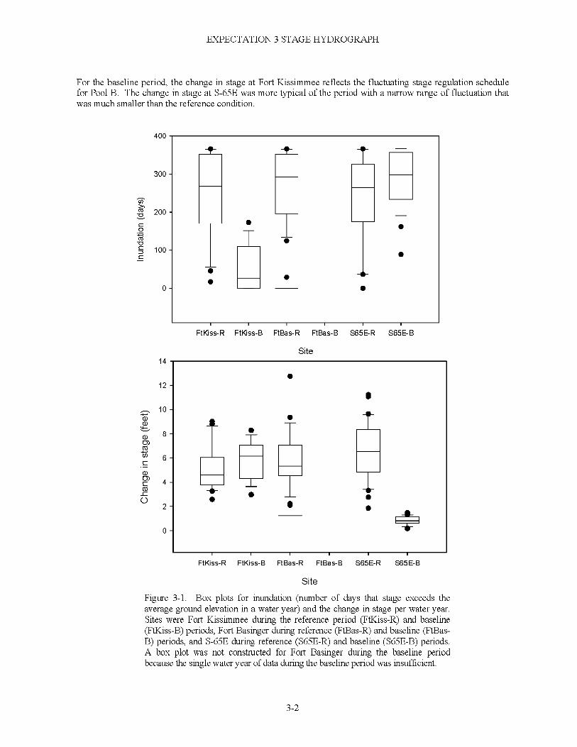
EXPECTATION 3 STAGE HYDROGRAPH

For the baseline period, the change in stage at Fort Kissimmee reflects the fluctuating stage regulation schedule for Pool B. The change in stage at S-65E was more typical of the period with a narrow range of fluctuation that was much smaller than the reference condition.

400

a>a>M—

a>cnro

H— 1toca>cncfi3

_ CO

FtKiss-R FtKiss-B FtBas-R FtBas-B S65E-R S65E-B

S ite

FtKiss-R FtKiss-B FtBas-R FtBas-B S65E-R S65E-B

SiteFigure 3-1. Box plots for inundation (number of days that stage exceeds the average ground elevation in a water year) and the change in stage per water year. Sites were Fort Kissimmee during the reference period (FtKiss-R) and baseline (FtKiss-B) periods, Fort Basinger during reference (FtBas-R) and baseline (FtBas- B) periods, and S-65E during reference (S65E-R) and baseline (S65E-B) periods. A box plot was not constructed for Fort Basinger during the baseline period because the single water year of data during the baseline period was insufficient.

3-2

EXPECTATION 3 STAGE HYDROGRAPH

Reference Conditions

Reference conditions were based on mean daily stage at Fort Kissimmee (Water Year 1943 - 1962), Fort Basinger (Water Year 1933-1959), and S-65E (Water Year 1931-1962).

During the reference period, boxplots for the inundation metric overlapped broadly for Fort Kissimmee, Fort Basinger, and S-65E (Figure 3-1). This overlap suggested that a threshold could be established for any station. For inundation, the 25* percentile was at least 180 d, so a reasonable expectation would be for inundation to be 180 d in most years.

Boxplots for the change in stage metric for the reference period also broadly overlapped, which suggested that a threshold could be established for a desirable minimum fluctuation in stage for most years. The 25th percentile for change in stage during the reference period was 3.75 feet, so that a fluctuation in stage of 3.75 feet might be expected in most years.

Adjustments for External Constraints

Achievement of this expectation depends on completion of the restoration project and the implementation of the headwaters revitalization stage regulation schedule for S-65. It is also highly dependent on rainfall conditions, and it may be necessary to develop a relationship between rainfall and stage using pre-channelization data to modify the expected duration of inundation and the range of stage fluctuation described in this expectation.

Mechanism for Achieving Expectation

Restoration of the physical form of the river through backfilling C-38 and carving new river segments will redirect flows through the Kissimmee River and lead to overflow onto the floodplain. A new regulation schedule and operation rules were developed to provide headwater inflows that reflect climatic inputs to the upper basin and a continuous, seasonally variable flow regime in the restored Kissimmee River. Regulation schedules and operation rules at S-65C and S-65D will be modified to reestablish historic stage-discharge relationships. Slow drainage of water off the floodplain (stage recession rates) also will facilitate reestablishment of floodplain inundation characteristics.

Means of Evaluation

Both the change in water level per water year and inundation are independent of the location so that they can be evaluated at any river channel stage monitoring station along the river. The inundation metric does require that the average ground level at the station be estimated. This expectation will be evaluated for Phase I using data collected at PC33. When Phase II/III is completed, it can be evaluated at Fort Basinger. Evaluation will consist of comparing measured values to the thresholds established in the expectation. If the thresholds are exceeded, the expectation will be achieved.

Time Course

Pre-channelization stage characteristics should be reestablished following the implementation of interim regulation schedules at S-65 and S-65C, backfilling of C-38, and recarving of new river sections. Interim regulation schedules at S-65 and S-65C were implemented in January 2001, and provide for partial reestablishment of historic flows and floodplain hydroperiods. Implementation of the new headwater regulation schedule should begin in late 2010.

Literature Cited

Anderson, D. H., and J. R. Chamberlain. 2005. Impacts of channelization on the hydrology of the Kissimmee River, Florida. Chapter 2 in S. G. Bousquin, D. H. Anderson, G. E. Williams, and D. J. Colangelo, editors. Establishing a baseline: pre-restoration studies of the channelized Kissimmee River. South Florida Water Management District, West Palm Beach, Florida, USA. Technical Publication ERA #432.

3-3

EXPECTATION 3 STAGE HYDROGRAPH

Obeysekera, J., and K. Loftin. 1990. Hydrology of the Kissimmee River Basin - influence of man-made and natural changes. Pages 211-222 in M. K. Loftin, L. A. Toth, and J. T. B. Obeysekera, editors. Proceedings of the Kissimmee River Restoration Symposium. South Florida Water Management District, West Palm Beach, Florida, USA.

3-4

EXPECTATION 4

STAGE RECESSION RATES

Expectation

An annual prolonged recession event will be reestablished with an average duration >173 days and with peak stages in the wet season receding to a low stage in the dry season at a rate that will not exceed 1.0 ft (30 cm) per 30 days.

Author

Joanne Chamberlain, South Florida Water Management District (Current affiliation: BEM Systems Inc.)

April 1, 1999; revised November 2002

Relevant Endpoints

Restoration - Physical Integrity - HydrologyRestoration - Physical Integrity - DisturbanceRestoration - System Functional Integrity - Habitat QualityRestoration - System Functional Integrity - River/Floodplain Interactions

Metrics

Thiity-day stage recession rate Duration of recession events

Baseline Conditions

Baseline conditions were derived from daily average headwater stage at S-65C and S-65D from 1971 to 1998. During the baseline period, stages in Pools C and D were a function of operational schedules for water control structures S-65C and S-65D. Stage fluctuations typically did not vary more than 0.5 ft (15 cm) from control elevations (Figure 4-1). Due to the lack of fluctuation of water levels, there were no significant stage recession events during the baseline period.

Reference Conditions

Reference conditions were derived from daily stage data at Fort Kissimmee (Figure 4-2) and Fort Basinger(Figure 4-3) from 1942 to 1959. Based on these data, peak stages typically occurred in September or October andslowly receded until May or June. Slow stage recession rates provided connectivity between the river and floodplain, which contributed to habitat diversity and functionality, and allowed for the transfer of food resources.

4-1

EXPECTATION 4 STAGE RECESSION RATES

S urface W a te r E levations in P ools C and D

^ 30.00Q>2 28.00 </)

26. CO

24.00

22.00

20. CO

Pool D / S 6 5 D

T - < N C O ^ i r ) O D ^ - ( O C D O T - ( N c o ^ r m a D h - c o c x i O r - < N f o ^ r m a D h - c o( - . h . h - . r - _ h _ r - _ r - - f - - h - - c o c o c o c o c o c o c o c o c o c o c n c r i c r i C D c r > c n c D c r i c n i0 0 ) 0) 0) 0 0 ) 0 0 ) 0) 0) 0 0 0 ) 0) 0 0 ) 0) 0 0 ) 01 0 ) 0 0 0 ) 0) 0) 0) 0)

CO CD CD CO CD CO CD CD CD CD CO CD CD CO CD CD CD tO CD tO CO CO CD CD CO CO tO CD

Figure 4-1. Daily surface water levels atS-65C and S-65D along C-38.

4-2

EXPECTATION 4 STAGE RECESSION RATES

Figure 4 -3. Historic daily surface water levels at Fort Basinger.

Thirty-day recession rates were calculated by the difference in maximum and minimum stages for each recession event divided by the total number of days water levels receded, and multiplied by 30 days (Tables 4-1 and 4-2). Small increases in stage were ignored during prolonged recession events. However, if stage increased >1.5 ft (45 cm), the recession event ended and another event began.

The duration of recession events at Fort Kissimmee (Table 4-1) ranged from 66 to 359 days and averaged 218 days. Stage recession rates ranged from 0.26 to 1.39 ft (8 to 42 cm) per 30 days. Only 1 of the 17 recession events exceeded 1.0 ft (30 cm) per 30 days. In April 1951, a dry season rainfall event caused stages to rise briefly before receding to a seasonal low in June. This recession event lasted 66 days, with water levels receding at a rate of 1.39 ft (42 cm) per 30 days.

The duration of recession events at Fort Basinger (Table 4-2) ranged from 16 to 355 days and averaged 173 days. Stages receded at a rate that ranged from 0.27 to 1.93 ft (8 to 59 cm) per 30 days. Rates of 7 of the 22 recession

events exceeded 1.0 ft (30 cm) per 30 days and were associated with unusual weather conditions. Three events (April 1944, April 1951 and October 1957) resulted from aberrant diy season rainfall, which caused stages to rise briefly before receding to a seasonal low in June. During the recession event of 1948-1949, stage decreased by 8.9 ft (271 cm) and followed two extremely wet years that were due to hurricanes in the Kissimmee valley. In 1955-1956, two of three recession events had short dur ations (<20 days) and occurred early in the wet season prior to the normal seasonal stage recession period from September to May. The October 1956 to February 1957 event lasted 121 days and occurred during a severe drought, which was followed by rainfall that caused stages to increase until October 1957.

Adjustments for External Constraints

Aberrant weather conditions (e.g., El Nino, winter fronts) may cause multiple recession events within a year' and result in shorter average durations and recession rates that may exceed 1.0 ft (30 cm) per 30 days.

4-3

EXPECTATION 4 STAGE RECESSION RATES

Table 4-1. Historic stage recession rates at Fort Kissimmee. Events exceeding the 1.00 ft/30 d recession rate are in bold.

Year Start Date„ , Start End End Date Stage (ft) stage (ft)

Change in Stage (ft)

Duration(days)

Rate(ft/day)

Rate(ft/30days)

# of Events per Year

1942-43 3-Sep-42 12-May-43 45.7 40.9 4.8 251 0.02 0.58 1

1943 44 11-Oct-4 3 5-Jun-44 45.2 40.9 4.3 238 0.02 0.55 11944 45 26-Oct-44 20-Jun-45 45.5 41.1 4.4 237 0.02 0.55 1

1945-46 18-Sep-45 13-May-46 50.1 43.3 6.8 237 0.03 0.87 1

1946 47 22-Sep-46 12-Feb-47 46.3 43.9 2.4 143 0.02 0.5 11947-48 23-Sep-47 1-Jul-48 49.8 43.9 6 282 0.02 0.63 1

1948-49 4-Oct-48 31-May-49 49.7 41.9 7.9 239 0.03 0.99 11949-50 1-Oct-4 9 28-Aug-50 48.1 40.7 7.4 331 0.02 0.67 1

1950-51 31-0ct-50 30-Mar-51 44.4 42.8 1.5 150 0.01 0.3122-Apr-51 2 7-Jun-51 44.8 41.8 3.1 66 0.05 1.39

1951-52 20-Nov-51 30-Jun-52 45.2 43.3 2 223 0.01 0.26 1

1952-53 23-Oct-52 3-Jun-5 3 47 43.6 3.4 223 0.02 0.46 1

1953-54 No Data — — — — — — — —

1954-55 1-Oct-5 4 19-Jun-55 45.4 40.6 4.9 261 0.02 0.56 1

1955-56 13-Sep-55 27-May-56 44.1 38.6 5.5 257 0.02 0.64 1

1956-57 17-Oct-56 20-Feb-57 47.3 43.5 3.8 126 0.03 0.9 11957-58 5-Oct-57 22-Dec-57 46.5 44.8 1.7 78 0.02 0.66 1

1958-59 28-Jan-58 22-Jan-59 46.4 42.1 4.4 359 0.01 0.36 1

Table 4-2. Historic stage recession rates at Fort Basinger. Events exceeding the 1.00 ft/30 d recession rate are in bold.

Year Start Date End DateStart

Stage (ft)End Stage Change in Duration

(ft) Stage (ft) (days)Rate

(ft/day)Rate

(ft/30days)# of Events

per Year

1942-43 3-Oct-42 21-May-43 31.4 26 5.4 230 0.02 0.71 15-Oct-43 29-Mar-44 32.2 27.4 4.8 176 0.03 0.82 2

1943-4419-Apr-44 6-Jun-44 29.2 26.2 3.1 48 0.06 1.93

1944-45 5-Nov-44 21-Jun-45 30.7 25.8 4.9 228 0.02 0.64 11945-46 22-Sep-45 14-May-46 34.6 28 6.6 234 0.03 0.85 11946-47 17-Sep-46 11-Feb-47 31.2 28.8 2.3 147 0.02 0.48 11947-48 24-Sep-47 3-Jul-48 34.9 29.2 5.7 283 0.02 0.6 11948-49 6-Oct-48 1-Jun-49 35.5 26.6 8.9 238 0.04 1.12 11949-50 5-Oct-49 4-Jun-50 33.2 27 6.2 242 0.03 0.77 1

26 0ct-50 6-Apr-51 31.6 27.5 4.1 162 0.03 0.76 21950-51

24-Apr-51 27-Jun-51 30.7 27.8 2.9 64 0.05 1.371951-52 3-Oct-51 25-Mar-52 32.8 29.2 3.6 174 0.02 0.62 11952-53 28-Oct-52 4-Jun-53 32.7 29.4 3.3 219 0.02 0.46 11953-54 13-Oct-53 25-May-54 36.1 29.5 6.6 224 0.03 0.88 11954-55 20-Jun-54 10-Jun-55 32 25.9 6.1 355 0.02 0.52 1

4-Jul-55 20-Jul-55 29.5 27.4 2.1 16 0.13 . . . 31955-56 ll-A u g -5 5 30-Aug-55 29.4 27.4 2 19 0.11 . . .

19-Sep-55 29-May-56 28.9 24 4.9 253 0.02 0.581956-57 21-Oct-56 19-Feb-57 33.2 28.1 5.2 121 0.04 1.28 1

7-Oct-57 22-Dec-57 32.5 29.6 2.9 76 0.04 1.13 21957-58

3-Feb-58 20-Jun-58 31.6 30.4 1.2 137 0.01 0.271958-59 20-Jul-58 25-Dec-58 30.8 26.8 4 158 0.03 0.76 1

4-4

EXPECTATION 4 ST AGE RECESSION RATES

Mechanism for Achieving Expectation

Reestablishment of slow stage recession rates will be achieved by restoring the physical form of the Kissimmee River, implementing new regulation schedules, and reestablishing wetland vegetation on the floodplain. Backfilling C-38 and carving new river segments will direct flows through the river and floodplain. A new headwater regulation schedule and operation rules will provide continuous inflows to the Kissimmee River. Regulation schedules and operation rules based on historic stage-discharge relationships at downstream structures (S-65C and S-65D) and the limited conveyance of the restored river and floodplain will control recession rates in the restored system.

2 0 2 4 M i le s

Figure 4-4. Locations of stations that will be used to evaluate stage recession rates along the restored river for Phase I of the restoration project.

4-5

EXPECTATION 4 STAGE RECESSION RATES

Means of Evaluation

Recession rates will be calculated annually using daily stage data collected at PC33, PC43, and PC54 in Pool C (Figure 4-4). A recession event will begin with the peak wet season stage and continue to a dry season low. Small increases in stage will be ignored. However, if the stage increase exceeds 1.5 ft (45 cm), the recession event will end and another event will begin. Thirty-day recession rates will be calculated by the difference in maximum and minimum stages for each recession event divided by the total number of days water levels receded, and multiplied by 30 days. The expectation will be achieved if the average duration of recession events is >173 days and recession rates are <1.0 ft (30 cm) per 30 days.

Time Course

Natural stage recession rates will be reestablished following implementation of the new headwater regulation schedule, which is scheduled for 2010. Interim regulation schedules at S-65 and S-65C were implemented in June 2001 and provide for partial reestablishment of historic inflows, stage fluctuations, and stage recession rates. Evaluation of the average duration and rate of recession events will require a minimum of ten years of data. This

data set should include the average annual historic stage fluctuations [~4 to 6 ft (122 to 183 cm)].

4-6

EXPECTATION 5

RIVER CHANNEL VELOCITIES

Expectation

Mean velocities within the main river channel will range from 0.8 to 1.8 ft/s (0.2 to 0.6 m/s) a minimum of 85% of the year.

Author

Joanne Chamberlain, South Florida Water Management District (Current affiliation: BEM Systems Inc.)

June 1,1999; revised November 16, 2002

Relevant Endpoints

Restoration - Physical Integrity - HydrologyRestoration - Physical Integrity - Hydrogeomoiphic ProcessesRestoration - System Functional Integrity - Habitat Quality

Metrics

Frequency of mean channel velocity

Baseline Conditions

Baseline conditions were derived from daily discharge at site PC33 on Micco Bluff Run, a remnant river channel in Pool C. Data from this site is representative of baseline conditions (November 1997-May 1999) within remnant river channels that will be affected by the first phase of restoration.

Daily discharge at PC33 ranged from 0 to 1170 tf/s (33 m3/s), but flows greater than 100 tf/s (2.8 mVs) occurred only 5% of the time. Mean channel velocities were calculated by dividing discharge by the cross sectional area of the river channel and ranged from 0.0 to 1.61 ft/s (0.49 m/s). However, because remnant river channels rarely conveyed discharge, mean channel velocities were less than 0.8 ft/s (0.2 m/s) 99% of the baseline period.

Reference Conditions

Reference conditions were derived from the U. S. Geological Survey (USGS) historic stream gauging data at the Kissimmee River below Lake Kissimmee (USGS site 2269000) and at the Kissimmee River near Comwell/Bassinger (USGS site 2272500). A total of 342 measurements were collected between 1931 and 1959 (309 below Lake Kissimmee and 33 near Comwell/Bassinger). Of these measurements, 179 were rated fair to excellent by the USGS and were used to derive mean velocities in the main river channel, which ranged between 0.8 to 1.8 ft/s (0.2 to 0.6 m/s) during 93% of these sampling events (Figure 5-1). Main channel discharges associated

5-1

EXPECTATION 5 RIVER CHANNEL VELOCITIES

with velocities between 0.8 to 1.8 ft/s (0.2 to 0.6 m/s) ranged from approximately 100 to 2100 ftVs (3 to 59 m3/s), with flows exceeding 500 ftVs (15 m3/s) during 88% of the sampling events.

100.0%

w 90.0%

0 80.0%

1 70.0%

$ 60.0%

O 50.0%

O 40.0%

g 30.0%

£ 20.0%

10.0%

0.0%

Figure 5-1. Frequency distribution of mean channel velocities near Fort Bassinger (n=24) and downstream of Lake Kissimmee (n=155). Data were collected during stream gauging events and are not from continuous monitoring.

Adjustments for External Constraints

None

Mechanism for Achieving Expectation

Backfilling C-38 and carving new river segments to connect remnants of the historic river channel will restore the physical form of the Kissimmee River, which will then convey flows.

Implementation of a new headwater regulation schedule and operation rules will provide continuous headwater inflows that reflect climatic inputs to the upper basin and a more natural, seasonally variable flow regime. Water regulation schedules and operation rules for downstream control structures (S-65C and S-65D) will be modified to maintain historic surface water gradients and associated velocities along the restored river. Downstream control of water levels is needed to ensure that unnaturally high and potentially erosive velocities do not occur within the river channel. New regulation schedules and operation rules for S-65C and S-65D will be based on estimated historic stage-discharge relationships at these locations. S-65C is the downstream control for Phase I of restoration. S-65D will serve as the downstream control for the entire restoration project and will be established at the completion of Phase II/III.

Reference Period (1931 - 1959)

93%

< 0.8 0 . 8 - 1.8 > 1.8

Mean Channel Velocity (ft/s)

5-2

EXPECTATION 5 RIVER CHANNEL VELOCITIES

Means of Evaluation

The historic range and frequency of mean velocities within the main river channel will be compared to post-restoration conditions. Daily stage and discharge data will be used to calculate mean channel velocities in the restored river by dividing discharge by cross sectional area. Bathymetric surveys of channel cross sectional area will be collected at least twice a year to monitor changes to hydraulic geometry.

Post-restoration evaluations will begin at the completion of Phase I and Phase II/III construction. Mean channel velocities at PC33 will be used to evaluate post-restoration velocities for Phase I. Data from a new discharge/velocity station established within a section of river restored during Phase II/III will be compared to historic conditions after the completion of Phase II/III backfilling. A minimum of three years of data will be used for evaluation of each phase of the project and should include the historic distribution of flows. The expectation will be achieved if a minimum of 85% (annually) of mean daily velocities within the main river channel range between 0.8 and 1.8 ft/s (0.2 to 0.6 m/s) for a minimum of three years after each phase of restoration.

Time Course

Reestablishment of the frequency of historic mean channel velocities will occur following backfilling of C-38, recarving of new river sections, and implementation of new regulation schedules. Implementation of the new headwater regulation schedule cannot begin until all real estate interests have been acquired along Lakes Kissimmee, Hatchineha and Cypress, which is tentatively scheduled for 2010. However, interim regulation schedules at S-65 and S-65C were implemented in January 2001 and provide for partial reestablishment of historic headwater inflows.

5-3

EXPECTATION 6

RIVER CHANNEL BED DEPOSITS

Expectation

In remnant river channels, mean thickness of substrate-overlying river bed deposits will decrease by >65%, percent of samples without substrate-overlying river bed deposits will increase by >165%, and the thickness of substrate-overlying river bed deposits at the thalweg will decrease by >70%

Author

David H. Anderson, South Florida Water Management District Pat Davis, South Florida Water Management DistrictDon Frei, South Florida Water Management District (Current affiliation: National Marine Fisheries Service)

June 29,1999; revised June 26, 2002

Relevant Endpoints

Physical Integrity - River Channel Substrate Characteristics Physical Integrity - Hydrogeomorphic Processes System Functional Integrity - Habitat Quality System Functional Integrity - Habitat Diversity

Metrics

Mean thickness of substrate-overlying deposits Percent of samples without substrate-overlying deposits Thickness of substrate-overlying deposits at the thalweg

Baseline Condition

Organic deposits and, to a lesser extent, mail deposits have accumulated on the natural channel bed in all remnant river channels since channelization (Toth 1991; 1993). Much of this organic matter is derived from floating aquatic plants and rooted macrophytes, which in the absence of flow have expanded their coverage in mid-channel and littoral areas, respectively. As these plants die, they are a source of organic deposition. The thickness and distribution of these deposits were quantified by taking core samples on 86 transects across remnant river channels in the Impact area (Pools B and C) and 21 transects in the Control area (Pool A) during 1997-1999 (Anderson et al. 2005). Deposits on the pre-channelization channel bed substrate were quantified for each transect with three metrics: (1) mean thickness of substrate-overlying deposits, (2) percent of samples without substrate-overlying deposits, (3) and the thickness of substrate-overlying deposits at the thalweg. Mean thickness of substrate-overlying deposits estimates the amount of deposition on a transect by averaging the thickness of substrate-overlying deposits for all cores from that transect. Percent of samples without substrate-overlying deposits is the percent of samples on a transect without such deposits above the substrate layer. Thalweg

6-1

EXPECTATION 6 RIVER CHANNEL BED DEPOSITS

deposition thickness is the thickness of the substrate-overlying deposits at the deepest part of the channel and estimates the amount of deposition above the substrate layer in the portion of the channel cross-section that should have the least deposition because it experiences the highest water velocities and thus the greatest tractive forces. Each of these metrics was estimated for each transect, and the values were averaged across transects to obtain a mean and a standard error for transects in the Impact and Control areas. Mean + standard error thickness of the substrate-overlying deposits was 14 ± 0.7 cm in the Impact area and 22 ± 1.9 cm in the Control area. Percent of samples without substrate-overlying deposits was 3 + 0.65% in the Impact area and 1 + 0.4% in the Control. The thickness of substrate-overlying deposits at the thalweg averaged 21 + 2.2 cm in the Impact area and 38 + 5.1 cm in the Control area.

Reference Condition

Prior to channelization, the river bed substrate was composed primarily of deposits of fine and medium-grained sands intermixed with shells, silt, and clay that were laid down during the late Miocene/Pleistocene epochs (Wame et al. 2000). In baseline core samples from Control and Impact areas, the substrate beneath the accumulated organic/marls deposits was primarily sand (Anderson et al. 2005).

Because pre-channelization data were not available, data collected during the Kissimmee River Demonstration Project (1985-1988) (Toth 1991; 1993) were used as the reference condition for expected changes in substrate- overlying deposits. During the Demonstration Project, weirs were used to divert up to 60% of the flow through the C-38 canal to each of three remnant river channels (Rl, R2, and R3) in Pool B (Toth 1993). Between April 1985 and December 1988, each remnant channel had flow >26 m3/s, which approaches bankfull discharge, for 233-307 days (Toth 1991). River channel sediments were characterized by collecting core samples using similar methods to those used for the baseline study on 24 transects across these remnant river channels. Transects were sampled one time before reestablishing flow, and up to six times after flow was reestablished, which allowed the tracking of changes in the three metrics used for the baseline study. Mean thickness of the substrate-overlying deposits declined from 15 cm to 5 cm, a 67% reduction (Figure 6-1). Percent of samples without substrate- overlying deposits increased from an average of 21% to 56%, an increase of 167%. The thickness of substrate- overlying deposits at the thalweg decreased by 70% from an average of 30 cm to 9 cm. These reference values are likely to be conservative estimates of the condition of the river bed substrate before channelization because these metrics continued to change (Figure 6-1) and because the magnitude and duration of flow was less than what was observed prior to channelization. Achieving these values within three years of reestablishing flow indicates the reestablishment of processes that determine river bed substrate characteristics. These processes will likely continue until the channel adjusts to the restored flow conditions.

Mechanism for Achieving Expectation

Backfilling of the C-38 canal and carving new river channels to connect the remnant channels should restore flow to the river channel. Reestablishing the pre-channelization flow regime to reconnected river channels should flush the accumulated layer of organic and marl deposits or bury it beneath sand that is transported by flow. Maintaining continuous flow will reduce the loading of organic matter deposited on the channel substrate by reducing the mid-channel cover of floating aquatic vegetation, and restricting rooted macrophytes, such as Nuphar lutea and Polygonum densiflorum, to the channel littoral zone. Reducing the area of rooted macrophytes bed should also reduce the capability of the river channel to retain organic matter, because the roots of these plants can help trap organic particles.

Adjustments for External Constraints

None

Means of Evaluation

Post-construction core sampling will be conducted at the same permanent transects in the Impact and Control areas established for the baseline study. Interim evaluation of the three metrics will be conducted annually by sampling 24 randomly selected transects from the Impact area during the dry season. When all expectation

6-2

EXPECTATION 6 RIVER CHANNEL BED DEPOSITS

metrics have been achieved for the interim transects, all transects in the Control and Impact areas will be sampled during the following dry season. The expectation will be evaluated by comparing the observed values to those stated in the expectation. The expectation will be considered achieved if mean thickness of the substrate- overlying deposits decreases by >65%, if the percent of samples without substrate-overlying deposits increases by >165%, and if the thickness of substrate-overlying deposits at the thalweg decreases by >70%.

Date

Figure 6-1. Mean values (^standard error) for (A) mean thickness of substrate-overlying deposits, (B) percent of samples without substrate-overlying deposits, and (C) the thickness of substrate- overlying deposits at the thalweg during the Kissimmee River Demonstration Project. The first sample date is prior to the weirs being installed and combines data from November 1984 for R3, March 1985 for R2, and July 1985 for R1.

6-3

EXPECTATION 6 RIVER CHANNEL BED DEPOSITS

Time Course

Based on results of the Pool B Demonstration Project, flushing of the depositional layer overlying the substrate,and changes in the river bed should occur within three years of reestablishing the pre-channelization flow regime.

Literature Cited

Anderson, D. H., D. Frei, and W. P. Davis. 2005. River channel geomorphology of the channelized Kissimmee River. Chapter 3 in S. G. Bousquin, D. H. Anderson, G. E. Williams, and D. J. Colangelo, editors. Establishing a baseline: pre-restoration studies of the Kissimmee River. South Florida Water Management District, West Palm Beach, Florida, USA. Technical Publication ERA #432.

Toth, L. A. 1991. Environmental responses to the Kissimmee River demonstration project. Technical Publication 91-02. South Florida Water Management District, West Palm Beach, Florida, USA.

Toth, L. A. 1993. The ecological basis for the Kissimmee River restoration plan. Florida Scientist 56:25-51.

Wame, A. G., L. A. Toth, and W. A. White. 2000. Drainage-basin-scale geomorphic analysis to determine reference conditions for ecological restoration - Kissimmee River, Florida. Geological Society of America Bulletin 112:884-899.

6-4

EXPECTATION 7

SAND DEPOSITION AND POINT BAR FORMATION INSIDE RIVER CHANNEL BENDS

Expectation

Point bars will form on the inside bends of river channel meanders with an arc angle >70°.

Author

Don Frei, South Florida Water Management District (Current affiliation. National Marine Fisheries Sendee)Pat Davis, South Florida Water Management District David H. Anderson, South Florida Water Management District

June 29,1999; revised April 3, 2001

Relevant Endpoints

Ecological Integrity/Restoration/Physical Integrity - River Channel Substrate Characteristics Ecological Integrity/Restoration/Physical Integrity - Hydrogeomorphic Processes Ecological Integrity/Restoration /System Functional Integrity - Habitat Quality Ecological Integrity/Restoration /System Functional Integrity - Habitat Diversity

Metrics

Number of meanders with point bars

Baseline Conditions

Aerial photographs taken since channelization indicate that active point bars (i.e., sand deposition found on the inside bend of meanders) are not visible in remnant river channels (Anderson et al. 2005). Point bare that were present in the pre-channelized system have been colonized by vegetation, and elimination of flow has precluded development of new bars. Cross sectional profiles show a remnant sloping riverbed along inner portions of meanders remains, but submerged portions of these relic point bars are covered with organic deposits or aquatic vegetation.

Reference Conditions

Point bars were likely an important habitat feature in the historic Kissimmee River. Point bars provided topographic diversity and a range of flow velocities useful to many species (Bain et al. 1988, Lobb and Orth 1991, Sheldon and Meffe 1995), and likely provided spawning habitat for pit nesters (e.g., centrarchids) (L. Glenn, personal communication), refuge and foraging habitat for small fish, and habitat for shore birds and foraging

7-1

EXPECTATION 7 SAND DEPOSITION AND POINT BAR FORMATION

wading birds. Point bars are typical of rivers with sinuous, low-gradient, meandering channels, sandy substrates, and well-developed floodplains in broad drainage basins (Leopold 1994, Rosgen 1994, 1996).

We quantified the occurrence of point bars using historical aerial photographs during extreme low water levels (38.64 NGVD at Fort Kissimmee) in June 1956. Point bars occurred on the inside of 329 of 330 river meanders with an arc angle >70°. We used an arc angle of 70° (Rosgen 1996) to distinguish meander bends from minor curvature of the channel. Largest point bars occurred on curves downstream of long, straight river runs.

Point bars formed on inside curves of meanders after flow was partially restored to remnant river channels in Pool B (Toth 1993). After the Test Fill Plug was constructed in 1994 (Koebel et al. 1999), point bars in the adjacent remnant river channel increased in area and height, particularly after high flows in winter 1998.

Mechanism for Achieving Expectation

Point bar formation is a result of sediment transport and deposition and has a well-documented relationship to river suspended sediment size and flow velocities (Knighton 1998). Restoration of point bars will be dependent on the discharge volume and duration of flow. Reestablishment of historical flow regimes (e.g., bankfull discharge of 40-50 m3/s) is expected to reestablish active point bar formation on inside curves of meanders in remnant river channels.

Adjustments for External Constraints

None

Means of Evaluation

Point bar formation will be monitored annually for five years after reestablishment of flow through the river channel. The formation or reappearance of point bars will be tracked and georeferenced with GPS along 80 meanders with an arc angle >70° within Pool C and lower Pool B. This area will be affected by restored flow from the first phase of the restoration project.

Time Course

Based on sediment transport and deposition in Pool B during the Kissimmee River Demonstration Project of 1985-1988 and after the Test Fill Plug construction in 1994, point bar formation will occur following bankfull discharge events. Reestablishment of pre-channelization point bar distribution will occur within three to five years, depending on the magnitude and duration of bankfull discharge.

Literature Cited

Anderson, D. H., D. Frei, and W. P. Davis. 2005. River channel geomorphology of the channelized Kissimmee River. Chapter 3 in S. G. Bousquin, D. H. Anderson, G. E. Williams, and D. J. Colangelo, editors. Establishing a baseline: pre-restoration studies of the Kissimmee River. South Florida Water Management District, West Palm Beach, Florida, USA. Technical Publication ERA #432.

Bain, M. B., J. T. Finn, and H. E. Brooke. 1988. Streamflow regulation and fish community structure. Ecology 69:382-392.

Knighton, D. 1998. Fluvial forms and processes. Arnold, London, UK.

Koebel, J. W., B. L. Jones, and D. A. Arrington. 1999. Restoration of the Kissimmee River, Florida: water quality impacts from canal backfilling. Environmental Monitoring and Assessment 57:85-107.

Leopold, L. B. 1994. A view of the river. Harvard University Press, Cambridge, Massachusetts, USA.

Lobb, M. D., and D. J. Orth. 1991. Habitat use by an assemblage of fish in a large warmwater stream. Transactions of the American Fisheries Society 120:65-78.

Rosgen, D. L. 1994. A classification of natural rivers. Catena 22:169-199.

7-2

EXPECTATION 7 SAND DEPOSITION AND POINT BAR FORMATION

Rosgen, D. L. 1996. Applied river morphology. Wildland Hydrology Books Inc., Pagosa Springs, Colorado, USA.

Sheldon, A. L., and G. F. Meffe. 1995. Path analysis of collective properties and habitat relationships of fish assemblages in coastal plain streams. Canadian Journal of Fisheries and Aquatic Sciences 52:23-33.

Toth, L. A. 1993. The ecological basis of the Kissimmee River Restoration Plan. Florida Scientist 56:25-51.

7-3

EXPECTATION 8

DISSOLVED OXYGEN CONCENTRATIONS IN THE RIVER CHANNEL

Expectation

Mean daytime concentration of dissolved oxygen in the Kissimmee River channel at 0.5-1.0 m depth will increase from <1-2 mg/L to 3-6 mg/L during the wet season (June-November) and from 2-4 mg/L to 5-7 mg/L during the dry season (December-May). Mean daily concentrations will be greater than 2 mg/L more than 90% of the time. Dissolved oxygen concentrations within 1 m of the channel bottom will exceed 1 mg/L more than 50% of the time.

Author

David J. Colangelo , South Florida Water Management District Brad Jones, South Florida Water Management District

June 10, 1999; revised March 4, 2002

Relevant Endpoints

Restoration - Chemical Integrity - Surface Water Quality Restoration - Chemical Integrity - Dissolved Oxygen Dynamics Restoration - System Functional Integrity - Habitat Quality

Metrics

Mean wet season daytime concentration of dissolved oxygen at 0.5 m Mean diy season daytime concentration of dissolved oxygen at 0.5 m Annual percentage of samples with dissolved oxygen concentrations >2 mg/L Percent of time with dissolved oxygen concentrations near the bottom >1 mg/L

Baseline Condition

Concentrations of dissolved oxygen (DO) in stagnant river runs are frequently below 1 mg/L, even near the water surface at midday. During 1996 through 1999, mean concentrations (0.5 m depth) in monthly sampling in seven river runs in Pools A and C (Table 8-1) ranged from 0.7 to 1.9 mg/L during the wet season and from 2.5 to 3.8mg/L during the dry season (Figure 8-1). Dissolved oxygen exceeded 2 mg/L in <60% of the measurements andexceeded 5 mg/L in <20% of the measurements (Figure 8-2). At two stations (Oxbow 13 and Montsdeoca Run) with continuous (one reading even' 15 minutes at 1.0 m) monitoring, DO concentrations exceeded 2 mg/L for 22% of the baseline period of record (July 1997-June 1999) and exceeded 5 mg/L for 6% of this period (Figure 8-3).

8-1

EXP 8 DISSOLVED OXYGEN

Depth profile data from May-June 1999 in Pool C (D. Colangelo, unpublished data), and from earlier years in Pool B, show DO values typically ranging from 2-3 mg/L at the water surface, and declining to <1 mg/L below a 1.0 m depth during summer months (Rutter et al. 1986, Toth 1991).

Table 8-1. Dissolved oxygen concentrations in the channelized Kissimmee River and other Florida streams (reference sites).

Water Body SFWMD Reference ID County Period of Record

(month/yr) Frequency1 # Samples

Reference SitesFisheating Creek FECSR78 Glades 4/73-2/99 W-M 447Arbuckle Creek ARBKSR98 Highlands 2/88-2/99 BiM 86Lake Marian Creek DLMARNCR Polk 4/82-9/85 M 37Tiger Creek ETIGERCR Polk 4/82-6/85 M 33Josephine Creek JOSNCR17 Highlands 2/88-2/99 M-BiM 85Boggy Creek ABOGG Osceola 8/81-3/99 M 202Catfish Creek ROSALIEC Polk 11/84-9/85 M 11

Kissimmee RiverIce Cream Slough Run (Pool A) KREA 97 Polk 11/96-3/99 M 27Rattlesnake Hammock Run (Pool A) KREA91 Polk 3/96-3/99 M 29Schoolhouse Run (Pool A) KREA 92 Polk 3/96-3/99 M 31Montsdeoca Run (Pool C) KREA 98 Highlands 3/96-3/99 M 14Oxbow 13 (Pool C) KREA 93 Highlands 3/96-3/99 M 29Micco Bluff Run (Pool C) KREA 94 Okeechobee 3/96-3/99 M 28MacArthur Run (Pool C) KREA 95 Highlands 12/97-3/99 M 31*W = Weekly; M = Monthly; BiM = Bi-Monthly

Reference Condition

No DO data were collected before channelization, so the reference condition has been derived from data on seven free-flowing, blackwater, south Florida streams. Multiple metrics were used to describe DO regimes. Mean DO concentrations change seasonally due to differences in water temperature and community metabolism. Anoxic benthic conditions can severely limit available habitat for aerobic organisms, and DO concentrations less than 2 mg/L are considered uninhabitable by many aquatic species. Each stream had at least 11 samples collected over a minimum of one year, and some streams were sampled for more than ten years (Table 8-1). Measurements were taken with a DO probe at 0.5 m depth, at intervals ranging from weekly to bimonthly. Mean DO concentrations ranged from 2.4 to 6.0 mg/L during the wet season and from 3.7 to 7.4 mg/L during the dry season (Figure 8-1). In five of the seven streams, DO was >5 mg/L in more than 50% of the samples. More than 90% of the samples had concentrations greater than 2 mg/L in all streams. All streams had DO concentrations >1 mg/L over 90% of the time (Figure 8-2). Although no water column profile data have been examined for these streams (and in most cases do not exist), it is assumed that oxygen values near the bottom are usually higher when streamflow is present. This was observed during the Pool B Kissimmee River Demonstration Project when weirs across C-38 diverted flow to adjacent remnant river runs. Although oxygen concentrations remained low, more uniform DO profiles were observed during the summer (Rutter et al. 1989).

8-2

EXP 8 DISSOLVED OXYGEN

H BaselineI I Reference

Wet season

Dry season

T— CN CO '=r in r*- COCD O) CT) CT) <y> CT> CT)

< < < < < < <LU LU LU LU LU LU LUcr cr cn QC cr CU

Station

Figure 8-1. Mean (± standard error of the mean) dissolved oxygen (DO) concentrations m free-flowing, blackwater, south Florida streams and remnant runs of the channelized Kissimmee River during the wet (June-Nov ember) and dry (December-May) season. Cross-hatched area represents expected range of DO concentrations in the Kissimmee River after restoration.

These reference streams may not completely represent conditions that existed in the pre-channelized river. Artificial drainage, nonpoint-source runoff and point source effluent may increase oxygen demand in these streams and other factors such as headwater characteristics, flow velocities, and water depth may differ from the pre-channelized Kissimmee River. However, due to similarities in flow, watershed characteristics, and water quality, these streams exemplify oxygen regimes in the former river.

8-3

EXP 8 DISSOLVED OXYGEN

Using these streams as a reference, the mean concentration of DO in the Kissimmee River (center of channel, near water surface, at midday) was estimated to be between 3-6 mg/L during the wet season and between 5-7 mg/L during the dry season.

Dissolved Oxygen (m g/L)

Figure 8-2. Dissolved Oxygen concentrations at 0.5 m depth in south Florida reference streams and remnant runs of the channelized Kissimmee River.

Adjustments for External Constraints

Dissolved oxygen concentrations in the upper reach of the restored segment will continue to reflect oxygen- depleted inputs from C-38.

Mechanism for Achieving Expectation

Restoration of contmuous, variable flow through the historic river channel is expected to flush flocculent organic matter, and increase DO concentrations by reducing biochemical and sediment oxygen demand and by increasing atmospheric aeration. Continuous channel flow should inhibit encroachment by aquatic macrophytes, so the need for herbicide treatments should be reduced, Continuous flow should limit accumulation of organic matter. Higher water levels and more natural hydropatterns will lead to less input of oxygen-depleted groundwater.

8-4

EXP 8 DISSOLVED OXYGEN

Means of Evaluation

Monthly data collection will continue at the seven remnant run stations that were sampled during the baseline period (Table 8-1) (see Time Course section below). This data will be used to evaluate changes in mean daytime wet and dry season DO concentrations. Mean DO values are useful measures of changes in the DO regime because mean values limit the influence of short-term extremes. Aquatic biota inhabiting south Florida streams are tolerant of short-term (10-24 hours) low DO conditions. Other monitoring stations in the canal and remnant runs, including up to eight stations with 24-hour (96 samples/day) automated monitoring, will be used to evaluate if mean daily DO concentrations exceed 2 mg/L 90% of the time. At some of these stations, weekly water quality profiles are collected throughout the water column. Data from these stations will be used to evaluate changes in DO gradient. Pre- and post-restoration data will be compared, and post-restoration data will be compared to the reference data and data from Pool A Increased DO within the Pool C runs will be evaluated by statistical tests, frequency analysis (e.g., Figure 8-2), and time series analysis.

1 0 0

9 0

-_o 8 0oO 7 0<_>CD

ct: 6 0' o“OO 5 0<D

Cl 4 0o£= 3 0CD<_><D 2 0Q_

1 0

□

0 1 2 3 4 5 6 7 8 9 10

______________________________ D isso lved O xygen (m g /L )______________________

Figure 8-3. Percent of period of record (July 1997-June 1999) that Dissolved oxygen (DO) within remnant river channels exceeded x-axis values. Data are based on mean (average of 96 values per day) daily DO concentrations at two remnant river run stations in Pool C (Oxbow 13 and Montsdeoca Run). Dissolved Oxygen readings were taken at a depth of 1.0 m at each station.

To evaluate how DO responds to diversion of flows to the remnant runs, four other sample stations were established during April 1999 in remnant river runs near the canal C-38 backfilling. At each of these stations, DO profiles are sampled weekly with a water quality probe. Monitoring stations will be moved or added as the construction activity moves upstream. This sampling network will include three automated stations for 24-hour monitoring in the river runs. Automated stations can monitor DO during the lowest portion of the diel cycle and during periods of severe hypoxia, while daytime monitoring will gather measurements from a wider network of stations and allow comparisons with data from reference streams. All sampling will continue for three to five years after construction is complete to ensure that changes in DO regimes are not transitory.

Time Course

All metrics for DO concentrations in the river channel are expected to be met within two years after all phases of construction are complete and continuous flow is restored to the river channel. An interim water level operation plan was implemented in January 2001 and will at least partially reestablish hydrological characteristics required

8-5

EXP 8 DISSOLVED OXYGEN

for restoration. Daytime concentrations of DO will begin to improve when construction has recreated enough of the historic river channel to allow continuous flow, reaeration, and restored channel characteristics to significantly affect the oxygen balance. Because little improvement in DO was observed during the Pool B Demonstration Project (Rutter et al. 1989), it is likely that flow must be restored to more than one remnant river segment to significantly affect DO concentrations in the restored reach of the river. Therefore, improvement in the diel oxygen cycle may not be observed until backfilling extends upstream of Micco Bluff Run, and flow is restored to the reconnected Micco Bluff and MacArthur Runs. Improvement in DO conditions will be most evident during the wet season because wet season baseline DO concentrations are very low.

During backfilling, DO may be affected by mobilization of organic sediments and decayed vegetation in the channel and floodplain. However, these events should not have a persistent ecological impact.

Literature Cited

Rutter, R. P., D. E. Sessions, G. M. Sloane, and D. A. Winkler. 1986. Kissimmee River Restoration Project: pre­construction monitoring. Florida Department of Environmental Regulation, South Florida District, Punta Gorda, Florida , USA

Rutter, R. P., D. E. Sessions, and D. A. Winkler. 1989. Kissimmee River Restoration Project: post-construction monitoring. Florida Department of Environmental Regulation, South Florida District, Punta Gorda, Florida, USA.

Toth, L. A. 1991. Environmental responses to the Kissimmee River Demonstration Project. Technical Publication 91-02. South Florida Water Management District, West Palm Beach, Florida, USA.

8-6

EXPECTATION 9

TURBIDITY AND SUSPENDED SOLIDS CONCENTRATIONS IN THE RIVERCHANNEL

Expectation

Mean turbidity in the restored river channel will not differ significantly from mean turbidity in similar south Florida streams (3.9NTU), and the median total suspended solids concentration will not exceed 3 mg/L.

Author

Brad Jones, South Florida Water Management District

June 8,1999; revised June 18, 2003

Relevant Endpoints

Impact Assessment - Water Quality

Metrics

Mean turbidityMedian total suspended solids

Baseline Condition

Turbidity and total suspended solids (TSS) were very low in all remnant river runs sampled during 1996-1999 (Table 9-1). Mean turbidity ranged from 1.3 to 3.5 NTU. Total suspended solids concentrations were <25 mg/L, and were usually lower than the detection limit (i.e., <3 mg/L). Slightly higher turbidity values were measured in summer, and appeal' to reflect greater densities of phytoplankton, as indicated by chlorophyll a concentrations (Figures 9-1 and 9-2).

Reference Condition

No turbidity or TSS data were collected before the river was channelized, so the reference condition was derived from general knowledge of pre-channelized conditions and data on other south Florida streams. Turbidity in the former river is assumed to have been very low due to: (1) the river’s location in a watershed with nearly flat topography, sandy soils, and low-intensity land use; (2) headwater inflow from Lake Kissimmee; (3) low channel velocities; and (4) filtering effects of marsh and littoral vegetation. Turbidity caused by eroded particles from the watershed should have been negligible, and any turbidity present would have been due to plankton, suspended detritus, or sediment erosion during extreme flows. In a flowing blackwater river surrounded by dense

9-1

EXPECTATION 9 TURBIDITY & SUSPENDED SOLIDS

vegetation, phytoplankton blooms would have been rare, so turbidity and TSS would have remained low. Average values probably did not differ significantly from baseline values (turbidity <5 NTU and TSS <3 mg/L), but maximum values may have been less.

Historical descriptions and data appear to support these assumptions about low turbidity and suspended solids. In addition to headwater flow from Lake Kissimmee, which supplied 58% of total river discharge (Bogart and Ferguson 1955), river flow was maintained by groundwater seepage from aquifers underlying upland areas (Parker 1955). Daily monitoring of Kissimmee River water quality from the SR 70 bridge west of Okeechobee showed little annual variation in concentrations of dissolved constituents (Love 1955), indicating no or limited impact from surface runoff, although flow during this period (1940-1941) was only moderate (-1000-3000 cfs). Floods were characterized by slow changes in stage, low flow velocities, and long periods of recession. Floodwaters were relatively clear and little silt was left after floods passed (Bogart and Ferguson 1955). This suggests that suspended material associated with surface runoff did not have a significant influence on water quality in the pre-channelized river.

Due to the lack of reference data from the pre-channelized river, eight free-flowing, blackwater streams (Table 9- 2) in south Florida were selected as reference sites. These streams and their watersheds share some features of the former Kissimmee River (e.g., low topographic relief, sandy substrate, presence of swamps or marshes, low velocity), although other characteristics may differ (e.g., watershed size, discharge, watershed development and artificial drainage). Turbidity and TSS values (Table 9-3) in these streams are low (mean turbidity = 2.0-6.5 NTU), and are probably typical of the former Kissimmee River. Values have ranged up to two orders of magnitude higher in these streams, but such events are rare and were sometimes caused by surface runoff and local disturbances. The pre-channelized Kissimmee River probably did not exhibit these extremes due to the characteristics of the river and its watershed.

Table 9-1. Turbidity and total suspended solids (TSS) in remnant river runs of Pools A and C (March 19, 1996 to June 8, 1999).

Water Body and SFWMD Station ID N

Turbidity (NTU), , Mean Median ± ^ ^ Max. N

TSS (mg/L)1

Median Max.

Ice Cream Slough Run—Pool A (KREA 97)2 31 2.5 2.5+ 0.2 6.5 31 <3.0 11.0

Rattlesnake Ham. Run—Pool A (KREA 91) 31 2.2 2.3+ 0.2 4.5 31 <3.0 7.0Schoolhouse Run—Pool A (KREA 92) 35 2.4 3.5+ 0.5 17.3 35 <3.0 25.0Montsdeoca Run—Pool C (KREA 98)3 17 1.2 1.3 + 0.2 3.6 18 <3.0 3.0Oxbow 13-Pool C (KREA 93) 32 1.9 2.1 +0.1 3.7 33 <3.0 13.0Micco Bluff Run-Pool C (KREA 94) 31 1.6 1.9 + 0.2 5.5 32 <3.0 18.0MacArthur Run-Pool C (KREA 95) 34 1.6 1.8 + 0.2 6.3 35 <3.0 5.0

1 - Most total suspended solids values were below detection limit (usually <3.0 mg/L). Consequently, means and standard errors for TSS are not shown.2 - Ice Cream Slough Run data begins in November 1996.3 - Montsdeoca Run data begins in December 1997.

9-2

Chl

orop

hyll

(mg/

m3)

Turb

idity

(N

TU)

EXPECTATION 9 TURBIDITY & SUSPENDED SOLIDS

Date (Mar. 1996 - Mar. 1999)

[— M ontsd eo ca * " - Oxbow 13 Micco B lu f f ...... MacArthur |

Figure 9-1. Turbidity in remnant river runs of Pool C.

Date (Mar. 1996 - Mar. 1999)

---------- Montsdeoca - - - Oxbow 1 3 ----------- Micco B lu f f ............MacArthur

Figure 9-2. Chlorophyll a in remnant river runs of Pool C.

9-3

EXPECTATION 9 TURBIDITY & SUSPENDED SOLIDS

Table 9-2. South Florida Water Management District data sets for Florida streams used as reference sites for turbidity and total suspended solids.

Water Body SFWMD Station ID County Period of Record

(month/year) Frequency

Fisheating Creek FECSR78 Glades 4/73-2/99 Weekly - MonthlyArbuckle Creek ARBKSR98 Highlands 2/88-2/99 Bi-MonthlyLake Marian Creek DLMARNCR Polk 4/82-9/85 MonthlyReedy Creek CREEDYBR Osceola 4/85-3/99 MonthlyTiger Creek ETIGERCR Polk 4/82-6/85 MonthlyJosephine Creek JOSNCR17 Highlands 2/88-2/99 Monthly - Bi-MonlhlyBoggy Creek ABOGG Osceola 8/81-3/99 MonthlyCatfish Cr.-S. Branch ROSALIEC Polk 11/84-9/85 Monthly

Table 9-3. Turbidity and total suspended solids (TSS) data for Florida stream reference sites.

Water Body N

Turbidity (NTU)_ , .. Mean Median . „± Std. Error Max.

TSS (mg/L)1

N Median Max.

Fisheating Creek 393 1.6 3.8+ 0.9 290.0 365 <3.0 986.7Arbuckle Creek 85 2.9 3.4+0.2 14.4 39 <3.0 24.0Lake Marian Creek 37 2.0 4.5+ 1.9 70.0 13 4.0 15.0Reedy Creek 150 1.3 2.0+0.2 18.9 99 <3.0 58.0Tiger Creek 33 3.9 3.9+0.3 8.7 12 3.0 8.0Josephine Creek 85 2.2 2.4+0.2 10.5 39 <3.0 14.0Boggy Creek 204 2.0 6.5+ 2.8 570.0 116 <3.0 416.0Catfish Cr.-S. Branch 11 3.8 4.8 + 0.8 11.1 4 4.5 11.01 - M ost TSS values were below detection limit (usually <3.0 mg/L). Consequently, means and standard errors for TSS are not shown.

Adjustments for External Constraints

Future turbidity levels in the northern portion of the restored river channel might be influenced by water flowing from C-38. If algal blooms form in Lake Kissimmee or Pool A, turbidity will increase in at least the upper portion of the restored river. Disturbances related to construction, maintenance, or land use changes in tributary watersheds also might affect turbidity and suspended solids concentrations.

Mechanism for Achieving Expectation

After initial flows have flushed accumulated organic deposits from the river channel, turbidity and TSS values will return to reference levels. Flow velocities in the restored river will not be great enough to cause elevated turbidity and TSS. Possible inputs of suspended solids from channelized tributary flows will be alleviated by backfilling of these floodplain drainage ditches. Continuous flow through the historic river channel will prevent dense phytoplankton blooms that are the main cause of higher turbidity in the channelized system.

Means of Evaluation

Turbidity and TSS are monitored every two to four weeks in river runs of Pools A and C and at C-38 structures. In addition, turbidity probes mounted on floating platforms have been placed in Micco Bluff and MacArthur Runs to log turbidity data at 15 minute intervals. A t-test will determine if the restored river channel has mean turbidity similar to reference streams. The Wilcoxon rank test will be used to test similarity of TSS concentrations. Monitoring will continue for at least two years after Phase I construction is completed and flushing of the river bed has stabilized. Post-restoration data will be compared to the reference condition annually.

9-4

EXPECTATION 9 TURBIDITY & SUSPENDED SOLIDS

Time Course

Pool C river runs may be affected by mobilization of accumulated vegetation and organic deposits as discharge is diverted to these channels. Turbidity and TSS are expected to return to reference levels after one full year of moderate flow (20 to 40 m3 per second) through the restored river channel.

Literature Cited

Bogart, D. B., and G. E. Ferguson. 1955. Surface water. Pages 291-510 in G. G. Parker, G. E. Ferguson, and S. K. Love. Water resources of southeastern Florida. Supply Paper 1255. U. S. Geological Survey, Tallahassee, Florida, USA.

Love, S. K. 1955. Quality of ground and surface water. Pages 727-833 in G. G. Parker, G. E. Ferguson, and S. K. Love. Water resources of southeastern Florida. Supply Paper 1255. U. S. Geological Survey, Tallahassee, Florida, USA.

Parker, G. G. 1955. Geomorphology. Pages 127-155 in G. G. Parker, G. E. Ferguson, and S. K. Love. Water resources of southeastern Florida. Supply Paper 1255. U. S. Geological Survey, Tallahassee, Florida, USA.

9-5

EXPECTATION 10

WIDTH OF LITTORAL VEGETATION BEDS RELATIVE TO CHANNEL PATTERN

Expectation

Littoral vegetation beds will persist in restored river channels, but their mean widths will decrease to:(1) Five meters or less from the bank on inner channel bends.(2) Four meters or less from the bank on straight channel reaches.

Author

Stephen G. Bousquin, South Florida Water Management DistrictCaroline Hovey, South Florida Water Management District Current affiliation'. Hovey Environmental)

May 10,1999 (Hovey); revised March 2002 (Bousquin); revised December 2004 (Bousquin)

Relevant Endpoints

Sociopolitical - Navigation Sociopolitical - Aesthetic ValuesRestoration - System Functional Integrity - Habitat Diversity Restoration - System Functional Integrity - Habitat Quality

Metrics

Mean width of littoral vegetation beds on inner channel bends Mean width of littoral vegetation beds on straight channel reaches

Baseline Conditions

Baseline sampling was conducted twice annually from 1998 to 1999 during the winter dry season (usually February-March) and the summer wet season (August-September). Sampling was conducted at fixed transects distributed in non-flowing (remnant) channels of Pools A (Control area), and B and C (Impact area) at permanent transects marked on opposite banks with galvanized steel poles. Transects are located both at channel bends and straight reaches in order to capture variation associated with channel pattern. One-meter wide belt transects were established during sampling by sighting between the poles and placing 1 m by 2 m quadrats on the upstream side of the sightline, with the long dimension of the quadrat on the transect. Baseline surveys were initiated at the left bank facing downstream and were continued across the channel by adding consecutive quadrats. Vegetation bedwidths were estimated (to the nearest 1 m) along the transects from the bank to the waterward edge of the bed bycounting quadrats that contained >5% cover. Beds were measured on both sides of the channel at each transect. For calculations, each transect was subdivided into two transect sections, one for the vegetation bed on either side of the channel. Widths and vegetated percentage of channel were averaged over all sampled transect sections in each pattern category for each of the four sample periods. An average of 130 transect sections were measur ed per sample period in the Impact area; 42 transect sections were measured per sample period in the Control area.

10-1

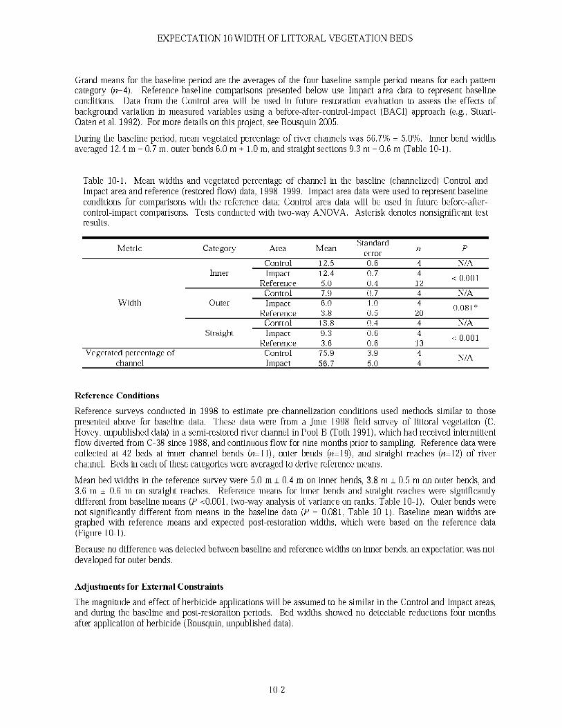
EXPECTATION 10 WIDTH OF LITTORAL VEGETATION BEDS

Grand means for the baseline period are the averages of the four baseline sample period means for each pattern category (n-4). Reference-baseline comparisons presented below use Impact area data to represent baseline conditions. Data from the Control area will be used in future restoration evaluation to assess the effects of background variation in measured variables using a before-after-control-impact (BACI) approach (e.g., Stuart- Oaten et al. 1992). For more details on this project, see Bousquin 2005.

During the baseline period, mean vegetated percentage of river channels was 56.7% ± 5.0%. Inner bend widths averaged 12.4 m ± 0.7 m, outer bends 6.0 m ± 1.0 in, and straight sections 9.3 m ± 0.6 m (Table 10-1).

Table 10-1. Mean widths and vegetated percentage of channel in the baseline (channelized) Control and Impact area and reference (restored flow) data, 1998-1999. Impact area data were used to represent baseline conditions for comparisons with the reference data; Control area data will be used in future before-after- control-impact comparisons. Tests conducted with two-way ANOVA. Asterisk denotes nonsignificant test results.

M etric C ategory A rea M eanStandard

errorn P

C ontrol 12.5 0.6 4 N/AInner Im pact 12.4 0.7 4 < 0 001

R eference 5.0 0.4 12C ontrol 7.9 0.7 4 N/A

W id th O uter Im pact 6.0 1.0 4 0 081*R eference 3.8 0.5 20

C ontrol 13.8 0.4 4 N/AStraight Im pact 9.3 0.6 4 < 0 001

R eference 3.6 0.6 13V egeta ted percen tage o f C ontrol 75.9 3.9 4 N/A

channel Im pact 56.7 5.0 4

Reference Conditions

Reference surveys conducted in 1998 to estimate pre-channelization conditions used methods similar to those presented above for baseline data. These data were from a June 1998 field survey of littoral vegetation (C. Hovey, unpublished data) in a semi-restored river channel in Pool B (Toth 1991), which had received intermittent flow diverted from C-38 since 1988, and continuous flow for nine months prior to sampling. Reference data were collected at 42 beds at inner channel bends (n=ll), outer bends (n=19), and straight reaches («=12) of river channel. Beds in each of these categories were averaged to derive reference means.

Mean bed widths in the reference survey were 5.0 m ± 0.4 m on inner bends, 3.8 m ± 0.5 m on outer bends, and 3.6 m ± 0.6 m on straight reaches. Reference means for inner bends and straight reaches were significantly different from baseline means (P <0.001, two-way analysis of variance on ranks, Table 10-1). Outer bends were not significantly different from means in the baseline data (P - 0.081, Table 10-1). Baseline mean widths are graphed with reference means and expected post-restoration widths, which were based on the reference data (Figure 10-1).

Because no difference was detected between baseline and reference widths on inner bends, an expectation was not developed for outer bends.

Adjustments for External Constraints

The magnitude and effect of herbicide applications will be assumed to be similar in the Control and Impact areas, and during the baseline and post-restoration periods. Bed widths showed no detectable reductions four months after application of herbicide (Bousquin, unpublished data).

10-2

EXPECTATION 10 WIDTH OF LITTORAL VEGETATION BEDS

Mechanism for Achieving Expectation

Restoration of continuous flow through river channels will reduce the width of littoral vegetation beds by mechanical removal of plants, substrate, and floating mats. Widths will be determined by flow regimes that will vary with channel pattern. Initial high flows through the channels will remove much of the floating vegetation.

Means of Evaluation

Following completion of Phase I construction, two years of semiannual sampling will be used to evaluate initial responses to flow restoration. Following this period, post-restoration sampling will continue for at least two years. This schedule assumes normal flow regimes. If needed, sampling will be continued until mat widths have stabilized. Post-restoration sampling methodology will be identical to baseline sampling.

The baseline data were evaluated to estimate statistical power and the sample sizes (numbers of sample periods) needed in the post-restoration period to conduct reliable before-after comparisons. Power was estimated for standard t-tests (one-tailed) using only the Impact area data. Assuming equal or lower variability in the post­restoration data, the changes predicted for bed widths at inner bends and straight reaches will be detectable (if they occur) at a <0.05 and/?<0.1 (power >0.9) with data from three post-restoration sampling periods.

14

12 -

Er 10 H ** 8H

§

I2 -

■ R e fe re n c e (p re -c h a n n e lize d )□ B a s e lin e (c h a n n e lize d )U E x p e c te d (p o s t-res to ra tio n )

A

In n er b en d s S tra ig h t rea ch esC h a n n e l p attern

Figure 10-1. Mean relative cover of littoral bed widths on inner bends and straight reaches of river channel in the baseline and reference littoral vegetation surveys, showing values expected following restoration of flow based on reference data. Error bars indicate ± one standard error of the mean.

Time Course

Initially, sufficiently high flows will be needed to remove mid-channel vegetation and alter mat widths; subsequently, flow must be sustained to maintain these new conditions (Toth et al. 1995). Stabilization of widths is expected to occur within one to three years of backfilling and restored flow, but monitoring will be continued until bed widths stabilize.

10-3

EXPECTATION 10 WIDTH OF LITTORAL VEGETATION BEDS

Literature Cited

Bousquin, S. G. 2005. Littoral vegetation in the channelized Kissimmee River. Chapter 7 in S. G. Bousquin, D. H. Anderson, G. E. Williams, and D. J. Colangelo, editors. Establishing a baseline: pre-restoration studies of the channelized Kissimmee River. South Florida Water Management District, West Palm Beach, Florida, USA. Technical Publication ERA #432.

Stewart-Oaten, A., J. R. Bence, and C. W. Osenburg. 1992. Assessing effects of unreplicated perturbations: no simple solutions. Ecology 73:1396-1404.

Toth, L. A. 1991. Environmental responses to the Kissimmee River Demonstration Project. Technical Publication 91-02. South Florida Water Management District, West Palm Beach, Florida, USA.

Toth, L. A., D. A. Arrington, M. A. Brady, and D. A. Muszick. 1995. Conceptual evaluation of factors potentially affecting restoration of habitat structure within the channelized Kissimmee River ecosystem. Restoration Ecology 3:160-180.

10-4

EXPECTATION 11

PLANT COMMUNITY STRUCTURE IN RIVER CHANNELS

Expectation

Littoral plant community structure will undergo the following changes in restored river channels:(1) Combined mean relative cover of emergent species will increase to >80%.(2) Combined mean relative cover of floating and mat-forming species will decrease to <10%.

Author

Stephen G. Bousquin, South Florida Water Management DistrictCaroline Hovey, South Florida Water Management District (Current affiliation'. Hovey Environmental)

May 11,1999 (Hovey); revised April 2002 (Bousquin); revised December 2004 (Bousquin)

Relevant Endpoints

Sociopolitical-Nuisance (Non-Native) Species Restoration-Biological Integrity-Community Structure Restoration-System Functional Integrity-Habitat Quality

Metrics

Relative cover of emergent speciesRelative cover of floating and mat-forming species

Baseline Conditions

Baseline sampling was conducted twice annually from 1998 to 1999 during the winter dry season (usually February-March) and the summer wet season (August-September) at fixed transects distributed in non-flowing (remnant) channels of Pools A (Control area), and B and C (Impact area). Each transect is permanently marked on opposite banks with galvanized steel poles. Vegetation sampling was conducted in one-meter wide belt transects established by sighting between the transect poles and placing 1 m by 2 m quadrats on the upstream side of the sightline, with the long dimension of the quadrat on the transect. Surveys were initiated at the left bank facing downstream and were continued across the channel by adding consecutive quadrats. For each quadrat, we recorded the overall percentage cover of living and dead vegetation to the nearest 5%, and cover of all plant species using a six-level system developed by Daubenmire (1959). The midpoints of cover classes were used for calculations involving species cover classes (Table 11-1) (Daubenmire 1959). Relative cover was averaged over all sampled vegetated transect sections for each species or growth-form for each of the four baseline sample periods. Grand means for the baseline period are the averages of the four sample period means for each species or growth-form («= 4). For calculations, each transect was subdivided into two transect sections, one for the vegetation bed on either side of the channel. An average of 125 vegetated transect sections occurred per sample period in the Impact area; 42 vegetated transect sections occurred per sample period in the Control area.

11-1

Expectation 11 Plant community structure

Reference-baseline comparisons presented below use Impact area data to represent baseline conditions. Data from the Control area will be used in future restoration evaluation to assess the effects of background variation in measured variables using a before-after-control-impact (BACI) approach (e.g., Stuart-Oaten et al. 1992). For more detail on this project, see Bousquin 2005.

Emergent species and floating/mat-forming species had similar mean relative cover in the baseline period. Of living plant cover, 49.6% ± 4.0% was floating and mat-forming species, 43.3% ± 3.4% was emergent species, and the remainder was submergent and other species (e.g., terrestrial species and taxa identified only to family or genus) (Figure 11-1).

Table 11-1. Reference and baseline mean relative cover for emergents, floating and mat-forming species, and overall living plant cover in the baseline Control and Impact areas and in the reference data. Only Impact area data were used to represent the baseline in comparisons with reference data.

Metric Category Area MeanStandard

errorn P

Control 62.2 4.0 4 N/A

Relative cover (byEmergent Impact

Reference43.395.5

3.42.0

413

< 0.01

growth form) Floating & Mat- ■ forming

Control 34.1 3.9 4Impact

Reference49.64.5

4.02.0

413

< 0.01

Average percentage live plant cover

ControlImpact

59.643.6

4.46.0

44

N/A

(Va:

■ Reference (pre-channelized)□ Baseline (channelized)

Expected (post-restoration)

Emergent Floating & Mat-forming

Growth form

Figure 11-1. Mean relative cover of emergent species and floating and mat-forming species in the Pool B reference data and in the baseline Impact area data. Error bars represent one standard error of the mean.

11-2

Expectation 11 Plant community structure

Relative cover, relative frequency, and importance values (IV, the sum of relative frequency and relative cover) for species with values >5% in any of these three metrics in either or both the baseline and reference data are shown in Table 11-1. Six of the species on this list were floating/mat-forming species, including the tiny floating aquatic fern, Salvinia minima (water spangles), which had the highest IV in the baseline period data. Two other small-leaved floating plants, Wolffiella gladiata (watersprite), and Lemna sp. (duckweed) occurred with lower IV. Also on this list, and present in both data sets, were Eichhomia crassipes (water hyacinth) and Pistia stratiotes (water lettuce); both are floating, invasive exotics, and the only floating species recorded in the reference data. Several floating and mat-forming species were present in the baseline data but not in the reference data, including: Scirpus cubensis, a mat-forming sedge; S. minima; Lemna sp.; and W. gladiata.

Common emergent species in the baseline and reference data were Nuphar lutea (spatterdock), Polygonum densiflorum (smartweed), the native grass Panicum hemitomon (maidencane), Altemanthera philoxeroides (alligatorweed), Hydrocotyle umbellata (pennywort), and the shrub Ludwigia peruviana (Peruvian primrose willow).

Reference Conditions

Reference surveys to estimate pre-channelization conditions used methods similar to those for baseline data. Data to estimate pre-channelization littoral plant community structure were obtained from the Kissimmee River Demonstration Project semi-restored run. Cover class (Daubenmire 1959) data from a field survey of 13 transects in the semi-restored channel (C. Hovey, unpublished data) were used to estimate mean relative cover of plant species under flowing conditions. Relative cover means for the reference field survey are the averages of sampled vegetation beds (two transect sections per transect, n=26) that occurred at the 13 transects.

Emergent species clearly dominated littoral zones in the semi-restored flowing channel. Based on the field survey data, mean combined relative cover of emergents was 95.5% ± 2.0%, and the estimate based on photointerpretation was 97%. Mean combined relative cover of floating and mat-forming species in the field survey was 4.5% ± 1.9%, and 3% in the photointerpretation estimate. Mean relative cover of emergent species and floating and mat-forming species was significantly different between the baseline and reference survey data (P <0.01, Kruskal-Wallis one-way analysis of variance on ranks) (Table 11-2).

Baseline means are graphed with reference means and expected post-restoration cover of emergents and floating and mat-forming species, which were based on the reference data (Figure 11-2).

Table 11-2. Mean relative cover, mean relative frequency, and importance values for all species that occurred with values of > 5% in any of these metrics in the baseline Impact or reference data. Importance is the sum of relative cover and relative frequency.

Relative cover (%) Relative frequency (%) ImportanceForm Code Species Reference (pre- Baseline Reference (pre- Baseline Reference (pre- Baseline

channelized) (channelized) channelized) (channelized) channelized) (channelized)AP01 Altemanthera philoxeroides 0.0 2.1 0.0 5.2 0.0 7.3HU01 Hydrocotyle umbellata 12.5 8.8 18.8 6.8 31.3 15.6LP01 Ludwigia pe nivian a 0.0 3.2 0.0 4.1 0.0 7.3

Emergent NL01 Nuphar lutea 26.4 11.0 20.3 4.2 46.7 15.2PD01 Polygonum densiflorum 35.2 4.7 25.0 4.1 60.2 8.8PH01 Panicum hemitomon 5.5 0.6 9.4 1.4 14.9 2.0SS01 Sacciolepis striata 4.1 8.5 6.3 6.9 10.4 15.4EC01 Eichhorma crassipes 2.5 0.5 4.7 0.8 7.2 1.3LM99 Lemna sp. 0.0 5.5 0.0 7.7 0.0 13.2

Floating & Mat- PS01 Pistia stratiotes 2.0 7.6 4.7 5.3 6.7 12.9forming SC05 Scirpus cubensis 0.0 10.3 0.0 5.5 0.0 15.8

SM01 Salvinia minima 0.0 20.8 0.0 7.7 0.0 28.5WG01 Wolffiella gladiata 0.0 2.9 0.0 5.2 0.0 8.1

11-3

Expectation 11 Plant community structure

AP01

HU01

LP01

{? NL010)LU PD01

PH01

SS01

EC01

□ B aseline (channelized)■ R eference (pre-channelized)

Species

Ul ----------| LM99

£& PS01TO

08 SC05O)cI SM01

WG01

AP01 Altem anthera philoxeroides Em ergentEC01 E ichhornia crassipes Floating & Mat-form ingHU01 H ydrocotyle um bellata Em ergentLM99 Lem na sp. Floating & Mat-form ingLP01 Ludw igia peruviana Em ergentNL01 N uphar lutea Em ergentPD01 Polygonum densiflorum Em ergentPH01 Panicum hemitomon Em ergentPS01 Pistia stratiotes Floating & Mat-form ingSC05 Scirpus cubensis Floating & Mat-form ingSM01 Salvin ia m inima Floating & Mat-form ingSS01 Saccio lep is striata Em ergent

W G01 W olffie lla qladiata Floating & Mat-form ing

10 20 30 40Importance value

50 60 70

Figure 11-2. Common species in baseline (channelized) and reference (flowing) area remnant channels.

Adjustments for External Constraints

The magnitude and effect of herbicide applications will be assumed to be similar in the Control and Impact areas, and during the baseline and post-restoration periods. Bed widths showed no detectable reductions by four months after herbicide application (Bousquin, unpublished data).

Mechanism for Achieving Expectation

Post-restoration changes in plant community structure of littoral zones will be dependent on the return of flow to remnant river channels. Initial high flows will remove much of the mid-channel vegetation. Because most mid­channel species are floating non-native species, this initial flow will cause reductions in cover of both floating/mat-forming species and non-native species. Subsequently, flow must be sustained so that species better suited to continuous flow and varying water levels can become dominant.

The predicted shift to dominance by emergents is not dependent on colonization, because most sampled vegetation mats (>98%) were composed of mixtures of emergents and floating and mat-forming species. The expectation of higher relative cover and dominance of emergent species following restoration also does not

11-4

Expectation 11 Plant community structure

suggest that absolute cover of emergent species will increase. Because relative cover is calculated relative to total vegetation cover, a decrease in the absolute cover of floating and mat-forming species could result in higher relative cover of emergents, even if absolute cover of emergents remains unchanged. Moderate expansion of emergents may take place as channel substrate and cross-sections change; however, the expectation is not dependent on such expansion.

Means of Evaluation

Following completion of Phase I construction, two years of semiannual sampling will be used to evaluate initial responses to flow restoration. Following this period, post-restoration sampling will continue for at least two years, assuming normal flow regimes. If needed, sampling will be continued until bed community structure has stabilized. Post-restoration sampling methodology will be identical to baseline sampling.

The baseline data were evaluated to estimate statistical power and the sample sizes (numbers of sample periods) needed in the post-restoration period to conduct reliable before-after comparisons. Power was estimated for standard t-tests (one-tailed) using only the Impact area data. Assuming equal or lower variability in the post­restoration data, the predicted amounts of change for both emergents and floating and mat-forming species will be detectable (if they occur) at a < 0.05 and j3 < 0.1 (power > 0.9) with two sample periods of restored-condition data.

Time Course

Changes in plant community structure are expected one to three years after backfilling and restored flow (Toth et al. 1995), but monitoring will continue until community structure stabilizes.

Literature Cited

Bousquin, S. G. 2005. Littoral vegetation in the channelized Kissimmee River. Chapter 7 in S. G. Bousquin, D. FI. Anderson, G. E. Williams, and D. J. Colangelo, editors. Establishing a baseline: pre-restoration studies of the channelized Kissimmee River. South Florida Water Management District, West Palm Beach, Florida, USA. Technical Publication ERA #432.

Daubenmire, R. 1959. A canopy coverage method of vegetational analysis. Northwest Science 33:42-64.

Stewart-Oaten, A., J. R. Bence, and C. W. Osenburg. 1992. Assessing effects of unreplicated perturbations: no simple solutions. Ecology 73:1396-1404.

Toth, L. A., D. A. Arrington, M. A. Brady, and D. A. Muszick. 1995. Conceptual evaluation of factors potentially affecting restoration of habitat structure within the channelized Kissimmee River ecosystem. Restoration Ecology 3:160-180.

11-5

EXPECTATION 12

AREAL COVERAGE OF FLOODPLAIN WETLANDS

Expectation

Wetland plant communities will cover >80% of the area of the floodplain restored in Phases I-IV.

Author

Laura Carnal, South Florida Water Management District

March 3,1999; revised October 8, 2002; revised March 2003, February 2005, July 2005

Relevant Endpoints

Sociopolitical - Total Wetland AreaSociopolitical - Nuisance (Exotic) SpeciesRestoration - System Functional Integrity - Habitat Quality

Metrics

Percent of restored area of floodplain covered by wetlands

Baseline Conditions

Early post-channelization vegetation data based on 1973 and 1974 aerial photography (adjusted from Milleson et al. 1980) indicate that wetland vegetation covered approximately 29% of Pools A-D three years after channelization of the Kissimmee River. More recent vegetation mapping of Pool C (Carnal and Bousquin 2005) during the channelized period indicate that the area of wetland plant communities in Pool C was similar in 1996, with coverage of 32% Most wetlands during the channelized period occurred in the lower, impounded portions of pools and in depressions and sloughs (Carnal and Bousquin 2005).

Reference Conditions

Pre-channelization aerial photography (1952-1954) data (adjusted from Pierce et al. 1982) indicate that, prior to channelization, wetland plant communities covered approximately 81% of the floodplain in the restoration and control areas of Pools A-D, 83% of Pool C alone, and 80% of the area slated for restoration in construction Phases I - IV (Table 12-1). The restoration-area pre-channelization data were used to predict the expected minimum of 80% wetland coverage following restoration of flow and inundation.

12-1

EXPECTATION 12 AREAL COVERAGE OF FLOODPLAIN WETLANDS

Adjustments for External Constraints

The River Acres residential community in southeastern Pool D will not be included in the restoration project. This site has an area of approximately 153 ha and was dominated by marsh wetland communities prior to channelization. This area was subtracted from reference condition data to arrive at the 80% wetlands expectation (Figure 12-1).

Table 12-1. Areal coverage of wetlands and other general vegetation categories by restoration phase. The 1952 pre-channelization data (Pierce et al. 1982) were used to predict the expected effect of restoration on wetland area. The 1974 data (Milleson et al. 1980) were used for whole-system channelized-condition (baseline) estimates.

A rea (ha) Percent o f restoration area

Phase Status 1952 1974 1952 1974

A quatic 61 36 0.6 0.3

N on-vegetated 210 561 2.0 5.4

Phase I U nknow n 20 0 0.2 0.0

U pland 402 2414 3.8 23.1

W etland 3154 836 30.1 8.0

A quatic 115 68 1.1 0.7

N on-vegetated 461 961 4.4 9.2

Phase II/III U nknow n 17 1 0.2 0.0

U pland 389 2019 3.7 19.3

W etland 3405 1337 32.5 12.8

A quatic 25 50 0.2 0.5

N on-vegetated 120 219 1.1 2.1

Phase IV U nknow n 6 0 0.1 0.0

U pland 186 661 1.8 6.3

W etland 1354 761 12.9 7.3

A quatic 8 12 0.1 0.1

N on-vegetated 65 122 0.6 1.2

Phase IVA U nknow n 2 0 0.0 0.0

U pland 33 185 0.3 1.8

W etland 439 228 4.2 2.2

G rand Total 10472 10472 100 100

Mechanism for Achieving Expectation

Backfilling of the C-38 canal and implementation of the new headwaters regulation schedule (Bousquin et al. 2005) will reestablish depth, extent, duration, and frequency of floodplain inundation. Historic floodplain inundation regimes will create conditions favorable for wetland vegetation. Wetland vegetation will colonize flooded habitat through seed dispersal and vegetative reproduction of remnant communities, and from germination of viable remnant seed banks. Increased inundation of the floodplain will rapidly eliminate upland species that are intolerant of flooding. Evidence that such a shift will take place was observed in Rattlesnake Hammock Marsh, a 228 ha impoundment in the Pool A floodplain that was created in 1990 and subjected to

1 2 - 2

EXPECTATION 12 AREAL COVERAGE OF FLOODPLAIN WETLANDS

increased hydroperiods in the early 1990s (Toth et al. 1998). The coverage of wetland communities in the impoundment increased from virtually zero following channelization (Milleson et al. 1980) to >40% by 1996, including 80 ha of broadleaf marsh and 14 ha of wet prairie (L. Carnal, SFWMD, unpublished data).

Means of Evaluation

Total floodplain wetland area will be tracked for each phase of the project at three-5 year intervals after reestablishment of historic floodplain hydroperiod characteristics. After Phase I of restoration (most of Pool C and lower Pool B), wetland communities should eventually cover approximately 3154 ha (30%) of the 10,472 ha area encompassed by all phases of restoration. Phase II/III (most of Pool D and lower Pool C) will restore an additional 3405 ha (33%) in the restoration area. Following Phase IV (two additional sections of lower Pool B), an additional 1793 ha of wetlands or 17% of the total restored area will be added, for a cumulative total restored wetland area of 8352 ha or approximately 80% of the restoration area.

10090

R eference (p re - Baseline Expected minimumchannelization) (channelized)

Figure 12-1. Pre-channelized, channelized, and expected percentages of wetland vegetation in the restoration project area.

Aerial photography will be acquired, interpreted, converted to digital map data, and georeferenced to produce a seamless vegetation map. Ground truth data will be collected simultaneously for use in signature calibration and accuracy assessment. The mapped vegetation data will be used to calculate the areal coverage of each classified community and to detect changes in area. Total wetland area will be compared to the adjusted reference values, which were derived from the pre-channelization (1952-1954) vegetation map of Pierce et al. (1982). The expectation will be achieved when the percentage of wetland area on the restored portion of Pools B, C, and D meet or exceed the predicted values. Satellite image data may be acquired and interpreted to assess intermediate change with lower resolution than aerial photography. Aerial photography acquired for each phase of the restoration project will include Pool A (north of the restoration area), which will serve as a channelized-condition control site. While plant communities on small portions of the Pool A floodplain may change in response to restoration project activities (e.g., backfilling of local agricultural ditches, breaching the tie-back levee between Pools A and B to allow sheet flow on the floodplain), such changes will be taken into account during evaluations.

Time Course

Reestablishment of >80% coverage of floodplain wetland plant communities in the restored areas of Pools B, C, and D will take four to five years after the following two requirements have been met. First, the backfilling of the C-38 canal must be completed for all restoration phases, and second, the headwaters revitalization stage regulation schedule, which will mimic historic hydroperiods (Bousquin et al. 2005, Williams et al. 2005), must be implemented.

12-3

EXPECTATION 12 AREAL COVERAGE OF FLOODPLAIN WETLANDS

The rate of change in plant communities will be linked closely to hydrologic conditions in the years following backfilling (Toth et al. 1995). If the floodplain experiences extended drought conditions in the early years of recovery, or the new regulation schedule does not restore historic hydrology, it is likely that upland herbaceous and shrub species will persist in areas where wetland species are expected to reestablish. These upland species will decline when normal climatic conditions return and historic hydrology is restored.

Literature Cited

Bousquin, S. G., D. H. Anderson, D. J. Colangelo, and G. E. Williams. 2005. Introduction: baseline studies of the channelized Kissimmee River. Chapter 1 in S. G. Bousquin, D. H. Anderson, G. E. Williams, and D. J. Colangelo, editors. Establishing a baseline: pre-restoration studies of the channelized Kissimmee River. South Florida Water Management District, West Palm Beach, Florida, USA. Technical Publication ERA #432.

Carnal, L. L., and S. G. Bousquin. 2005. Areal coverage of floodplain plant communities in Pool C of the channelized Kissimmee River. Chapter 10 in S. G. Bousquin, D. H. Anderson, G. E. Williams, and D. J. Colangelo, editors. Establishing a baseline: pre-restoration studies of the channelized Kissimmee River. South Florida Water Management District, West Palm Beach, Florida, USA. Technical Publication ERA #432.

Milleson, J. F., R. L. Goodrick, and J. A. Van Arman. 1980. Plant communities of the Kissimmee River valley. Technical Publication 80-7. South Florida Water Management District, West Palm Beach, Florida, USA.

Pierce, G. J., A. B. Amerson, and L. R. Becker. 1982. Final report: pre-1960 floodplain vegetation of the lower Kissimmee River valley, Florida. Biological Services Report 82-3. U. S. Army Corps of Engineers, Jacksonville, Florida, USA.

Toth, L. A., S. L. Melvin, D. A. Arrington, and J. Chamberlain. 1998. Hydrologic manipulations of the channelized Kissimmee River. BioScience 48:757-764.

Toth, L. A., D. A. Arrington, M. A. Brady, and D. A. Muszick. 1995. Conceptual evaluation of factors potentially affecting restoration of habitat structure in the channelized Kissimmee River ecosystem. Restoration Ecology 3:160-180.

Williams, G. E., J. W. Koebel, D. H. Anderson, S. G. Bousquin, D. J. Colangelo, J. L. Glenn, B. L. Jones, C. Carlson, L. Carnal, and J. Jorge. 2005. Kissimmee River Restoration and Upper Basin Initiatives. Chapter 11 in South Florida Environmental Report Volume I: The South Florida Environment - Water Year 2004. South Florida Water Management District, West Palm Beach, Florida, USA, and Florida Department of Environmental Protection, Tallahassee, Florida, USA. Technical Publication ERA #432.

12-4

EXPECTATION 13

AREAL COVERAGE OF BROADLEAF MARSH

Expectation

Broadleaf Marsh will cover at least 50% of the restored floodplain in Pools B, C, and D.

Author

Laura Carnal, South Florida Water Management District

June 6,1998; revised October 8, 2002; revised March 2003; revised February 2005

Relevant Endpoints

Ecological Integrity/Sociopolitical - Total Wetland AreaRestoration - System Functional Integrity - Habitat Quality - Habitat Diversity

Metrics

Percent of restored floodplain area covered by Broadleaf Marsh

Baseline Conditions

Early post-channelization data (adjusted from Milleson et al. 1980) based on 1973 and 1974 aerial photography indicate that Broadleaf Marsh (BLM) communities (defined in Bousquin and Carnal 2005) covered 10% of the 10,472 ha area that will be affected by Phases I-IV of restoration.

Reference Conditions

Pre-channelization (1952-1954) data (adjusted from Pierce et al. 1982) indicate that BLM covered approximately 49% of the area that will be affected by all phases of the restoration project (Table 13-1). The pre-channelization restoration-area data, adjusted as described below, were used as reference conditions to obtain the value of 50% BLM coverage predicted by this expectation.

Adjustments for External Constraints

MacArthur Impoundment was constructed prior to the historical photography used by Pierce et al. (1982) to map pre-channelization vegetation. This 600 ha system of levees and ditches was created to drain wetlands for use as cattle pasture. The impoundment likely shortened hydroperiods, creating favorable conditions for wet prairie communities in the southern end of the impoundment and upland species in the northern end. Because the

13-1

EXPECTATION 13 AREAL COVERAGE OF BROADLEAF MARSH

surrounding area was historically dominated by broadleaf, it is likely that BLM associations will reestablish in the area after the ditches and levees are removed and hydrology is restored. The area of the impoundment occupied by maidencane (.Panicum hemitomon) Wet Prairie (425 ha) prior to channelization was added to the reference condition value to adjust the expected value. The River Acres residential community in southeastern Pool D will not be included in the restoration project. This site has an area of approximately 153 ha and was historically dominated by BLM and Wet Prairie communities. This area was subtracted from the adjusted reference condition value.

Based on these adjustments, BLM communities are expected to increase incrementally with each phase of restoration. Following Phase I, BLM is expected to occur on approximately: 20% of the area affected by the restoration in Pools B, C, and D (adjusted for MacArthur Impoundment); an additional 22% following Phase II/III (adjusted for River Acres); and an additional 9% following Phase IV, for a cumulative total of approximately 51% of the area affected by the project. This expectation will be achieved when the total areal coverage of BLM in restored portions of Pools B, C, and D is at least 50% (Figure 13-1).

Table 13-1. Areal coverage and percentages of Broadleaf Marsh prior to channelization (1952) and three years after channelization (1974) in the areas to be restored in restoration Phases I-IV.

Area (ha) by yearPercent of restoration area

(10,472 ha) by yearRestoration phase 1952 1974 1952 1974

Phase I 1672 175 16.0 1.7Phase II/III 2504 565 23.9 5.4

Phase IV 674 124 6.4 1.2Phase IVA 256 190 2.4 1.8

Totals 5106 1054 49 10

Mechanism for Achieving Expectation

Backfilling of the C-38 canal and implementation of the interim and new headwaters stage regulation schedule will reestablish historic floodplain inundation characteristics of depth, extent, duration, and frequency (Bousquin et al. 2005). Prolonged floodplain inundation regimes will create conditions favorable for BLM vegetation (Toth et al.1995). Broadleaf marsh species will colonize flooded habitat through seed dispersal, vegetative growth from remnant communities, and from germination of remnant seed banks. A similar shift from pasture to BLM was observed in Rattlesnake Hammock Marsh, a 228 ha impoundment in Pool A, which was created in 1990 and subjected to increased hydroperiods in the early 1990s (Toth et al. 1998). Broadleaf Marsh communities increased from virtually zero coverage following channelization (Milleson et al. 1980) to approximately 80 ha by 1996 (L. Carnal, SFWMD, unpublished data). Following restoration, most areas that are currently pasture are expected to revert to BLM. However, the established pasture grasses are adapted to periodic wet conditions, so consistently long hydroperiods are needed to displace bahia grass (Paspalum notatum) and bermuda grass (Cynodon dactylon). C-38 and areas that are currently occupied by spoil will experience successional phases and eventually will be colonized by BLM species.

Means of Evaluation

The areal coverage of BLM will be tracked in three-5 year intervals after reestablishment of historic floodplain hydroperiod characteristics for each phase of the project. Aerial photography will be acquired, interpreted, converted to digital map data, and georeferenced to produce a seamless vegetation map. Ground truth data will be collected simultaneously for use in signature calibration and accuracy assessment. The mapped vegetation

13-2

EXPECTATION 13 AREAL COVERAGE OF BROADLEAF MARSH

data will be used to calculate the areal coverage of each classified community and to detect changes in areal extent of communities. Total BLM area will be compared with the adjusted reference values for each restoration phase. Satellite image data may be acquired and interpreted to provide additional vegetation data to assess intermediate change.

Aerial photography will include Pool A, which will not be backfilled and serves as a control site. While Pool A vegetation floodplain may experience some change in response to restoration-related activities (e.g., backfilling of local agricultural ditches, breaching the tie-back levee between Pools A and B to allow sheet flow on the floodplain), these changes will be taken into account in evaluations. Changes in each phase of the project will be evaluated by comparing vegetation map data for the baseline period with post restoration data, relative to the Pool A control.

100 1----------------------------------------------------------------------------------------9 0 ----------------------------------------------------------------------------------------------------------

8 0 ----------------------------------------------------------------------------------------------------------

| 70 ro5 60

R eference (p re - B a s e lin e (c h a n n e lize d ) E xp e c te d m in im u mch a n n e liza tio n )

Figure 13-1. Pre-channelization, channelized, and expected percentages of Broadleaf Marsh in the restoration project area.

Time Course

Two requirements are necessary to achieve this expectation. First, backfilling of the C-38 canal must be completed for all restoration phases, and second, implementation of the headwaters revitalization stage regulation schedule, which will mimic historic hydroperiods (Bousquin et al. 2005) must take place. However, the rate of transition in vegetation communities will be linked closely to the hydrologic conditions in the years following backfilling (Toth et al. 1995). If the floodplain experiences extended drought conditions in the early years of recovery, or the interim regulation schedule does not reestablish historic inundation regimes, it is likely that upland weeds, shrubs, and pasture grasses will persist on the floodplain and impede reestablishment of BLM species. These upland species will decline when normal climatic conditions return and historic hydrology is restored.

Literature Cited

Bousquin, S. G., D. H. Anderson, D. J. Colangelo, and G. E. Williams. 2005. Introduction: baseline studies of the channelized Kissimmee River. Chapter 1 in S. G. Bousquin, D. H. Anderson, G. E. Williams, and D. J. Colangelo, editors. Establishing a baseline: pre-restoration studies of the channelized Kissimmee River. South Florida Water Management District, West Palm Beach, Florida, USA. Technical Publication ERA#432.

13-3

EXPECTATION 13 AREAL COVERAGE OF BROADLEAF MARSH

Bousquin, S. G., and L. L. Carnal. 2005. Classification of the vegetation of the Kissimmee River and floodplain. Chapter 9 in S. G. Bousquin, D. H. Anderson, G. E. Williams, and D. J. Colangelo, editors. Establishing a baseline: pre-restoration studies of the channelized Kissimmee River. South Florida Water Management District, West Palm Beach, Florida, USA. Technical Publication ERA #432.

Milleson, J. F., R. L. Goodrick, and J. A. Van Arman. 1980. Plant communities of the Kissimmee River valley. Technical Publication 80-7. South Florida Water Management District, West Palm Beach, Florida, USA.

Pierce, G. J., A. B. Amerson, and L. R. Becker. 1982. Final Report: pre-1960 floodplain vegetation of the lower Kissimmee River Valley, Florida. Biological Services Report 82-3. U. S. Army Corps of Engineers, Jacksonville, Florida, USA.

Toth, L. A., S. L. Melvin, D. A. Arrington, and J. Chamberlain. 1998. Hydrologic manipulations of the channelized Kissimmee River. BioScience 48:757-764.

Toth, L. A., D. A. Arrington, M. A. Brady, and D. A. Muszick. 1995. Conceptual evaluation of factors potentially affecting restoration of habitat structure within the channelized Kissimmee River ecosystem. Restoration Ecology 3:160-180.

13-4

EXPECTATION 14

AREAL COVERAGE OF WET PRAIRIE

Expectation

Wet Prairie communities will cover at least 17% of the floodplain restored by Phases I-IV of the restoration project.

Author

Laura Carnal, South Florida Water Management District

May 25,1999; revised October 28, 2002; revised March 2003; revised February 2005

Relevant Endpoints

Sociopolitical - Total Wetland AreaRestoration - System Functional Integrity - Habitat Quality - Habitat Diversity

Metrics

Percent of restored floodplain area covered by Wet Prairie

Baseline Conditions

Early post-channelization data (adjusted from Milleson et al. 1982) indicate that in 1973 and 1974, three years after channelization was completed, Wet Prairie communities (defined in Bousquin and Carnal 2005) covered approximately 11% of the area to be restored in Phases I-IV (10,472 ha ) of the Kissimmee River Restoration Project (Table 14-1).

Reference Conditions

Pre-channelization data based on mapping of 1952 to 1954 aerial photography (adjusted from Pierce et al. 1982), indicate that Wet Prairie communities comprised approximately 22% of the areas of Pools B-D slated for restoration in construction Phases I-IV (Table 14-1). These pre-channelization restoration-are a data, adjusted as described below, were used as reference conditions for predicting post-restoration recovery of Wet Prairie to 17% of the restored system.

Adjustments for External Constraints

Historical reference condition data are based on aerial photography taken after MacArthur Impoundment was constructed. This system of levees and ditches was created to drain wetlands for pasture use, and likely shortened hydroperiods. This created favorable conditions for Wet Prairie species in the southern end of the impoundment

14-1

EXPECTATION 14 AREAL COVERAGE OF WET PRAIRIE

and upland pasture species in the northern end. Historic vegetation data (Pierce et al. 1982) show expanses (425 ha) of Panicum hemitomon (maidencane) that occurred in MacArthur Impoundment. Because the surrounding area was historically dominated by Broadleaf Marsh species, maidencane is not expected to remain in this area after the ditches and levees have been degraded. Therefore, the 425 ha of maidencane within the impoundment was subtracted from reference condition data. The River Acres residential community in southeastern Pool D will not be included in the restoration project. This site has an area of approximately 153 ha and was historically dominated by Broadleaf Marsh and Wet Prairie communities. This area has also been subtracted from reference condition data.

Based on these adjustments, Wet Prairie is expected to cover: 7% of the floodplain affected by Phase I; 3% of that affected by Phase II/III; and 6% of that affected by Phase IV, for a cumulative total of 17% expected cover in the restoration area. This expectation will be achieved when Wet Prairie communities cover at least 17% of the total floodplain area in the Phase I-IV restoration area (Figure 14-1).

Table 14-1. Areal coverage and percentages of Wet Prairie prior to channelization (1954) and three years after channelization (1974) in the areas to be restored during restoration Phases I-IV.

Area (ha)Percent of restoration area

(10,472 ha)1952 1974 1952 1974

Phase I 1185 525 11.3 5.0Phase II/III 515 182 4.9 1.7

Phase IV 471 402 4.5 3.8Phase IVA 179 17 1.7 0.2

Totals 2350 1125 22 11

Mechanism for Achieving Expectation

Backfilling of the C-38 canal, and implementation of the interim and new headwaters stage regulation schedules (Bousquin et al. 2005), will reestablish floodplain inundation characteristics (depth, extent, duration, and frequency). Historic floodplain inundation regimes will create conditions favorable for growth and reproduction of Wet Prairie species. Wet Prairie species will colonize through seed dispersal and vegetative reproduction of remnant communities, and from germination of remnant seed banks. Wet Prairie associations will reestablish along the periphery of the floodplain and on the higher elevations within Broadleaf Marsh communities where annual hydroperiods range from three to eight months with depths <25 cm. Reestablishing longer hydroperiods will eventually eliminate upland species that are less tolerant of fluctuating water depths and periods of inundation. A shift from pasture to Wet Prairie communities was measured in Rattlesnake Hammock Marsh, a 228 ha impoundment in the Pool A floodplain that was created in 1990 and subjected to fluctuating water levels (Toth et al. 1998). Wet Prairie communities were virtually absent following channelization (Milleson et al. 1980) and increased to 14 ha by 1996 (L. Carnal, SFWMD, unpublished data).

Means of Evaluation

The areal coverage of Wet Prairie will be tracked in three-5 year intervals after reestablishment of historic floodplain hydroperiod characteristics for each phase of the project. Aerial photography will be acquired, interpreted, converted to digital map data, and georeferenced to produce a seamless vegetation map. Ground truth data will be collected simultaneously for use in signature calibration and accuracy assessment. The mapped vegetation data will be used to calculate the areal coverage of each classified community and to detect changes in area. Wet Prairie communities will be determined by dominance of diagnostic species (Bousquin and Carnal 2005). Wet Prairie includes 14 community types (Bousquin and Carnal 2005) with vegetation cover that is dominated by: diagnostic wetland

14-2

EXPECTATION 14 AREAL COVERAGE OF WET PRAIRIE

grasses, such as Panicum hemitomon and Luziolafluitans', forbs, such as Polygonum punctatum and Iris virginica, or sedges such as Juncus effusus and Cyperus spp.). Polygons that contain transitional plant mixtures will be field- verified to ascertain the correct community association. Total Wet Prairie area will be compared with the adjusted reference values. Post-restoration Wet Prairie floodplain coverage will be overlaid on the historic Wet Prairie coverage to determine differences in distribution, and to calculate percent overlap of cover.

For each phase of the project, changes in the area of Wet Prairie communities in the restored reach will be evaluated by comparing the changes from the baseline period to the post restoration period relative to those in the Pool A control. While vegetation communities on a portion of the Pool A floodplain may change in response to altered hydrology caused by the restoration project (e.g., backfilling of local agricultural ditches, breaching the tie-back levee between Pools A and B to allow sheet flow on the floodplain), these changes will be taken into account during the analysis.

100 1-----------------------------------------------------------------------------------jjj 9 0CO 8 0 ---------------------------------------------------------------------------------------------------------------------------------

.1 7 0 -----------------------------------------------------------------------------------------------------------------------------------

I 6 0 --------------------------------------------------------------------------------------------------1 5 0 -----------------------------------------------------------------------------------------------------------------------------------

T5 40

Reference (pre- Baseline (channelized) Expected minimum channelization)

Figure 14-1. Pre-channelization, channelized, and expected percentages of Wet Prairie in the restoration project area. Reference conditions were adjusted downward in deriving the expectation because two former areas of Wet Prairie are not expected to succeed to Wet Prairie in the restored system (see text).

Time Course

Two requirements are necessary to achieve this expectation. First, completion of C-38 backfilling for each restoration phase must occur, and second, the implementation of the headwaters revitalization stage regulation schedule, which will mimic historic hydroperiods (Williams et al. 2005), must take place. Within three growing seasons after historic hydroperiods are restored, some areas of the floodplain should reflect dominance by Wet Prairie species. However, these species cannot tolerate prolonged hydroperiods where water levels exceed 25 cm. As the floodplain experiences consistent inundation, there may be a short period when the areal coverage of Wet Prairie declines until it reestablishes at higher elevations and more favorable water levels. This expectation should be achieved within four years, once historic hydroperiods are reestablished for each phase of the project.

The rate of transition of the vegetation communities will be linked closely to the hydrologic conditions in the years following backfilling (Toth et al. 1995). If the floodplain experiences extended drought conditions in the early years of recoveiy, or the interim regulation schedule does not reestablish suitable inundation regimes (three to eight month hydroperiod), it is likely that upland weeds, shrubs, and pasture grasses will persist in areas where Wet Prairie species are expected to reestablish. These upland species will decline when normal climatic conditions return and historic hydrology is restored.

14-3

EXPECTATION 14 AREAL COVERAGE OF WET PRAIRIE

Literature Cited

Bousquin, S. G., D. H. Anderson, D. J. Colangelo, and G. E. Williams. 2005. Introduction: baseline studies of the channelized Kissimmee River. Chapter 1 in S. G. Bousquin, D. H. Anderson, G. E. Williams, and D. J. Colangelo, editors. Establishing a baseline: pre-restoration studies of the channelized Kissimmee River. South Florida Water Management District, West Palm Beach, Florida, USA. Technical Publication ERA #432.

Bousquin, S. G., and L. L. Carnal. 2005. Classification of the vegetation of the Kissimmee River and floodplain. Chapter 9 in S. G. Bousquin, D. H. Anderson, G. E. Williams, and D. J. Colangelo, editors. Establishing a baseline: pre-restoration studies of the channelized Kissimmee River. South Florida Water Management District, West Palm Beach, Florida, USA. Technical Publication ERA #432.

Milleson, J. F., R. L. Goodrick, and J. A. Van Arman. 1980. Plant communities of the Kissimmee River Valley. Technical Publication 80-7. South Florida Water Management District, West Palm Beach, Florida, USA.

Pierce, G. J., A. B. Amerson, and L. R. Becker Jr. 1982. Pre-1960 floodplain vegetation of the lower Kissimmee River Valley, Florida. Biological Services Report 82-3. U. S. Army Corps of Engineers, Jacksonville, Florida, USA.

Toth, L. A., D. A. Arrington, M. A. Brady, and D. A. Muszick. 1995. Conceptual evaluation of factors potentially affecting restoration of habitat structure within the channelized Kissimmee River ecosystem. Restoration Ecology 3:160-180.

Toth, L. A., S. L. Melvin, D. A. Arrington, and J. Chamberlain. 1998. Hydrologic manipulations of the channelized Kissimmee River. BioScience 48:757-764.

Williams, G. E., J. W. Koebel, D. H. Anderson, S. G. Bousquin, D. J. Colangelo, J. L. Glenn, B. L. Jones, C. Carlson, L. Carnal, and J. Jorge. 2005. Kissimmee River Restoration and Upper Basin Initiatives. Chapter 11 in South Florida Environmental Report Volume I: The South Florida Environment - Water Year 2004. South Florida Water Management District, West Palm Beach, Florida and Florida Department of Environmental Protection, Tallahassee, Florida, USA.

14-4

EXPECTATION 15

RIVER CHANNEL MACRO INVERTEBRATE DRIFT COMPOSITION

Expectation

Macroinvertebrate drift composition will be dominated by Coleoptera, Diptera, Ephemeroptera, and Trichoptera.

Author

Joseph W. Koebel Jr., South Florida Water Management District

August 4, 1998; Revised October 20, 2005

Relevant Endpoints

Restoration - System Functional Integrity - Habitat Quality

Metrics

Percent of drift accounted for by Coleoptera Percent of drift accounted for by Diptera Percent of drift accounted for by Ephemeroptera Percent of drift accounted for by Trichoptera

Baseline Condition

Aquatic invertebrate drift samples were collected quarterly from remnant channels of Pool A and C beginning in January 1998. Two drift nets (0.1 m2 equipped with 125 pm mesh netting) were placed 15 cm below the water surface and 0.5 m above the substrate at three locations within each of three remnant river channels in Pool A and C. Samples were collected at 8-hour intervals (+ 1 hour) over a 24-hour period. Current velocity at each surface and bottom net opening, wind direction, and wind velocity were measured whenever a net was set or removed. All samples were preserved in the field with 10% buffered formalin stained with rose bengal.

Macroinvertebrate taxa, including, Coleoptera, Diptera, Ephemeroptera, and Odonata, comprise <1% of total drift density and 23-29% of total drift biomass in Pools A and C. Macro- and microcrustaceans accounted for approximately 97-99% of total drift density and 54-56% of total drift biomass in Pools A and C. Miscellaneous taxa (Hemiptera, Trichoptera, Lepidoptera, Collembola, Gastropoda, Nematoda, and Oligochaeta), comprised <1% and <3% of remaining drift numbers in Pool A and C, respectively. Miscellaneous taxa accounted for approximately 16% and 22% of total drift biomass in Pool A and C, respectively. This is very different from free- flowing southeastern Coastal Plain blackwater rivers, where larval Coleoptera, Diptera, Ephemeroptera, and Trichoptera are the major contributors to drift numbers and biomass.

15-1

EXPECTATION 15 MACROINVERTEBRATE DRIFT

Reference Condition

Historical data on aquatic invertebrate drift composition within the Kissimmee River are unavailable. Reference conditions have been developed based on invertebrate drift data from two unregulated, sixth-order southeastern Coastal Plain rivers, the Satilla and Ogeechee Rivers, Georgia (Benke et al. 1986, 1991). These studies indicate larval Coleoptera, Diptera, Ephemeroptera, and Trichoptera are the major contributors to drift numbers and biomass (Table 15-1). Because these groups of organisms likely were abundant in the pre-channelized Kissimmee River, it is likely that they accounted for the greatest proportion of aquatic invertebrate drift density and biomass. Therefore, aquatic invertebrate drift composition should provide a reliable indicator of restored hydrology and aquatic invertebrate community structure within the river channel. Following restoration of flow, invertebrate drift density and biomass should be dominated by macroinvertebrates (primarily Coleoptera, Diptera, Ephemeroptera, and Trichoptera).

Adjustments For External Constraints

None.

Mechanism for Achieving Restoration

Reestablishment of an aquatic macroinvertebrate community typical of unmodified southeastern Coastal Plain river/floodplain ecosystems is a prerequisite for reestablishing invertebrate drift composition typical of southeastern, blackwater river systems. Restoration of continuous flow and in-channel habitat structure will be the impetus for macroinvertebrate colonization of restored habitats. Colonization by most river channel macroinvertebrate taxa likely to be found in the drift will occur through adult oviposition.

Restored seasonal, variable flow patterns are expected to reestablish macroinvertebrate drift composition typical of unmodified southeastern Coastal Plain rivers, primarily through behavioral (i.e., periodic, for example, to escape from a predator) and constant (i.e., continuous background drift due to accidental dislodgement) drift mechanisms.

Table 15-1. Major invertebrate groups found in the drift of the Satilla and Ogeechee Rivers, Georgia (Benke et al. 1986, 1991) and Pool C of the channelized Kissimmee River. There was no significant difference between invertebrate drift numbers or biomass between Pools A and C; therefore, only Pool C data is presented. Numbers indicate frequency of occurrence.

Satilla River O geechee River Kissimmee River(Pool C)

Taxonom ic G roup D ensity Biom ass Density Biom ass D ensity Biomass

D iptera 52.9 53.8 27.3 10.6 < 1 11.2C oleoptera 11.3 21.5 6.2 27.4 < 1 2.5E phem eroptera 5.8 6.2 15.4 34.6 < 1 7.4T richoptera 18.6 13.8 11.5 20.2 - -O donata 1.4 4.6 1 5.3 <1 2.4C rustacea* 10 < 1 31.9 1.9 96.8 54.6M iscellaneous — — 6.7 — 2.7** 21.9**

* Includes m acro- and m icrocm staceans.** Includes H em iptera, T richoptera, M egaloptera, Lepidoptera, Collem bola, G astropoda, O ligochaeta, andN em atoda.

Means of Evaluation

Invertebrate drift will be sampled monthly beginning two years after implementation of the revised headwaters regulation schedule. A modified baseline sampling procedure will be used for post-construction restoration

15-2

EXPECTATION 15 MACROINVERTEBRATE DRIFT

evaluation. Three samples will be collected for four hours beginning at dusk using 31 cm X 31 cm drift nets equipped with 125 ]um netting facing into the direction of flow, at depths 15 cm below the water surface and 0.5 m above the channel substrate. Because of potential differences in current velocity at the surface and bottom of the water column, nets at each of these locations will provide a better estimate of total water column drift rates. Surface and bottom nets will be placed at three randomly selected locations within reconnected river channels in Pool C, and one randomly selected location in each of three remnant channels in Pool A. Current velocity (m/s) will be measured at each net opening when nets are deployed and retrieved to determine mean current velocity and volume of water sampled. Samples will be analyzed for invertebrate taxonomic composition. Macroinvertebrate drift will be measured for at least two consecutive years. Macroinvertebrate drift composition will be compared to the baseline condition and stated expectation.

Time Course

Colonization of river channel habitats by macroinvertebrates typical of unmodified southern Coastal Plain rivers likely will occur within 6 to 12 months following implementation of the interim upper basin regulation schedule. However, the interim regulation schedule does not provide the consistent and predictable inflow characteristics of the revised headwaters schedule. The unpredictable nature of the interim regulation schedule may have impacts on aquatic invertebrate community structure within reconnected river channels due to periods of no flow, extreme flow, and low levels of dissolved oxygen. Therefore, macroinvertebrate drift composition will be determined after implementation of the revised schedule. This should allow macroinvertebrate composition within the river channel to stabilize, resulting in less variable drift composition.

Literature Cited

Benke, A. C., R. J. Hunter, and F. K. Parrish. 1986. Invertebrate drift dynamics in a subtropical blackwater river. Journal of the North American Benthological Society 5:173-190.

Benke, A. C., K. A. Parsons, and S. M. Dhar. 1991. Population and community patterns of invertebrate drift in an unregulated Coastal Plain river. Canadian Journal of Fisheries and Aquatic Sciences 48:811-823.

15-3

EXPECTATION 16

INCREASED RELATIVE DENSITY, BIOMASS, AND PRODUCTION OF PASSIVE FILTERING-COLLECTORS ON RIVER CHANNEL SNAGS

Expectation

The passive filtering-collector guild will account for the greatest proportion of mean annual density, mean annual biomass, and mean annual snag-dwelling macroinveitebrate production.

Author

Joseph W. Koebel Jr., South Florida Water Management District

March 10,1999; Revised May 2, 2005

Relevant Endpoints

Restoration - Biological Integrity - Community Structure Restoration - Biological Integrity - Food Web Structure Restoration - Biological Integrity - Productivity Restoration - System Functional Integrity - Habitat Quality Restoration - System Functional Integrity - Habitat Use Restoration - System Functional Integrity - Energy Flow Dynamics

Metrics

Percent of annual density accounted for by passive filtering-collectors Percent of annual biomass accounted for by passive filtering-collectors Percent of annual production accounted for by passive filtering-collectors

Baseline Conditions

Snag samples were collected from remnant river channels quarterly between August 1995 and May 1997. Passive filtering-collectors accounted for only 2-3% of mean annual density, 1% of mean annual biomass, and 2-3% of mean annual production in Pools A and C (Figure 16-1).

Reference Conditions

Historical data on the composition, mean annual density, mean annual biomass, and mean annual production of the snag-dwelling, passive filtering-collector macroinveitebrate guild are not available for the Kissimmee River. The primary source of information on aquatic invertebrate community structure and production on snags within the pre-channelized Kissimmee River have been derived from published data on functional feeding group composition, density, biomass, and annual production of snag-dwelling invertebrates in the Satilla River

16-1

EXPECTATION 16 PASSIVE FILTERING COLLECTORS

(Georgia). The Satilla is a sixth-order, southeastern Coastal Plain blackwater river with similar physical, chemical, and hydrologic patterns as the historic Kissimmee River (Benke et al. 1984). Although species composition on snags may differ between systems, similar physical and chemical characteristics should result in similar patterns of invertebrate abundance, standing stock biomass, production, and functional feeding group composition. Filtering-collectors were selected as an indicator guild because they often account for the largest proportion of mean annual density, biomass, and production on snags in southeastern river systems. Additionally, intolerant taxa (e.g., filtering-collector caddisflies) often respond predictably (decrease) to increased perturbation (e.g., no flow, low dissolved oxygen) (Lenat 1988, Lamberti and Berg 1995, Barbour et al. 1996).

Within the Satilla River, passive filtering-collectors accounted for 75-80% of total numbers, 65-75% of total biomass, and 72-79% of total production at two sample locations (Benke et al. 1984) (Figure 16-1). Based on the low baseline estimates for these metrics in the Kissimmee River (Figure 16-1), it is likely that an increase in abundance, biomass, and production of passive filtering-collectors will be an excellent indicator of improved habitat quality and restoration of biotic integrity.

Adjustment for External Constraints

Mechanism for Achieving Restoration

Continuous, variable flow within reconnected river channels will be the impetus for colonization, persistence, and increased productivity of snag-dwelling passive filtering-collectors. Because most passive filtering-collectors are sedentary and utilize various sieving mechanisms for removing particulate matter from suspension, continuous flows are necessary to transport fine particulate organic matter that can be captured and used as a food source. The potential for high standing stock biomass of several filtering-collector taxa (primarily Trichoptera) and rapid biomass turnover rates for others (e.g., Simuliidae and filtering chironomids) likely will result in the greatest proportion of mean annual density, biomass, and production being attributed to filtering-collectors.

70

60

a 50O<3

Oh 40

30

20

10

0Pool A Pool C Site 2

□ Density ■ Biomass□ Production

Figure 16-1. Mean annual density, biomass, and production of passive filtering-collectors on snags in the Kissimmee River (Pools A and C), and Satilla River, Georgia (Sites 1 and 2) (Benke et al. 1984).

Means of Evaluation

Sampling of existing snag habitat will commence approximately six months following initiation of the interim upper basin regulation schedule (January 2001) and reestablishment of continuous flow through reconnected river

16-2

EXPECTATION 16 PASSIVE FILTERING COLLECTORS

channels. Snag-dwelling macroinvertebrate density, biomass, and production will be analyzed for a minimum of three years following reestablished flow. Post-construction sampling methods will be similar to those outlined in Anderson et al. (1998), and include collection of monthly, replicate (five) snag samples from randomly selected locations within reconnected channels of Pool C and remnant channels of Pool A. Samples will be analyzed for invertebrate species identity, functional feeding group composition, density, and standing stock biomass. Passive filtering-collectors will be identified according to Merritt and Cummins (1996). Production will be calculated using the instantaneous growth rate method. Growth equations for major taxa will be determined experimentally or obtained from the literature (e.g., Stites and Benke 1989). Monthly means will be averaged annually to determine mean monthly density and biomass for the filtering-collector guild. The three annual estimates of mean monthly density and biomass will be averaged to obtain a mean annual value. The three estimates of annual production also will be averaged to determine mean annual production. Results will be compared to baseline data and the stated expectation. Additional sampling may follow periodically (year five-six after reestablishment of continuous flow) to validate that the expectation has been achieved.

Although values for these metrics may vary from year to year, a multi-year, multi-metric evaluation of changes in macroinvertebrate community composition and production on snags will provide an objective measure of restoration-related changes that integrate potential intra- and inter-annual variability. Use of annual metrics for evaluating changes in functional group composition, density, biomass, and production on snags does not preclude evaluation of other metrics (e.g., total taxa richness, dominance, seasonal patterns of density, biomass, and production) that may contribute to further understanding of the biological significance of any observed change.

Time Course

Because macroinvertebrate filtering-collectors are uncommon within the channelized system, the time frame for redistribution of density, biomass, and production among functional feeding groups is primarily dependent on colonization by filtering-collectors and displacement of existing dominant functional feeding groups, which will depend on the distance colonists must travel. Small and large-bodied filtering-collectors, primarily chironomids, simuliids, and caddisflies will immigrate from lotic systems within the Kissimmee basin (e.g., Fisheating Creek, Tiger Creek, Cypress Creek, Weohykapka Creek), and will likely colonize within six to nine months. The expected increase in density, biomass, and production of passive filtering-collectors on existing woody debris is expected to occur within three years following reestablishment of continuous flow.

Literature Cited

Anderson, D. H., J. W. Koebel, and L. M. Rojas. 1998. Pre-restoration assessment of aquatic invertebrate community structure in the Kissimmee River, Florida. Final deliverable (C-6625) to the South Florida Water Management District. West Palm Beach, Florida, USA.

Barbour, M. T., J. Gerritsen, G. E. Griffith, R. Frydenborg, E. McCarron, J. S. White, andM. L. Bastian. 1996. A framework for biological criteria for Florida streams using benthic macroinvertebrates. Journal of the North American Benthological Society 15:185-211.

Benke, A. C., T. C. Van Arsdall, and D. M. Gillespie. 1984. Invertebrate productivity in a subtropical blackwater river: the importance of habitat and life history. Ecological Monographs 54:25-63.

Lamberti, G. A., and M. B. Berg. 1995. Invertebrates and other benthic features as indicators of environmental change in Juday Creek, Indiana. Natural Areas Journal 15:249-258.

Lenat, D. R. 1988. Water quality assessment of streams using a qualitative collection method for benthic macro­invertebrates. Journal of the North American Benthological Society 7:222-233.

Merritt, R. W., and K. W. Cummins. 1996. An Introduction to the Aquatic Insects of North America. Third edition. Kendall/Hunt Publishing Co., Dubuque, Iowa, USA.

Stites, D. L., and A. C. Benke. 1989. Rapid growth rates of chironomids in three habitats of a subtropical blackwater river and their implications fo rP B ratios. Limnology and Oceanography 34:1278-1289.

16-3

EXPECTATION 17

AQUATIC INVERTEBRATE COMMUNITY STRUCTURE IN BROADLEAF MARSHES

Expectation

Aquatic macro invertebrate species richness and species diversity will be >65 and >2.37 respectively, in restored Broadleaf Marsh (currently pasture in the channelized system).

Author

Joseph W. Koebel Jr., South Florida Water Management District

August 26,1998; Revised May 2, 2005

Relevant Endpoint

Restoration - Biological Integrity - Community Structure Restoration - Biological Integrity - Biodiversity Restoration - System Functional Integrity - Habitat Quality Restoration - System Functional Integrity - Habitat Use

Metrics

Mean annual macroinveitebrate species richness Mean annual macroinvertebrate species diversity

Baseline Conditions

Quarterly, replicate (three) aquatic invertebrate samples were collected from remnant Broadleaf Marsh habitats in Pools A and C from August 1995-May 1997. Broadleaf Marsh habitat in Pool A was dry during most of this period, and was sampled only once during the two-year study. Species richness (22) and diversity (0.81) were veiy low, reflecting poor quality (diy) habitat during most of the period. Broadleaf Marsh habitat in Pool C was sampled three times between August 1995 and May 1997. Species richness (65) and diversity (2.37) were greater than in Pool A, although low compared to natural wetland systems of central Florida.

Pasture habitat in Pools A and C (drained portions of the floodplain expected to convert to Broadleaf Marsh following restoration) was dry throughout most of the two-year study, and was not sampled. Theoretically, macroinveitebrate species richness and diversity are 0 and 0.0, respectively, in dry upland pasture.

17-1

EXPECTATION 17 INVERTEBRATES IN BROADLEAF MARSHES

Reference Conditions

Although historic data on aquatic invertebrate community structure of Broadleaf Marsh habitats within the Kissimmee River ecosystem are not available. Documented studies on aquatic invertebrate community structure of subtropical wetland systems are limited (Rader 1994, 1999, Evans et al. 1999), and have focused on systems that are structurally different from pre-channelization Broadleaf Marshes of the Kissimmee River (i.e., Water Conservation Areas and flatwoods marshes). Although these studies do provide insight into the potential for high species richness and diversity within restored or natural marshes of Florida, the primary source of information on aquatic invertebrate species richness and diversity within pre-channelization Broadleaf Marsh is derived from existing baseline data from Pool C.

Adjustments for External Constraints

None

Mechanism for Achieving Expectation

Reestablishing long-term hydroperiods and associated development of a diverse, heterogeneous wetland plant community likely will allow for colonization and persistence of a diverse macroinvertebrate community. The expectation for species richness and diversity in restored Broadleaf Marsh is based on the occurrence of aquatic invertebrates in remnant, but altered, Broadleaf Marsh habitat during the baseline period. Assuming that a restored marsh will support an aquatic invertebrate community with at least the same species richness and diversity as remnant marsh, a conservative estimate of species richness and diversity are 65 and 2.37, respectively, in restored marshes in Pool C (currently pasture in the channelized system).

Means of Evaluation

Sampling of remnant Broadleaf Marsh and restored Broadleaf Marsh will commence two years after initiating the revised upper basin headwaters schedule, and coincide with sampling of fishes, amphibians, reptiles, and wading birds within floodplain habitats. Methods will be similar to those outlined in Anderson et al. (1998), and include monthly, replicate (five) throwtrap (area = 0.25 m2) samples from randomly selected locations within Pool A and C Broadleaf Marsh and Pasture habitats undergoing transition to Broadleaf Marsh.

Expectations for species richness and diversity will be evaluated only after reestablishment of historic marsh vegetation characteristics (i.e., cover dominated by Pontederia cordata, Sagittaria lancifolia, Leersia hexandra, and Panicum hemitomon). These metrics were selected based on best available reference conditions for characterizing aquatic invertebrate community structure. A sample mean will be calculated for each month and averaged annually to determine mean monthly species richness and diversity. Sampling will continue for a minimum of three years following reestablished floodplain hydroperiods and historic Broadleaf Marsh vegetation characteristics. The three annual estimates of mean monthly species richness and diversity will be averaged to determine a mean annual value. Use of these metrics for comparing restoration-related change does not preclude use of other metrics (e.g., cumulative species richness across months, seasonal patterns of abundance and diversity, taxa dominance, functional feeding group composition, and functional habitat composition) to further understand the biological significance of observed changes. Results will be compared to baseline data and the stated expectation. Additional sampling may follow periodically (e.g., year six) to validate that the expectation has been achieved.

Time Course

The time frame for reestablishing a diverse aquatic invertebrate community within newly created wetlands is primarily dependent on the rate at which floodplain habitats are re-inundated, the duration of inundation, depth of inundation, and how fast the mosaic of wetland plant species become reestablished.

Implementation of the revised headwaters regulation schedule is expected to seasonally inundate floodplain habitats in Pool C. Invertebrate response likely will be rapid, with mobile taxa, primarily coleopterans, dipterans, ephemeropterans, hemiptems, and odonates, colonizing within one month. During the first hydrologic cycle, it is

17-2

EXPECTATION 17 INVERTEBRATES IN BROADLEAF MARSHES

expected that a wetland plant community will become reestablished and crustaceans (amphipods, isopods, crayfish, and freshwater shrimp), gastropods, and mollusks likely will colonize. It is likely that the stated expectation will be achieved within three years following reestablishment of pre-channelization hydroperiods.

Literature Cited

Anderson, D. H., J. W. Koebel, and L. M. Rojas. 1998. Pre-restoration assessment of aquatic invertebrate community structure in the Kissimmee River, Florida. Final deliverable (C-6625) submitted to the South Florida Water Management District, West Palm Beach, Florida, USA.

Evans, D. L., W. J. Streever, and T. L. Crisman. 1999. Natural flatwoods marshes and created freshwater marshes of Florida: factors influencing aquatic invertebrate distribution and comparisons between natural and created marsh communities. Pages 81-104 in D. P. Batzer, R. B. Rader, and S. A. Wissinger, editors, Invertebrates in Freshwater Wetlands of North America: Ecology and Management. John Wiley and Sons, New York, New York, USA.

Rader, R. B. 1994. Macroinvertebrates of the northern Everglades: Species composition and trophic structure. Florida Scientist 57:22-33.

Rader, R. B. 1999. The Florida Everglades: natural variability, invertebrate diversity, and foodweb stability. Pages 25-54 in D. P. Batzer, R. B. Rader, and S. A. Wissinger, editors. Invertebrates in Freshwater Wetlands of North America: Ecology and Management. John Wiley and Sons, New York, New York, USA.

17-3

EXPECTATION 18

AQUATIC INVERTEBRATE COMMUNITY STRUCTURE IN RIVER CHANNEL BENTHIC HABITATS

Expectation

The macroinveitebrate fauna of river channel benthic habitats will primarily consist of taxa that are common and characteristic of sandy substrates (Table 18-1).

Author

Joseph W. Koebel Jr., South Florida Water Management District

May 8, 1998; Revised May 2, 2005

Relevant EndpointsRestoration - Biological Integrity - Biodiversity Restoration - Biological Integrity - Population Abundance Restoration - System Functional Integrity - Habitat Quality Restoration - System Functional Integrity - Habitat Use

Metrics

Number of invertebrate taxa characteristic of sand habitats

Baseline Conditions

Because channelization of the Kissimmee River greatly altered geomoiphic characteristics of the historic system, marginal river channel sand bars no longer exist along most of the channelized river. Most of the historic sand substrate within mid-channel habitats of remnant river channels is covered with a thick layer of flocculent organic matter.

Mid-channel benthic habitats were sampled quarterly between August 1995 and May 1997 in Pools A and C using a standard benthic coring device. Samples were processed using a 125 jam mesh sieve that likely retained early instars of most taxa. Mean annual density of macroinvertebrates within mid-channel benthic habitats of Pool A was 1005 individuals m'2. Core taxa (those accounting for greater than 5% of total numbers, all dates combined) included Nematoda (23.0%), Acarina (9.7%), Chironomus sp. (12.5%), Parachironomus sp. (5.8%), Polypedilum sp. (5.8%), and Ablabesmyia sp. (5.8%). O f the core taxa, only Polypedilum sp. is considered a taxon characteristic of sand substrates. Members of the Tanytarsini group (including Tcmytarsus sp., another taxa considered characteristic of sand substrates) also were present, but in very low numbers. Total macroinveitebrate mean annual density within mid-channel benthic habitats of Pool C was 1172 individuals m‘2. Core taxa included Caenin diminuta (18.4%), Hyallela azteca (8.8%), Chaoborus sp. (9.2%), Mcrotendipes sp. (12.2%), Chironomus

18-1

EXPECTATION 18 INVERTEBRATES IN BENTHIC HABITATS

sp. (9.2%), Tanytarsini group (7.6%), and Labrundinia sp. (6.1%). Polypedilum sp. also was present, but in very low numbers.

Reference Conditions

Historical data on invertebrate community structure in river channel sand habitats are not available for the Kissimmee River. The primary source of information on sand-dwelling macroinvertebrates within the pre- channelized Kissimmee River was derived from published data on community composition of sand-dwelling macroinvertebrates in the Ogeechee and Satilla Rivers, Georgia (Benke et al. 1984, Stites 1986). The Ogeechee River, a sixlh-order, blackwater river in the lower Coastal Plain of Georgia, is characterized by low gradient, mean annual discharge of 66.8 m3 s'1 (44 year period of record), mean annual temperature ranging from 3-32°C (Stites 1986), and a river channel bottom consisting of 80-90% sand (Stites and Benke 1989). The Satilla River is a sixth-order, blackwater southeastern Coastal Plain river characterized by a very low gradient, low pH, high organic carbon, and high color (Benke et al. 1986). Additional information was derived from published reports and personal observations on the geographic distribution of sand-dwelling fauna occurring within or near the Kissimmee basin (Berner and Pescador 1988; Dunkle 1989; Epler 1992; Heard 1979; Merritt et al. 1996; Pescador etal. 1995; Toth 1991).

Within the Ogeechee and Satilla rivers, dominant sand-dwelling macroinvertebrates include: the dipterans Corynoneura taris, Cladotanytarsus sp., Cryptochironomus sp., Lopescladius sp., Parakiefferiellct sp., Rheosmittia sp., Robackia. sp.; the group Orthocladinae; Ceratopogonidae; Corbicula fluminea (Mollusca); and oligochaetes (Table 18-1). Based on habitat preferences and geographic distributions throughout Florida, other taxa likely to be present in sand habitats of the restored Kissimmee River include: the dipterans Cricotopus sp., Polypedilum sp., Tanytarsus sp., and Thienemanniella sp. (Epler 1992, Merritt et al. 1996); Ephemeroptera, including Stenonema sp. and Cercobrachys sp. (Berner and Pescador 1988); mollusks, including Musculium/Pisidium complex (Toth 1991); and Trichoptera, including Oecetis sp. and Setodes sp. (Merritt et al.1996).

Adjustments for External Constraints

None

Mechanism for Achieving Restoration

Stites and Benke (1989) indicate that mid-channel habitats of the Ogeechee River are composed of sand generally void of organic deposits. Restoration of continuous, variable flow through remnant river channels of the Kissimmee River is expected to flush organic deposits, or redistribute existing sand to cover deposits. This response has been observed in revitalized channels of Pool B following the Kissimmee River Demonstration Project (Toth 1991, J.W. Koebel, SFWMD, personal observation).

Time to restoration of benthic macroinvertebrate communities will be a function of colonization rates, once habitat has been reestablished. Most taxa that make up the sandy benthic community of the Ogeechee River occur within the lower Kissimmee basin or adjacent watersheds, and many are likely to quickly colonize restored substrates. Colonization is likely to occur through adult oviposition and downstream transport (drift) of larvae. Because densities of aquatic invertebrates are highly variable within and between habitats and systems, it is not reasonable to predict specific densities of benthic invertebrates within restored sand habitats in the Kissimmee River. However, reference conditions do allow for the prediction of taxa that are characteristic of sandy habitats and likely to colonize restored substrates (Table 18-1). It is unlikely that all taxa will be present in restored habitats; however, the presence of representative taxa (Table 18-1) likely will show substantive change relative to the baseline condition, and therefore, be reasonable indicators of habitat restoration and biotic integrity.

Means of Evaluation

Sampling of river channel sand habitats will commence approximately six months following habitat restoration. Post-construction sampling methods will be identical to those outlined in Anderson et al. (1998), and include the collection of monthly, replicate (five), mid-channel benthic cores from randomly selected locations within

18-2

EXPECTATION 18 INVERTEBRATES IN BENTHIC HABITATS

remnant river channels in Pools A and reconnected channels in Pool C. Five samples also will be collected from permanently submerged portions of reestablished marginal channel sand bars in reconnected channels in Pool C. Replicate samples will be analyzed for macroinvertebrate species composition and habitat preference. Sampling of mid- and marginal channel benthic sand habitats will continue for three years following restoration of habitat structure. Community composition will be compared to the baseline condition and stated expectation.

Time Course

Habitat restoration will follow a successional pattern driven by the magnitude and duration of flow. It is likely that continuous, variable flows will result in restoration of mid- and marginal sand habitats within 24 to 36 months of reestablishing continuous flow. Results of the Pool B demonstration project (Toth 1993) indicate that organic deposits along 23 of 25 cross-sections in river channels were swept away or covered with a layer of clean sand following three years of restored flow. Periods of unusually high discharge will decrease the time frame associated with habitat restoration.

Once habitat has been restored, colonization by some taxa will be rapid. Chironomids are likely to colonize within 90 days, followed by early instar mayflies, caddisflies, and dragonflies within six to 12 months. Larger taxa, including clams and mussels, likely will colonize within one to two years.

Table 18-1. Sand-dwelling taxa in reference sites and the channelized Kissimmee River, and taxa likely to colonize restored sand habitats of the Kissimmee River.

Taxon Satilla River1 Osreechee River2 Kissimmee-Po ol A Kissimmee-Po ol C Restored Kissimmee Reference

DipteraCorynoneura X X Merritt et al. 1996Cladotanytarsus x** XCryptochironomus X X Merritt et al. 1996Lopescahdius X X Epler 1992Parakiefferiella X X Epler 1992Paracladoplelma X Epler 1992

Polypedilum X X* X* X Merritt et al. 1996Rheosmittia X X? Epler 1992Robackia X X Epler 1992Tanytarsus X Merritt et al. 1996

Tanyta rsi n i group X* X* X Merritt et al. 1996Thienemaniella X Epler 1992Orthocladinae X X Epler 1992Ceratopogonidae X X Merritt et al. 1996

EohemeroDteraStenonema X Bemer&Pescador 1988Cercobrachys X Bemer&Pescador 1988

Mollusc aMuscuhum X Toth 1991Pisidium X Toth 1991Corbicula flum in e a X X Toth 1991

TrichopteraNectopsyche X Pescador et al. 1995Oecetis X Merritt et al. 1996Setodes X Merritt et al. 1996

** = frequent *** = abundant # = rare1 = Benke et al. 1984, 2 = Stites 1986

18-3

EXPECTATION 18 INVERTEBRATES IN BENTHIC HABITATS

Literature Cited

Anderson, D. H., J. W. Koebel, and L. M. Rojas. 1998. Pre-restoration assessment of aquatic invertebrate community structure in the Kissimmee River, Florida. Final deliverable (C-6625) to the South Florida Water Management District, West Palm Beach, Florida, USA.

Benke, A. C., R. J. Hunter, and F. K. Parrish. 1986. Invertebrate drift dynamics in a subtropical blackwater river. Journal of the North American Benthological Society 5:173-190.

Benke, A. C., T. C. Van Arsdall, and D. M. Gillespie. 1984. Invertebrate productivity in a subtropical blackwater river: the importance of habitat and life history. Ecological Monographs 54:25-63.

Berner, L., andM. L. Pescador. 1988. The Mayflies of Florida. University Presses of Florida. Gainesville, Florida, USA.

Dunkle, S. K. 1989. Dragonflies of the Florida peninsula, Bermuda, and the Bahamas. Scientific Publishers, Gainesville, Florida, USA.

Epler, J. H. 1992. Identification manual for the larval Chironomidae (Diptera) of Florida. Florida Department of Environmental Regulation. Tallahassee, Florida, USA.

Heard, W. H. 1979. Identification Manual of the Freshwater Clams of Florida. Technical Series 4(2). Florida Department of Environmental Regulation, Tallahassee, Florida, USA.

Merritt, R. W., J. R. Wallace, M. J. Higgins, M. K. Alexander, M. B. Berg, W. T. Morgan, K. W. Cummins, andB. Vandeneeden. 1996. Procedures for the functional analysis of invertebrate communities of the Kissimmee River-floodplain ecosystem. Florida Scientist 59:216-274.

Pescador, M. L., A. K. Rasmussen, and S. C. Harris. 1995. Identification manual for the caddisfly (Trichoptera) larvae of Florida. Florida Department of Environmental Protection, Tallahassee, Florida, USA.

Stites, D. L. 1986. Secondary production and productivity in the sediments of blackwater rivers. Ph. D. Dissertation. Emory University, Atlanta, Georgia, USA.

Stites, D. L., and A. C. Benke. 1989. Rapid growth rates of chironomids in three habitats of a subtropical blackwaterriver and their implications for P:B ratios. Limnology and Oceanography 34:1278-1289.

Toth L. A. 1991. Environmental responses to the Kissimmee River demonstration project. Technical Publication 91-02. South Florida Water Management District. West Palm Beach, Florida, USA.

Toth L. A. 1993. The ecological basis for the Kissimmee River restoration plan. Florida Scientist 56:25-51.

18-4

EXPECTATION 19

NUMBER OF AMPHIBIANS AND REPTILES USING THE FLOODPLAIN

Expectation

At least 24 wetland amphibian and reptile taxa will be found in restored Broadleaf Marsh habitats (i.e., those that currently exist as pasture).

Author

Joseph W. Koebel Jr., South Florida Water Management District

July 20, 199S; Revised May 2, 2005

Relevant Endpoints

Restoration - Biological Integrity - Community Structure Restoration - Biological Integrity - Biodiversity Restoration - System Functional Integrity - Habitat Quality Restoration - System Functional Integrity - Habitat Use

Metrics

Cumulative number of amphibian and reptile taxa

Baseline Conditions

Visual encounter surveys (VES) and casual observations (visual and aural) were used to describe heipetofaunal species richness in pasture habitats of Pool A and C of the channelized Kissimmee River ecosystem. Visual encounter surveys were conducted monthly, along nine 50-meter long fixed transects, over a 12 month period in pasture habitats beginning in March 1998. Opportunistic observations of amphibians and reptiles were recorded from pasture habitats during this study and other non-heip etological studies from August 1995 through March 1999. Data indicate the occasional occurrence of wetland amphibians and reptiles in pasture habitats. Numbers in parentheses indicate total number of individuals observed (visually or aurally) or captured. Five wetland species including Hyla cinerea (nine), Gastrophryne carolinemis (seven), Rana sphenocephala (one), Pseudacris ocularis (one), and Anolis carolinemis (two) were identified along VES transects or casually observed in Pool A pasture. Three wetland species including H. cinerea (two), G. carolinemis (one), and R. sphenocephala (one), were identified along pasture VES transects or casually obseived in Pool C pasture.

Reference Conditions

Historical data on amphibian and reptile abundance and distribution in the Kissimmee River ecosystem are limited. However, some insight into herpetofaunal species richness of historic Kissimmee River marshes may be

19-1

EXPECTATION 19 FLOODPLAIN AMPHIBIANS & REPTILES

gained from herpetofaunal surveys of permanent wetlands of the Avon Park Bombing Range (APBR). The APBR borders the Kissimmee River in Pool A and B (Highlands and Polk Counties) and contains over 54,000 acres of natural wetlands, of which less than 5% have been directly disturbed or impacted. Franz et al. (2000) surveyed the APBR for sensitive herpetofaunal species between October 1996 and May 1998. Data from these surveys indicates that 24 wetland amphibian and reptile taxa are characteristic or frequently occur in permanent wetlands of the APBR (Table 19-1).

Additionally, Carr (1940) presents a comprehensive review of amphibian and reptile habitat distributions throughout Florida, and lists species that are characteristic, frequently occur, or are occasional within each habitat. Twenty-six taxa were identified by Carr (1940) as characteristic or frequently occurring in freshwater marshes of Florida (Table 19-1).

Samples from remnant broadleaf marsh in Pool C also provide reference conditions for taxa richness in marsh habitat. Visual encounter surveys were conducted monthly, along nine 50-meter long fixed transects, over a 31 month period from August 1995 through March 1998 in broadleaf marsh habitats in Pool C. Ten throwtrap samples also were collected monthly from March 1997 through February 1999 in remnant broadleaf marsh in Pool C. Nineteen amphibian and reptile taxa were captured or observed in remnant marsh during this period, of which 14 are considered characteristic or frequent inhabitants of permanent wetlands of central Florida (Carr 1940) (Table 19-1).

The expectation of at least 24 taxa in restored broadleaf marsh is based on limited reference conditions, which are not sufficient to predict the exact number of species expected to be found at a standard sample site. However, reference conditions are sufficient to estimate the number of taxa likely to occur in restored broadleaf marshes of the Kissimmee River. This estimate is primarily based on the presence of 24 wetland amphibian and reptile taxa described as characteristic or frequently occurring in undisturbed freshwater marshes of the APBR (Franz et al. 2000). These taxa are fairly consistent with those of Carr (1940). Although the species listed as characteristic or frequent in Table 19-1 represent those that are most common and ubiquitously distributed throughout undisturbed wetlands of central Florida, the expectation will be evaluated using all taxa listed in Table 19-1.

Adjustments for External Constraints

It is unlikely that any species of amphibian or reptile was extirpated following channelization. However, in the event of prolonged drought or other habitat-altering event (e.g., fire), amphibians and reptiles are likely to emigrate to more suitable habitat. The absence of herpetofauna from broadleaf marsh habitats during these periods should be viewed as temporal variability within the system, and not an indication that the expectation has not been achieved.

Mechanism for Achieving Expectation

Reestablishing a full range of hydrologic variation within floodplain pasture habitats including floodplain hydroperiod and variable depth patterns will be the impetus for reestablishment of broadleaf marsh vegetation and an aquatic invertebrate community necessary for colonization and persistence of amphibians and reptiles. Adult colonists likely will emigrate from existing wetland depressions within the pasture, or from the river’s littoral zone. Colonization by larval amphibians also may occur from wetland depressions and littoral areas.

Means of Evaluation

Visual Encounter Surveys, larval amphibian sampling (throwtrap), and casual observations (visual and aural) will commence approximately 12 months following implementation of the revised headwaters regulation schedule, assuming that stage elevations within Pool C are sufficient to re-inundate floodplain habitats. Methods will be identical to those outlined in Donnelly et al. (1998) and Koebel et al. (2001), and include monthly sampling of replicate (nine) VES transects and monthly, replicate (ten) throwtrap samples from randomly selected locations within pasture habitat of Pool A and restored broadleaf marsh habitat (currently characterized as pasture) in PoolC. Surveys and samples will be analyzed for species richness, and the presence of characteristic or frequently occurring species, which can be used as indicators of habitat quality. Sampling will continue for three years

19-2

EXPECTATION 19 FLOODPLAIN AMPHIBIANS & REPTILES

following reestablishment of a characteristic broadleaf marsh plant community. Additional sampling may follow periodically (e.g., years five - six) to validate that the expectation has been achieved.

Table 19-1. Potential wetland taxa indicating restoration of amphibian and reptile community structure in reestablished broadleaf marsh habitats of the Kissimmee River floodplain. Taxa describe as “characteristic” and “frequent” are expected to comprise at least 75% of total species richness in restored marshes (Carr 1940, Franz et al. 2000).

Taxa Characteristic Frequent Occasional

Amphibians:

Acric gryllus dorsalis (Florida Cricket Frog)3 X 1

H yla cinerea (Green Treefrog)3 X 2 X 1

H ylasqitirella (Squirrel Treefrog)3 X

Pseudacris m grita verrucosa (Florida Chorus Frog)3 X 2

Pseudacris ocularis (Little Grass Frog)3 X 1 X 2

Rana caiesbeicma (Bullfrog)3 X ‘.2

Rana grylio (Pig Frog)3 X 1 X 2

Rana sphenocephala spp. (Florida/Southern Leopard Frog)3 X 1'2

Am phium a means (Two-Toed Salamander)3 X 1'2

Euryceaquadridigitata (Dwarf Salamander)3 X 2

Notopthaimus viridescens piaropicola (Peninsular Newt)3 X 2

Siren intermdeia intermedia (Eastern Lesser Siren) X 2

Siren lacertina (Greater Siren)3 X 1 X 2

Reptiles:

Alligator mississippinsis (American Alligator) X 2 X 1

Anolis carolinensis (Green Anole)3 X 2 X 1

Chelydra serpentine osceola (Florida Snapping Turtle) X 1 X 2

Deirochelys reticidaria chtysea (Florida Chicken Turtle) X 1 X 2

Pseudemys jloridanapeninsidaris (Peninsula Cooter) X 1'2

Pseudemys nelsoni (Florida Red-Bellied Turtle) X 1'2

Terrapene Carolina bauri (Florida Box Turtle) X 1

Kinostem on banrii (Striped M ud Turtle) X 2

Kinosternon subrubrum steindackneri (Florida M ud Turtle) X 1 X 2

Stenothernus odoratus (Common M usk Turtle) X 1

Trionyx fe ro x (Florida Softshelled Turtle) X 1'2

Storeria dekayi victa (Florida Brown Snake) X 1'2

Thamnophis sirtalis sirtalis (Eastern Garter Snake) X 1'2

Thamnophis sauritus sackenii (Peninsula Ribbon Snake)3 X 1 X 2

Nerodia Jloridana (Florida Green W ater Snake) X 1 X 2

Regina allem (Striped Crayfish Snake) X 1 X 2

Farancia abacura abacura (Eastern M ud Snake) X 1'2

Sem natrix pygaeacyclas (South Florida Swamp Snake) X 1 X 2

Lampropelits getu la jloridana (Florida Kingsnake) X 1

M icrurusJulviusfulvius (Eastern Coral Snake) X 1

AgM strodonpiscivorus conanti (Florida Cottonmouth)3 X 1'2

Sistrusus miliarius barbouri (Dusky Pygmy Rattlesnake) X 2 X 1

1 = Carr 19402 = Franz et al. 20003 = Koebel et al. 2001

19-3

EXPECTATION 19 FLOODPLAIN AMPHIBIANS & REPTILES

Time Course

During the initial construction phase, it is unlikely that stage elevations within Pool C will be sufficient to inundate pasture habitat for an extended period. A stage sufficient to imitate historic inundation patterns in pasture will occur under the revised headwaters regulation schedule is implemented.

After appropriate hydrologic conditions are established, it is likely that wetland plant species will become established within one to two years (Toth 1993). Aquatic invertebrates also should respond quickly to reestablished hydroperiod, with representative densities of macroinvertebrates occurring within one to three years following inundation.

Restoration of amphibian and reptile community structures within restored broadleaf marsh habitat also is likely to be rapid. It is likely that the stated expectation will be achieved within three years following reestablishment of historic broadleaf marsh vegetation.

Literature Cited

Carr, A. F. 1940. A contribution to the herpetology of Florida. Biological Science Series, Volume III. University of Florida, Gainesville, Florida.

Donnelly, M. A., C. J. Farrell, M. J. Baber, and J. L. Glenn. 1998. The herpetofauna of the Kissimmee River floodplain: Patterns of abundance and occurrence in an altered landscape. Final Deliverable (C-8609) to the South Florida Water Management District, West Palm Beach Florida, USA.

Franz, R., D. Maehr, A. Kinlaw, C. O’Brian, and R. D. Owen. 2000. Amphibians and reptiles of the Bombing Range Ridge, Avon Park Bombing Range, Highlands and Polk Counties, Florida. Florida Museum of Natural History. Gainesville, Florida, USA.

Koebel, J. W., J. L. Glenn, and R. H. Carroll. 2001. A survey of the reptiles and amphibians of the lower Kissimmee basin: Baseline conditions and expectations for restoration. Report to the Kissimmee River Restoration Scientific Advisory Panel. South Florida Water Management District. West Palm Beach, Florida, USA.

Toth L. A. 1993. The ecological basis for the Kissimmee River restoration plan. Florida Scientist 56:25-51.

19-4

EXPECTATION 20

USE OF FLOODPLAIN FOR AMPHIBIAN REPRODUCTION AND LARVAL DEVELOPMENT

Expectation

Larval amphibians will be present in restored Broadleaf Marsh habitats (those that currently exist as pasture in the channelized system) for at least seven months each year.

Author

Joseph W. Koebel Jr., South Florida Water Management District

July 15, 1998; Revised May 2, 2005

Relevant Endpoints

Restoration - Biological Integrity - Reproductive Success/Recruitment Restoration - System Functional Integrity - Habitat Quality Restoration - System Functional Integrity - Habitat Use

Metrics

Number of months per year with larval amphibians present

Baseline Condition

Ten replicate 1-m2 throwtrap samples were collected monthly from March 1997 through February 1999 in pasture habitats in Pool A and C. One Rana sphenocephala larva was found in pasture habitats in each pool during the only month that water was present in Pool A and C pastures during the March 1998 to February 1999 sampling period.

Reference Condition

There are no historical data on amphibian abundance and reproductive phenology in the Kissimmee River ecosystem. However, monthly samples from remnant broadleaf marsh in Pools A and C (Table 20-1) provide some useful data on the temporal occurrence of larval amphibians in marsh habitat When there was water in Pool A broadleaf marsh, larvae were present seven of nine months in 1997-1998 and one of seven months in 1998- 1999. When there was water in Pool C broadleaf marsh, larvae were present six of nine months in 1997-1998 and one of seven months in 1998-1999.

The expectation of larval amphibians occurring during at least seven months each year in restored broadleaf marsh is based on limited data from remnant marshes in Pools A and C, which are not sufficient to predict

20-1

EXPECTATION 20 AMPHIBIAN REPRODUCTION & LARVAL DEVELOPMENT

temporal patterns of occurrence for specific taxa. However, in the tropics, amphibian breeding activity often is continuous, with some species in breeding readiness at all times (Stebbins and Cohen 1995). Due to the sub­tropical climate of the Kissimmee River ecosystem, and its historical long-term floodplain inundation frequencies, it is likely that some larval amphibians were present in floodplain marshes throughout much of the year. The seven-month prediction is a conservative estimate based on the occurrence of larval amphibians in remnant, but altered broadleaf marsh habitats of the channelized Kissimmee River. Table 20-2 lists amphibians known to use remnant floodplain habitats for reproduction, and their breeding periods.

Adjustments for External Constraints

It is unlikely that any amphibian species were extirpated following channelization. During periods of extreme drought and floodplain drying, larval amphibians will be absent from floodplain wetland habitats. This absence should be viewed as a temporary effect of an unpredictable climatic event (drought), and not an indication that the restoration expectation has not been achieved.

Table 20-1. Monthly occurrence of larval amphibians in altered broadleaf marsh (BLM) and pasture habitats (UP) of the channelized Kissimmee River. Underlined months indicate that water was present on the floodplain.

Pool A BLM

AnuransQastrophryne carolinensis Hyla cinerea Hylajemoralis Hyla sqm rella HylidaeRana catesbeiana Rana sphenocephala SalamandersEurycea quadridigitata

Pool C BLM

AnuransA cns gryllus Hyla cinerea Hylafemoralis HylidaePseudacris mgrita Pseudacris ocularis Rana grylio Rana sphenocephala

Pool A UP

AnuransRana sphenocephala

Pool C UP

AnuransRana sphenocephala

2 0 - 2

A M1997

A S O N D F M A M1998

J J A S O N D J

XX

X

X X X

A M J1997

J A S O N D

XXX

X X

X

J F M A M J

X

X

XX

1998J *

X

X

S O N

M A

X

1998A S O

M A

X

1998A S O

EXPECTATION 20 AMPHIBIAN REPRODUCTION & LARVAL DEVELOPMENT

Mechanism for Achieving Expectation

Reestablishment of hydroperiods and variable depth patterns on floodplain pastures will be the impetus for reestablishment of broadleaf marsh vegetation that will support a herpetofaunal community characteristic of permanent wetlands of central Florida. Restored historic floodplain inundation characteristics are expected to provide suitable hydrologic conditions for near year-round reproduction by adult amphibians and successful completion of development by larval amphibians. It is likely that a continuous depth >10 cm will be necessary for completion of larval development for most amphibians.

Means of Evaluation

Larval amphibian sampling will commence approximately 12 months following implementation of the revised headwaters upper basin regulation schedule, if resultant stages within Pool C are sufficient to re-inundate pasture habitats to a depth >10 cm. Monthly, replicate (ten) throwtrap samples will be taken from randomly selected locations within pasture habitat of Pool A and restored broadleaf marsh habitat (currently characterized as pasture) in Pool C. Samples will be analyzed for the presence of larval amphibians. Sampling will continue for a minimum of three years to confirm that persistent amphibian reproduction is occurring each year.

Time Course

Inundation of Pool C floodplain habitats to a depth and duration necessary for initiation of amphibian reproduction is likely after the revised headwaters upper basin regulation schedule is implemented. Adult amphibians should quickly respond to restored hydrologic patterns. Reproduction of amphibians likely will be evident within 12 months following restoration of historic inundation frequencies. It is likely that this expectation will be achieved within three years after reestablishment of historic broadleaf marsh vegetation characteristics.

Table 20-2. Florida breeding periods for amphibians likely to colonize restored broadleaf marsh (currently characterized as pasture). Breeding periods are from Mount (1975) and Conant and Collins (1991).

Spring Summer Autumn W interTaxa X X X XA cris gryllus dorsalis X X XGastrophryne caro lim nsis X X XH yla cinerea X X XH yla fem ora lis X X XH yla squirella X X XPseudacris m grita X X X XPseudacris ocularis X X X XR a n a catesbeiana X X XR a n a grylio X X X XR a n a sphenocephala X X X XE urycea quadridigitata X X X

Literature Cited

Conant, R., and J. T. Collins. 1991. A Field Guide to Reptiles and Amphibians - Eastern and Central North America. Houghton Mifflin Co., New York, New York, USA.

Mount, R. H. 1975. The Reptiles and Amphibians of Alabama. Agricultural Experiment Station. Auburn University, Auburn, Alabama, USA.

Stebbins, R. C., andN. W. Cohen. 1995. A Natural History of Amphibians. Princeton University Press, Princeton, New Jersey, USA.

20-3

EXPECTATION 21

DENSITIES OF SMALL FISHES WITHIN FLOODPLAIN MARSHES

Expectation

Mean annual density of small fishes (fishes <10 cm total length) within restored marsh habitats will be > 18fish/m2.

Author

J. Lawrence Glenn III, South Florida Water Management District

March 23,1999; revised May 2002

Relevant Endpoints

Restoration - Biological Integrity - Population abundanceRestoration - Biological Integrity - Food Web StructureRestoration - System Functional Integrity - Habitat QualityRestoration - System Functional Integrity - Habitat UseRestoration - System Functional Integrity - River/Floodplain Interactions

Metrics

Mean annual density of small fishes

Baseline Condition

Channelization of the Kissimmee River led to drainage of approximately 8,000 ha of floodplain wetlands. Two types of wetlands remain in the channelized system: small, isolated marshes that are shallow and ephemeral (driven by seasonal rainfall); and impounded wetlands in the lower ends of each pool, which also are shallow and lack substantial water level fluctuations. Impounded wetlands are inhospitable for large-bodied (adults >10 cm total length) fishes due to shallow depth, but support populations of small-bodied (adults <10 cm total length) fishes.

Two types of remnant impounded wetlands, Broadleaf Marsh (BLM, Bousquin 2005) and Woody Sliiub (Myrica cerifera Floating Mat Shrubland Bcode group; S.CMF), were sampled within Pools A, C, and D between August 1996 and January 1999 by collecting ten random m3 throw trap samples. Broadleaf Marsh in Pool A and S.CMF in Pool D served as Control sites, while both habitats in Pool C served as Impact sites. First year sampling was conducted quarterly, with monthly sampling beginning in August 1997 and continuing through January 1999. Pasture (Upland Herbaceous Bcode group; UP) habitat also was sampled because it is expected to revert to BLM following restoration. Pasture in Pools A (Control site) and C (Impact site) was sampled for 11 months between March 1998 and January 1999. For BLM and S.CMF, each sampling year is based on a complete wet (June- November) and dry (December-May) season. Because of changes in frequency of sampling, annual means were

21-1

EXPECTATION 21 DENSITIES OF SMALL FISHES ON FLOODPLAIN

calculated from four sample events the first year, ten in the second, and eight in the third. Mean annual fish density, averaged for the three study years, was 1.7 fish/m2 and 1.5 fish/m2 at BLM Control and Impact sites, respectively (Table 21-1). Mean annual fish density was greater within S.CMF and slightly higher at S.CMF Impact sites (5.4 fish/m2) than at S.CMF Control sites (3.9 fish/m2)(Table 21-1). Mean monthly fish density did not exceed 0.3 fish/m2 at pasture sites (Table 21-1).

Table 21-1. Mean + standard error annual density (fish/m2) of fishes collected from Broadleaf Marsh (BLM) and Woody Shrub (S.CMF) habitats at Control and Impact sites during baseline sampling. Density values for Pasture (UP) habitat are monthly sample means because data were collected only over a single year.

Habitat Control ImpactBLM 1.7 ± 1.5 1.5 + 1.1S.CMF 3.9 + 2.5 5.4+ 1.1UP 0.3+ 0.3 0.2+ 0.2

Reference Conditions

Historical data on floodplain fish community structure of the Kissimmee River are limited to a single sample (FGFWFC 1957) taken one year after extreme drought conditions and therefore may not accurately reflect fish density within historic marsh habitat. However, these data indicate fish use of the historic floodplain. Consequently, reference conditions were derived from quantitative studies from comparable marsh ecosystems of south and central Florida.

Fish density data for marshes of south and central Florida were compiled and summarized from published papers, theses, technical reports, and unpublished data (Jordan et al. 1999). A total of 5314 independent samples were synthesized strictly from enclosure methods with clearly defined sampling areas capable of providing quantitative density estimates. Sample locations included marshes of the Everglades, marshes associated with lakes (including Lake Okeechobee) and canals, and marshes associated with rivers (including the upper St. Johns River). Sample methods included throw traps, Wegner rings, and block nets. Habitat types at sample locations were defined according to dominant vegetation taxa present, and only data for marshes characterized by emergents (i.e., Pontedaria sp., Sagittaria sp., Peltandra sp.) were included for deriving the reference condition for Kissimmee River marshes. Mean fish density was calculated by averaging sample density across studies and was 23.4 (± 0.9) fish/m2 (Figure 21-1).

The success criterion of > 18 fish/m2 is approximately 80% of the mean density of small fishes in marshes of south and central Florida (Figure 21-1). Although conservative, this expected value accounts for the natural variability of floodplain fish communities.

Adjustment for External Constraints

None

Mechanism for achieving restoration

Reestablishment of historic hydrologic characteristics will restore floodplain habitats, including marsh within areas that currently exist as UP and S.CMF (Toth et al. 1995). Restoration of floodplain fish populations will occur through re-colonization by fish species that occur within inundated floodplain habitats and adjacent river channels.

Marsh fish populations are highly dynamic, and fish density will fluctuate according to water depth, hydroperiod, stem density of emergent vegetation, prey availability, composition of predator assemblages, and areal coverage of floodplain inundation (Welcomme 1979, Kushlan 1980, Savino and Stein 1982, Lowe 1986, Heck and Crowder 1991, Loftus and Eklund 1994, Jordan et al. 1996, 1998). Small fish density is expected to be positively correlated with duration of inundation (Loftus et al. 1990, Loftus and Eklund 1994). In Eleocharis marshes (dominant vegetation of Eleocharis cellulosa, Panicum hemitomon, Sagittaria spp., and Rhynchospora tracyi) of the

2 1 - 2

EXPECTATION 21 DENSITIES OF SMALL FISHES ON FLOODPLAIN

southern Everglades, Loftus and Eklund (1994) found annual mean fish density increased from 15.5 fish/m2 (± 1.6 fish/m2) to 30.2 fish/m2 (± 2.8 fish/m2) with increased hydroperiod. Long hydroperiod marshes exhibit increased detrital production that support large numbers of invertebrate prey (Murkin and Kadlec 1986). Increased fish density will be due primarily to increased prey abundance (Jordan 1997).

Although long hydroperiods and increased inundation depths are expected to lead to increased numbers of large predatory fishes on the floodplain (Loftus and Eklund 1994), densities of small fishes are not expected to be influenced by predation during these periods. The expected spatial mosaic of deeper, open areas, and shallower, vegetated areas will provide habitat for both large and small fishes, which will reduce the potential for predation. In the presence of predatory species, small fishes seek cover in dense vegetation, while larger, predatory fishes tend to remain in deeper, open water areas where their movement is not restricted (Mclvor and Odom 1988, Savino and Stein 1989, Heck and Crowder 1991, Chick and Mclvor 1997).

During periods of limited floodplain inundation, fishes will concentrate in depressions within the marsh landscape, resulting in high densities. Survivors from these events will re-colonize floodplain habitats during more favorable hydrologic conditions.

3 0

2 5

S .C M F B LM U P R M

Figure 21-1. Mean density of fishes collected from Broadleaf Marsh (BLM),Woody Shrub (S.CMF), and Pasture (UP) habitats of the Kissimmee River under baseline conditions and from reference marshes (RM) of south and central Florida. Dashed line indicates expected value following restoration.

Means of Evaluation

Throw trap sampling will begin immediately following inundation of existing marsh habitats. Suitable conditions will be associated with implentation of the planned Headwaters Revitilization Schedule. Post-construction sampling of Woody Shrub and pasture habitats will occur when marsh reestablishes, which is expected two to three years following inundation (Toth et al. 1995). Throw trap sampling provides accurate density estimates of small fishes within heavily vegetated habitats (Kushlan 1981, Freeman et al. 1984, Jacobsen and Kushlan 1987, Chick et al. 1992, Jordan et al. 1997). Methods will be identical to those used for baseline studies (Glenn 2002), including monthly collection of ten random samples in each habitat. A sample mean will be calculated each month by averaging the ten replicate throw trap samples for a habitat. Twelve monthly sample means will be averaged to determine mean monthly density. Sampling will be conducted for three-year periods beginning on the first and sixth years following floodplain inundation associated with implementation of the Final Headwaters Regulation Schedule. Mean annual density will be generated for each three-year block of post-restoration data. The expectation will be achieved when mean annual fish density for any three-year period exceeds 18 fish/m2.

21-3

EXPECTATION 21 DENSITIES OF SMALL FISHES ON FLOODPLAIN

Seasonal effects (especially prolonged floodplain inundation during the wet season) on small fish densities are expected to be reflected in annual means. Although this expectation is based on mean annual density, data also will be analyzed to evaluate the potential significance of seasonality.

Time Course

Small fish will begin migrating onto floodplain habitats immediately following inundation. However, maintenance of floodplain fish communities requires restoration of lower trophic levels. Results of the Kissimmee River Demonstration Project (Toth 1993) and test fill project indicate colonization of wetland plant species on re-inundated floodplain can be rapid. Harris et al. (1995) have suggested reestablishment of the historic invertebrate community may take three to eight years. However, this time frame could be considerably shorter (one year) if representative vegetation and associated periphyton communities become established (J. Koebel, SFWMD personal communication). Establishment of small fish populations resembling those of the pre- channelized system is expected to occur within three to eight years following reestablishment of BLM. Restoration time frames may require adjustment if appropriate hydrologic characteristics are not met or are delayed.

Literature Cited

Bousquin, S. G. 2005. Littoral vegetation in the channelized Kissimmee River. Chapter 7 in S. G. Bousquin, D. H. Anderson, G. E. Williams, and D. J. Colangelo, editors. Establishing a baseline: pre-restoration studies of the channelized Kissimmee River. South Florida Water Management District, West Palm Beach, Florida, USA. Technical Publication ERA #432.

Chick, J. C., F. Jordan, J. P. Smith, and C. C. Mclvor. 1992. A comparison of four enclosure traps and methods used to sample fishes in aquatic macrophytes. Journal of Freshwater Ecology 7:353-361.

Chick, J. C., and C. C. Mclvor. 1997. Habitat selection by three littoral zone fishes: effects of predation pressure, plant density, and macrophyte type. Ecology of Freshwater Fish 6:27-35.

Florida Game and Fresh Water Fish Commission. 1957. Recommended program for Kissimmee River Basin. Florida Game and Fresh Water Fish Commission, Tallahassee, Florida, USA.

Freeman, B. J., H. S. Greening, and J. D. Oliver. 1984. Comparison of three methods for sampling fishes and macroinvertebrates in a vegetated freshwater wetland. Journal of Freshwater Ecology 2:603-610.

Glenn, J. L. 2002. Status of the Kissimmee River fish community: results of baseline restoration evaluations. Kissimmee River Restoration Baseline Report. South Florida Water Management District, West Palm Beach, Florida, USA.

Harris, S. C, T. H. Martin, and K.W. Cummins. 1995. A model for aquatic invertebrate response to Kissimmee River restoration. Restoration Ecology. 3:181-194.

Heck, K. L., and L. B. Crowder. 1991. Habitat structure and predator-prey interactions in vegetated aquatic systems. Pages 281-299 in S. S. Bell, E. D. McCoy, and H. R. Mushinsky, editors. Habitat Structure: the Physical Arrangement of Objects in Space. Chapman and Hall, New York, New York, USA.

Jacobsen, T., and J. A. Kushlan. 1987. Sources of sampling bias in enclosure traps: effects on estimates of density and diversity. Fisheries Science 5:401-412.

Jordan, F. S. 1997. Fish Studies in the Everglades nutrient removal project: ecology, density and biomass estimates, and mercury levels. Pages 1-39 in Final report to South Florida Water Management District, West Palm Beach, Florida, USA.

Jordan, F., K. J. Babbit, and C. C. Mclvor. 1998. Habitat use by freshwater marsh fishes in the Blue Cypress Marsh Conservation Area, Florida. Ecology of Freshwater Fish 7:159-166.

Jordan, F., M. Bartolini, C. Nelson, P. Patterson, and H. Soulen. 1996. Risk of predation affects habitat selection by the pinfish Lagodon rhomboides. Journal of Experimental Marine Biology and Ecology 208:45-56.

21-4

EXPECTATION 21 DENSITIES OF SMALL FISHES ON FLOODPLAIN

Jordan, F., S. Coyne, and J. C. Trexler. 1997. Sampling fishes in vegetated habitats: effects of habitat structure on sampling characteristics of the 1-m2 throw trap. Transactions of the American Fisheries Society 126:1012- 1020 .

Jordan, F., S. Coyne, and J. C. Trexler. 1999. Response of fishes to variation in habitat structure: are everglades marsh fishes different? Final Report submitted to South Florida Water Management District. West Palm Beach, Florida, USA.

Kushlan, J. A. 1980. Population fluctuations of Everglades fishes. Copeia 4:870-874.

Kushlan, J. A. 1981. Sampling characteristics of enclosure fish traps. Transactions of the American Fisheries Society 110:557-562.

Loftus, W. F., J. D. Chapman, and R. Connrow. 1990. Hydroperiod effects on Everglades marsh food webs, with relation to marsh restoration efforts. Pages 1-22 in G. Larson, and M. Soukup, editors. Proceedings of the Fourth Triennial Conference on Research in National Parks and Equivalent Reserves, Colorado State University, Fort Collins, Colorado, USA.

Loftus, W. F., and A. M. Eklund. 1994. Long-term dynamics of an Everglades small-fish assemblage. Pages 461 - 483 in S. M. Davis, and J. C. Ogden, editors. Everglades: the ecosystem and its restoration. St. Lucie Press, Delray Beach, Florida, USA.

Lowe, E. F. 1986. The relationship between hydrology and vegetational pattern within the floodplain marsh of a subtropical, Florida lake. Florida Scientist 49:213-233.

Mclvor, C. C., and W. E., Odom. 1988. Food, predation risk, and microhabitat selection in a marsh fish assemblage. Ecology 69:1341-1351.

Murkin, H. R., and J. A. Kadlec. 1986. Responses of benthic invertebrates to prolonged flooding of marsh habitat. Canadian Journal of Zoology 64:65-72.

Savino, J. F., and R. A. Stein. 1982. Predator-prey interaction between largemouth bass and bluegills as influenced by simulated, submersed vegetation. Transactions of the American Fisheries Society 111:255-266.

Savino, J. F., and R. A. Stein. 1989. Behavior of fish predators and their prey: habitat choice between open water and dense vegetation. Environmental Biology of Fishes 24:287-293.

Toth L. A. 1993. The ecological basis of the Kissimmee River restoration plan. Florida Scientist 56:25-51.

Toth, L. A., D. A. Arrington, M. A. Brady, and D. A. Muszik. 1995. Conceptual evaluation of factors potentially affecting restoration of habitat structure within the channelized Kissimmee River ecosystem. Restoration Ecology 3:160-180.

Welcomme, R. L. 1979. Fisheries ecology of floodplain rivers. Longman Group Limited. London, England.

21-5

EXPECTATION 22

RIVER CHANNEL FISH COMMUNITY STRUCTURE

Expectation

Mean annual relative abundance of fishes in the restored river channel will consist of <1% bowfin Amia calva, <i% Florida gar Lepisosteus plaiyrhincus, >16% redbreast sunfish Lepomis anritus, and >58% centrarchids (sunfishes).

Author

J. Lawrence Glenn III, South Florida Water Management District

May 20,1999; revised April 2002

Relevant Endpoint(s)

Restoration - Biological Integrity - Community Structure Restoration - System Functional Integrity - Habitat Quality Sociopolitical - Numbers of Game Fish

Metrics

Percent of total number of fishes collected that are A. calva Percent of total number of fishes collected that are L. plaiyrhincus Percent of total number of fishes collected that are L. auritus Percent of total number of fishes collected that are centrarchids

Baseline Conditions

Channelization of the Kissimmee River altered hydro logic, geomoiphic, and dissolved oxygen characteristics of the river. Dissolved oxygen regimes of remnant river channels persist at the tolerance threshold (2.0 ppm) for many fish species (Moss and Scott 1961, Davis 1975, Smale and Rabeni 1995, Matthews 1998) and periodically reach critically low levels (<0.5 ppm) during summer months (Toth 1993, Koebel 1995), allowing tolerant species (i.e., L. plaiyrhincus, A. caiva) to displace less tolerant species (Matthews 1998). Increased coverage of in­channel vegetation also has favored an increase in relative abundance of A. calva and L. platyrhincus, which prefer densely vegetated, lentic habitats (Lee et al. 1980, Meffe & Snelson 1989).

Annual electrofishing was conducted within remnant river channels from June 1992 to 1994 by Florida Game and Freshwater Fish Commission (FGFWFC). Dominant species (>5% of mean annual relative abundance) at Control sites in Pool A included L. plaiyrhincus (36.8%), L. macrochirus (19.9%), A. calva (8.4%), and Micropterus salmoides (7.9%) (Table 22-1). Community composition at Impact sites (Pool C) was similarly dominated by L. plaiyrhincus (19.6%), L. macrochirus (16.5%), and M salmoides (9.5%), but also included G. holbrooM (16.9%)

22-1

EXPECTATION 22 FISH COMMUNITY STRUCTURE

and Notemigonus crysoleucas (11.7%) (Table 22-1). Centrarchids accounted for only 31.8% and 38.3% of the fish communities in Pool A and C, respectively (Table 22-1).

Table 22-1. Mean + standard error annual relative abundance (percentage of total numbers) of fish species sampled during baseline conditions within remnant river channels of the Kissimmee River by electrofishing.

Species Common Name

Pool A

FGFWFCElectrofishing

1992-1994Pool C

Ameiurus natalis yellow bullhead - 0 .5 + 0.2Ameiums nebulosus brown bullhead 0.07 + 0.07 0.3 + 0.1Amia calva bowfm 8.3 + 2.5 4 .4 + 0.7Clarias batrachus walking catfish 0 .4 + 0.4 1.4 + 0.4Dorosoma cepedianum gizzard shad 0 .2 + 0.2 -Dorosoma petenense threadfm shad 0.06 + 0.06 -Elassoma okeefenokei Okeefenokee pygmy

sunfish-- 0.1 +0.1

Ennecanthus gloriosus bluespotted sunfish 0.1 +0.1 0.5 + 0.2Erimyzon sucetta lake chubsucker 1.4 + 0.5 3 .9 + 1.2Esox niger chain pickerel 0.3 + 0.1 0.3 + 0.1Etheostomafusiforme swamp darter - 0 .1+ 0 .05Eundulus chrysotus golden topminnow 0 .3 + 0.2 0 .4 + 0.3Gambusia holbrooki mosquitofish 4 .5 + 2.4 16.9 + 9.0Heterandria formosa least killifish 0.2+0.2 0 .7 + 0.6Jordanella floridae flagfish - 0 .2 + 0.2Labidesthes sic cuius brook silverside 0 .2 + 0.2 0.1 +0.1Lacania goodei bluefm killifish - 0 .2 + 0.2Lepisosteus osseus longnose gar - 0 .1+ 0 .05Lepisosteus plaiyrhincus Florida gar 36.8 + 2.9 19.6 + 3.0Lepomis gulosus warmouth 1.6+ 0.4 4 .8 + 1.6Lepomis macrochirus bluegill 19 .1+4.8 16.5 + 4.0Lepomis marginatus dollar sunfish - 0.3 + 0.1Lepomis microlophus redear sunfish 2 .6 + 1.0 4 .4 + 0.9Lepomis punctatus spotted sunfish 0.1 +0.1 1.5+ 0.7Micropterus salmoides largemouth bass 7.9 + 3.5 9 .4 + 0.7Notemigonus crysoleucas golden shiner 14.4 + 5.5 11.7 + 4.3Poecilia latipirma sailfin molly 0.1 +0.1 0.2 + 0.1Pomoxis nigromaculatus black crappie 0.3 + 0.1 0.9 + 0.02

Reference Conditions

Reference conditions were derived from comparable peninsular Florida river systems, including the St. Johns, Withlacooche and Oklawha Rivers.

Electrofishing data from the St. Johns, Withlacoochee, and Oklawaha Rivers were collected annually during the autumn low water period from 1983 to 1990. All three rivers are located entirely within or have headwaters originating in peninsular Florida below the Suwannee and St. Johns drainages, the demarcation between peninsular and northern fish assemblages (Swift et al. 1986, Gilbert 1987). All rivers have undergone varying degrees of anthropogenic alteration that include channelization, impoundment, and point sources of pollution (Bass 1991, Estevez et al. 1991, Livingston 1991, Livingston and Femald 1991) so are not pristine reference sites for the historic Kissimmee. However, data from these rivers provide information on the composition of riverine fish communities within peninsular Florida.

2 2 - 2

EXPECTATION 22 FISH COMMUNITY STRUCTURE

Lepomis auritus and L macrochirus were dominant in each peninsular river with mean annual relative abundance exceeding 18% (range: 18.7-23.2%) and 14% (range: 14.8-35.0%), respectively (Table 22-2). Other centrarchids contributing greater than 5% mean annual relative abundance included L. punctatus, L. microlophus, L. gulosus, andM salmoides (Table 22-2). Gambusia holbrooki and Notropis petersoni were the remaining dominant species in the Withlacoochee River, while N. crysoleucas and Fundulus seminolis contributed greater than 5% in the St. Johns River (Table 22-2). Centrarchids collectively comprised > 70% of the river channel fish community in all peninsular Florida rivers (Table 22-3).

Four relative abundance metrics show strong differences between baseline and reference conditions (Table 22-4). Relative abundances of L. plaiyrhincus and A. calva are typically higher in river systems with degraded water quality (Champeau 1990, Bass 1991). Relative abundance of L. auritus is positively correlated with increased flow (Aho and Terrell 1986). Relative abundances of L. plaiyrhincus and A. calva are influenced by flow- dependent habitat availability, and both species prefer little to no flow and abundant aquatic vegetation. (Lee et al. 1980, Mettee et al. 1996). Reestablishment of historic sand substrate and sandbars will increase spawning habitat for L. auritus and other centrarchids (Carlander 1977, Struber et al. 1982, Aho and Terrell 1986). Increased recruitment will result from reestablishment of the river channel-floodplain linkage that historically provided floodplain habitat as refugia for juveniles (FGFWFC 1957). The remaining metric, percent centrarchid composition, was chosen because peninsular Florida river systems are typically dominated by centrarchids (Swift et al. 1986, Gilbert 1987)(Table 22-3).

Success criteria are approximately 80% of the mean value for each species or family in the reference rivers (Figure 22-1). Although conservative, these expected values account for the natural variability of riverine fish communities and potential use of the river channel by non-indigenous species that were introduced since channelization.

Adjustments for External Constraints

Increased fishing pressure may impact age structure of centrarchids through removal of larger individuals, because most centrarchid species are commonly sought game fish. Reproductive potential of breeding populations is diminished by the reduction of large individuals because larger fishes are more fecund (Lack 1954, Hubbs et al. 1968, Wooten 1984). This can potentially affect strength of year classes recruiting into breeding populations, thereby reducing the number of potential spawners.

Exotic fish species may impact the centrarchid community through interspecific competition for available resources. Seven species of exotic fishes (Astronotus ocellatus - oscar, Clarias batrachus - walking catfish, Ctenopharyngodon idella - grass carp, Cyprinus carpio - common carp, Hoplostemum littorale - armored catfish Hypostomus plecostomus - suckermouth catfish, Oreochromis aureus - blue tilapia) currently occur within the channelized Kissimmee River system. Several of these species possess adaptations for survival in less than optimal conditions (i.e., capable of breathing air and locomotion over land), and often thrive in newly disturbed habitats (Courtenay and Hensley 1979), such as those that may occur during restoration construction phases. Established exotic communities can outcompete indigenous centrarchid communities for food, spawning areas, and space (Courtenay and Hensley 1979). However, during baseline sampling, exotics comprised only 1.5% of the river channel fish community. Potential impacts of exotic species could increase if new species are introduced into the system (Table 22-5).

Mechanism for Achieving Restoration

Reestablishment of a fish community similar to the historic Kissimmee River system requires restoration of riverine habitats that match the habitat requirements of the historic community (Sheldon & Meffe 1995). Reestablishment of historic hydrologic characteristics will be the mechanism driving restoration of river channel habitat and associated change in all metrics. Restoration of continuous discharge through reconnected river channels will increase dissolved oxygen levels by turbulent mixing and flushing of accumulated organic deposits, reducing biological oxygen demand (Toth 1993, 1996). Dissolved oxygen profiles are expected to be less stratified (especially during summer months) with higher dissolved oxygen levels throughout the water column. Increased dissolved oxygen levels will allow less tolerant taxa to better compete with tolerant taxa (Matthews

22-3

EXPECTATION 22 FISH COMMUNITY STRUCTURE

1998). The selective advantage of air breathing gained by A. calva and L. plaiyrhincus under baseline conditions will be reduced as increased dissolved oxygen regimes are restored.

Table 22-2. Mean ± standard error annual relative abundance of fishes collected by electrofishing by Florida Game and Fresh Water Fish Commission between 1983 and 1990 in the St. Johns (STJ), Oklawaha (OKL), and Withlacoochee (WIT) Rivers.

Species Common Name STJ OKL WITA lasa sapidissima American shad 0.02 + 0.01 0.3 ± 0 .0 4 -Am eiurus catus white catfish 0.3 ± 0 .2 0.1 ± 0 .0 1 0.1 ±0.01Am eiurus natalis yellow bullhead 0.1 + 0.01 0 .5 + 0.2 0.1 ± .0 6Am eiurus nebulosus brown bullhead 0.3 ±0.1 0.1 ± 0.03 0.04 ± 0 .02A m ia calva bowfin 0.6 ± 0 .2 0.8 ±0 .1 1.3 ± 0 .4A nguilla rostrata American eel 0.2 ±0.1 - 0.1 + 0.05Aphredoderus sayanus pirate perch 0.03 ±0.01 2 .0 + 0 .4 0.9 ± 0 .4Centrarchus macropterus flier 0.01 ±0.01 - -Dorosoma cepedianum gizzard shad 0.9 ± 0 .4 0 .3 + 0.2 0.03 ± 0 .02Dorosoma petenense threadfin shad 0.3 ± 0 .2 0.05 + 0.02 0.04 ±0.03Elassom a evergladei Everglades pygmy sunfish -- 0.01 ±0.01 0.07 ± 0 .02Elas,soma zonatum banded pygmy sunfish - 0.01+0.01 -Ennecanthus gloriosus bluespotted sunfish 0.03 ± 0 .0 2 0.02+ 0 .01 0.5 ± 0 .2Erimyzon sucetta lake chubsucker 0.6 ±0.1 2.5 ± 0 .3 1.6 ± 0 .4Esox americanus redfin pickerel -- 0.03 + 0.01 0.2 ±0 .1Esox niger chain pickerel 0.08 ±0.01 0 .6 + 0 .1 0.1 + 0.03Etheostoma fusiforme swamp darter - 0.6 ± 0 .2 0.2 ± 0 .08Fimdulus chrysotus golden topminnow - 0.01 + 0.01 0.1 + 0.06Fundulus seminoHs Seminole killifish 6.0 ± 1 .8 0.1 ± 0 .0 7 0.1 + 0.04Gambusia holbrooki mosquitofish 0.3 ± 0 .2 0.5 ±0 .1 6.4 ± 2 .3H eterandriaform osa least killifish 0.03 ± 0.03 - 0.1 + 0.04Ictalurus punctatus channel catfish 0.1 ± 0 .0 6 0.02 ±0.01 0.03 ± 0 .02Jordanellajloridae flagfish 0.03 ± 0.03 - 0.01 ±0.01Labidesthes siccidus brook silverside 0.4 ±0.1 1 .5+ 0.3 2.7 ± 1.2Laconia goodie bluefin killifish 0.1 ± 0.05 0.03 ±0.01 0.2 ±0 .1Lepisosteus osseus longnose gar 0.1 ± 0.03 0.2 ± 0 .0 1 0.2 ± 0.03Lepisosteus plaiyrhincus Florida gar 2.4 ± 0.4 1 .3+ 0.2 2.9 ± 0 .9Lepomis auritus redbreast sunfish 18.7 ± 1 .2 23 .2± 1.6 19.2± 2.9Lepomis gulosus warmouth 1.3 ± 0 .2 4.9 ± 0 .5 6.1 ± 0 .4Lepomis macrochirus bluegill 35.0 + 1.1 27.7 ± 2 .4 14 .8+ 2 .8Lepomis marginatus dollar sunfish 0.03 ± 0.03 0.1 ± 0 .0 1 2.5 ± 0 .7Lepomis microlophus redear sunfish 8.1 ±1.1 9.3 ± 0 .6 6.7 ± 1.8Lepomis punctatus spotted sunfish 3.4 ±0 .3 10.7 ± 1.5 18.5 + 2.1Laconia parva rainwater killifish 0.05 ± 0.03 - -M em dia beryUina inland silverside 0.7 ±0 .3 0.01 ±0.01 -M enidia peninsidae tidewater silverside 0.5 ± 0 .4 - -M cropterus salmoides largemouth bass 4.8 ± 0 .2 5.3 ± 0 .4 5.8 ± 2 .3M orone saxadlis striped bass 0.02 ± 0 .0 2 - -M orone sp. sunshine bass 0.1 ±0.1 - -M ig il cephalus striped mullet 2.7 ±0 .3 0.1 ± 0 .0 1 0.1 ± 0 .07M yrophis punctatus speckled worm eel -- - 0.01 ±0.01b/higil curema white mullet 0.03 ± 0.03 - -Notemigonus crysoleucas golden shiner 6.3 ± 0 .8 1 .7± 0.3 0.5 ±0 .1Notropis maculates taillight shiner 1.5 ± 2 .4 0 .8 + 0 .2 0.6 ±0 .1Notropis petersoni coastal shiner 0.01 ±0.01 2 .0 + 0 .6 5.6 ± 2 .3Noturus gyrinus tadpole madtom - 0 .01±0 .01 0.3 ±0 .1Noturus leptacanthus speckled madtom - 0.06+ 0 .01 -Opsopoedus emilidae pugnose minnow 0.1 ±0.1 0.01 + 0.01 -Oreochromis aureus blue tilapia 0.05 ± 0 .0 2 0.01 ±0.01 -Percine nigofasciata blackbanded darter - 1 .3+ 0.4 -Foecilia la tip im a sailfin molly 0.03 ± 0.03 0.1 ± 0.05 0.5 ±0 .1Pomoxis mgromaculatus black crappie 2.1 ±0 .3 0.5 ±0 .1 0.3 ± 0 .2Strongylura marina Atlantic needlefish 0.8 ±0 .3 0.05 + 0.01 0.08 ± 0 .04Trinectes maculates hogchoker 0.03 ± 0 .0 2 0.02+ 0 .01 0.2 ±0 .1

22-4

EXPECTATION 22 FISH COMMUNITY STRUCTURE

Table 22-3. Percent contribution by centrarchids collected using electro fish sampling within three peninsular Florida Rivers between 1983 and 1990 and the Kissimmee River between 1992 and 1994. (Kissimmee River - KIS, St. Johns River - STJ, Oklawaha River - OKL, Withlacoochee River - WIT).

Species KIS STJ OKL WITCentrarchus macropterus - 0.01 ±0.01 - -Ennecanthus gloriosus 0.5+ 0.2 0.03 ±0.02 0.02 ±0.01 0.5 ±0.2Lepomis auritus - 18.7 ±1.2 23.2 ± 1.6 19.2 ±2.9Lepomis gulosus 4.8 ± 1.6 1.3 ± 0.2 4.9 ±0.5 6.1 ±0.4Lepomis macrochirus 16.5 + 4.0 35.0 ±1.1 27.7 ±2.4 14.8 ± 2.8Lepomis marginatus 0.3 ±0.1 0.03 ±0.03 0.1 ±0.04 2.5 ±0.7Lepomis microlophus 4.4 ±0.9 8.1 ± 1.1 9.3 ±0.6 6.7 ± 1.8Lepomis punctatus 1.5 ±0.7 3.4 ±0.3 10.7 ±1.5 18.5 ±2.1Micropterus salmoides 9.4 ±0.7 4.8 ±0.2 5.3 ±0.4 5.8 ±2.3Pomoxis nigromaculatus 0.9 ±0.02 2.1 ±0.3 0.5 ±0.1 0.3 ±0.2

TOTAL 38.3 73.4 81.7 74.4

Table 22-4. Percent change in relative abundance between baseline and expected post-restoration values for selected indicator species and family. Expected post-restoration values for each species and family are 80% of the mean annual abundance in three reference rivers. (“I” denotes an expected increase in mean annual relative abundance from baseline condition, “D” denotes an expected decrease in mean annual relative abundance from baseline condition)

Indicator Species or Family Referencecondition

Baselinecondition

Post-restorationcondition

Percent change from baseline

Amia calva 0.9 4.4 1.0 77% (D)Lepisosteus plaiyrhincus 2.2 19.6 3.0 84% (D)Lepomis auritus 20.4 0 16.0 1600% (I)Centrarchidae 73.0 38.3 58 53% a)

Amia calva and L. plaiyrhincus prefer heavily vegetated habitats with low flow velocities (Lee et al. 1980). Seasonal high discharges will limit areal coverage of littoral vegetation along the river channel (Williams and Wolman 1984, Ligon et al. 1995). Therefore, the expected decrease in relative abundance of A. calva and L. plaiyrhincus within restored river channels will result from loss of suitable habitat.

Reestablishment of continuous flow will facilitate increased mean annual relative abundance of L. auritus in restored river channels. Lepomis auritus is considered to be a predominantly stream-dwelling species (Lee et al. 1980, Aho and Terrell 1986). Abundance of L. auritus increased in Pool B river channels following reestablishment of flow during the Kissimmee River Demonstration Project (Wullschleger et al. 1990). The population of L. auritus in Pool B will act as a source for recolonization in Pool C, because the two pools will be connected under restored conditions.

Centrarchid abundance will increase primarily due to increased abundance of L. auritus, L. macrochirus, and L. punctatus. Increased mean annual relative abundance of centrarchid species will be based on increased availability of spawning habitat through reestablishment of historic sand substrate and sandbars, increased recruitment resulting from re-linkage of floodplain habitats that provide refugia for juveniles, increased dissolved oxygen regimes, and reestablishment of the historic aquatic food web.

Means of Evaluation

Post-restoration mean annual relative abundance of river channel fishes will be evaluated through electrofish sampling. Although electro fishing has inherent bias against small fishes, this bias will be similar across all studies

22-5

EXPECTATION 22 FISH COMMUNITY STRUCTURE

used to evaluate river channel fish community structure. Block net sampling will not be conducted because it requires zero flow through the river channel, a condition unlikely to occur in the restored system.

Electrofish sampling will be conducted following two years of continuous flow through reconnected channels in Pool C using methods identical to baseline studies (FGFWFC 1996). Sampling will be conducted annually, for three year periods, beginning on the second year following implementation of the Final Headwater Regulation Schedule.

Electrofish samples will be analyzed for mean annual relative abundance of A. calva, L. platyrhincus, L. auritus, and centrarchids calculated from each three-year sampling period. The baseline values for comparing mean annual relative abundance of A. calva, L. platyrhincus, L. auritus, and centrarchids are 4.4%, 19.6%, 0%, and 38.3%, respectively.

5

Am ia calva

a

WIT OKL STJ KR

Lepisosteus platyrhincus

25

20

15

10

. 1WIT OKL STJ KR

Lepomi s a uri tus Centrarchids

25

20

15

10

1 1 1

WIT OKL STJ KR

80

60

40

20

l l l iWIT OKL STJ KR

Figure 22-1. Baseline mean annual relative abundance of fish taxa or family that will be used as metrics to evaluate restoration success in reestablishing river channel fish assemblage structure. Dashed line indicates expected value for each taxa or family following restoration. (WIT = Withlacoochee River, OKL = Oklawaha River, STJ = St. Johns River, KR = Baseline data from Kissimmee River).

Time Course

Recovery rates of lotic systems are determined by rate of reestablishment of specific physical (e.g., hydrology, geomorphology) and chemical (e.g., dissolved oxygen levels) characteristics of the system, and life history characteristics of organisms in the system (e.g., generation times and fecundity) (Cairns 1977, Yount and Niemi 1990). With anthropogenic intervention (i.e., habitat enhancement), recovery rates have ranged between six months to six years (Hunt 1976, Lund 1976, Stork et al. 1981, Edwards et al. 1984). Because restoration of the Kissimmee River includes reestablishment of historic hydrologic and physical river channel characteristics,

2 2 - 6

EXPECTATION 22 FISH COMMUNITY STRUCTURE

restoration-associated shifts in mean annual relative abundance of river channel fishes are expected to lag behind physical changes. Shifts in fish assemblages structure are expected to occur within four to six years, but may take as long as ten to 12 years, which considers the lifespan of the longest lived taxa (bowfin and Florida gar). Limited abundance of L. auritus within the channelized system might increase projected response times due to limited reproductive potential. Restoration time frames may require adjustment if appropriate hydrologic and geomorphologic characteristics are not met.

Table 22-5. Exotic fish species occurring within South Florida that could invade the restored Kissimmee River ecosystem.

Species Common NameBelonesox belizanus pike killifishCichlasoma bimaculatum black acaraCichlasoma meeki midas cichlidCichlasoma citrinellum firemouthCichla ocellaris peacock bassCichlasoma uropthalmus Jack DempseyCichlasoma octofasciatum Mayan cichlidHemichromis bimaculatus jewelfishMonopterus albus Asian swamp eelTilapia mariae spotted tilapiaTilapia mossambica Mozambique tilapia

Literature Cited

Aho, J. M., and J. W. Terrell. 1986. Habitat suitability index models and instream flow suitability curves: redbreast sunfish. Biological Report 82 (10.119). U. S. Fish Wildlife Service. WashingtonD. C., USA.

Bass, D. G., 1991. Riverine fishes of Florida. Pages 65-83 in R. J. Livingston, editor. The rivers of Florida. Springer-Verlag, New York, New York, USA.

Cairns, J. 1977. Quantification of biological integrity. Pages 171-187 in R. K. Ballentine, and L. J. Guarraia, editors. The integrity of running water. Environmental Protection Agency, Office of Water and Hazardous Materials, Washington, D. C., USA.

Carlander, K. D. 1977. Handbook of freshwater fishery biology. Volume 2. Iowa State University Press, Ames, Iowa, USA.

Champeau, T. R. 1990. Icthyofaunal evaluation of the Peace River, Florida. Florida Scientist 53:302-311.

Courtenay, W. R., and D. A. Hensley. 1979. Survey of introduced non-native fishes. Phase I Report. Introduced exotic species in North America: status 1979. Report submitted to National Fishery Research Laboratory, U. S. Fish and Wildlife Service, Gainesville, Florida, USA.

Davis, J. C. 1975. Minimal dissolved oxygen requirements of aquatic life with emphasis on Canadian species: a review. Journal of the Fisheries Research Board of Canada 32:2295-2332.

Edwards, C. J., B. L. Griswold, R. A. Tubb, E. C. Weber, and L. C. Woods. 1984. Mitigating effects of artificial riffles and pools on the fauna of a channelized warmwater stream. North American Journal of Fisheries Managem ent 4:194-203.

Estevez, E. D., L. K. Dixon, and M. S. Flannery. 1991. West-Coastal rivers of peninsular Florida. Pages 187-221 in R. J. Livingston, editor. The rivers of Florida. Springer-Verlag, New York, New York, USA.

Florida Game and Fresh Water Fish Commission. 1957. Recommended program for Kissimmee River Basin. Florida Game and Fresh Water Fish Commission, Tallahassee, Florida, USA.

22-7

EXPECTATION 22 FISH COMMUNITY STRUCTURE

Florida Game and Fresh Water Fish Commission. 1996.. Kissimmee River-Lake Okeechobee-Everglades Resource Evaluation. Wallop-Breax F-52-10 Completion Report. Florida Game and Fresh Water Fish Commission, Tallahasee, Florida, USA.

Gilbert, C. R. 1987. Zoogeography of the freshwater fish sauna of southern Georgia and peninsular Florida. Brimleyana 13:25-54.

Hubbs, C., M. M. Stevenson, and A. E. Peden. 1968. Fecundity and egg size in two central Texas darter populations. Southwestern Natauralist 81:301-324.

Hunt, R. L. 1976. A long-term evaluation of trout habitat development and its relation to improving management- related research. Transactions of the American Fisheries Society 105:361-364.

Koebel, J. W. 1995. An historical perspective on the Kissimmee River Restoration Project. Restoration Ecology 3:149-159.

Lack, D. 1954. The Natural Regulation of Animal Numbers. Claredon Press, Oxford, UK.

Lee, D. S., C. R. Gilbert, C. H. Hocutt, R. E. Jenkins, D. E. McAllister, and J. R. Stauffer. 1980. Atlas of North American Freshwater Fishes. North Carolina State Museum of Natural History Press, Raleigh, North Carolina, USA.

Lignon, F. K , W. E. Dietrich, and W. J. Trush. 1995. Downstream ecological effects of dams, a geomorphic perspective. BioScience 45:183-192.

Livingston, R. J. 1991. The Oklawaha River. Pages 85-95 in R. J. Livingston, editor. The rivers of Florida. Springer-Verlag, New York, New York, USA.

Livingston, R. J., and E. A. Femald. 1991. Chapter 1: Introduction. Pages 1-15 in R. J. Livingston, editor. The rivers of Florida. Springer-Verlag, New York, New York, USA.

Loftus, W. F., and J. A. Kushlan. 1987. Freshwater fishes of southern Florida. Bulletin of the Florida State Museum, Biological Sciences 31:147-344.

Lund, J. A. 1976. Evaluation of channelization and mitigation on the fishery resources of the St. Regis River, Montana. USDI FWS/OBS-76/06. U. S. Fish and Wildlife Service, Washington, D. C., USA.

Matthews, W. J. 1998. Patterns in Freshwater Fish Ecology. Chapman and Hall, London, England.

Meffe, G. K , and F. F. Snelson. 1989. An ecological overview of poeciliid fishes. Pages 13-31 in G. K. Meffe, and F. F. Snelson, editors. Ecology and Evolution of Liverbearing Fishes (Poeciliidae). Prentice Hall, New Jersey, USA.

Mettee, Maurice F., P. E. O’Neil, and J. M. Pierson. 1996. Fishes of Alabama. Oxmoor House, Birmingham, Alabama, USA.

Milleson, J. F. 1976. Environmental responses to marshland reflooding in the Kissimmee River valley. Technical Publication 80-7. South Florida Water Management District, West Palm Beach, Florida, USA.

Moss, D. D., and D. C. Scott. 1961. Dissolved-oxygen requirements of three species of fish. Transactions of the American Fisheries Society 90:377-393.

Sheldon, A. L., and G. F. Meffe. 1995. Path analysis of collective properties and habitat relationships of fish assemblages in coastal plain streams. Canadian Journal of Fisheries and Aquatic Sciences 52:23-33.

Smale, M. A., and C. F. Rabeni. 1995. Hypoxia and hyperthermia tolerances of headwater stream fishes. Transactions of the American Fisheries Society 124:698-710.

Stork, T. W., D. W. Dufford, and W. U. Brigham. 1981. The effects of reservoir water level fluctuations on utilization of a small tributary stream by stream and reservoir fish populations. Transactions of the Illinois State Academy of Science 1981:147-155.

Struber, R. J., G. Gebhart, and O. E. Maughan. 1982. Habitat suitability index models: Bluegill. USDI FWS/OBS- 82/10.8. U. S. Fish and Wildlife Service, Washington D. C., USA.

2 2 - 8

EXPECTATION 22 FISH COMMUNITY STRUCTURE

Swift, C. C., C. R. Gilbert, S. A. Bortone, G. H. Burgess, and R. W. Yerger. 1986. Zoogeography of the freshwater fishes of the southeastern United States: Savannah River to Lake Pontchartrain. Pages 213-266 in The zoogeography of North America freshwater fishes. Wiley and Sons, New York, New York, USA.

Toth, L. A. 1993. The ecological basis of the Kissimmee River restoration plan. Florida Scientist 56:25-51.

Toth L. A. 1996. Restoring the hydrogeomorphology of the channelized Kissimmee River. Pages 369-383 in A. Brookes, and F. D. Shields, editors. River Channel Restoration: Guiding Principles for Sustainable Projects. Whiley and Sons, New York, New York, USA.

Williams, G. P., and M. G. Wolman. 1984. Downstream effects of dams on alluvial rivers. Professional Paper 1286. U. S. Geological Survey, Washington D. C., USA.

Wooten, R. J. 1984. Introduction: tactics and strategies in fish reproduction. In G. W. Potts, and R. J. Wooten, editors. Fish Reproduction: Strategies and Tactics. Academic Press, London, England.

Wullschleger, J. G., S. J. Miller, and L. J. Davis. 1990. A survey of fish communities in Kissimmee River oxbows scheduled for phase II restoration. Pages 143-159 in M. K. Loftin, L. A. Toth and J. T. B. Obeysekera, editors. Kissimmee River Restoration Symposium, South Florida Water Management District, West Palm Beach, Florida, USA.

Yount, J. D., and G. J. Niemi. 1990. Recovery of lotic communities and ecosystems from disturbance - a narrative review of case studies. Environmental Management 14:547-569.

22-9

EXPECTATION 23

GUILD COMPOSITION, AGE CLASSES, AND RELATIVE ABUNDANCE OF FISHES USING FLOODPLAIN HABITATS

Expectation

Off-channel dependents will comprise >50% of fish assemblage composition in restored floodplain habitats and will be represented by >12 taxa. Young-of-the-year or juveniles will comprise >30% of the off-channel dependent guild.

Author

J. Lawrence Glenn III, South Florida Water Management District

June 2, 1998; revised May 2002

Relevant Endpoint(s)

Restoration - Biological Integrity - Community StructureRestoration - Biological Integrity - Reproductive Success/RecruitmentRestoration - Biological Integrity - Population StructureRestoration - System Functional Integrity - Habitat QualityRestoration - System Functional Integrity - Habitat UseRestoration - System Functional Integrity - River/Floodplain Interactions

Metrics

Percent of total number of fish that belong to the off-channel dependent guild Number of off-channel dependent taxa presentPercent of total number of fish that are young-of-the-year or juvenile off-channel dependent taxa

Baseline Conditions

Channelization of the Kissimmee River led to drainage of approximately 8,000 hectares of floodplain wetlands. Two types of wetlands remain in the channelized system: small, isolated marshes that are shallow and ephemeral (driven by seasonal rainfall); and wetlands located at the lower ends of each pool that also are shallow, but are impounded and lack substantial water level fluctuations. Only wetlands located at lower ends of pools were studied. These habitats are inhospitable for large-bodied fish taxa, but support populations of small-bodied species.

Two floodplain habitats, Broadleaf Marsh (BLM, Bousquin 2005) and Woody Shrub {Myrica cerifera FloatingMat Shrbland Bcode; S.CMF) within Pools A, C, and D were sampled monthly between August 1997 and January1999 using a m3 throw trap. Pasture (Upland Herbaceous Bcode group; UP) habitat in Pools A and C was sampled for 11 months between March 1998 and January 1999.

23-1

EXPECTATION 23 FLOODPLAIN FISH GUILDS

A total of 3159 fishes representing ten species, six families, and three guilds were collected from floodplain habitats during the baseline survey (1996-1999) (Table 23-1). Off-channel dependent refers to species that are found in a variety of habitats, but require access or use of off-channel habitats or are limited to nonflowing, vegetated waters at some point in their life cycle. These species may have significant riverine populations during particular life history stages. The off-channel specialist category refers to species that are almost always found only in off-channel habitats or are described to use limited to non-flowing, vegetated habitats throughout life. Occasionally individuals may be found in the river channel, but the vast majority of information on these fishes pertains to off-channel habitat. All fishes collected, except three individuals (bluegill Lepomis macrochirus and walking catfish Clarias batrachus), were small-bodied fishes. Large-bodied fishes were collected only during the wet season. Distribution of taxa according to guild included five off-channel specialists (50%), four off-channel dependents (40%), and one habitat generalist (10%) (Table 23-1). The assemblage was dominated in abundance by off- channel specialists (98%), especially least killifish Heterandria formosa (42%), Everglades pygmy sunfish Elassoma evergladei (32%), and eastern mosquitofish Gambusia holbrooki (18%) (Table 23-1). The remainder of the assemblage was comprised of off-channel dependents (1%) and generalists (1%) (Table 23-1). Only a single immature member of the off-channel dependent guild (Lepomis macrochirus) was collected. Guild composition was similar among sampling periods for each habitat over the period of study and was dominated by off-channel specialists (Figure 23-1).

Table 23-1. Fish collected from Kissimmee River floodplain habitats in a 1957 survey (FGFWFC 1957) and during the baseline period between 1996 and 1999. Habitats sampled included Broadleaf Marsh (BLM). Woody Shrub (S.CMF) and Pasture (UP).

N u m b er co llected1996-1999

Species 1957 B L M S .C M F U PSite 1 Site 2 Site 1 S ite 2 Site 1 S ite 2

EsocidaeW R edfin p ickerel Esox americanus C yprin idae

G olden sh iner Notemigonus crysoleucas T ailig h t sh iner Notropis maculatus

<i> C oasta l sh in er Notropis petersoni C atostom idae

L ake ch ubsucker Erimyzon sucetta Ic ta lu ridae

W hite catfish Ameiurus catus B row n bu llhead Ameiurus nebulosus

<i> C hannel ca tfish Ictalurus punctatus W T adpo le madtom Noturus gyrinus C lariidae

W alk ing ca tfish Clarias batrachus A p h redoderidae<i> P ira te perchAphredodems sayanus FundulidaeA G olden topm innow Fundulus chrysotus

B luefin k illifish Lucania goodei P oeciliidae

E aste rn m osqu ito fish Gambusia holbrooki W L east k illifish Heterandria formosa A therin idae<i> B rook silverside Labidesthes sicculus E lassom atidae

E verg lades p ygm y sunfish Elassoma evergladeiW O kefenokee pygm y sun fish Elassoma.

C entrarch idaeB luespo tted sunfish Enneacanthus gloriosus

<i> R ed b reast sun fish Lepomis auritus W arm o u th Lepomis gulosus B luegill Lepomis machrochirus

<$• R edear sunfish Lepomis microlophus L argem ou th bass Ivficropterus salmoides B lack crappie Pomoxis nigromaculatus

P erc idaeA S w am p d a rte r Etheostoma fusiforme T o ta l

363962

13

211

18

615

143

12

7

28298

7191

11922

5083

304

64

12047

226

12

12

123468

1361

70

13

263712

29

94

44

313

16

3

16

503 408 1035 1156 35 22

OP denotes off-channel specia lis t taxa, <D denotes off-channel dependent taxa, and A deno tes habita t generalist tax a ).

23-2

EXPECTATION 23 FLOODPLAIN FISH GUILDS

Milleson (1976) found that the post-channelization fish community of a re-flooded (impounded) marsh in Pool B was dominated (79%) by a single family (Poeciliidae) belonging to the of-channel specialist guild. Off-channel dependent and habitat generalist taxa comprised the remaining 18% of fishes collected. All fishes were <10 cm total length; however, age classes and percent contribution of large-bodied centrarchids was not given. Toth (1991) found the fish community of a revitalized BLM in Pool B also was dominated by the same off-channel specialist family (Poeciliidae), which accounted for 97% of all fishes collected.

33

CD>.

inoQ.EoO

1 00

98 -

96 -

94 -

92 -

90

O SO D

■ ■ G

J a n J u l J a n J u l J a n J u l

S am ple period

J a n J u l J a n

Figure 23-1. Percent composition of fishes collected in floodplain habitats by macrohabitat guild for each sampling period during the baseline survey (1996-1999). Guild include off-channel specialist (OS), off-channel dependent (OD), and habitat generalist (G).

Reference Conditions

Historical data on floodplain fish community structure of the Kissimmee River are limited to a single sample (FGFWFC 1957). Consequently, reference conditions were derived from relevant data from the FGFWFC (1957) report, and comparable river/floodplain and marsh ecosystems. The FGFWFC collected 922 individual fish representing 24 taxa, 11 families, and three guilds (Table 23-1). This assemblage included large (adults >80 mm Standard Length; SL) and small-bodied fishes. Distribution of taxa according to guild included seven off-channel specialists (29.1%), 15 off-channel dependents (62.5%), and two habitat generalists (8.3%). The assemblage was dominated in abundance by off-channel dependents (88.1%), especially golden shiner Notemigonus crysoleucas (39%) and redbreast sunfish Lepomis auritus (32%) (Table 23-1). The remainder of the assemblage was comprised of off-channel specialists (10.1 %) and habitat generalists (1.8%) (Table 23-1). Of the 812 off-channel dependents collected, 39.7% were juvenile or young-of-the-year centrarchids and esocids.

The lower Mississippi River was used as a reference site for floodplain fish assemblages of the historic Kissimmee River because some of the large-bodied taxa that are found in both rivers utilize inundated floodplain habitats when available. Guillory (1979) found 62 taxa utilized inundated floodplain habitats of the lower Mississippi River. Ten large-bodied taxa (Esox americanus, L. gulosis, L. macrochirus, L. microlophus, L. punctatus, M. salmoides, Pomoxis nigromaculatus, Amia calva, Dorosoma cepedianum, Lepisosteus platyrhincus), which also occurred in the historic Kissimmee River, comprised 12.2% of the total number of fishes collected. Seven of these ten taxa (E. americanus, L. gulosis, L. macrochirus, L. microlophus, P. nigromaculatus, A. calva, D. cepedianum) were young-of-the-year or adults in spawning condition, indicating that inundated floodplain habitats of die lower Mississippi River serve as spawning and nursery areas.

23-3

EXPECTATION 23 FLOODPLAIN FISH GUILDS

The Florida Everglades also can serve as a reference site for floodplain fish assemblages of the historic Kissimmee River due to similarities in geology, ecoregion, climate and annual rainfall, wetland marsh hydroperiod and vegetation composition, and zoogeography of the fish fauna. Trexler et al. (in press) found that seven species of centrarchids and esocids (E. americanus, E. niger, L. gulosis, L. macrochirus, L. microlophus, L. punctatus, M. salmoides) accounted for 27% of the total number of fishes sampled in the Florida Everglades. Three other large-bodied taxa (A. calva, Erimyzon sucetta, Lepisosteus platyrhincus) comprised approximately 60% of all large-bodied fishes sampled (n = 583). Jordan et al. (1997) found 29 taxa of fishes using wet prairie habitats within Water Conservation Area 3 of the Florida Everglades, 17 of which occurred within the historic Kissimmee River floodplain. Poeciliids (Gambusia qffinis, Heterandria formosa) and Fundulids (Lucania goodei) accounted for 86% of the total number of fishes collected. Jordan et al. (1999) found small-bodied fish composition within backwater ponds of the Florida Everglades declined to 40-60% during stage recession periods due to an influx of large-bodied piscivorous fishes seeking deep water refuge (Loftus and Eklund 1994), and an associated increase in predation (Kushlan 1976,1980; Loftus and Eklund 1994).

The success criteria of >50% assemblage composition, >12 taxa (Figure 23-2), and >30 % young-of-the-year or juveniles are approximately 80% of historic values. Although conservative, these expected values account for the high natural variability of floodplain fish communities.

70

60

50 -

40

30

20

10

Figure 23-2. Baseline percent composition and number of taxa of off-channel dependent guild members in floodplain fish assemblages of the Kissimmee River. Dashed line indicates expected value for each metric following restoration.

Adjustment for External Constraints

No species were extirpated from the Kissimmee River ecosystem following channelization. Relative abundance of fish taxa may be affected by increased use of floodplain habitats by non-indigenous fish species. Seven species (Astronotus ocellatus, Clarias batrachus, Ctenopharyngodon idella, Cyprinus carpio, Hoplostemum littorale, Hypostomus plecostomus, Oreochromis aureus) of non-indigenous fishes currently occur within the Kissimmee River system and are believed to have been introduced after channelization. The majority of these species use marsh habitat during a portion of their life cycle (Lever, 1996; McCann et al. 1996; Nico et al 1996).

23-4

EXPECTATION 23 FLOODPLAIN FISH GUILDS

Numbers of non-indigenous fish may be high during initial periods of physical and chemical change on the floodplain. Several non-indigenous species within the system are capable of breathing air and locomotion over land and often thrive in newly disturbed habitats (Courtenay and Hensley 1979). Established communities of non- indigenous species can outcompete centrarchid communities for food, spawning areas, and space (Courtenay and Hensley 1979). During baseline sampling, non-indigenous species comprised only 0.6% of fishes collected on the floodplain and 1.5% of the river channel fish community. Taxa richness and relative abundance of non-indigenous species could increase if new taxa are introduced into the system.

Mechanism for Achieving Restoration

Reestablishment of historic hydrologic characteristics will be the mechanism driving restoration of floodplain habitats. Reestablishment of appropriate inundation depths, increased dissolved oxygen levels, and recreation of backwater lakes and ponds (deepwater refuge) are critical to restoration of the floodplain fish community (Welcomme 1979). Reestablishment of both wetland flora and invertebrate fauna are linked to these habitat characteristics and are necessary for sustaining floodplain fish populations.

Newly created and enhanced wetland habitats are expected to sustain fish assemblages similar to those that occurred within the pre-channelized system. Restoration of floodplain fish populations will occur through re­colonization by fish species that occur within the channelized system. Young-of-the-year and juvenile populations will be established within floodplain habitats by fish spawned on the floodplain and by migration from adjacent riverine spawning grounds (Welcomme 1979). Small-bodied fishes will continue to be a dominant component of the floodplain fish community, but their percent composition is expected to decrease with increased usage by large-bodied taxa during periods of prolonged inundation. Immigration of adults of large-bodied species will require floodplain depths > 50 cm (F. Jordan, Loyola University, personal communication,).

Table 23-2. Non-indigenous fish taxa occurring within South Florida that could invade the restored Kissimmee River ecosystem.

Taxa Common NameBelonesox belizanus pike killifishCichlasoma bimaculatum black acaraCichlasoma citrinellum midas cichlidCichlasoma meeki fire mouthCichla ocellaris peacock bassCichlasoma octofasciatum Jack DempseyCichlasoma uropthalmus Mayan cichlidHemichromis bimaculatus jewelfishHypostomus plecostomus suckermouth catfishMonopterus albus Asian swamp eelTilapia mariae spotted tilapiaTilapia mossambica Mozambique tilapia

Means of Evaluation

Throw trap sampling will begin immediately following inundation of floodplain habitats. Throw trap sampling provides accurate estimates of density, size structure, and relative abundance of populations of small fish within heavily vegetated habitats (Kushlan 1981, Freeman et al. 1984, Jacobsen and Kushlan 1987, Chick et al. 1992, Jordan et al. 1997) and provides data comparable to block net sampling (Jordan et al. 1997). Methods will be identical to those utilized for baseline studies, including monthly collection of ten random samples in each habitat. Sampling will be conducted for three-year periods beginning on the first and sixth years following floodplain inundation associated with implementation of the Final Headwaters Regulation Schedule.

Samples will be analyzed for guild composition, age class, and relative abundance. These metrics will document restoration of river channel-floodplain exchange and use of floodplain habitats as spawning and nursery grounds. Age classes of centrarchids and esocids will be based on total body length (Table 23-3).

23-5

EXPECTATION 23 FLOODPLAIN FISH GUILDS

Table 23-3. Body lengths for age class determination of centrarchid and esocid taxa in the Kissimmee River (modified from Carlander 1977 and Lee et al. 1980).

Taxa Common Name Y oung-of-the-year JuvenileEsox ameicanus redfin pickerel — <250 mmEsox niger chain pickerel - <300 mmMicropterus salmoides largemouth bass 0-64 mm 65-120 mmLepomis auritrus redbreast sunfish 0-35 mm 36-60 mmLepomis gulosis warmouth 0-32 mm 33-75 mmLepomis machrochirus bluegill 0-45mm 46-90 mmLepomis microlophus redear sunfish 0-56 mm 57-134 mmLepomis punctatus spotted sunfish - <55 mm (SL)Pomoxis nigromaculatus black crappie 0-51 mm 52-130 mm

Mean annual relative abundance for all taxa will be based on each two-year block of post-restoration data. Annual means will be derived by averaging monthly relative abundance, generated from total numbers pooled from ten replicates each month. Seasonal effects (especially prolonged floodplain inundation during the wet season) on relative abundance are expected to be reflected in yearly means. Although this expectation is based on mean annual relative abundance, data also will be analyzed by season to evaluate the potential significance of seasonality.

Time Course

Small fish (<10 cm TL) will move onto the floodplain immediately following inundation (Welcomme 1979), while subsequent immigration by adults of large-bodied species will require greater depths (F. Jordan, Loyola University, personal communication). However, maintenance of floodplain fish communities requires restoration of lower trophic levels and may take between three and twelve years. Results of the Demonstration Project (Toth 1993) and test fill project indicate colonization of wetland plant species on re-inundated floodplain can be rapid. Harris et al. (1995) have suggested reestablishment of the historic invertebrate community may take between three and eight years. However, this time frame could be considerably shorter (one year) if representative vegetation and associated periphyton communities become established (J. Koebel, SFWMD, personal communication). Restoration time frames may require adjustment if appropriate hydrologic characteristics are not met or are delayed.

Literature Cited

Bousquin, S. G. 2005. Littoral vegetation in the channelized Kissimmee River. Chapter 7 in S. G. Bousquin, D. H. Anderson, G. E. Williams, and D. J. Colangelo, editors. Establishing a baseline: pre-restoration studies of the channelized Kissimmee River. South Florida Water Management District, West Palm Beach, Florida, USA. Technical Publication ERA #432.

Carlander, K. D. 1977. Handbook of Freshwater Fish Biology. Volume Two. Iowa State University Press, Ames, Iowa, USA.

Chick, J. C., F. Jordan, J. P. Smith, and C. C. Mclvor. 1992. A comparison of four enclosure traps and methods used to sample fishes in aquatic macrophytes. Journal of Freshwater Ecology 7:353-361.

Courtenay, W. R., and D. A. Hensley. 1979. Survey of introduced non-native fishes. Phase I Report. Introduced non-indigenous species in North America: status 1979. Report submitted to National Fishery Research Laboratory, U. S. Fish and Wildlife Service, Gainesville, Florida, USA.

Florida Game and Fresh Water Fish Commission. 1957. Recommended program for Kissimmee River Basin. Florida Game and Fresh Water Fish Commission, Tallahasee, Florida, USA.

23-6

EXPECTATION 23 FLOODPLAIN FISH GUILDS

Freeman, B. J., H. S. Greening, and J. D. Oliver. 1984. Comparison of three methods for sampling fishes and macroinvertebrates in a vegetated freshwater wetland. Journal of Freshwater Ecology 2:603-610.

Guillory, V. 1979. Utilization of an inundated floodplain by Mississippi River Fishes. Florida Scientist 42:222- 228.

Harris, S. C, T. H Martin, and K. W. Cummins. 1995. A model for aquatic invertebrate response to Kissimmee River restoration. Restoration Ecology 3:181-194.

Jacobsen, T., and J. A. Kushlan. 1987. Sources of sampling bias in enclosure traps: effects on estimates of density and diversity. Fisheries Science 5:401-412.

Jordan, F., H. L. Jelks, and W. M. Kitchens. 1997. Habitat structure and plant community composition in a northern Everglades wetland. Wetlands 17:275-283.

Jordan, F., S. Coyne, and J. C. Trexler. 1999. Fish and Macroinvertebrate population studies in the water conservation areas. Final Report submitted to South Florida Water Management District, West Palm Beach, Florida, USA. Contract No. C-E6636.

Kushlan, J. A. 1976. Environmental stability and fish community diversity. Ecology 57:821-825.

Kushlan, J. A. 1980. Population fluctuations of Everglades fishes. Copeia 4:870-874.

Kushlan, J. A. 1981. Sampling characteristics of enclosure fish traps. Transactions of the American Fisheries Society 110:557-662.

Lee, D. S., C. R. Carter, C. H. Hocutt, R. E Jenkins, D. E. McAllister, and J. R. Staufffer. 1980. Atlas of North American Fishes. North Carolina Biological Survey, Raleigh, North Carolina, USA.

Lever, C. 1996. Naturalized fishes of the world. Academic Press. San Diego, California, USA.

Loftus, W. F., and A. M. Ekland. 1994. Long-term dynamics of an Everglades small-fish assemblage. Pages 461-483 in S. M. Davis, and J. C. Ogden, editors. Everglades: the ecosystem and its restoration. St. Lucie Press,Delray Beach, Florida, USA.

McCann, J. A., L. N. Arkin, and J. D. Williams. 1996. Nonindigenous aquatic and selected terrestrial species of Florida. University of Florida Press, Gainesville, Florida, USA.

Milleson, J. F. 1976. Environmental responses to marshland reflooding in the Kissimmee River basin. Technical Publication 76-3. South Florida Water Management District, West Palm Beach, Florida, USA.

Nico, L. G., S. J. Walsh, and R. H. Robins. 1996. An introduced population of the South America Callichthyid catfish Hoplostemum Morale in the Indian River lagoon system, Florida. Florida Scientist 59:189-199.

Toth, L. A. 1991. Environmental responses to the Kissimmee River demonstration project. Technical Publication 91-02. South Florida Water Management District, West Palm Beach, Florida, USA.

Toth, L.A 1993. The ecological basis of the Kissimmee River restoration plan. Florida Scientist 56:25-51.

Trexler, J. C., W. F. Loftus, C. F. Jordan, J. H. Chick, K. L. Kandl, and O. L. Bass. In press. Ecological scale and its implications for freshwater fishes in the Florida Everglades. In J. W. Porter, and K. G. Porter, editors. Linkages Between Ecosystems in the South Florida Hydroscape. CRC Press.

Welcomme, R. L. 1979. Fisheries ecology of floodplain rivers. Longman Group Ltd., London, England.

23-7

EXPECTATION 24

DENSITY OF LONG-LEGGED WADING BIRDS ON THE FLOODPLAIN

Expectation

Mean annual dry season density of long-legged wading birds (excluding cattle egrets) on the restored floodplain will be >30.6 birds/km2.

Author

Gary Williams, South Florida Water Management DistrictStefani L. Melvin, South Florida Water Management District (Current affiliation-. U. S. Fish and Wildlife Service)

May 28,1998, revised April 2002; revised February 2005

Relevant Endpoints

Sociopolitical - Number of Birds Sociopolitical - Aesthetic ValuesRestoration - Biological Integrity - Community Structure Restoration - System Functional Integrity - Habitat Quality Restoration - System Functional Integrity - Habitat Use

Metric

Mean annual dry season density of wading birds

Baseline Condition

Aerial surveys (n=27) of the species and numbers of wading birds using the floodplain (within 100 year floodlines) were conducted monthly from June 1996 to December 1998 along randomly selected transects representing at least 15% of Pools A-D (Williams and Melvin 2005). Density estimates were calculated using theratio method for unequal plot sizes (Jolly 1969). Survey data were summarized separately for Control and Impactareas (Figure 24-1). Mean (± standard error) annual dry season density of long-legged wading birds in the Impact area varied between years (t = 3.05, P = 0.03), averaging 3.58 ± 0.86 birds/sq km in 1997 and 14.29 ± 3.37 birds/sq km in 1998 (Figure 24-2). Within the Control area, variability of mean annual dry season density of long-legged wading birds was low, with means of 13.24 ± 4.25 in 1997 and 13.79 ± 1.92 in 1998 (t = 0.11, P = 0.91).

24-1

EXPECTATION 24 DENSITY OF LONG-LEGGED WADING BIRDS

Figure 24-1. Map of transects used for baseline aerial surveys of wading birds. Transects spanned the 100 year floodplain, were oriented east-west, and were spaced at 200 m intervals. Data from aerial surveys were summarized separately for the Control (northern portion) and Impact (southern portion) of the study area.

Reference Condition

No quantitative historic data are available on wading bird use of the Kissimmee River floodplain. Therefore, reference conditions were derived from post-channelization surveys of Paradise Run and the Pool B flow-through marsh constructed for the Kissimmee River Demonstration Project (Toland 1990). Paradise Run is located at the downstream end of the Kissimmee River near its outflow into Lake Okeechobee.

24-2

EXPECTATION 24 DENSITY OF LONG-LEGGED WADING BIRDS

Because of its connection to Lake Okeechobee, Paradise Run functions like littoral habitat and experiences some water level fluctuations associated with changes in lake levels. At higher lake stages, this section of river floodplain may be inundated more than other portions of the channelized river (Perrin et al. 1982). The Pool B flow-through marsh was constructed between 1984 and 1985, was subjected to natural fluctuations in water levels due to rainfall, and was first inundated in 1986 (Toth 1991). Aerial surveys (n = 12) conducted during 1987-1988 found average densities of wading birds (excluding cattle egrets) of 27.4 birds/sq km and 33.8 birds/sq km in the flow-through marsh and Paradise Run, respectively; no measures of variability were reported (Toland 1990).

40

1997 D ry 1998 D ry F low -through M arsh P a ra d ise R u n

B aseline Baseline R eference R eference

Figure 24-2. Expectation for dry season densities of aquatic wading birds in the Impact area following restoration. The expectation is based on the average density from surveys conducted of the flow­through marsh of the Kissimmee River Demonstration Project and in Paradise Run during 1986-1987 (Toland 1990).

Adjustments for External Constraints

Wading birds are able to search wide areas for appropriate foraging conditions (Frederick 1995). Thus, habitat conditions outside the Kissimmee floodplain may influence the number of wading birds within the floodplain. If foraging conditions are extremely poor elsewhere, for example, the response by wading birds may be much greater than expected.

Mechanism for Achieving Expectation

Attainment of expected wading bird densities will depend on restoration of the types and concentrations of prey that individual species require, as well as appropriate water depths for foraging (Weller 1995). Reintroducing fluctuating water levels and seasonal hydroperiods, and reconstructing the physical form of the Kissimmee River is expected to lead to reestablishment of floodplain wetlands (Anderson 2005, Carnal 2005) that will support production of wading bird prey (Glenn 2005, Koebel et al. 2005a, b). Natural hydroperiods will concentrate prey in drying wetlands and improve foraging habitat for wading birds on the floodplain (Kushlan 1976, 1986). With

24-3

EXPECTATION 24 DENSITY OF LONG-LEGGED WADING BIRDS

improved wetland conditions and greater prey abundance, wading birds are expected to immigrate into newly created habitat from surrounding areas.

Means of Evaluation

This expectation will be evaluated via aerial surveys of the floodplain using the protocols described above. Evaluation will be based on a three year average of dry season densities. The expectation will be evaluated across the entire Impact area. Control area data will be used to assess the relative contribution of the restoration project to changes in densities and in the Impact area (Stewart-Oaten et al. 1986).

Time Course

Because wading birds are very mobile and choose habitat at the landscape scale (Frederick 1995, Frederick et al. 1996), a response to newly available habitat should rapidly occur immediately through immigration of individuals from other areas. However, the persistence of this initial response will depend on prey availability at foraging sites. Five years of post-restoration surveys are planned to both allow time for wetlands and the prey items they support to become reestablished, and to buffer for the effects of natural fluctuations in weather.

Literature Cited

Anderson, D. H. 2005. Impacts of channelization on the hydrology of the Kissimmee River, Florida. Chapter 2 in S. G. Bousquin, D. H. Anderson, G. E. Williams, and D. J. Colangelo, editors. Establishing a baseline: pre­restoration studies of the channelized Kissimmee River. South Florida Water Management District, West Palm Beach, Florida, USA. Technical Publication ERA #432.

Frederick, P. C. 1995. Wading bird nesting success studies in the Water Conservation Areas of the Everglades, 1992-1995. Final Report to South Florida Water Management District, West Palm Beach, Florida, USA.

Frederick, P. C., K. L. Bildstein, B. Fleury, and J. Ogden. 1996. Conservation of large, nomadic populations of white ibises (Eudocimus albus) in the United States. Conservation Biology 10:203-216.

Glenn, J. L. 2005. Status of fish assemblages of the Kissimmee River prior to restoration. Chapter 13 in S. G. Bousquin, D. H. Anderson, G. E. Williams, and D. J. Colangelo, editors. Establishing a baseline pre­restoration studies of the channelized Kissimmee River. South Florida Water Management District, West Palm Beach, Florida, USA. Technical Publication ERA #432.

Jolly, G. M. 1969. Sampling methods for aerial censuses of wildlife populations. East African Agricultural and Forestry Journal 34:46-49.

Koebel, J. W., D. H. Anderson, and L. M. Rojas. 2005. Aquatic invertebrate community structure and functional characteristics in the Kissimmee River Floodplain ecosystem: baseline and reference conditions and expectations for restoration. Chapter 11 in S. G. Bousquin, D. H. Anderson, G. E. Williams, and D. J. Colangelo, editors. Establishing a baseline pre-restoration studies of the channelized Kissimmee River. South Florida Water Management District, West Palm Beach, Florida, USA. Technical Publication ERA #432.

Koebel, J. W., J. L. Glenn, and R. H. Carroll. 2005. Amphibian and reptile communities of the lower Kissimmee River basin prior to restoration: baseline and reference conditions and expectations for restoration. Chapter 12 in S. G. Bousquin, D. H. Anderson, G. E. Williams, andD. J. Colangelo, editors. Establishing a baseline pre­restoration studies of the channelized Kissimmee River. South Florida Water Management District, West Palm Beach, Florida, USA. Technical Publication ERA #432.

Kushlan, J. A. 1976. Wading bird predation in a seasonally fluctuating pond. The Auk 93:464-476.

Kushlan, J. A. 1986. Responses of wading birds to seasonally fluctuating water levels: strategies and their limits. Colonial Waterbirds 9:155-162.

Perrin, L. S., M. J. Allen, L. A. Rowse, F. Montalbano, K. J. Foote, and M. W. Olinde. 1982. A report on fish and wildlife studies in the Kissimmee River Basin and recommendations for restoration. Florida Game and Freshwater Fish Commission, Okeechobee, Florida, USA.

24-4

EXPECTATION 24 DENSITY OF LONG-LEGGED WADING BIRDS

Stewart-Oaten, A., W. W. Murdock, and K. R. Parker. 1986. Environmental impact assessment: “pseudoreplication” in time? Ecology 67:929-940.

Toland, B. R. 1990. Effects of the Kissimmee River Pool B restoration demonstration project on Ciconiiformes and Anseriformes. Pages 83-91 in M. K. Loftin, L. A. Toth, and J. T. B. Obeysekera, editors. Proceedings of the Kissimmee River Restoration Symposium, South Florida Water Management District, West Palm Beach, Florida, USA.

Toth, L. A. 1991. Environmental responses to the Kissimmee River demonstration project. Technical Publication 91-02. South Florida Water Management District, West Palm Beach, Florida, USA.

Weller, M. W. 1995. Use of two waterbird guilds as tools for the Kissimmee River restoration. Restoration Ecology 3:211-223.

Williams, G. E., and S. L. Melvin. 2005. Studies of bird assemblages and federally-listed bird species of the channelized Kissimmee River, Florida. Chapter 14 in S. G. Bousquin, D. H. Anderson, G. E. Williams, and D. J. Colangelo, editors. Establishing a baseline: pre-restoration studies of the channelized Kissimmee River. South Florida Water Management District, West Palm Beach, Florida, USA. Technical Publication ERA #432.

24-5

EXPECTATION 25

WINTER ABUNDANCE OF WATERFOWL ON THE FLOODPLAIN

Expectation

Winter densities of waterfowl within the restored area of floodplain will be >3.9 ducks/sq km. Species richness will be>13.

Author

Gary E. Williams, South Florida Water Management District Bruce D. Dugger, Oregon State UniversityStefani L. Melvin, South Florida Water Management District (Current affiliation'. U. S. Fish & Wildlife Service)

May 22,1998; revised June 2002; revised February 2005

Relevant Endpoints

Sociopolitical - Number of Birds Sociopolitical - Aesthetic ValuesRestoration - System Functional Integrity - Habitat Quality Restoration - System Functional Integrity - Habitat Use

Metrics

Mean annual density of waterfowl, three-year total of species richness

Baseline Condition

Aerial surveys of the species and numbers of ducks using the floodplain were conducted monthly during winter (November through March) from 1996 to 1999 along randomly selected transects representing at least 15% of Pools A-D (Figure 25-1) (Williams and Melvin 2005). Density estimates were calculated using the ratio method for unequal plot sizes (Jolly 1969). Monthly mean density was estimated by averaging the density of birds per transect. Monthly mean density was averaged for winter months each year and then averaged over three years to calculate mean baseline winter abundance (n=3). Species richness was estimated by summing the total number of species recorded during all three years of surveys. Estimates were produced separately for Impact and Control areas. Mean baseline winter waterfowl densities were 0.44 ± 0.09 ducks/sq km in the Impact area (Figure 25-2) and 0.61 ± 0.24 ducks/sq km in the Control area. Overall species richness across years was 4 in the Impact area (Figure 25-3) and 3 in the Control area.

25-1

EXPECTATION 25 WINTER ABUNDANCE OF WATERFOWL

Reference Condition

Surveys of wintering waterfowl of the Kissimmee River and Upper Basin lakes are available for eight years (1949-1957) prior to construction of the C-38 canal (FGFWFC 1957). Because these surveys violated assumptions of sampling theory (Bancroft and Sawicki 1995), density estimates were not used as reference data; only species richness data were used. Survey reports pooled data from the Kissimmee River and Upper Basin

Figure 25-1. Map of transects used for baseline aerial surveys of waterfowl. Transects spanned the 100 year floodplain, were oriented east-west, and were spaced at 200 m intervals. Data from aerial surveys were summarized separately for the Control (northern portion) and Impact (southern portion) of the study area.

25-2

EXPECTATION 25 WINTER ABUNDANCE OF WATERFOWL

4.50

4.00

3.50

3.00

2.50

2.00

1.50

1.00

0.50

0.00

E xpectation: > 3.9 ducks/sq kin

B aseline R eference

Figure 25-2. Expected waterfowl density on the restored Kissimmee River floodplain.

Expectation: > 13 D uck Species

Baseline R eference

Figure 25-3. Expected species richness of waterfowl on the restored Kissimmee River floodplain.

Nineteen species of waterfowl were encountered, some of which were likely to be restricted to lakes. Based on habitat requirements, 14 of these species were likely to have regularly used the Kissimmee River floodplain. One of these species, the American black duck, no longer winters in significant numbers in Central Florida (Stevenson and Anderson 1994). Toland (1990) conducted aerial surveys of waterfowl using the flow-through marsh of the Kissimmee River Demonstration Project during 1987-1988. The flow-through marsh was designed and

25-3

EXPECTATION 25 WINTER ABUNDANCE OF WATERFOWL

manipulated to mimic hydrologic characteristics of the pre-channelized floodplain. Average duck density across surveys (n=12) was 3.9 ducks/sq km. Species richness was 3. No measures of variability were reported.

Adjustments for External Constraints

Factors not associated with restoration, such as habitat conditions on breeding areas, and local and regional weather, can have a significant effect on the numbers and species of waterfowl that use the Kissimmee River floodplain during winter (Bellrose 1980).

Mechanism for Achieving Expectation

Reestablishment of waterfowl populations will depend on restoration of the plant, invertebrate, and fish resources that individual species require (Weller 1995). Reestablishment of the flood-pulse will produce the hydroperiods and hydropattems necessary for restoring these wetland resources. Densities and species richness of ducks will increase as appropriate foraging conditions and preferred food items become available.

Means of Evaluation

This expectation will be evaluated via aerial surveys of the floodplain using the protocols described above. Evaluation of the expectation for density will be based on a three year average, and the species richness expectation will be evaluated based on three year species totals. Expectation metrics will be evaluated across the entire Impact area. Control area data will be used to assess the relative contribution of the restoration project to changes in waterfowl densities and species richness in the Impact area (Stewart-Oaten et al. 1986).

Time Course

Surveys will be conducted for at least five years following completion of each phase of restoration. Because waterfowl are highly mobile, species that prefer annual plants or other rapidly available foods (e.g., blue-winged teal and mottled duck) should respond within one year after each phase of restoration. Other waterfowl species should return as their preferred food items become reestablished. Five years of post-restoration surveys are needed to allow time for some preferred waterfowl foods to become reestablished and to buffer for the effects of natural fluctuations in both waterfowl populations and weather.

Literature Cited

Bancroft, G. T., and R. J. Sawicki. 1995. The distribution and abundance of wading birds relative to hydrologic patterns in the Water Conservation Areas of the Everglades. Contract number C-3137. Final report to South Florida Water Management District, West Palm Beach, Florida, USA.

Bellrose, F. C. 1980. Ducks, geese, and swans of North America. Third edition. Stackpole Books, Harrisburg, Pennsylvania, USA.

Florida Game and Fresh Water Fish Commisssion. 1957. Recommended program for the Kissimmee River Basin. Florida Game and Fresh Water Fish Commission, Tallahassee, Florida, USA.

Jolly, G. M. 1969. Sampling methods for aerial censuses of wildlife populations. East African Agricultural and Forestry Journal 34:46-49.

Stevenson, H. M., and B. H. Anderson. 1994. The birdlife of Florida. University Press of Florida, Gainesville, Florida, USA.

Stewart-Oaten, A., W. W. Murdoch, and K. R. Parker. 1986. Environmental impact assessment: “pseudoreplication” in time? Ecology 67:929-940.

Toland, B. R. 1990. Effects of the Kissimmee River Pool B Restoration Demonstration Project on Ciconiiformes and Anseriformes. Pages 83-91 in M. K. Loftin, L. A. Toth, and J. T. B. Obeysekera, editors. Proceedings of

25-4

EXPECTATION 25 WINTER ABUNDANCE OF WATERFOWL

the Kissimmee River Restoration Symposium, South Florida Water Management District, West Palm Beach, Florida, USA.

Weller, M. W. 1995. Use of two waterbird guilds as evaluation tools for the Kissimmee River restoration. Restoration Ecology 3:211-224.

Williams, G. E., and S. L. Melvin. 2005. Studies of bird assemblages and federally-listed bird species of the channelized Kissimmee River, Florida. Chapter 14 in S. G. Bousquin, D. H. Anderson, G. E. Williams, and D. J. Colangelo, editors. Establishing a baseline: pre-restoration studies of the channelized Kissimmee River. South Florida Water Management District, West Palm Beach, Florida, USA. Technical Publication ERA #432.

25-5

c. - - S T '

>► *.: ) j r ' • ' i • . ^

> •■

£ < £ - £ - > _ v^ -,- ’ v - ’ *

^ , V N P i

r . i t jH *<1f r« -ii, •»*

j- — ’* V ^ i 7. • ' .‘r

DIGITAL APPENDICES

This appendix contains a figure for each geomorphology transect with a cross-sectional channel profile (top panel), thickness and composition of substrate-overlying deposits (middle panel), and thickness and composition of the substrate layer for each geomorphology transect (bottom panel). Note that in all three panels the view of the channel is facing downstream. The depths to the substrate over-lying deposits and to the substrate layer that were used to construct cross-sectional profiles were standardized to 34 ft (10.4 m) for transects in Pool C, to 40 ft (12.2 m) for Pool B and 46 ft (14.0 m) in Pool A.

CONTENTS

Digital Appendix

1A2A3A4A5A6A7A8A9 A:10A11A12A13A14A15A16A17A18A19A20A21A22A23A24A25A26A27A28A29A30 A31A32 A33A34 A35A36 A37A38A39 A40A

Ice Cream Slough Run Ice Cream Slough Run Ice Cream Slough Run Ice Cream Slough Run Ice Cream Slough Run Ice Cream Slough Run Loftin Run - Loftin Run - Loftin Run -

Loftin Run Loftin Run Loftin Run Loftin Run MacArthur Run MacArthur Run MacArthur Run MacArthur Run MacArthur Run MacArthur Run MacArthur Run MacArthur Run MacArthur Run MacArthur Run MacArthur Run MacArthur Run MacArthur Run MacArthur Run MacArthur Run MacArthur Run MacArthur Run MacArthur Run MacArthur Run MacArthur Run MacArthur Run

Transect 81 (straight). Transect 82 (curved) . Transect 83 (curved) . Transect 84 (curved) . Transect 85 (straight) Transect 86 (straight)

Transect 14.0501 (straight) .........Transect 14.0502 (curved) ...........Transect 14.0503 (curved) ...........- Transect 14.0504 (curved) ........- Transect 14.0505 (straight) .......- Transect 14.0506 (straight) .......- Transect 14.0507 (straight) .......

Transect 9 (curved) ............Transect 9.1 (curved) ........Transect 9.2 (curved) ........Transect 9.3 (curved) ........Transect 9.4 (straight) .......Transect 9.5 (curved) ........Transect 10 (straight) ........Transect 10.1 (straight) .....Transect 10.2 (curved) ......Transect 11.1 (curved) ......Transect 11.2 (curved) ......Transect 11.3 (curved) ......Transect 11.4 (straight) .....Transect 11.5 (straight) .....Transect 11.6 (straight) .....Transect 11.7 (curved) ......Transect 11.8 (curved) ......Transect 12 (curved) .........Transect 13 (straight) ........Transect 13.1 (curved) Transect 13.2 (curved)

MacArthur Run - Transect 13.3 (straight) .....MacArthur Run - Transect 14 (straight) ........MacArthur Run - Transect 14.05 (straight) .... Micco Bluff Run - Transect 14.060 (straight) Micco Bluff Run - Transect 14.061 (curved) . Micco Bluff Run - Transect 14.062 (straight)

...Pi? DA-4

...Pi? DA-5

...Pi? DA-6

...Pi? DA-7

...Pi? DA-8

...Pi? DA-9

...Pe DA-10

...Ps? DA-11

...Ps? DA-12

...Ps? DA-13

...Ps? DA-14

...Ps? DA-15

...Ps? DA-16

...Ps? DA-17

...Ps? DA-18

...Ps? DA-19

...Ps? DA-20

...Pe DA-21

...Pe DA-22

...Pe DA-23

...Pe DA-24

...Pe DA-25

...Pe DA-26

...Pe DA-27

...Pe DA-28

...Pe DA-29

...Pe DA-30

...Pe DA-31

...Pe DA-32

...Pe DA-33

...Pe DA-34

...Pe DA-35

...Pe DA-36

...Pe DA-37

...Pe DA-38

...Pe DA-39

...Pe DA-40

...Pe DA-41

...Pe DA-42

...Pe DA-43

DA-1

DIGITAL APPENDICES

41A 42A 43A 44A 45A 46A 47A 48A 49A 50 A 51A 52 A 53A 54 A 55A 56 A 57A 58A 59 A 60A 61A 62A 63A 64A 65A 66A 67A 68A 69A 70 A 71A 72A 73A 74 A 75A 76 A 77A 78A79 A80 A 81A 82 A 83A 84 A 85A 86 A 87A 88A 89 A 90A 91A 92A 93A 94A 95A 96A

Micco Bluff Run Micco Bluff Run Micco Bluff Run Micco Bluff Run Micco Bluff Run Micco Bluff Run Micco Bluff Run Micco Bluff Run Micco Bluff Run Micco Bluff Run Micco Bluff Run Micco Bluff Run Micco Bluff Run Micco Bluff Run Micco Bluff Run Micco Bluff Run Micco Bluff Run Micco Bluff Run Micco Bluff Run Micco Bluff Run Micco Bluff Run Micco Bluff Run Micco Bluff Run Micco Bluff Run Micco Bluff Run Micco Oxbow 13 Connector Montsdeoca Run - Transect Montsdeoca Run Montsdeoca Run Montsdeoca Run Montsdeoca Run Montsdeoca Run Montsdeoca Run Montsdeoca Run Montsdeoca Run Montsdeoca Run Montsdeoca Run - Transect Montsdeoca Run - Transect Montsdeoca Run - Transect Montsdeoca Run - Transect Montsdeoca Run - Transect Montsdeoca Run - Transect Montsdeoca Run - Transect

■ Transect■ Transect■ Transect■ Transect■ Transect■ Transect■ Transect■ Transect■ Transect■ Transect■ Transect■ Transect■ Transect■ Transect■ Transect■ Transect■ Transect■ Transect■ Transect■ Transect■ Transect■ Transect■ Transect■ Transect■ Transect

■ Transect■ Transect■ Transect■ Transect■ Transect■ Transect■ Transect■ Transect■ Transect

4.063 (curved) .......................4.064 (curved) .......................4.065 (straight) ......................4.066 (curved) .......................4.068 (curved) .......................4.069 (straight) ......................4.070 (curved) .......................4.071 (curved) .......................4.072 (curved) .......................4.073 (straight) ......................4.074 (straight) ......................4.075 (straight) ......................4.076 (curved) .......................4.077 (curved) .......................4.078 (straight) ......................4.079 (straight) ......................4.080 (straight) ......................4.081 (curved) .......................4.082 (curved) .......................4.083 (curved) .......................4.084 (straight) ......................4.085 (straight) ......................4.086 (curved) .......................4.087 (curved) .......................4.088 (curved) .......................- Transect 14.08801 (straight)4.1 (curved).............................4.2 (curved).............................5.1 (curved).............................5.2 (straight) ..........................5.3 (curved).............................5.4 (curved).............................6 (straight) ..............................6.1 (curved).............................6.2 (curved).............................6.3 (curved).............................7 (curved)................................7.1 (straight) ..........................7.2 (curved).............................7.3 (straight) ..........................8 (straight) ..............................8.1 (curved).............................8.2 (straight) ..........................8.3 (straight) ..........................Montsdeoca Run - Transect

Oxbow 13 Run - Transect 14.089 (curved) ...........Oxbow 13 Run - Transect 14.090 (curved) ...........Oxbow 13 Run - Transect 14.091 (curved) ...........Oxbow 13 (recarved) - Transect 14.09101 (curved) Oxbow 13 (recarved) - Transect 14.09102 (curved) Oxbow 13 (recarved) - Transect 14.09103 (curved)Oxbow 13 Run - Transect 14.092 (straight) ..........Oxbow 13 Run - Transect 14.093 (straight) ..........Oxbow 13 Run - Transect 14.094 (straight) ..........Oxbow 13 Run - Transect 14.095 (straight) ..........Oxbow 13 Run - Transect 14.096 (curved) ...........Oxbow 13 Run - Transect 14.097 (curved) ...........

...Pe DA-44

...Pe DA-45

...Pi? DA-46

...Pi? DA-47

...Pi? DA-48

...Pi? DA-49

...Pi? DA-50

...Pi? DA-51

...Pi? DA-52

...Pi? DA-53

...Pi? DA-54

...Pi? DA-55

...Pi? DA-56

...Pi? DA-57

...Pi? DA-58

...Pi? DA-59

...Pi? DA-60

...Pi? DA-61

...Pi? DA-62

...Pe DA-63

...Pe DA-64

...Pe DA-65

...Pe DA-66

...Pe DA-67

...Pe DA-68

...Pe DA-69

...Pe DA-70

...Pe DA-71

...Pe DA-72

...Pe DA-73

...Pe DA-74

...Pe DA-75

...Pe DA-76

...Pe DA-77

...Pe DA-78

...Pe DA-79

...Pe DA-80

...Pe DA-81

...Pe DA-82

...Pe DA-83

...Pe DA-84

...Pe DA-85

...Pe DA-86

...Pe DA-87

...Pe DA-88

...Pe DA-89

...Pe DA-90

...Pe DA-91

...Pe DA-92

...Pe DA-93

...Pe DA-94

...Pe DA-95

...Pe DA-96

...Pe DA-97

...Pe DA-98

...Pe DA-99

DA-2

DIGITAL APPENDICES

97A: Oxbow 13 Run - Transect 14.098 (curved) ........................................................................... Pg DA-10098A: Oxbow 13 Run - Transect 14.099 (curved) ........................................................................... Pg DA-10199A: Persimmon Mound Run - Transect 65 (straight) ....................................................................Pg DA-102100A: Persimmon Mound Run - Transect 66 (curved) ...................................................................Pg DA-103101 A: Persimmon Mound Run - Transect 67 (curved) ...................................................................Pg DA-104102A: Persimmon Mound Run - Transect 68 (curved) ...................................................................Pg DA-105103A: Persimmon Mound Run - Transect 69 (straight) ................................................................. Pg DA-106104A: Persimmon Mound Run - Transect 70 (straight) ................................................................. Pg DA-107105A: Persimmon Mound Run - Transect 71 (straight) ................................................................. Pg DA-108106A: Persimmon Mound Run - Transect 72 (curved) ...................................................................Pg DA-109107A: Persimmon Mound Run - Transect 73 (curved) ...................................................................Pg DA-110108A: Persimmon Mound Run - Transect 74 (straight) ................................................................. Pg DA-111109A: Rattlesnake Hammock Run - Transect 75 (straight).......................................................... Pg DA-112110A: Rattlesnake Hammock Run - Transect 76 (straight).......................................................... Pg DA-113111A: Rattlesnake Hammock Run - Transect 77 (curved) ...........................................................Pg DA-114112A: Rattlesnake Hammock Run - Transect 78 (straight).......................................................... Pg DA-115113A: Rattlesnake Hammock Run - Transect 79 (straight).......................................................... Pg DA-116114A: Strayer Run - Transect 14.09901 (curved)............................................................................ Pg DA-117115A: Strayer Run- Transect 14.09902 (curved).............................................................................PgDA-118116A: Strayer Run - Transect 14.09903 (straight) ...............................................................Pg DA-119117A: Strayer Run - Transect 14.09904 (straight) ...............................................................Pg DA-120118A: Strayer Run - Transect 14.09905 (straight) ...............................................................Pg DA-121119A: Strayer Run - Transect 14.09906 (curved)................................................................. Pg DA-122120A: UBX Run - Transect 19.1 (straight) ....................................................................................Pg DA-123121 A: UBX Run - Transect 19.2 (straight) ....................................................................................Pg DA-124122A: UBX Run - Transect 19.3 (straight) ....................................................................................Pg DA-125123A: UBX Run - Transect 19.4 (curved).....................................................................................Pg DA-126124A: UBX Run - Transect 19.5 (curved).....................................................................................Pg DA-127

DA-3

DIGITAL APPENDIX

Ice Cream Slough Run - Transect 81 (straight)

DIGITAL APPENDIX 1A

■Substratum ■ Deposition

180 4LO CO LO CD LO O) LO CN LO LO LO CO LO T- LO 'vT LO h- LO O LOt- h- o CO ^ CD ^ CD ^ CN CN LO CN CO CO t—

T T— CN CN CN CO

□ marl □ m arly sand ■ m uck 5 m uck detritus M m ucky sand0 peat □ sand 0 sandy marl □ sandy m uck

h- CO CD CD CN CNCN

CN LOCN

CN COCN

COCO

60 1

50

40

30

20 + 10 -

0 -

COif)CDco

0)03i _O')

-Q=3CO

LO CO LO CD LO CD LO CN LO LO LO CO LO v- LO ^r LO N- LO O LOt ■ o T~~ CO ^ CD ^ CD ^ CN CN LO CN co CO T—

T CN CN CN CO

Transect position

DA-4

DIGITAL APPENDIX

Ice Cream Slough Run - Transect 82 (curved)

DIGITAL APPENDIX 2A

350CO LO CD LO O') LO CM LO LO LO CO LO T LO LO N- LO O LO

h- CD CO CD ^ CD ™ CN CN LO CN CO CO t—T— T— CN CN CN CO

co

□ marl □ m arly sand ■ m uck H m uck detritus M m ucky sandH lp e a t □ sand □ sand y marl H sand y m uck

EoCD if) CDco

coU)oC lCDQ

CO LO CD LO O) LO CN LO LO LO CO LO T- LO LO h- LO O LOd v_ CO ^ CD ^ O) ^ CN CN LO CN co CO T—T T— T- CN CN CN CO

CO

60 n

CO LO CD LO (J) LO CN LO LO LO CO LO T- LO LO h- LO o LO COd v_ CO ^ CD ^ CJ) ™ CNi CN LO CN CO CO COT T t— CN CN CN co

Transect position

DA-5

DIGITAL APPENDIX

Ice Cream Slough Run - Transect 83 (curved)

DIGITAL APPENDIX 3A

■Substratum ■ - - Deposition

300 4CO LO CD LO CD LO CN LO LO LO CO LO T LO LO N- LO O LO

o' ■*“ CO T“ CD ^ 03 ^ CN CN LO CN CO COT T— CN CN CN CO

□ marl E3 marly sand ■ muck 5 muck detritus M mucky sand

0 peat □ sand 0 sandy marl □ sandy muck

EoCOif)CDco

coU)oC lCDQ

70 1

60

50

40

30

20

10

0

Gy Gy Gy Gy Gy Gy Gy

'V--Gy 5 Gy

Gy Ms.--' G> B

■VB •■•...•■

S

■■-•v

H

n lCO L O C D L O O L O C N L O L O

h- o co T_LO CO CD T_

LOCD

■Gy ■Gy ■Gy ■Gs ■Gy ■Gy ■Gy ■Gy ■Gy ■Gy •Gy -Gy ■-Gy ■-v- S Gy -Gy ■- v - h - v - h -v- h -v- H- V - H- V - H- V - H-Gy ■- v - SH- V - H-Gy ■- V - H

h-CN LOCOCN

O LO CO

CO

80 n

70

COif)CDc

o

0)

03L _

00=3CO

60 -H

50

40

30 t 20 - -

10 +0

I

C O L O C D L O C D L O C N L O L O L O C O L ON- CO CD CD CN

LOCNCN

CNLO N LOLOCN

CN COCN

OCO

LO

CO

Transect position

DA-6

Subs

trate

th

ickn

ess

(cm

) De

posi

tion

thic

knes

s (c

m)

DIGITAL APPENDIX 4ADIGITAL APPENDIX

Ice Cream Slough Run - Transect 84 (curved)

------------ Su b stra tu m D eposition-50 t ---------------------------------------------------------------------------------------

------1----- 1—

CO LO CD

— i------1------1------1—

LO CT) LO CN

— i------1—

LO LO

— i—LO

-- 1------1------1------1---

CO LO T— LO

— i----- 1------

^ LO h-h- O T" CO v_ CD ^ CT> ^ CN CN LO ^

T— CN CN

□ marl □ m arly sand ■ m uck H m uck detritus EB m ucky sandU p e a t □ sand □ sandy marl H sand y m uck

40

35

30

C O L O C O L O C D L O C M L O L O L O C O L O ’t - L O ' q - L O l ' ^■vf i-J o , - r d ' ^ C D T - c r ) C N | C N C N | L D cs|

T- T- T- T- CN CM

J

—

|—I i-- 1y, 1 i I I

— — E — — — : ;;;C O L O C D L O C T l L O C N L O L O L O C O L D T - L O ' q - L O l ^

K c > ' ' - c d ' ' - c b , - c b C s | < N c'l L O CNT- T- T- T- CN CM

Transect position

DA-7

Subs

trate

th

ickn

ess

(cm

) De

posi

tion

thic

knes

s (c

m)

DIGITAL APPENDIX 5ADIGITAL APPENDIX

Ice Cream Slough Run - Transect 85 (straight)

------------ S u b stra tu m D eposition-50

0

50

100

150

200

250C O L O C D L D C D L D C N L O L O l O C O L O T - L O ’s r L D I ^ - L n o i X )

^ K d ' ^ f d T _ C D T _ O 5 C N C N C N L O C N c d c 0 v-t— T- t— T- C N C N C M C O

□ marl □ m arly sand ■ m uck 5 m uck detritus IQ m ucky sandIH p e a t □ sand 0 sand y marl □ sand y m uck

908070605040302010

0

C O L O C D L O t D L O t M L O L O l O C O L O T - L O ' T L O h - L O O L D ■vf K o ^ c d ^ c b ^ c D ^ C N i ^ i b ^ c b ^ v -

t- t- t- t- C N C N C N C O

Transect position

Gy Gy Gy Gy Gy Gy Gy Gy Gy Gy Gy Gy &■G ^Gy

■Gy S

G y H

•Gy •Gy •Gy •Gy •Gy •Gy •Gy •Gy •Gy

■Gy ■Gy ■Gy ■Gy ■Gy^M-Gy- v -

C O L O C D L O C D L O C N L O L O L O C O L O h- O ^ CO ^ CD ^ CD

LO N LO LO CM

O LO ™ CO <*>

CN CO

DA-8

DIGITAL APPENDIX

Ice Cream Slough Run - Transect 86 (straight)

DIGITAL APPENDIX 6A

h- co CD CD CN CNCN

CM LOCN

CN COCN

□ m arl □ m arly san d ■ m u c k H m u c k detritus 0 m ucky sand■ p eat D s a n d □ sand y m arl n sandy m uck

CO(/)CDco

3150)-Q=3

CO

CO LO CD LO CD LO CN LO LO LO COh- o ^ co ^ co ^

LOCD CN

LOc nCN

LO f> LO CN

LOcoCN

Transect position

DA-9

Subs

trate

th

ickn

ess

(cm

) De

posit

ion

thic

knes

s (c

m)

Dept

h (c

m)

DIGITAL APPENDIX 7ADIGITAL APPENDIX

Loftin Run - Transect 14.0501 (straight)

CNCN

LOCN

COCN CO co 1

COo

30 n

25

20

15

□ m arl EJ m arly sand H m u c k B m uck detritus 0 m ucky sandpeat D s a n d 0 sand y marl □ sandy m uck

10

t0 -Iu iLO LO LO

dLOco

LOCD

LOCT) CN

CNLOCN

COCN

LO

COrco co or

CNCN

LOCN

COCN CO

h-co o

Transect Position

DA-10

DIGITAL APPENDIXDIGITAL APPENDIX 8A

Loftin Run - Transect 14.0502 (curved)

□ marl 0 marly sand ■ muck B muck detritus E3 mucky sandSI peat □ sand 0 sandy marl □ sandy muck

E

</)u)CDao

i/)oQ.0Q

L O C O L O O L O C M L O L O L O C O L O^ r- o co ■*” <o ■*” oi

^ in ^ in s 10 oCM CN C N COCM

CNLOCM

COCM

L O CO L O _ CO ^ CO CO

CDCO

(J)U)Q)£=O

U)-Q=5

CO

CNCN

L OCN

coCM

'vTCO

Transect Position

DA-11

Subs

trate

th

ickn

ess

(cm

) De

posit

ion

thick

ness

(cm

) De

pth

(cm

)

DIGITAL APPENDIX 9ADIGITAL APPENDIX

Loftin Run - Transect 14.0503 (curved)

^ i ^ o c ' 0 < X ) C T i c M i n c 0 T - - = f r ' ^i - i - t- - < - ( N C N < N C O C O C O

□ m arl S m arly sand ■ m u c k ES m uck detritus EB m ucky sandI I p eat D s a n d E3 sand y m arl □ sand y m uck

3.5

^ r i ^ d c o c d c y j c N k r i c d i - ^ i ^t- t- t- t- C N C N O I C O C O C O

k O l O L O L O l O W L O L O I D L n k O U ' )^ r ^ o c o < X ) C T i c N L n c o - < - - = f r ^

t- t— ^ t- C N ( M C M C O C O C O

Transect Position

U

......................... ... 1 1 1 1 1 1 m i i

DA-12

Subs

trate

th

ickn

ess

(cm

) De

posit

ion

thick

ness

(cm

) De

pth

(cm

)

DIGITAL APPENDIX 10ADIGITAL APPENDIX

Loftin Run - Transect 14.0504 (curved)

CNCN

L OCN

COCN CO CO

1CO

o CO CD

□ m arl E3 m arly sand B m u c k 0 m uck detritus 0 m ucky sandIS p eat D s a n d H sand y marl □ sand y m uck

35 n

30

25

20

15

10

5

0 i ~ L O L Q L O

dL Oco

L OCD

I IL O L OCD CN1- CN

L OL OCN

L OCOCN

L O

CO

L O

CO

L O1CO

LOdr

i i L O L OCO CD^r

60

50

40

30

20

10

0LO L O L O

dL Oco

L OCD

L OCD CN

CNL OCN

COCN

L O

CO COIs-co o CO

Transect Position

CD

DA-13

Subs

trate

th

ickn

ess

(cm

) De

posit

ion

thick

ness

(cm

) De

pth

(cm

)

DIGITAL APPENDIX

Loftin Run - Transect 14.0505 (straight)

DIGIT AL APPENDIX 11A

CN CN CN CO CO CO CO

□ m arl □ m arly sand ■ m u c k H m uck detritus H m ucky sand

l lp e a t D s a n d H s a n d y m a r l H s a n d y m u c k

1 | |

1

> h > > > ■ i i i i i l l ............................... .......CD CD CN LO CO

CNIs-CN

oCO

COCO

CDCO

CDCO

CN

Transect Position

DA-14

Subs

trate

th

ickn

ess

(cm

) De

posit

ion

thick

ness

(c

m)

Dept

h (c

m)

DIGITAL APPENDIX 12ADIGITAL APPENDIX

Loftin Run - Transect 14.0506 (straight)

01 co ^ 10 cd r - n-

□ marl E m arly sand ■ m uck B m uck detritus Q m ucky sand11 peat □ sand □ sand y marl □ sandy m uck

35

30 -

25 -

20 -

15 -

c o m c N u ' j i - i n o i o C T i i n c o i o i ^ i o c o i o i n u ' ) ' : *( N C O ^ l O C D I ^ - l ^

Transect Position

DA-15

Subs

trate

th

ickne

ss

(cm

) De

posit

ion

thick

ness

(cm

) De

pth

(cm

)

DIGITAL APPENDIX 13ADIGITAL APPENDIX

Loftin Run - Transect 14.0507 (straight)

C M C M C M C O C O C O C O ^ ^ ^ r m i O

□ marl 0 m arly sand ■ m uck 3 m uck detritus H m ucky sandI I peat □ sand □ sandy marl 0 sand y m uck

C O C D C T J C N I O C O t- ^ I ^ O C O C D O J C N I O C O t- ^i - - > - - > - c M r M C M c o c o c o c O ' ^ r ' ^ - ' = r i r 5 i r )

80

70

60

50

40

30

20

10

0CN

1CN

OCO

COCO

CDCO

CDCO

CN L O

Transect Position

CO'vj- -3*LO

DA-16

Subs

trate

th

ickne

ss

(cm

) De

posit

ion

thick

ness

(cm

) De

pth

(cm

)

DIGITAL APPENDIX 14ADIGITAL APPENDIX

MacArthur Run - Transect 9 (curved)

■3; i ^ o c ' 6 c b C T ) C N i r i c 6 T - - = f i ^ o

□ marl □ m arly sand ■ m uck S m uck detritus El m ucky sandS p e a t □ sand 0 sandy marl □ sandy m uck

30 T

25

20

15

10

l l I0 -I UL O L O L O

CDL Oco

L OCD

L Ocri

L O L OC N L OC N CN

L OCOCN

L O

CO

L O1CO

L Odr

60

50

40

30 -H

20

10

0 -I i iL O L O L O

oL Oco

L OCD

L O(J) CN

CNL OCN

COCN CO

r--co o

Transect position

DA-17

Subs

trate

th

ickne

ss

(cm)

Depo

sitio

n th

ickne

ss

(cm)

Dept

h (c

m)

DIGITAL APPENDIXDIGITAL APPENDIX 15A

MacArthur Run - Transect 9.1 (curved)

□ marl □ m arly sand ■ m uck E3 m uck detritus El m ucky sandE p e a t □ sand 0 sandy marl □ sandy m uck

30 T

O C O C D C T J C N L O C O - — - 3 - l ^ - O C Oi - t- i - C N O J C M C O C O

o r o c D a j C N L O c O T - ' ^ N - o c ot- t- t- C N C N C N C O C O

Transect position

DA-18

Subs

trate

th

ickn

ess

(cm

) De

posit

ion

thick

ness

(cm

) De

pth

(cm

)

DIGITAL APPENDIX 16ADIGITAL APPENDIX

MacArthur Run - Transect 9.2 (curved)

■ ^ i ^ o ' c o c b c r i c N i k r i c d ' —

□ marl □ m arly sand ■ m uck S m uck detritus El m ucky sandHi peat □ sand □ sandy marl H sandy m uck

40

35

T - ' = i ; i < c j c d c D a i c N i j O c 6 T - - ^ t ^ oi - i - T - T - O J C N C N C O O O C O ^ r

70

60

50

40

30

20

10

0LO LO LO LO LO LO LO LO LO LO LO LO LO LOT — d CO CD CD cn LO CO T — 1^ d

T— T — T — T — CN CN CN CO CO CO

Transect position

DA-19

Subs

trate

th

ickn

ess

(cm

) De

posit

ion

thick

ness

(cm

) De

pth

(cm

)

DIGITAL APPENDIXDIGITAL APPENDIX 17A

MacArthur Run - Transect 9.3 (curved)

d ' - c 6 ' - c b ' ^ 0 5 O J f Ni CN1Lr i f s | c d C O '>-

□ marl □ m arly sand ■ m u c k 0 m uck detritus EB m ucky sandS lp e a t D s a n d D s a n d y m a r l H s a n d y m u c k

25

O LO CO LO CO LO CD LO CN LO LO LO CO LO ■*- LO 'vf LO r- LO o LOd CO T” CD T_ CT) ™ CNi CN LO CN CO CO T—•«— ■«— T— •*— CM CM CN CO

Transect position

DA-20

Subs

trate

th

ickne

ss

(cm

) De

posit

ion

thick

ness

(cm

) De

pth

(cm

)

DIGITAL APPENDIX 18ADIGITAL APPENDIX

MacArthur Run - Transect 9.4 (straight)

□ marl □ m arly sand ■ m uck H m uck detritus EB m ucky sanda peat □ sand □ sandy marl □ sandy m uck

•>- t— O l CM CM

90 -|--------------------------------------------------------------------------------------------------------------

8 0 --------------------------------------------------------------------------------------------------------------

7 0 -------------------------------------------------------------------------------------------------------------

6 0 --------------------------------------------------------------------------------------------------------- r r50 — I ---------------------------------------------------------------------- -------------------------- —

40— ^ — 1 ----------------------------------------------------------------------------------------------------n ----------- — — —30 — : H ' — —n ------- -------- —n —

O LO CO LO CD LO (J) LO CN LO LO LO CO LO 1- LO LO h- LO1^ d CO T“ CD T— CT) ™ CN

CNCN LO

CNCN CO

CN

Transect position

DA-21

Subs

trate

th

ickne

ss

(cm

) De

posit

ion

thick

ness

(cm

) De

pth

(cm

)

DIGITAL APPENDIX 19ADIGITAL APPENDIX

MacArthur Run - Transect 9.5 (curved)

□ m arl E m a r ly sand a m u c k 0 m uck detritus H m ucky sandI I peat__________D s a n d _________ 0 sand y marl □ sand y m uck__________________

I . . I G■ I l l l

1 ■

i l l 11 ■l l l l l : l - . a| l l ! - a l lO C O C D C T J C N L n c O - — ^ t ^ O C O C D

• > - - - T - C M < M f M C O C O C O

o c o < o a > C N L n c o i - ' = t i v . o c o c DT - i - T - o i o j o i o o c o n

Transect position

DA-22

Subs

trate

th

ickn

ess

(cm

) De

posit

ion

thick

ness

(c

m)

Dept

h (c

m)

DIGITAL APPENDIX 20ADIGITAL APPENDIX

MacArthur Run - Transect 10 (straight)

□ marl E p e a t

80

70

60

50

40

30

20

10

0 J

□ m arly sand a m u c k 0 m uck detritus EB m ucky sand□ sand D s a n d y m a r l H s a n d y m u c k

I I . . . . B a l l ! - - ■ , ■ , - , ■ , ■ , 1 , 1 - S iCO CD cd cn lo co -3- r-.

T— ' I - ^ CN CN CNoCO

COCO

CDCO

CDCO

70

60

50

40

30

20

10

0 -I

pi

fl

rCN

h-CN

Oco co

COCDCO

CDCO

Transect position

DA-23

Subs

trate

th

ickne

ss

(cm

) De

posit

ion

thick

ness

(cm

) De

pth

(cm

)

DIGITAL APPENDIX 21ADIGITAL APPENDIX

MacArthur Run - Transect 10.1 (straight)

k o i o m L O L O L n i D L O L O L O k o i n L O• ^ ■ ^ ■ ^ r - J o c o c b a j c N i r i c d ^ ^1 i- i- t- t- ( N C M C N C O C O

□ marl □ m arly sand ■ m uck S m uck detritus □ m ucky sandE p e a t □ sand □ sandy marl □ sandy m uck

80

70

60

50 +

40

30

20

10

0 -I IELO LO LO

dLOCO

LOCD

LOO) CN

CNLOCN

COCN CO

Transect position

DA-24

Subs

trate

th

ickne

ss

(cm

) De

posit

ion

thick

ness

(c

m)

Dept

h (c

m)

MacArthur Run - Transect 10.2 (curved)

DIGITAL APPENDIXDIGITAL APPENDIX 22A

^ r i ^ d c o c D a j c N L d c o ^ ^ h - d

□ marl IS peat

□ m arly sand□ sand

■ m uck 0 sandy marl

E m uck detritus 0 m ucky sand □ sand y m uck

L O L O L O L O L O L O L O L O L O L O L O L O L O L O^ ^ r ^ d c o c b C T i c \ i i o c d ^ ^ i < c >

t- ' ^ - t- ^ C M C M C N C O C O C O ' vI-

L O L O L O L O L O L O L O L O L O L O L O L O L O L O ^ - ^ r i ^ o c o c D C D C N L O c o ^ ^ r i ^ o ^ ^ ^ ^ C N C N O J C O C O C O ^

Transect position

DA-25

Subs

trate

thick

ness

(cm

) De

posit

ion

thick

ness

(cm

) De

pth

(cm

)

DIGITAL APPENDIX 23ADIGITAL APPENDIX

MacArthur Run - Transect 11.1 (curved)

^ r i ^ o c o c Q ( 7 ) C N L n c o ^ - ^ rC N O v J C N C O C O

□ marl □ marly sand ■ muck Hmuckdetritus Bmuckysanda peat □ sand □ sandy marl □ sandy muck

h

1 : 1 A.

■

■ 1 1 . ■ ■ ■ 1 I w i j .U l L O i j O L O L O L O L O L O L O L O L O L O^ - ^ r i ^ o c o c D C D C N i i o c d ^ ^ r

a- ^ ^ t- C N C vJ C M C O C O

^ r i ^ d c o c D o i c N j L d c d ^ - ^t- ^ ^ ^ - C N C M C N J C O C O

Transect position

DA-26

Subs

trate

th

ickne

ss

(cm

) De

posit

ion

thick

ness

(cm

) De

pth

(cm

)

DIGITAL APPENDIX 24ADIGITAL APPENDIX

MacArthur Run - Transect 11.2 (curved)

□ marl □ m arly sand ■ m uck B m uck detritus B m ucky sandS peat □ sand 0 sandy marl □ sand y m uck

50 -i

L O L O L O L O L O L O L O L O L O L O L O L O L O L O ^ ^ ^ ^ r - d c d c d C T i c N L O c o ^ ^ f 1 1 C M C N C N C O C O

i q i o i q i q i q i q i q i q i q i q i q i q i q i q^ r ^ - ^ - ^ r i ^ o c o c D C D C N j L O c o ^ ^ r 1 1 ^ ^ ^ ^ c n j o j c n j c o c o

Transect position

DA-27

Subs

trate

th

ickn

ess

(cm

) De

posi

tion

thic

knes

s (c

m)

Dept

h (c

m)

DIGITAL APPENDIX 25ADIGITAL APPENDIX

MacArthur Run - Transect 11.3 (curved)

□ m arl 0 m arly sand ■ m u c k S m uck detritus S m ucky sandB peat__________ D s a n d _________ B sand y marl E s a n d y m uck _

11

1 I B 1

■ I i I B I h I i

„

I I . M . I l . l lo c o c D c n c N L O c o ’i - ^ r r ^ o c o

t— t— t— C N C N C N C O C O

Transect position

DA-28

Subs

trate

th

ickn

ess

(cm

) De

posit

ion

thick

ness

(c

m)

Dept

h (c

m)

DIGITAL APPENDIXDIGITAL APPENDIX 26A

MacArthur Run - Transect 11.4 (straight)

□ marl □ m arly sand ■ m u c k 0 m uck detritus EB m ucky sandS lp e a t D s a n d D s a n d y m a r l H s a n d y m u c k

70

60

50

40

C O O C O C O C T I C M L O C O - — ^ I ^ O C O C D O ) 1 t - t - t - C N C N C M O O C O C O C O

Transect position

DA-29

Subs

trate

th

ickn

ess

(cm

) De

posi

tion

thic

knes

s (c

m)

Dept

h (c

m)

DIGITAL APPENDIX 27ADIGITAL APPENDIX

MacArthur Run - Transect 11.5 (straight)

□ m arl □ m arly sand a m u c k a m uck detritus 0 m ucky sandI I p eat D s a n d E3 sand y marl □ sand y m uck

25

O f O C D O ) C M i X ) C O i - ' ^ r ^ O C O C D C T ) T - T - T - C M C N C N f O C O O O O O

o c o c o c n c N L O c o T - ^ r ^ o c o c o o )t— C N C N C N C O C O C O C O

Transect position

DA-30

Subs

trate

th

ickn

ess

(cm

) De

posit

ion

thick

ness

(c

m)

Dept

h (c

m)

DIGITAL APPENDIX 28ADIGITAL APPENDIX

MacArthur Run - Transect 11.6 (straight)

/u

60

50

40

30

2 0 -H

10

0 -I

- l i

\ I IC O C O C D C N L O C O ’i - ' d - l - ^ O C O C O C T )

t- t- t- C N C M C M C O C O C O C OTransect position

DA-31

Subs

trate

th

ickne

ss

(cm

) De

posi

tion

thic

knes

s (c

m)

Dept

h (c

m)

DIGITAL APPENDIX 29ADIGITAL APPENDIX

MacArthur Run - Transect 11.7 (curved)

□ m arl □ m a r ly sand ■ m u c k ESmuck detritus EBmucky sandO p e a t O s a n d □ sand y m arl □ sand y m uck

60 T

O C O C D C n t M L D C O T - ^ h - O C O C D\ - \ - t- c n <n <m c o c o c o

o c o c D a i c N L n c o - i - ^ ^ - o c o c D• > - i - i - < N C N < N C O C O C O

Transect position

DA-32

Subs

trate

th

ickn

ess

(cm

) De

posi

tion

thic

knes

s (c

m)

Dept

h (c

m)

DIGITAL APPENDIX 30ADIGITAL APPENDIX

MacArthur Run - Transect 11.8 (curved)

□ marl IS peat

45 t

40

35

30

25

2015

1050 J

□ m arly sand H m u c k 0 m uck detritus EB m ucky sand□ san d □ sand y marl □ sand y m uck

It ■ 1 ■ I ■CO CD O) CN LO CO

CN CN CNOCO

COCO

CDCO

CDCO

Transect position

DA-33

Subs

trate

th

ickne

ss

(cm

) De

posi

tion

thic

knes

s (c

m)

Dept

h (c

m)

DIGITAL APPENDIX 31ADIGITAL APPENDIX

MacArthur Run - Transect 12 (curved)

------------ Substratum - - ♦ - - D e p o s i t io n0

20

40

60

80

100

120

140

160O l O C O L O C D L n C D L O C N L O k O i n c O

•<- ^ d ' - c o ' - c b ' -

□ m arl E m arly sand B m u c k 0 m uck detritus E m ucky sandIS p eat D s a n d 0 sand y marl □ sand y m uck

25

O l O C O l O C D l O O l O C N l O l O l O C O t- h- d ^ co ^ co ^

Transect position

E F5►+

DA-34

Subs

trate

th

ickn

ess

(cm

) De

posi

tion

thic

knes

s (c

m)

Dept

h (c

m)

DIGITAL APPENDIX 32ADIGITAL APPENDIX

MacArthur Run - Transect 13 (straight)

30

□ m arl □ m arly sand ■ m uck E m uck detritus O m ucky sandSI p eat □ sand □ sand y marl □ sand y m uck

25

20

15

10

5

0 -I■ I ■ i l l l . l I tnLO LO LO LO

o'LOCO

LOCD

LOO)

LOCNCN

LOLOCM

LOCOCN

LO

CO

LO

CO

LO LOh- oco

90 i 80 70 60 50 40 30 20 10

0 m mi i i LO LO LO

dLOco

LOCD

LOCD

~ i i ~ LO LO LOCNCN

LOCN

COCN

i i LO

co h-coTransect Position

o

DA-35

DIGITAL APPENDIXDIGITAL APPENDIX 33A

MacArthur Run - Transect 13.1 (curved)

CM cm cm co co

□ marl □ m arly sand ■ m uck 3 m uck detritus E3 m ucky sandIS peat □ sand El sand y marl □ sand y m uck

40 i 35

0« 30CO

g 25

1 20 § 15

oC lCDQ 5

0 -I

* * • 4 - . . . \■ ■ :

0 1 11 ■ I l l l i i lI I I I 11

UiC- : $}?■' C-- --V -x <■ & c H ■-■ ■ H :;-- H ■■H ■ I 11 m m a m>V /|WwaSP4~'*»rf« '.■ ,« ■ : ■ : ■- . ■ ■ M ■ ■ ■ 9 i l l l i l i- ■ - - ■■ f .■ 1 1 . LU iJJUUULU j u u .

CO CD G) CM LO COCN

^rCN

h-CN OCO

COCO

^ 60

if) 50C/3CD

5 40o

o c o c D c n c N L O c o T - ^ r i ^ - o c ot- t- t- C N C M C N C O C Q

w 1 0

0

Transect position

DA-36

Subs

trate

th

ickn

ess

(cm

) De

posi

tion

thic

knes

s (c

m)

Dept

h (c

m)

DIGITAL APPENDIX 34ADIGITAL APPENDIX

MacArthur Run - Transect 13.2 (curved)

□ m arly sand ■ m u c k 0 m uck detritus S m ucky sand□ san d Q sand y marl B sand y m uck

co cd cn cn l o co

Transect position

DA-37

Subs

trate

th

ickn

ess

(cm

) De

posit

ion

thick

ness

(c

m)

Dept

h (c

m)

DIGITAL APPENDIX 35ADIGITAL APPENDIX

MacArthur Run - Transect 13.3 (straight)

60

50

40

30

20

10

0 -I

□ marl □ marly sand ■ muck 0 muck detritus a mucky sanda peat □ sand □ sandy marl E s a n d y muck

j X

CNr-CN O

COCOCO

60

50

40

30

20

10

0 ico CD (J) CN LO C O ^r

CNl"~-CN

OCO

COCO

Transect position

DA-38

Subs

trate

th

ickn

ess

(cm

) De

posi

tion

thic

knes

s (c

m)

Dept

h (c

m)

DIGITAL APPENDIX 36ADIGITAL APPENDIX

MacArthur Run - Transect 14 (straight)

□ marl □ m arly sand ■ m uck ■ m uck detritus Q m ucky sandSi peat □ sand □ sand y marl □ sand y m uck

35 -I

30 -

25 -

o c o c D O ) < M L o c o T - - s r r ^ o c ot- t- t- C M C M C N C O C O

70 T 60

50 --

40 --

O C O C D C n C N L O C O T - ' ^ N - O C O■<— T— T— C N C N C N C O C O

Transect position

DA-39

Subs

trate

th

ickn

ess

(cm

) De

posi

tion

thic

knes

s (c

m)

Dept

h (c

m)

DIGITAL APPENDIX 37ADIGITAL APPENDIX

MacArthur Run - Transect 14.05 (straight)

d ' - c o T - c b ' - a i C v l f N i < N k r i C N I c6 •>- CN CN CM

□ marl □ m arly sand ■ m uck ■ m uck detritus Q m ucky sandSi peat □ sand □ sand y marl □ sand y m uck

60 -I

50 -

40 -

30 -

90

O LO CO LO CD LO O) LO CM LO LO LO CO LO T LO LO LOV "sf o ^ CO ^ CD ^ d ^ CN CN LO CN coT— T T CN CN CM

R]I 1

I iJ— 1

I— :

1■O LO CO LO CD LO CD LO CN LO LO LO CO LO T- LO LO LO

h- O ^ CO T_ CD ^ CD ^ CN CN LO CN COT T— CN CN CN

Transect position

DA-40

Subs

trate

th

ickn

ess

(cm

) De

posit

ion

thick

ness

(c

m)

Dept

h (c

m)

DIGITAL APPENDIX 38ADIGITAL APPENDIX

Micco Bluff Run - Transect 14.060 (straight)

^ h - o c o c b a j c M L r i c d T - ^ t ^

□ m arl □ m arly sand ■ m uck S m uck detritus 13 m ucky sanda p eat □ sand 0 sand y marl H s a n d y m uck

ILOCD CN

CN

I

LOCN

COCN

LO

CO

t

COh-co

60 -r

50

40

30

20

10

0LO LO LO

dLOco

LOCD

LOCD CN

CNLOCN

Transect Position

coCN co h~-

CO

DA-41

Subs

trate

th

ickn

ess

(cm

) De

posit

ion

thick

ness

(c

m)

Dept

h (c

m)

DIGITAL APPENDIX 39ADIGITAL APPENDIX

Micco Bluff Run - Transect 14.061 (curved)

^ r i ^ o c o c o c D o j L O c o ^ - ^ r i ^ o

30 i

25

20

□ m arl □ m arly sand ■ m uck B m uck detritus □ m ucky sandIS p eat □ sand □ sand y marl □ sand y m uck

I 1_

□ ■1 1 m 1

i i i i n i i in l . i i I

15

10

0 -ILO LO LO

dLOCO

LOCD

LOCD CN

CNLOCN

COCN CO CO

h-co o

50 i 45 40 35 30 25 20 15 10

5 0 a I

L O i o i o i O L O i o i o i o i O L O i O L q i o i q ^ ^ r h - o c o c D C D C N j i o c o ^ ^ r i ^ o

" * - t- - « - - * - C N C M C N C O C O C O ^ J -

Transect Position

DA-42

Subs

trate

th

ickn

ess

(cm

) De

posit

ion

thick

ness

(c

m)

Dept

h (c

m)

DIGITAL APPENDIX 40ADIGITAL APPENDIX

Micco Bluff Run - Transect 14.062 (straight)

□ m arl 0 m arly sand ■ m u c k E m uck detritus H m ucky sandS p e a t D s a n d 0 sand y marl Ul sandy m uck

45 -

i q i q i q i q i q i q i q i q i q i q i q i q i q^ - ^ j - i ^ o c o c o c D C \ j L 6 c o ^ J ^ t r ' -( N C N C N C O C O C O

Transect Position

DA-43

Subs

trate

th

ickn

ess

(cm

) De

posit

ion

thick

ness

(cm

) De

pth

(cm

)

DIGITAL APPENDIX 41ADIGITAL APPENDIX

Micco Bluff Run - Transect 14.063 (curved)

-50 -i■Substratum ■ ■ Deposition

C O ( D C T > C N L n c O i - - = f r ^ O C O ( O C T ) C N L O C OT - T - ' « - r M < N C M c o c o c o ^ r ' ^ t ^ ' ^ r i o i n i f )

□ m arl □ m arly sand ■ m uck H m uck detritus H m ucky sandS p e a t D s a n d 0 sand y marl Ul sandy m uck

30

25

20

15

10

5

0 -I ■ ■ ■ i l l .....................IL O L O L O L n L O L O L n L O L O L O L n L O L O L O L n L O L O L O L O L O

70

60

50

40

30

20

10

B

nL O L O L O L O L O L O L O L O L O L O L O L O L O L O L O LO LO LO LO LO r t N o n ( b o ) o i L d ( » r t N d r i ( b o i o i i d ( b T - - 5 - T - \ - ( M C N ( M c o c o c o ' ^ r ’ r ^ r ' , ' L O L O L O

Transect Position

DA-44

Subs

trate

th

ickn

ess

(cm

) De

posit

ion

thick

ness

(c

m)

Dept

h (c

m)

DIGITAL APPENDIX 42ADIGITAL APPENDIX

Micco Bluff Run - Transect 14.064 (curved)

□ m arl □ m arly sand ■ m uck E3 m uck detritus E3 m ucky sandS p e a t □ sand 0 sand y marl □ sand y m uck

I1 I

: PI | 1 1 gj 1 1H H a i l i l i i II 111 1

l l a l l i i l i i 1II 1 1 I I I I I I

16

14

12

10

CD CT) CM LOCM CN

h-CM OCO

COCO

CDCO

CD CN LO co

60

50

40

30

2 0 -H

10

0 -I on ii

c o o c N j L o c o ^ - ^ r i ^ oT— t- T— CN CN CN CO

Transect Position

coco coCO

CT)CO

CN LO"vT

DA-45

Subs

trate

th

ickn

ess

(cm

) De

posit

ion

thic

knes

s (c

m)

Dept

h (c

m)

DIGITAL APPENDIX 43ADIGITAL APPENDIX

Micco Bluff Run - Transect 14.065 (straight)

□ marl □ m arly sand a m u c k E m uck detritus S m ucky sandI I peat_________ D s a n d __________ B sand y marl E sand y m uck__________________

50 t--------------------------------------------------------------------------------------------------------------------------------45

C O C D C D C M I O C O - — ■ = f l ^ - O C O < X >t- t- t- C N C N O J O O C O C O

c o c o c D C M i n c o i - ' v r r ^ - o c o c Dt- t- t- C M C N C N C O C O C O

Transect Position

DA-46

DIGITAL APPENDIX 44ADIGITAL APPENDIX

Micco Bluff Run - Transect 14.066 (curved)

h- co CD G) CMCM

LOCM

COCM

CO COCO

□ marl □ m arly sand ■ m uck E m uck detritus ES m ucky sanda peat □ sand 0 sand y marl □ sand y m uck

70

£ 60

co 50 (/)05 40g

30

20

10

0

_CDroi—1/5-Q=3U)

CO LO CD LO O) LO CNJ LO LO LO COo co c d r "

LOG) CN

LOc mCN

^rCN

LO N LO CNLO

CNCOCN

OCO

LO COT- 00CO

Transect Position

DA-47

Subs

trate

th

ickn

ess

(cm

) De

posit

ion

thic

knes

s (c

m)

Dept

h (c

m)

DIGITAL APPENDIX 45ADIGITAL APPENDIX

Micco Bluff Run - Transect 14.068 (curved)

------------ Substratum - - ♦ - - Deposition0

50

100

150

200

250

300

350LO LO LO LO LO LO LO LO ID LO LO in LO

d CO CD o> CN LO CO T— o■*— ■*— T— CN CN CN CO CO CO ^ r

□ marl E3 m arly sand ■ m uck B m u ck detritus 3 m ucky sandSI p eat □ sand □ sand y marl E sand y m uck

' t i —

. \ \ 1 -------------------------------------------------------------------------------------------------

i l l l l l l l l l l i . i l .L O L O L O L O L O L O L O L O L O L O I D L O L O^ i < o c o c b C T ! c ' i L o c 6 ' > - ' 3 ; i ^ c i( N t N C N C O C O C O ^

80706050403020

10

0LO LO LO LO LO LO LO LO LO LO LO LO LO

d CO CD d CN LO co T— h - oT T CN CN CN CO CO CO

Transect Position

DA-48

Subs

trate

th

ickn

ess

(cm

) De

posit

ion

thic

knes

s (c

m)

Dept

h (c

m)

DIGITAL APPENDIX

Micco Bluff Run - Transect 14.069 (straight)

DIGITAL APPENDIX 46A

■ ^ - r ^ o c o c Q c n c ' i L n c o T - ' d - t — t - t - t- C M C M C M O O C O

□ marl 0 m arly sand ■ m uck E m uck detritus ES m ucky sanda peat D s a n d 0 sand y marl □ sand y m uck

70

60

50

40

30

20

10

0 nLO LO LO LO

oLOco

LOcb

LO LO LOCNCN

LOCN

LOCOCN

LO

CO

LO

CO

Transect Position

DA-49

Subs

trate

th

ickn

ess

(cm

) De

posit

ion

thic

knes

s (c

m)

Dept

h (c

m)

DIGITAL APPENDIX 47ADIGITAL APPENDIX

Micco Bluff Run - Transect 14.070 (curved)

CNCN

L OCN

COCN co co

□ marl E3 m arly sand ■ m uck B m uck detritus 53 m ucky sandU p e a t D s a n d 0 sand y marl □ sand y m uck

co ^ ^r(N co co

70

60

50

40

30

20

10

0LO LO ID LO

oLOco

LOcb

lo LOCNCN

LOLOCN

LOCOCN

LO

CO

Transect Position

LO

co

DA-50

Subs

trate

th

ickn

ess

(cm

) De

posit

ion

thic

knes

s (c

m)

Dept

h (c

m)

DIGITAL APPENDIX 48ADIGITAL APPENDIX

Micco Bluff Run - Transect 14.071 (curved)

d , - c o , - c D , - c r i r s | ( N ( N i r j r s | c d co1 - T - T - T - Cvl C M C N

□ marl □ m arly sand ■ m uck B m uck detritus B m ucky sand11 peat □ sand 0 sand y marl □ sand y m uck

908070605040302010

0c o i n c D L O C D L n c N L O i r j i o c o L n

^ d T _ c Q T _ c D ’ a i

Transect Position

CN CNCN

CN

i n

J iL O N L O O

COCN CN

DA-51

Subs

trate

th

ickn

ess

(cm

) De

posit

ion

thick

ness

(cm

) De

pth

(cm

)

DIGITAL APPENDIX 49ADIGITAL APPENDIX

Micco Bluff Run - Transect 14.072 (curved)

------------ Substratum - - ♦ - - D e p o s i t io n0

CD LO CD LO 05 LO CM■sr d

□ marl □ m arly sand a m u c k 0 m uck detritus 0 m ucky sandIS peat D s a n d □ sand y marl □ sand y m uck

4

80 - 70 - 60 - 50 - 40 - 30 - 20 -

10 -

0 -

ww

HB

--- ------!----- ----------!----- ----------!----- ----------1----- ----- 1----- ----- 1-----CO LO CD LO CD LO CN

•sr d

Transect Position

DA-52

Subs

trate

th

ickn

ess

(cm

) De

posi

tion

thic

knes

s (c

m)

Dept

h (c

m)

DIGITAL APPENDIX 50ADIGITAL APPENDIX

Micco Bluff Run - Transect 14.073 (straight)

o , - c o ' - c b ' - c r i f s | CNj

□ marl □ m arly sand ■ m uck ESI m uck detritus IQ m ucky sandIS peat □ sand □ sandy marl □ sand y m uck

1

1

1 1

i I 1 | -------------------------------------------- 1 1 1

I I l l l i i , ■ i i l l i l tL O C O L O C Q L O O ^ L O C N L O L O L O C O LO t- LO t - K o ' ^ c d , - c D T - C T i C N | c j CN|

908070605040302010

0LO CO LO CD LO CD LO CN LO LO LO co LO T— LO

CD T— CO CD CD CM CNCN

Transect Position

DA-53

Subs

trate

th

ickn

ess

(cm

) De

posi

tion

thic

knes

s (c

m)

Dept

h (c

m)

DIGITAL APPENDIX 51ADIGITAL APPENDIX

Micco Bluff Run - Transect 14.074 (straight)

CM CM

□ marl S p e a t

□ m arly sand a m u c k 0 m uck detritus 0 m ucky sand□ san d D s a n d y m a r l O s a n d y m u c k

80706050403020

10

0LO CO LO CD LO o LO CN LO LO LO CO LO t- LO LO

o CO T_ CD d CN o iCM

CM LOCN

Transect Position

■i

ra

i i

i i i

r I W'

±.iIL

m

i

♦ Lt- i

DA-54

Subs

trate

th

ickn

ess

(cm

) De

posi

tion

thic

knes

s (c

m)

Dept

h (c

m)

DIGITAL APPENDIX 52ADIGITAL APPENDIX

Micco Bluff Run - Transect 14.075 (straight)

^ d T _ ( 0 T _ C D ’ C r i C N C N CN| L 0 < > l c d (0T— T— T— T- CM CM CNI

□ marl □ m arly sand a m u c k 0 m uck detritus B m ucky sandH p e a t D s a n d □ sand y marl □ sand y m uck

80

C O L D C D L O O L O C N L O L O I O C O L O t— L O ^ L O I ^ - L O O^ d ' ^ c o T _ c D T _ c n C N C M C N L o < > l c d c0

T- T- T- T- CM CN CNI

T ra n s e c t Position

1L

1■ i

^ J L -c o L o c D i n a j L D C N i L n i r j i n c o L O T - L D ’s r L D i ^ - L o o

K o , - c Q , - c D , - c r i C N CNi CN| L o f s J c d roT- T- T- T- CN CN CN

DA-55

Subs

trate

th

ickn

ess

(cm

) De

posit

ion

thick

ness

(c

m)

Dept

h (c

m)

DIGITAL APPENDIXDIGITAL APPENDIX 53 A

Micco Bluff Run - Transect 14.076 (curved)

n ! d ' - c o ' - c b , - a i ' : N ( N < N k r i C N I c6

□ marl □ marly sand ■ muck H muck detritus E3 mucky sandI I peat □ sand 0 sandy marl □ sandy muck

c o L n c D L n a i i n r M L n L O L O c o u ^ T - i j o - ^ k n t ^ L O •st ivi d ' _ r o ' , _ <o ^ c r j f s l o i ( N i r ) c s | cd

T- T- T- T- CM CM CN

c o L o c D L n a j L O C M i r j i n L D c o L D T - L O ' ^ L n t ^ - L O 'vr d T _ d T _ c D ' ^ a i C N c N C N L o C N cd

T- T- 1 - T- CM CM CN

T ra n s e c t Position

DA-56

Subs

trate

th

ickn

ess

(cm

) De

posit

ion

thick

ness

(cm

) De

pth

(cm

)

DIGITAL APPENDIX 54ADIGITAL APPENDIX

Micco Bluff Run - Transect 14.077 (curved)

□ m arl 0 m arly san d ■ m u c k ES m uck detritus 0 m ucky sanda p eat D s a n d 0 sand y m arl □ sand y m uck

50 -

r o c D c j j c M m c o i - ^ r i ^ o r o c Dt - - - T - C M f M C M C O C O C O

c o c o C T > o j i x ) c o T - ' 3 - r ' - o c o c ot- t- t- C M C N C M C O O O C O

Transect Position

— —

■—

— 1— —n H

_ 0 _ I ! \ T

DA-57

Subs

trate

th

ickn

ess

(cm

) De

posit

ion

thick

ness

(cm

) De

pth

(cm

)

DIGITAL APPENDIX 55ADIGITAL APPENDIX

Micco Bluff Run - Transect 14.078 (straight)

CMCN CM

□ marl a peat

□ m arly san d ■ m u c k 0 m uck detritus 0 m ucky sand□ sand 0 sand y m arl □ sand y m uck

60

50

40

30

20

10

0 -IC O L O C O L O C D L O C N L O L O L O C O L O LO

oiCN

loCM

CM

Transect Position

DA-58

Subs

trate

th

ickn

ess

(cm

) De

posi

tion

thic

knes

s (c

m)

Dept

h (c

m)

DIGITAL APPENDIX 56ADIGITAL APPENDIX

Micco Bluff Run - Transect 14.079 (straight)

Su bstratum - ■ ♦ - - Deposition0

50

100

150

200

250LO CD LO O) LO CN LO LO LO CO LO T- LO ^ r LO N- LO O LO CO LO

o CO ’r_ CD ^ O) ™ CNi CNJ LO CN CO CO t — COT— CN CN CN CO CO

□ m arl E m arly sand ■ m u c k 0 m uck detritus 0 m ucky sandS p e a t E s a n d □ sand y marl □ sand y m uck

60

DA-59

Subs

trate

th

ickn

ess

(cm

) De

posi

tion

thic

knes

s (c

m)

Dept

h (c

m)

Micco Bluff Run - Transect 14.080 (straight)

DIGITAL APPENDIXDIGITAL APPENDIX 57A

S u bstratum - - ♦ - - D eposition

h- d T” c d T - c b T - a > CNJC N CNJL O CN|t- t- t— CN CN

□ marl □ m arly sand ■ m uck S m uck detritus B m ucky sanda peat □ sand 0 sand y marl □ sand y m uck

co LO CD LO CD LOO

CN LOCO

LO LOCD

CO LOCD CN LO

cnCN

^rCN LOLOCN

h-CN

70

60

50

40

20

0 J

1>i* F ►

if

>

>

L

♦♦♦*

►►ki «4 ►

►t

<<j

►►►

CO LO CD LO O) LO CNJ LO LO LO COh- o co (D ""

LOCD CN

lo ^ rcn ^ LOCNJ CN

l o h-CN

Transect Position

DA-60

Subs

trate

th

ickn

ess

(cm

) De

posi

tion

thic

knes

s (c

m)

Dept

h (c

m)

DIGITAL APPENDIX 58ADIGITAL APPENDIX

Micco Bluff Run - Transect 14.081 (curved)

□ marl □ m arly sand ■ m uck B m uck detritus IS m ucky sanda peat □ sand 0 sand y marl □ sand y m uck

CM cm cm co co co

Transect Position

DA-61

Subs

trate

th

ickn

ess

(cm

) De

posi

tion

thic

knes

s (c

m)

Dept

h (c

m)

DIGITAL APPENDIX 59ADIGITAL APPENDIX

Micco Bluff Run - Transect 14.082 (curved)

S u bstratum Deposition

1------ 1—

0 LO CD

— i------ 1—

LO CD

— i—

LO

-- 1------ 1------ 1---

CNJ LO LO

— i-------1------ 1------ 1------ 1

l o co lo l o

h- O co T” CD ^ CD ^ ^T— T- CM

□ marl E3 m arly sand ■ m uck B m uck detritus E9 m ucky sandHI peat □ sand □ sandy marl □ sand y m uck

6 0 -i

C O L O C O L O C D L O C N L O L O L O C O l O ’t - L O ' ^ - -vr r-J d ' - c d ' ' - C D , - a l c''l C N CN|

—n r i n

11 u03

W —

■5

- - ---

—r— J I l II ■ l i r lC O L O C O L O O L O C N L O L O L O C O L O ’t - L O ' v r

-vr r-J o ' - c o ' ' - c o , - a ) c''l C N cs|

Transect Position

DA-62

Subs

trate

th

ickn

ess

(cm

) De

posi

tion

thic

knes

s (c

m)

Dept

h (c

m)

DIGITAL APPENDIX 60ADIGITAL APPENDIX

Micco Bluff Run - Transect 14.083 (curved)

S u bstratum Deposition

K d ' ' _ c d ’'_ c b ' ' _ d C N C M c'v l L o c''1T~ T- T~ CM CN

□ m arl 0 m arly sand a m u c k 0 m uck detritus EB m ucky sand11 p eat D s a n d 0 sand y marl □ sand y m uck

110 -

100 -

90 - 80 - 70 - 60 -50 - 40 - 30 - 20 -

10 -

0 -co lo co l o o d l o c m l o l o l o c o l o t - L O ^ L O h "

d T - c d ' ^ c D T - c x i C N | C N i C N L O CN| T- t- T- T- CM CM

C O L O C D L O C n L O C M L O L O L O C O L O ’t - L O ^ r L O l ^-vf o , - c o ' ' - d ' ' - d c'l C M f s J L o CN

T- T- T- T- CM CM

T ra n s e c t Position

1 1 1

■

1 i1£ B 1 1

1 1

1 PTas¥¥ lij 1 1

1 1

1 * ► o o o o o o4 V11-

1

h1

■ Iff 11 n f l . s.=. 0 . o. SfIi r-® i

DA-63

Subs

trate

th

ickn

ess

(cm

) De

posi

tion

thic

knes

s (c

m)

Dept

h (c

m)

DIGITAL APPENDIX 61ADIGITAL APPENDIX

Micco Bluff Run - Transect 14.084 (straight)

S u bstratum Deposition

^ K d ' ' _ c d ’'_ d ' ' _ d C N C M c'l L o C N cdT— T— 1- T— CM CM CM

□ m arl □ m arly sand ■ m uck B m uck detritus E3 m ucky sandI I p eat □ sand □ sand y marl □ sand y m uck

70 i

c o L o c D i o a j i n c N L O L O L O c o L D T - L O ^ r L n r ^ i x ) 'vT K d , - c d ' ' - c d , - d c''l C M < N L o c'l cd

T- 1 - T- T- CM CM CM

d ^ c d ^ d ^ c D ^ C M ^ L r i ^ c d T- T- 1 - T- CM CM CM

Transect Position

DA-64

Subs

trate

th

ickn

ess

(cm

) De

posi

tion

thic

knes

s (c

m)

Dept

h (c

m)

DIGITAL APPENDIX 62ADIGITAL APPENDIX

Micco Bluff Run - Transect 14.085 (straight)

CM CM

□ marl E3 m arly sand H m u c k 0 m uck detritus 0 m ucky sandSi p eat D s a n d □ sand y m arl □ sand y m uck

50

C O L D C D L O C T I L O C M L O L O L O C O L D t- L O ^ L D'sT 1 C ) , - C O t - C D t - C D C N , C N C N iX)

t- T- T- T- CN CM

T ra n s e c t Position

h- d T _ c o T _ c D ' ^ a > C N C M C N LriT- 1 - T- T- CM CN

DA-65

Subs

trate

th

ickn

ess

(cm

) De

posi

tion

thic

knes

s (c

m)

Dept

h (c

m)

DIGITAL APPENDIXDIGITAL APPENDIX 63A

Micco Bluff Run - Transect 14.086 (curved)

S u bstratum Deposition

K d T _ ( o T _ c D T _ a > C N c N C N L o C N c d (°T— T— 1- T— CM CNJ CN

c o L o c D i o c n L o c N L O L O L O c o L O T - L D ^ L o r ^ L o od T - C O ' ^ C D , - C T i C N | C M C N | L D C N | C O r 0 T- 1 - T- T- CM CM CM

C O L O C D L O C D L O C N L O L O L O C O L O t- L D T L O I ' ^ L O Od T - C O ' ^ C D , - C T i C N | C M C S | L D C N C O CO T- 1 - T- T- CM CM CM

T ra n s e c t Position

r

r

II l

1r1

j | :

i - ,

□ kU U ! H M i i l

□ marl □ m arly sand ■ m uck B m uck detritus IS m ucky sandSI p eat □ sand 0 sand y marl □ sandy m uck

I ■V

j.

-

1

b

. iI I

1 ! ™ 1 1 u u

DA-66

Subs

trate

th

ickn

ess

(cm

) De

posi

tion

thic

knes

s (c

m)

Dept

h (c

m)

DIGITAL APPENDIX 64ADIGITAL APPENDIX

Micco Bluff Run - Transect 14.087 (curved)

Su bstratum - ■ ♦ - - Deposition

d T _ c d ' ^ c D ’ o j C N c N C N L O C N cd T— 1 - T— T- CM CM CM

L O C D L O C M L O L O L O C O

O T_ CO d

LO

CDt- LD LO

^ CN ™ iri " CM CM

LOCOCM

8070

60 50 40 30 20

10 4H 0 - i

LO O) LO CN LO LO LO CO LO

CO CD O) CNLO

CNCN

rCN

Transect PositionCN

l o l o

CN

DA-67

Subs

trate

th

ickn

ess

(cm

) De

posi

tion

thic

knes

s (c

m)

Dept

h (c

m)

DIGITAL APPENDIX 65ADIGITAL APPENDIX

Micco Bluff Run - Transect 14.088 (curved)

•S u b stra tu m ■ ■ Deposition

co CO CM CM CM

60

50

40

30

20

10

0

□ m arl O m arly sand ■ m uck E3 m uck detritus □ m ucky sandS lp e a t D s a n d □ sand y marl □ sand y m uck

111. -III.CO LO CD LO O) LO CN LO LO LO CO LO

o ^ c o ^ c b ^ G ) CNl o l o h- l o oCNCN

CN LOCN

CN COCN

CO

Transect Position

DA-68

Subs

trate

th

ickn

ess

(cm

) De

posi

tion

thic

knes

s (c

m)

Dept

h (c

m)

DIGITAL APPENDIX 66ADIGITAL APPENDIX

Micco Oxbow 13 Connector - Transect 14.08801 (straight)

Su b stra tu m ■ ■ ♦ ■ - D eposition

T - T - ' v r K d c o c D o i c N L o c d T - ^ r ^ d c o c D c r i c N L o c d T - 1 T - T - T - i - f M f \ i r M f 0 f 0 m ^ r ' ^ - ' ^ r ' ^ - L 0 L n L n c 0

□ m arl 0 m arly sand H m u c k 0 m uck detritus 0 m ucky sandSI p eat D s a n d El sand y m arl □ sandy m uck

50 -

40 -

30 -

20 -

10 -

0 -L O C O L O C M L O t- L O O L O O ) L O C O L O I ^ L D v— h - T _ C D C N L O f° ^ f° C O ' ;1’ C N i L O vJ1 t- cm co l o cd

■ 1

. 1

m uI I I I I I i l I I I I I ^ 1 I I I I I I I I I I I I I I I I

DA-69

Subs

trate

th

ickn

ess

(cm

) De

posi

tion

thic

knes

s (c

m)

Dept

h (c

m)

DIGITAL APPENDIX 67ADIGITAL APPENDIX

Montsdeoca Run - Transect 14.1 (curved)

CM c m c m co co

□ marl E3m arly sand a m u c k H m uck detritus E m ucky sand

I I p eat O s a n d 0 sand y m arl E3 sand y m uck

C D L O C D L O C N L O L O L O C O L O ’t - L O ' s T L O I ^ L O O L O C O L O C D

h- d T - c o , - CD' , - a > CN1C MCN| L o CSJc d C O Tj C O ' ; COi- ’i- t- t- C N C M C N C O C O

Transect position

DA-70

Subs

trate

th

ickn

ess

(cm

) De

posi

tion

thic

knes

s (c

m)

Dept

h (c

m)

DIGITAL APPENDIX 68ADIGITAL APPENDIX

Montsdeoca Run - Transect 14.2 (curved)

■Substratum ■ D eposition

O LO CO LO CD LO G) LO CN LO LO LO CO LO T- LO ^r LO LO ov - o CO ^ CD CD ™ CN CN LO CN CO CO

T— T T— CN CN CN

□ marl □ m arly sand ■ m uck S m uck detritus □ m ucky sand

H p e a t □ sand □ sand y m arl □ sand y m uck

30

25

20

15

10

5

0

w-?-.•C;-. •C;-. •C;-. •C;-. •C;-. •C;-. •C;-. •C;-.

S '-••.•••

|O LO CO LO CD LO CD LO CN LO LO LO CO LO T- LO LO h - LO O

h - CD CO ^ CD T_ CD ™ CNi CN LO CN CO COT t— CN CN CN

60

50

40

30

20

10

0

n

i .O LO CO LO CD LO CD LO CN LO LO LO CO LO T- LO LO LO

v - h - o ^ CO ^ CD ^ CD ^ CNi CN LO CN coT— T— T— T— CN CN CN

Transect position

DA-71

Subs

trate

th

ickn

ess

(cm

) De

posi

tion

thic

knes

s (c

m)

Dept

h (c

m)

DIGITAL APPENDIXDIGITAL APPENDIX 69A

Montsdeoca Run - Transect 15.1 (curved)

CN CN CN CO CO

□ marl □ m arly sand ■ m uck 5 m uck detritus □ m ucky sand

@ peat □ sand □ sand y marl Q s a n d y m uck

Transect position

DA-72

Subs

trate

th

ickn

ess

(cm

) De

posi

tion

thic

knes

s (c

m)

Dept

h (c

m)

DIGITAL APPENDIX 70ADIGITAL APPENDIX

Montsdeoca Run - Transect 15.2 (straight)

■Substratum ■ D eposition

300 4O LO CO LO CD LO O) LO CN LO LO LO CO LO T- LO LO LO

v - 'vT h - O T“ CO CD ™ CN CN LO CM coT T— CN CM CNJ

□ marl E3 m arly sand ■ m uck S m uck detritus Q m ucky sand

H peat □ sand □ sand y m arl □ sand y m uck

70

60

50

40

30

20

10

0n y R

m >♦O LO CO LO CD LO O LO CNJ LO LO LO CO LO T- LO LO LO

v - o CO CD ^ CT) ^ CNJ CN LO CN coT— T— T CN CN CN

Transect position

DA-73

Subs

trate

th

ickn

ess

(cm

) De

posi

tion

thic

knes

s (c

m)

Dept

h (c

m)

DIGITAL APPENDIX 71ADIGITAL APPENDIX

Montsdeoca Run - Transect 15.3 (curved)

d T _ f d ’ c D ' ^ a i C N C N C N L o C N c d (0 T- T- T- T- CM CM CN

□ marl □ m arly sand ■ m uck S m uck detritus El m ucky sand

□ peat □ sand □ sand y marl H s a n d y m uck

25

20

15

10

5

0

HHHHHHH

Gy H Gy■ ;Iy ■■ ;Iy ■■ ;Iy ■■;Iy ■■ ;Iy ■■ ;Iy ■

SL\-- SL\-- SL\-- SL\-- SL\-- SL\-- SL\--

B I

L O C O L O C O L O O L O C N L O LO LO CO LO 1 - LO ^ LO h - LO O -sr h- o ’1 _ c 0 ’ C D ’ a ) CN| c s i C N L 0 C N c 0 r0

T- T- T- T- CNI CN CM

60

50

40

30

20

10 +fiT T

o vO LO CO LO CD LO CT) LO CN LO LO LO CO LO

h- co CD CT) CNJLO '3- LO LO OCviCM

CN LOCN

CNJ COCN

CO

Transect position

DA-74

Subs

trate

th

ickn

ess

(cm

) De

posi

tion

thic

knes

s (c

m)

Dept

h (c

m)

DIGITAL APPENDIX 72ADIGITAL APPENDIX

Montsdeoca Run - Transect 15.4 (curved)

------------ S u b stra tu m D eposition0 f ---------------------------------------------------------------------------------------

------1------1------O CO

— i— i— i—CD O)

—i— i— CN

—i------1------1------1LO CO

— i— i— i— i— i— i— i— t- h- o COCM CM CM CO CO

□ marl □ m arly sand ■ m uck S m uck detritus El m ucky sand11 peat □ sand 0 sand y m arl a sand y m uck

18

O C O C D C D C M L O C O T - ' T h - O C O\ - t- t- C N C M C N C O C O

Transect position

DA-75

Subs

trate

th

ickn

ess

(cm

) De

posi

tion

thic

knes

s (c

m)

Dept

h (c

m)

DIGITAL APPENDIX 73ADIGITAL APPENDIX

Montsdeoca Run - Transect 16 (straight)

LO LO LO LO LO LO LO LO LO LO LO LOT— h - o CO CD o> CN LO CO t—

T— T— T CN CN CN CO co

□ marl □ m arly sand ■ m uck S m uck detritus E9 m ucky sand

a p eat □ sand □ sandy m arl H sand y m uck35 i

30

25

2015

10

5

0 S mLO LO LO LO LO LO LO LO LO LO LO LO

h - o CO CD O) CN LO COT— T— T T CN CN CN CO CO

80 -,

70

60

50

40

30

20

1 0 -H

0 dOLO LO LO LO LO LO LO LO LO LO LO LOT— d CO CD O) CN LO co T—

T T- CN CN CN CO CO

Transect position

DA-76

Subs

trate

th

ickn

ess

(cm

) De

posi

tion

thic

knes

s (c

m)

Dept

h (c

m)

DIGITAL APPENDIX 74ADIGITAL APPENDIX

Montsdeoca Run - Transect 16.1 (curved)

co co CD CM CNCN

CN

□ marl B p e a t

□ m arly sand ■ m uck B m uck detritus El m ucky sand□ san d □ sand y m arl HI sand y m uck

co CD CD CM

Transect position

CNCNJ

CNJ

DA-77

DIGITAL APPENDIXDIGITAL APPENDIX 75A

Montsdeoca Run - Transect 16.2 (curved)

0 i

50

I 100

© 150 Q

200

■Substratum ■ D eposition

►\ A\ .*V / y -----

. '■ / •' ----------------V,

ViY* s

O LO CO LO CD LO CD LO CNJ LO LO LO CO LO T“ LO ^ r LO N- LO Ov- CD CO ^ CD ’r_ CD ™ CN CNJ LO CN CO CO

T T— CN CN CN

□ marl □ m arly sand ■ m uck S m uck detritus Q m ucky sand

B peat □ sand 0 sand y m arl □ sand y m uck

Eif)(DCD£=OJ=coU)oC l

LO CO LO CD LOh-

CD LOo

CN LOCO

LO LOCD

CO LOCD CN

LO

cnCNJ

CNLOLOCN

CNJLOCDCNJ

oCO

60 1

50CO(/)CDc

o

0)13L _~co-Q=3

CO

40

30

20

10

0 4O LO CO LO CD LO CD LO CNJ LO LO LO CO LO T— LO LO LO o

v - h- d T_ CO ^ CD ^ CD ™ CNi CN LO CN CO COT— T— T— T— CN CN CN

Transect position

DA-78

Subs

trate

th

ickn

ess

(cm

) De

posi

tion

thic

knes

s (c

m)

Dept

h (c

m)

Montsdeoca Run - Transect 16.3 (curved)

DIGITAL APPENDIXDIGITAL APPENDIX 76A

CN CN CN CO CO

□ marl □ m arly sand ■ m uck S m uck detritus Q m ucky sandH p e a t □ sand □ sand y marl □ sand y m uck

O C O C O C D C N J L O C O ^ - ^ h - O C OC N C N C N C O C O

CN CN CN CO CO

Transect position

DA-79

DIGITAL APPENDIXDIGITAL APPENDIX 11A

Montsdeoca Run - Transect 17 (curved)

Su b stra tu m D eposition

i ►*

♦

\ — + .

* * i

» /_ 4 MJ L * f

*

x * \ »7%* ^ # / \ t !

\ / /V • /

LO CO LO CD LO CD LO CNJ LO LO LO CO LO T LO ^ r LO h - LOCD CO ^ CD CT) ™ CNi CNJ LO CNJ coT T— OJ CNJ CNJ

□ marl □ m arly sand ■ m uck S m uck detritus □ m ucky sandI I peat □ sand □ sand y m arl □ sand y m uck

30 i

LO CO LO CD LO CD LO CNJ LO LO LO CO LO v - LO LO LOt ■ d ^ CO ^ CD ^ CD ™ CNi CN LO CN co

■s— T T T— CNJ CNJ CN

70

'E 60o

LO CO LO CD LO CD LO CN LO LO LO CO LO T - LO LO LOv - d ^ CO ^ CD ^ CD ™ CNi CN LO CN co

■s— T T- t— CN CN CN

Transect position

DA-80

Subs

trate

th

ickn

ess

(cm

) De

posi

tion

thic

knes

s (c

m)

Dept

h (c

m)

DIGITAL APPENDIXDIGITAL APPENDIX 78A

Montsdeoca Run - Transect 17.1 (straight)

' v r K d c d c D c r i c N L o c d T - ^t- t- t- t- C N C N C M C O C O

□ marl □ m arly sand ■ m uck S m uck detritus Q m ucky sandH p e a t □ sand □ sand y marl □ sand y m uck

50 - 45 - 40 - 35 - 30 - 25 - 20 -

15 - 10 -

5 - 0 -

LO LO LO LO LO LO LO LO LO LO LO LOt— d CO CD CD CN LO CO T—

T T— t— CN CN CN CO CO

60

50

40

30

20

10

0LO LO LO LO LO LO LO LO LO LO LO LOt— d CO CD CD cn LO CO T—

t— t— CN CN CN CO CO

Transect position

DA-81

Subs

trate

th

ickn

ess

(cm

) De

posi

tion

thic

knes

s (c

m)

Dept

h (c

m)

DIGITAL APPENDIX 79ADIGITAL APPENDIX

Montsdeoca Run - Transect 17.2 (curved)

' ^ r K c i o d c D o i c N L o c d T - ' s rt— t— t— C N C N C N C O C O

□ marl □ m arly sand ■ m uck S m uck detritus 0 m ucky sandH p e a t □ sand □ sand y marl H s a n d y m uck

70

60

50

40

30

20

10

0LO LO LO LO LO LO LO LO LO LO LO LOT— d CO CD CD CN LO CO T—

T— T T- CN CN CN CO CO

504540353025201510

50

LO LO LO LO LO LO LO LO LO LO LO LOT— o CO CD CD CN LO CO T—

T— T t— CN CN CN CO CO

Transect position

DA-82

Subs

trate

th

ickn

ess

(cm

) De

posi

tion

thic

knes

s (c

m)

Dept

h (c

m)

DIGITAL APPENDIX 80ADIGITAL APPENDIX

Montsdeoca Run - Transect 17.3 (straight)

h- co CD CD CN CNCN

CN LOCN

CN COCN

□ marl

B peat

EJ m arly sand ■ m uck E3 m uck detritus Q m ucky sand

□ san d 0 sand y m arl □ sand y m uck

h- co CD CD CN CNCN

CN LOCN

CN COCN

90 i8070605040 - 30 -|- 20 10 0 4

LO CO LO CD LO CD LO CN LO LO LO CO LO T - LO ^ r LO LOv - h -‘ d CO ^ CD ^ CD ™ CNi CN LO CN co

t— T— T- t— CN CN CN

Transect position

DA-83

Subs

trate

th

ickn

ess

(cm

) De

posi

tion

thic

knes

s (c

m)

Dept

h (c

m)

DIGITAL APPENDIX 81ADIGITAL APPENDIX

Montsdeoca Run - Transect 18 (straight)

■Substratum ■ D eposition

1 4 0 4CO LO CD LO CD LO CN LO LO LO CO LO T LO LO N- LO O LO

o ' T“ CO T“ CD CD ™ CN CN LO CN CO COT T— CN CN CN CO

□ marl E3 m arly sand ■ m uck S m uck detritus □ m ucky sandI I peat □ sand □ sand y m arl □ sand y m uck

3 0

2 5

20

1 5

10

5

0

60

50

40

30

20

10

0

&

'V--

'V--

CO LO CD LO CD LO CN LO LO LO CO LO T“ LO ^ r LO h - LO o LOo CO ^ CD ^ CD ™ CN CN LO CN CO CO T—

T— T— CN CN CN CO

CO LO CD LO CD LO CN LO LO LO CO LO T- LO LO N- LO o LOo v_ CO ^ CD CD ™ CNi CN LO CN co CO T—T— T— T CN CN CN CO

Transect position

DA-84

Subs

trate

th

ickn

ess

(cm

) De

posi

tion

thic

knes

s (c

m)

Dept

h (c

m)

DIGITAL APPENDIX 82ADIGITAL APPENDIX

Montsdeoca Run - Transect 18.1 (curved)

d T _ c 0 T _ c D T _ 0 i C N C N C N L 0 CNI T— 1- T— T- CN CM

□ marl □ m arly sand ■ m uck S m uck detritus B m ucky sand

□ peat □ sand □ sand y marl □ sand y m uck

K d ' - c d T - c D T - 0 ) C N C N C N i r i CN|T- T- T- T- CM CN

K o , - c o , - c £ ) , - CT) c s | CNi CN| i r i CN|T- 1- T- T- CM CM

Transect position

DA-85

Subs

trate

th

ickn

ess

(cm

) De

posi

tion

thic

knes

s (c

m)

Dept

h (c

m)

DIGITAL APPENDIX 83ADIGITAL APPENDIX

Montsdeoca Run - Transect 18.2 (straight)

□ marl □ m arly sand ■ m uck S m uck detritus Q m ucky sandH p e a t □ sand □ sand y marl □ sand y m uck

LO co LO CD LO G) LOo

CN LOCO

LO LOCD

Transect position

DA-86

Subs

trate

th

ickn

ess

(cm

) De

posi

tion

thic

knes

s (c

m)

Dept

h (c

m)

DIGITAL APPENDIX 84ADIGITAL APPENDIX

Montsdeoca Run - Transect 18.3 (straight)

------------ S u b stra tu m D eposition0 f ---------------------------------------------------------------------------------------

------------------- 1------O LO

i i CO LO

!CD

i i LO G)

rLO CNO

□ marl E3 m arly sand ■ m uck 9 m uck detritus E9 m ucky sand

H p e a t □ sand □ sand y marl a sand y m uck16 -i

O L O C O L O < D L O O ) L O C N v- ^ o T_

O L O C O L O C O L O C D L O C N t - ■■T d ,_

Transect position

DA-87

Subs

trate

th

ickn

ess

(cm

) De

posi

tion

thic

knes

s (c

m)

Dept

h (c

m)

Oxbow 13 Run - Transect 14.089 (curved)

DIGITAL APPENDIXDIGITAL APPENDIX 85A

Su bstratum - ■ ♦ - - Deposition

CM CM c m co co

□ marl □ m arly sand ■ m uck B m uck detritus Q m ucky sandIS peat □ sand □ sand y marl □ sand y m uck

90 -i

LO LO LO LO LO LO LO LO LO LO LO^ r r ^ d c o c D o i o i i o c d T - ' v r

T - T - T - - I - C N C N C M C O C O

L O L O L O L O L O L O L O L O L O L O L O, h ~ d c d c D c r i c N L O c d ' r J ' j;

i - t- t- ’i- C N C N C N C O C O

Transect position

r—- -r

3 ruP H1II

i« ■H i“ — j: —

■r~l

■

EH □ 1 1 u

DA-88

Subs

trate

th

ickn

ess

(cm

) De

posi

tion

thic

knes

s (c

m)

Dept

h (c

m)

DIGITAL APPENDIX 86ADIGITAL APPENDIX

Oxbow 13 Run - Transect 14.090 (curved)

OJ CN CN CO CO CO

□ marl □ m arly sand ■ m uck B m uck detritus E3 m ucky sandIS peat □ sand □ sand y marl □ sand y m uck

60 -1

Transect position

DA-89

Subs

trate

th

ickn

ess

(cm

) De

posi

tion

thic

knes

s (c

m)

Dept

h (c

m)

DIGITAL APPENDIXDIGITAL APPENDIX 87A

Oxbow 13 Run - Transect 14.091 (curved)

S u bstratum Deposition

----1---- 1----

0 CD

I I I I----1----1---

G ) CNJ L O

----1----1 I I

CO T-

— i— i— i— i— i— o

I I----

CO CDv- CN CM CM CO CO CO

□ m arl □ m arly sand ■ m uck S m uck detritus H m ucky sandS ip e a t □ sand □ sand y marl H s a n d y m uck

100 -i

90a n

C O C D C D C M L O C O ’i - ^ h ' O C O C Ot- t- t- c n c n c n i o o o o c o

CM CM CM CO CO CO

Transect position

DA-90

DIGITAL APPENDIXDIGITAL APPENDIX 88A

Oxbow 13 (recarved) - Transect 14.09101 (curved)

^ K d T _ c d T _ c D T _ a ) C N C N C N L o C N c d C O T - c o 'srT— T— T— T— C N J C N C N C O C O

□ marl □ m arly sand ■ m uck H m uck detritus ES m ucky sandSI peat □ sand □ sand y marl □ sand y m uck

CN CM CM CO CO

h~ d T - c d , - c D , - a ) <>l c N CN| i r i CN| o d c o vj C O ';3;t- t- CM CN CN CO CO

Transect position

DA-91

Subs

trate

th

ickn

ess

(cm

) De

posi

tion

thic

knes

s (c

m)

Dept

h (c

m)

DIGITAL APPENDIX 89ADIGITAL APPENDIX

Oxbow 13 (recarved) - Transect 14.09102 (curved)

h- co co G) CNJCNJ

LOCNJ

coCNJ co co h-co o co cor O)'vT CN

LO

□ marl 0 m arly sand ■ m uck E3 m uck detritus E3 m ucky sandI I peat □ sand □ sand y marl □ sand y m uck

3.5

3

2.5

1.5

0.5 TI I 1 IL O L O L O L O L O L O L O L O L O L O L O L O L O L O L O L O ' ^ I ' ^ d c o c b c j i c N i L O c d T - ^ ' ^ i ' ^

t- t- t- t- C N C N C N I C O C O C O

LOO CO CD CD o i

lo

908070605040302010

0LO LO LO LO LO LO LO LO LO LO LO LO LO LO LO LO LO

o CO CD CJ) cn LO CO T— d CO CD O) cnT T— T CN CN CN CO CO CO '\T LO

Transect position

DA-92

Subs

trate

th

ickn

ess

(cm

) De

posi

tion

thic

knes

s (c

m)

Dept

h (c

m)

DIGITAL APPENDIX 90ADIGITAL APPENDIX

Oxbow 13 (recarved) - Transect 14.09103 (curved)

co CD O) CNCN

LOCN

coCN CO co N-

COo co

□ marl 0 m arly sand ■ m uck 5 m uck detritus E3 m ucky sandIS peat □ sand □ sand y marl □ sand y m uck

rrm i 1 I

2.5 n

2

1.5

1

0.5

0LO L O L O L O L O L O L O L O L O L O L O L O L O L O

i ^ o c o c D C D C N L d c o ^ - ^ r i ^ o c ot- t- t- t- c n c n c n c o c o c o ^ - ^ t

co CD O) CNCN

LOCN

COCN CO

rco h-co o co

Transect position

DA-93

Subs

trate

th

ickn

ess

(cm

) De

posi

tion

thic

knes

s (c

m)

Dept

h (c

m)

DIGITAL APPENDIX 91ADIGITAL APPENDIX

Oxbow 13 Run - Transect 14.092 (straight)

^ K d ' ^ f d T _ C D T _ O 5 C N C N C N L O C N c d c 0 v-t— T- t— T- C N C N C M C O

□ m arl 0 m arly sand a m u c k 0 m uck detritus 0 m ucky sandIS p e a t D s a n d D s a n d y m a r l □ sandy m uck

50 -i

C O L O C O L O C D L O C M L O L O L O C O L O t- L O T L O I - ^ L O O L Oo , - f d , - c D T - c b C N CNi C s | m < N c d c o v-t- t- i - t- C N C N C N C O

i< o ,' n ,' ( D ,' a i ( N ( Ni ( Nl i o w c d C O T:-r- t- CN CN CM CO

Transect position

DA-94

Subs

trate

th

ickn

ess

(cm

) De

posi

tion

thic

knes

s (c

m)

Dept

h (c

m)

DIGITAL APPENDIXDIGITAL APPENDIX 92A

Oxbow 13 Run - Transect 14.093 (straight)

CNJ CN CNJ co co

□ marl □ m arly sand ■ m uck B m uck detritus Q m ucky sandIS p eat □ sand □ sand y marl □ sandy m uck

LO LO LO LOCO CD CD CNit- T— T— CN CN

Transect position

LO

coLO

co

DA-95

Subs

trate

th

ickn

ess

(cm

) De

posi

tion

thic

knes

s (c

m)

Dept

h (c

m)

DIGITAL APPENDIX 93ADIGITAL APPENDIX

Oxbow 13 Run - Transect 14.094 (straight)

■Substratum ■ D eposition

350 4CO LO CD LO CT) LO CNJ LO LO LO CO LO t- LO ^T LO LO O LO CO LO

h - o ' CO CD G) ^ CN CN LO CN CO CO T— COT T t— CN CN CN CO CO

□ marl □ m arly sand ■ m uck B m uck detritus B m ucky sandSI peat □ sand 0 sand y marl □ sand y m uck

CN CN CM CO CO

Transect position

DA-96

Subs

trate

th

ickn

ess

(cm

) De

posi

tion

thic

knes

s (c

m)

Dept

h (c

m)

DIGITAL APPENDIX 94ADIGITAL APPENDIX

Oxbow 13 Run - Transect 14.095 (straight)

------------ S u b stra tu m D eposition0

LO LO LO LO LO LO LO LO LO LO LO LO^ K d c d c b c x i o i L o c b T - ^ K

t- t- t- t- C M C N C N O O C O C O

□ m arl 0 m arly sand B m u c k 0 m uck detritus 0 m ucky sandSI p eat D s a n d H sand y m arl □ sandy m uck

70

L O L O L O L O L O L O L O L O L O L O L O L O^ r i < d c o c D O ) o i L O c d T J j; i<

t- ' i- t- t- C M C N C N C O C O O O

LO"sT

LOm

LOo

LOCO

LOCD

LO LO LOc j CNi loT- CNJ CN

Transect position

LOCOCN

inCO

LO

co

loh-CO

DA-97

Subs

trate

th

ickn

ess

(cm

) De

posi

tion

thic

knes

s (c

m)

Dept

h (c

m)

DIGITAL APPENDIX 95ADIGITAL APPENDIX

Oxbow 13 Run - Transect 14.096 (curved)

□ m arl □ m arly sand ■ m u c k S m u ck detritus 0 m ucky sandSI p eat D s a n d 0 sand y marl □ sand y m uck

100 i

90 - 80 - 70 - 60 - 50 - 40 - 30 - 20 -

10 -

0 -C O C O C D C M L O C O T - ^ f ' - O C O C O C D C M L O C O T - ’ -

t- t- t- C M C M C N C O C O C O C O T ^ ' T L O L O

CO CD CD CM LO COCM

'3"CM CM

OCO

coCO

CDCO

O lCO

CM LO CO*3" LO LO

Transect position

DA-98

Subs

trate

th

ickn

ess

(cm

) De

posi

tion

thic

knes

s (c

m)

Dept

h (c

m)

DIGITAL APPENDIX 96ADIGITAL APPENDIX

Oxbow 13 Run - Transect 14.097 (curved)

h- c o CD O) CMCNJ

toCN

coCN CO co h-co or

□ marl □ m arly sand ■ m uck S m uck detritus O m ucky sand

IS p eat □ sand □ sandy marl a sand y m uck

Transect position

DA-99

Subs

trate

th

ickn

ess

(cm

) De

posi

tion

thic

knes

s (c

m)

Dept

h (c

m)

DIGITAL APPENDIX 97ADIGITAL APPENDIX

Oxbow 13 Run - Transect 14.098 (curved)

K d ' ' _ c d ’'_ d ' ' _ d C N C N c'v l L o c''1T~ T- T~ CM CN

□ marl 0 m arly sand ■ m uck S m uck detritus Q m ucky sandIS p eat □ sand 0 sandy marl H sand y m uck

90 -i

CO LO CD LO O T L O C N L O L O L O C O L O ^ - L O ' 3 ’ L O h ~'sT d T - c o ' ^ c D T - c r ) C N | C N C N L o CN

T- T- T- T- CN CN

c o L o c D L O C D L O C N L O L O L O c o L O T - L O ^ r L o r ^ 'vT d T _ d ’ d T _ c x i C N C N C N L O <>1

T- 1 - T- T- CM CN

Transect position

DA-100

Subs

trate

th

ickn

ess

(cm

) De

posi

tion

thic

knes

s (c

m)

Dept

h (c

m)

DIGITAL APPENDIX 98ADIGITAL APPENDIX

Oxbow 13 Run - Transect 14.099 (curved)

h- c o CD CD CN CMCN

CN LOCN

□ marl U p e a t

□ m arly san d ■ m uck B m uck detritus M m ucky sand□ sand 0 sand y m arl 3 sand y m uck

LO CO LO CD LO Q) LO CN LO LO LO CO LO

Transect position

DA-101

Subs

trate

th

ickn

ess

(cm

) De

posi

tion

thic

knes

s (c

m)

DIGITAL APPENDIX 99ADIGITAL APPENDIX

Persimmon Mound Run - Transect 65 (straight)

□ m arl □ m arly sand B m u c k H m uck detritus E m ucky sandS p e a t D s a n d □ s a n d y m a r l □ sandy m uck

90 -i 80 70 60 50 40 30 20 10

0

80 i

70

60

50

40

30

20

10

0 IJ L _

iC O C O O j C N L O C O t- ^ N - O

t- T— T— CNJ CNJ CN COCOCO

CD O)CO CO

CN

Transect position

DA-102

Subs

trate

th

ickn

ess

(cm

) De

posi

tion

thic

knes

s (c

m)

DIGITAL APPENDIXDIGITAL APPENDIX 100A

Persimmon Mound Run - Transect 66 (curved)

^ K d c d d d c N L o c b v - ^ K dt - T - T - T - C M C N C M C O C O f O ^ r

□ marl □ m arly sand ■ m uck 5 m uck detritus Q m ucky sandH p e a t □ sand □ sand y marl □ sand y m uck

60

50

40

30

20

10

0LO LO LO LO LO LO LO LO LO LO LO LO LO

d CO CD O) CN LO co T— oT— T T— v- CN CN CN CO CO CO

908070605040302010

0LO LO LO LO LO LO LO LO LO LO LO LO LO

d CO CD O) CN LO CO T— h- ot— T— T— CN CN CN CO CO CO

Transect position

DA-103

Subs

trate

th

ickn

ess

(cm

) De

posi

tion

thic

knes

s (c

m)

DIGITAL APPENDIXDIGITAL APPENDIX 101A

Persimmon Mound Run - Transect 67 (curved)

CN CN CN CO CO CO

□ marl 0 m arly sand ■ m uck B m uck detritus B m ucky sand

H p e a t □ sand □ sand y marl a sand y m uck50 -i

C O C O C D C N i X ) C O T - " 3 - | ' - - O C O t D’t - i - t - C N C N C N C O C O C O

Transect position

DA-104

Subs

trate

th

ickn

ess

(cm

) De

posi

tion

thic

knes

s (c

m)

DIGITAL APPENDIXDIGITAL APPENDIX 102A

Persimmon Mound Run - Transect 68 (curved)

Su b stra tu m D eposition

450 -I------1------1------ 1------ 1------ 1------1------1------ 1------1------ i------1------ 1------ 1------ 1------ 1------1------ 1------ rCO LO CD LO O) LO CN LO LO LO CO LO T LO LO h- LO O LO

h- d ■*“ CO T“ CO CD ™ CN t N LO CN CO COT T— CN CN CN co

□ marl EJ m arly sand ■ m uck 5 m uck detritus 13 m ucky sand

11 peat □ sand 0 sand y m arl H sand y m uck

CO LO CD LO CD LO CN LO LO LO CO LO T“ LO ^ r LO h- LO O LOo CO ^ CD ^ CD ™ CN CN LO CN CO CO

T T— CN CN CN CO

H I h Hr-Ti>♦>♦m >♦♦ F*l _ * U | |

>♦ -J- +t i i l l J L _ !! !! ||

CO LO CD LO CD LO CN LO LO LO CO LO T- LO LO N- LO O LOo v_ CO ^ CD CD ™ CNi CN LO CN co CO T—T— T— T CN CN CN CO

Transect position

DA-105

Subs

trate

th

ickn

ess

(cm

) De

posi

tion

thic

knes

s (c

m)

DIGITAL APPENDIXDIGITAL APPENDIX 103A

Persimmon Mound Run - Transect 69 (straight)

□ marl □ m arly sand ■ m uck B m uck detritus Q m ucky sandS p e a t □ sand □ sand y marl □I sand y m uck

DA-106

Subs

trate

th

ickn

ess

(cm

) De

posi

tion

thic

knes

s (c

m)

DIGITAL APPENDIXDIGITAL APPENDIX 104A

Persimmon Mound Run - Transect 70 (straight)

------------ S u b stra tu m D eposition-50 t ---------------------------------------------------------------------------------------

--------1--------1—LO CO LO

— i--------1--------1--------1--------1—CD LO G) LO CN

— i--------1--------1--------1—LO LO LO CO

— i--------1--------1--------1—lo t- lo

— 1--------1--------1--------l o h- l o o

t- h- O T_ (O r CD r O) ^ CN ^ lq cn co 00v - CN CN CN

□ marl □ m arly sand ■ m uck S m uck detritus Q m ucky sandI I peat □ sand □ sand y m arl □ sand y m uck

L O C O L D C D L O C D L O C N L D i n L O C O L O T - L O ' T L O I ^ L O OT — ' s i d T - C O ' ^ C D T - C T i C N C N i CN1 L O C N C O CO

T - T - T - T - CM CN CM

60 -j--------------------------------------------------------------------------------------------------------------

s o ----------------------------------------------------------------------------------------n --------------------------------------

40

L o c o L D C D L o c n L o c N L o m L o c o L O t - L D ' T L o r ^ L o o t- ^ o , - c o ' ^ C D , - c n i CN| C M ( N L D CN| c d ro

t - 1- t - t - CNI CM CM

Transect position

DA-107

Subs

trate

th

ickn

ess

(cm

) De

posi

tion

thic

knes

s (c

m)

DIGITAL APPENDIXDIGITAL APPENDIX 10SA

Persimmon Mound Run - Transect 71 (straight)

Su b stra tu m D eposition

------1------1------CO CD

------l— i------1------1------ 1------rO) CM LO

— i— i— i— i— i— CO i — '3-

1 1 1 1 1 1 h - O CO

— i— f— CD O

t- CM CM CM CO CO CO CO

□ marl □ m arly sand ■ m uck ES m uck detritus □ m ucky sandI I peat □ sand 0 sand y marl H sand y m uck

70

C O C D C D C N L O C O T - ^ r ^ O C O C D C T )t- t- t- C M C N C N C O C O C O C O

Transect position

DA-108

Subs

trate

th

ickn

ess

(cm

) De

posi

tion

thic

knes

s (c

m)

DIGITAL APPENDIXDIGITAL APPENDIX 106A

Persimmon Mound Run - Transect 72 (curved)

^ K d T _ c d T _ c D T _ a ) C N C N C N L o C N c d C O T - c o 'srT— T— T— T— C N J C N C N C O C O

□ marl □ m arly sand ■ m uck 5 m uck detritus Q m ucky sandH p e a t □ sand □ sand y marl □ sand y m uck

80 -

70 -

60 -

50 -

40 -

30 -

20 -

10 -

0 -L O C O L O O T L O C N I L O L O L O C O L O t- L O - sT L O I - ^ L O O L O C O L O

h~ d T - c 0 , - c D , - a > CN| C N CN| L r i Cs | c d f 0 \ - c 0 ' j:t- t- t- t- C N C N C N C O C O

70

60

50

40

30

20

10

0LO <o LD O) LO CM LO LO LO CO LO T“ LO LO h - LO o LO CO LO

d CO ^ CD ^ Q) " CNi CNJ LO CNJ co CO T— COT— T T- CN CNJ CNJ CO CO

I I I I I I ! !

Transect position

DA-109

Subs

trate

th

ickn

ess

(cm

) De

posi

tion

thic

knes

s (c

m)

DIGITAL APPENDIX

Persimmon Mound Run - Transect 73 (curved)

DIGITAL APPENDIX 107A

400 4LO CNJ LO LO LO CO LO T- LO LO N- LO o LO CO LO CO LOd ^ CO ^ CD T” d ^ CNi CNJ LO CNJ cd CO co CO h-T— CNJ CNJ CNJ co CO co

□ marl □ m arly sand ■ m uck B m uck detritus □ m ucky sandI I peat □ sand □ sand y m arl H sand y m uck

O T L O C N L O L O L O C O L Oo co ^ d d

CO

^•y^•y^•y■■ys-.ys-.y□CD

I ILO

COCO

80 i 70 60 50 40 30 20

10

0O L O C N I L O L O L O C O L O

CO CD CD1- in t l o l o o™ rsi ^ lo ™ cd «

CN CNI CN

LO CO LO CD LOt - < > « KCO CO CO

Transect position

DA-110

Subs

trate

th

ickn

ess

(cm

) De

posi

tion

thic

knes

s (c

m)

DIGITAL APPENDIXDIGITAL APPENDIX 108A

Persimmon Mound Run - Transect 74 (straight)

□ marl □ m arly sand B m u c k S m uck detritus □ m ucky sandS p e a t D s a n d □ s a n d y m a r l □ sand y m uck

70 i ---------------------------------------------------------------------------------------------------------------------------------

60

50

C O C D C D t N U O C O i - ' ^ - ^ - O C O C D C D C N IT - T - T - c M C N C N c o c o c o r o ^ r

Transect position

DA-111

Subs

trate

th

ickn

ess

(cm

) De

posi

tion

thic

knes

s (c

m)

DIGITAL APPENDIXDIGITAL APPENDIX 109A

Rattlesnake Hammock Run - Transect 75 (straight)

■Substratum ■ D eposition

-------1-------1------"0 CD

i i i i— i— i— CT) CNJ LO

—i— i— i— i i CO T -

— i— i— i— i— i— i— i— o co CD

v - CN CN CN CO CO CO

□ marl □ m arly sand ■ m uck E3 m uck detritus Q m ucky sanda peat □ sand Q s a n d y marl H s a n d y m uck

120

100

80

60

40

20

0 -Ico CD cn CN LO co CN TCN h-CN OCO COco CDco

60 i

50

40

30

20 4i

10

0 4 M , i n iCO CD a> CNJ LO co

CM CNJ CN O COCO CO

CDCO

Transect position

DA-112

Subs

trate

th

ickn

ess

(cm

) De

posi

tion

thic

knes

s (c

m)

DIGITAL APPENDIXDIGITAL APPENDIX 110A

Rattlesnake Hammock Run - Transect 76 (straight)

■Substratum ■ D eposition

200 4LO CO LO CD LO O) LO CN LO LO LO CO LO t- LO LO LO ot- J"- O ’r_ CO ^ CD T_ O) ^ CN CNJ LO CNJ cd CO

T— T CNJ CNJ CNJ

□ marl □ m arly sand ■ m uck B m uck detritus M m ucky sand

U p e a t □ sand 0 sand y m arl □ sand y m uck

70 -i

60

50

40

30

20

10

0

60 i

50

40

30

■■■

K iilP iiS IM ----- i l i l P i i i l M ----------

-v--- ■ -v---- v------ ■ -------- v------ ■ -------- v---- --- ■ - - ---- ----- ■ ---- -- - - ---- _.- ••■ ■ *■■-■■* B - --- - -------- ■ -------- ---

i l i l P i i i l M ----- i l i l P i i i l M ----- i l i l P i i i l M ----- i l i l P i i i l M ----- H 1 ■■■■ H *■■-■■* ■ -■■-■■- ■■-■■■■■ ■ --------- ---■■■ H *■■-■■* ■ ------- ■■-■■■■■ ■ --- ----- ---■■■ H ■■■-■■" ■ ------- -------- ■ --.-----. ---

1 , 1 ,

1 1 1 1 1 I I B B I ■ ■ ■ ■ ■

E l 1 1 1 1

■■■ ■ ■■■.■■■ ■ ■■■.■■■ ■ ■■■.■■■■ ■ •...■■•■ ■ B

I B 1 1 B B P i

i n I i i i i i i i i i ! _ i 1 M mL O C O L O C O L O C D L O C M L O L O L O C Ot - o cd cd

LOO)

LOCNiCNJ

LO l > LO CO

CN CM

oco

20

10 41

0LO CO LO CD LO O) LO CNJ LO LO LO CO LO v - LO ^ r LO LO ot ■ d ^ c d T_ CD T_ G) ^ CNi CNJ LO CNJ cd CO

■*— t— T— CNJ CN CN

Transect position

DA-113

Subs

trate

th

ickn

ess

(cm

) De

posi

tion

thic

knes

s (c

m)

DIGITAL APPENDIXDIGITAL APPENDIX 111A

Rattlesnake Hammock Run - Transect 77 (curved)

CN CN CN CO

□ marl □ m arly sand ■ m uck 5 m uck detritus IQ m ucky sandU p e a t □ sand □ sand y marl □ sand y m uck

60 -

50 -

40 -

30 -

20 -

10 -

0 -

L O C O L O C O L O C D L O C N L O L O L O C O L O t- L O ' T lO I - ' - O L O C Ov- d ^ c o ' ^ c b ' ^ c D ^ c N i ^ L n 0'1 0 0 ^ - 00

T- T- T- T- CN CN CO

Transect position

DA-114

8; U 1

LO CO LO CD LO CJ) LO CN LO LO LO CO LO

Subs

trate

th

ickn

ess

(cm

) De

posi

tion

thic

knes

s (c

m)

DIGITAL APPENDIXDIGITAL APPENDIX 112A

Rattlesnake Hammock Run - Transect 78 (straight)

■Substratum ■ D eposition

--- 1--- 1---CO CD

--- l— i--- 1--- 1--- 1--- rCD CN LO

— i— i— i— i— i— CO i— '3-

“1--- 1— 1--- 1--- 1--- 1”

I'"- O CO

—i— i—

CD CDt- CM CM CN CO CO CO CO

□ marl □ m arly sand ■ m uck S m uck detritus M m ucky sand

U p e a t □ sand 0 sand y marl □ sand y m uck

50 -i 45 40 35 30 25 20 15 10

5 0

coi i i i

CD CD CN LO

i i i i i i i co t—T— CN CN

| |S I; -- S

oCO

COCO

CDCO

CJ)CO

60 1

50

40

30

20

10 -H

0 i t t f f i r t tCO CD CD CN LO CO t- ^ h-- O CO CD O

CN CN CN CO CO CO CO

Transect position

DA-115

Subs

trate

th

ickn

ess

(cm

) De

posi

tion

thic

knes

s (c

m)

DIGITAL APPENDIXDIGITAL APPENDIX 113A

Rattlesnake Hammock Run - Transect 79 (straight)

□ marl □ m arly sand ■ m uck E3 m uck detritus O m ucky sandS ip e a t □ sand □ sand y marl H s a n d y m uck

C O L O C D L O C D L O t M L O L D i n C O L O i - L O ^ r i O r ^ L O O L Oo , - c o , - c b ' ' - a i c'l c N c'l L r i < N c o c o v-t- t- t- t- C N C N C M C Q

10

0CO LO CO LO O) LO CM LO LO LO CO LO T- LO LO h - LO o LO

■ r o CO ^ CD O) ™ CNi CNJ LO CN cd CO T—T— T— T T— CNJ CNJ CNJ CO

Transect position

DA-116

m

Subs

trate

th

ickn

ess

(cm

) De

posi

tion

thic

knes

s (c

m)

Dept

h (c

m)

DIGITAL APPENDIXDIGITAL APPENDIX 114A

Strayer Run - Transect 14.09901 (curved)

CM cm cm co co

□ marl □ m arly sand ■ m uck S m uck detritus E3 m ucky sand

□ p eat □ sand □ sand y marl El sandy m uck

■111 1 .1 I - ■1 m

1 ■1 I1 I ■

ii m i i i i i i 1 1 - M l -----co CD CD CN LO CO 1- -vT

CM CMh-CM

O COco co

70

60

50

40

30

20

10

0 4 H iCO CD CD CNJ LO CO

CNJ CNJh-CNJ

O COCO CO

Transect position

DA-117

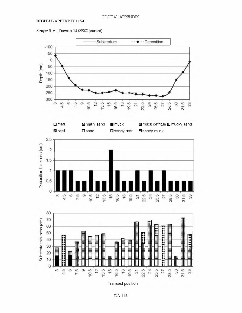
Subs

trate

th

ickn

ess

(cm

) De

posi

tion

thic

knes

s (c

m)

Dept

h (c

m)

DIGITAL APPENDIXDIGIT AL APPENDIX 115A

Strayer Run - Transect 14.09902 (curved)

h- co CO CJ)CN CN

COCN

CO COCO

□ marl □ m arly sand ■ m uck E3 m uck detritus EB m ucky sand

U p e a t □ sand □ sand y marl H s a n d y m uck

Transect position

DA-118

Subs

trate

th

ickn

ess

(cm

) De

posi

tion

thic

knes

s (c

m)

Dept

h (c

m)

DIGITAL APPENDIX

Strayer Run - Transect 14.09903 (straight)

DIGITAL APPENDIX 116A

□ marl □ m arly sand ■ m uck S m uck detritus El m ucky sand

□ peat □ sand □ sand y marl H s a n d y m uck

30

25

20

15

10

5 -

S

CO CD O) CN LO 00CN

^rCN

h-CM

OCO

COCO

CDco

jn u R R

•4 n►►►►

\FIMM

a i l ;<

H:

;HnnM

50

40

30

20

10

0 I “CO CD CD

nCN LO CO

CN CNh-CN

OCO

COCO

CDCO

Transect position

DA-119

DIGITAL APPENDIXDIGIT AL APPENDIX 117A

Strayer Run - Transect 14.09904 (straight)

^ K d c d c b a > c \ i L d c o T - ^ h -t— t— C N C N C N C O C O C O

□ marl □ m arly sand ■ m uck E3 m uck detritus El m ucky sand□ peat □ sand 0 sand y marl a sand y m uck

co CD CJ) CNCN

LOCN

COCN CO

rCO

h-co

(/)(/)CDco

313~co- Q=3

CO

L O L O L O L O L O L O L O L O L O L O L O L O^ r h - d c d c D d c N L d c o ^ - ^ r K

x— t— C N C N C N C O C O C O

Transect position

DA-120

Subs

trate

th

ickn

ess

(cm

) De

posi

tion

thic

knes

s (c

m)

Dept

h (c

m)

DIGITAL APPENDIXDIGITAL APPENDIX 118A

Strayer Run - Transect 14.09905 (straight)

c m c m c m co co co co

□ marl □ m arly sand ■ m uck 5 m uck detritus □ m ucky sand

@ peat □ sand □ sand y marl Q s a n d y m uck

CM c m c m co co co co

CM CM CM CO CO CO CO

Transect position

DA-121

Subs

trate

th

ickn

ess

(cm

) De

posi

tion

thic

knes

s (c

m)

Dept

h (c

m)

DIGITAL APPENDIXDIGITAL APPENDIX 119A

Strayer Run - Transect 14.09906 (curved)

CN CN CN CO CO

□ marl □ m arly sand ■ m uck 5 m uck detritus □ m ucky sand

@ peat □ sand □ sand y marl Q s a n d y m uck

4540353025201510

50

LO LO LO LO LO LO LO LO LO LO LO■vT d CO CD O') cn LO CO T—

T T T— CNI CNJ CN CO CO

70

60

50

40

30

20

10

0LO LO LO LO LO LO LO LO LO LO LO

o CO CD O) c n LO cd T—T— T CNJ CNJ CN CO CO

Transect position

DA-122

Subs

trate

th

ickn

ess

(cm

) De

posi

tion

thic

knes

s (c

m)

Dept

h (c

m)

DIGITAL APPENDIXDIGITAL APPENDIX 120A

UBX Run - Transect 19.1 (straight)

■Substratum ■ D eposition

LO LO LO lO LO LO LO LO LO LO LO LO LO LO LOT— T— ^r N- o CO CD CD CN LO CO T— h-

T T CN CN CN CO co co

□ marl □ m arly sand ■ m uck B m uck detritus Q m ucky sand

U p e a t □ sand □ sand y marl □ sand y m uck

60 -i

50

40

30

20

a a sa J J

yyyyyyyyyyyyyyyyyyyyy

LO LO LO LO LO LO LO LO LO LO LO LO LO LO LOT — T— o c d CD CD CN LO CO T — "ST h-

i i t — T — T — CN CN CN CO CO CO

50

40

30

20

10

0 n I n I I ~ I I I I I iLO LO LO LO LO LO LO LO LO LO LO LO LO LO LO

T— T— o cd CD CD CN LO cd T— 'vT h-i i t— T- CN CN CN CO CO CO

Transect position

DA-123

Subs

trate

th

ickn

ess

(cm

) De

posi

tion

thic

knes

s (c

m)

Dept

h (c

m)

DIGITAL APPENDIXDIGIT AL APPENDIX 121A

UBX Run - Transect 19.2 (straight)

CN CM CN CO CO CO CO

□ marl □ m arly sand ■ m uck S m uck detritus 0 m ucky sandU p e a t □ sand □ sand y marl H s a n d y m uck

60 n

CD CN LO COCNJ

^rCN CNJoco coco coco CD

CO

Transect position

DA-124

Subs

trate

th

ickn

ess

(cm

) De

posi

tion

thic

knes

s (c

m)

Dept

h (c

m)

DIGITAL APPENDIXDIGITAL APPENDIX 122A

UBX Run - Transect 19.3 (straight)

CN CN CN CO CO CO CO

□ marl □ m arly sand B m u c k S m uck detritus El m ucky sand

H p e a t D s a n d Q s a n d y m a r l a sand y m uck

o c o c o c d c n l o c o t - ^ i- ^ o c o c o o )t- t- \ - ( N C N C N C O C O C O C O

DA-125

Subs

trate

th

ickn

ess

(cm

) De

posi

tion

thic

knes

s (c

m)

Dept

h (c

m)

DIGITAL APPENDIXDIGITAL APPENDIX 123A

UBX Run - Transect 19.4 (curved)

CN CN CN co co

□ marl □ m arly sand ■ m uck B m uck detritus Q m ucky sand□ peat □ sand □ sand y marl □ sand y m uck

14 12 10

CO CD G) CN LO CO t-CN CN

h-CN

O COCO CO

CN CN CN CO CO

Transect position

DA-126

Subs

trate

th

ickn

ess

(cm

) De

posi

tion

thic

knes

s (c

m)

Dept

h (c

m)

DIGITAL APPENDIXDIGITAL APPENDIX 124A

UBX Run - Transect 19.5 (curved)

CN CN CM CO CO CO

□ m arl □ m arly san d H m u c k H m uck detritus O m ucky sand□ p eat D s a n d □ sandy m arl Cl sand y m uck

O C O C D C D C N L D C O ’i - ' s r r ^ O C O C Dt— C N C N C M C O C O C O

c o c o c D C N i n c o T - ^ r r - ' - o c o c ot— C N C N C N C O C O C O

Transect position

DA-127