SU-SEL-70-066

00

9

Aperture Synthesis for HF Radio Signals Propagated via the F Layer of the Ionosphere

by

J.T. Lynch

September 1970

Technical Report N0 161

This document has been approved for

public release and sale; its distribution is unlimited.

Prepared under Office of Naval Research Contract 1^0^-225(64). NR 088-019, and Advanced Research Projects Agency ARPA Order N» 196

RflDIOSIIElUE UUOIMTORV

STRHFORD EIEITRORIIS IHRORRTORIES STRnFORO UDIUERSITV • STRniORD, IRlirORRIR

Reproduced by NATIONAL TECHNICAL INFORMATION SERVICE

Springfield, Va 22151

DISCLAIMER NOTICE

THIS DOCUMENT IS THE BEST

QUALITY AVAILABLE.

COPY FURNISHED CONTAINED

A SIGNIFICANT NUMBER OF

PAGES WHICH DO NOT

REPRODUCE LEGIBLY .

. t. ; . ~·...,

SU-SEL-70-066

APERTURE SYNTHESIS FOR HF RADIO SIGNALS PROPAGATED VIA THE F LAYER OF THE IONOSPHERE

by

J. T. Lynch

September 1970

This document has been approved for public release and sale; Its distribution is unlimited.

Technical Report No. 161

Prepared Under

Office of Naval Research Contract ^onr-225(6U), NR 088-019, and

Advanced Research Projects Agency ARPA Order No. 196

Radioscience Laboratory Stanford Electronics Laboratories

Stanford University Stanford, California

rz mmr^m.-m. mm. tptMtl».

BLANK PAGE :

:

r^

;,

-ir- .■■"-, iai- 4<

•, ~

ABSTRACT

A portable high-frequency (HF) radio aperture up to 70 km in length

was synthesized by receiving ionospherically propagated signals in a

DC-3 airplane. By thus moving a small antenna rapidly over a long

distance, a narrow receiving beam width (high azimuthal resolution) was

achieved. It is believed that the synthetic aperture described here is

the first in the world developed for HF, although the concept has been

used successfully at microwave frequencies.

When HF radio signals are propagated by refraction from the

ionosphere, inhomogene ities in the electron density of the medium

distort the refracted signals and limit the azimuthal resolution which

can be achieved. Using a statistical model of the ionospheric distor-

tion a theoretical analysis was made to predict the performance of the

HF synthetic aperture, determine its limitations and compare its

performance with that of a ground-based fixed array.

Using continuous wave (CW) signals transmitted from a point 2600 km

to the east, it was shown that with compensation for the deviations of

the aivplane from a straight line course, a 10 km aperture yielded a

1/12 deg beam width (at 23 MHz) for about 20 per cent of the data

tested, while a 5 km apevture yielded a 1/6 deg beam for about 50 per

cent of the data tested. Based on results obtained by receiving the

same signal at a fixed antenna on the ground, it is believed that both

spatial and temporal variations of the ionosphere were limiting the

achievable beam width. In another method of operation a sequence of

swept frequency CW (SFCW) signals was transmitted from California,

backseattered from ground areas 2600 km to the east, and received in

the airplane, thus yielding an HF reflectivity image of the area. An

HF repeater was located near the terrain to be imaged and was used as a

reference to compensate for flight-path deviations and ionospheric

distortion. A second repeater located 1000 m away from the reference

repeater was used to simulate a strong backscatter return. An HF back-

scatter map was made using a 70 km synthetic aperture which had a 500 m

range and a 500 m cross-range (lateral) resolution. The two repeaters

iii SEL-"ü-066

were distinguishable in cross range. On the basis of the theoretical

analysis, and the characteristics of the two repeaters as revealed in

the backscatter map, it is believed that objects should be within 3 to

5 km of the reference repeater in order to be imaged without significant

distortion.

The above results were obtained on a midlatitude east-west path

which is known to have favorable characteristics. The data were taken

during a period of low magnetic activity and in general the ionosphere

was undisturbed.

It is concluded that aperture-synthesis techniques at HF are

particularly attractive for apertures of between 1 and 10 km in length.

For the shorter apertures, 1 to 3 km, it should be possible to obtain

full benefit of the aperture by using a medium-sized airplane and

simple processing techniques which would not compensate for course

deviations of the plane from a straight line. Longer apertures,

6 to 10 km, could be used effectively at least part of the time, if

compensation for course variations could be provided.

SEL-70-066 iv

CONTENTS

Page

I. INTRODUCTION 1

A. Purpose and Motivation 1

B. Previous Work in the Field . . 2

C. Approach Used in Present Study 6

D. Contributions of this Research 8

II. ANALYSIS OF AN HF SYNTHETIC APERTURE 11

A. Basic Relationships 11

B. Effect of Ionospheric Irregularities on a Fixed HF Array 15

1. Wave-Front Distortion Model an'i Mean Power Pattern of Array 17

2. Calculation of the Mean Array Power Pattern for Case of Short-Tertn Averaging 19

3. Interpretation of Calculations 28 4. Evaluation for Large Rms Phase Variance 34

C. Effect of Ionospheric Irregularities on a Synthetic Aperture 35

III. APPLICATION OF SIGNAL RESTORATION TECHNIQUES TO HF ARRAYS . 39

A. Use of the Optimum Filter in Overcoming Signal Distortion 39

B. Evaluation of the Optimal Filter for Two Special Cases 42

1. Effect of Noise in the Measurement of the Distortion 43

2. Effect of Changes in Multipath 44

C. Application of Signal Restoration Technique to HF Backscatter Sounding 46

D. Calculation of the Performance of an HF Aperture Which Uses a Phase Reference for Signal Restoration 49

1. Case of a Fixed Array 49 2. Case of a Synthetic Aperture 56 3. Evaluation of the Analytical Results for Typical

Ionospheric Parameters 58

IV. DESIGN OF THE HF SYNTHETIC-APERTURE EXPERIMENT 61

A. Basic Components of the Experimental System 61

SEL-70-066

CONTENTS (Cont)

VI.

B. Princinfl Features of the Experimental Prcgram .... 63

C. Systeu; Design 63

D. System Parameters 67

1. Backscatter Experiment 67 2. Forward-Propagation Experiment 71

E. Flight-Path Accuracy and Measurement 71

F. Digital Signal Processing 73

RESULTS 75

A. Verification of Airplane Tracking Subsystem Performance 75

B. CW Forward-Propagation Measurements 79

C. Backscatter Measurements Madt Without Compensation for Flight-Path Deviations or Ionospheric Variations ... 87

D. Backscatter Measurements Made Using Fixed Repeater Signal To Compensate for Airplane and Ionospheric Variations 90

1. Use of a Portable Repeater with Low Gain Antenna. 92 2. Use of Portable Repeater with High Gain Antenna . 94 3. Backscatter Data Taken with 12 km Synthetic

Aperture 96 4. Backscatter Data Taken with 70 km Synthetic

Aperture 99 5. Discussion of Delay and Cross Range Side Lobes. . 101

CONCLUSION Ill

A. Summary of Results Ill

1. Analytical Results Ill 2. Experimental Results 113

a. Airplane Tracking 113 b. CW Forward-Propagation Measurements 114 c. Backscatter Measurements Made Without

Compensation for Flight-Path Deviations or Ionospheric Variations 114

d. Backscatter Measurements Using a Repeater Signal to Compensate for Flight-Path Deviations and Ionospheric Variations, . . . 115

B. Conclusions 115

1. No Compensation 116

SEL-70-066 VI

CONTENTS (Cont)

2. Flight-Path Compensation 116 3. Flight-Path and Ionospheric Compensation 117 4. Overall Conclusions 117

C. Recommendations for Future Work 119

1. Other Forms of Compensation 119 2. Use of Faster and More Stable Airplanes 120 3. Use of Optical Processing vs Airborne Computer

Processing 120 4. Use of Longer Synthetic Apertures, Wider Band

Widths, Higher Frequencies, and Shorter Ranges, . 121 5. Use of Incoherent Processing Techniques 121 6. Use of Other Ionospheric Modes and Conditions . . 122 7. Applications to Direction Finding (DF) 123

Appendix A. DESCRIPTION OF EQUIPMENT COMPONENTS 125

Appendix B. DESCRIPTION OF SIGNAL PROCESSING 143

REFERENCES 157

vtl SEL-70-066

ILLUSTRATIONS

Figure Page

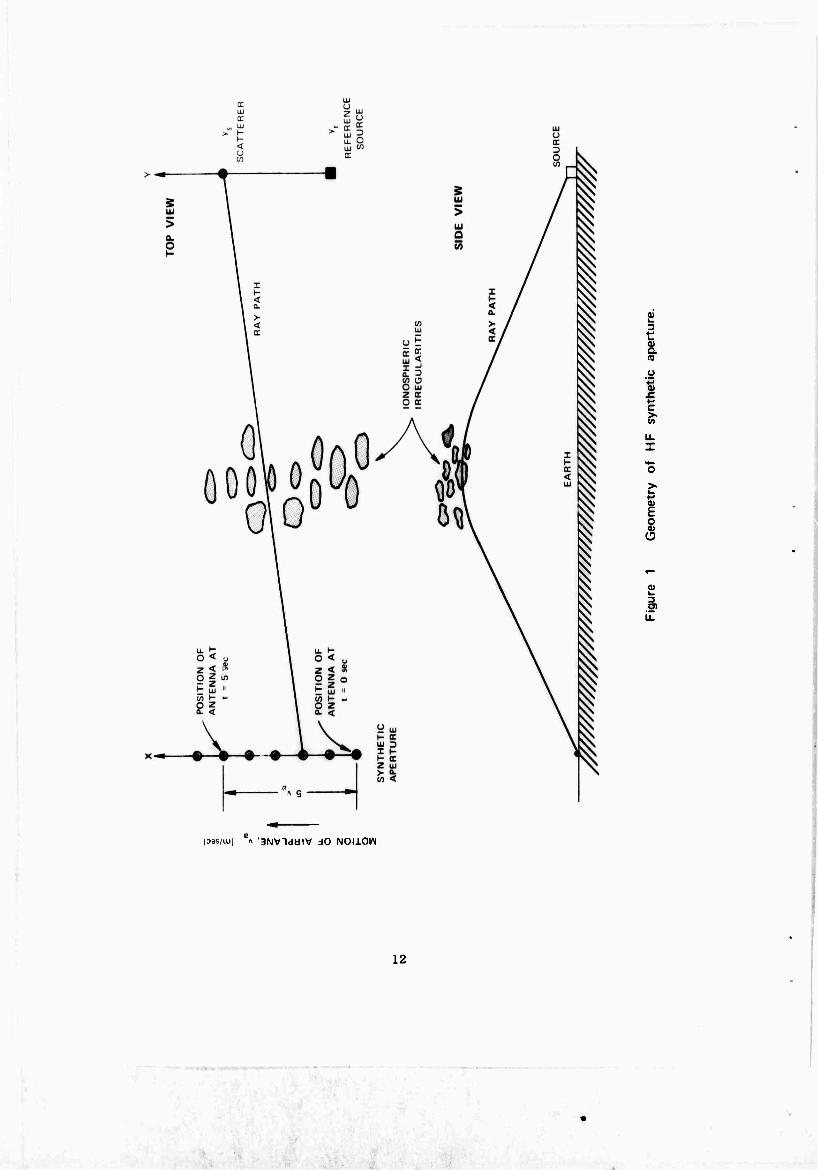
1 Geometry of HF synthetic aperture 12

2 Wave front after undergoing distortion 16

3 Sketch showing limits of integration In evaluating h (Ax). 25 ST

4 Normalized phase structure function 30

5 Normalized phase structure function 30

6 Normalized nonlinear phase structure function 31

7 Long-term distortion function 31

8 Short-term distortion function 33

9 Short-term distortion function 33

10 Use of the optimum filter in overcoming signal distortion. . '41

11 Amplitude of optimum filter transfer function jH (f)| ... 47

12 Rays crossing among ionospheric irregularities 53

13 Map indicating locations of transmitter, repeaters, and synthetic-aperture flight path 62

14 Detail map showing flight path in relation to Los Banos and to location of CW tracking transmitters 64

15 Diagram of signals for synthetic-aperture experiment .... 66

16 Deviations of flight path from straight line that represents mean-square best fit for position data taken over entire flight path 76

17 Rms deviations of flight path from a series of straight lines representing mean-square best fits, for position data taken over various segments of flight path 77

18 Frequency spectrum of forward-propagated CW signal received at Los Banos--64 sec processing time 79

19 Frequency spectrum of forward-propagated CW signal received at Los Banos--128 sec processing time 80

SEL-70-066 viil

ILLUSTRATIONS (Cont)

Figure Page

20 Frequency spectrum of forward-propagated CW signal received at Los Banos--256 sec processing time 81

21 Angular spectrum of forward-propagated CW signal received In alrplane--6A sec processing time, equivalent to 6 km aperture 84

22 Angular spectrum of forward-propagated CW signal received In alrplane--128 sec processing time, equivalent to 12 km aperture , 85

23 Backscatter map: Normalized amplitude vs delay and azimuth. 88

24 lonogram, Bearden to Los Banos, 22 April 1969, 22:34 GMT . . 89

25 Backscatter map of normalized squared amplitude vs delay and azimuth, showing enhancement at 1600 km 91

26 Sketch showing two locations at which portable repeater operated 93

27 Normalized amplitude vs relative delay for a sequence of equivalent elements of the synthetic aperture (Flight 3N on 26 April 1969) 95

28 Normalized amplitude vs relative delay for sequence of equivalent elements of the synthetic aperture (Flight 3N on 22 April 1969) 97

29 lonogram, Bearden to Los Banos, 26 April 1969, 22:45 GMT . . 98

30 Backscatter map of normalized squared amplitude vs delay and cross range for flight 3N on 22 April 1969 (same flight as Fig. 28) using 12 km synthetic aperture 100

31 Backscatter map of normalized squared amplitude vs delay and cross range, using same data as Fig. 30 but with a 70 km synthetic aperture 102

32 Backscatter map made with 70 km synthetic aperture, using same data as In Fig. 31, but using compensation for amplitude and phase distortion caused by Ionosphere and by flight-path deviations 104

ix SEL-70-066

t[.l."S TRAT IONS (Com)

Figure Page

JJ Airplane used In synthutic aperture experiment, showing horizontal ami vertical tuhular antennas 128

i't S imp 1 it Led block diagram ol receiving equipment 130

J3 Detailed block diagram ot" receiving equipment 131

Jd Geometry Cor spherical wave£ront calculation 150

J7 Flow chart lor beamforming program 155

SBL-70-066

TABLES

Number Page

1 Parameters of backscatter experiment 69

2 Summary of experiment log 109

3 Summary of geomagnetic activity Index (K ) 110

4 Tape recorder channels 135

xl SEL-70-066

ACKNOWLEDGMENT

I wish to express special thanks to Professors 0. G. Villard, Jr.

and J. W. Goodman for their guidance and encouragement throughout this

work. I am also grateful to Professors L. A. Manning and M. A. Arbib

for their suggestions for improving the manuscript. My thanks also go

to Mrs. Mabel Rockwell for editing, and to Miss Jane King and Mrs. Carol

Cook for typing, the finished report.

I gratefully acknowledge the help of the personnel from Western

Aerial Photos, Inc. who obtained, outfitted and flew the airplane; the

Stockton FAA office who allowed us to use their facility on Bear

Mountain; and the Rosemont Engineering Company who donated a precision

barometric altimeter. I owe special appreciation to Dr. P. A. Fialer,

who shared in the responsibility of running the experiments, since he

conducted his doctoral research on ionospheric irregularities and used

the same ground-based and airborne equipment as was employed in the

present study. Dr. Fialer developed the airplane tracking sub-system

and did most of the data reduction for the CW signals in the forward-

propagation experiment. The members in the Ionospheric Dynamics Group

of the Stanford Electronics Laboratories contributed many long days in

helping to prepare experimental equipment and computer programs for the

project. Their effort is greatly appreciated.

The work was funded by the Advanced Research Projects Agency, with

the Office of Naval Research, under contract Nonr-225(64). The author

appreciates this support.

SEL-70-066 xli

I. INTRODUCTION

A. PURPOSE AND MOTIVATION

The purpose of this research was to explore the possibilities of

synthesizing an extremely long, high-frequency (HF) radio receiving

array. This synthetic aperture is used to obtain the narrow beam width

(high azimuthal resolution) possible with a large aperture by moving a

small antenna rapidly over a large distance. This was accomplished by

flying HF receiving equipment in an airplane over a path which formed

the center line of the synthetic array. A sequence of pulsed signals

propagated a long distance by means of an ionospheric reflection was

received by the plane in flight. The information received at each

position along the flight path was essentially equivalent to a signal

received by a hypothetical dipole of a fixed array at that position.

By receiving data in this manner in a plane traveling about 180 mph for

up to 20 minutes it should be possible to synthesize arrays up to 100 km

in length.

The investigation was undertaken because previous work In the

Ionospheric propagation of HF signals had shown that at least under

favorable Ionospheric conditions, the spread In azimuthal angle of

arrival caused by irregularities In the Ionosphere was often smaller

than could be detected by arrays of the sizes used In the measurements.

Some of these measurements have been made on what Is believed to be the

longest ground HF array now available, a 2.5 km phased array operated

by the Stanford Radlosclence Laboratory at Los Banos, California. It

was hoped that the synthetic aperture technique would demonstrate that

apertures much longer than 2.5 km could be used at HF to form very

narrow beam widths. The synthetic-aperture concept Is very attractive

at HF because of the large size of the physical structures otherwise

required to obtain very narrow beam widths. The cost and time of laying

cables for even a 10 km array are prohibitively large. The synthetlc- 2

aperture technique has proven successful at microwave frequencies;

however, the use of this technique at HF poses many new problems because

•

of the much longer wave lei ^ths and therefore the much longer arrays

which are required to obtain narrow azimuthal beams, and also because

of the inhomogeneous nature of the ionosphere, which has a pronounced

effect at HF.

There appear to be many potential applications for HF synthetic

apertures, such as obtaining more detailed backscatter images of the HF

reflectivity of the ground. It has been known for decades that HF radio

signals can be propagated via the ionosphere to distant regions of the

earth, scattered, and reflected back to a receiver near the source. For

even the best existing HF backscatter sounding systems, the cross-range

(measured perpendicular to signal path and is proportional to the angle

of arrival times the range) resolution (10,000 m at a range of 2600 km),

or detail obtained in this "backscatter" process is about two orders of

magnitude less than the range resolution (measured parallel to signal

path and is proportional to signal delay) (300 m). The backscatter

records therefore contain only spatially averaged information about the

ground scattering characteristics.

Using a 100 km aperture, a cross-range resolution of about 500 m

at a range of 2600 km could theoretically be possible. With a cross-

range resolution and a range resolution of about 500 m each, it might

be possible to identify individual scatterers on the ground.

This research should also have implications regarding the ability

of fixed arrays on the ground to obtain much narrower beam widths than

previously demonstrated. There may be applications for which the cost

and complexity of a large fixed array would be warranted if some

assurance could be given that it would produce very narrow beam widths.

B. PREVIOUS WORK IN THE FIELD

Synthetic-aperture radars have been successfully used at microwave 2 3

frequencies for many years. ' These radars often operate at wave

lengths of a few centimeters and at a line-of-sight distance from the

terrain they image. They produce optical-quality radar reflectivity

maps at least as us:ful as optical photographs. 4

A synthetic aperture for HF has been proposed by Shearman, who

- ,'.v- i,.i:-.,.,r ,

•

described an incoherent processing technique similar to the radio-

astronomy approach. The incoherent HF technique takes advantage of the

temporal variations of the ionosphere, requires a long averaging time,

and depends on the randomness of the phase fluctuations. It is not

obvious, however, that the statistics of the phase fluctuatioiis of

ionospherically propagated signals have the nficessary properties in

order for the incoherent approach to work. Therefoje. the technique

and implementation described here are based on coherent processing just

as is the microwave technique. The coherent processing approach is

used in this study because, as is later described, the ionosphere

appears to preserve signal coherence over distances on the order of

2-10 km. Ic was also desired that the results apply directly to

conventional large arrays which use coherent processing.

Many solutions to problems of the microwave synthetic aperture are

directly translatable to the HF implementation. A problem not encoun-

tered at microwave frequencies, however, is the distortion caused by

inhomogeneities in the propagating redia. The ionospheric distortion

may not limit the performance of arrays of about 2 to 10 km in length;

however, the induced signal incoherence may be severe for arrays longer

than 10 or 20 km. To determine the effect of the inhomogeneities on

the performance of an HF array it is necessary to know the spatial and

temporal statistics of the amplitude and phase distortion of obliquely

propagated HF signals. While much is known about such ionospheric

inhomogeneities, as is described below, there are many unanswered

questions which the synthetic aperture experiment might help answer.

The ionosphere is composed of free ions, electrons and neutral

particles as a result of solar radiation interaction with the earth's

atmosphere. The electrons exert the major influence on HF radio signals

by decreasing the refractive index thus causing radio rays from the

earth to bend and return to earth. Although the process is often a

gradual bending of the ray the term reflection is used to emphasize the

major effect. The maximum electron density is near 300 km (which varies

diurnally and seasonally) and drops off nearly monotonically to approxi-

mately zero both near the earth and in interplanetary space. The

Signals used in this study were reflected by the F layer, which Is the

region of the ionosphere near the electron density maximum. At a lower

height there is sometimes a local maximum of electron density or some-

times just a variation in the rate of change with height of the electron

density which is called the E-layer. Propagation using the E-layer can

have more stable characteristics than F-layer propagation. It can be

used, however, only for distances shorter than those used in this study.

All signals used in this study were propagated via a single ionospheric

reflection, i.e., one hop. Two and three hop signals are common; how-

ever the intervening ground reflection can greatly distort the signal.

The electron density in the ionosphere is spatially inhomogeneous

as a result of many different mechanisms such as temperature fluctua-

tions, solar radiation changes, interaction of the plasma with neutral

winds and wave motions and the passage of meteors. Traveling iono-

spheric disturbances with spatial periods of 50 to 500 km are often 5

observed (see Georges for a review). Satellite-to-ground radio

measurements indicate regions of the irregularities near or above the

F-region peak. Size estimates for these irregularities are on the

order of 1 km. However, the nature of the irregularities below the

F-region peak is of most interest here, since obliquely propagated HF

signals are always below this level.

Vertical incidence measurements and incoherent scatter observations 8 9

of traveling disturbances have also been made (see Thome ' ) with a

sensitivity of about 1 per cent of the ambient electron density.

The techniques mentioned above do not appear to be sensitive to the

presence of weak irregularities which apperr to exist even under quiet

conditions. To avoid confusion in interpreting results, it would be

best to make observations of the irregularities with obliquely propa-

gated HF signals if the effect of the irregularities on this type of

signal is to be determined.

The oblique measurements should be made using a signal propagated

by only a one hop path. The intervening ground reflection of the

multi-hop case and the interference between the several modes apparently

explains why most of the research so far conducted shows a low degree of

spatial and temporal coherence. There have been a few experiments

reported which use a single mode and significantly conclude that the

wave coherence is very good.

In a 1951 paper entitled "Measurements of the Direction of Arrival

of Short Radio Waves Reflected at the Ionosphere," Bratnley and Ross

report that direction-of-a:rival measurements, made at two sites

laterally separated by 2~ km, were highly correlated. This suggests

that large inhomogeneities in the ionosphere are responsible for the

angle-of-arrival fluctuations. Bratnley and Ross indicate that there

may also exist smaller, weaker, irregularities which could affect the

phase of HF signals. A 1953 paper by Bratnley is similar to the

earlier one but investigates more fully the nature of large-scale

irregularities and their effect on angle-of-arrival measurements. The

characteristics of the large disturbances are of considerable interest

in HF direction finding. A paper reviewing this subject has been 12

written by Getning.

Recent measurements made at Stanford University provided basic

information and were a motivating factor for the research described

here. These measurements indicated that one-hop signals can be more

phase coherent thar previously thought. Delay-resolution measurements 13

of one-hop F-layer signals by Lynch e^ a^l show that 1 to 5 p,sec pulses

can be propagated without significant spreading, at least during favor-

able conditions. These conditions include a midlatitude path, propa-

gating in winter atfmidday, using a one-hop F lower ray mode and an

operating frequency iabout 70 per cent of the maximum usable frequency

(MUF). Coherent band widths of 500 kHz are possible at least part of

the time under these conditions.

Angular resolution measurements have been made by Sweeney using

HF antenna elements which span 2.5 km. Mode-resolved amplitude and

phase measurements made at eight elements of this a y indicate that

the wave fronts are nearly linear for the ideal propagation conditions

described above. This implies that beam widths at least as good as

1/4 deg at 30 MHz are possible at least part of the time over a favor- 14

able path. In a recent paper, Fialer indicates that there are weak

(1 per cent or less) slow-moving Irregularities with a typical size of

about 35 km.

Mode-resolved measurements made by other researchers also indicate

a high degree of coherence for one-hop F-layer signals. A paper written

by Baiser and Smith in 1962 reports on amplitude measurements made on

a 1500 km path with a lateral separation between receiving antennas of

up to 700 m. Baiser and Smith assume that the amplitude variations were

caused by scattering from many inhomogeneities in the ionosphere, and

they are able to relate the amplitude correlations to the angular spread

of the scattered signals. They estimate that the spreading was about

0.2 deg in azimuth, much less than predicted in earlier research. Re-

gardless of the validity of their assumptions and conclusions of the

analysis, their experimental results, indicating a high degree of

spatial amplitude correlation in ionospherically propagated signals,

are significant. Measurements of temporal variations have been made;

however, only a few of these measure the frequency spread introduced by 1 6

the ionosphere. Sheperd and Lomax report frequency spreads of less

than 1/10 Hz for one-hop F or E modes.

Mode-resolved measurements of phase difference of obliquely

propagated signals at points separated by more than 3 km have apparently

not been made. Thus the upper limit on how far HF arrays can be ex-

tended and still achieve the beam widths predicted from theory has not

been determined. The synthetic-aperture technique offers the possi-

bility of determining a lower bound on the performance of large arrays.

Such a bound is determined because the temporal variations of the iono-

sphere degrade the performance of the synthetic aperture but do not

affect the fixed aperture.

C. APPROACH USED IN PRESENT STUDY

The approach used in this investigation is to show the feasibllty

and determine the fundamental limitations of HF synthetic apertures by

using a simple but realistic analysis and experimental measurements de-

signed to use existing equipment and techniques whenever possible.

Three possible methods of operation have been developed for the

synthetic aperture. These methods are;

1. Operation without compensation for airplane flight path deviations from a straight line or for ionospheric distortion.

2. Operation with compensation for flight path deviations by means of an airplane tracking system, but without compensation for ionospheric distortion.

3. Operation with an HF repeater used to provide a reference signal to compensate for both flight-path deviations and ionospheric distortion.

The first method, in which no compensation is used, is by far the

simplest in terms of signal processing and is attractive for this reason.

The second method, in which compensation for airplane course

deviations is made, requires some technique to accurately determine the

coordinates of the plane as a function of time. Thus the measurements

will indicate the limitations imposed by the ionosphere on a synthetic

aperture.

The third method, in which compensation for airplane course

deviations and ionospheric distortion is made, offers the possibility

of obtaining extremely long synthetic apertures. The use of an HF

repeater to measure the distortion is similar to the use of a reference

beam in optical holography to reduce image distortion. It has been

shown by Goodman that holograms are superior to conventional incoher-

ent images if the medium through which the light passes is turbulent.

If the object and the reference beam are close enough to each other,

the random phase variations in the optical signal are cancelled because

the reference beam for the hologram and the light .from the object pass

through nearly the same random variations in refractive index.

The principal features of the experimental program are:

1. Verification of airplane tracking subsystem performance.

2. Measurement of beam width achievable with synthetic aperture when receiving a CW signal transmitted from Bearden, Arkansas (CW forward-propagation experiment). In this test, compensation was made for deviations of the

7

■

airplane from a linear flight path by the use of the airplane tracking data.

3. Demonstration of feasibility of obtaining two- dimensional backscatter data (range vs cross range) without compensating for ionospheric distortion or deviations of the airplane from a linear flight path,

4, Investigation of the use of an HF repeater at Bearden to provide a reference signal in compensating for airplane flight path deviations and ionospheric distortion, for the purpose of obtaining extremely high azimuthal resolution in backscatter mapping.

The CW forward propagation experiment has the advantage of much

simpler signal processing requirements, thus making it easier and less

expensive to process more data. The backscatter experiments are Im-

portant, however, to illustrate application of synthetic apertures to

HF backscatter Imaging. The use of both approaches also makes it

easier to compare the results obtained with both forward propagation

and backscatter studies being performed by the Stanford Radioscience

Laboratory with the 2.5 km array at Los Banos.

As indicated earlier, the experimental design was to use existing

facilities and equipment whenever possible. Thus the Stanford Radio-

science Laboratory's existing wide-band, high-power, narrow-beam

transmitter at Lost Hills, California, the transmitter and repeater at

Bearden, Arkansas, and the swept frequency CW (SFCW) sounding equipment

were all part of the design. The digital computer processing is avail-

able at Stanford and allows considerable flexibility in specifying and

changing the signal processing. It is expensive to use a large computer

such as the IBM 360; but as only a few backscatter images were to be

made, this was cheaper than other approaches. The use of a digital

computer also makes it possible to implement more complex signal

processing techniques.

D. CONTRIBUTIONS OF THIS RESEARCH

During the course of this research the following original

contributions were made in the field of ionospheric propagation of HF

radio signals;

8

1. A portable HF radio antenna aperture of up to 70 km In length was synthesized by installing receiving equipment aboard an airplane which flew a substantially straight course while receiving ionospherically propagated signals. It is believed that this long synthetic aperture is the first in the world to be developed for operation at HF.

2. A theoretical analysis was made to predict the performance of such a synthetic aperture, determine its limitations and compare its perfon anee with that of a ground-based fixed antenna array.

3. The problem of restoring signals to their undistorted form was studied for application to HF synthetic apertures. The improvement afforded by a reference signal was calculated in order to predict how far a point to be imaged could be from the reference and still have a small degree of distortion.

4. Using such compensation techniques it was shown experimentally that a very high degree of azimuthal resolution can be obtained within 3 to 3 km of an HF repeater used as a reference signal. An HF backscatter map using a 70 km aperture was made showing a second repeater used to simulate ground backscatter.

5. It was also shown experimentally that synthetic apertures 6 to 10 km in length can be ustd effectively at least part of the time (i.e., under favorable ionospheric conditions) if compensation for only flight path deviations are made.

f i — J- -l—H v

'

•<

BLANK PAGE

..

■«»

•• £— mmmmtmM^immmm

"

II. ANALYSIS OF AN HF SYNTHETIC APERTURE

A. BASIC RELATIONSHIPS

The use of a synthetic aperture for HF radio reception is a

technique for obtaining the narrow beam width (high azimuthal resolution)

possible with a large aperture by moving a small aperture rapidly over

a large distance. Consider a sequence of HF pulses from a distant fixed

source with a period of T sec. The pulses are identical, and each

pulse has a plane wave front. A small receiving antenna moves at a

uniform velocity of v m/sec, as shown in Fig. 1. The antenna, in 3

effect, samples each arriving pulse at uniformly spaced points along

the wave front. If N pulses are coherently processed, the result

should be equivalent to that obtained if signals were processed from N

fixed elements spaced Tf v meters apart along the flight path of the

airplane. The beam width of the synthetic aperture is equal to the wave

length \ divided by the total equivalent aperture length N T v , i 3

or \/N T, v radians beam width, r a

An equivalent point of view considers the frequency shift

("doppler") introduced by the motion of the receiving antenna. If N

pulses are coherently processed, the integration time is N Tf sec,

and the frequency (doppler) resolution is 1/N Tf Hz. This resolution

is a measure of how closely spaced in frequency two signals can be, and

yet be distinguished from each other. A distant source whose signal

arrives perpendicularly to the path of motion of the antenna has zero

doppler shift, A source 9 radians from the first has a doppler shift

f, given by

_a f , - -f sin 6

For small 6 , where sin 6 s= 6 , the angular resolution is the "doppler

resolution" (1/N Tr) times X/v , giving a resolution of X/(N T, v ) t 3 13

ii Preceding page blank

■

<u i.

(U Q. CO

0)

c >•

E o

3

{D3s/ui) A 'aNVldülV dO NOIiOW

12

radians. Thus the analysis gives the same conclusion regardless of the

point of view.

The first point of view—i.e., that of an equivalent array fixed

in space--will be taken to describe the performance of the synthetic

array. Although the synthetic array is actually composed of discrete

equivalent elements, it is convenient to describe its performance in

terms of continuous rather than discrete variables. It is assumed that

in practice the elements of the array are close enough together to avoid

a problem of multiple side lobes caused by spatial aliasing ("grating

lobes").

Let the received signal voltage at a point x along the array of

length L be represented by the real part of

s(x) = A(x) e jcp(x)

where A(x) = the amplitude of the received signal

cp(x) = the "phase"--i.e. , the phase difference between the incident wave and the local oscillator of the receiver.

Let S(0) be the complex angular distribution of signal amplitude 18

and phase; then (see Bracewell )

1/2

8(8) = i J s(x) exp(-j J -L/2

2 rrx sin 6 dx (1)

For small angles (sin 1*9), Eq. (1) becomes a Fourier transform

with the quantity 6A interpreted as a spatial frequency.

If the signal amplitude across an aperture of length L is unity,

and the phase Cp is linear according to the relation

13

■ , ?, ; ^ •.,-».-.-«•w«"-,"

cp(x) o u

where 9 is a constant expressed in radians, then the distribution of

received power vs angle (often called the "array power pattern") is

given by:

18(8) sin

TT(e - e ) L 2

rue - e ) L o

(2)

The resolution of the antenna is determined by its beam width and

side-lobe level. The beam width is often defined as the width of the

main lobe of the antenna at the half-power point (3 dB below the peak),

although a point 10 or 20 dB down is also often used. The 3 dB width

of the antenna pattern described by Eq. (2) is about X./L radians. The

largest side lobe is 13 dB below the peak. Techniques to reduce the 19 side-lobe level are well known, and one of the simplest will be used

here. The reduction is achieved by multiplying the data along the

aperture by a weighting function W(x) given by:

W(x) =

1 + cos 2 TT L . . L 2< x< ^

otherwise (3)

The effect of the weighting is to broaden the main lobe slightly and to

reduce the largest side lobe amplitude to approximately 30 dB below the

peak amplitude.

14

, -cf . .

B. EFFECT OF IONOSPHERIC IRREGULARITIES ON A FIXED HF ARRAY

The angular resolution of an antenna may be lost if the wave fronts

are no longer planar as was assumed in the initial model. Wave-front

distortion can be caused by irregularities in the medium through which

the signal passes. A statistical model of these wave-front distortions

is used to analyze their effect on the array. The array performance is

characterized by the statistical expectation (mean) of its power pattern.

The random wave-front distortion can be considered to be made up of

two components, a random tilt or change in the apparent direction of

arrival of a signal, and the variations about the tilt (see Fig. 2).

A changing random wave-front tilt displaces in azirauthal angle the

signals received by the array, but does not degrade the resolution by

widening the main lobe or increasing the side lobes _i_f the data are

collected, or time averaged, in a time interval short relative to the

time required for changes in the wave-front tilt. This case is referred

to here as the short-term average.case. In the long-term average case

the changing wave front tilt will smear the received signal in azimuthal

angle. The situation is analogous to photography with a moving camera.

The blurring caused by the camera motion can be reduced by making the

film exposure-time interval shorter. The analysis for the long-term

average therefore includes the effect of changing random wave-front

tilts, while the short-term average excludes them. Each equivalent

element of a synthetic aperture receives data essentially instantane-

ously; therefore the short-term average case also applies to synthetic

apertures regardless of the temporal variation of the propagation medium.

The distinction between long- and short-term has been made in the 20 21

context of optical imaging by Fried and Heidbreder. Their analyses

are more complicated and more difficult to interpret than that to be

presented here, because they used an accurate but awkward definition

of wave front tilt, and also because they characterized the wave front

variations with a statistical model which, though not necessarily more

accurate than the one used here, was far more difficult to treat

analytically.

15

■

DIRECTION OF SIGNAL

WAVEFRONT $ (x)

CENTER LINE OF ARRAY

TANGENT TO WAVEFRONT AT

POINT x TILT T (x) '

d ^ (x)

dx

Figure 2 Wavefront after undergoing distortion.

16

■

'

1. Wave-Front Distortion Model and Mean Power Pattern of Array

The electron density in the ionosphere is temporally changing

and spatially inhomogeneous as a result of many different mechanisms

such as temperature fluctuations, solar radiation changes, interaction

of the plasma with winds of neutral particles and wave motions, and the

passage of meteors. These changing ionospheric inhomogeneities cause

the wave-front distortion just discussed. These distortions are char-

acterized here by a phase distortion in the received signal. The phase

distortion is the phase difference between the phase which would have

been measured in the absence of ionospheric inhomogeneities and the

phase which is actually measured in the presence of the inhomogeneities.

For the purpose of the analysis it is assumed here that the phase distor-

tion cp , is a stationary gaussian, zero-mean rtndom process with a

correlation function given by

K (Ax) = ECcp(x) cp(x - Ax)]

(4)

2 = a exp cp •w

where Ax is the distance between two points at which the phase is 2

measured; a is the "phase variance"--i.e. , the mean square of the CD

phase cp ; A is the phase correlation distance; and £[•] denotes a

statistical expectation (here called the mean). This is clearly a very

simple model of a complicated phenomenon; however, it has several char-

acteristics required by the physical mechanisms involved. For example,

the phase variance is bounded, the correlation function is monotonically

decreasing, and the correlation function is differentiable (thus, the

phase process is uniformly continuous). A more complicated model could

be developed by using a correlation function which is the sum of several

functions similar to the above with different correlation distances A .

The simple function (4) should be useful, however, in relating the

17

. ■

correlation distance A to the performance of the antenna system. It

is to be noted that nonstationary variations, such as would be caused

by diurnal effects, are disregarded. The only cases considered here

are those in which amplitude distortion caused by focusing of the beam

by the ionospheric irregularities is small.

The phase-structure function is defined by

Dp (Ax) Ä E[|cp(x) - cp(x - Ax)|2] (5a)

It is related to the correlation function by

Dp (Ax) = 2[Kcp(0) - Kp(Ax)] ,

and for the assumed correlation function Eq. (4), the phase-structure

function is given by

DCp(Ax) = 2 a ?

exp nf] (5b)

A simple, already-known result will now be described which

relates the phase-structure function to the distorted power pattern of

an array. Since it includes the effect of random wave-front tilts the

following result is for the long-term average case.

Let h T(Ax) be a distortion function defined by

hLT(x) i exp [-^(Ax)] , (6)

18

and let HL (9) be given by

«LT^ h (Ax) exp [- j —^— Ax] dAx

where dAx is the differential of Ax . Then the mean array power 9 0 0

pattern, E[|s(e)| ] , is (see Gaskill )

E[|s(e)|2] = M j J 1" POO p(x - Ax) d>

• 2TT9 . - j —— Ax

hLT(Ax) e dAx

(7)

Equation 7 is a special case of a more general result which is derived

in the following section. This is a special case because D (Ax) does

not depend on x (only on Ax).

2. Calculation of the Mean Array Power Pattern for Case of Short-Term Averaging

The distortion function defined in (6) is appropriate to the

case of long-term averages because it includes the effect of random

wave-front tilts. The wave-front tilt, T(x) , is defined as the slope

of the phase of the signal at any point x (see Fig. 2). The angle of

arrival 6 , of a signal received at a point :.. = 0 , is related to

the tilt by 6 = T(0) T— . The tilt at a point x is given by

TW " dx 6x_*0 cp(x) - cp(x - 6x)

6x (8)

where 6x represents an incremental value of x (not to be confused

19

M*«^ SV « -^M > „ ' ' fi * Hfrs-TIP?

with Ax , the distance between two discrete points at which the phase 2

is measured). The variance of the tilt, a , is given by

2a2

E|T(x)|2 = -4- (9a) A2

2 and the variance of the angle of arrival Cg is therefore

o

2

öo (2nr ^ A

The short-term average distortion function is designated by

hST(x) , and is calculated with the linear phase-vs-dlstance part of

the phase distortion removed. Define Dm(^x) as the "nonlinear"

phase-stncture f unction--! .e., the function wiu. an approximation to

the linear phase term removed. An approximation to the short-term

average distortion function is then given by

hST(Ax) = exp [-ljDNLUx)]

The approach taken here is to approximate the exact result by

subtracting from the phase difference {cp(x) - {p(x - ^x)} a phase which

depends on the wave front tilt aX the center of the array (x ■ 0) .

This approach will yield a lower bound on the antenna performance, since

the actual amount of displacement of the array beam is given by the

average tilt across the entire aperture. Thus there may be some

20

residual tilt left in the calculations presented here which will cause

the distortion predicted to be greater than the actual distortion. 0 0 0

In the derivation of the expression for E[|s(9)| ] , Eq. 7,

it was assumed by Gaskill that the phase structure function D (Ax) ,

Eq. 5a, depends only on Ax but not on x . In the development to

follow it is found that D (Ax) depends on x as well as Ax and

therefore it is necessary to derive a new expression which is an upper

bound on the quantity E[|s(0)| ] . This bound is consistent with the

use of the wave front tilt measured at the midpoint of the array since

It too places an upper bound on the array performance, i.e., the actual

performance is better than the predicted performance.

Define an "aperture function" p(x) by

P(x) 2^ Xfi 2

otherwise

and let the received signal 8(x) be given by

s(x) = J^x) - (x) • T(0))

where a linear phase due to the wave front tilt has been subtracted and

where the amplitude is assumed to be unity. Using Eq. 1 the mean square

power pattern of the array is given by

21

■ ,

E 8(6)' = E

+ oo 1 L J

- 00

pCXj) sCx^ exp ( - j 2 TTX.eX

+ 00

i r L J

2 TTX e 2 p(x2)s*(x2) expl+ j ^— Jdx2

where t* (x7) denotes the complex conjugate of s(x„).

The previous equation can be rewritten by forming a double integral,

taking the expectation inside the integral and using the fact that (see 22

Gaskill" ) for a zero mean gaussian random variable a",

E[exp(± ja)] = exp[-i|E(« )]

Thus the expression for E[lS(9)l ] becomes

-f- 00

Er|s(S)|2] = "7 JJ Pi*^ P(x2) exp

Li - 00

^j<p(x1) - cp(x2)

(x1 - x2)T(0)|?] exp - J

2 TT(X - x2)e dx dx2

Let x - x„ = Ax and define a nonlinear phase structure function

DNl(Ax , Xj) by

D^C.x, x,) Ä ECl^CXj) - ca(x1 - Ax) - (Ax)T(0)| ]

22

The expression for EC|S(0)|2-| can be written as

+ 9»

ECls(e)n = ^ p(x1) p(x1 - Ax) exp [- ^D (Ax, x1 )]

exp^- j —j dxj dAx

Rearranging, it appears as;

+ »

E[|s(e)l2] = f + 00

i r L .

pix^ p(x1 - Ax) exp [- ^D (Ax, xj] d^ Nl/

exp / . 2 TTAXS \ ,

+ oo

L J ST (Ax) exp ( . 2 TTAXG

) dAx (10)

where h (^x) will be called the short term distortion function. The

distortion function h,, (Ax) is essentially an aperture weighting

function. If h__(Ax) becomes small for large Ax then there is a

restriction on the maximum size of the aperture which can be effectively

used and therefore there Is an expected beam width defined. By approxi-

mating hc_(Ax) with functions which are always smaller than hCT(Ax) l 2

an upper bound for E[|S(9)| ] can be found. That is the actual per-

formance will be better than that predicted by the calculation. The

first step Is to upper bound the Integral in the above equation which

depends on x^ . This Is done by noting that for positive ^x the

23

lüiuts of the Integral can be modified (see Fig. 3 for illustration on

integration limits) to account for the function piy^ ) as follows

-t- co

E [|s(e)|2] - i J p(Xl) p(xl - Ax) exp [- k DNL(Ax, ^)] dxl

L/2

I -(L/2-Ax)

exp [- ^Dj-^x, x1)]dxl , 0 < Ax < L

(U)

Ax > L

The symmetry in the definitions of DNL(Ax, xl) implies that the result

of the integration is even in Ax , thus it suffices to evaluate the

above for positive Ax .

The next step is to place an upper bound on the second integral.

This is done by noting that e l is a convex function, namely

h [e-zi + e"

23 ] 1 e- ^Zl + Za) .

It follows that, for 0 £ Ax < L,

L/2

L - Ax exp [ -b(z)] dz ^ exp

-a/2 - Ax)

L/2

"h^ J b(2)dz -(L/2 - Ax)

where b(z) is any integrable function. Using this Inequality and

Eq. 11, we can now write

24

- -^ ■"■■

FT- ) V* IJ^W .

p(x)

P(x)

V P(X-AX)

Region of overlap defines integration limits as -(L/2 + Axl. to L/2 for positive Ax

- 2

1

Wm. m m »

-L 12 -L/2 + Ax L/2 L/2 + Ax

Figure 3 Sketch showing limits of integration in evaluating hST(Ax).

25

.4.^ x *•"*'■''&&*- -*

L - Ax

■. .- -■.- ...^ .■:■:■,.-■.<::■■ .,■ ■ .

L/2

L - Ax J k DMT(Ax, X!) e ' NL dxi

•(L/2 - Ax)

> L - Ax 2 —■ exp < 2(L - Ax)

L/2

I ^^ Xl) dXl •(L/2 - Ax)

and the term in the exponential is written as

<DNL

(AX)> ■ r-TÄ^

L/2

I ■(L/2 - Ax)

DNL(^, xx) dXi

to indicate a spatial average over xi . Here hs_(Ax) Is a lower

bound on the actual distortion function h (Ax) defined in Eq. 10.

The function D.„ (Ax, x) is now evaluated and the integral per- NL

formed. Using the definition of tilt in Eq. 8 the correlation function

defined in Eq. 4, and the phase structure function in Eq. 5a D (Ax, x)

can be evaluated to be

DNL(Ax. x) D (Ax) + (Ax)2 aT2 - 2Ax K ' (-x) + 2Ax K'(Ax - x)

where K'^x) ^ A K (^x) and Q is the variance of the tilt T(0) . <p dx cp i

26

■

The Integral of the preceedtng equation Is easy to evaluate since

the first two terms do not depend on x and the second two terms are

differentials. We therefore find that

«w^» Dcp(Ax) + (Ax)2aT

2 + r^ 2K. 9 (*)

«„ (if-4*)

This expression Is evaluated using the definition of K (Ax) in Eq. 4,

<DNL(Ax)> 2a 9

1 - exp [.A ] A

+ ^cp2^)2

4a,2Ax + —2

L - Ax exp •(*) - exp (ktfii)

(12)

which Is valid only for Ax < L . For Ax > L , D.- (Ax) - 0 . ciJU

Using the above equation a lower bound for the distortion function

hST(^x) can be evaluated from

hST(Ax) - e H ^(AK»

27

■

3. Interpretation of Calculations

The phase-structure functions, with and without the linear

term, will now be plotted and their asytnpotot.es evaluated.

For Ax « A , D (Ax) defined In (5b) becomes:

2 2

VAx) ■ ""l

Any realistic phase-structure function must be quadratic for small

values of Its argument, since this property implies that for small Ax

there Is only a phase tilt. If 9(x) »ax, where a is a random

variable, then from (5a), D (Ax) ■ E |ax - a(x - Ax)| ■ Ax x 2| T

E |a | , which Is quadratic In Ax . Uniform continuity of the wave

front guarantees that over a small enough Interval the phase must be

linear, and therefore D (Ax) must be quadratic In Ax as Ax-»0 .

Similarly, the value of <D (Ax)> , Eq. 12, for small Ax

Is evaluated:

<DNL(Ax)>

2 2 4a ^ Axz -Jß 1 - e •(*)

(13)

Thus for small Ax the nonlinear phase structure Is proportional to 2

(Ax) as was the phase structure function D (Ax) except that the 2 " -(L/2A.)2

coefficient of (Ax) Is reduced by a factor 1 - e J . For

small L, I.e., L<A , the factor Is approximately (•sjr) .

To Illustrate the distinction between long- and short-term phase

structure functions, D (Ax) and <!)-_ (Ax)> are plotted In Figs. 4,

5, and 6. In these plots the Ax axis Is measured In units of TT- .

28

'

■

,...:v,-:-.-,^,,„.;.r . ..,.;,:, ,.,...,V.:...-^

page 29 intentionally blank

swa

■

1.0

0.75

I 1^. 1 i ^n —r-

>

1 0-50 /

0 /

0.25

1 1 1 N ) \ ii ■

-1.0 -0.75 -0.50 -0.25 0 0.25 0.50

SEPARATION, Ax (in units of L/2A)

0.75 1.0

Figure 4 Normalized phase structure function L = array length, A = phase correlation

distance, L/A = 10

1.0

0.75

JN

<5 0.50 —

Q x o

0.25 —

-1.0 -0.75 -0.50 -0.25 0 0.25 0.50

SEPARATION, Ax (in units of L/2A)

Figure 5 Normalized phase structure function L/A = 1/2

ao

. „ , _^„„

>"■*■"?•'--* - - •, --,,;:

-1.0 -0.25 -0.50 -0.75 0 0.25 0.50

SEPARATION, Ax (in units of L/2A)

0.75 1 0

Figure 6 Normalized nonlinear phase structure function L/A = 1/2

-1.0 -0.75 -0.50 -0.25 0 0.25 0.50 0.75 1.0

SEPARATION, Ax (in units of L/2A)

Figure 7 Long-term distortion function L/A = 1/2, a0 = 3.0

31

2 L Figure- 4 shows D (ax) normalized to D (») = 2a for r = 10. cp cp cp A

Figure 4 also shows D (Ax) except a factor of ten gain Is applied to L ^ L

the curve and r- ■ 1/2. Making - smaller has the effect of expand-

ing the horizontal axis. The value of — Is significant because for , , L A

A the array length Is much shorter than the phase correlation

distance, A ; therefore very little distortion should occur. On the

other hand more distortion Is expected for L > A .

For L = A the amount of distortion depends on whether

tlu« long- or short-term case Is being considered. The wavefront tilt

should be correlated over a distance of about A and therefore

removing the Li. It term should significantly modify the distortion

function for jr< 1, Figure 6 shows the nonlinear phase structure

function <D.„ (Ax)> plotted for L ■ 1/2 and for a gain of 10 NL

(i.e., 10 x <D (Ax)>/D (»)). Thus, Figs. 5 and 6 permit a direct it Li PI I-

comparison of two phase structure functions.

The utility of these phase-structure functions Is that they

are used to evaluate the distortion functions hTT(Ax), and hST(Ax) ,

defined In Eqs. 6 and 10. Figures 7, 8, and 9 show these functions

evaluated for a ■ 3 cycles. Figure 7 Is hTT(Ax) for jF = 1/2

and Fig. 8 Is hST(Ax) for jf - 1/2 .

The short term distortion function Is not significantly

attenuated for large Ax , Indicating the full beam width of —

radians would be achieved. This Is about a factor of three Improvement

over the long-term case. Figure 9 shows the short-term distortion func-

tion for T " 1 • !" this case about 75 percent of the aperture Is

almost completely attenuated to zero. As expected, as L becomes

comparable to A, removing the tilt does not Improve the expected

array performance significantly. This Is especially true for the calcu-

lations presented here since the tilt at the mid point of the array rather

than the average tilt was removed. For small r the distinction between

the two measures of tilt Is not great, yet for large phase variance, 2

a , the distinction between long- and short-term effects Is pronounced

as will he shown In the next section.

32

-1.0 -0.75 -0.50 -0.25 0 0.25 0.50 0 75 1.0

SEPARATION, Ax (in units of L/2A)

Figure 8 Short-term distortion function L/A = 1/2, o^ = 3.0

-1.0 -0.75 -0.50 -0.25 0 0.25 0.50

SEPARATION, Ax (in units of L/2A)

0.75 10

Figure 9 Short-term distortion function L/A = 1 0, a^ = 3.0

33

■ - '■ ttn ■

"'*. Kvalualion Tor Lar^t Rms L'hase Variance

For Large rms phase, a > 2TT , the distortion function has no

»IgniEltant podestal; therefore, the major effect of the distortion Is

to broaden the main Lobe. The width of the main Lobe is given approxi,-

raately by the inverse of the effective aperture Length L , muLtipLied

by the waveLength >. -- i.e., by \/L

The Structure function D (Ax) can be approximated by a

quadratic term in ax tor Ax <A . However, as Ax approaches A

the distortion function h (Ax) is very smaLL. Therefore the quad-

ratic approximation for D (Ax) is usefuL for determining the width of

h (Ax) . Thus lor o > 2 n Li cp

hLT(Ax) 2 2

exp [ - a (Ax/A) 1

The same argument applies to the short-term distortion

tunetion h (Ax) For small Ax it was found that (Eq. L3)

<Ü (Ax)> could be approximated by a second-order expression from

wh ich

hST(Ax) exp wm 1 - exp (L/2A)' i) (14)

The effective aperture length is defined to be the width of h(Ax) at

a level 1/e ( = 10 dB) below its peak. The approximate beam widths

tor the long- and short-term average cases for smaLL •=T- are found to be

(15)

•14

■ ■ -Aimm&m

Note that the approximate beam width for the long-term case

is proportional to the rms angle of arrival given by Eq. 9b,

"Tn \ A/

Thus as expected the tilt terra dominates the long-term average dis-

tortion.

The ideal beam width is given by \/L ; therefore the increase

in the beamwidth over the ideal case is ^a L/A for the long-term case n CD

and is _i£ ( T-) for the short-term case. Therefore, little distortion

occurs in the long-term case if

2A

9

and little distortion occurs in the short-term case if

L^ 2A

(16) <P

Thus for large a the distinction is quite dramatic,

C. EFFECT OF IONOSPHERIC IRREGULARITIES ON A SYNTHETIC APERTURE

The spatial irregularities of the ionosphere affect a synthetic

aperture in the same way that they affect a fixed array. On the other

hand, temporal variations of the ionosphere do not affect the short-

term averaged performance of a fixed array; but they do affect the short-

35

term averaged performance ot a synthetic aperture. These temporal

variations may be caused by the random motion of the spatial irregu-

larities or by large-scale changes in the Ionospheric structure due

to solar activity, diurnal changes, etc. A simple model for the spatial

and temporal variations of the ionosphere will be used In this section

to evaluate the relative importance of the various system and Iono-

spheric parameters.

If the irregularities were stationary, or If the velocity v m

of the moving antenna used to synthesize the aperture were very fast

so that the time to form tho aperture was short relative to the time

scales of the Ionospheric changes, then the performance of the synthetic

aperture would be the same as that of the fixed array as calculated In

the previous sectloi. At the other extreme, consider the situation In

which there are no spatial phase variations [i.e., D (Ax) ■ 0] , but

in which there are random temporal phase variations. In this case there

is a doppler frequency resolution limitation on the system. However,

doppler and angle of arrival are related for the synthetic aperture;

therefore the temporal phase variations would cause a loss in the

angular resolution of the aperture. Of course If the temporal phase

variations were linear (I.e., If the frequency shift were constant)

then the beam would be skewed, but a loss In angular resolution would

not occur.

The array performance Is determined by the phase-structure function,

which In the time-varying case Is given by

Dcp(Ax) - 2 [1^(0, 0) - KT(Ax, At)]

where At = Ax/v and K (Ax, At) - E Ccp(x, t) 9(x - Ax, t - At)] ,

If the Irregularities that cause the spatial variations also cause

the temporal variations, which is physically reasonable, the spatial

and the temporal correlations would be similar in form. With this

partial justification the following analytically simple correlation

function Is assumed to hold:

36

K (Ax, At) = a exp m - if) (17)

where T Is the temporal correlation time. Nonstationary phase

variations which could be caused by diurnal changes in the ionosphere

are not Included tn this model. Making the substitution At ■ Ax/v , cl

the correlation function can be rewritten as

KT(Ax, Ax/va) = 2 a exp -m (18)

where A Is the "equivalent spatial correlation distance" defined by e

\ ^ \ v T/ A e v a /

(19)

The concept of an equivalent spatial correlation distance A for

a synthetic aperture Is ti.o Important result of this section. The

equivalent spatial correlation distance takes Into account the antenna

motion, and the temporal as well as the spatial variations of the

Ionosphere. The equivalent spatial correlation distance A is

always smaller than the actual spatial correlation distance A. Since

the quantity 1/A Is proportional to the Increase In beam width (beam

spreading), the above equation simple states that the variances of the

two causes of beam spreading add.

37

DISTORTING FILTER

OPTIMUM FILTER

INCOMING SIGNAL

alt)

ESTIMATE OF- a(t)

f t(t)

NOISE SOURCE

Figure 10 Use of the optimum filter in overcoming signal distortion.

41

:,„,«,„,...■, ......■•:■..* ,. ;v.----^- - :

11 the signal spectrum is white wlthtn the band of Interest, i.e,

il '^a^'^ " l ' a'u' ^ L'""' l,isUn't-'on function is known, the optimum

filter is:

MO - f111 • (22) o D(f) + S (i)

For negligible noise this reduces to the inverse filter given by:

Vf) ■ ^T • (23)

The inverse filter can have very large gains at those frequencies for

which the amplitude of D(f) is near zero. If the noise is not

negligible, however, the effect of the noise at the filter output can

be severe .

B, EVALUATION Of THE OPTIMAL FILTER FOR TWO SPECIAL CASES

The optimal restoring filter will now be evaluated for two

siutations wherein the distortion is not known exactly. In the first

case it is assumed that the measurement of the distortion took place in

the presence of noise. In the second case, which is a special case of

multipath, it is assumed that the exact delay difference between two

interfering signal paths is not known; this could be due either to

inaccurate measurement or to a change in the propagation path. In many

practical situations it may be possible to establish a reference signal

to calibrate a propagation path, but the reference signal itself may be

displaced from the data signal in time or space, so that the distortion

cannot be known exactly.

42

•

1. Effect of Noise In the Measurement of the Distortion

Assume that the distortion is measured in the presence of

zero-mean gaussian noise "uCO » which is independent of the distortion

and other signals. Denote the result of the measurement as the refer-

ence distortion D .(f) . Assume further that the measurement was ref

made in a finite time interval [o, T] . Then the reference distortion

is

Dref (f) = D(0 + NM(f) . (24)

where V" - J v-> 8"J2n£tdt •

Since the noise, NM(f) > i-s assumed to have zero mean the expected

value of the distortion is

E[D*(f)] = D* .(f) . ret

Since the'noise, N„(f) is assumed independent of the distortion the M

me an square value of the distortion D(f) is

E[|D(f)|2] = |Dref(f)|2 + E[|NM(f)l]2 .

The optimum restoring-filter transfer function is therefore [assuming

Sa(f) = 1]

43

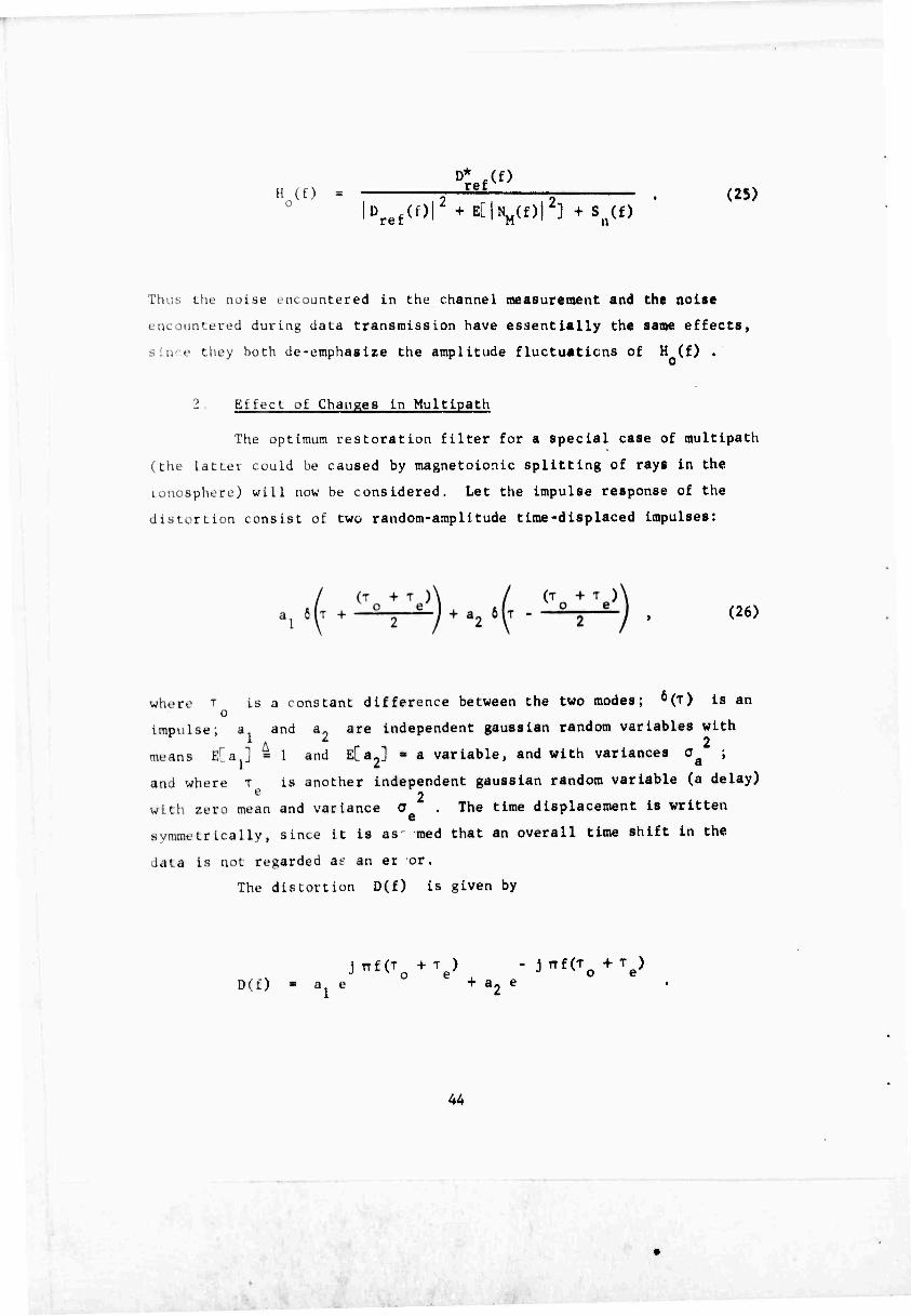
D* .(f) H(o - ■ =—^ = . (25)

o Dref(or + E[|NM(f)r] +su(f)

Tims the noise encountered in the channel measurement and the noise

encountered during data transmission have essentially the same effects,

slnoe they both de-emphasize the amplitude fluctuations of H (f) .

2 . Effect o£ Changes in Multipath

The optimum restoration filter for a special case of multipath

(the LatLei could be caused by magnetoionic splitting of rays in the

Lonoiphere) will now be considered. Let the impulse response of the

distortion consist of two random-amplitude time-displaced impulses:

where " is a

(26)

constant difference between the two modes; ^(T) is an

impulse; a and a„ are independent gaussian random variables with A 2

means Era,J = 1 and EfaJ - a variable, and with variances c ; 1 ^ ■

and where T is another independent gaussian random variable (a delay) • 2

with zero mean and variance a . The time displacement is written e

svmmetricallv, since it is as' med that an overall time shift in the

data is not regarded IC an er or.

The distortion D(f) is given by

JTTf(To+Te) -JTTf(To+Te) D(f) = a1 e + a9 e

The mean of D*(f) is

r. *, * ' J TTf T„ j TTf T E[D*(f)] = e 0 M(f) + E[a2] e 0 M(f)

M(f) is the characteristic function of the probability density of T

and is defined as

M(f) 4 .I." 32"£T.

For the gaussian random variable case assumed here,

2 2 2 - 2TT o r M(f) = e e

The mean-square value of D(f) is

E[|D(f)|2] = 1 + E[aJ + 2a 2 + 2 E[aJ M(f) cos 2nfT c • Z o

Assuming S (f) = 1 , the optimum restoring filter for the special a

multipath case is therefore

45

- 2 2 2n a e f2/-jTTfT JTTfTn\

[e 0-HE[a23 e 0) 11,(0 =- > --2-T2 * '(27)

2 2 -2TT 0 f I + 19 * + K[ü2 ] + 2 E[a2] e e cos 2nfTo 4 Sn(f)

2 lliis resiilr reduces to the known channel case if O and e 9

a are both zero. The effect of not knowing the differential delay ■ i

T between the two paths is made more clear in Fig. 11. In this

ti^'irc the magnitude of the restoration filter is plotted for the fol- 2

lowing parameters: a - 0 , S (f) - 0.01 , and a - 0.2/2TT . Note ' an e

that lor low frequencies, namely f < l/(2no ) , the filter is approxi-

mately an inverse filter; for high frequencies, however, the gain of the

tiller drops off. Thus for frequencies where the unknown variation In

the Jifferentlal delay of the multlpath Is not significant, the filter

uses amplitude Information; for frequencies where the unknown delay is

significant the restoring filter essentially discards amplitude Informa-

tion and relies only on the phase.

The effect of the unknown gain of the multlpath Is similar to

the effect of increasing the noise level. As a^ Increases, the

restoring tilter again places less emphasis on the amplitude.

C. APPLICATION OF SIGNAL RESTORATION TECHNIQUE TO HF BACKSCATTER

SOUNDING

The term "backscatter sounding" refers to forming an Image of the

radio reflectivity of the ground. This process Is completely analogous

to taking an aerial photograph of the ground thus forming an Image of

the optical reflectivity of the ground. Of course, different features of

the «round are prominent reflectors at the widely different frequencies

involved. While backscatter sounding sometLues refers to a technique

which gives the reflectivity as a function of range and radio frequency

at a fixed azimuth, in this study it refers only to the reflectivity as

a function of range and azimuth at a fixed frequency.

The analysis in the previous sections modeled the lateral

46

o o

FREQUENCY, f (Hzl

yrm

Figure 11 Amplitude of optimum filter transfer function | H0 (f)| .

(T is delay difference between two modes.)

47

variutiun c L' the amplitude and phase of a signal but not the variation

as a tuiu tion oi range. Experimental results relating to the range

variation an; not available. However because of the geometry of the ray

propagation, the correlation distance In range should be greater than

the lateral correlation distance.

The application ol the previous analysis to backscatter Imaging

requiiLv; interpreting time as representing an angle, and Interpreting

irequency as an Indicator of distance along the array. Improved angular

resolution is achieved by use of a reference to calibrate the amplitude

and pluisf vs dista.ice along an array. Scattercrs sufficiently close to

the retoronce are optimally processed by use of an inverse filter

(assuming a high signal to noise ratio). Scatterers far from the refer-

ence have an amplitude and phase which Is almost uncorrelated with the

reference and therefore the optimum filter uses only phase information.

In the Intermediate interval the optimum filter uses the amplitude

information only partially. The region which can be successfully

compensateil by the reference Is called the Isoplanatic region. This

region is not necessarily ilrectly related to the three regions pre-

viously defined. The practical problem Imposed by the optimum filter

is that its transfer function depends on the distance of the scatterer

from the image. In circuit theory this is equivalent to saying that the

impulse response depends on the time of the input. A further complica-

tion Is that this dependence Is a function of the statistics of the

amplitude correlations, which may not be precisely known.

A practical soiution requires the processing filter to be spatially

invariant. Thus a compromise filter which partially satisfies the re-

quirements hotii close to and far away from the reference is required.

In the absence ot noise, consider the effect of using an inverse filter

over all regions. The amplitude of the Inverse filter, 1/A(f) , can

cause an unbounded error in the region where the reference and the

scatterer are uncorrelated, and therefore might be useless for signal

restoration.

The use of the phase-only filter is near optimal far from the

reference, but suboptimal in the first region close to the reference.

48

In this first region the error Is in the amplitude A(x) . The

variance of A(x) is assumed bounded and therefore it is possible for

some array beam or image to be formed. Whether one should use the

phase-only filter or an approximation to the Inverse filter (which would

use amplitude information) depends on the degree of the distortion and

on how well one wants to do near and far from the reference. If the

distortion is not too great, then the phase-only processing may be

adequate close to the reference and the best one can do far away. If

the distortion is severe, then the phase-only pnnessing may be

inadequate everywhere and the best one can do is use the inverse filter

to restore signals very close to the reference.

In certain applications there may be physical reasons why the

amplitude distortion Is tot as bad as the phase distortion. For

example, In holographic Imaging only phase distortion is compensated by

the reference beam. Yet the quality of the reconstructed images made

from light propagated through atmospheric turbulence is good (see

Goodman et al.). Similarly, there may be conditions for which obliquely

propagated HF signals are distorted mainly in their phase characteristics

rather than In their amplitude characteristics. The proh1em of the type

of restoration filter to use is discussed again in Chapter V when an

experimental comparison Is made of including or excluding amplitude

information.

D. CALCULATION OF THE PERFORMANCE OF AN HF APERTURE WHICH USES A PHASE REFERENCE FOR SIGNAL RESTORATION

1. Case of a Fixed Array

In the previous section it was shown that compensating for

phase distortion improves the quality of distorted backscatter images.

The amount of the improvement is calculated in this section based on

a simple but realistic model of ionospheric irregularities. The model

does not Include amplitude distortion,and therefore compensation for

amplitude effects is not included in the analysis.

Define cp(x, y) as the phase difference between a signal

propagated from a source at coordinate y in the source plane and the

49

local oscillator of a receiver iltuated at coordinate x In the

receiving-array plane. These relationships have boen Illustrated In

Fig. I. Let the phtM f(x, Ay) measured at coordinate x In the

receiving array plane be defined as

<t(X| Ay) - cp(x, y ) - cp(x, y - Ay) a o

(28)

where y is the coordinate in the source plane of a scatterer or s r

sonrce wi ich is to be Imaged by the array, and y - Ay is the s

coordinate in the source plane of a reference signal.

In the previous chapter(see Eq. 6) the array performance

was shown to depend on a distortion function givei by

hLT(x) exp [-^(Ax)] Ax ■ x

where phase distortion cp(x) was the phase difference between the

array and the source at coordinate x . In the present case the phase

distortion is given by Hx, Ay) , since part of the distortion has bepri

asrumed to be cancelled by the reference. Therefore the distortion

function used for computing the array performance depends on i|r(x» ^y)

rather than on cp(x) . The distortion function for the case of a

reference, h ,(x) , is therefore defined to be ' ref

href(x) = exp [-^ (Ax)J (29) Ax

where D, (Ax) is the phase-structure function of \|i(x, Ay) given by

50

D^(Ax) - E[|t(x, Ay) - t(x - Ax, Ay)|2] . (30)

Substituting the definition of \|((x, A>) , Eq. (28), Into the expression

tov D.(Ax) , Eq. (30), and expanding the squared terms gives

Dt(Ax) - E||cp(x, ys) - tp(x, ys - Ay)|2|

+ E[|cp(x - Ax, ys) - cp(x - Ax, ys - Ay)| |

-2EJ{9(x. y8) - <p(x, ys - Ay)}{cp(x - Ax, ys) - cp(x - Ax, ys - Ay)}|

The correlation function of the phases of two signals transmitted from

points separated by Ay and received at points separated by Ax Is

defined as

K (Ax, Ay) » E[cp(x, y) cp(x - Ax, y - Ay)] . (31)

Using this definition, D.(Ax) can be rewritten as

yAx, Ay) - 2^(0, 0) - 2^(0, Ay) + 2^(0, 0) - 2^(0, Ay)

(32)

2K (Ax, 0) - 2K (Ax, 0) + 2^(Ax, - Ay) + 2^(Ax, Ay) .

The correlation function In Eq. 31 Is difficult to evaluate.

The difficulty In the analysis occurs If the rays of two signals cross

51

in tin' lüuusplitrc as Illustrated La Plgi 12. 11 the lünosphere is

modi'U'd aa a thin screen of Lrregularltltl the crossing rays should

have highly cotrolaiod pliases, since the perturbations introduced by

the lonüsphci-c slum Id be the same for both ray». If on the other hand

the iüiiuspherc is mode'^d as a thick screen of irregularities, then the

phase correlation of the crossing rays is low. In the analysis to

follow an a. sumption Is made which corresponds to the thick-screen,

low-correlation cuse, Fig. 12b. This assumption is made because It

greatly slmplltles the analysis and because It gives a lower bound on

llio array performance. If the crossing rays of the reference and the

source ar»« In fact more correlated than is assumed In the following

model, the effect of the Ionospheric distortlon would be less than that

predicted by the equations to be derived. This Is so since a high

correlation implies that the reference signal is more effective at

compensating for the phase distortion than It would be for a low

correlation. (See Gasklll ^ for a similar discussion of thiß

approximation.)

The correlation function K Ux, Ay) defined in Eq. (31)

assumed here Li even and symmetrical In Ax and Ay and is given by

^(Ax, Ay) 2

acp exP (AX)

2 t tkül (33)

Substituting this definition, Eq. (33), Into the expression for D.(Ax) ,

Eq. (32.1, It Is found that

^ ^x) ■ 4a 1 - exp exp .(*)1 (34)

This phase-structure function can be rewritten as

52

SOURCt PLANE

ARRAY PLANE

(•I IONOSPHERE MODELED AS A THIN SCREEN OF IRREGULARITIES (High PtwM Corralationl

(b) IONOSPHERE MODELED AS A THICK SCREEN OF IRREGULARITIES (Low PhtM Corr«l«ionl

Figure 12 Rays crossing among ionospheric irregularities.

53

^ ^x) 2c I - l-'Xp (35)

WhlTt'

20 ' 1 - exp [■W (36)

This torm of D, (Ax) makes It roscmhle the form of D (Ax) In Eq. Sb, I 2 T

except that an equivalent phase variance C ^ Is substituted for the 2

actual phase variance a . In Figs. 8 and 9 It was shown that the

periurmance oi an array depends on this plnse variance. Equation 36

«ives; an explicit expression for determining how the performance of the

arrav depends on the separation Ay of the reference from the point to

be imaged. As the point to be imaged gets closer to the reference, 2

Ay—»0 , the equivalent phase variance 0 approaches zero, 2 e

0 —»0 . Thiis the problem of determining the Improvement in array

performance afforded hv a phase reference has been reduced to an already 2

solved problem by defining an "equivalent phase variance", ü

An approximation valid for large phase variance a can be 2 '

made which makes the expression for a easier to interpret. For 2 2 e

cp

exp

therefore 9 , Eq. (36), can be approximated by

m 2o Ail ■ (37)

54

In Chapter II It was shown that the equivalent rms phase should be less

than 1/4 cycle to avoid dlstort'on of the mean array power pattern.

For the case of large rms phnse, the distance Ay between the

reference and the point to be Imaged should be smaller than

*- 2TTA ..,„. by $ 2/20 • ()8)

It was noted In Chapter II, Eq. 9b, that the rms angle of arrival a^

was given by 0

0 \ 0e '

0 /2 2TT A

Using this equation the expression for resolution of Ly can be

rewritten

o

Thus the size of the region which can be Imaged with little distortion,

expressed in units of wave lengths, Is Inversely proportional to the rms

angle of arrival. For example, If the rms angle of arrival Og is 1 0

1/4 deg (.004 rad) which has been observed by Sweeney , and the wave

length is 20 meters, then Ly should be less than 2.5 km.

55

2 . Casi' oi ,i Synthol ic A|)erttire

It will now be shown that the use of a phase reference

mprovos tlie pu ft oimaiKe ot a syntlietlc aperture in exactly the same way

t opt'ralo;; tor Chf t ixcJ aperture. Namely, the effective phase variance

■ ivducod by an anumiU whicii dopeuiis on the separation of the reference

ami tht loured Tlic eltecive correlation distance of the phase is also

reduced depending on Ch« U'inporal time constants and the velocity of the

entenne. An equivalent scalo size is defined exactly as It was in tlio

analysis of the synthetic aperture without the reference.

The array performance is determined by the phase-structure

function of i (x) (see Eq. 30) which is given by

MAx) = E[|Hx, Ay, t) - t(x - Ax, Ay, t - At)|Z] , (40)

where At ■ Ax/v a

and t(«i Ay, t) = cp(x, ys, t) -9(x, yg -Ay, t) .

This definition of i|f includes temporal effects and is a straight-

forward extension of the definition used in the previous section.

Evaluation of this expression gives

D (Ax) ■ 2KT(0, 0, 0) - 2KT(0, Ay, 0) + 2KT(Ax, 0, At)

^ ' (41) KT(Ax, y, At) - KT(Ax, Ay, At) ,

where

56

K (Ax, Ay, At) = ^(x, y, t) cp(x - Ax, y - Ay, t - At)] (42)

Using the same justification employed in previous sections,

the correlation of the phase of two signals transmitted and received at

different points at different times is assumed to be

KT(Ax, Ay, At) = 0 exp kj - fey ■ if)2 (43)

Substitution of this correlation function into the expression for the

phase difference structure function yields

Df (Ax) 2a (44)

where = 2a ' ■m

21

(45)

and J^ = i + —L. 2 2 2 ' A ^ A^ (v T) e v a '

(46)

Note that the equivalent irregularity scale size A is

relevant only for the array coordinate Ax ; the actual scale size A

is relevant for the separation of the source and the reference, Ay .

For example, consider the situation where the spatial

irregularities are very large, A ^ o0 , but there are temporal varia-

tions with correlation time T . In this case the equivalent correlation

57

distance A is given by A = v I ; however, the equivalent phase

variance is zero, 0 « 0 . Thus the array pattern is not distorted at

all because the reiercnce compensates for all of the phase variations.

The conclusion of this analysis of a synthetic aperture using

a phase reference is that: the results for the equivalent fixed array,

without a reference, can be used if the phase variance and irregularity

scale size are replaced by an equivalent phase variance and an equivalent

scale size. These quantities [see Eqs. (36), (46)] depend on the

velocity of the moving antenna used to synthesize the aperture, the time

constant of the ionospheric phase variations, and the distance of the

source from the reference.

3. Evaluation of the Analytical Results for Typical Ionospheric Parameters

The properties of signals propagated over an oblique

ionospheric path are quite variable, depending on the path geometry,

solar activity, and time of day. It is instructive, nevertheless, to

attempt to evaluate the array performance using parameters of iono-

spheric propagation which are reasonable. From this attempted evalua-

tion, one can gain better insight as to what a realistic array perfor-

mance might be.

The parameters necessary for the calculation are given in

the following table:

Spatial Correlation Distance A 20 km 1

Temporal Correlation Time T 60 sec j

Rms Phase Distortion a 9

V a

3(2TT) radians

Airplane Velocity 100 ra/sec ]

Wave Length X 20 m |

These parameters give an rms angle of arrival ag of

58

1/4 deg which is consistent with observations made by Sweeney. These

parameters also give an equivalent scale size A , see Eq. 46, of 6 km.

It was shown in Chapter II, Eq. 16, that if the rms phase is greater

than one cycle, the aperture length is limited by the following

equation in order to avoid significant distortion:

L < _2A a

For the parameters given above this is about 20 km for fixed aperture

and about 6 km for a synthetic aperture.

If compensation for distortion Is provided by a reference,

then it is important to determine how far from the reference an imaging

point may be and have the array power pattern essentially undistorted.

In the discussion following Eq. 39 it was shown that for an rms phase

angle of arrival, aQ , of 1/4 deg, a point to be imaged should be öo

within 2.5 km of the reference in order to avoid distortion. Thus, for

the parameters given above, the region surrounding the reference which

could be imaged without distortion is quite small.

59

gmr — f »HI in .H«riii|ii—-■o^« *

■•<.^^l

■

(

BLANK PAGE

■

-i— •«■iMHWMdb Mhi

■

IV. DESIGN OF THE HF SYNTHETIC-APERTURE EXPERIMENT

The purpose of the experimental program was to ascertain the

ability of an HF synthetic aperture to achieve high resolution in the

reception of ionospherically propagated signals from a distant source.

An objective of particular interest was to investigate the usefulness

of an HF synthetic aperture in detecting and resolving backscatter

signals. The latter are ionospherically propagated echoes caused by

the reflection from distant areas of HF radar signals beamed to these

areas by an oblique-incidence "sounder" (transmitter) located near the

receiving array.

In much of the experimental program, backscatter echoes from an

area about 2600 km from the synthetic aperture were studied. Localized

enhancement of the backscatter signals at two specific points was

simulated by the use of repeaters located at these points. One of the

repeaters was also jse.i to provide compensating and reference signal

features. The ultimate aud most important objective of the experimental

program was to find out to what degree of resolution signals from the

two distant repeaters could be distinguished from each other by the HF

synthetic aperture.

The experimental program was designed to identify key technical

problems, evaluate their significance, suggest solutions, demonstrate

the basic feasibility of the synthetic-aperture technique, and determine

operational and other limitations.

A. BASIC COMPONENTS OF THE EXPERIMENTAL SYSTEM

The principal components of the system used in the experimental

program were:

1. A medium-sized twin-engine aircraft equipped with receiving and recording equipment and flying an approximately north-south path near Los Banos, Calif, (see map. Fig. 13). This aircraft and its equipment constituted the HF synthetic aperture.

61 Preceding page blank

a>

E I

i

I

M

CO

2. Two CW transmitters near the flight path which provided airplane tracking signals.

3. A CW transmitting source at Bearden, Ark., approximately 2600 km from Los Banos for use in the "forward-propagation" experiment.

4. Two repeaters (one fixed, one portable) at Bearden.

5. A high-power, narrow-beam transmitter at Lost Hills, for use as an "oblique-inridence ionospheric sounder" in the backscatter experiments.

6. A ground-based digital computing facility used for off-line signal processing.

These system components were utilised in the experimental program

now to be described.

B. PRINCIPAL FEATURES OF THE EXPERIMENTAL PROGRAM

The essential steps in the experimental program were:

1. Verification of airplane tracking subsystem performance.

2. Measurement of beam width achievable with the synthetic aperture when it was receiving a CW signal transmitted from Bearden (the CW forward- propagation experiment). In this test compensation was applied for deviations of the airplane from a linear flight path by the use of the airplane tracking data.

3. Demonstration of feasibility of obtaining two- dimensional backscatter data (range vs cross range) without compensating for ionospheric distortion or deviations of the airplane from a linear flight path.

4. Investigation of the use of an HF repeater at Bearden to provide a reference signal in compensating for airplane flight path deviations and ionospheric distor- tion, for the purpose of obtaining extremely high azimuthal resolution in backscatter mapping.

C. SYSTEM DESIGN

A 100 km aperture was synthesized near Los Banos in the San Joaquin

Valley of California (see map. Fig. 14). The aperture used a DC-3

63

Figure 14 Detail map showing flight path In relation to Los Barfos and to location of CW tracking transmitters.

64

aircraft which flew at approximately 180 mph (80 m/sec) for about 20

minutes per flight. The airplane was equipped with a horizontal and a

vertical tubular alumir.nm antenna. A complete swept-frequency CW (SFCW)

receiving system plus an analog recorder were Installed in the craft.

The signal was a linear FM sweep, centered near 2C MHz. The sweep was

repeated every second, covering a 600 kHz band width at the rate of

1.0 MHz/sec. This sweep provides delay resolution of about 3 M^sec.

The flight geometry and signal design resulted in a potential range and

cross-range resolution of about 500 m in the backscattet observation

area and guaranteed freedom from array grating lobes (multiple side

lobes) within the area illuminated by the backscatter sounding trans-

mitter. The latter was located at Lost Hills, Calif., at a distance of

approximately 200 km south cf the synthetic receiving aperture. This

equipment can transmit a full 30 kW in a 4 deg beam width, using the

SFCW signal described above. A detailed description of the equipment

components is given in Appendix A.

Compensation for ionospheric and aircraft-motion effects was

provided by measurements made on a signal returned from the fixed re-

peater in Bearden. The repeater is a receiver and transmitter combina-

tion with separate antennas and is used to rebroadcast signals in the

frequency band of interest. The amplitude and phase of this strong

signal were used in this experiment to compensate for distortion of the

backscatter signals.

In order to separate the distorting effects of the ionosphere from

those caused by aircraft motion, it is necessary to know the airplane

flight path with high accuracy. To meet this requirement two CW trans-

mitters were located on the ground within line of sight of the flight

path; their signals were received and recorded on the plan?. (See

signal diagram, Fig. 15.) In addition, a precision differential aneroid

altimeter was mounted in the plane and its output recorded. An aerial

camera mounted on the aircraft provided aerial photographs from which

the aircraft position coordinates were determined by photogrammetrir

reduction at the beginning and end of each flight.

Use was made of the ionospheric sounding capability of the Stanford

65

FLIGHT PATH

DOPPLER

TRANSMISSION (CW)

DOPPLER TRANSMISSION (CW)

CALIBRATION SIGNAL

o LOS BANOS

RECEIVER AND DOPPLER TRANSMITTER

SITE

BACKSCATTER SIGNAL

"21 BACKSCATTER

SIGNAL

o LOST HILLS

TRANSMITTER

SITE

SFCW TRANSMISSION

Figure 15 Diagram of signals for synthetic-aperture experiment.

66

Radiosclence Laboratory, whose equipment includes the SFCW generator and

repeaters in Bearden, Arkansas, plus a wide-aperture linear receiving

array and processing equipment at Los Banes. Thus it was natural to

make Los Banos the control center for the operational aspect of the

expeiimert.

As already noted, the forward-propagation experiment used CW signals

transmitted from Bearden. The operating frequency of the CW signal had

to be selected to make sure that only a single ionospheric propagating

mode was used. This mode was the one-hop lower ray cf the F layer.

Compensation for airplane motion was essential to the forward-propaga-

tion experiment and was provided by the method already described. The

CW measurements were made indepe' iently of the backscatter measurements,

although much of the equipment was the same.

D. SYSTEM PARAMETERS

I. Backscatter Experiment

The backscatter system parameters were determined from value

tradeoffs among considerations of achieving a small cross range resolution

cell (defined as range times azimuth), reasonable aircraft velocities, and

processor complexity. A range resolution of 2 or 3 l^sec can be achieved

reasonably often without dispersion compensation. An aircraft velocity

of 180 mlles/hr seemed reasonable. The ground resolution cell was

therefore established to be about 500 m In range and 500 m in azimuth

at a range of 2600 km. A square resolution cell appeared appropriate

for the purpose of mapping, since increasing resolution in only one

dimension does not seem necessarily to Improve the interpretabllity of

the map. It should be possible to extend the resolution of the system

by Including some dispersion compensation and using a faster aircraft

and longer flight paths. However, the 500 m x 500 m resolution is an

Improvement of more than an order of magnitude as compared with that

achievable In the present state of the art, and appears to be good

enough to obtain usable ground maps and ionospheric data.

A range resolution of 500 m corresponds to a time-delay

resolution of about 3 M-sec. This in turn requires at least a 0.3 MHz

67

band width, ihu »»Imuthal rt'solutLon of 500 m (AA) corresponds to a

l light, palh of about L ■ T* ■ 100 km for \ = lb m , R = 2600 km ;

or an angular rtiolutlon of 1.5 x 10' radians for a half minute of arc.

An improvemonl in angular resolution by a factor of two could be achieved

by installing the backscaLLer transmitter in the airplane; however this

would greatly ijompl icate the design.

With the system band width determined at about 0.5 MHz and

the synthetic aperture length determined at 100 km (2: 60 miles), the

next issue to consider was the type of pulses to be used, and their

period. IfCM was chosen for good range resolution and high average

signal energy. The pulse repetition frequency (PRF) and the duty cycle

of the pulses are determined by three factors:

1. The sweep rate.

2. The energy desired per pulse.

3. The spacing of the array grating lobes.

The array grating lobes are secondary lobes due to spatial

aliasing which occur when the elements of an array are spaced by more

than a fourth of a wave length. For the experimental system, as much

energy as possible was desired, and the grating lobes should be spaced

by at least 10 deg, since the available transmitting antenna had a 4 deg

beam width. This result requires about 1000 pulses for the synthetic

array (equivalent to 1000 array elements in a stationary array). If the

aircraft velocity is 180 mph and the signal length is one-half second,

the sweep rate required is 1 MHz/sec. The nominal parameters of the

system are summarized in Table 1.

Another Important parameter of the system is the degree of

phase coherence required. The timing and frequency standards at the

transmitting site and in the aircraft must be synchronized, and all

oscillators must be phase-locked to these standards.

Tne basic requirement for the frequency standard is that its

phase should drift by only an insignificant amount in the 20 minutes it

takes the aircraft to fly the aperture. The exact meaning of

68

TABLE 1

PARAMETERS OF BACKSCATTER EXPERIMENT

Aperture length 80 km

Approximate wave length X 15 m (center frequency 20 MHz)

Pulse length 0.5 sec

PRF 1 pps

Signal ceding SFCW

Band width 0.5 MHz

Range resolution 3 M-sec ( m 500 m)

Azimuthal resolution 1.5 X 10"4 radian m 0.5 minute o f arc

Lateral resolution in far field (2600 km) 500 m

Grating-lobe spacing ± 10 deg

Sweep rate 1 MHz/sec

Airplane velocity 80 m/sec

Flight-path duration 17 min (1000 sec)

Transmitted power 30 kW

Transmitted beam width 4 deg .

69

"insignificant" depends on the nature of the phase drift. No signal

distortion results if the phase drift is linear; if the drift is a

quadratic, it should be less than one radian. If the drift is periodic

or completely random, a more careful analysis is required. Long-term

stability of a cesium-beam frequency standard is specified to be a

drift in frequency of less than one part in 10 . The short-term drift

of such a standard, measured over 1000 seconds, is specified to be less -12

than 2 x 10 , which at 20 MHz is about 14 deg. The short-term

stability is therefore sufficient for the synthetic-aperture experiment.

However, it is to be noted that a less stable standard would not

necessarily be sufficient.

The dynamic range of the entire system is quite high because

of the two-dimensional Fourier-transform processing described in Section

F. The conversion from demodulated SFCW to range information (a one-

dimensional Fourier transform) is equivalent to passing the signal

through a bank of 2 Hz filters. The increase in ratio of signal voltage

to noise is equal to the square root of the ratio of the receiver pass-

band to the analysis passband. This band width ratio is 6000/2, giving

a signal-to-noise ratio increase of better than 30 dB. The formation

of a beam by the aperture improves the voltage signal-to-noise ratio by

the square root of the number of synthetic elements (or equlvalently by

the square root of the number of pulses integrated). The design is for

a 1000-element array; therefore the improvement Is 30 dB. The 40 dB

signal-to-noise ratio of the receiver and analog recorder bring the

overall system signal-to-noise ratio to 100 dB.

This signal-to-noise ratio is only relevant to the strongest

backscatter signal, which is generally that from the fixed repeater.

The system dynamic range is much larger than the range of backscatter

intensities which one might want to image in a feasibility experiment,

and is also much greater than the self noise due to side lobes. The

latter arises as follows: Phase errors vs frequency (in the SFCW)

introduce range side lobes, while phase errors in the synthetic aperture

give angular side lobes. The side lobes cause backscatter returns at

different ranges and angles (cross ranges), with the result that they

mutually Interfere. The effect is similar to that of noise, and has 29

often been called "self noise". (See Evans and Hagfors for a review.)

The design goal is to keep the amplitudes of the side lobes 30 dB or

more below tbJ peak amplitude of the main lobe. Thus, at the least,

large variations in the backscatter intensity should be visible.

2. Forward-Propagation Experiment

The parameters for the CW forward-propagation experiment were

established by the parameters of the backscatter experiment. The only

new parameter of interest is the stability of the clock at Bearden. It

was not expected that apertures longer than 20 km would be synthesized

in this portion of the experimental program; therefore, the stability

requirement on the standard is not as great as it is for the backscatter

experiments. A crystal frequency standard was used which had a speci-

fied stability of 10 for averaging times of 1 sec to I hour. Over

the 200 sac the airplane requires to fly a 20 km path, the phase error

on a 20 MHz signal is about 130 deg. Since most of this error is ex-

pected to consist of a drift which does not distort the array beams but

only skews them in angle, this phase error was judged acceptable.

E. FLIGHT-PATH ACCURACY AND MEASUREMENT

Unknown deviation from a straight line in the aircraft flight path

degrades the performance of the synthetic array. A random error of a

radar wave length (15 tn) from pulse to pulse would make it essentially

impossible to process the data in such a way as to obtain an effective

narrow beam width. A sinusoidal flight-path variation causing a phase

change of 6 deg (0.25 m) can produce a single "error" side lobe about

26 dB (0.05) down from the level of the main lobe. A random phase error

with rms value 6 deg can produce a hash side lobe level about 60 dB

down (0.05/ / 2000). Because the structure of the phase variation cannot

be specified, it is necessary to set as a design goal the tolerance

which guarantees a good main lobe width and side lobe level. Thus a

6 deg tolerance is specified, corresponding to a lateral distance of

71

Ax — ^Q = 25 cm, or a nominal flight-path accuracy of one foot. The

height accuracy required is not as severe because the angle of arrival

of the ray will be about 10 deg from the horizontal. The height re-

quirement is therefore l/sin(10 deg) or about 5 ft.

It is not required that the flight path be linear to this accuracy,

but rather that the flight path be measured to this accuracy. The

pliast. variations, if known, are removed during the digital processing

stage.

Twc techniques for measuring the flight path were employed. One

makes use of an aerial camera mounted on the aircraft. This camera,

providing about 5 ft of resolution in ground track, was used to estab-

lish the starting reference for the CW tracking system.

The second system employed an aneroid altimeter and two CW 'rans-

mitters, one located in line with and the other perpendicular to the

flight path as shown in Fig. 14. These signals were received in the

aircraft and recorded on analog magnetic tape. The recorded signals

were digitized at a later time and processed by a small general-purpose

digital computer to obtain the coordinates of the airplane as a function

of time. The CW signals were in the HF band above the critical fre-

quency of the ionosphere.

The orientation and altitude of the flight path were determined by

several considerations. The altitude had to be set to guarantee a line-

of-sight path to Los Banos (a CW tracking station) but not to Lost Hills

(in order to suppress the direct SFCW signal from the latter). The

compromise arrived at an altitude of 6000 ft. This altitude was also

satisfactory for the aerial photography.

The flight-path orientation was set to pass over flat land and in

line with Los Banos, so that the CW signal from Los Banos could be used

directly to measure ground speed. The path could not be too close to

Los Banos because large changes in the strength of the CW signal would

then result as the plane flew the path. Nor could the path be too far

fron Los Banos, because the CW signal would then be too veak because

of propagation loss and shielding from the earth.

72

'' ■* ^ ■■'«••.■ . '

F. DIGITAL SIGNAL PROCESSING

Digital data processing was used to make a two-dimensional

backscatter map from the sequence of demodulated SFCW received signals

which were produced by the synthetic-aperture experiments. The recorded

signals were bandpass filtered and then sampled at a 5 kHz rate. The

samples were converted from analog to digital form (A/D) and were re-

corded on digital tape using a Sigma 5 computer. 4096 samples were

stored in one tape record each second. (904 samples wero discarded

every second. These correspond to the interval when the transmitter was

off.) A total of 1024 records were made, which corresponded to about

17 minutes of data. At an average aircraft velocity of 80 m/sec,

these data represented a coherent synthetic aperture about 80 km in

length. The details of the signal process are presented in Appendix B.

The data group for each sounding pulse represented an element in

the equivalent stationary array. Each demodulated SFCW signal was

Fourier-transformed to produce information on amplitude and phase vs

delay.

The second part of the computer signal processing took one range

bin at a time and combined the data for each synthetic element, i.e.,

amplitude and phase vs distance, to form a record of amplitude vs angle.

The processing was a Fourier transform in most cases. However, a more

general form of coherent addition had to be used in some cases and is

explained more fully in Appendix B.

Because the aircraft velocity variations were not insignificant,

the spacing of the equivalent stationary array elements was not

uniform. Aircraft tracking data were available, and have been used in

some cases to compensate for the longitudinal variation in the equiva-

lent array-element position. This compensation is a function of the

cross range from the reference to the point to be imaged, however, and

therefore further complicates the coherent summing operation.

The Fourier-transform processing was implemented on an IBM 360/67

computer and was designed to be as flexible as possible. It Is possible

to use less than the 1024 equivalent elements available, or to compute

a partial backscatter map.

73

-. v ..-..■ .

The program output was made available in several forms. One form

of output was on magnetic tape which can be read by the Sigma 5 computer.

Thus the output data are now stored on tape and can be replotted in any

format. The principal Sigma 5 display was three-dimensional and was

drawn by a computer-controlled plotter.

The digital processing for the CW data from the forward-propagation

experiment was much simpler than the processing for the backscatter data.

At the A/D conversion process, the amplitude and phase of the CW signal

at one-second intervals were measured and recorded on tape. A second

program, written for the Sigma 5, was analogous to the beam-forming

program for the backscatter; it essentially executes a Fourier transform.

Aircraft tracking data were incorporated into the beam-forming program

(see Appendix B).

74

■ ■■■■■■■!■ ■ ,■ . . ■ . ■ !..■ :,,,,,.., ;

■

V. RESULTS

In Chapter IV, the principal features of the experimental program

were outlined. The results are described below.

A. VERIFICATION OF AIRPLANE TRACKING SUBSYSTEM PERFORMANCE

The airplane tracking subsystem, used in the CW forward-propagation

measurements, proved to be quite accurate. On four different flights a

comparison was made between the location of the airplane at the ground

markers at the ends of the flight path (which are separated by about

60 km) as measured by the radio system, and as measured by the photo-

grammetry. The flights used for the tracking verification were Flights

2N, 2S, and 3N on ?? April 1,69, and Flight 3S on 26 April. Detailed

data are presented in Table 2 at the end of this chapter.

The location errors were found to be 20, 25, 35, and 60 m,

respectively, for the above flights. Thus the long-term average error

was quite small.

A plot of the lateral deviations of the plane from a straight line

that represents a mean-square best fit for position data for the entire

flight path is shown in Fig. 16 for Flight 3N made on 22 April 1969.

To aid in evaluating the effect on antenna performance, the rns devia-

tion of the position data from straight-line segments is determined.

The curve is divided into 32 segments of 32 seconds each, 16 segments

of 64 seconds each, and so on to two segments of 512 seconds each. For

each of these segments a mean-square best fit straight line is deter-

mined. The rms deviation of the curve from the straight line is then

measured. The minimum, average, and maximum rms deviations for the

group of segments of each length is plotted in Fig. 17. These numbers

can be used to determine whether it m'.ght be possible to use a certain

length time interval in forming a synthetic aperture if compensation

for the plane motion were not used. However, it appears that even with

a lax requirement such as 0.2 X for rms variations from a straight

line, an aperture of less than 3 km might be the maximum possible at

75

z o p < > UJ 0

400 A 1 1 1 1 1

FLIGHT 3N

1 1 1 1

—

300 " \

22 APRIL 1969 / \

H

200 - \ / n A

100 - \ / ^

-]

o \ A I A i / \ i i i i / i i i

v /\ f \ 1 \ / ^-BEST FIT

-100 - \

/ LINE A

-?ro - \ jJ -]

-300 - \ / -\

-400

-RDO 1 1 1 1 1 1

-]

100 200 300 400 500 600 /OO oOO 900 1000 1100

FLIGHT TIME (seel

Figure 16 Deviations of flight path from straight line that represents mean- square best fit for position data taken over entire flight path.

76

■

■ ■■ S IU ■ :■■-■ ■. :■ . ... . .;..,. ■ ■ - ■ -■

O) r

4-

c o

4-» c

Q. 0) 0)

m s y c </) — 3

o 4^

en (15 > 01

w 1 Mw o O

c a>

3> .* L, 3^

CO

03 4-J TO to

"0 *~ | 0 c s. n u.

r '<7) IS *-» u g a r a ü)

•M n £ *^ di)

5^ en 4-»

E 1

I

S 8 8 S 9

(ui) NOIXVIABQ SNU

.2 a, 'S ^ r1 to ro ^ 'ill

oc E i^

I u.

77

i ^B .,»- !.v=a*«» ■

K m 20 1 compensatton for flight-path deviations were not applied,

B, CW FORVsfARD-PROPAGATION MEASUREMENTS

The frequency spectrum of the CW signals transmitted on a one-hop

F-mode (lower ray) from Bearden, Arkansas and received either at Los

Banos or in Che airplane were calculated by Fourier-transforming the

data in time intervals of certain lengths. The frequency spectrum

determined from the data received at the fixed Los Banos site give an

indication of the temporal variations of the ionosphere. These temporal

variations limit the processing time which can be used, or equivalently

the frequency resolution which can be obtained. The frequency spectra

determined from the data received in the airplane give an indication of

the spatial and temporal variations of the ionosphere. The forward

motion of the plane produces a synthetic aperture, so that the frequency

spectrum is equivalent to an angular spectrum, as was described in

Chapter II. Thus the temporal and spatial ionospheric variations limit

the angular resolution that can be achieved by the synthetic aperture.

The experimental results determine what these limitations are for favor-

able ionospheric conditions and give an Indication of the relative

importance of the temporal versus the spatial variations of the

ionosphere.

It is essential in these CW measurements that random deviations of

the airplane from a straight course be compensated for in order that

variations induced in the data by these deviations not be confused with

variations induced by ionospheric irregularities.

About 1300 sec of data from run IS on 24 April 1969 (see Table 2)

were analyzed. On this day the geomagnetic activity was quiet. (See

Table 3 at end of chapter.) The CW frequency for this run was 23.3 MHz.

The data from the horizontal antenna of the airplane and from Los Banos

were processed in time intervals of 32, 64, 128, and 256 seconds. In

almost all cases the 32 sec frequency spectra were nearly ideal. The

typical and best frequency spectra for the signal received at_ Los Banos

for 64, 128, and 256 sec processing intervals are shown in Figs. 18, 19

and 20 respectively. The theoretical 3 dB frequency resolution is

78

1.0 —

1= JE „ 0.8 ü „ ü fe8 0.6

I" 0.2 —

0.0

1 1 1 1 1 1 1 1 1

l— U) BEST RESULT

III

1 —\

1 i i WwV« 1

1.0

1 1 1 1 1 1 1 1 1 1 1 1

— (bl TYPICAL RESULT i —1

i: «>-8 1 —J

II g St 0.6 — t 1

jl M — 1

I —j

0.2

0.0 VVvi/^ 1 45 40 35 30 25 20 15 10 5 0 -5 -10 -15

FREQUENCY RELATIVE TO BEAROEN SIGNAL (In Units of 1/64 Hz)

Figure 18 Frequency spectrum of forward-propagated CW signal received at Los Bands—64 sec processing time.

79

10

08

la) BEST RESULT

5 a _ fi - K u OJ . a. ■ 5) i'

O 9 06

Q & 3 i

a. o

<

04

0.2

0.0 ■^■r ■ '^\^.\\{.y -.. ..^. . ^.^x^r^-^^^^^iv^^ | MWI^IW^VVAV

5 D - x -

m s.

10

0.8

0.6

— (b) TYPICAL RESULT

Q B

il 04 <

0.2

0.0

1—I—r

^-VXl^^^s-v^^^^JvA^^v-^VM^JV^^ I ^Wwwiv^A 45 40 35 30 25 20 15 10 5 0 -5 -10 -15

FREQUENCY RELATIVE TO BEARDEN SIGNAL (In Units of 1/64 Hz)

Figure 19 Frequency spectrum of forward-propagated CW signal received at Los BaiTos—128 sec processing time.

80

>■ .,

. ...,,...,,..,.-..,.,. —.

1.0

5

1 1 1 1 1 ' 1 1

— (a| BEST RESULT

III

1- |; o.8

n O 8 0.6 —

0.2 - "

0.0 A*^lwuJ../Wwl^^Ju^^^ 1 K*-MWUv^,

1.0

s 3 _ DC ••

— (b) TYPICAL RESULT

I "- a O » 0.6

11 II <

0.4

0.2 —

0.0 VA4r-V^^vWA^ 45 40 35 30 26 20 15 10 5 0 -5 -10 -15

FREQUENCY RELATIVE TO BEARDEN SIGNAL (In Units of 1/64 Hz)

Figure 20 Frequency spectrum of forward-propagated CW signal received at Los Bands—256 sec processing time.

81

L/T , where T is the processing time. Thus for the 128 sec

processing time the 3 dB width of the frequency spectrum is about

0.008 Hz.

The typical and best frequency spectra (or equivalent angular

spectra) for the signal received in the airplane for 64 and 128 sec

processing intervals are shown in Fig. 21 and 22 respectively. The

nominal airplane velocity was 75 m/sec and the wave length was about

14 m. Thus the 128 sec processing time gives an angular resolution of

14/(128 x 75) = 0.0014 radians or about 0.08 deg. The equivalent

aperture length is 9.6 km, which is longer by a factor of four than the

Los Banos phased array.

The results for this data are summarized in the following table.

SUMMARY OF CW RESULTS

Los Banos receiver

Airplane receiver

Processing time (sec)

64 128 256

20/27

12/21

7/13

2/10

1/5

0/5

Numerator = number of cases for which nearly ideal frequency (angular) resolution was achieved. Denominator = total number of cases.

Additional measurements were also made for Flights 2S and 2N on

22 April 1969, IS on 24 April 1969, and for 3S on 26 April 1969. The

results for these other flights are essentially the same as those shown

in the above table for Flight IS on 24 April 1969. The airplane speeds

for all the above runs were between 56 and 88 m/sec. The results did

not appear to depend in a direct way on the airplane speed.

These results are interpreted as indicating that the theoretical

ideal beam width of a 5 km aperture was achieved in about 50 per cent

82

■: r ' :■■' '■ "'■■■■■

p.3ge 83 intentionally blank

1.0 —

1 1 1 1

la) BEST RESULT

i i i i 1 1

1

i" 0-8 — —

SI "> a.

S S 0.6 — —

RI t- 2 Si 5 0-4 — —

lä - -

0.2 — A

0.0 '-vyVrvr--fv .-^VlA^WV V W)^

3

i 1 Q N if ii

1.0

1 1 1 | 1 1 1 1 1 1 1

- (b) TYPICAL RESULT _

0.8 —

0.6 1

0.4 —

0.2

0.0 ^V 45 40 35 30 25 20 15 10 -5 -10 -15

AZIMUTH ANGLE RELATIVE TO DIRECTION OF BEARDEN (In Units of X/64v. Rad)

Figure 21 Angular spectrum of forward-propagated CW signal received in airplane- 64 sec processing time, equivalent to 5 km aperture.

The angular spectrum is equivalent to the frequency spectrum. 1/64 Hz represents X/{64 vj radians or about 0.16 deg for the parameters of the test.

84

-•„re, -.,7'*--,

1.0

1 1 1 1 1 1 1 1

— (a) BEST RESULT

I I

1

ir O-8 _ o "

o 8 0-6 — —

Si *1 3 1 0.4 — — ll <

0.2

0.0 r lJ <

f

i« UJ J< n O N

||

ii <

1.0

1 1 1 1 1 1 1 1 1 1 1

- (b) TYPICAL RESULT

0.8 — -

0.6

A

i

0.4 j / r

. 1 1

0.2

0.0

45 40 35 30 25 20 15 10 -5 -10 -15

AZIMUTH ANGLE RELATIVE TO DIRECTION OF BEARDEN (In Units of X/64va Radl

Figure 22 Angular spectrum of forward-propagated CW signal received in airplane- 128 sec processing time, equivalent to 10 km aperture.

85

■

of the cases tested, while the theoretical ideal beam widtii of a 10 km

aperture was achieved in about 20 per cent of the cases tested.

Although the frequency spread of the data received in the airplane

is not quite as narrow as that received at the fixed.site, the time

variations of the ionosphere appear to be a significant factor in

limiting the beam width achieved by the synthetic aperture. It is un-

likely that the aircraft flight-path deviations are the cause of the

frequency spread. It was shown by checking the tracking data with the

photogrammetry results that the long-term tracking error was exception-

ally small. The ability to form an almost ideal frequency spectrum for

short intervals (32 sec) most of the time indicates that the short-term

tracking error is also small. Clearly the above argument does not

constitute a proof that flight-path deviations are accurately measured,

since a much more thorough test of the tracking system would be required

in order to reach a firm conclusion. The difference between fixed and

airborne data is associated with spatial distortion in the received

signal caused by irregularities in the ionosphere. These differences

are not great and it is not really possible to deduce any characteris-

tics of these irregularities except to establish a lower bound on their

effect.

The implications of the above results are far reaching. A synthetic

aperture, coping with temporal and spatial variations, was able to

achieve the nearly ideal beam width of a 10 km array part of the time.

This implies that a fixed array, not having to cope with the temporal

ionospheric variations which are significant, should do even better.

Thus it is expected that a 10 km fixed array operating under similar

favorable one-hop modes would perform nearly ideally a large part of

the time.

To illustrate the importance of the airplane tracking (for the DC-3

used) array patterns were computed without the benefit of the tracking

data. The 3 km array produced good results about 50 per cent of the

time, and the 6 km array about 10 per cent. This inferior result was to

be expected from an inspection of the airplane tracking data, which

showed significant flight path fluctuations for intervals longer than

86

30 sec. However, even this result is of practical Importance, since it

indicates that apertures of intermediate size (1 to 3 km) can be synthe-

sized without the benefit of a complicated airplane tracking system. Of

course, the length which can be synthesized depends on the flight

characteristics of the airplane used.

C. BACKSCATTER MEASUREMENTS MADE WITHOUT COMPENSATION FOR FLIGHT-PATH DEVIATIONS OR IONOSPHERIC VARIATIONS

Backscatter measurements were made by transmitting an SFCW signal

once per second from Lost Hills and receiving the signal in the airplane.

On the particular run to be discussed here, backscatter from the areas

near Bearden, Arkansas (2600 km) was seen as well as an enhancement at

a much closer range (1600 km). In addition, a fixed repeater located

at Bearden was used to return a large signal as if it were a huge

scatterer of HF energy.

As described in Chapter IV, the signal processing is a two-step

process. The first step transforms the demodulated SFCW signal into

amplitude and phase vs delay for each equivalent synthetic element. The

second step then transforms the data at each delay to give amplitude vs

azimuth or cross range.

A backscatter image of the Bearden repeater is shown in Fig. 23a.

This Image was made without compensation for airplane or ionospheric

variations. Thirty-two equivalent elements were used, which spanned an

aperture of about 2.5 km. The theoretical 3 dB beam width of an aper-

ture of this length at the frequency used Is about 0.4 deg, which is

approximately what Is obtained In this record. The data are from

Flight 4S, 26 April 1969, and were made using a sweep rate of 250 kHz/sec

and a center frequency of 15.6 MHz. An ionogram taken on the Bearden-

Los Banos path on 26 April near the time of the test is shown in Fig. 24,

and Indicates that at a range of 2600 km there is a complicated signal

mode structure at 15.6 MHz. At the shorter range of 1600 km where some

backscatter was observed it is believed that only a one-hop F mode

existed.

A backscatter record using 64 elements from the same set of data is

87

: ■

■

i -11 u 2 • - uj T5 _! >

tu 3 >« If 8 " - E

^^^

i

(Bsp) H31V3d3U NBObVaa Oi 3AI±VT3d HiniAIIZV

a E 5

A S I Ul « _l >

3 & Ul

E M to

ui

s

1- CM O (N ^f

(68P) H3iV3d3d NBQUVaa Oi 3AllVn3U Hinwizv

~i

—^S**

ti fell ti 5— z ... - ■■

1 T i i i i i 1

< UJ a. UJ GC

Q

< 2 M 1 o 8 ?

Ul cc

>- <

x:

| 'N

-a c CO

> JS

■o

I/) >

■Ö 3

.1 i * 0) c

£ a in O c o

»I v i E

« c « o M .« ff «P

i o

■a c

Q) ss IM a

ll x «

CD

P O * Z c

o

E m 5 2*.

11 a E

o

9 § ro

C .!£ 0) 8 I I i ill I

IM Ä « S | ^ ui «

^ >

E S «

«■^^^•i^^

i*»""^^™"^

in

s

(63PI U3iV3d3U Naaavsa oi

3AI1VT3U HinWIZV

<u 3

88

■■ ■■■■ V i .:-

-'""■" ■•■ '■.-"-•■— ~

4000 ■—rr V 'lit I '

i ) i i i i I i i i lb 20

FREQUENCY IMHz)

Figure 24 lonogram, Bearden to Los Banos, 26 April 1969, 22:45 GMT.

89

shown in Ftg. 2 31). The equivalent aperture is 5 km long, which yields

a Ü.2 deg theoretical beam width. Figure 23c is again from the same

data but using 128 equivalent elements spanning 10 km, which requires

more than 2 mtn oi flight time. Note that increasing the aperture did

not improve the angular resolution, Indicating that either airplane

motion or ionospheric irregularities were limiting the performance.

Based on the results of the CW experiment described in the last section

the airplane deviations are most probably the source of the problem.

Backscatter data at a much closer range (1600 km) were also

processed to see if the enhancement observed at that range would be

confined in azimuth if imaged by the synthetic aperture. Figure 25 is

a record showing the result of the processing when 32 equivalent ele-

ments were used and airplane or ionospheric compensation was not

employed. (Note: Airplane tracking data were not available on this

particular run.) The record in Fig. 25 shows a 3-dtmenslonal display

of amplitude squared (i.e., power or intensity) vs delay and azimuth

and indicates that the enhancement was confined In azimuth. The third

coordinate (squared amplitude) was made easier to read by doubling the

number of delay Increments. The latter was accomplished by Interpolating

a npw line between each of the original pairs of lines. The effect is

similar to that achieved by the averaging inherent in a cathode ray

tube (CRT) displays. The averaging by the CRT is due to the finite dot

size of the cathode ray beam.

The records presented in this section indicate that during favorable

ionospheric conditions a synthetic aperture using a DC-3 airplane to fly

a reasonably linear path, and without compensation for any distortion

effects, can image backscatter with azimuthal resolution comparable with

that achieved by the world's largest HF ground arrays.

D. BACKSCATTER MEASUREMENTS MADE USING FIXED REPEATER SIGNAL TO COMPENSATE FOR AIRPLANE AND IONOSPHERIC VARIATIONS

In this series of tests the synthetic aperture was focused on

backscatter signals from the area surrounding Bearden, Arkansas. Delay

(range) resolution was provided by the wide-band SFCW signal.

90

-

a.

z <

I- < t- z HI 5 UJ o z < I z UJ

p UJ >

-I Ul EC

> < _J UJ o UJ s

3 E

"N

C

> 9)

■o

>

■D 3

a E

I ra 3

"8!

1" E is o (Q c ♦J

C •*- u E a i c

L c 0) a> JJ

s |

Ü *

a> a v) o c o

0) c to

c o

91 c 8. E 8 o z

t 8. ra u

c sr E

II

91

•.;. •,.:■: ■■■■:■■.

i • . ' t- t w^. .,

1 . I1?;..' oi a I'ortablc Regeater With Low Gain Antenna

Besides the fixed repeater used for airplane flight-path and

Ionospheric compensation, a second repeater--the portable one described

in Chapter til and in Appendix A--was used to simulate a large backscat-

ter return from several locations in the area. Several runs were digi-

tized and at least partially processed to see if the signal from the

portable repeater could be seen with the synthetic aperture. For Flight

IN on 2r) April 1969, the repeater was about 50 km north of Bearden; but

no Indication could be found on any of the records at any stage of the

processing, Several other runs were processed from different days,

with the portable repeater at different locations using its own whip

antenna. Again, no indication of the repeater on any of the records

was 1 omul.

When operated in a special mode, however, the portable

repeater was detected at the Los Banos site, thus verifying that the

repeater was operating. In this special mode the portable repeater

could offset its output signal in frequency. This offset had the effect

of Isolating the repeater return from the backscatter return. The

portable repeater signal could then be detected much more easily without

the interference from the backscatter clutter.

In the normal mode of the portable repeater, the average level

of the ground backscatter was apparently obscuring the portable repeater

return. The signal from the fixed repeater was only about 20 dB above

the backscatter measured in the delay domain (i.e., after SFCW proces-

sing). The high gain of the Log Periodic Antenna (LPA) used by the

fixed repeater had two advantages over the whip used by the portable

repeater. The high gain on receiving helped reject other signals. Thus

the full 10 W was used by the SFCW signal. Secondly, the high gain on

transmit increased the effective radiated power. The LPA was mounted

about 100 ft above the ground, which could significantly reduce signal

attenuation due to shielding by trees. The ambient noise was not a

problem, since it was well below the backscatter level.

The sketch in Fig. 26 shows two locations, denoted Sites 1

and 2, where the portable repeater was situated for the tests to be

92

■

12 km

PORTABLE REPEATER

SITE 1

V NAVAL

RESERVE CENTER

17 km

PORTABLE REPEATER

SITE 2 RECEIVER

1.0 km

BEARDEN FIXED REPEATER

TRANSMITTER

SCALE

Figure 26 Sketch showing two locations at which portable repeater operated.

93

described below. Site 1 is at a Naval Reserve Station located at

Harrell Field, 17 km southwest of the transmitting site of the fixed

repeater. Site 2 Is at the location of the receiving antenna of the

fixed array, 1 km north of the transmitting antenna. At this location

the portable repeater shared a high-gain LPA with the fixed repeater in

a manner described in Appendix A.

A strange result occurred for Flight 3N on 26 April 1969,

when the portable repeater was operated at Site 1, the Naval Reserve

Center. This is seen by observing the amplitude vs delay of signals at

a sequence of equivalent elements shown in Fig. 27. This record is the

result of the first stage of processing, called delay processing in

Appendix B. The amplitudes shown are normalized so the value of the

peak of the repeated signal is unity. The pulses appear to have a

distortion which tends to spread the signal only on the lower side.

This one-sided distortion was never seen on any other records. At Site

1 the portable repeater was closer to the airplane than the fixed re-

peater, but the 63 |i,sec internal delay (see Appendix A) of the portable

repeater would make it appear farther away than it really is. These

two effects tend to offset each other and it is conceivable that the

seeding one-sided distortion was, in fact, the signal from the portable

repeater. The beam-forming program was run with these data; however,

the entire distorted pulse came out at the same azimuth, not separated

as it should have been. It is possible that some portion of the system

was detuned or that an interaction occurred between the two repeaters

causing the one-sided distortion.

2, Use of Portable Repeater With High Gain Antenna

For Flight 3N on 22 April 1969, the portable repeater was at

Site 2, the receiver site for the fixed repeater (see Fig. 26). Because

the portable repeater shared the high gain LPA located there with the

fixed repeater, the returns from each repeater were about equal In

strength. Even though both repeaters are at the same range from the

airplane, the portable repeater appears farther away because of its

internal 63 ü sec delay, which compares with a 5 M^sec delay in the fixed

94

T '^^ , " ' ,■ . ■ .

-TV-

i*M<|iiWM>#»4wM<NNMt^iMb'

1 - CO CN

HI am Mm M****! ä*imt* m* wfcw^n^m II< ■**I>III J "^virt ~inrmrftiii->i Hirtiin ~Ti'rnn imui.

OIMwtfMI^WliNMW I*»<^»»IHWII*A»

L <W.Vw^«^i.Wiii^Ml^^H HWWWiJI

>^fc^P»*^w><«Ml»^frAAw%>^«mii'Mi*« BlMiHPlW

* ^*~-i— i.r-r"!!-- m-r i r 1.- 'inn.

^»4»^»wwi »*«ii*n

»mm mw** mm 4 V» K»<h*%« wW»—«WtamwNOMWWfcpi^^Mi

«Www jmmUmtß, ^W^H^U^l I

i -o|

W^W<W^*M»*—wwn wmMw^WwwM

L 1

g o cs H i s

(Dasrf) Avnaa 3Aiivi3d

i z h Z

— LU

s 5 y

= PE HI 11

E ^ - K

-E S | <

i >

i a — Ul

CN

■ W^I'»I <wlbrf MM Z' Tri r^fxwi'h rrr>lrfiii<iii 1 "mi t> ii» »'n^frif i i ^-^ir ■!-->■

Q <

< O I

i «I" i i i 3 §

c

10

0 3)

O ■?;

c

0) c

I- 2 (0

(A c — a) >

g 0.1

2 £ > 9 O >

O

u X o c CD 0) CN 3 a O) % ID

C (0 o>

(T3 c (/) o> trt b.

o o 4-

^0) (0 c: 5 Is • -

o> ^: in "O fe fN

*-

|i (0

ir i< 0)

§ SCO 1) CM X

0) 0 | 4-

^z o

(/J

.€ w (TJ

a^ f ^ 2 S

^ 5 1

0 .— Q] V) — S r ra

Nor

ma

aper

tu 1- «

i> CM

p

95

repeater. The normalized amplitude vs delay for a sequence of

equivalent elements is shown in Fig. 28, The amplitudes are normalized

80 that the peak of the signal from the fixed repeater (positioned at

relative delay = 0) would be unity for each equivalent element.

The data for this record were made with a sweep rate of 1.0 MHz

per second and over a band 23.0 to 23.6 MHz, This band width and the

fact that 2048 samples (of the 5000 taken every second) were used in

the delay processing for each equivalent element gives a theoretical

3 dK delay resolution of about 2.5M.sec. This delay resolution is

equivalent to a theoretical 3 dB range resolution of about 375 meters.

The actual range resolution, which is poorer due to side lobe weighting

and dispersion, is about 500 meters.

One feature of Fig. 28 deserves special attention. The level

of the backscatter appears to vary from second to second. Because the

amplitude of the repeater is normalized to unity for each second, the

observed level variation is really that of the repeater. Tha backscat-

ter signal level is an average over a wide interval of range and azimuth,

and should therefore be much less variable than a signal originating

from a single point.

An ionogram taken on the Bearden-Los Banos path is shown in

Fig, 29 and indicates that at 23 MHz a one hop mode existed from Los

Banos to Bearden. As indicated in Table 3, the geomagnetic activity on

26 April 1969 was quiet.

3, Backscatter Data Taken With 12 km Synthetic Aperture

The same data that were used for Fig, 28, taken on Flight 3N

on 22 April 1969, were then processed by the beam-forming program to

make a backscatter image of delay vs azimuth or cross range. The term

cross range refers to a coordinate perpendicular to the range or delay

coordinate and is approximately equal to the angle coordinate in radians

times the range. The data in the following description was made using

128 equivalent elements spanning about 12 km. At a center frequency of

23 MHz this aperture gives an angular resolution of 0.084 deg, or a

cross-range resolution (at 2600 km) of about (0.084 x 2,600,000/60) = 2800 m.

96

^^^J^^

wt^u«w*w*WUMiNrur/»V»M

UJ

§ £

z

s

I

(DBSrf) AVT3a 3Aiivn3u

ll a) -a

c a)

K m D 5 2 t- z

_ Ul

J2 ui

UJ 5

I-

I h Z > (/) I- Z UJ J < > 5 a UJ

8 c 0) 3

SI

>

1 > ,_:

«I 3

,fi CM

E c (0 o

IS If IE oo CM

3

i a _ t g

1 . " i 5 a, fl, *-

I £ü H- in

w > (0 0) jp

I (8, I s. i 11|

;li I » 1

1. if -S

1*1 g S S R i «

is S _ a. £ £ 00 h- K ifl

97

400Ü in mi

i » 3600

11

J200 >' ' I' I ■ * i i—

2800

a.

i- <

3400 4

2000

1600

1200 ■I

800

400 i

I I I | I I 7 10

I | I I I I | I I I I | I I I I | I I 15 20 25 30

FREQUENCY (MHz)

Figure 29 lonogram, Bearden to Los Banos, 22 April 1969, 22:34 GMT.

98

= .,.■■

Figure 30 shows the squared amplitude vs delay and cross range for

these data, In which the signal from the fixed repeater was used as a

reference to compensate for amplitude and phase distortion arising from

airplane motion and ionospheric irregularities. Jn situations such as

this, where the repeater is used as a reference, it is not necessary to

compensate separately for nonlinear airplane motion, since the repeater

signal compensates for both airplane and ionospheric effects simultane-

ously. Figure 30a shows the squared amplitude normalized so the peak

of the fixed repeater is unity. Figure 30b shows the same squared

amplitude multiplied by 10 and then truncated to unity. The 10 dB gain

makes it possible to see small features in the record.

The portable repeater is readily seen on this record. Although

it is at the same range as the fixed repeater, it appears at a larger

delay because its internal delay is much greater than that of the fixed

repeater. As already noted, the portable repeater internal delay, due

to the inherent nature of its design as explained in Appendix A, is

about 63|isec, while the delay of the fixed repeater due primarily to

long cable runs is about 5 M-sec. The delay difference is 58 lisec,

which is clearly identified on the record.

: As shown on Fig. 26, the portable repeater, which was located

at Site 2 for this test, was 1000 m north of the transmitting antenna

of the fixed repeater. Because the cross-range resolution of the 12 km

synthetic aperture is only 2800 m, the two repeaters appear in Fig, 30

to originate at the same cross range. Thus they are not resolvable in

cross range. The side lobes in delay and cross range of both repeaters

are seen in Fig. 30b. These are larger than they would be in an ideal

case because of distortion in the propagating medium or in the recording

process.

4. Backscatter Data Taken With 70 km Synthetic Aperture

The next data to be displayed are from the same basic data

(Flight 3N 22 April 1969), except that all of the available synthetic

aperture was used. On this particular run there were 768 equivalent

elements spanning an aperture of 70 km. This gives a theoretical

99

;,. ........

• -•-.■ - - '■. -■■■. •' ■■.:-■,.■..■

z Ui t a J ? cc 0. 3 < UJ — [s 00 % 2 5 S O

UI </) H

iu * S < >^ a u

3 Z h < 1- 3 < LU J o. UJ UJ

> a < Ö

3 a a. K

la Si

UJ Q. Q $2

3 UJ o > 5 M oa

z lil Q

<

O S H ai * > H f- < < UJ _l Q- ni UJ B * > e < Ö UJ u. O

<

a UJ N

I CC o M UI o 3

< o.

5 z

g

g o

z CO

•t-l x: .gi « ^ T3 -C

O (0 ^

M- «1 0) 3 ..

Q. o E -5 e g

3 <0 ^

ross

pert

k- "P

* 1 O (0

-o CJ m

c '*3 c

lay

a

ynth

e

11 8 w

vs

de

km

s

S | 8 A

0) CN ! f a I42

3

ä.E iS £ 2 i = (0 « *: c ■a oo 0) CM

CO |1| •o 2f 8

w U. *■ & ^

lized

t

as

E .S5 3>s i « o S« I c |

of n

sa

me

ill a""" IS

'■5 «>

Jit O)

a> 4-» _ 4-) • — (tj b:

^^ O (0 {N

00 CM

R 0) w 3 o>

100

•

angular resolution of 0.014 deg or a cross-range resolution of 470 m.

As discussed in Chapter II, there are situations when amplitude and

phase compensation for distortion is appropriate and other situations

when only phase compensation should be used. Results of both types of

compensation are illustrated here. As in the previous example, the use

of the repeater as a reference means that distortion due to flight path

deviations as well as ionospheric effects are compensated.

Figure 31 is a backscatter map showing both repeaters, in

which normalized squared amplitude is plotted vs delay and cross range.

Compensation was provided by only the phase measured from the signal

from the fixed repeater. Figure 31a shows the display normalized so the

peak of the fixed repeater is unity. Figure 31b shows the same squared

amplitude multiplied by 50 and then truncated to unity.

The first observation is that the achieved cross-range

resolution is worse by about a factor of 2 than it would be in an un-

distorted case. The resolution of the record in cross range is not

quite sufficient to resolve the signals from the two repeaters in that

dimension. The second observation is that the cross-range side lobes

are quite high, but the range side lobes from both repeaters are not

yisible.

The next record is a result of applying amplitude and phase

compensation, using the fixed repeater as a reference. Figure 32 is

the backscatter map for this case. Again Fig. 32a shows amplitude

normalized to unity peak, while Fig. 32b shows amplitude multiplied by

50, then truncated to unity. On Fig. 32 the two repeaters are resolved

in cross range, indicating that the 470 m ideal cross-range resolution

was achieved for this case.

5. Discussion of Delay and Cross Range Side Lobes

The delay side lobes are readily seen on Fig. 32. The

delay side lobes never seem to be less than 20 dB below the peak of the

main lobe, while the delay side lobes nearest the main lobe are only

10 dB down.

The azimuthal or cross range side lobes are even larger than

101

CT) C

tu DI C 03 IM

(/) W

O u (J >

c XI o c ro c

ai 5 cu im Ol >• 3 tj c

J2 +-' o CD u I-1

<u "0

0) a. '■o 8 ta o

10 > u (0 u

.c c QJ a

T3 JC h- T3 3 4-» 0 HS

cu +-• C > D. cr QJ 8 E Si cu <z E D

-a 0) o E

8 5

cn i^ ^J

3 O gp CD 0 c Si *->

en ^ ■D !r. "O ^-» V QJ

§ 3 CD i. 15 E

•♦-» £ i 3 ■8

i- J3 CO o

o $ c O m 4-»

n a> H- CT3 -C o *-

O) L,

a iZ 0) §

E (A

CO 1 CD cu

k. k. ■P <u TO "O w 4-1 •t-' cu *-• CD X (U TJ 1 ^

i£ IT Q;

o CD

E CD S

CO

3 O)

102

X) ■o

o c o

3 05

UT

103

™-™m—

Q UJ

z < UJ ill a <

1 5

W? .2- Q) Li. l-

QJ

.Et S o

-a .a

2 E | i 3

8 | a u

* 1 c o K o

■B QJ

O o o

tu

i I 0)

to ro

.«i

> (A 0)

■o

E 2 .* — a S E

1 * d c c

« o .o ^ "^ ti

ill c o 'S t- a.

I Pi R D — O t-> <S 3 >

CD ^a J3

a

u

5

0) a

ra C o a ■o c 10

■D 0) X

II i 2

I

104

W /■

.

,..-:^'".

-1ft

•"(-, f

I,ffr<

M

. :f,

< Q S

Q E

O <

-^

■:- > r ■ -■ v >' ; ' ■* ■" .■■-, -' ■ -■ '■ -. ■'■^ r

\\^\'

z u

a" > o o u i i i I I o UJ c < I i

T3

■o

O c o O

CM CO

3 W

105

the delay side Lobes. Of course, the cross-range side lobes of the

fixed repeater at the range increment for which the compensation is made

are ideal--!.e., 30 dB down. The cross-range side lobes of the fixed

repeater at nearby delays are only down by about 15 dB; however, they do

drop oil quickly with increasing angle. The cross-range side lobes of

the portable repeater arc very large. The side lobes near the main lobes

are down only by 10 d 15, and at 12 angular cells from the main lobe (about

l1) km), the side lobes are only about 15 dB down.

The large delay side lobes may be due to imperfections in the

SFCW signal. Ionospheric variations are generally negligible over

periods less than the one second of the sweep. Another possible cause

is last jitter introduced by the tape recorder. The cross-range side

lobes ol the fixed repeater could be caused by phase differences within

the pulse due to magnetoionic splitting; or perhaps this effect too

could he due to tape jitter. The poor side lobes of the portable re-

peater compared to those of the fixed repeater is a significant finding

and is attributed to ionospheric fluctuation differences in the two

closely spaced paths.

The large angular side lobes of the portable repeater are an

indication that the region which can be imaged is not very large. In

Chapter III (see Eq. 36) it was shown that the phase reference reduced

the effective variance of the phase by an amount:

2 1 - exp (¥)2i

where Ay is the distance from the reference, and A is the

correlation distance of the phase. For small Ay , this factor grows 2

as (Ay) , implying that if the phase distortion causes poor side lobes

at a distance of only 1 km from the reference, then at 2 km from the

reference the side lobes would be four times as prominent (measured as

squared amplitude). Thus it is expected that at distances as little as

3 or 5 km from the reference, backscatter would be very distorted.

106

* ^^fßplWßfs^fPfiP&^iSß''- ' •• «'"< ^ ' ^ -"■' =. A^K- ^^ ^ ^ ~ '-i ' ^s ^

The large side lobes are on the range and angular axis while

off these axis the side lobes are much smaller (more than 20 dB down).

In general the off-axis side-lobe level is given by the product of the

side-lobe level on each axis. If the on-axis lobes are down by 15 dB

then the off-axis lobes should be down by 30 dB. This is a crude

estimate but, as is readily seen, appears to be approximately true.

The general nature of the backscatter is significantly

different between the records shown in Fig. 31, where only phase

compensation was used, and in Fig. 32, where both amplitude and phase

compensation were used. The background level of the backscatter appears

to be higher In Fig. 31 than in Fig. 32, probably due to the fact that

the processed repeater signals are lower in amplitude. The spreading

in cross range and the loss in amplitude of the repeater return;-; is a

result of the amplitude distortion, which is not compensated for in

Fig. 31. It is further noted that the side lobe level of the portable

repeater is high in Fig. 31, but that delay side lobes of both repeaters

which are visible in Fig. 32 are not visible in Fig. 31. This indicates

that the backscatter signals from the ground are masking these delay

side lobes in Fig. 31.

; If the backscatter were coherent with the repeater, the

relative amplitude of the repeaters and the backscatter would be the

same for both kinds of processing. But for the data presented here it

appears that the backscatter is so distorted that changing the form of

processing does not alter its characteristics appreciably. One possible 29

problem could be the self noise mentioned in Chapter III. In this

case, the side lobes in delay and cross range of scatterers far removed

from the repeaters could be combining to give a noise-like interference.

For this particular set of data it was concluded that

amplitude and phase compensation is superior to phase compensation

alone. It is therefore believed that most of the background features

of the backscatter record are a result of smearing of backscatter re-

turns over a wide interval of delays and cross ranges, A possible ex-

ception is the enhancement seen in the lower left-hand quadrant (positive

delay, negative cross range). This enhancement is above the general

107

no ist'-1 ike backscatter and dues not seem to be associated with delay

or cross range side lobes.

108

. : . ■ ,

TABLE 2

SUMMARY OF EXPERIMENT LOG

DATE PASS START TIME (GMT)

ENDINK TIME

TYPE FREQUENCY*

MHz

CLOCK DELAY msec

FIXED REPEATER

PORTABLE REPEATER

REMARKS IONOSPHERIC CONDITIONS

4/14 IN IS

S'-ratched Scratched

4/1! IN 1 Z; 34 SFCW 22.5-23,1 + 13 On Liemt'tery Considerable interference

IS 13:10 SFCW 22.5-21.1 + 13 On Cemetery 2N 14:19 OW 25.7 Poor tracklm; 2S 14:5b cw 25.7 Poor trackiiiK,

12 mph northerly wind

4/17 IN IS

SFCW SFCW

On On

test U St

A/18 IN 11:33 SFCW 22.0-22 6 + 13 On Gravel pit sunny, hazy Walt 2 hrs at 1 IS 14:18 14:41 SFCW 21.0-21 6 + 13 On Gravel pit Good Backscatter Sacramento Metro | 2N 15:01 15:29 SFCW 21.0-21 6 + 13 On Gravel pit Better Backscatter/

some air turhulence Airport for lono- | spheric conditions

2S 15:39 16:03 SFCW 21.0-21 6 + 13 On Gravel pit Best Backscatter to improve j

4/21 IN 22:01 22:25 SFCW 23.0-23 6 + 13.5 OK IS 22:46 23: 5 CW 23.3 OK

1 4/22 IN 22:07 22:21 SFCW 23.0-23 b + 14 On Cemetery Walt 3 hrs Los Ba IOS

IS 22:40 23:09 SFCW 22.2-22 4 0 On Cemetery Air tnrbulence Airport for 1 2N 23:27 23:51 CW 24.470 go to 7000' to

avoid turbulence Ionosphere 1

2S 00:00 00:31 CW 24.470 Author took over as pilot for this

3N 00:41 01:03 SFCW 23.0-23 6 + 14 On Receiver Site

moderate light, partially cloudy

4/24 IN 18:23 18:52 SFCW + 14 On (rain on day before), too many clouds

IS 22:25 22:51 CW 23.260 (new co-pilot for one day), 7000', SFCW generator at Lost Hills down, land Sacramento Metro

2N 23:21 23:48 *** 21.0-24 0 -1/2 2S SFCW On Scratched, Lost

Hills SFCW down

4/25 IN 23:48 00: 6 SFCW 21.1-21 7 + 14 On Sheridan Clear weather, clean backscatter

IS 00:23 00:46 SFCW 22.3-22 5 -10 On Sheridan Lost Hills at 82° (rather than 86°)

2N Bearden Transmitter down--abort

4/26 IN 18:54 19:23 SFCW 22.1-22 7 +14 On NRC** 1 Ran out of tape before 2nd photo

Good ionospheric | conditions |

IS 19:42 20:10 SFCW 22.3-22 5 -10 On NRC 2N 20:34 21:01 SFCW 20.5-20 7 -2 On Transmitter at 82 2S 21:20 ? SFCW 20.3-20 9 +11 On NRC 3N 22:10 ? SFCW 24.3-24 9 +14 On NRC Strong Repeater

Visible 3S 23-,36 00:00 CW 25.330 4N 00:25 7 SFCW 17.1-17 6 On Remove Matching ]

network and bandpass filter (Interference on trading slgna )

4S 01:04 Oil 7 SFCW 15.5-15 7 -6.5 On 5N False Start 6N 01:58 02: 1 *A* 18.0-27 0 +8.1 Poor light for j

photo

* 0.6 MHz Band width indicates 1,0 MHz/sec sweep rate 0.2 MHz Band width indicates .230 MHz/sec sweep rate

** Naval Reserve Center (NÜC)

*** SFCW from Bearden (lono^ram)

109

..

■

1

TABLE 3

SUMMARY OF GEOMAGNETIC ACTIVITY INDEX (K ) P

April 1969

DAY STATE TIME INTERVAL (GMT) |

15 - 18 18 - 21 21 - 00 1

15 3- 2+ 2+ \b 5+ 3 4 1 1 ? D 4- 4- 4- | 18 2- 1+ 2- 19 QQ 1 + 0+ 1+ 20 Q 1+ 1 3- 21 QQ 0+ 1- 1+ 22 3 2- 1 1 23 QQ 2- 1+ 1+ 24 Q 1 2 2- 25 Q 2- 2- 2- 26 QQ 1 2 2

D ~ Disturbed

Q ~ Quiet

QQ ~ V(!ry Quiet

110

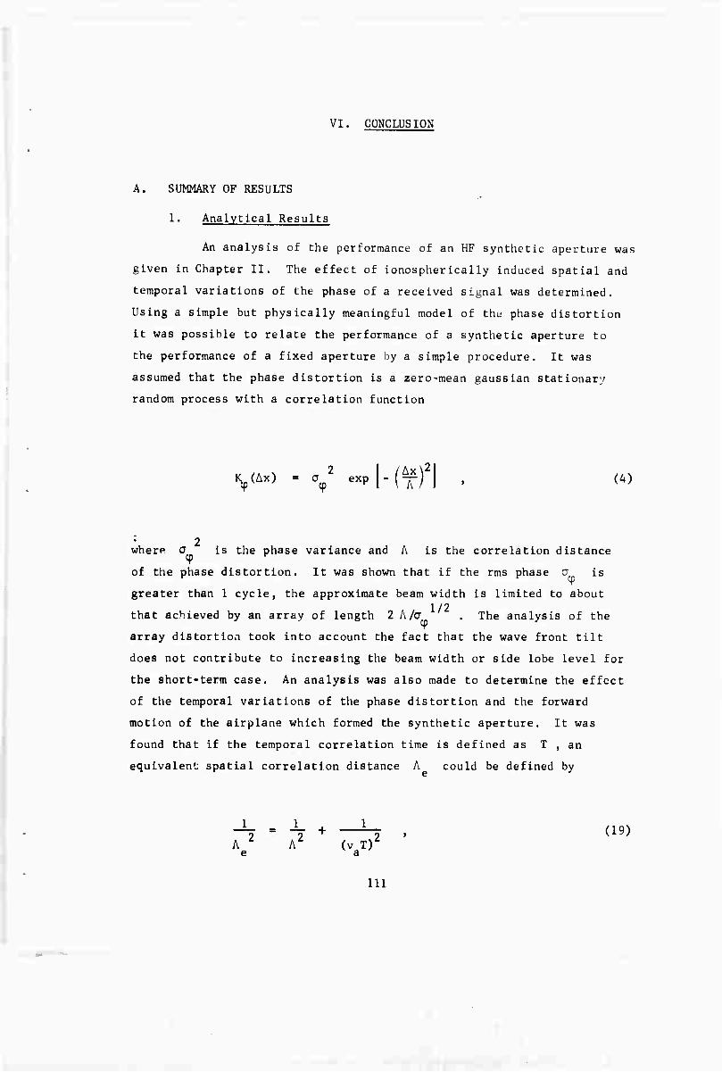
VI. CONCLUSION

A. SUMMARY OF RESULTS

1. Analytical Results

An analysis of the performance of an HF synthetic aperture was

given in Chapter II. The effect of ionospherically induced spatial and

temporal variations of the phase of a received signal was determined.

Using a simple but physically meaningful model of the phase distortion

it was possible to relate the performance of a synthetic aperture to

the performance of a fixed aperture by a simple procedure. It was

assumed that the phase distortion is a zero-mean gaussian stationary

random process with a correlation function

2 K (Ax) = a exp 9 «P m2\ . <*)

2 where a is the phase variance and A is the correlation distance

of the phase distortion. It was shown that if the rms phase a is

greater than 1 cycle, the approximate beam width is limited to about 1/2

that achieved by an array of length 2 A/a . The analysis of the

array distortion took into account the fact that the wave front tilt

does not contribute to increasing the beam width or side lobe level for

the short-term case. An analysis was also made to determine the effect

of the temporal variations of the phase distortion and the forward

motion of the airplane which formed the synthetic aperture. It was

found that if the temporal correlation time is defined as T , an

equivalent spatial correlation distance A could be defined by

J^ = J_ + —L^ > (19) A Z AZ (v T) e v a

111

■ „.

whe ri is the velocity of the airplane.

The quantity 1/A is proportional to the rms increase in beam

width (beam spreading). Therefore the above equation simply states that

the variances of the two causes of beam spreading (spatial and temporal

variations of the phase distortion) add.

In Chapter III an analysis was made of restoration techniques

for UF synthetic apertures. It was found that the optimum restoring

filter would compensate for amplitude and phase if the reference signal

and the Information bearing signal were distorted in exactly the same

way. As the point to be imaged moves further from the reference, the

distortions suffered by each become uncorrelated with one another, and

the optimum filter de-emphasizes the amplitude information. Whether a

practical spatially-invariant filter would utilize amplitude information

or not depends on the degree and type of distortion. It was found

analytically that the improvement in array performance afforded by a

phase reference could be determined by defining an equivalent phase 9

variance o ' by

2 a' 1 - exp ■m (36)

where Ay is the separation of the point to be imaged from the refer-

ence. Thus the problem of an array using a reference was reduced to the

previously solved problem of an array without a reference. In Chapter

III, Eq. (34), it was shown that a small amount of distortion would

occur if Ay was restricted by

Ay 2a,

■

112

where a« is the rms angle of arrival. Thus the size of the region

which can be imaged is inversely proportional to the rms angle of

arrival a. . For a wave length X = 20 m , and an rms angle of "o

arrival afi = 1/4 deg, the separation Ay should be less than 2.5 km. Oo

This is a stringent restriction.

2. Experimental Results

The experimental program was organized into 4 principal steps:

Verification of airplane-tracking subsystem performance.

Measurement of beam width achievable with the synthetic aperture when receiving a CW signal transmitted from Bearden (CW forward-propagation experiment). In this test, compensation for deviations of the airplane from a linear flight path was applied by the use of airplane tracking data.

Demonstration of the feasibility of obtaining two-dimensional backscatter data (range vs cross range) without compensating for iono- spheric distortion or deviations of the airplane from a linear flight path.

Investigation of the use of an HF repeater at Bearden to provide a reference signal in compensating for airplane flight-path deviations and ionospheric distortion, for the purpose of obtaining extremely high azimuthal resolution in backscatter mapping.

The experimental results were obtained using the F layer of

the ionosphere to propagate a one-hop signal. The particular path used

was an east-west midlatitude path which generally has favorable condi-

tions. The data were taken during a period of low magnetic activity,

and in general the ionosphere was undisturbed.

a. Airplane Tracking

The airplane tracking system proved to be quite accurate.

A comparison was made between locations determined by the radio tracking

113

&j&^iw.m^w-.:. ..■-«—■■

system and locations determined by photogrammetry at the ends of the

flight path (separated by about 60 km). On the lour flights tested the

location error was Less than bU m.

b. CW Forward-Fropagation Measurements

The frequency spectra of CW signals transmitted from

Beardun and received at either Los Banos or in the airplane were calcu-

lated by Fourier-transforming the data in time intervals of certain

lengths. The forward motion of the plane produces a synthetic aperture,

so that the frequency spectrum of the signal received in the plane is

equivalent to an angular spectrum. If is essential in these CW measure-

me'U s that the deviations of the airplane from a straight course be

Compensated for.

For the data received at the fixed receiver in Los Banos

it was found that processing times as long as 256 sec could be used to

obtain an Ü.OO-* Hz frequency resolution only a small fraction of the

time. Processing times of 128 sec could be used about 50 per cent of

the time, and processing times of 64 seconds about 80 per cent of the

time. By comparison, the signal received in the airplane could be

processed for 64 sec, giving a 5 km aperture, to yield an 0.008 Hz

frequency resolution (or equivalently a 1/b deg azlmuthal angular

resolution at 23 MHz) about 50 per cent of the time. It was found that

a synthetic aperture 10 km long could be used to form an azlmuthal beam

about 1/12 deg wide for about 20 per cent of the cases tested.

Thus it seemed that the spatial as well as the temporal

variations oi the ionosphere limited the resolution of the signal

received in the airplane.

c . Ikickscatter Measurements Made Without Compensation for Flight-Path Deviations or Ionospheric Variations

Baikscatter measurements were made by transmitting a

SFCW signal once per second from Lost Hills and receiving the backscat-

ter signal Ln the airplane. A fixed repeater at Bearden at a range of

2600 km, Which simulated a ground backscatter return, plus a natural

114

■»

backscatter enhancement at a range of 1600 km were imaged. It was found

possible to obtain a 0.4 deg beam width at 15.6 MHz using a 2.5 km

synthetic aperture.

d. Backscatter Measurements Us ins a Repeater Signal to Compensate for Flight-Path Deviations and Ionospheric Variations

In these studies, the fixed repeater at Bearden was used

not only to simulate a large ground backscatter return, but also to

furnish a reference signal for use in compensating for airplane flight-

path deviations and ionospherically induced distortions. In addition,

a portable repeater was installed at Bearden at a site 1000 m north of

the transmitting site of the fixed repeater. The portable repeater was

used to simulate a large backscatter return and thus to determine the

effectiveness of the compensation system in permitting high-resolution

discrimination by the synthetic aperture as between signals from the two

simulated backscatter sources.

The major test employed a synthetic aperture which was

70 km long and required about 13 minutes to form. Using only the phase

information from the fixed repeater to implement the compensation, the

beam width obtained was about 0.02 deg, which is larger by a factor of

two than it would be in an ideal case. However, using amplitude and

phase Information from the repeater, a beam width of 0.01 deg was

achieved, as shown in Fig. 32. The cross resolution of the 0.01 deg beam

was about 470 m. Thus the fixed repeater and the portable repeater were

resolvable in cross range (azimuth). However, the cross-range side lobes

of the portable repeater signal were much higher than they would be in

an ideal distortionless case. Since the distortion increases rapidly as

the point to be imaged moves further from the reference, it is not ex-

pected that a point more than 3 to 5 km from the reference could be

imaged without distortion.

B. CONCLUSIONS

There are three possible methods of operation of an HF synthetic

115

2 .

^P^^BIPI^PPP||||P|IB|>^pWBWIlllH-i|li.liLi«iimHH. n.M..uy.iiiu. ■..iii.nii L. .1.1 ,i n in

aperture which hav« bean developed and for which separate although

related conclutlom are drawn. Theaa methods are:

1. Operation wi thout compensation fur airplane flight-path deviatlona from a straight line or lor Ionospheric distortion.

2. Operation with compensation for flight-path deviations by means of an airplane tracking system, but not for ionospheric distortion.

3. Operation using an HF repeater to provide a relerence signal Lu compensate for both flight-path deviations and Ionospheric d istort ion.

1, No Compensat ion

In the ClrMt type of operation, for which no compensation of

any kind was used, it was found experimentally that a synthetic aperture

3 km long could be used to form an azimuthal beam about 0.4 deg In width

(at 23 MHz). This was achieved about 50 per cent of the time. The

result was verified using both the CW forward-propagation measurements

and the backseatter measurements. One of the Important parameters of

these tests was the type of aircraft used to synthesize the aperture.

In ehe tcsu: reported here a medium sized airplane, a twin-engine DC-3,

was used for the test. The airplane flew at a speed of about 80 m/sec

(180 miles per hr). Deviations of the course of the plane from a

straight lint appear to be the limiting factor in the system performance

even with the aid of a trained navigator, and even when detailed ground

maps and a telescope are used to determine with great precision the

location of the plane. The 2.5 km aperture that was successfully syn-

thesized without any compensation is comparable In length with the phased

array operated by the Stanford Radlosclence Laboratory flt Los Banos,

which is believed to be the world's longest HF array.

2. Flittht-Path Compensation

In the second method of opeiatlon, in which airplane deviations

were compensated for, it was found that an aperture 10 km long could be

116

-_ — ■ — «■■iljiijilPMiliiiiiijiiiiiLJ.yiiw.immpiiwipii

used about 20 per cent of the time to form an azimuthal beam of

approximately HV. deg (at 23 MHz). This was verified uslnfe the CW

forward-propagation measurements. Measurements were made of the same

CW signal as received In the aircraft and as received at a fixed antenna

at Los Banos. A comparison of results obtained for the fixed and the

airborne measurements indicated that spatial and temporal variations of

the phase distortion were limiting the performance of the synthetic

aperture. Apparently, better results could be obtained by flying faster.

A fixed aperture, which Is the theoretical equivalent of an infinite-

flying speed, should be able to perform even better than the experiment-

ally realized synthetic aperture. A fixed aperture of 10 km in length

should be able to achieve narrow beam widths without significant

distortion a large fraction of the time.

3. Flight-Path and Ionospheric Compensation

In the third method of operation. In which an HF repeater was

used to compensate for flight-path deviations and ionospheric distor-

tion, It was found experimentally that much increased azimuthal resolu-

tion could be achieved In the region near the reference. A 70 km syn-

thetic aperture was able to obtain a cross-range resolution of about

500 m at a range of 2600 km. A second repeater 1000 m away which was

used to verify the cross-range resolution appeared to have very large

side lobes. Since the improvement In performance afforded by the refer-

ence signal diminishes rapidly as the distance between the point to be

Imaged and the reference increases. It Is expected that the region which

can be Imaged Is less than 3 to 5 km.

One Is forced to conclude, therefore, that the use of a

reference signal can Indeed make it possible to obtain extremely high

cross-range (azimuthal) resolution, but that this resolution can be

achieved only In a region vary close to the reference point.

4. Overall Conclusions

The investigation reported here clearly shows

that aperture synthesis techniques can be used for

117

■

WW|IBWW»PPiig»™iBp||pip|Pi^iwwiiiiLJjjJtuji_.tJ^i.i!.iu.jLijLtjij LI

signals propagated via Liu- F layer ot tla- tonosphere. The principal

advantages ot using aperlure synthesis are (I) that the receiving

equipment Is by Us very nature portable, and (2) that apertures much

longer than any ever built for use at HF are easily Implemented. The

analytical and experimental program have helped to delineate the

fundamental limitations In Implementing aperture synthesis at HF.

It should be noted that the conclusions which are drawn from

the experimental program are for a particular set of Ionospheric condi-

tions which are generally regarded as quite favorable. These conditions

Included a mldlatltude east-west path which Is known from other studies

to have favorable properties such as small pulse spreading due to

magnetolonic splitting, and small azlmuthal spreading. The data were

taken during a period of low magnetic activity and In general the Iono-

sphere was undisturbed. Another Important qualification Is that only

one-hop F-layer propagation was tried. Presumably mu!tl-hop signals

would sustain severe distortion because of the Intermediate ground

reflection, which would make aperture synthesis difficult. On the

other hand, one-hop E-layer propagation might have produced far superior

results; however, this mode Is not available for the 2600 km path used

In this study.

Under the conditions outlined above, It has been shown

experimentally, that the use of suitable compensation for ionospheric

distortion, employing a reference signal close to the backscatter-Imaged

area, permits extremely high azimuth resolution with synthetic apertures

on the order of 70 km In length. This technique has two significant

disadvantages, however. Firs.., high azlmuHial resolution can be

achieved only in a very small region surrounding the reference, about

± 3 km in extent. Second, It may be Impractical to provide such a

reference near the region to be imaged. Based on the analysis presented

herein, these same restrictions apply to extremely long fixed apertures

as wel1.

It lb concluded that aperture-synthesis techniques are

particularly attractive for apertures of between 1 and 10 km In length.

For the shorter apertures, 1 to 3 km, It should be possible to jbtaln

118

■. .

-—' ,— wmmmmmm*"" ■ ■■■—■ ■ '

full benefit of the aperture by using a medium-sized airplane and simple

processing techniques which would not compensate for course deviations

of the plane from a straight line. Longer apertures, 6 to 10 km, could

be used effectively at least part of the time, if compensation for

course variations over a time interval of 60 to 100 seconds could be

provided.

C. RECOMMENDATIONS FOR FUTURE WORK

The research that has been described herein leads to the following

suggestions for further study in the field.

1. Other Forms of Compensation

If temporal variations in the ionosphere are the limiting

source of error, a compensation for only these variations could be used.

The phase of the transmitted SFCW signal could be modified in accordance

with changes measured from a single-mode, one hop CW signal propagated

over the same path. The source of the CW signal would have to be phase-

stable, and the signal would have to be propagated by only a single

mode. The use of the National Bureau of Standards broadcasts of fre-

quency standards on Station WWV, Colorado, might be useful in certain

regions.

A slightly more complicated version of the same idea is to

receive at the transmitter site and in the airplane a CW signal trans-

mitted from a point near the region to be imaged. The phase of the

received CW signal could be usod to compensate both the transmissions

and the SFCW backscatter in real time as it is recorded in the plane.

Thus both the transmit and the receive paths would be compensated. The

processing involved Is a two-dimensional Fourier transform, since both

geometrical effects and flight-path variations are accounted for. The

use of CW transmitters as references rather than broadband repeaters is

appealing from a practical standpoint. With CW transmitters, the use of

multiple reference signals becomes much more feasible than with a single

reference. This would extend the region that can be compensated. (See 30 Goodman and Gaskill for a discussion of multiple references for

119

fmmu ■."mmmmmmmi» ' -~ '—■ •' ■■'——"■:—■ ■— "

holography.) With multiple references it should also be possible to

account for changing ionospheric tilts, which would greatly extend the

region that tv>uld be mapped. For example, with two referunces It should

be possible to measure not only the phase but also the slope (rate of

change In spate) of the phase.

2. Use ol Faster and More Stable Airplanes

A small Jet airplane with a high wing loading ratio (gross

weight/wing area) could fly at speeds of over 700 ml/hr, which is about

four times the speed of the DC-3 used In the experiment, and would be

much more Immune to the effects of atmospheric turbulence and winds. A

radio or Inert la I navigation system might also be used to measure the

flight path and compensate the data In real time as it is recorded.

Even without the navigation system, the more stable plane might be able

to syiithesize apertures as long as 23 km without the necessity for

flight-path compensation of the data.

3. Use of Optical Prort-ssing vs Airborne Computer Processing

The scope of the present project did not warrant the use of

optical data-processing techniques because of the complication this

would introduce. Furthermore, the digital processing of data rprmltted

considerable flexibility in rompensating for geometrical effects and

flight path variations. However, other means of compensation might be

possible which would make the two-dimensional Fourier-transforming

properties of optical lenses usable. This would be ideal for processing

large quantities of data. The possibility of using a medJam-sized

general purpose computer instead of optical processing should not be

overlooked, however, since the cost of optical equipment may be compar-

able with that of the computer. If costs are comparable, the possibility

of making real-time images with the computer becomes attractive. The

computer could be airborne, or the data could be relayed via a radio

link.

120

i,. ._ . . _ ____ __ -- - -

wmmmi

4. Use of Longer Synthetic Apertures. Wider Band Widths. Higher Frequencies, ami Shorter Ranges

By using a 200 km synthetic aperture, a 20 MHz center

frequency, and a 5 MHz band width, a resolution of 0.2 minute of arc -5

(5 x 10 radian) and 200 nanoseconds could be attained, at least

theoretically. At a range of 1000 km the resolution cell on the ground

would be rougMy 50 m by 50 m. The use of such a large aperture and

band width would definitely require very careful compensation. Antennas

which arc circularly polarized and which therefore excite only one

magnetolonlc mode would be extremely beneficial. The mathematical

analysis of HF synthetic apertures indicates that the size of the region

around the reference which can be successfully imaged depended on the

correlation distance and the rms phase perturbations, but not in a

direct way on the size of the- aperture. Even if the region which could

be Imaged were only -t 3 km in extent, a map with 120 by 120 resolution

cells could be made.

5. Use of Incoherent Processing Techniques

Incoherent processing for the purpose of measuring the angular

distribution of received energy refers to a technique which does not

require a high degree of phase stability in the received signal. There

are two principal types of Incoherent processing.

The first type is analogous to conventional optical imaging.

It Is used In radio astronomy to measure the location and size of radio

stars. The basic principle Is to measure the average amplitude and

phase of the product of two signals received at two points. The Fourier

transform of this average amplitude and phase vs receiver separation

yields the angular energy distribution of the Incident incoherent signal.

The key to the process lies In the averaging. An incoherent technique

for an HF synthetic aperture has been proposed by Shearman. Although

Shearman uses coherent transmissions to obtain backscatter energy, he

averages ehe data over long periods of time, and assumes that the iono-

sphere introduces the necessary signal Incoherence to make the processing

work. The long average such as an hour might be required for each

121

.. . . _ .__.___ . ... ._ *

IM, IWIiillRW^lWI^Wliuiiiiinwii "" ———ii .1.. w m mmmmmmm***!««™»'"»'^''**

•paclngj there tore In the Shearman method a modest map with only 100

elemencs could possibly take days to measure.

The second type of Incoherent processing usos the delay

resolution of the signal. It therefore discards i-adlo frequency phase

at the outset (after delay resolution Is obtained), by using envelope

detection. The basic principle Is that the angle of arrival of the

signal dftermines the relative time of arrival on Individually spaced

receivers. The accuracy of the method depends on the pulse width (I.e.,

the signal band width) and on thl separation of the receivers. (Con-

ventional phase processing depends on the wave length and thus on the

frequency.) The Incoherent processing would have an accura^v much

poorer than the coherent processing by a factor equal to the ratio of

the signal hand width to the center frequency. While the performance

Is thus much worse, the system design for Incoherent processing Is In

principle much easier, since the phas<.> of the signals does not have to

be preserved. Thus It becomes feasible to use receiver separations of

tens of miles. The use of the second type of Incoherent processing may

be well suited for direction finding (DF) but appears to have many

severe disadvantages for Imaging. The major problem is that it would

appear to be sensitive only to very large changes In the reflectivity of

the surface that it was imaging. This would be similar to the self noise

problem discussed in Chapter III except much more severe.

The use of multiplicative processing whereby the outputs of

antenna elements are correlated with each other also has application to

the situation where there are only a few points to be imaged. Cross-

product terms Inherent in the nonlinear process would make the applica-

tion to imaging Inappropriate.

6. Use of Other Ionospheric Modes and Conditions

The distance the HF signal propagates corld affect its

coherence properties. The longer the signal path the less deep inf) the

ionosphere the ray tends to go. The experiment reported here used a

midlatitude east-west signal propagation path, which provides very

favorable ionospheric conditions. A path differently oriented might

122

■ w. ■■

F—' ■■■"■" -H- J"11 ' ' —~— _

encounter effects of the auroral or equatorial zones. The high

Icnospherlc activity of these zones, especially the auroral zone during

or following solar disturbances, would certainly limit the performance

of any HF aperture. From the opposite point of view, however, the sen-

sitivity of HF signals to the Ionospheric variations and the highly

portable character of the synthetic aperture make the latter an attrac-

tive means of studying large-scale disturbances in these normally hard-

to-reach areas of the globe.

Meteors and sporadic E can distort Ionospheric signals and

therefore would affect synthetic-aperture performance. Should meteors

prove to be Important at certain HF frequencies care could be taken to

operate only at periods of low meteoric activity, such as the evening

hours. The presence of sporadic C Is readily detectable on

oblique lonograms and could therefore be avoided by selection of a

suitable operating frequency If It also proved to be a problem.

The use of the E layer for Ionospheric propagation could offer

significant Improvement in performance. One-hop E can generally propa-

gate up to distances of 1500 km, which Is sufficient for many applica-

tions. The E layer Is known for Its exceptional temporal stability,

which suggests that It may preserve the spatial phase coherence of HF

signals as well. The Importance of further large-aperture experiments

designed to utilize the one-hop E mode cannot be over-emphasized.

7. Applications to Direction Finding (DF)

Thus far the synthetic-aperture technique has been described

as a way of improving the quality of backscatter records. As pointed

out In the Introduction, the main attraction of HF synthetic apertures

Is the elimination of the huge size of physical structures otherwise

required to achieve narrow beam widths. At frequencies In the 2 to 3

MHz range, the argument Is even more compelling. Yet this Is the fre-

quency range of the radio equipment carried by many small ships. This

frequency range propagates via the E layer In most circumstances, both

day and night. The Coast Guard or other sea-rescue organizations might

find the synthetic-aperture technique extremely helpful In their mission

123

■

'■-■-■ ■• ■ '■ ■ ■ l■■ ' ■■um»««! H!liliiujiiiim HU. Mil» .1 .m I.III.»IIPWIP»W<PIIP«'^IIIII..IIII.IWIPWIWI|UI'II

of lucatlnK ships In ilihlrosu.

In view ut tht abovu consIderations, the possibility of using

the synthetic aperture to measure the direction of arrival of unknown

signals will now be Jiscuised. Direction finding (OF) is a major

problem in many situations such as sea rescue. A downed plane or a

disabled ship may be able to transmit a CW signal on some emergency

band. A relatively short synthetic aperture, about 1000 m long, would

be able to obtain high precision without the usual site errors caused

by the large metal structures of ship-mounted OF systems. An aperture

of about a 1000 m would requite only about 10 seconds to fly. Thus the

stability requirement on the unknown transmission wou'd be very low,

and would be satisfied by almost all unmodulated signals.

Since only modest apertures are required, the synthetic

aperture for land-based operations could be implemented in a truck. At

highway speeds (65 mi/hr), a 10 sec integration time would give about

a 300 m aperture. Thus the portability of the truck would make it

possible to synthesize an array whose performance would compare favorably

with that of a fixed array the length of three football fields. Of

course, the availability of suitably oriented, reasonably straight roads

might limit the size of the aperture achievable by a truck to a more

modest size.

124

■

^_ .

■ — '■— ' "■■" "■'- '■

Appendix A

DESCRIPTION OF EQUIPMENT COMPONENTS

A. BACKSCATTER-SIGNAL TRANSMITTER AT LOST HILLS

The backscatter-slgnal transmitter consUted of a cesium-beam

clock, a swept frequency CW generator, three 10 kW power amplifiers,

and a narrow-beam antenna array.

The cesium-beam clock was a portable time and frequency standard

(Hewlett Packard S061A) of exceptional short- and long-term stability.

Three of these clocks were used in the experiment (transmitter, airborne

receiver, CW tracking transmitter). The long-term stability Is less

than one part In 10 . The outputs of the clock Include: one pulse

once per second with a 50 nsec rise time; a 100 kHz sine wave; a 1.0

MHz sine wave; end a 24-hour clock face with a second hand which moves

incrementally once per second. This last feature is extermely useful

In synchronizing start times at the distant sites.

The SFCW generator was a Barry Research LSG-6, which has flexible

sweep rates and flexible start and stop frequencies. The output was

swept at a 1 MHz/sec rate, once every second, across a 600 kHz band.

The start time of each sweep Is determined Liy a one-pulse-per-second

(1 pps) signal from the cesium-beam standard. All signals in the

generator are derived from a 1 MHz sine wave, which is also from the

cesium-beam standard. A description of the principles of operation of 31

the generator has been written by Fenwick and Barry.

It Is essential chat the SFCW signal be exactly the same from sweep

to sweep. In particular, the phase of the signal must be the same. The

SFCW units did not meet this requirement for all possible sweep rates

and starting and ending frequencies. However, the requirement was met

for the 1 MHz/sec and 250 kHz/sec sweep rates when the starting fre-

quencies are an Integral multiple of 100 kHz.

The power amplifiers were Collins 208 U-IO transmitters, with an

auto-tuning feature. Because of the fast sweep rate used, and the

relatively narrow band swept, the units were operated on a fixed tuning

125

_ _._ . *. .

"—

basis. Al tor stagBt-r-Uinlug the output section, the i dB band width

of the transmitters was about 400 kHz. There was therefore some ampli-

tude variation in the output signal. The variation was symmetrical, so

that its el feet on the final processed signal was to reduce range side

lobes.

The three amplifiers fed an IB-element array. The elements were

ITT Folded Tilted Monopoles (t'TM) with 12 m spacing, giving a total

aperture of about 204 ra. A reflector screen provided unidirectional

radiation eastward. Although the array Is capable of beam steering, it

was operated in the direction of Bearden, Arkansas (see Fig. 13). The

three amplifiers fed the 18 elements in a symmetrical power taper in

order to reduce the angular side lobes of the array.

B. AIRPLANE

A twin engine, medium sized airplane (DC-3) was fitted with two

tubular antennas and a gasoline generator for ac power. The plane had

to be large enough to hold several racks of equipment, a large aerial

camera, and six people including two pilots. Heavy weight was desirable

to reduce the effect of short-time wind fluctuations, since the plane

should fly a straight course. A fast aircraft was desirable to reduce

the effect of temporal variation of the ionosphere. The DC-3 was

reasonably priced for rental ($195/hr), met all of the requirements

except speed, and was available. Its speed was about 180 miles/hr

(80 m/sec), which means It required about 20 minutes to fly the

prescribed flight path (i.e., to implement the synthetic aperture).

Only a limited amount of 100 V 400 Hi power was available in the

airplane. Therefore, in order to provide power to the electronic equip-

ment, a small gasoline generator was Installed in the tail section of

the plane. Precautions approved by the FAA were taken to reduce fire

hazard. The generator provided 2 kW of 120 V power at (60 ± 1) Hz. An

averaslng electromechanical voltage stabilizer was used, which did not

introduce distortion in the 60 Hz signal.

The plane was ground- and flight-tested to determine if aircraft-

generated radio noise was a problem. After a faulty generator was

126

■

■PiC^'^

replaced, the aircraft-generated radio noise was less than the ambient

radio noise. The use of additional static precipitatord was found not

to be necessary, due perhaps to the prevailing dry weather conditions.

The two HF antennas installed on the airplane for the experiment

consisted of 12 ft lengths of Ik in. aluminum tubing. One cf these

tubular antennas was mounted vertically near the vertical stabilizer;

the other antenna was extended horizontally from the tail. Figure 33

is a photograph of the airplane exterior showing the antennas. A ground

test at 20 MHz wiLh a field strength meter at a radius of 150 ft re-

vealed that the vertical stabilizer of the airplane did not appreciably

affect the vertical pipe antenna, although the engine mounts and the

forward section of the fusalage did. A bandpass filter (20-26 MHz) and

an Impedance matching network (VSWR about 2:1) were used. Because of

the strong Influence of the metal airplane body. It was not expected

that the vertical and horizontal pipe antennas would be orthogonally

polarized. It was expected only that the two antennas wculd be

differently polarized. This was In fact demonstrated to be the case In

tests conducted during flight. This circumstance made It possible to

determine If signal-amplitude variations were due to polarization

effects.

Braodbanding the antennas on the airplane proved difficult.

Several configurations of the common wire-type antennas were tested,

but proved unsatisfactory. The tubular antennas were Impedance-matched

over the 20-26 MHz band without difficulty In a test setup, but proved

to be a problem when mounted on the airplane. Trlal-and-error adjust-

ments of the Impedance matching network finally gave a VSWR within 2:1

from 21:1 to 25.7 MHz.

The electronic equipment was strapped securely on foam rubber pads

with nylon bands secured to the aircraft frame to reduce vibration and

minimize the hazard of equipment breaking loose In flight.

C. AIRBORNE RECEIVING EQUIPMENT

The airborne receiving equipment Included a cesium-beam clock, an

HF receiver, and an SFCW generator. A simplified block diagram showing

127

■

^_ r

Figure 33 Airplane used in synthetic aperture experiment, showing horizontal and vertical tubular antennas.

128

.

their relationship is shown in Fig. 34. The clock and the generator

were exactly the same as the clock and generator used at the transmitter,

The SFCW generator was also swept at a one MHz rate, once per second.

Its start and stop frequencies were set 18 MHz higher than those of the

transmitted signal. Demodulation occurred when the received signal and

the local SFCW were mixed on a hot-carrier-diode balanced-mixer. The

difference frequency of 18 MHz was selected by the receiver.

The receiver was a Collins 75S-3. Its internal injection

oscillators were disconnected, and in their place injection signals were

synthesized by i;he LSG-6 driver unit which uses the 1 MHz signal from

the cesium-beam clock. The receiver band width of 6 kHz was determined

by a mechanical filter in the IF (intermediate frequency) section. The

output signal was close to 1 V peak-to-peak (p-p) in the band 2 to 8 kHa.

The dynamic range of the receiver was about 40 dB. The receiver was

linear over this range.

A detailed block diagram of the airborne receiving equipment is

shown in Fig. 35

The time of the 1 pps signal of the clock is digitally adjustable

by a precise amount. This adjustment, known as setting the clock delay,

has the effect of changing the final output frequency of the backscat-

tered signals. In the experiment the demodulated output signal due to

the repeater at Bearden was set to be at 4 kHz. This frequency chosen

so that the desired backscatter ranges would fall within the 6 kHz

pass band of the receiver and make the sampling operation more

convenient.

D. AIRPLANE-TRACKING SUBSYSTEM

The airplane-tracking subsystem included two ground fixations for

transmitting CW signals; receiving equipment in the plane; and a

digital computer (XDS Sigma 5) for off-line processing of the recorded

data. The CW signals were in the 20 to 26 MHz band in order to use

available antennas and transmitters and receivers. One transmitter,

located at Los Banos, was in a van which housed the processing equip-

ment for the Stanford 2.5 km HF array. As shown previously in Fig. 13,

129

-....--..--

— 1

I TRACKING RECEIVER

CESIUM-BEAM FREQUENCY STANDARD

w VERTICAL ANTENNA

1 RECEIVER

No. 1

TO LOCAL OSCILLATORS

SFCW GENERATOR

AND SYNTHESIZER

Ü 1 PPS-

50 kHz-

ALTIMETER

V HORIZONTAL

ANTENNA

M U

ANALOG TAPE

RECORDER

Figure 34 Simplified block diagram of receiving equipment.

130

^■-'•-~ ■ ■ , ■.-,:■

i 1 ■J

r

< z y z

> < t>^i

<^

o ̂ z cc I 6 1- ^ < Ul s z

z o p UJ

e

-#-

z o 1- u

o o 8 z ^^ ■o c <N

o 1-

cc o

» 1- M <

c UJ >

W UJ oc z a UJ u

^^^^

N z 5

(E in UJ f) u. 3 ^— a. S <

o u. ca. O

OC (3 rr UJ Z Ul N

(J > Üj M UJ Z )- < U

1- z

c 0) e Q. '5 o- 0)

Ol c ■>

'53 ä

E S (0

I T5

"I

S 0)

e

131

■

.._.. .. _... . _ _ . . _ _ _

this Los Banos site is sitrated so that the flight path if extended

would pass over It Tims this signal could be processed to give the

position of the plane along the flight path, and also could be used as

a real-time precision speed indicator. The Los Banos site is line-of-

sight to the plane if the latter is on the flight path at an altitude

of 60Ü0 ft. The site was furnished with a cesium-beam clock which was

required to guarantee that phase variations in the transmitted signal

would not be responsible Cor more than 5 m of error in the coordinates

of the plane. A Johnson Viking II transmitter with close to 100 W

output, and an HP frequency synthesizer (5100 A) were used to generate

the CW s igna I.

The second transmitter was located at a point near the perpendicular

bisector of the flight path. This site was at the FAA VHF radio facility

on Bear Mountain near Copperopolis , Calif, at an altitude of 2893 ft.

The site was selected to be line-of-sight to Los Banos and the entire

flight path, which is a difficult selection owing to the many inacces-

sible areas in the Sierra foothills. The Bear Mountain site also used

a Johnson Viking II transmitter and a Manson Frequency Synthesizer with

an internal crystal standard to transmit a CW signal 3 kHz higher than

the signal from Los Banos. To make the average signal strengths of both

transmissions approximately the same over the flight path, the Bear

Mountain transmitter was operated below 100 W. A 13 ft vertical whip

with two 30 ft radials was used at this location.

The frequency band used (20-26 MHz) is well above the critical

frequency of the ionosphere and therefore vertical ionospheric reflec-

tion is not likely. It is possible for a ground-reflected path between

the ground transmitter and the airborne receiver to interfere with the

desired 1ine-of-sight path. This interference is readily detectable as

amplitude modulation on the received signal. Fortunately, this inter-

ference was not observed during most of the experiment. The lack of

such interference is attributed to the low gain of r.he Bear Mountain

transmitting antenna at elevation angles close to ziro degrees. It is

also possible that the vertically polarized wave and the low ground-

reflection angles make the ground reflected signal small. A more likely

132

A ' '^ ■ ^ u- "*

■" '— " .I-.. ■wjm.m.i. .

problem is that the omnidirectional antenna would propagate a wave

backward which could be reflected by the High Sierra. Such a reflection

would be aspect-sensitive, and therefore the interference would vary

greatly with the plane's position. In fact, amplitude fluctuations

were observed on occasion at the north end of the flight pa.h.

The crystal standard at the Bear Mout.tdin site had a stability on g

the order of one part in 10 , which is three orders of magnitude less

than required. Rather than using another cesium-beam clock, the problem

was solved by receiving the Bear Mountain signal at Los Banos. The

received signal from Bear Mountain and the locally generated signal

were recorded using the same scheme as used in the plane. The analog

tape was later processed with the airplane tapes on the Sigma 5 computer;

the instability of the Bear Mountain crystal standard is therefore

compensated in the digital processing.

The receiver in the aircraft was a Collins 75S-3 with the same

modification for external coherent frequency conversion injections as

the receivers used for the SFCW data. The 6 kHz pass band made it

possible to receive both CW transmi&sions simultaneously, since they

were only separated by 3 kHz. The receiver output consisted of CW

tones at 3 and 6 kHz, which were recorded.

The 3 kHz Los Banos tone was also used to measure ground speed in

real-time with extremely high precision. The average period of 1000

cycles of the 3 kHz was measured continuously by an HP 5245L frequency

counter. The measurement was made with a 1 MHz reference; thus the

precision was 1 M-sec for the 333 msec interval of the 1000 cycles. A

three digit HP 5280A digital-to-analog converter was employed to obtain

a meter reading using the three least significant digits. The measured

period was inversely proportional to ground speed; but since only small

variations in speed occurred, the indicated meter reading was essen-

tially proportional to ground speed (with a change in sign). A full-

scale reading was approximately 4 m/sec or 5 per cent of the nominal

ground speed. In practice it was found possible to hold the ground

speed to about ± 1.5 m/sec.

A sensitive aneroid altimeter made and donated by Rosemont

133

IP!" 11 • 11 w^***^

Engineering Company was used which had a full-scale reading of ± 40 m.

The meter had a zero adjustment, so that when a desired altitude was

attained the meter could be used by the pilot to maintain that altitude

(utiually at ± 10 in). A dc signal proportional to the meter reading was

recorded for later use in the off-line computer tracking program. The

meter had an error due to hysteresis which was less than 3 m. To

account for variations in the ambient air pressure, temperature-cor-

rected barometric readings were obtained from the Sacramento and

Stockton, weather bureaus. For most flights, this correction was less

than an equivalent of 10 m of altitude and was therefore not used in

the tracking program for these very stable cases. Both ground-speed

and altimeter readings were provided by remote meters in the cockpit.

The CW signals permit the measuretr.nt of changes in the distance

to the two CW transmitters at Los Banos and Bear Mountain, respectively.

This Information can be accurately translated into the plane's position

coordinates only if the coordinates of the starting point are known

accurately. The latter measurement is made by taking a stereoscopic

pair of aerial photographs of a ground marker using photogrammetry

techniques. A ground marker was accurately positioned at each end of

the flight path by an aerial survey firm. One marker was near the new

Sacramento fair grounds, the other near Manteca (see map, Fig. 15). The

error In the measurement was specified to be less than ± 50 m on the

horizontal, and ± 100 m in altitude. Using one marker as the starting

point, the other marker can be used to test the accuracy of the tracking

data. On four flights the error was between 20 and 60 meters; consider-

ing that the two markers were separated by about 60 km, this result

represents a high degree of accuracy.

E. AIRBORNE ANALOG TAPE RECORDER

An HP 3917B 7-track analog tape recorder was used in the plane.

The half-inch tape ran at 30 in./sec (ips) to reduce inter-channel

timing jitter and to give the necessary band width to record a 50 kHz

reference signal. Extra long reels of tape (4600 ft) were used to make

the data cover as long a time interval as possible. Even so, the 30 min

134

■ _

1

duration of the tape was barely adequate to cover the distance between

the two ground marKers if a moderate head wind was encountered. The

inter-channel timing jitter is specified by the manufacturer to be less

than 1.0 P-sec which causes a 2 deg phase jitter in a 5 kHz CW signal.

While this phase jitter is not negligible, it was judged quite tolerable

for the tests being made.

The 50 kHz reference signal derived from the cesium beam standard

was used to synchronize the sampling signal during the A/D conversion

process In this way tape speed variations were compensated for, and

only inter-channel variations were a source of phase errors.

The tape recorder channel assignments and recording method are

given in Table 4.

TABLE 4

TAPE RECORDER CHANNELS

j Channel # Method Signal j

1 direct CW tracking

2 FM voice (experiment log)

! 3 direct 1 PPS

4 FM altimeter

5 direct 50 kHz reference

6 direct horizontal SFCW

7 direct vertical SFCW

The recorded signals were about 40 dB above internal tape recorder

noise, if the input signal level was adjusted properly. Thus noise from

the recorder was not significant.

F. HF REPEATERS

Two HF repeaters were used in the experiment. The principal

135

r*-

repeater is tixed in Bearden, Arkansas. It consists of two Collins

Log-Period Antennas (LPA's) which are horizontally polarized; a 2 MHz

bandpass filter; and a Marconi H'rOO-1000-02 1000 W broad-band amplifier.

The receiving antenna is located 1000 m north of the transmitting

antenna. The antennas are oriented to point their beam west, and to

have a minimum mutual coupling. This repeater Introduces about a S^sec

delay in the signal.

The second repeater was portable, and used a single antenna--a

12 ft whip. The repeater Is switched rapidly between transmitting and

receiving modes. The signal Is amplified, then stored In a delay line

for the duration of the receive perlud. At the end of that period It

Is transmitted. The keying Introduces frequency components not In the

received signal; however, for the SFCW signal used In the experiments,

these frequencies He outside the receiver p.assband. The delay line

was 63 (isec, which placed the side bands about 16 kHz away from the

repeated signal. The delay difference in the two repeaters is there-

fore about 58 Misec. A report describing the portable repeater Is 32

available.

For best results in the synthetic aperture experiment, both

repeaters should have a linear phase-vs-frequency characteristic, and

a phase which does not vary with time. Over a 1 MHz band width they

satisfy this requirement. Multiple echoes due to impedance mismatch

appear to be more than 40 dB down from the main signal. The largest

phase change with time was expected to be caused by the 1000 m above-

ground cable run, which connects the receiving and transmitting sites

of the fixed repeater. Measurements at the site indicate that the

fixed repeater Is phase stable. The portable repeater Is less

susceptible to temperature fluctuations and Is also phase stable.

The portable repeater was operated at several locations near

Bearden.

On various occasions the portable repeater was operated at the

receiving site for the fixed repeater; at the Naval Reserve Center in

Hiurell Field, about 17 km southwest of Bearden; at a cemetery a few

miles from Bearden; and In Sheridan, about 40 miles north of Bearden.

136

■

:

—

When the portable repeater was situated at the receiving site of

the fixed repeater, both repeaters shared the Collins LPA. The cable

to the transmitter site was connected to the switch In rwe portable re-

peater so that the fixed repeater and the portable repeater were keyed

on and off with a 63 y,sec period. Both repeaters received simultaneously,

The LPA has considerably more gain than the whip normally used on the

portable repeater.

G. CW FORWARD PROPAGATION SUBSYSTEM

The CW forward propagation subsystem used a crystal frequency

standard, a 1000 W linear amplifier and a vertical monopole antenna at

Bearden, Arkansas. The receiving equipment In the plane was exactly

the same as for the backscatter experiment except that the SFCW genera-

tors were operated in a mode where they provided a CW signal used for

the first frequency conversion external to the receivers. A receiver

was provided at Los Banos also which used one of the whips from the

2.5 km phased array there. The output of this receiver was recorded on

magnetic tape in exactly the same fashion as the output of the airborne

receivers.

H. OPERATIONAL PROBLEMS

1. Communications

It was necessf.ry for the plane, the Bear Mountain site, and

the Los Banos site to be connected by some form of communication.

Available VHP radio equipment was used between the plane and Bear

Mountain site; and a commercial telephone was used between Bear Mountain

and Los Banos. The standard V1T transmitter and receiver normally used

in the plane had adequate power (10 W) to provide usable communication

to Bear Mountain over the entire flight path, but not to Los Banos. The

use of Bear Mountain as a message relay point was decided on in order to

avoid installing new radio equipment. This was satisfactory for routine

messages, but for debugging the experiment it proved to be a handicap.

An intercom in the plane was also provided. The co-pllot and

137

■

■ '

navigator had a direct line as did the three SEL staff members.

Interconnection of the two direct lines could be made manually by the

flight coordinator (one of the SEL staff). The high acoustic noise

level of the plaiif made both shouting and the Intercom only partially

successful. (On several occasions, hand signals were the only recourse.)

Even though special acoustic noise reducing microphones were used, a

much more satisfactory solution could have been found with more time and

money. The Lntercotn communications and a tone marker actuated by the

camera shutter were recorded on the tape recorder.

A major drawback of the VHF communication link was that only

FAA authorized frequencies were used. These frequencies had to be

shared with others whic1- made long conversations difficult. (One day

flocks of Civil Air Patrol planes were searching for a downed plane;

on that day voice transmissions were limited to occasional 13 sec

bursts.)

2. Local Weather Limitations

Ideal conditions were clear skies, no wind, and plentiful

light. These rarely occur. The most Important condition Is no clouds

up to 6000 ft, the nominal altitude of the plane. Cloud cover beneath

the plane makes It Impossible for the navigator to maintain a straight

course, although he did remarkably well If the ground was only 50 per

cent obscured. If both ground markers were obscured by clouds then

the absolute coordinates of the plane could not be found. This deter-

mination Is essential to the accuracy of the CW tracking system.

After sunset the light was not adequate to take the aerial

photos, even If the eye could discern ground features. A moderate

steady head wind made It difficult for the DC-3 to cover the distance

between the two ground markers In 30 minutes, which was the duration

of the extra long reel of tape on the analog recorder. Changing winds

made It very difficult for the pilot to maintain constant speed and

altitude, and a straight course.

138

.■JIJIIIipilUiHIIIlllllUI III 1

3. Preferred Ionospheric Conditions

To make an unambiguous backscatter map of the ground, only a

single ray path should exist at the operating frequency between the

region of the ground to be imaged and the transmitter and receiver.

This is usually satisfied by the one-hop lower ray F mode during winter

conditions. Unfortunately, summer conditions occurred some of the time

during the April 1969 tests. The summertime conditions are characterized

by a strong wide band upper ray, and the existence of an "s" turn in the

mid-frequency band of the lower F ray. The general experience during

that April was that satisfactory conditions prevailed after local noon.

It was desirable that the maximum usable frequency (MUF) not

be changing. Not only did this aid in reducing phase distortion for the

synthetic aperture but It made it unnecessary to keep changing the

operating frequencies of the radio equipment.

4. Airplane Navigation

The co-pilot and navigator work for an air mapping company

(Western Aerial Ihotos) and are experienced in flying prescribed courses.

United States Geodedic Survey (USGS) maps (7k min) showing every farm

house, etc., along the course were used. The aerial camera was equipped

with a telescope with cross-hairs, which enabled the navigator to make

precise corrections to the plane's course (by giving commands such as

"two degrees rightl" to the co-pilot). The co-pilot is sensitive to

wind shifts by noting small bearing changes by sighting on distant

landmarks. He makes independent course corrections which improves the

short term variations of the flight path. Evaluation of the radio

tracking data Indicated that the plane was almost always within 500

meters of the straight line course.

The pilot (who came with the plane and made the takeoff, etc.)

was responsible for maintaining constant ground speed (±1.5 m/sec) and

constant altitude (± 10 m). The DC-3 responds slowly, and has a

limited dynamic range In the throttle and propellor pitch settings.

There is an obvious Interaction between speed and altitude which further

139

————■ ■ ' F~—--•, ■ ' '—-—^

complicates the problem. Constant speed is very important for both

compensated and imcompensated synthetic apertures; therefore these

problems cannot be over emphasized. Several flights were required to

gain experience and familiarity with each person's task.

5. Personnel Required and Scheduling Problems

The operation of the experiment required 12 people at 5 sites,

The Lost Hills transmitting site had a full time operator permanently

assigned there. The frequency equipment problems there, however, made

it often necessary for people to travel the several hundred miles to

the site for repairs. The Bearden repeater also has a permanently

assigned operator. The Bear Mountain site is about a four hour trip

from Stanford. Two operators were assigned there when flights were

scheduled. Two people were required for safety and in order to relay

messages more easily from the plane to Los Banos.

An operator and a research assistant were at the Los Banos

site. Besides providing the CW tracking signal, this site also re-

ceived oblique ionograms from Bearden. The research assistant deter-

mined the proper operating frequencies, helped debug inoperative equip-

ment by phone, and was In contact with each site.

There were 6 members of the flight crew. A pilot, assigned

by the owner of the plane, was responsible for take-off ang landing

and, when the plane was on the flight path, for maintaining a constant

ground speed as indicated by the meter provided to him. The co-pllot

and navigator were a highly trained two man team from Western Aerial

Photos, a company which specializes In aerial mapping. They kept the

plane on an exceptionally straight course. The three other members of

the flight crew were SEL employees. One was an operator, responsible

for adjusting the equipment and keeping it working. Another was a

"flight coordinator" who organized much of the activity and kept a

detailed log of the experiment both on paper and by comments on the

voice channel on the tapes. The sixth flight crew member was the

author. The author's only defined duty was to maintain communication

with the Bear Mountain operators and through them with Los Banos. The

140

, " . ....

_ ,., ——^ ,.„—^^™m~—. —.

author was responsible for the backscatter sounding experiment and for

assessing, In flight, the Importance of the various parameters and

equipment malfunctions. At one point he took over as pilot to determine

if It was possible to keep the ground speed of the plane more constant

than it had been. (It was.)

The plane was kept at San Jose airport which is about 40 min

by car from Stanford and about 40 min by air to the flight path. This

distance contributed difficulties in scheduling experiments and moving

equipment.

141

•—" mrmmmm'^vmmmm

■

■i

']

I

|

„

•* .'V

BLANK PAGE

:i.

«itimm

■ f ■' >

I

h

,

■4 k

^j

.'■■'■» i Mi iii.n.i.i i i. ,ui■ 11.IUIP —"—■'■-■■ '■' ■• IIJ ■ m.mu^^^^^^mm^m^^m^mm

Appendix B

DESCRIPTION OF SIGNAL PROCESSING

A. ORGANIZATION OF DIGITAL COMPUTER PROGRAMS FOR BACKSCATTER PROCESSING

The signal processing for the synthetic aperture biickscatter data

Is composed of four digital computer programs. The first converts the

analog demodulated SFCW backscatter data to sampled digital form. The

second program reads the sampled data and does a Fourier transform for

each equivalent element (each second of data); the output Is another

digital tape. The third program combines the elements at each range

Increment to form array beams, I.e., amplitude vs azimuth; the output

Is yet another digital tape as well as line printer and plotter dis-

plays. The fourth program displays the data. In the descriptions to

follow, nominal values of parameters are used. Most of these are

established at run time.

The Analog to Digital (A/D) conversion and the final display are

done on an XDS Sigma 5 general purpose computer. This machine has a

16,000 word memory, a cycle time of less than a g,sec, and Is equipped

with A/D and D/A converters, multiplexers, a CalComp plotter, one

9 track tape transport, and a 750,000 byte (1 word = 4 eight bit bytes)

disk memory system.

The two processing programs (delay processing and beam forming)

were written for an IBM 360/67. This computer has a 250,000 word core

memory of which 64,000 are available to the user, a rapid access drum,

a disc, a CalComp plotter, two 7 track and two 9 track tape transports.

The cost of time on the machine varies, but Is approximately

$l/mlnute on the Sigma 5, $7/minute on the 360.

B. A/D CONVERSION

The demodulated SFCW data is bandpass filtered and sampled at a

5 kHz rate. The sampling signal was derived by dividing a filtered

version of the 50 kHz signal on the tape by 10. To avoid aliasing,

143

... ... _ . . _ _... - - _. _.... -

-

the full 2 to 8 kHz band width of the data is not used. The band pass

filtering of the data eliminated all signals not within 0.5 kHz of a

center frequency of 4 kHz. The delays in the SFCW generators were set

so the Bearden repeater signal was at 4 kHz. The band pass filter

allowed signals within a slant range of ± 75 km to pass. This filtering

caused a loss of data which is considered minor and resulted in a five

fold saving of the number of samples, and a substantial saving in pro-

gram size and running time. Even with this saving, the number of

samples stored per tape is over 4 x 10 . 12

Of the 5000 samples taken every second, only 4096 (2 ) are stored

on the tape. These are stored as one complete record. The discarded

samples are taken during the time that the transmitter is off, thus no

information loss is incurred. The A/D converter has 14 bits including

sign, which represents a dynamic range of over 80 dB.

The 1 pps signal recorded from the cesium beam standard is used

to restart the sampling program each second. Sufficient rise time of

the 1 pps signal is preserved to insure that the first samples of each

record are exactly 50,000 cycles of the 50 kHz reference signal apart.

Thus the recording and A/D conversion process preserves coherence.

The output tape is 9 track with between 1024 and 1400 records.

Each record has 4096 words written at 800 bytes per inch.

C. DELAY PROCESSING

The demodulated SFCW signal is a representation of the backscatter

as amplitude and phase vs frequency. To convert this to amplitude and

phase vs delay (range) a Fourier transform is performed. In conven-

tional backscatter using SFCW signals the processing is often done by

an analog spectrum analyzer. The available analog spectrum analyzers

did not preserve phase information; the phase information is essential

to the beam forming operation and therefore a phase preserving digital

process was used. 31

A popular algorithm for performing a fast Fourier Transform (FFT)

was used. The version used is based on simplifications In the computa-

tion If the number of points to be sampled Is a power of 2 (In the

144

12 present case, 2 ). The computation time is k.nlogCn) seconds where

k. is a constant which depends on the machine and the coding, and n

is the number of complex points to be transformed. On the 360 the

constant k^ was about 60 M-sec. This includes the bookkeeping and data

handling in the processing program. Thus the 1024 transforms (one for

each second or equivalent element) each with 4096 points would take

about 40 minutes of machine time. The conventional transform requires 2

an operating time of k2n seconds, where k« is another constant.

Using the conventional algorithm, the processing time would have been

400 times longer, or about one week of cumputer time (at a cost of

$80,0001). Thus the FFT is essential to the digital processing.

The output of the FFT is 4096 complex points. Because the input

data is real, only 2048 of these are unique. Of the 2048 unique points

only 1024 points are written on a 9 track digital tape. The ± 512

points surrc tiding the Bearden repeater (at 4 kHz) are saved. (This

is 2048 numbers since each point is complex).

The delay processing program is organized so each record is read,

the FFT performed and the result then written on another tape. The

program has many other features which are included for debugging pur-

poses. Any number of records or samples per record can be processed,

the amplitude of some of the FFT's data can be plotted, and the tape

writing can be omitted. A simulated data input is also useful for

debugging. The length of the program is about 700 cards, half of which

are comment cards.

The delay increment between samples is the inverse of the band

width of the data transformed. This is (4096/5000 X 1.0 MHz)" or

about 1.2 usec (180 meters of slant range). The delay resolution is

determined by the SFCW band width (600 kHz) and the degradation due to

side lobe weighting. The resolution (3 dB pulse width) is about 2 |J,sec.

D. AMPLITUDE, PHASE, AND DELAY COMPENSATION

The signal from the fixed Bearden repeater should be approximately

20 dB above the average level of the backscatter after the delay pro-

cessing. The amplitude, phase, and delay of the repeater can therefore

145

^, ,—_ -..- - — '—— ^-1 •

be accurately measured. The delay vs element number (i.e., position

along aperture or time) changes due to several factors. The repeater

is not located on a line perpendicular to the flight path. Lines of

constant range from the Bearden repeater are curved, while the flight

path is essentially straight. In addition there are random deviations

of the flight path. Finally, the ionosphere can introduce a delay

perturbation. Backscatter returns from an area close to the repeater

should have the same delay variations, therefore compensation for the

backscatter is achieved by shifting the signals at each element so the

repeater has the same delay at each element. The repeater return may

be spread over two or three delay samples; the sample with the maximum

amplitude defines the delay of the repeater for that element.

The phase of the repeater is also seemingly random due to the same

effects, and it about two orders of magnitude more sensitive than delay.

The phase is sensitive to path length changes on the order of a fraction

of a wave length, about 2 meters, while the delay is sensitive to

changes the size of the range increment, about 200 meters. In order for

the array to image the repeater, the signal from the repeater must have

a phase which depends linearly on the element position where it is

measured. The phase compensation therefore is made by adding a phase to

every delay increment so the phase of the repeater (which is now at a

known delay) is zero. This procedure is done for each element inde-

pendently. The phase is added by multiplying the complex number at - j)(.

each delay by t " I , where x. is the phase of the repeater at the

•th i - 1

i element.

This compensation includes the effects of the array geometry,

flight path variations, and ionospheric variations. The compensation

of just the geometrical effects, and the flight path variations is

considerably more complicated and is described later.

The amplitude compensation (if used) is achieved by multiplying

the complex number at each delay increment by z , where |A.r + 0.01

A. is the amplitude or the repeater at the i element and where 0.01

is selected to bound the amplitude correction.

146

!

■

i-Li.'iiifTi.iil. I. . I. ..wmrnfmr***1 ' .imumrvmiJ-.n iiiuiiiBmnnnun i u- ii.i.n II»I»I.I n. iiniiii i|ii«ipii»i|i«»pwii»»»»»i|.pii»ui ■ 'T»'■^iii.iiBpn.u IIII,UIIUI«,.I. - uiiiiu-p •inn n

;

E. BEAM FORMING

1. Basic Technique

The region surrounding the reference repeater Is Imaged by

Fourier transforming the amplitude and phase data as a function of

element number. This is done for each range Increment. The beam

forming program reads in one digital tape, does the Fourier transforms,

and writes another digital tape of the normalized two dimensional HF

ground reflectivity. The data handling problems are described in the

next section; the mathematics of the processing for various situations

is described here. Compensating for variations in aircraft speed is

described after the basic equations are presented. The basic equations

will also indicate when the curvature of the wave front is not adequately

compensated by the reference. The problem of compensating for geometri-

cal effects and flight path deviations using the airplane tracking data

is also discussed. The conventional side lobe reduction technique is

also applied here.

The basic geometry of an array receiving a plane wave was

shown in Fig. 1. The elements are equally spaced by an amount As ,

and the plane wave Is at an angle of 8 radians relative to the line

of the array. Assume the phase at element i = 0 is zero radians.

The phase at the 1 element is

2 TT As • sin 9 cp1 = £ • i (47)

This phase depends linearly on the element number "1".

Let the received signal be r,. , where "k" is the delay

Increment. In other words T * k • AT , where T is delay and AT

is the delay increment. Assume the look angle 6 is small, so

sin 9 w 0 . Denote the output map as M , , where p is an integer

indicating the angular increment. Therefore

147

._ .._..._ .

1111

= P • d9 .and AS = X/L

where L is the array length.

The number of elements in the array is "I" , therefore

L - As • I

The response of the array in a direction 9 is given by

j 2 TT As 0 1-1 2 . , Ere (48)

i=0 Ip

or

1-1 -j2n^

This equation is the discrete Fourier transform.

The range and angle coordinates of the map are approximately

longitude and latitude, respectively. This is not exactly true because

the angles are not small enough and because of the spherical geometry

of the earth. The angular coordinate can also be interpreted as cross-

range. The cross-range increment is the angular increment times the

range.

2. Defocusing

The above equation images only points which have linear wave

148

, '■ '^im ii... mi .11 MDimmii

fronts, I.e., linear phase vs element number. Ordinarily, for a large

array ths wave front for a point source would be curved. Let x be

the array coordinate, R(x) the range from a point source to the array

at position x . Assume the point source, as shown in Fig. 36, Is

opposite the array midpoint. The phase along the array is

cp(x) - 2TT ^ (50)

where

R2(x) - R2(0) + x2

2 If \ * 20 m then cp(x) - constant + 1/20 • x radians. For a ± 2 km

array the quadratic phase change Is 0.2 radians which Is negligible,

while for a ± 50 km array the quadratic phase change is 125 radians

which makes It essentially Impossible to form a beam. If known, the

quadratic phase term can be compensated for, thereby focusing the array

on a certain range. In the synthetic aperture data which uses the

Bearden repeater as a reference, the quadratic phase for the Bearden

range (2600 km) Is compensated for. However, signals from different

ranges have different wave front curvatures. It Is therefore necessary

to determine over what range Interval the data will be focused.

L*lt R be the range to Bearden and let R + AR be the o 0 o range to aoite other source. Let 9(x) be the phase difference due to

the difference In wave front curvature, then

cp(x) - 2TT *_M (5!) X R ^ o

149

■—i— 1 ' ' ' ^ ! -«*'

SPHERICAL

WAVE FRONT

SOURCE

Figure 36 Geometry for spherical wave-front calculation.

150

i im^mmmimmmimmmmmmmmmm^,m '■' "'"^ "•"■" ' i^^^^^^w——

Let the maximum array coordinate be ± 50 km, and X = 20 m, then the

quadratic phase difference 9(x) is 0.4 radians, which introduces

little distortion. For range intervals larger than 50 km significant

phase distortion occurs and defocuses the array. These limitations on

the processing must be adhered to or appropriate compensation made.

This calculation can be interpreted to indicate that the range resolu-

tion obtainable through focusing is about 50 km.

3. Beam Slewing

It is now shown that if the synthetic aperture is to focus

on a point which is more than 0.5 deg of azimuth from the repeater, the

phase processing of Eq. 49 is not valid. The pulses have such a small

width that the delay difference from the end equivalent elements to the

point source is greater than the delay resolution. Another point of

view is that the proper phase shift to slew the beam depends on X , but

because the signal is wide band the variation of X makes the required

phase change undefined. Delay line steering is used in many arrays to

solve this problem.

The difference in delay for a signal from a direction 6

from the center to the end element is x • 9 . The pulse width in max £ meters in c/W where c is the speed of light (3 x 10 m/sec), and

W is the system band width (600 kHz). If x =50 km then the ' max error is small for small angles 6 , namely

6 < -—-— « 0.01 radian « 0.6 deg W x 0

max

At 20 meter wave length, a ± 50 km array has about a 0.01 deg beam

width, thus ± 60 azimuthal increments may be imaged without compensating

for the narrow pulse problem.

The delay line steering solution to the problem can only be

approximated on the digital computer (without unreasonable difficulty)

151

mm

because the signals can only be shifted in delay by discrete amounts.

The required linear delay vs coordinate x can be approximated by

delay steps of size 1/W seconds. The phase of the signal can be adjusted

by the right amount. The question to be answered is how does the dis-

crete delay approximation degrade the array performance. An amplitude

variation is introduced as a result of not shifting the pulse the right

amount. The amount of amplitude variation depends on the pulse width

and the delay increment. The variation is about 25 per cent. A random

25 per cent amplitude variation can cause a side lobe level on the order

of 0,25//I , where I is the number of elements. For the 1000 element

array the side lobe level introduced is approximately 40 dB down, which

is not considered important.

4. Compensation for Changes in Airplane Speed

If the array elements are not equally spaced, the basic array

processing equation (Eq. 48) must be rewritten with As • i replaced by

s. , where s. is the actual coordinate of the i element. Thus the L L

processing is no longer exactly a Fourier transform. For small angles

9 , the distinction is small, as is now shown.

The difference in phase between that computed using the array

element coordinates and that computed assuming equally spaced elements

is:

QJ. (S. - As • i) (43) A 1

If the rms phase is specified to be less than rr/10 , a wave length is

\ = 20 m then the rms deviation of s. from a straignt line must be

constrained to satisfy

6 • rms (s. - As • i) < 1 (44) L

152

■

l""1 iJ" •tmmmmmmimmimmm

For example, if the rms deviation is 100 meters, the angle imaged by

the array must be less than .01 radians or 0.6 deg.

It is also possible to slew the beam some large amount, say

2 deg, apply a single phase compensation, then only vary the beam ± 0.6

about the offset angle.

5. Compensation for Flight Path Variations

One of the desired tests is to determine the beam width

achievable without compensating for ionospheric effects. It is neces-

sary, however, to compensate for geometrical effects and flignt path

deviations,

Since only arrays less than 12 km long were synthesized the

curved wave front significantly affected the phase but not the delay.

Flight path deviations from the tracking program are available on

punched cards as the slant range to Bearden for each second (array

element). The delay compensation for flight path variations is in

discrete steps as discussed earlier. The phase compensation depends

on the cosine of the array pointing direction. But for angles less

than 10 deg the cosine is approximately unity, therefore the compensa-

tion is Independent of angle and the Fourier transform processing can

be used.

F. DATA HANDLING PROCEDURES

The data handling for the delay processing program is straight-

forward since only one record Is processed at a time. The beam forming

program is much more complicated. The input to the beam forming pro-

gram Is a sequence of records, each record representing a synthetic

element. The beam forming processing requires data indexed in the

opposite manner, that is, the processing requires data for a single

range increment but all elements. Tape reading is slow and therefore

cannot be repeated 1024 times for each range increment, and the core

size is far too small to accommodate the (1024 x 1024 X 2) two million

numbers to be processed.

153

. _..-. .._ .. _

■ -■—" i I ■ II —„

To solve the data handling problem a procedure is used to reduce

the number of data samples which are required at any given time. The

procedure is shown in a flow diagram in Fig. 37. The program starts

by reading each equivalent element or record on the digital tape. As

each record is read compensation is made by modifying the amplitude

and phase of each range increment in the same way.

Sub-arrays are then formed by adding successive equivalent elements

at each range increment in groups of four. Thus the number of equiva-

lent elements is reduced from 1024 to 256. Each sub-array has a beam

width of about 4 deg thus limiting the azimuths which can be imaged.

In the next step, 384 range samples of the original 1024 range

samples are stored on the drum. The 384 range increments represent

12 range blocks of 32 range increments each. The range block is a

convenient grouping to facilitate subsequent processing. There are

160,000 samples stored on the drum.

In the next step one range block for all sub-arrays is read from the

drum into the core memory. There are now 16,000 samples in core. The

beam forming processing is then performed on that one range block.

The drum is used to store the output of the processing which Is

necessary in order to use the same program to give an immediate display

of the map. A display requires the entire output to be normalized to

accommodate the limited dynamic range of any practical display (about

20 dB). The beam forming procedure is then re-applied if another range

block is to be processed. The end result of the beam forming program

is then written on a digital tape for permanent storage.

G. CW FORWARD PROPAGATION PROCESSING

The recorded CW data was sampled at a 50 kHz rate. The sampling

signal was derived from the 50 kHz reference signal on the tape. Th«;

program used the time of zero crossings of the sine wave at one second

intervals to measure the phase of the CW signal. The measured value of

the amplitude and phase for each second of data is then stored on

digital tape. (The CW data was processed by P. A. Fialer for other

purposes. A more complete description of the sampling program may be

154

■ ■ . ■■ .

IWWIIlfMIWEW» .l^t-liPWi*» flMW-.lll.l.l-IPLW^ -—. ■-■■■ ■ -" " ■■

SET CONSTANTS

READ ONE RECORD FROM TAPE

COMPENSATE AMPLITUDE AND PHASE, EACH RANGE

INCREMENT THE SAME

ADD TO PREVIOUS RECORD TO FORM SUBARRAY

(OPTIONAL)

WRITE DRUM

READ DRUM

KEEP 32 INCREMENTS IN RANGE TO FORM BLOCK

COMBINE ELEMENTS TO OBTAIN ANGULAR DISTRIBUTION

OF ENERGY AT EACH RANGE INCREMENT

Ye»

T WRITE DRUM

READ DRUM WRITE TAPE

PLOT MAP

I END

Figure 37 Flow chart for beam- forming program.

155

-—

found in his dissertation.)

A second program analogous to the beam forming program described

for the backscatter processing is then run. This program converts j 0.-

amplitude and phase data (A, ,9.) to complex form (A, e ) and,

after compensating phase for the airplane's position, takes a Fourier

transform using 32, 64, 128, or 256 points. The phase compensation,

X. for the position of the plane is

Xi

d. 2 n i

where d. is the distance between Bearden, Arkansas and the plane at

the i second. The distance to Bearden is based on the airplane

tracking data and a nominal reflection height for the ionosphere.

The compensation for aircraft motion includes the effect of a

changing range between Bearden and the plane. There should not be

therefore any focusing distortion caused by curved wave fronts. The

output of the program is a sequence of array patterns (or equivalently-

Doppler spectra) drawn by a CalComp plotter.

156

. - . ■ . ' ■ ■ ■■

'■^■—'————^^—"I

REFERENCES

1. L. E. Sweeney, Jr., "Spatial Properties of Ionospheric Radio Propagation as Determined with Half-Degree Azimuthal Resolution," Report SEL-70-034 (TR No. 155), Stanford Electronics Laboratories, Stanford, Calif., Jun 1970.

2. W. M. Brown, "An Introduction to Synthetic Aperture Radar," IEEE Spectrum. 52, Sep 1969.

3. Robert 0. Harger, Synthetic Aperture Radar Systems: Theory and Design, Academic Press, New York, 1970.

4. E. D. R. Shearman and J. Clarke, "Aperture Synthesis in Ionospheric Radar," Nature. 219. Jul 1968, pp. 143-1^4.

5. T. M. Georges, "Ionospheric Effects of Atmospheric Waves," IER 57-ITSA 54. Institute for Telecommunication Sciences and Aeronomy, Boulder, Colorado, Oct 1967.

6. K. C. Yeh and G. W. Swenson, Jr., "F-Region Irregularities Studied by Scintillation of Signals from Satellites," Radio Science. 68D. 8, Aug 1964, pp. 881-892.

7. B. H. Briggs, G. J. Phillips and D. H. Shinn, "The Analyses of Observations on Spaced Receivers of the Fading of Radio Signals," Proc. Phys. Soc.. B, 63, 1950, p. 106.

8. G. D. Thome, "Incoherent Scatter Observations of Traveling Ionospheric Disturbances," J. Geophys. Res.. 69. 19, Oct 1964, pp. 4047-4049.

9. G. D. Thome, "Long-Period Waves Generated in the Polar Ionosphere During the Onset of Magnetic Storms," J. Geophys. Res. . 73. 19, Oct 1968, pp. 6319-6336.

10. E. N. Bramley and W. Ross, "Measurements of the Direction of Arrival of Short Radio Waves Reflected at the Ionosphere," Proc. Roy. Soc. A, 207, Jun 1951, p. 251-267.

11. E. N. Bramley, 'Direction-Finding Studies of Large-Scale Ionospheric Irregularities," Proc. Roy. Soc. A, 220, Oct 1953, pp. 39-61.

12. P. J. D. Gething, "High-Frequency Direction Finding," Proc. IEE. 113. 1, Jan 1966, pp. 49-61.

157

iiiMiiiimii. IH.—^—I.ini.,i .pi-.illlj.ji 1...111.. ..L.H.II.I.JHII.I.I,II iiiiini,. .y4iiiliili|i»iMi»i<w»,ii!il.,„^,.M,,l.wii,i,w,,.,,J,|:;|iiilll„i),i,,,

REFERENCES (Cont)

13. J, T. Lynch, R. li, Fenwlck and 0. C. Villard, Jr., "Measurement of Maximum Time-Delay Resolution of Oblique Soundings on East-West and North-South Paths," Report SEL- - (TR No. 146), Stanford Electronics Laboratories, Stanford, Calif., Jun 1968.

14. P. A. Fialer, "Irregularities in the Quiet Ionosphere and Their Effect on Propagation," Report SEL-70-037 (TR No. 156), Stanford Electronics Laboratories, Stanford, Calif., Jul 1970.

15. M. Baiser and William B. Smith, "Some Statistical Properties of Pulsed Oblique HF Ionospheric Transmissions," J. Res. NBS. 66D. 6, Nov-Dec 1962, pp. 721-730.

16. R. A. Sheperd and John B. Lomax, "Frequency Spread in Ionospheric Radio Propagation," IEEE Trans. Comm. Tech.. COM-15. 2, Apr 1967, pp. 268-275.

17. J. W. Goodman, W. H. Huntley, D. W. Jackson and M. Lehmann, "Wavefront-Reconstruction Imaging Through Random Media," Applied Phys. Lett.. 8, 12, Jun 1966, pp. 311-313.

18. R. N. Bracewell, The Fourier Transform and its Applications. McGraw-Hill Book Co., Inc., New York, 1965.

19. Cnarles E. Cook and Marvin Bernfeld, Radar SiKnals--An Introduction to Theory and Application. Academic Press, New York, 1967.

20. D. L. Fried, "Optical Resolution Through a Randomly Inhomogeneous Medium for Very Long and Very Short Exposures," JOSA, 56, 10, Get 1966, pp. 1372-1379.

21. G. R. Heidbreder, "Image Degradation with Random Wavefront Tilt Compensation," IEEE Trans. Antennas and Propagation. AP-15. 1, Jan 1967, pp. 90-98.

22. J. D. Gaskill, "Holographic Imaging Through a Randomly Inhomogeneous Medium," Ph.D. Dissertation, Systems Techniques Laboratory, Stanford University, Stanford, Calif., May 1968.

23. N. Wiener, The Extrapolation. Interpolation and Smoothing of Stationary Time Series. John Wiley and Sons, Inc., New York, 1949.

24. H. L. Van Trees, Detection. Estimation and Modulation Theory. Part 1, John Wiley and Sons, Inc., New York, 1968, pp. 198-202.

158

■

— - - — -■ - -

_ ,n -i I I ■ II« ir lllllllll lll.ll II . I'

REFERENCES (Cont)

25. C. W. Helstom, "Image Restoration by the Method of Least Squares," JOSA. 57, 3, Mar 1967, pp. 297-303.

26. David Sleplm, "Linear Least-Squares Filtering of Distorted Images," JOSA. 57, 7, Jul 1967, pp. 918-922.

27. Joseph Horner, "Optical Spatial Filtering with the Least Mean- Square-Error Filter," JOSA. 59, 5, May 1969, pp. 553-5'i8.

28. D. Belknap, R. Haggarty and D. Perry, "Adaptive Signal Processing for Ionospheric Distortion Correction," presented at the Fall URSI meeting, Boston, Mass., 1968.

29. John V. Evans and Tor Hagfors, (Editors), Radar Astronomy. McGraw-Hill Book Co., Inc., New York, 1968.

30. J. D. Gaskill and J. W. Goodman, "Use of Multiple References to Increase the Effective Field of View in Lensless Fourier-Transform Holography," (Ltr.) Proc. IEEE. 57, 5, May 1969, p. 823.

31. R. B. Fenwick and G. H. Barry, "Sweep-Frequency Oblique Ionospheric Soundings at Medium Frequencies," IEEE Trans. Broadcasting. BC-12. 1, Jun 1966, pp. 25-27.

32. A. C. Phillips, "A Single Antenna Repeater for HF Radio Propagation Studies," Report SEL-69-064 (TR No. 154), Stanford Electronics Laboratories, Stanford, Calif. Oct 1969.

33. W. T. Cochran, et. al., "What is the Fast Fourier Transform," IEEE Trans. Audio and Electroacoustics. AU-15. 2, Jun 1967, pp. 45-55.

159

. .

,—,—„

UNCLASSIFIED Sr. unts' C UtMfu'iition

DOCUMENT CONTROL DATA R&D Sf; niiy ^ I as >, i i it »t i.,'-\ o i ' i tt#. fjoj> ,,1 tthstrmct mnd .ndetinti annolttion mu*t t/e atiftrtl when tlw ovtrmil report Is classHltui

»». ^tPORI 5l;CLRITY CLASSIFICATION

Unclajslfled

i omr, iN* Ti mi At T i /i T t cCürporal* lulhorj

Stanford Electronics Laboratories S tanford Un ivers i r.y Stanford, California ^4305

2b OHOUP

I. HCPOHTTITLE

APERTURE SYNTHESIS FOR HF RADIO SIGNALS PROPAGATED VTA THE F LAYER OF THE IONOSPHERE

* OCSCBIPTIVE NOTES (Typ« ol r»por: tnd Inehfl»* data«)

Technical Report No. 161, September 1970 AU T HORlSI ('f'ifflf nam«. midcilm tttitlml. /aar namaj

J. T. Lynch

Septe mbe r 19 70_

7a. TOTAL NU Of PACES

159

76. NO OP RErs

33 da. CONTHACT Ol GRANT NO

:Wr-223(64), NR 088-019 h. PROJ E C T NO

3834

ta. OmCINATOR*» REPORT NUMBER(S»

SU-SEL-70-066 TR No. 161

» AB PA Order No. 196 9b. OTHER RKPORT NoiSl (Any othet nirmbara *hmt may be m»signed

thlt nnort)

10 DISTRI BUTION STATEMENT

This document has been approved for public release and sale; its distribution is unlimited .

11 SUPPLtMFNr»Ry NOTtS 12. SPONSORING MILI TARY ACTIVITY

Office of Naval Research

I 3 ÄBST^AC I

A portable high-frequency (HF) radio aperture up to 70 km in length was synthesized by receiving ionospherically propagated signals in a DC-3 airplane. By thus moving a small antenna rapidly over a long distance, a narrow receiving beam width (high azimuthal resolution) was achieved. It is believed that the synthetic aperture described here is the first in the world developed for HF, although the concept has been used successfully at microwave frequencies.

When HF radio signals are propagated by refraction from the ionosphere, inhomogene ities in the electron density of the medium distort the refracted signals and limit the azimuthal resolution which can be achieved. Using a statistical model of the ionospheric distortion a theoretical analysis was made to predict the per- formance of the HF synthetic aperture, determine Its limitations and compare its performance with that of a ground-based fixed array.

Using continuous wave (CW) signals transmitted from a point 2600 km to the east, il was shown that with compensation for the deviations of the airplane from a straight line course, a 10 km aperture yielded a 1/12 deg beam width (at 23 MHz) for about 20 per cent of the data tested, while a 5 km aperture yielded a 1/6 deg beam for about 50 per cent of the data tested. Based on results obtained by receiving the same signal at a fixed antenna on the ground, it is believed that both spatial and temporal variations of the ionosphere were limiting the achievable beam width. In another method of operation a sequence of swept frequency CW (SFCW) signals was transmitted

DD F09M 1473 UNCLASSIFIED Security Classification

— 1

UNCLASSIFIED Sei iintv CiHimiricatlon

KKV WUHUS 1 I N K A

SYNTHETIC APERTURE HF RADIO PROPAGATION ANTENNAS IONOSPHERIC RADIO SIGNAL PROGESS1NG

Ahscract (Coal)

from California, backscattered from ground artas 2600 km to the east, and received in the airplane, thus yielding an HF reflectivity image of the area An HF repeater was located near the terrain to be imaged and was used as a reference to compensate for flight-path deviations and Ionospheric distortion. A second repeater located 1000 m away from the reference repeater was used to simulate a strong backscatter return. An HF backscatter map was made using a 70 km synthetic aperture which had a 500 m range and a 500 m cross-range (lateral) resolution. The two repeaters were distinguishable In cross range. On the basis of the theoretical analysis, and the characteristics of the two repeaters as revealed In the backsuj'-ter map. It Is believed that objects should be within 3 to 5 km of the reference repeater in order to be Imaged without significant distortion.

The above results were obtained on a mldlatltuc east-west path which is known to have favorable characteristics. The data were taken during a period of low magnetic activity and in general the ionosphere was undisturbed.

It is concluded that aperture-synthesis techniques at HF are particularly attractive for apertures of between 1 and 10 km in length. For the shorter apertures, 1 to 3 km. It should be possible to obtain full benefit of the aperture by using a medium-sized airplane and simple processing technlqijes which would not compensate for course deviations of the plane from a straight line. Longer apertures, 6 to 10 km, could be used effectively at least part of the time, if compensation for course variations could be provided.

UNCLASSIFIED Security Classification