ape: analysis of phylogenetics andevolution

Emmanuel Paradis*†, Thibaut Jombart‡, Jerome Sueur§

Graz, 22–24 September 2008

* † ‡ §

Program

Day 1 I Introduction to RII Data Structures in apeIII Data I/O with apeIV Data Manipulation

Day 2 V Tree PlottingVI DNA distancesVII Tree estimationVIII Molecular DatingIX Overview on Comparative Methods

Day 3 Work on Personal Data

I Introduction to R

Starting with random data (and reminding a few statistical basics):

> rnorm(10)

[1] 0.7945464 1.2347852 -0.6727558 -0.1248683 -1.0731775

[6] 0.8186927 1.2732294 -0.3175405 -1.0760822 0.5352055

> a <- rnorm(10)

> b <- rnorm(10)

> a

[1] 1.4626831 0.7438223 0.7839932 -0.5920665 -0.7460782

[6] 2.3744954 -0.4458595 -0.2753595 -1.0668780 -1.0060478

> mean(a)

[1] 0.1232704

> mean(b)

[1] -0.4187831

Is this difference statistically significant?

> t.test(a, b)

Welch Two Sample t-test

data: a and b

t = 1.2553, df = 15.023, p-value = 0.2285

alternative hypothesis: true difference in means is not equal to 0

95 percent confidence interval:

-0.3781917 1.4622988

sample estimates:

mean of x mean of y

0.1232704 -0.4187831

> t.test(a, b)

Welch Two Sample t-test

data: a and b

t = 1.2553, df = 15.023, p-value = 0.2285

alternative hypothesis: true difference in means is not equal to 0

95 percent confidence interval:

-0.3781917 1.4622988

sample estimates:

mean of x mean of y

0.1232704 -0.4187831

What if the test were one-tailed?

> t.test(a, b, alternative = "greater")

Welch Two Sample t-test

data: a and b

t = 1.2553, df = 15.023, p-value = 0.1143

alternative hypothesis: true difference in means is greater than 0

95 percent confidence interval:

-0.2148436 Inf

sample estimates:

mean of x mean of y

0.1232704 -0.4187831

data: a and b

t = 1.2553, df = 15.023, p-value = 0.1143

alternative hypothesis: true difference in means is greater than 0

95 percent confidence interval:

-0.2148436 Inf

sample estimates:

mean of x mean of y

0.1232704 -0.4187831

Was this second test necessary?

> curve(dt(x, df = 15.023), from = -3, to = 3)

> abline(v = 1.2553, col = "blue")

How R works

OS, etc...

(operators

and functions)y

x

z

RData

Active memory (RAM)

ASSIGN

calculations, ...

Operations,

Vectors are the fundamental data structures in R.

1

3

5

4

2

length (= 5)

mode ( = "numeric")

"Homo"

"Pan"

"Gorilla"

mode ( = "character")

length (= 3)

} Attributes

length: number of elements mode: numeric, character, logical (complex, raw)

Vectors are combined to build more complex data structures:

� matrix: “square” vector

� factor: “qualitative” variable

� data frame: vectors and/or factors all of same length

� list: any object(s)

Generally, these structures are not built by the user, but returned by a function.

Reading/Writing Files from the Disk

read.table reads tabular data in text files and returns a data frame (manyoptions);

scan reads any kind of data in text files;

write.table writes a data frame in tabular form;

write writes simply a vector;

. . . and many specialized packages on CRAN.

The indexing system of vectors: [ ]

� Numerical: positive (extract, modify and/or ‘elongate’) OR negative (extractonly).

� Logical: the vector of logical indices is possibly recycled (without warning) toextract, modify and/or elongate.

� With names (= vector of mode character); to extract or modify.

Extraction and subsetting of matrices, data frames, and lists

� [, ] (the 3 systems) for matrices and data frames but:

– elongation impossible,

– drop = TRUE by default.

There are no names but colnames and/or rownames. (Still names for lists.)

� Extraction from a data frame or a list: $ (with names) [[ (numerical or withnames).

� Subsetting from a data frame or a list: [ (the 3 systems).

subset is a fenction to do the same kind of operation to select rows and/orcolumns of a matrix or a data frame.

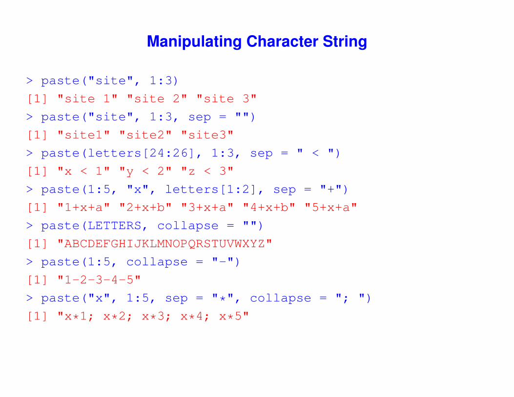
Manipulating Character String

> paste("site", 1:3)

[1] "site 1" "site 2" "site 3"

> paste("site", 1:3, sep = "")

[1] "site1" "site2" "site3"

> paste(letters[24:26], 1:3, sep = " < ")

[1] "x < 1" "y < 2" "z < 3"

> paste(1:5, "x", letters[1:2], sep = "+")

[1] "1+x+a" "2+x+b" "3+x+a" "4+x+b" "5+x+a"

> paste(LETTERS, collapse = "")

[1] "ABCDEFGHIJKLMNOPQRSTUVWXYZ"

> paste(1:5, collapse = "-")

[1] "1-2-3-4-5"

> paste("x", 1:5, sep = "*", collapse = "; ")

[1] "x*1; x*2; x*3; x*4; x*5"

Character substitution:

> sub("a", "?", c("aaa", "aba"))

[1] "?aa" "?ba"

> gsub("a", "?", c("aaa", "aba"))

[1] "???" "?b?"

Character substitution:

> sub("a", "?", c("aaa", "aba"))

[1] "?aa" "?ba"

> gsub("a", "?", c("aaa", "aba"))

[1] "???" "?b?"

Pattern searching:

> grep("A", LETTERS)

[1] 1

> grep("A", LETTERS, value = TRUE)

[1] "A"

> grep("a", LETTERS, value = TRUE)

character(0)

> grep("a", LETTERS, value = TRUE, ignore.case = TRUE)

[1] "A"

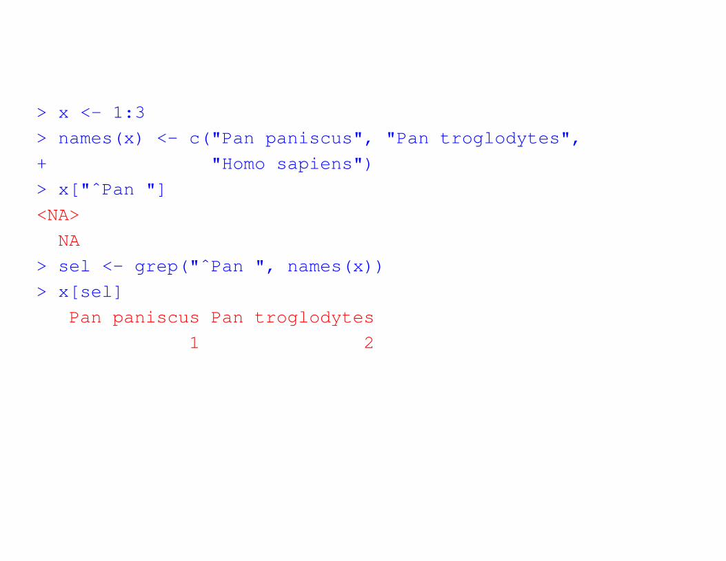
> x <- 1:3

> names(x) <- c("Pan paniscus", "Pan troglodytes",

+ "Homo sapiens")

> x["ˆPan "]

<NA>

NA

> sel <- grep("ˆPan ", names(x))

> x[sel]

Pan paniscus Pan troglodytes

1 2

Managing R scripts

A good editor allows to:

1. highlight the syntax,

2. show matching parentheses, brackets, and braces,

3. add and edit comments,

4. eventually send lines or blocks of commands directly into R.

Two main advantages in using scripts: repeating analyses, and adding comments.

To repeat analyses from a script:

1. copy/paste towards the console;2. send the commands to R (if possible);3. source("script Aedes morpho Dakar.R")

4. R CMD BATCH script Aedes morpho Dakar.R

With R CMD BATCH, the commands and the results are in the same file(‘script Aedes morpho Dakar.Rout’).

With source or R CMD BATCH, the comments must start with #.

Alternatively:

if (FALSE) {

..........

... block of commands not executed

........

}

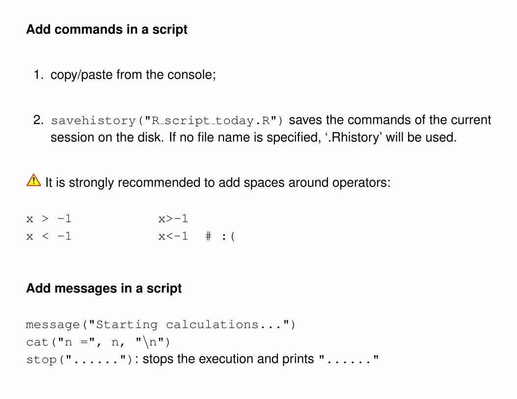
Add commands in a script

1. copy/paste from the console;

2. savehistory("R script today.R") saves the commands of the currentsession on the disk. If no file name is specified, ‘.Rhistory’ will be used.

It is strongly recommended to add spaces around operators:

x > -1 x>-1

x < -1 x<-1 # :(

Add commands in a script

1. copy/paste from the console;

2. savehistory("R script today.R") saves the commands of the currentsession on the disk. If no file name is specified, ‘.Rhistory’ will be used.

It is strongly recommended to add spaces around operators:

x > -1 x>-1

x < -1 x<-1 # :(

Add messages in a script

message("Starting calculations...")

cat("n =", n, "\n")stop("......"): stops the execution and prints "......"

R Programming

First program in R: assessing type I error rate of the t-test

p <- numeric(1000)

for (i in 1:1000) {

x <- rnorm(20)

y <- rnorm(20)

p[i] <- t.test(x, y)$p.value

}

hist(p)

sum(p < 0.05)

Q: How would you assess type II error rate?

II Data Structures in ape

Three things to know about ape. . .

� close to R’s logic⇒ integration with standard statistical methods

� concerns a continuum of users from “low” to “high” levels

� “evolving”: new methods, bug fixing, web site

. . . and many others http://ape.mpl.ird.fr/

ape’s friends

� ade4, apTreeshape, seqinrclose connections (data conversions, very few overlap in methods)

� RMesquitesoon to be released (based on R–Java communication)

� geiger, laser, phangorn, phylobase, . . .use ape and ade4 data structures

Trees

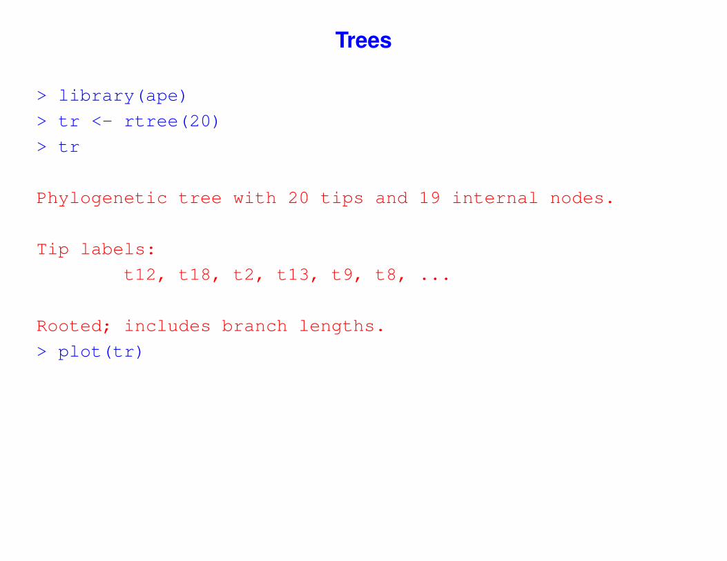
> library(ape)

> tr <- rtree(20)

> tr

Phylogenetic tree with 20 tips and 19 internal nodes.

Tip labels:

t12, t18, t2, t13, t9, t8, ...

Rooted; includes branch lengths.

> plot(tr)

Trees

> library(ape)

> tr <- rtree(20)

> tr

Phylogenetic tree with 20 tips and 19 internal nodes.

Tip labels:

t12, t18, t2, t13, t9, t8, ...

Rooted; includes branch lengths.

> plot(tr)

> is.rooted(tr)

[1] TRUE

> is.binary.tree(tr)

[1] TRUE

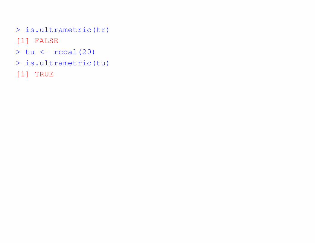
> is.ultrametric(tr)

[1] FALSE

> tu <- rcoal(20)

> is.ultrametric(tu)

[1] TRUE

> is.ultrametric(tr)

[1] FALSE

> tu <- rcoal(20)

> is.ultrametric(tu)

[1] TRUE

Lists of trees:

> TR <- rmtree(10, 20)

> TR

10 phylogenetic trees

> plot(TR)

DNA Sequences

DNA sequences in ape are stored in a special format (in the RAM; not on the disk).

> x <- c("a", "c", "g", "t")

> x <- as.DNAbin(x)

> x

1 DNA sequence in binary format.

> base.freq(x)

a c g t

0.25 0.25 0.25 0.25

What is not (yet) in ape:

� Amino acid sequences: see the package seqinr

� Allelic data (under development): see the package adegenet

� SNPs, microarray data, genotype–phenotype files, etc: see Bioconductor

� Networks (reticulated trees)

� Trees with singleton nodes (of degree 2)

The current tree data structure can be generalized for the last two.

III Input/Output with ape

read.tree reads tree(s) in Newick format

read.nexus same in Nexus format

read.dna reads DNA sequences in Phylip, FASTA, or Clustal formats (see theoption format)

read.GenBank reads DNA sequences from GenBank giving accession num-ber(s)

write.tree writes tree(s) in Newick format

write.nexus same in Nexus format

write.dna reads DNA sequences in Phylip or FASTA formats (see the optionformat)

IV Data Manipulation with ape

> TR[1:5]

5 phylogenetic trees

> TR[[1]]

Phylogenetic tree with 20 tips and 19 internal nodes.

Tip labels:

t2, t16, t17, t1, t19, t10, ...

Rooted; includes branch lengths.

Special functions for trees: root, unroot, drop.tip.

> data(woodmouse)

> summary(woodmouse)

15 DNA sequences in binary format stored in a matrix.

All sequences of same length: 965

Labels: No305 No304 No306 No0906S No0908S No0909S ...

Base composition:

a c g t

0.307 0.261 0.126 0.306

> dim(woodmouse)

[1] 15 965

> dim(woodmouse[, 1:300])

[1] 15 300

> dim(woodmouse[, c(TRUE, TRUE, FALSE)])

[1] 15 644

> dim(woodmouse[, !c(TRUE, TRUE, FALSE)])

[1] 15 321

Non-aligned sequences (i.e., from a FASTA file or from GenBank) are stored in alist.

Aligned sequences (i.e., from a Phylip or a Clustal file) are stored in a matrix.

as.matrix converts a list of sequences into a matrix if all sequences are of thesame length.

Exercices IV

1. Get the sequences from GenBank with accession numbersDQ082330-DQ082374. Examine this data set and see if you cancompute distances straight from it.

2. Align these sequences with Clustal (X or W). Read back thesequences into R.

3. Write eventually these commands into a script file, and repeat themfor AF006387–AF006459 with only the odd numbers.

4. Put both data sets into a single matrix, possibly dropping someobservations.

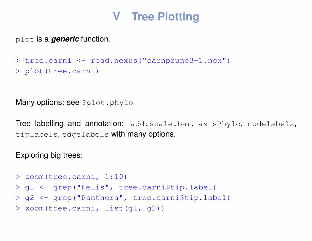
V Tree Plotting

plot is a generic function.

> tree.carni <- read.nexus("carnprune3-1.nex")

> plot(tree.carni)

Many options: see ?plot.phylo

Tree labelling and annotation: add.scale.bar, axisPhylo, nodelabels,tiplabels, edgelabels with many options.

Exploring big trees:

> zoom(tree.carni, 1:10)

> g1 <- grep("Felis", tree.carni$tip.label)

> g2 <- grep("Panthera", tree.carni$tip.label)

> zoom(tree.carni, list(g1, g2))

VI DNA Distances

> args(dist.dna)

function (x, model = "K80", variance = FALSE, gamma = FALSE,

pairwise.deletion = FALSE, base.freq = NULL,

as.matrix = FALSE)

See also the function dist to compute “geometric” distances. In both casesonly the lower triangle of the distance matrix is returned (except if the distanceis asymmetric), and is stored in a vector.

What is the influence of missing data and gaps?

> d <- dist.dna(woodmouse)

> dp <- dist.dna(woodmouse, pairwise.deletion = TRUE)

> summary(d)

Min. 1st Qu. Median Mean 3rd Qu. Max.

0.002201 0.009979 0.013350 0.013120 0.016740 0.022410

> summary(dp)

Min. 1st Qu. Median Mean 3rd Qu. Max.

0.002086 0.010520 0.013690 0.013350 0.016920 0.022280

> cor(d, dp)

[1] 0.9879206

> plot(d, dp)

> abline(a = 0, b = 1, lty = 3)

What is the influence of multiple substitutions?

> djc <- dist.dna(woodmouse, "JC69")

> dr <- dist.dna(woodmouse, "raw")

> plot(djc, dr)

> abline(a = 0, b = 1, lty = 3)

What is the influence of multiple substitutions?

> djc <- dist.dna(woodmouse, "JC69")

> dr <- dist.dna(woodmouse, "raw")

> plot(djc, dr)

> abline(a = 0, b = 1, lty = 3)

Exercices VI

1. Analyse the three data sets prepared previously with evolutionarydistances. Do any sort of analyses and explorations you may finduseful.

VII Tree Estimation

Distance Methods

Three methods available in ape: nj, bionj, fastme.bal (+ fastme.ols)

> tr.k80 <- nj(d)

> plot(tr.k80)

Does a different substitution model result in a different topology?

> tr.jc69 <- nj(djc)

> dist.topo(tr.k80, tr.jc69)

[1] 2

> plot(tc <- consensus(tr.k80, tr.jc69))

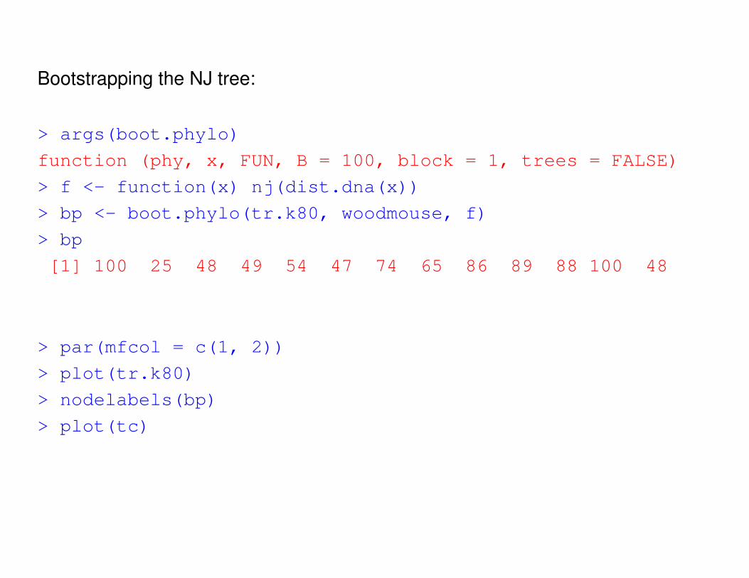
Bootstrapping the NJ tree:

> args(boot.phylo)

function (phy, x, FUN, B = 100, block = 1, trees = FALSE)

> f <- function(x) nj(dist.dna(x))

> bp <- boot.phylo(tr.k80, woodmouse, f)

> bp

[1] 100 25 48 49 54 47 74 65 86 89 88 100 48

> par(mfcol = c(1, 2))

> plot(tr.k80)

> nodelabels(bp)

> plot(tc)

What about the FastME method?

> tr.me.k80 <- fastme.bal(d)

> dist.topo(tr.k80, tr.me.k80)

[1] 6

> dist.topo(root(tr.k80, "No305"), tr.me.k80)

[1] 0

The topologies are the same.

Maximum Likelihood Methods

ML phylogeny estimation in R is in its early days. ape has an interface withPHYML:

> args(phymltest)

function (seqfile, format = "interleaved", itree = NULL,

exclude = NULL, execname, path2exec = NULL)

The trees estimated by PHYML can then be read into R with read.tree.

Bootstrapping is better done from PHYML; the tree then read with read.tree

has the bootstrap values in the element node.label.

Maximum Likelihood Methods

ML phylogeny estimation in R is in its early days. ape has an interface withPHYML:

> args(phymltest)

function (seqfile, format = "interleaved", itree = NULL,

exclude = NULL, execname, path2exec = NULL)

The trees estimated by PHYML can then be read into R with read.tree.

Bootstrapping is better done from PHYML; the tree then read with read.tree

has the bootstrap values in the element node.label.

The function mlphylo is in a beta-stage, and will provide soon various facilities(data partitioning, LRTs, . . . ).

Note the package phangorn which has an implementation similar to PHYML (NNI-rearrangements).

Other Methods

The package phangorn has parsimony methods for DNA sequences.

Bayesian methods may be implemented using existing tools in R (e.g., likelihoodcalculations, generating random trees).

FastME is currently based on NNI-rearrangements. A version based on SPR- andTBR-rearrangements has been written and is under testing.

Other Methods

The package phangorn has parsimony methods for DNA sequences.

Bayesian methods may be implemented using existing tools in R (e.g., likelihoodcalculations, generating random trees).

FastME is currently based on NNI-rearrangements. A version based on SPR- andTBR-rearrangements has been written and is under testing.

Exercices VII

1. Continue the analysis of the three data sets. Apply the sameguidelines than in the previous sections.

VIII Molecular Dating

Two main methods are available in ape:

1. The penalized likelihood (PL) method:

> args(chronopl)

function (phy, lambda, age.min = 1, age.max = NULL,

node = "root", S = 1, tol = 1e-08, CV = FALSE,

eval.max = 500, iter.max = 500, ...)

2. The mean path lengths method:

> args(chronoMPL)

function (phy, se = TRUE, test = TRUE)

(NPRS is obsolete and will be soon removed.)

Exercices VIII

1. Continue the analysis of the three data sets. Apply the sameguidelines than in the previous section.

IX Overview on Comparative Methods

> source("tree_macro.R")

You may have to resize the graphic window!

IX Overview on Comparative Methods

> source("tree_macro.R")

You may have to resize the graphic window!

Exercices IX

1. Do a phylogenetic comparative analysis of Carnivora body mass andlitter size with the files ‘carni data.txt’ and ‘carnprune3-1.nex’. You willuse the function pic as a starting point.

Many thanks to Celine, Selma & Christian for the

organisation of this workshop, and the University of

Graz for hosting it.