Any opinions and conclusions expressed herein are solely those of the author(s) and should not be construed as representing the opinions or

policy of any agency of the Federal government or the National Center for Family and Marriage Research.

2

FATHER INVOLVEMENT OVER TIME AND DIFFERENCES BY UNION STATUS:

A COMPARISON OF MOTHER AND FATHER REPORTS

Lauren Rinelli

Ph.D. Candidate

Department of Sociology

National Center for Family and Marriage Research

Bowling Green State University

lnrinel@bgsu.edu

*This is a draft. Please do not cite without permission from the author.

*The author would like to thank Susan L. Brown and Alfred DeMaris for their guidance and contributions to this

project, as well as Laura Sanchez, Kara Joyner, Wendy Manning and Deborah Wooldridge for their support. Also,

thanks to the National Center for Family and Marriage Research for supporting this research.

3

FATHER INVOLVEMENT OVER TIME AND DIFFERENCES BY UNION STATUS:

A COMPARISON OF MOTHER AND FATHER REPORTS

Collecting large-scale survey data is often expensive and time consuming. Many national surveys gather

information from one respondent who answers questions about members of the household or family.

Surveys about fertility or children typically target women only. While there are good reasons for this

strategy (e.g., women bear children and are usually their primary caregivers), researchers have begun to

realize that not having a male voice may bias results and yield an inaccurate picture of their side of the

story (Goldsheider & Kaufmann, 1996). In the past, the statistical methods available allowed only limited

comparisons of men’s and women’s reports of various constructs. However, newer, more sophisticated

statistical techniques now allow researchers to fully explore potential gender differences in reporting

(Coley & Morris, 2002). New data sets, such as Welfare, Children, and Families: A Three City Study and

the Fragile Families and Child Well-Being Study (hereafter referred to as Fragile Families), collect

information from both men and women, permitting comparisons of their reports.

The goal of the current study is to use men’s and women’s reports of father involvement to

determine the true couple mean level of involvement and the true discrepancy between their reports.

Until recently, many studies of father involvement rely on the mother’s report of the father’s behavior

(Bonney, Kelly, & Levant, 1999; Bronte-Tinkew, Ryan, Carrano, & Moore, 2007; Gaertner, Spinrad,

Eisenberg, & Greving, 2007; Knoester, Petts, & Eggebeen, 2007). Research shows that mothers typically

report lower levels of father involvement than fathers themselves report (Coley & Morris, 2002;

Mikelson, 2008). Furthermore, this pattern of findings depends in part on the parents’ living

arrangements. Mikelson shows that mothers and fathers are more likely to report different levels of

father’s physical involvement, but less likely to report different levels of emotional involvement when the

father and mother both live with the child than when the father is nonresident. Coley and Morris show

that there are certain characteristics associated with the mean level of father involvement and the

discrepancy between mother and father reports of father involvement, including level of conflict between

4

the parents. The more conflict parents report, the greater discrepancy in their reports of father

involvement. Although research by Coley and Morris and Mikelson is informative, there are a number of

shortcomings, discussed in detail below, the current study is able to overcome.

Father involvement is important for a number of reasons. First, society has moved beyond

concern with the simple presence or absence of fathers in their children’s lives. The expectation now is

for responsible fathering (Doherty, Kouneski, & Erickson, 1998), in which fathers are accessible,

engaged, and responsible (Lamb, Pleck, Charnov, & Levine, 1987). Accessibility means that the father is

physically and emotionally present and available to his children. Engagement has to do with the level of

interaction between father and child. This could mean playing games, reading books, telling stories, or

helping with homework. Fathers are responsible when they contribute to decisions about the child’s

welfare (e.g., which doctor the child should visit, what school they should attend), help with scheduling,

and take the child to appointments. Second, father involvement is associated with a number of positive

outcomes for children (see Lamb, 2004; Marsiglio, Amato, Day, & Lamb, 2000) and for men (Eggebeen

& Knoester, 2001; Knoester & Eggebeen, 2006). Third, the relationship between father involvement and

relationship quality seems to be reciprocal; the better the relationship between the parents, the more

involved the father is with his child (e.g., Anderson, Kohler, & Letiecq, 2002; DeLuccie, 2001; Fagan &

Barnett, 2003). Consequently, the more involved the father is with his child, the better the relationship

between the parents (e.g., Abidin, 1992; Bonney, Kelley, & Levant, 1999; Levy-Shiff, 1994; Romito,

Saurel-Cubizolles, & Lelong, 1999).

I first address the limitations of prior data collection and measurement strategies of father

involvement, followed by an overview of past literature that has attempted to unpack the similarities and

differences in reporting of father involvement by mothers and fathers. Next, I address my strategies for

improving upon prior work followed by a description of the data, measures, and analytic strategy that are

employed. Finally, I address the results and conclusions.

5

Data and Measurement Issues of Father Involvement

Surveys that include measures of father involvement typically use the household or the woman as

the enumeration unit. In these studies, one person in the household answers questions about other family

members who may or may not live in the household. Measurement error is plausible as the respondent

may truly not know the correct response, or their response may be conditioned by some other factor, such

as relationship status with person of interest. Without research to closely examine these possibilities, we

remain uncertain under what conditions and when it is appropriate to use mother’s reports about the

father’s behavior.

Surveys such as the National Survey of Families and Households attempt to obtain information

from the main respondent’s spouse or partner, perhaps even after the couple is no longer romantically

involved at a follow-up wave. While much can be gained from these techniques, they are costly and

involve some risk. Men are subject to a higher nonresponse rate than women, particularly if they are not

living in the same household as the main respondent (Carlson, McLanahan, & Brooks-Gunn, 2008;

Mikelson, 2008).

Researchers’ conceptualization of father involvement has evolved over the years. The role of the

father has long been considered one of financial support; however, in recent decades, the notion of

responsible fathering has emerged. Lamb, Pleck, Charnov, and Levine (1985, 1987) posit three

dimensions of father involvement, including accessibility, engagement, and responsibility. Mikelson

(2008) measures physical involvement and emotional involvement. Studies within the psychological

literature have emphasized the use of time-diaries or parental observations as important methods of data

collection beyond surveys. Current surveys do not always reflect these new conceptualizations of father

involvement, resulting in inconsistent measures between surveys and a lack of various dimensions of

father involvement.

6

Not only have there been problems with data collection techniques and measurement strategies,

but statistical analyses of reporting differences, until recently, have been limited to paired t-tests, which

can only determine whether there is a mean difference in reporting on a particular item. Statistical

techniques have evolved to include hierarchical linear modeling, which can determine the true mean score

on a given item by both reporters and a true discrepancy score, which indicates the difference between the

reporters’ scores while taking into account the correlation of the dyad (Coley & Morris, 2002). This

technique allows the researcher to control for other characteristics of the individuals and the dyad to

determine what factors influence the level of discrepancy between reporters (Raudenbush, Brennan, &

Barnett, 1995).

Prior literature on Reporting of Father Involvement

Two studies have directly compared mother and father reports of father involvement. First, Coley

and Morris (2002) use data from Welfare, Children, and Families. Second, a Three Cities Study compares

mother and father reports of father involvement and then employ paired hierarchical linear modeling to

find the true dyadic mean and the true discrepancy score between parents’ reports. This is the first and

only paper to utilize this technique to compare mother and father reports of father involvement. Coley

and Morris construct a six-item scale to operationalize father involvement. Three questions, with a four-

point scale of responses ranging from 1 (none) to 4 (a lot), are (1) “How much responsibility does [father]

take for raising child?”; (2) “How much does [father’s] involvement make things easier for [child’s

mother] or make [her] a better parent?”; and (3) “How much does [father’s] help with financial and

material support of child help [mother]?” Three other questions were recoded to match the 4-point scale

of the first three questions and include original responses of number of hours, a 5-point scale and a 6-

point scale, respectively, ask: (4) “How many hours per week does [father] take care of child?”; (5) “How

often does [father] see or visit with child?”; and (6) “How often does child see or visit with [father’s]

family?” Although these items load on a single factor, only questions 1, 4, and 5 are direct measures of

father involvement. The other questions appear to measure how much the mother benefits from the

7

father’s involvement (questions 2 and 3) and the level of contact with extended family (which may or

may not involve the father himself - question 6). Although this measurement strategy includes more

items than had been examined previously on the subject of father involvement, these items may not fully

capture the concept of father involvement as specified by Lamb and colleagues (1985) as accessibility,

engagement, and responsibility.

Nonetheless, Coley and Morris find that across the six items, 61 percent of mothers and fathers are

in exact agreement. Furthermore, 75 percent of coresident pairs agree, whereas only 48 percent of

noncoresiding pairs agree on the level of father involvement, on average, across the six items. The HLM

analyses reveal that the average item score is 3.15, which is a moderately high level of father involvement

reported by parents. The true discrepancy score is -1.37, which indicates that mothers, on average, report

a level of involvement 1.37 units lower than fathers report. When fathers are employed full time and

when fathers live with their child, the true couple-mean level of father involvement is higher. The more

time elapsed between the mother’s and father’s interview and higher levels of conflict between the

parents, the lower the level of father involvement. Additionally, the interaction term, father residency by

employment status, indicates that employed resident fathers and unemployed resident fathers do not

significantly differ in their level of involvement, but employed nonresident fathers are more involved than

unemployed nonresident fathers. This result is consistent with Townsend’s (2002) findings that fathers

who felt they could not provide financially for their children withdrew and were not as involved (Lamb,

1997; Liebow, 1967). It is also possible that mothers do not allow fathers to be as involved when they

cannot provide financially for their children; however, these explanations were not tested.

The multivariate results reveal a number of characteristics associated with greater discrepancy

between mother and father reports of father involvement. Father’s age, mother’s education, maternal

employment, conflict, and time between interviews are associated with a greater discrepancy score

between mothers and fathers. In other words, these characteristics are associated with mothers reporting

lower levels of father involvement than fathers report. Coley and Morris (2002) offer possible

8

explanations for the association between these variables and discrepancy; older fathers may have more

children (and possibly by other mothers), so their time is not as concentrated on the focal child. Maternal

employment and education may lead to higher expectations of father involvement, which may “color”

mother’s images of father involvement, resulting in divergent reports. Alternatively, because of their

greater need for involvement by fathers, working mother’s perceptions of father involvement may be

lower than desired. Couples who experience a higher level of conflict may have greater discrepancy

scores due to (1) mothers intentionally or unintentionally reporting lower levels of father involvement, (2)

fathers inflating their reports of involvement to look better, and/or (3) in part, conflict may be due to

differing ideas about the appropriate level of involvement, which may lead to differences in reporting.

Finally, Coley and Morris note that a larger gap in time between interviews may be indicative of

disorganization or contention within the family, thus resulting in differences between mothers’ and

fathers’ reports of involvement.

Mikelson (2008) conducts a similar study using cross-sectional data from Wave III of the Fragile

Families. Many studies that use Fragile Families data to examine the association between father

involvement and child and families outcomes only use reports of father involvement obtained from the

mother. Given that data from the father are available, it is possible to empirically evaluate whether this is

a good strategy, which is a goal of Mikelson’s research. It must be acknowledged that missing data for

fathers in the Fragile Families study is sizeable and nonrandom. In other words, fathers’ participation in

the survey is related to their relationship status with the mother, with married and cohabiting fathers most

likely to be included and fathers who are no longer romantically involved with the mother least likely to

be surveyed. In fact, Fragile Families is most representative of cohabiting fathers and least representative

of visiting and nonromantic fathers with married fathers in between (Carlson, McLanahan, & Brooks-

Gunn, 2008). A more detailed discussion of missing data for fathers in the Fragile Families data is

presented below.

9

Mikelson does not use the same analytic strategy as Coley and Morris (2002). Instead, she

simply creates a difference score by subtracting father’s reported involvement from mother’s reported

level of father involvement and used OLS regression to determine what factors were associated with the

difference. Fragile Families includes a much more extensive set of father involvement indicators than

other datasets, including the Three Cities Study, therefore, Mikelson is able to focus on both physical

involvement (e.g., singing songs, playing with toys, putting child to bed) and emotional involvement (e.g.,

shows affection to child). There are 11 indicators of physical involvement and 2 indicators of emotional

involvement. Furthermore, mothers and fathers are asked on how many days in a typical week the father

does a particular activity. This is a more precise measure than the 4-point scale used by Coley and Morris

(2002) and is perhaps the most comprehensive operationalization of father involvement available in any

recent dataset.

Mikelson’s conclusions regarding physical father involvement differ depending on how

agreement/disagreement is defined. When mother reports are subtracted from father reports, fathers

indicate more days of involvement than mothers on all 11 items, and those differences are statistically

significant. However, when differences are constructed between resident father and mother reports and

nonresident father and mother reports, resident fathers and mothers exhibit greater levels of disagreement.

For instance, resident father-mother disagreement on assisting the child with eating and putting the child

to bed is higher than nonresident father-mother disagreement. This finding is contradicted, however, if

exact agreement is considered. The level of exact agreement between resident father-mother pairs is

higher than between nonresident father-mother pairs.

These findings reveal that whose report is considered or, if both parents’ reports are utilized, how

the reports are combined yield different conclusions about levels of father involvement; however, reports

of emotional involvement are not as inconsistent as physical involvement (Mikelson, 2008). The

descriptive results show that although both mothers and fathers report high levels of emotional

involvement, resident fathers-mothers have higher levels of agreement, regardless of the definition of

10

agreement, than do nonresident father-mother pairs. It is possible that mothers and fathers agree that

fathers love their child but disagree about day-to-day care and activities fathers engage in with their

children.

Mikelson’s (2008) OLS regression results coincide with prior findings, which show that father-

mother discrepancy is lower (i.e., there is more agreement) when mothers report having a good

relationship with the father and when the parents are married. On the other hand, father-mother

discrepancy is higher (i.e., there is less agreement) when (1) the father lives with the child (and the

mother), (2) the mother has received financial help from anyone except the father since the child was

born, (3) the father reports having a good relationship with the mother, (4) and there is a greater difference

in the child’s age at the time of the father’s interview (i.e., there is a larger amount of time between the

mother’s and father’s interview). These results, as well as the results from the Coley and Morris research,

indicate the importance of father residency, relationship status, and relationship quality in the level of

agreement between mother’s and father’s reports of father involvement.

While both of these studies greatly contribute to our understanding of reporting on father

involvement, there are a few limitations that I address with the current study. First, Coley and Morris

focus on children between the ages of two and four. Children are aged three at the time of the survey

Mikelson utilizes. The current study extends prior work by analyzing reports of father involvement when

children are one, three, and five years old. This strategy allows for an examination of father involvement

at different stages of children’s development as well as how father involvement changes over time.

Additionally, during the five years of observation, parents’ relationship status and father residency

may change. Including measures of union stability and transitions allows for an analysis of the level of

father involvement in different family structures and the extent to which union type/transition is

associated with the dyad’s report of father involvement (i.e., discrepancy between reporters). The

association between father residency and involvement was not consistent between the two prior studies,

11

perhaps due to their cross-sectional nature. The current investigation may shed light on the discrepant

findings by accounting for change over time.

Finally, Coley and Morris use a 4-point scale, which indicates (4) a lot to (1) no father

involvement on a given item. Mikelson’s measurement, on the other hand, considers the number of days

of involvement on a given item. I argue, as Mikelson does, that the number of days a father is involved in

a given activity is a more precise measure than whether the father is involved a lot or a little. It should be

acknowledged, however, that time-diary data arguably would be the best method to precisely measure the

time fathers spend with their children. The number of days per week does not give any indication of how

much time fathers are with their children during the day (e.g., the whole day versus just a few minutes at

bedtime); therefore, this measure is not necessarily ideal. Nonetheless, days per week is the only

available measurement of father involvement in Fragile Families, therefore, the number of days of

involvement which replicates and extends Mikelson’s work with more sophisticated statistical techniques,

namely dyadic hierarchical linear modeling is used

THE CURRENT STUDY

The current investigation focuses on the level of father involvement among families with a new

child, the similarities and differences in reporting of father involvement between mothers and fathers in

the Fragile Families data and the factors associated with those similarities and differences, particularly

union status and union transitions. The issue pertaining to similarities or differences in reporting of father

involvement is that mothers and fathers are reporting on the same phenomenon, namely the father’s

behavior. The father is asked about his own behavior while the mother is asked about her perception of

the father’s behavior. In other words, since they are both being asked to report on the same behavior,

their responses presumably should be the same. Differences in reporting may be because the mother is

not sure of how involved the father is, particularly when he is non-resident. Differences may also stem

from her perceptions of him as a person. For example, if he does not invest a lot of time in his work, she

may think he is equally lazy with his children. Finally, differences may stem from the father

12

overestimating his level of involvement because of social desirability factors. It is also possible,

although most mothers report lower levels of involvement than fathers themselves report, some mothers

may overestimate fathers’ level of involvement due to social desirability factors as well.

There are a number of questions to be addressed by this research. First, what is the level of father

involvement as reported by mothers and fathers, and how much discrepancy exists between their reports?

Based on the work of Coley and Morris (2002), I expect two hypotheses: (1) a moderate level of father

involvement (i.e., about 3-4 days per week) and (2) mothers to report slightly less involvement by fathers

than fathers report.

Second, how does the level of father involvement and the discrepancy between reporters change

over time? In the first few months of a child’s life, research shows a decline in most types of father

involvement (Belsky & Volling, 1987). Yueng, Sandberg, Davis-Kean, and Hofferth (2001), using time-

diary data, show that the absolute level of father involvement decreases as children age. However, Lamb

(2000) reports that fathers spend more time with older rather than younger children. Bruce & Fox (1999)

conclude that the relationship between father involvement and child age is curvilinear; fathers spend the

most time with children when they are in their preschool years. It is possible that inconsistencies in these

results are due to differences in research designs and measurement strategies, operationalization of father

involvement, and observation periods at differing points in children’s lives. Consequently, most of the

research over the study’s observation period shows a decline in the trajectory of the level of father

involvement, therefore, I expect this pattern to emerge as a third hypothesis. This study is the first to look

at discrepancy in reports over time. Theory does not provide a guiding hypothesis, therefore, I am not

specifying a priori whether or how it will change (hypothesis 4 – not specified).

Third, is there a higher level of father involvement and a higher level of agreement among couples

who are married or cohabiting (i.e., resident) than among couples who are visiting or not romantically

involved (i.e., nonresident)? Mikelson (2008) found there to be more agreement between mother’s and

father’s reports of physical involvement when the father is nonresident. While that finding seems

13

counterintuitive, the measurement of involvement was the average number of days per week. If, for

example, the nonresident father has his child two days per week, mothers and fathers would both report

his frequency of involvement as two days per week, which results in higher levels of agreement than

among resident parents with no set schedule. Therefore, I hypothesize that when fathers are visiting or

not romantically involved with the mother, there will be lower levels of involvement than among married

and cohabiting fathers (hypothesis 5) but more agreement between mother and father reports (hypothesis

6). It is also of interest to compare father involvement between married and cohabiting couples. Given

their less traditional gender role attitudes (DeMaris & MacDonald, 2003), cohabiting couples may

experience a higher level of father involvement than marrieds (hypothesis 7). Alternatively, the fact that

the couple is unmarried ostensibly demonstrates less commitment to the mother and family, suggesting

lower levels of father involvement among cohabitors than marrieds (hypothesis 8). I test these competing

hypotheses.

Finally, are characteristics of the father, mother, child, and dyad associated with the level of father

involvement and/or the level of discrepancy between reporters? These variables will be included as

controls. These types of variables have been used in prior studies of father involvement and discrepancy

in reporting (Coley & Morris, 2002; Mikelson, 2008), as well as in studies on union stability and

transitions (e.g., Brown, 2000; Carlson, McLanahan, & England, 2004; Harknett & McLanahan, 2004).

DATA

This research uses data from the Fragile Families, which are representative of births in 2000 in cities with

populations over 200,000. The baseline survey was collected between 1998 and 2000. Mothers were

interviewed in the hospital within 48 hours after giving birth. The father was interviewed in the hospital

or as soon after the birth as possible. Mothers and fathers were interviewed at the child’s first, third, and

fifth birthdays. For additional sampling and data information for the first three waves of data, see

Reichman and colleagues (2001).

14

Fragile Families is more representative of fathers than other datasets collected in recent years;

obtaining information from fathers, particularly unwed fathers, was a central goal and guided much of the

research protocol. However, missing data for fathers is an important issue when using the Fragile

Families data, particularly for the later waves. Based on the number of completed mother interviews at

Time 0; 79 percent of fathers were interviewed at Time 0; 70 percent at Time 1; 67 percent at Time 3; and

65 percent at Time 5. Fathers’ participation in the Fragile Families study is related to their involvement

with the mother (Carlson et. al., 2004); married (89%), cohabiting (90%), followed by visiting fathers

(73%). Fathers who are friends with the mother (53%) or who are no longer romantically involved with

the mother at the time of birth (28%) are least likely to be in the sample (figures at Time 0). See Table 1

for father response rates by relationship status at each wave. It is clear that missing data (and attrition) for

fathers are not random. Missing data and attrition most likely occur when fathers are not living with

mothers, are not romantically involved, or have no relationship. As a result of this non-random non-

response, fathers with the lowest level of involvement with their children are least likely to be included in

the Fragile Families data, so results presented are most likely to be representative of fathers with higher

levels of father involvement.

Fragile Families data are based on 4,898 births. I only include parents for which the father is

known and each member of the dyad is interviewed at least one time. This limitation yields 4,224

mother-father pairs.

MEASURES

The purpose of this analysis is to compare mother and father reports of father involvement.

Therefore, each measure discussed below, unless otherwise specified, is created for mothers and fathers

separately. Mean substitution is used to handle missing data on continuous independent variables and

modal substitution is used for categorical and dichotomous variables. Missing data on the dependent

variable is left missing.

15

Dependent Variable: Father Involvement

Mothers and fathers are asked to report the number of days per week the father performs a number

of activities at Times 1, 3, and 5. Of central importance to this research question is how father

involvement changes over time, thus, analogous measures are needed across waves. However, only four

items are the same at each interview: sings songs or nursery rhymes to child, reads stories, tells stories,

plays inside with toys such as blocks or Legos® (original coding is maintained). Unfortunately, there are

some limitations that stem from using only these four measures. First, I am not tapping into Lamb and

colleagues’ (1985) three dimensions of father involvement, including accessibility, engagement, and

responsibility. These four items would be considered measures of engagement; however, this does not

represent the full range of possible engagement items. Furthermore, these items do not measure

emotional involvement, nor are they developmentally specific. To get a good understanding of change in

measures over time, the same items are needed. Fragile Families changes and adds new measures at each

wave, which are developmentally specific, however, they cannot be used in the current analysis as the

items change across waves.

To use dyadic growth curve analysis, it is necessary to create parallel scales of father involvement

measures for mothers and fathers at each wave (1, 3, and 5). Parallel scales are two separate scales (Scale

A and Scale B) created by splitting the items that measure a given concept so that the scales have equal

variance and equal reliability (Raudenbush, Brennan, & Barnett, 1995; Sayer & Klute, 2005). To do this,

four measures are ordered from lowest to highest standard deviation. Then, two by two, one measure is

randomly selected for Scale A and the other for Scale B until all four measures have been used to create

two separate parallel scales for mothers (i.e., two iterations of pairing items and assigning them to either

Scale A or Scale B). For example, for items ordered 1 through 4, I randomly assign Item 1 to either Scale

A or Scale B; item 2 is then put in the other Scale. This procedure is followed again for Items 3 and 4, so

all four items are assigned to either Scale A or Scale B (two items per scale). This process is repeated to

16

create two separate parallel scales for fathers, and again for mothers and fathers at each wave (1, 3, and

5). Thus, each dyad contributes a total of 12 scales, ranging from 0 to 7 days per week. The goal of this

strategy is to account for measurement error and increase the likelihood that these measures reliably tap

the underlying concept of father involvement. When specifying the models, there is only one father

involvement scale variable, which will be created from these separate parallel scales for each reporter at

each wave. For a more detailed explanation of parallel scales, see Raudenbush, Brennan, & Barnett

(1995) or Sayer & Klute (2005).

Independent Variables

To measure the level of discrepancy between mother’s and father’s reports of father involvement,

gender gap is coded as 0.5 for mothers and -0.5 for fathers. This coding strategy is appropriate to yield an

intercept which represents the average true couple mean father involvement (i.e., gender gap = 0).

Time is coded in years since the initial interview (birth of child); 1, 3, and 5 years.

Union Status and Transitions: Central to the hypotheses about agreement or disagreement in

mother’s and father’s reports of father involvement is the relationship status of the parents. The coding

used, between-subjects union status/transition dummies, tells us the relationship trajectory over the

observation period. This approach is advantageous as it allows for an examination of the level of father

involvement over time for each group, as well as an investigation of the discrepancy between mother and

father reports by relationship status. This approach may help researchers determine when it is appropriate

to use only mother reports of father involvement and when it may be limiting. This approach has a

limitation: it is not possible to examine the level of father involvement both before and after a change in

union status between waves (i.e., this strategy does not reveal whether a transition occurred between

Times 0 and 1, Times 1 and 2, Times 2 and 3, or Times 3 and 4). There would be a total of 36 possible

transitions if these dummies were coded between each wave. For parsimony, I chose to use the single set

of union status/transition dummies over the entire observation period.

17

Using a series of questions about the parents’ current relationship status and living arrangements

from mothers’ reports (unless the mother’s report is missing, then the father’s report is used if available),

Fragile Families constructs the parents’ union status at the beginning of each wave. The constructed

variable is recoded into a categorical variable: (1) married, (2) cohabiting, (3) visiting, and (4)

nonromantic at each wave. A set of between-subjects dummies is then created to indicate stability or

transition over the five-year observation period. The categories are as follows: continuously married,

continuously cohabiting, continuously visiting, or continuously nonromantic (combined into one

category), cohabiting to married, cohabiting to not cohabiting (visiting or nonromantic), married to not

married, visiting/nonromantic to cohabiting, visiting/nonromantic to married, between visiting and

nonromantic (either direction), two or three transitions1.2

Father and Mother Characteristics: Mother’s and father’s education are both taken from self-

reports. Each parent reports their highest level of education at baseline. Constructed dummy variables

are created indicating whether the father (mother) has less than a high school degree, a high school

diploma or equivalent (reference), some college or technical training, or a college degree or above.

Missing cases are recoded to the modal category (mothers-less than high school, fathers-high school

diploma or equivalent). The constructed variable of father’s age measured in years at baseline is

included. As mother’s age and father’s age are highly correlated (.95), only father’s age is included.

Child Characteristics: Child gender is associated with father involvement such that fathers are

more involved with sons than daughters, on average (Barnett & Baruch; 19897; Lamb, Pleck, & Levine,

1987). Additionally, sons are related to higher levels of marital stability (Katzev, Warner, & Acock, 1994;

Morgan, Lye, & Condran, 1988; Mott, 1994; Spanier & Glick, 1981) and increased likelihoods of

1 When categorizing the possible two or three transitions, cell size become too small to analyze all possible transitions, thus two

transitions and three transitions dummies are created. There is no statistical difference in any models in experiencing two

versus three transitions, thus they are combined for the sake of parsimony.

2 There are 856 cases for which union status at one or more waves is missing. As union status/transition is the focal

independent variable, I choose not to replace missing data. These cases are dropped in the analysis at waves that are missing.

18

cohabiting couples to transition to marriage (Lundberg & Rose, 2003), although some of these

associations may have become weaker over time (Lundberg, McLanahan, & Rose, 2007; Pollard

&Morgan, 2002). Therefore, child gender may be associated with the level of father involvement.

Gender of child is taken from the mother’s baseline survey: boy (1), girl (0). Fragile Families constructs a

variable indicating whether the focal child was considered low birth weight. Original coding of this

variable is maintained: (1) low-birth weight, (0) normal weight. At each wave, fathers are asked about

their child’s overall health, ranging from (1) very poor to (5) excellent. Due to the skewed distribution, a

time-varying dummy is created indicating father reports child’s health as excellent (1) or less than

excellent (0). Fathers’ reports are used instead of mothers’ reports because what is real to the individual is

real in its consequences, meaning that fathers’ own perspectives of their child’s health may be more

important to his level of involvement than the mother’s report.

Dyad Characteristics: Based on questions of racial and ethnic background, Fragile Families

constructs a race variable from which dummies are created to indicate the parents are both non-Hispanic

White (reference), non-Hispanic Black, Hispanic, of another racial/ethnic background, or the parents are

from different racial/ethnic backgrounds. Missing cases are recoded to the modal category (non-Hispanic

Black).

Multipartner fertility has become an increasingly prevalent phenomenon among unmarried couples

and couples who have married following a prior marital or cohabiting union. Particularly when studying

father involvement, taking into consideration the number and composition of children mothers and fathers

have is important, as fathers are likely to spend more time with focal children who are their only children.

Fathers who have older children or children by other mothers have to spread their time between children,

which oftentimes results in less involvement with the focal child (Carlson & Furstenberg, 2006). Mothers

and fathers are asked at each wave how many children they have together and how many children they

have by other partners. Using these questions, it is determined whether the dyad has only the focal child

(reference), only biological children together, the mother has children who are not biologically related to

19

the father, the father has children who are not biologically related to the mother, or both parents have

other biological children. These variables will be time-varying.3 Note that other children, if present, are

not necessarily living in the same household as the focal child and/or the father.

At each interview, mothers and fathers are asked to report the number of hours worked per week at

their current or most recent job. Dummy variables are created for fathers (mothers) at each wave

indicating father (mother) does not work or works part-time (0) or works full-time (1).4 Next, a set of

time-varying labor force participation dummies is created to indicate both mother and father work full-

time (reference), father only works full-time, mother only works full-time, neither mother nor father works

full-time.

There is a constructed measure at each wave, which indicates the time difference between the

mother and father interviews. At each wave, it has been recoded in days, with negative numbers

indicating that the father was interviewed first, positive numbers indicating that the mother was

interviewed first, and 0 indicting they were interviewed on the same day (e.g., -15 = father was

interviewed 15 days before the mother, 20 = mother was interviewed 20 days before the father). This is

necessary to include because differences in reporting may be simply because mothers and fathers are

reporting on different time periods in the child’s life, even though questions are not asked about a specific

time period. Furthermore, efforts were made to interview parents as close to each other as possible

(Reichman et al., 2001). A long time-period between interviews may indicate that the mother did not

know how to contact the father or other issues that may signify problems between parents.

ANALYTIC STRATEGY

I employ univariate hierarchical linear modeling (HLM), also known as linear mixed effects modeling

(LMEM). HLM is the appropriate modeling strategy because individual mother and father variables are

3 Information from Time 5 is not as complete as it is for the first three waves. Many assumptions would have to be made to include data from

Time 5, therefore, I copy information from Time 3 at Time 5. Results in reference to Time 5 should be interpreted with caution. 4 Due to small cell sizes, I decided to collapse not working and working part-time into one category.

20

nested within dyads. HLM is a superior method to traditional statistical techniques such as multiple

regression or RMANOVA because it takes account of the dependency between reporters and accounts for

measurement error. For a more detailed explanation of the advantages of multilevel modeling, see Lyons

and Sayer (2005), Raudenbush, Brennan, and Barnett (1995), and Sayer and Klute (2005). I will use

measures of father involvement from Times 1, 3, and 5 as the measures are consistent between waves

(note: Time 0 measures father’s involvement with the mother during pregnancy and are not the same as

measures of his involvement with the child in the follow-up waves, making this strategy the most

appropriate).

Father Involvement Hypotheses and Analyses

Mothers and fathers report a moderate level of father involvement, although mothers report a

lower level of father involvement than fathers report. To test these hypotheses, I create parallel father

involvement scales at each wave based on mothers’ and fathers’ reports (see description in Measures

section). The intercept only model is the unconditional means model which shows the true couple mean

level of father involvement. Then the gender gap variable is entered in the unconditional gender gap

model. The coefficient for the gender gap variable is the true discrepancy score between mothers’ and

fathers’ reports of father involvement.

The level of father involvement will decrease over time. To test this hypothesis, time is added in

the unconditional gender gap and growth model. The coefficient for time shows the trajectory of change

in the level of father involvement over the observation period. How does the level of discrepancy change

over time? Including an interaction term between gender gap and time will describe how the level of

discrepancy changes over time.

The level of father involvement is higher among married and cohabiting couples than among

visiting or nonromantic couples. Father involvement may be higher among cohabiting couples than

among married couples or it may be higher among married couples than among cohabiting couples. The

union status stability/transition dummy variables are entered in the model. To determine differences

21

between the contrasts of interest, the reference category is changed between models. The level of

discrepancy between parents is higher when they are resident (married or cohabiting) than when they are

nonresident (visiting or nonromantic). When the dummies are interacted with gender gap, it can be

determined how relationship status influences discrepancy between reporters.

What factors contribute to the level of father involvement and the discrepancy between reporters?

Characteristics of the father, mother, child, and dyad are entered in the final model. The intercept is the

average level of father involvement controlling for those factors. The coefficient for the gender gap is the

average level of discrepancy between reporters, all else being equal. Interactions between these

characteristics and the gender gap are tested but only significant ones are discussed in the results section.

RESULTS

Descriptive Statistics

Descriptive statistics for the current investigations are shown in Table 2.2. For time-varying variables, the

mean is the average over the observation period.

Father Involvement

The average level of father involvement, both within and between sets of parents, is 3.38 days per

week. Table 2.3 shows the average level of father involvement at each wave by reporter. At each time

point, fathers report a higher level of involvement than mothers report. Fathers report a linear decline in

involvement over time, whereas mothers report slightly higher levels of involvement at Time 3 than at

Time 1 and then report a decline at Time 5. The pattern is shown graphically in Figure 2.1. It does not

appear that there is an interaction between the gender gap in reporting and time.

Union Status/Transitions

Twenty two percent of the sample remains married for the five years under observation, seven percent

continuously cohabit, and seven percent remain either continuously visiting or continuously nonromantic

over time. Therefore, only 36 percent of this sample remains in a stable family form over the first five

years of a child’s life. The remaining 64 percent experience at least one transition; 16 percent experience

22

two transitions and 6 percent experience three transitions (not shown). Of the 42 percent who

experience one transition, there are six possible transition captured here. Table 2.4 shows the transitions

that occur by union status at birth. Of those parents who are married at birth, 81 percent remain married

over the observation period, 16 percent divorce, and three percent experience two or three transitions with

the other biological parent. Not surprisingly, parents who are married at birth have the most stable

unions. Among those cohabiting at the child’s birth, 19 percent remain in long-term cohabiting unions,

22 percent transition to marriage, 34 percent separate, and 25 percent experience two or three transitions.

Forty one (19 + 22) percent of parents who are cohabiting at the child’s birth actually remain in stable

unions over the five years of observation. Parents who are in visiting relationships or who are not

romantically involved at the child’s birth are the most unstable. Nineteen percent remain visiting or

nonromantic over five years, four percent transition to marriage, and eight percent move in together but

do not marry. Thirty-seven percent transition between visiting and being nonromantic (in either direction)

one time, and Thirty-two percent make two or three transitions. Clearly, these parents experience the

most transitions, which may or may not include movements of the father in and out of the household, and

the most time at separate residences.

Figure 2.2 shows average father involvement by union or transition status over time and Table 2.5

shows the analysis of variance (Tukey) results at each wave with the significant mean differences between

groups highlighted. At Time 1, parents who transition from cohabitation to marriage exhibit the highest

levels of father involvement, followed closely by those who continuously cohabit, are continuously

married, or those who are visiting/nonromantic at birth but transition into marriage (differences not

significant). By Time 3, those who transition from visiting/nonromantic to either cohabitation or

marriage have levels of involvement, which are statistically the same as the three continuously resident

groups. By Time 5, however, the fathers who have transitioned from visiting/nonromantic to married

have the highest levels of involvement, although it is not statistically different from the continuously

married or cohabiting, cohabiting to married, or visiting/nonromantic to cohabiting groups. The three

23

groups that experience the sharpest decline in involvement are parents who experience a divorce,

parents who experience two or three transitions, and parents who were cohabiting and then break up. By

Time 5, it appears that cohabiting parents who separate report slightly higher levels of involvement than

married parents who divorce; however, this difference is not significant. Clearly, visiting parents and

parents who are nonromantic have the lowest levels of involvement. Whether these states are continuous

or there is a transition between the two, fathers who are continuously nonresident exhibit the lowest levels

of involvement at all time points. By Time 5, fathers who are nonresident spend, on average, about two

days per week with their children.

Father Characteristics

Among fathers, 31 percent have less than a high school degree, 37 percent have received a high

school diploma, 21 percent have attended college but did not finish, and 11 percent have earned a college

degree. On average, fathers are about 28 years old at their child’s birth.

Mother Characteristics

About 33 percent of mothers did not receive a high school diploma, about 30 percent earned their

high school degree, 25 percent have some college education, and 12 percent have received a college

degree. On average, mothers are 25 years old at their child’s birth. Mother’s and father’s age is highly

correlated (.95), therefore, only father age is included in the analysis.

Child Characteristics

Fifty two percent of focal children in this sample are boys. About nine percent of focal children

were considered low birth weight. Across waves, 64 percent of fathers (or mothers, if missing for fathers)

rate their child’s health as excellent.

Dyadic Characteristics

Seventeen percent of couples are White, 44 percent are Black, 22 percent are Hispanic, two

percent are of other racial/ethnic backgrounds, and 15 percent of couples are interracial. Across the first

three waves, time-varying dummies are included to indicate whether multipartner fertility exists among

24

parents in this sample. For 19 percent of couples, the focal child is their only child, across all time

points. About 28 percent of couples have more than one biological child together. Sixteen percent of

couples involve at least one child who biologically belongs to the mother but not the father, 17 percent

have a child who is biologically the father’s but not the mother’s, and 19 percent of parents both have

children by other partners. Almost 57 percent of parents both work full-time. In 17 percent of dyads,

only the father works full-time, in 7 percent of dyads, only the mother works full-time, and in 5 percent of

dyads, neither parent works full-time. Across waves, the average time difference between mother and

father interviews is about 43 days (mother interviewed first).

Dyadic Univariate Hierarchical Linear Models

The unconditional means model, Table 2.6A Model 1, shows first that 34 percent of the variance

in father involvement is between sets of parents and 66 percent of the variance is within sets of parents.

The intercept, or the true couple mean level of father involvement, is 3.25, which indicates, on average,

couples report fathers are involved with their children about half of the week (recall the father

involvement scale ranges from 0 to 7 days). There is significant variability in couple average father

involvement across couples.

The variable for gender gap is added in the unconditional gender gap model. Nineteen percent of

the variability in reports of father involvement within couples is accounted for by gender. The AIC and

BIC have dropped, which indicates that the model is an improvement over the unconditional means

model. Average mean father involvement is 3.28 and mothers, on average, report father involvement to

be 0.56 days less than fathers report. The results from Models 1 and 2 lend support for Hypotheses 1 and

2; parents report a moderate level of father involvement, with mothers reporting lower levels of

involvement than fathers report.

To test Hypothesis 3, the unconditional growth and gender gap model (Model 3), shows that 30

percent of the variance in father involvement within couples is accounted for by gender and time. The

coefficient for time indicates that the average level of father involvement declines over time. This is

25

consistent with Figure 2.1, therefore, there is evidence to support Hypothesis 3. Although the graph

does not suggest that there is an interaction between gender and time, nonetheless, this possibility is tested

as shown in Model 4. Hypothesis 4 does not specify whether the level of discrepancy changes over time,

or if so, in which direction. This model shows that the discrepancy in reports of father involvement

between mothers and fathers diverges over time (i.e., the interaction is significant). Thirty-four percent of

the variance in father involvement within couples is accounted for by this model.

The between-subjects dummy variables, which measure union stability or transitions over the

observation period are entered in Models 5 - 7. As there are several contrasts of interest, Panel A of Table

2.6B shows three models with three different contrast categories. In Model 5, continuously married is the

reference category. The intercept has increased slightly, which indicates, among continuously married

parents, true mean level of father involvement is 4.27 days per week. Gender gap and time are relatively

unchanged from prior models (gender gap of -0.49 and a -0.17 unit decline per year). Continuously

cohabiting parents report average levels of father involvement that are the same (i.e., not statistically

different) as continuously married parents, again providing evidence against Hypotheses 7 and 8.

Similarly, cohabitors who transition to marriage show no statistically significant difference from

continuously married parents, nor do visiting/nonromantic parents who transition to marriage or

cohabitation. This provides evidence that levels of father involvement among cohabitors and marrieds,

regardless of union status at birth, is more similar than expected. Further, this supports the notion that as

long as parents are romantically involved and in a coresidential union at some point, and remain in that

union, children can expect to spend about four days a week playing, singing songs and reading or telling

stories with their fathers. As expected, parents whose coresidential union (marriage or cohabitation) ends

have lower levels of involvement, on average, than continuously married parents. Fathers who are

continuously nonresident (visiting or nonromantic) have the lowest level of involvement (1.92 days less

than continuously married parents), which supports Hypothesis 5. Parents who transition between

visiting relationships and not romantically involved report average father involvement as 1.58 days less

26

than continuously married parents. Couples that make two or three transitions report lower average

father involvement than continuously married parents but only by half of a day. Recall that these

transitions may include periods of residency (marriage or cohabitation) in which father involvement is

higher, thus the difference between involvement among these fathers and continuously married fathers is

not that great.

In Model 6, the contrast category is continuously cohabiting parents. Since there is no difference

in average level of involvement between continuously married and continuously cohabiting parents, the

comparisons between continuously cohabiting parents and other parents are substantively the same as in

the previous model. In contrast, Model 7 shows continuously visiting or continuously nonromantic

parents as the reference category. The intercept drops significantly in magnitude (2.35), which reflects

the notably lower average levels of father involvement in these families. Every other union status or

union status transition involves higher levels of average father involvement, by at least a day, than

continuously visiting or nonromantic fathers, except for those who transition between visiting and

nonromantic statuses (about a third of a day more).

Panel B of Table 2.6B shows the between subjects union transition dummies and their interactions

with time. In Model 8, the slope for continuously married parents is -0.16, which indicates the average

father involvement declines by 0.16 units per year, on average. Continuously cohabiting, cohabiting to

married, and visiting to nonromantic (or vice versa) fathers and fathers who make two or three transitions

experience a similar rate of change. Continuously visiting or nonromantic fathers and fathers who

transition from visiting/nonromantic to a marital or cohabiting union experience a slight increase in

involvement over time, on average (0.11, 0.17, and 0.10, respectively). However, married and cohabiting

fathers who experience a dissolution have a steeper decline in involvement over time (-0.10 for cohabitors

and -0.20 for marrieds who separate). This cross-over pattern among cohabitors and marrieds who

separate, as well as other patterns of involvement over time, are displayed in Figure 2.2.

27

Union status and transitions are interacted with gender gap in Panel C of Table 2.6B, again with

a different contrast category across models. These models show that continuously married mothers report

father involvement to be about a fifth of a day less than fathers report; continuously cohabiting mothers

report about third of a day less (although this is not a statistically significant difference from continuously

married mothers); and continuously visiting or nonromantic mothers report a little over a day less

involvement than fathers report at Time 1. Mothers’ reports diverge from fathers’ by 0.04 days per year.

Similar to the associations between union status/transitions and level of father involvement, parents who

are continuously in residential unions or who transition to a residential union during the observation

period have the lowest levels of discrepancy in reports of father involvement. Those who experience the

end of a coresidential union (marriage or cohabitation) have higher levels of discrepancy in reporting than

continuously married and continuously cohabiting couples. The magnitude of the gender gap coefficient

for continuously cohabiting couples is slightly larger than for continuously married couples, although the

difference between the two is not statistically different, the subsequent comparisons of union transitions

(namely, cohabiting to not cohabiting, married to not married, and two or three transitions) are different

between those two continuous states. Again, we see the greatest level of discrepancy in reporting between

parents who are not in coresidential unions. These results refute those presented by Mikelson (2008) and

provide evidence against the hypothesis that discrepancy in reporting of father involvement is higher

among resident couples than nonresident parents (Hypothesis 6).

The final models are presented in Table 2.6C, Model 14 without interactions with gender gap and

time, and Model 15 with those interactions included. As the control variables do not significantly change

the coefficients presented in the previous table, only the model in which continuously married is the

reference category is shown. In Model 14, true couple mean level of father involvement, net of controls,

is 4.40 days per week, compared to 4.27 in Model 5 with only union status/transitions. Mothers, on

average, report father involvement to be about a half of a day less than fathers report. Average level of

father involvement declines over time at a rate of 0.17 days per year, and the gender gap increases by only

28

0.03 days per year. Parents who remain continuously married and parents who transition from a

nonresidential union to a coresidential union do not differ in average level of involvement (no significant

contrasts). Nevertheless, continuously cohabiting and cohabiting to married fathers experience the

highest levels of involvement (4.65 and 4.68, respectively, not significantly different), controlling for

characteristics of the father, mother, child and dyad. Whereas continuously visiting/nonromantic fathers

and fathers who transition between these two states experience the lowest level of involvement (2.69 and

3.05 days, respectively, former is the lowest, significant difference). Fathers who transition out of

coresidential union through separation and fathers who experience two or three transitions exhibit levels

of involvement lower than continuously married fathers. Implications of these results are discussed

below.

Model 15, which includes interactions between union status/transitions and gender gap and time,

show that continuously married, continuously cohabiting, cohabiting to married, married to not married,

and visiting/nonromantic to married or cohabiting fathers have no difference in level of involvement at

Time 1. Furthermore, the rate of change over time between the three continuously resident groups is not

significantly different (other contrasts not shown). Although, as would be expected, the rate of decline is

steeper for married to not married fathers, and is essentially flat for visiting/nonromantic fathers who

become resident. While one might expect the level of involvement by these fathers to increase over time,

recall that their level of involvement at Time 1, on average is, the same as fathers who are resident from

birth, and they may have already transitioned into a coresidential union by Time 1 and then remain there

for the duration of the observation period. As expected, coresidential unions that dissolve have a steeper

rate of change than continuously married fathers. Those who experience two or three transitions exhibit

lower levels of involvement than the reference group; however, their rate of change is not statistically

different.

The gender gap in reporting drops in Model 15 to 0.17, which indicates that continuously married

mothers report father involvement to be 0.17 days less than fathers report at Time 1, and that gap

29

increases by 0.04 days per year. Net of controls, the differences between union status/transitions are no

different than in Model 11 without controls. Gender gap is not significantly different between

continuously coresident fathers and fathers who become coresident over the observation period, but it is

significantly different between all of those groups and all the groups who are either continuously

nonresident or who become nonresident over the observation period (including those who experience two

or three transitions).

The effects of the control variables are virtually the same between Models 14 and 15. Fathers who

have some college education or a college degree spend more time with their children than fathers with

less education (0.14 and 0.39 days, respectively) and the difference between fathers with some college

and those who have completed their college degree (+0.25) is statistically significant. These results

contribute to the debate in the literature as to the influence of socioeconomic factors on levels of father

involvement with a large, representative sample. Father’s age is not associated with level of involvement,

and mother’s education does not influence the level of father involvement.

In support of work by Lundberg, McLanahan, and Rose (2007), it appears that child gender is not

significantly associated with father involvement. There is also no difference in average level of

involvement between fathers of low birth weight babies and fathers of average weight babies, although

fathers are more involved with children whose health they rate as excellent than with children whose

health is less than excellent. If child health is removed from the model, low birth weight still is not

significantly associated with father involvement.

Black and Hispanic parents report lower levels of father involvement than White parents (0.19 and

0.37 days, respectively), although there is no difference among White parents, parents of other

racial/ethnic backgrounds, and interracial parents. Hispanic parents report father involvement to be 0.18

days less than Black parents and 0.27 days less than interracial parents (results not shown). No other

racial/ethnic contrasts were significant. Compared to parents for whom the focal child is their only child,

there does not appear to be any differences in father involvement by multipartner fertility; however,

30

compared to parents for whom the mother only has children by another father(s), fathers (only) who

have other children are involved with the focal child 0.19 days less. Among parents who both have

children by other parents, fathers are involved 0.23 days less. These results are fairly consistent with prior

literature; fathers who have children by other partners (and other biological children with the focal child’s

mother) have to divide their time, thus spending less time with any given child.

Finally, the greater the time difference elapsed between mothers and fathers interviews, the lower

the level of involvement and the greater the level in discrepancy between reporters (results not shown).

The magnitudes of these coefficients are very small given the large range of this variable (-420 to 540).

The full model (Model 15) explains 10.9 percent of the total variance in father involvement.

Using Model 15 as a base, a number of control variables are interacted with the gender gap to

determine which, if any, characteristics are associated with the gender gap in reporting (each set of

variables run individually). A larger discrepancy in reporting at Time 1 is experienced compared to

parents for: (1) whom the focal child is their only child; (2) whom the mother only has children by other

fathers; (3) whom the father only has children by other mothers; or (4) who both have children by other

partners. Additionally, compared to parents who both work full-time and parents for whom only the

father works full-time, when neither parent works full-time, the discrepancy between reporters disappears.

This could be because parents are spending the same amount of time with the child. Finally, three way

interactions between the union status/transition dummies, gender gap, and time were tested. The only

significant effects show that the gender gap in reporting diverges over time more so among parents who

transition out of cohabitation through separation and who make two or three transitions. This seems

reasonable given the very small average divergence in reports over time. In other words, parents in all

union statuses and transitions, except the aforementioned, experience a small departure between mother

and father reports of involvement over time, whereas these two groups experience a slightly larger

deviation by Time 5.

DISCUSSION

31

This research utilizes data from four waves of the Fragile Families and Child Well-Being Study to

determine the average level of father involvement and its trajectory over time as well as the level of

discrepancy between mothers’ and fathers’ reports of father involvement. Research is increasingly

highlighting the importance of father’s involvement with their children for a range of child outcomes as

well as for father’s overall well-being. Studies typically use mother reports of father involvement;

however, this study and others (Coley & Morris, 2002; Mikelson, 2008) have shown that mothers

routinely report lower levels of father involvement than fathers themselves report, particularly among

continuously nonresident parents and parents who dissolve their union at some point after the birth of a

child. This raises concerns about whether this strategy is advisable, particularly when father reports are

available. The current study has documented the extent to which mothers report lower levels of

involvement than fathers report over the first five years of a child’s life by union status and union

transitions over the same time-period.

On average, the results show that there is a moderate level of father involvement declines over

time, and mothers typically report involvement to be less than fathers report. Union stability and

transitions are associated with differing levels of father involvement; continuously married or cohabiting

fathers and fathers who transition from cohabitation to marriage are more involved by about two days

each week than fathers in other family structure groups. Thus there is an advantage in the average level of

father involvement for families who are resident at least some of the time. Additionally, there is an

advantage to forming a union, whether it is a marriage or cohabitation, as the average level of father

involvement is the same as when couples are in continuous residential unions. Similarly, the average

level of father involvement is not significantly different between families that experience a marital

disruption versus the separation of a cohabiting union. In other words, the level of father involvement

among those who experience a separation (unmarried, cohabiting couples) is no lower than among those

who experience a divorce.

32

There are a number of contributions of the current study. First, this study examines the true

couple mean level of father involvement over time as well as levels of discrepancy between mothers and

fathers. Prior work that examined these questions only used cross-sectional data and thus was not able to

examine change over time (Coley & Morris, 2002; Mikelson, 2008).

Second, this investigation is the first to examine the trajectory of father involvement for union

statuses and transitions over time. Additionally, this study examines the discrepancy in reporting among

parents by union status or transition. These results inform future data collection methods by revealing

that parents who are married or cohabiting or transition to a marital or cohabiting union over time have

more similarity in reporting, although mothers report lower levels than fathers, than nonresident parents.

Future studies that utilize reports of father involvement only from the mother should acknowledge that

their reports are likely to be lower than fathers would report, particularly if the father is nonresident.

Third, dyadic hierarchical linear modeling techniques have been around for a number of years and

are advantageous to studies of families and dyads; however, their employment in empirical studies has

been limited (Lyons & Sayer, 2005; Sayer & Klute, 2005). The current study utilizes these models to

their full potential, which allows for an examination of a broader range of questions than could be

answered using more traditional techniques, such as MANOVA or OLS with a difference score.

Additionally, greater confidence can be garnered from the results given that the dependency between

reporters and measurement has been accounted. Furthermore, as dyadic HLM utilizes all available data,

cases that are missing at one wave but contribute data at other waves are included, allowing for a larger

sample size than other techniques would be able to handle.

Fourth, characteristics of the father, mother, child, and dyad are controlled in the final model.

Much of the research on father involvement has utilized small, nonrepresentative samples, which has led

to a discrepancy in findings about the association of these variables with father involvement. While not

the focus of the current study, the association between characteristics of the father, mother, child, and

dyad and father involvement are examined with a larger, representative sample and provide guidance and

33

support for future research to utilize longitudinal, representative data sources to unpack the discrepant

findings in prior literature.

While much has been learned from this study, there are a few limitations that must be addressed.

First is the issue of selection. Fathers who are most closely connected to the mother are more likely to be

in the Fragile Families study at the initial interview as well as to be followed over time. Therefore, these

results may be most representative of fathers who are married to or cohabiting with the mother than less

involved fathers and fathers who are in visiting relationships or not romantically involved with the

mother. Furthermore, fathers who participate in this study are likely to be more involved than fathers who

do not, regardless of union status with the mother.

Second, although this study uses rigorous and sophisticated statistical techniques to account for

the dependency between reporters and measurement error, the goal is to examine change over time and

the use of parallel scales. These necessities require the same items to be measured across time.

Unfortunately, there are only four measures that are the same at all three waves of data collection: singing

songs or nursery rhymes, reading stories, telling stories, and playing inside with toys. These measures

could be considered playful involvement. I would have liked to include measures of caretaking as well

but this is not possible as those measures change over time. Nonetheless, playtime between fathers and

their children is an important component to children’s development. That time could either allow mothers

to do other work or have time alone or it could be time the family is all together, which allows them to

bond.

Third, I am not able to examine how father involvement changes from before a transition to after

the transition. There are three continuous states and six types of transitions that could be made between

each of four waves (total of 36 combinations). That type of examination would require a spline function

in growth curve modeling, perhaps, and is beyond the scope of this study but is a viable area for future

research.

34

In conclusion, mothers and fathers report differing levels of father involvement, and that gap is

consistent over time. There is more involvement and less discrepancy among parents who are

continuously coresident or who transition to a coresidential union in the first five years of a child’s life

than nonresident parents who are visiting or not romantically involved. The type of coresidential union is

less important for involvement than may have previously been expected. Future research should examine

other types of father involvement (care, accessibility, responsibility) and perhaps should be focused on

residency status rather than union type per se. Additionally, an examination of father involvement before

and after a transition, and the effect of multiple union transitions on involvement would be fruitful as

well.

These results provide guidance for future work; examinations of nonresident father involvement

measured from the mother may be significantly lower than fathers would report. However, in studies of

co-resident parents, mothers’ reports may be sufficient as long as it is acknowledged that they may be

slightly lower than fathers would report. I would argue, as most social psychologists often do, that what

is real to the individual is real in its consequences. Researchers should consider the nature of their

research questions and who their questions are about when deciding whose report to use. When focusing

on the association between mothers’ outcomes and father involvement, perhaps using mothers’ reports

would be most appropriate; a similar argument can be made for fathers. When available and age

appropriate, using children’s or adolescent’s reports of father involvement may be most important when

studying their outcomes. This is an area of future investigation as unreleased waves of Fragile Families

include data from school-aged children.

35

References

Abidin, R. R. (1992). The determinants of parenting behavior. Journal of Clinical Child Psychology,

21(4), 407.

Anderson, E. A., Kohler, J. K., & Letiecq, B. L. (2002). Low-income fathers and "responsible fatherhood"

programs: A qualitative investigation of participants' experiences. Family Relations, 51(2), 148-

155.

Barnett, R. C., & Baruch, G. K. (1987). Determinants of fathers' participation in family work. Journal of

Marriage & Family, 49(1), 29.

Belsky, J., & Volling, B. L. (1987). Mothering, fathering, and marital interaction in the family triad

during infancy: Exploring family system's processes. In P. W. Berman, & F. A. Pedersen (Eds.),

Men's transition to parenthood: Longitudinal studies of early family experience (pp. 37-64).

Hillsdale, New Jersey: Lawrence Erlbaum Associates, Inc.

Bonney, J. F., Kelley, M. L., & Levant, R. F. (1999). A model of fathers' behavioral involvement in child

care in dual-earner families. Journal of Family Psychology, 13(3), 401-415.

Bronte-Tinkew, J., Ryan, S., Carrano, J., & Moore, K. A. (2007). Resident fathers’ pregnancy intentions,

prenatal behaviors, and links to involvement with infants. Journal of Marriage & Family, 69(4),

977-990.

Brown, S. L. (2000). Union transitions among cohabitors: The significance of relationship assessments

and expectations. Journal of Marriage & Family, 62(3), 833.

Brown, S. L. (2005). How cohabitation is reshaping American families. Contexts, 4(3), 33.

Bruce, C., & Fox, G. L. (1999). Accounting for patterns of father involvement: Age of child, father-child

coresidence, and father roles salience. Sociological Inquiry, 69(3), 458-476.

Child Trends. (2007). The relationship context of births outside of marriage: The rise of cohabitation No.

2007-13

Coley, R. L., & Morris, J. E. (2002). Comparing father and mother reports of father involvement among

low-income minority families. Journal of Marriage & Family, 64(4), 982-997.

Deklyen, M., Brooks-Gunn, J., Mclanahan, S., & Knab, J. (2006). The mental health of married,

cohabiting, and non--coresident parents with infants. American Journal of Public Health, 96(10),

1836-1841.

De Luccie, M. F. (1995). Mothers as gatekeepers: A model of maternal mediators of father involvement.

Journal of Genetic Psychology, 156(1; 1), 115.

DeMaris, A., & MacDonald, W. (1993). Premarital cohabitation and marital instability: A test of the

unconventionality hypothesis. Journal of Marriage & Family, 55(2), 399-407.

36

Doherty, W. J., Kouneski, E. F., & Erickson, M. F. (1998). Responsible fathering: An overview and

conceptual framework. Journal of Marriage & Family, 60(2), 277-292.

Eggebeen, D. J., & Knoester, C. (2001). Does fatherhood matter for men? Journal of Marriage & Family,

63(2), 381.

Fagan, J., & Barnett, M. (2003). The relationship between maternal gatekeeping, paternal competence,

mothers' attitudes about the father role, and father involvement. Journal of Family Issues, 24(8),

1020-1043.

Gaertner, B. M., Spinrad, T. L., Eisenberg, N., & Greving, K. A. (2007). Parental childrearing attitudes as

correlates of father involvement during infancy. Journal of Marriage & Family, 69(4), 962-976.

Goldscheider, F. K., & Kaufman, G. (1996). Fertility and commitment: Bringing men back in. Population

and Development Review, 22. Supplement: Fertility in the United States: New Patterns, New

Theories), 87-99.

Gottman, J. M., Coan, J., Carrere, S., & Swanson, C. (1998). Predicting marital happiness and stability

from newlywed interactions. Journal of Marriage & Family, 60(1), 5-22.

Gottman, J. M. (1998). Psychology and the study of marital processes. Annual Review of Psychology,

49(1), 169.

Graefe, D. R., & Lichter, D. T. (1999). Life course transitions of American children: Parental

cohabitation, marriage, and single motherhood. Demography, 36(2), 205-217.

Harris, K. M., & Morgan, S. P. (1991). Fathers, sons, and daughters: Differential paternal involvement in

parenting. Journal of Marriage & Family, 53(3), 531-544.

Kalmijm, M. (1999). Father involvement in childrearing and the perceived stability of marriage. Journal

of Marriage & Family, 61(2), 409-421.

Katzev, A. R., Warner, R. L., & Acock, A. C. (1994). Girls or boys? Relationship of child gender to

marital instability. Journal of Marriage & Family, 56(1), 89-100.

Knoester, C., & Eggebeen, D. J. (2006). The effects of the transition to parenthood and subsequent

children on men's well-being and social participation. Journal of Family Issues, 27(11), 1532.

Knoester, C., Petts, R. J., & Eggebeen, D. J. (2007). Commitments to fathering and the well-being and

social participation of new, disadvantaged fathers. Journal of Marriage & Family, 69(4), 991-

1004.

Kurdek, L. A. (1998). The nature and predictors of the trajectory of change in marital quality over the

first.. Journal of Family Psychology, 12(4), 494-510.

Kurdek, L. A. (1998). Prospective predictors of parenting satisfaction for fathers and mothers with young

children. Journal of Family Psychology, 12(1), 56-56.

37

Kurdek, L. A. (1998). Relationship outcomes and their predictors: Longitudinal evidence from

heterosexual married, gay cohabiting, and lesbian cohabiting couples. Journal of Marriage &

Family, 60(3), 553-568.

Lamb, M. E. (2000). The history of research on father involvement: An overview. Marriage & Family

Review, 29(2), 23.

Lamb, M. E. (Ed.). (2004). The role of the father in child development (4th ed.). Hoboken, NJ: John

Wiley & Sons, Inc.

Lamb, M. E., Pleck, J. H., Charnov, E. L., & Levine, J. A. (1987). A biosocial perspective on paternal

behavior and involvement. In J. B. Lancaster, J. Altmann, A. S. Rossie & L. R. Sharrod (Eds.),

Parenting across the lifespan: Biosocial dimensions (pp. 111-142). Hawthorne, NY: Aldine.

Levy-Shiff, R. (1994). Individual and contextual correlates of marital change across the transition to

parenthood. Developmental Psychology, 30(4), 591.

Lundberg, S., McLanahan, S., & Rose, E. (2007). Child gender and father involvement in fragile families.

Demography, 44(1), 79-92.

Lundberg, S., & Rose, E. (2003). Child gender and the transition to marriage. Demography, 40(2), 333-

349.

Lyons, K. S., & Sayer, A. G. (2005). Longitudinal dyad models in family research. Journal of Marriage

& Family, 67(4), 1048-1060.

Manning, W. D. (2001). Childbearing in cohabiting unions: Racial and ethnic differences. Family

Planning Perspectives, 33(5), 217.

Manning, W. D., & Smock, P. J. (1995). Why marry? Race and the transition to marriage among

cohabitors. Demography, 32(4), 509-520.

Marsiglio, W., Amato, P., Day, R. D., & Lamb, M. E. (2000). Scholarship on fatherhood in the 1990s and

beyond. Journal of Marriage & Family, 62(4), 1173-1191.

Mikelson, K. S. (2008). He said, she said: Comparing mother and father reports of father involvement.

Journal of Marriage & Family, 70(3), 613-624.

Morgan, S. P., Lye, D. N., & Condran, G. A. (1988). Sons, daughters, and the risk of marital disruption.

The American Journal of Sociology, 94(1), 110-129.

Mott, F. L. (1994). Sons, daughters and fathers' absence: Differentials in father-leaving probabilities and

in home environments. Journal of Family Issues, 15(1), 97-128.

Pollard, M. S., & Morgan, S. P. (2002). Emerging parental gender indifference? Sex composition of

children and the third birth. American Sociological Review, 67(4), 600-613.

38

Presser, H. B. (1994). Employment schedules among dual-earner spouses and the division of household

labor by gender. American Sociological Review, 59(3), 348-364.

Proulx, C. M., Helms, H. M., & Buehler, C. (2007). Marital quality and personal well-being: A meta-

analysis. Journal of Marriage & Family, 69(3), 576-593.

Raudenbush, S. W., Brennan, R. T., & Barnett, R. C. (1995). A multivariate hierarchical model for

studying psychological change within married couples. Journal of Family Psychology, 9(2), 161-

174.

Reichman, N. E., Teitler, J. O., Garfinkel, I., & McLanahan, S. S. (2001). Fragile families: Sample and

design. Children and Youth Services Review, 23(4/5), 303-326.

Romito, P., & Saurel-Cubizolles, M. (1999). What makes new mothers unhappy: Psychological distress

one year after birth in Italy and France. Social Science & Medicine, 49(12), 1651.

Sayer, A. G., & Klute, M. M. (2005). Analyzing couples and families: Multilevel methods. In V. L.

Bengston, A. C. Acock, K. R. Allen, P. Dilworth-Anderson & D. M. Klein (Eds.), Sourcebook of

family theory and research (pp. 289-313). Thousand Oaks, CA: Sage.

Spanier, G. B., & Glick, P. C. (1981). Marital instability in the United States: Some correlates and recent

changes. Family Relations, 30(3), 329.

Wu, Zheug, & Pollard, M. S. (2000). Economic circumstances and the stability of nonmarital

cohabitation. Journal of Family Issues, 21(3), 303-328.

Yeung, W. J., Sandberg, J. F., Davis-Kean, P. E., & Hofferth, S. L. (2001). Children's time with fathers in

intact families. Journal of Marriage and the Family, 63(1), 136-154.

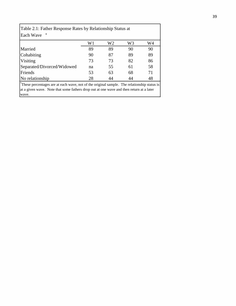
39

W1 W2 W3 W4

Married 89 89 90 90

Cohabiting 90 87 89 89

Visiting 73 73 82 86

Separated/Divorced/Widowed na 55 61 58

Friends 53 63 68 71

No relationship 28 44 44 48

Table 2.1: Father Response Rates by Relationship Status at

Each Wave *

* These percentages are at each wave, not of the original sample. The relationship status is

at a given wave. Note that some fathers drop out at one wave and then return at a later wave.

40

Variables Mean SE

Dependent Variable

Father Involvement ^

3.38 2.17

Independent Variables

Union Status/Transitions

Between Subjects Union Status/Transitions

Continuously Married 0.22 0.41

Continuously Cohabiting 0.07 0.26

Continuously Visiting or Continuously Nonromantic 0.07 0.25

Cohabiting to Married 0.08 0.27

Cohabiting to Not Cohabiting 0.13 0.34

Married to Not Married 0.04 0.20

Visiting/Nonromantic to Married 0.01 0.11

Visiting/Nonromantic to Cohabiting 0.03 0.17

Visiting to Visiting/Nonromantic to Nonromantic 0.13 0.33

Two or Three Transitions 0.22 0.41

Father Characteristics

Father Less than High School 0.31 0.46

Father High School 0.37 0.48

Father Some College 0.21 0.41

Father College 0.11 0.31

Father Age 27.97 6.59

Mother Characteristics

Mother Less than High School 0.33 0.47

Mother High School 0.30 0.46

Mother Some College 0.25 0.43

Mother College 0.12 0.32

Mother Age 25.35

Child Characteristics

Gender of Child 0.52 0.50

Child Low Birth Weight 0.09 0.29

Child Health ^

0.67 0.47

Dyad Characteristics

Race

Both White 0.17 0.37

Both Black 0.44 0.50

Both Hispanic 0.22 0.42

Both Other Race 0.02 0.14

Interracial Couple 0.15 0.35

Table 2.2: Means and SE for All Variables (n = 3,368; Obs. = 31,290)

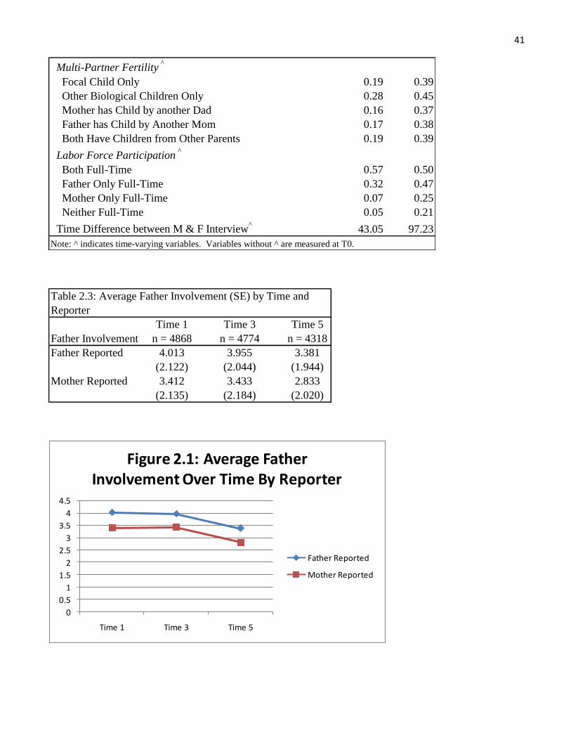
41

Multi-Partner Fertility^

Focal Child Only 0.19 0.39

Other Biological Children Only 0.28 0.45

Mother has Child by another Dad 0.16 0.37

Father has Child by Another Mom 0.17 0.38

Both Have Children from Other Parents 0.19 0.39

Labor Force Participation^

Both Full-Time 0.57 0.50

Father Only Full-Time 0.32 0.47

Mother Only Full-Time 0.07 0.25

Neither Full-Time 0.05 0.21

Time Difference between M & F Interview^

43.05 97.23

Note: ^ indicates time-varying variables. Variables without ^ are measured at T0.

Time 1 Time 3 Time 5

Father Involvement n = 4868 n = 4774 n = 4318

Father Reported 4.013 3.955 3.381

(2.122) (2.044) (1.944)

Mother Reported 3.412 3.433 2.833

(2.135) (2.184) (2.020)

Table 2.3: Average Father Involvement (SE) by Time and

Reporter

0

0.5

1

1.5

2

2.5

3

3.5

4

4.5

Time 1 Time 3 Time 5

Figure 2.1: Average Father Involvement Over Time By Reporter

Father Reported

Mother Reported

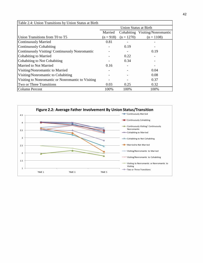
42

Married Cohabiting Visiting/Nonromantic

Union Transitions from T0 to T5 (n = 918) (n = 1270) (n = 1108)

Continuously Married 0.81 - -

Continuously Cohabiting - 0.19 -

Continuously Visiting/ Continuously Nonromantic - - 0.19

Cohabiting to Married - 0.22 -

Cohabiting to Not Cohabiting - 0.34 -

Married to Not Married 0.16 - -

Visiting/Nonromantic to Married - - 0.04

Visiting/Nonromantic to Cohabiting - - 0.08

Visiting to Nonromantic or Nonromantic to Visiting - - 0.37

Two or Three Transitions 0.03 0.25 0.32

Column Percent 100% 100% 100%

Union Status at Birth

Table 2.4: Union Transitions by Union Status at Birth

1

1.5

2

2.5

3

3.5

4

4.5

TIME 1 TIME 3 TIME 5

Figure 2.2: Average Father Involvement By Union Status/TransitionContinuously Married

Continuously Cohabiting

Continuously Visiting/ Continuously Nonromantic

Cohabiting to Married

Cohabiting to Not Cohabiting

Married to Not Married

Visiting/Nonromantic to Married

Visiting/Nonromantic to Cohabiting

Visiting to Nonromantic or Nonromantic to Visiting

Two or Three Transitions

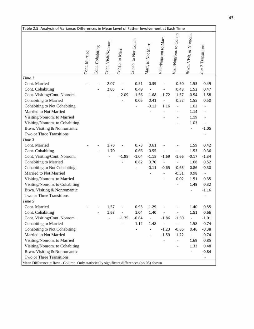
43

Table 2.5: Analysis of Variance: Differences in Mean Level of Father Involvement at Each Time

Cont.

Mar

ried

Cont.

Cohab

itin

g

Cont.

Vis

it/N

onro

m.

Cohab

. to

Mar

r.

Cohab

. to

Not

Cohab

.

Mar

r. t

o N

ot

Mar

r.

Vis

it/N

onro

m t

o M

arr.

Vis

it/N

onro

m. to

Cohab

.

Btw

n. V

isit

. &

Nonro

m.

2 o

r 3 T

ransi

tions

Time 1

Cont. Married - - 2.07 - 0.51 0.39 - 0.50 1.53 0.49

Cont. Cohabiting - 2.05 - 0.49 - - 0.48 1.52 0.47

Cont. Visiting/Cont. Nonrom. - -2.09 -1.56 -1.68 -1.72 -1.57 -0.54 -1.58

Cohabiting to Married - 0.05 0.41 - 0.52 1.55 0.50

Cohabiting to Not Cohabiting - -0.12 1.16 - 1.02 -

Married to Not Married - - - 1.14 -

Visiting/Nonrom. to Married - - 1.19 -

Visiting/Nonrom. to Cohabiting - 1.03 -

Btwn. Visiting & Nonromantic - -1.05

Two or Three Transitions -

Time 3

Cont. Married - - 1.76 - 0.73 0.61 - - 1.59 0.42

Cont. Cohabiting - 1.70 - 0.66 0.55 - - 1.53 0.36

Cont. Visiting/Cont. Nonrom. - -1.85 -1.04 -1.15 -1.69 -1.66 -0.17 -1.34

Cohabiting to Married - 0.82 0.70 - - 1.68 0.52

Cohabiting to Not Cohabiting - -0.11 -0.65 -0.63 0.86 -0.30

Married to Not Married - - -0.51 0.98 -

Visiting/Nonrom. to Married - 0.02 1.51 0.35

Visiting/Nonrom. to Cohabiting - 1.49 0.32

Btwn. Visiting & Nonromantic - -1.16

Two or Three Transitions -

Time 5

Cont. Married - - 1.57 - 0.93 1.29 - - 1.40 0.55

Cont. Cohabiting - 1.68 - 1.04 1.40 - - 1.51 0.66

Cont. Visiting/Cont. Nonrom. - -1.75 -0.64 - -1.86 -1.50 - -1.01

Cohabiting to Married - 1.12 1.48 - - 1.58 0.74

Cohabiting to Not Cohabiting - - -1.23 -0.86 0.46 -0.38

Married to Not Married - -1.59 -1.22 - -0.74

Visiting/Nonrom. to Married - - 1.69 0.85

Visiting/Nonrom. to Cohabiting - 1.33 0.48

Btwn. Visiting & Nonromantic - -0.84

Two or Three Transitions -

Mean Difference = Row - Column. Only statistically significant differences (p<.05) shown.

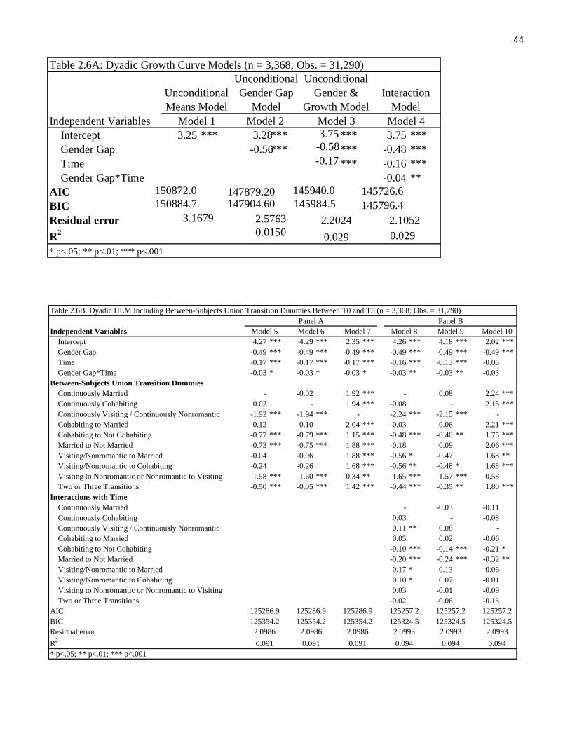
44

Independent Variables

Intercept 4.27 *** 4.29 *** 2.35 *** 4.26 *** 4.18 *** 2.02 ***

Gender Gap -0.49 *** -0.49 *** -0.49 *** -0.49 *** -0.49 *** -0.49 ***

Time -0.17 *** -0.17 *** -0.17 *** -0.16 *** -0.13 *** -0.05

Gender Gap*Time -0.03 * -0.03 * -0.03 * -0.03 ** -0.03 ** -0.03

Between-Subjects Union Transition Dummies

Continuously Married - -0.02 1.92 *** - 0.08 2.24 ***

Continuously Cohabiting 0.02 - 1.94 *** -0.08 - 2.15 ***

Continuously Visiting / Continuously Nonromantic -1.92 *** -1.94 *** - -2.24 *** -2.15 *** -

Cohabiting to Married 0.12 0.10 2.04 *** -0.03 0.06 2.21 ***

Cohabiting to Not Cohabiting -0.77 *** -0.79 *** 1.15 *** -0.48 *** -0.40 ** 1.75 ***

Married to Not Married -0.73 *** -0.75 *** 1.88 *** -0.18 -0.09 2.06 ***

Visiting/Nonromantic to Married -0.04 -0.06 1.88 *** -0.56 * -0.47 1.68 **

Visiting/Nonromantic to Cohabiting -0.24 -0.26 1.68 *** -0.56 ** -0.48 * 1.68 ***

Visiting to Nonromantic or Nonromantic to Visiting -1.58 *** -1.60 *** 0.34 ** -1.65 *** -1.57 *** 0.58

Two or Three Transitions -0.50 *** -0.05 *** 1.42 *** -0.44 *** -0.35 ** 1.80 ***

Interactions with Time

Continuously Married - -0.03 -0.11

Continuously Cohabiting 0.03 - -0.08

Continuously Visiting / Continuously Nonromantic 0.11 ** 0.08 -

Cohabiting to Married 0.05 0.02 -0.06

Cohabiting to Not Cohabiting -0.10 *** -0.14 *** -0.21 *

Married to Not Married -0.20 *** -0.24 *** -0.32 **

Visiting/Nonromantic to Married 0.17 * 0.13 0.06

Visiting/Nonromantic to Cohabiting 0.10 * 0.07 -0.01

Visiting to Nonromantic or Nonromantic to Visiting 0.03 -0.01 -0.09

Two or Three Transitions -0.02 -0.06 -0.13

AIC

BIC

Residual error

R2

0.094

2.0993 2.0993 2.0993

Model 10

125257.2 125257.2 125257.2

125324.5

125286.9

125324.5125324.5

0.091 0.091

Model 8 Model 9

0.094 0.094

125286.9

125354.2

125286.9

125354.2

Table 2.6B: Dyadic HLM Including Between-Subjects Union Transition Dummies Between T0 and T5 (n = 3,368; Obs. = 31,290)

Model 5 Model 6 Model 7

Panel A Panel B

2.0986

125354.2

2.0986 2.0986

* p<.05; ** p<.01; *** p<.001

0.091

Independent Variables

Intercept 3.25 *** 3.28 *** 3.75 *** 3.75 ***

Gender Gap -0.56 *** -0.58 *** -0.48 ***

Time -0.17 *** -0.16 ***

Gender Gap*Time -0.04 **

AIC

BIC

Residual error

R 2

Table 2.6A: Dyadic Growth Curve Models (n = 3,368; Obs. = 31,290)

Unconditional

Means Model

Model 1

Unconditional

Gender Gap

Model

Model 2

Unconditional

Gender &

Growth Model

Model 3

Interaction

Model

Model 4

2.1052 3.1679

147879.20 147904.60

2.5763

150872.0

150884.7

* p<.05; ** p<.01; *** p<.001

0.0150 0.029 0.029

145940.0

145984.5

2.2024

145726.6

145796.4

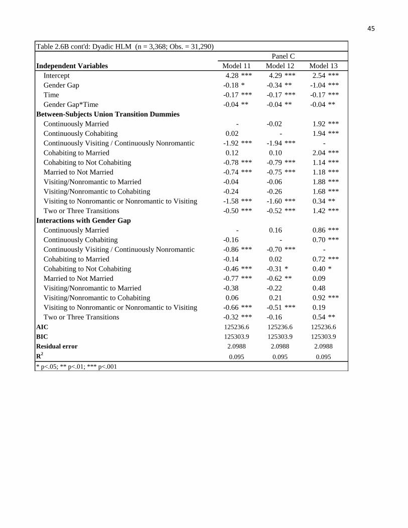
45

Independent Variables

Intercept 4.28 *** 4.29 *** 2.54 ***

Gender Gap -0.18 * -0.34 ** -1.04 ***

Time -0.17 *** -0.17 *** -0.17 ***

Gender Gap*Time -0.04 ** -0.04 ** -0.04 **

Between-Subjects Union Transition Dummies

Continuously Married - -0.02 1.92 ***

Continuously Cohabiting 0.02 - 1.94 ***

Continuously Visiting / Continuously Nonromantic -1.92 *** -1.94 *** -

Cohabiting to Married 0.12 0.10 2.04 ***

Cohabiting to Not Cohabiting -0.78 *** -0.79 *** 1.14 ***

Married to Not Married -0.74 *** -0.75 *** 1.18 ***

Visiting/Nonromantic to Married -0.04 -0.06 1.88 ***

Visiting/Nonromantic to Cohabiting -0.24 -0.26 1.68 ***

Visiting to Nonromantic or Nonromantic to Visiting -1.58 *** -1.60 *** 0.34 **

Two or Three Transitions -0.50 *** -0.52 *** 1.42 ***

Interactions with Gender Gap

Continuously Married - 0.16 0.86 ***

Continuously Cohabiting -0.16 - 0.70 ***

Continuously Visiting / Continuously Nonromantic -0.86 *** -0.70 *** -

Cohabiting to Married -0.14 0.02 0.72 ***

Cohabiting to Not Cohabiting -0.46 *** -0.31 * 0.40 *

Married to Not Married -0.77 *** -0.62 ** 0.09

Visiting/Nonromantic to Married -0.38 -0.22 0.48

Visiting/Nonromantic to Cohabiting 0.06 0.21 0.92 ***

Visiting to Nonromantic or Nonromantic to Visiting -0.66 *** -0.51 *** 0.19

Two or Three Transitions -0.32 *** -0.16 0.54 **

AIC

BIC

Residual error

R2

0.095 0.095

Model 12 Model 13

* p<.05; ** p<.01; *** p<.001

Table 2.6B cont'd: Dyadic HLM (n = 3,368; Obs. = 31,290)

Panel C

0.095

125236.6

2.0988 2.09882.0988

Model 11

125236.6

125303.9125303.9

125236.6

125303.9

46

Independent Variables

Intercept 4.40 *** 4.38 ***

Gender Gap -0.49 *** -0.17 *

Time -0.17 *** -0.16 ***

Gender Gap*Time -0.03 * -0.04 **

Between-Subjects Union Transition Dummies

Continuously Married - -

Continuously Cohabiting 0.25 * 0.15

Continuously Visiting / Continuously Nonromantic -1.71 *** -1.95 ***

Cohabiting to Married 0.28 ** 0.14

Cohabiting to Not Cohabiting -0.57 *** -0.27 *

Married to Not Married -0.61 *** 0.00

Visiting/Nonromantic to Married 0.18 -0.33

Visiting/Nonromantic to Cohabiting -0.03 -0.36

Visiting to Nonromantic or Nonromantic to Visiting -1.35 *** -1.40 ***

Two or Three Transitions -0.30 *** -0.23 *

Interactions with Time

Continuously Married -

Continuously Cohabiting 0.03

Continuously Visiting / Continuously Nonromantic 0.09 *

Cohabiting to Married 0.05

Cohabiting to Not Cohabiting -0.11 ***

Married to Not Married -0.22 ***

Visiting/Nonromantic to Married 0.16 *

Visiting/Nonromantic to Cohabiting 0.11 *

Visiting to Nonromantic or Nonromantic to Visiting 0.02

Two or Three Transitions -0.02

Interactions with Gender Gap

Continuously Married -

Continuously Cohabiting -0.15

Continuously Visiting / Continuously Nonromantic -0.80 ***

Cohabiting to Married -0.14

Cohabiting to Not Cohabiting -0.50 ***

Married to Not Married -0.83 ***

Visiting/Nonromantic to Married -0.35

Visiting/Nonromantic to Cohabiting 0.07

Visiting to Nonromantic or Nonromantic to Visiting -0.67 ***

Two or Three Transitions -0.33 ***

Father Characteristics

Less than High School 0.03 0.03

High School - -

Some College 0.15 * 0.15 *

College 0.40 *** 0.39 ***

Age at Birth -0.01 * -0.01

Table 2.6C: Dyadic HLM Including Between-Subjects Union Transition Dummies

Between T0 and T5 (n = 3,368; Obs. = 31,290)

Model 15 Model 14

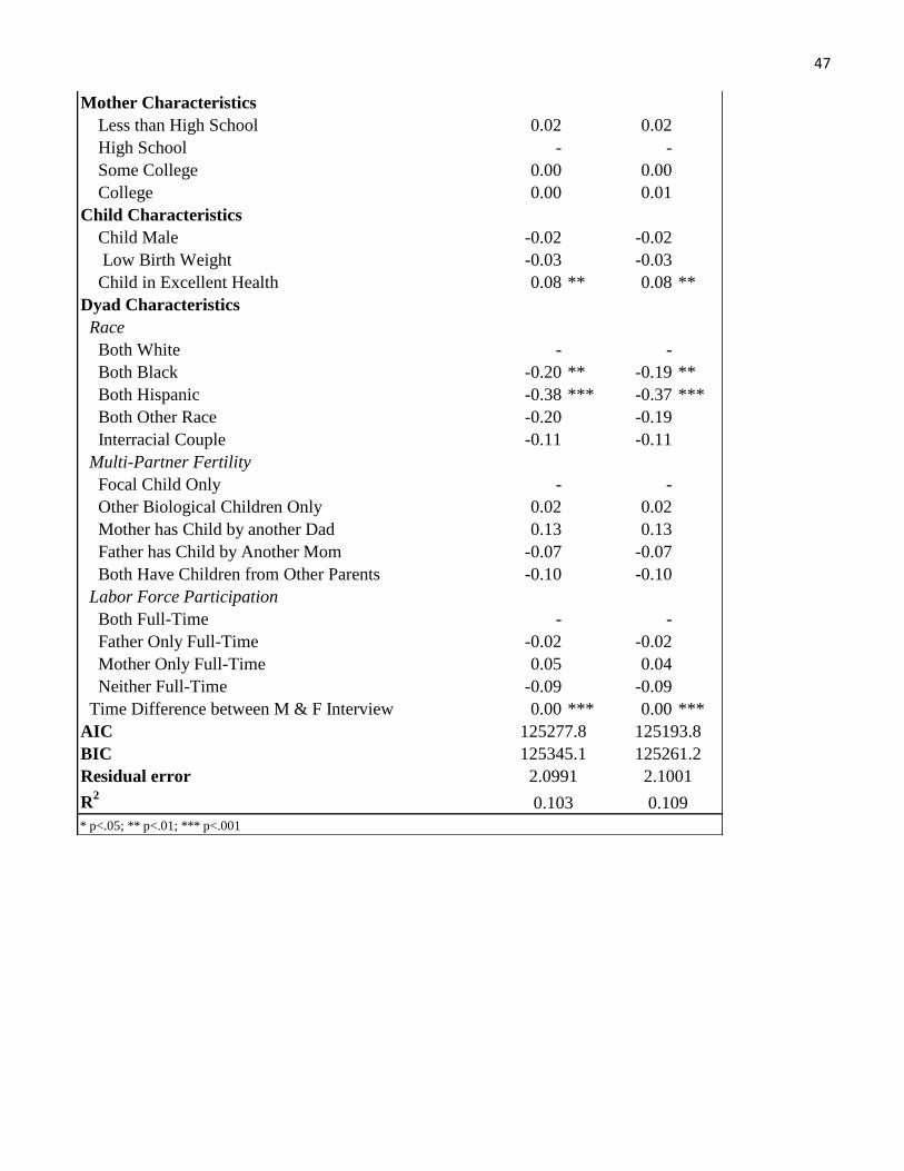
47

Mother Characteristics

Less than High School 0.02 0.02

High School - -

Some College 0.00 0.00

College 0.00 0.01

Child Characteristics

Child Male -0.02 -0.02

Low Birth Weight -0.03 -0.03

Child in Excellent Health 0.08 ** 0.08 **

Dyad Characteristics

Race

Both White - -

Both Black -0.20 ** -0.19 **

Both Hispanic -0.38 *** -0.37 ***

Both Other Race -0.20 -0.19

Interracial Couple -0.11 -0.11

Multi-Partner Fertility

Focal Child Only - -

Other Biological Children Only 0.02 0.02

Mother has Child by another Dad 0.13 0.13

Father has Child by Another Mom -0.07 -0.07

Both Have Children from Other Parents -0.10 -0.10

Labor Force Participation

Both Full-Time - -

Father Only Full-Time -0.02 -0.02

Mother Only Full-Time 0.05 0.04

Neither Full-Time -0.09 -0.09

Time Difference between M & F Interview 0.00 *** 0.00 ***

AIC

BIC

Residual error

R2

* p<.05; ** p<.01; *** p<.001

125193.8

2.0991

0.103 0.109

125261.2

2.1001

125277.8

125345.1