antonije onjia, chemometric approach to the experiment optimization and data evaluation in...

th

U

Chemhe ExpData E

UNIVERSI

Anton

momeperimenEvalua

Ch

Faculty ofBe

ITY OF B

nije E.

etric Apnt Optation inhemist

f Technologelgrade, 201

BELGRAD

Onjia

pproactimizan Anatry

gy and Meta16.

DE

ch to tion anlytical

allurgy

nd l

Antonije E. Onjia CHEMOMETRIC APPROACH TO THE EXPERIMENT OPTIMIZATION AND DATA EVALUATION IN ANALYTICAL CHEMISTRY Reviewers: PhD Snežana Dragović, scientific advisor Vinča Institute of Nuclear Sciences

PhD Slavica Ražić, full professor Faculty of Pharmacy, University of Belgrade

PhD Aleksandra Perić Grujić, full professor Faculty of Technology and Metallurgy, University of Belgrade Publisher: Faculty of Technology and Metallurgy, University of Belgrade Karnegijeva 4 In charge of Publishing: PhD Djordje Janaćković, full professor, dean Editor-in-chief: PhD Karlo Raić, full professor Impression: 200 copies Printed by: Faculty of Technology and Metallurgy, Research and Development Centre of Printing Technology Karnegijeva 4, Belgrade, Serbia

ISBN 978-86-7401-338-0

I

PREFACE

Over the last few decades, the application of chemometric techniques to

all fields in analytical chemistry and particularly to analytical chromatography and spectrometry has increased dramatically. The modern state and the novel application fields of chemometrics, as an interdisciplinary and promising area, have been transferred to legacy to many incoming young and experienced analysts.

Considering chemometrics as an unavoidable part of experimental design and data interpretation in personal work, the idea of writing this monograph, as helpful supplement to common knowledge of chemometrics in analytical chemistry, has originated.

It has been about 35 years since the first chemometric handbooks were printed. Nowadays, everybody has to acknowledge a huge significance in analytical chemistry and many related disciplines. The chemometric concept in the most of these books has been presented to the readers in a manner that does not assume a very good background in statistics or matrix algebra. Today handbooks that are being printed present a huge effort to explain and clarify the state of the art in chemometrics, so they can be highly recommended to anyone working in this field.

This monograph represents the modest contribution to the modern aspects of chemometrics, especially underlining the most popular methods and scopes stuffed with comprehensive and useful examples of their practical applications in analytical chemistry. Such monograph could be figured as useful reading to a wide range of analytical chemistry practitioners who are not new in this field but who simply need to have some specific aspects of chemometrics all along in their everyday practice. Such aspects of this intricate and complex matter are herein described in detail and designed to be easily reached and understood.

Theoretical basics are explained and supported by practical examples in a style that makes the material accessible to a broad audience of analytical chemists. After all, this monograph certainly has been derived from a long-term practical and theoretical work in this field and experience that has been gathered on that road.

II

The monograph covers 12 chemometric fields of interest divided into 5 main chapters. Every chapter can be studied separately since it has been written as a stand-along piece of text. This way, the reader could study every chapter as a unity. Each topic is supported by basic theory, followed by several representative examples. Some information are repeated in different places with similar or different purpose so this hopefully could help the reader to recall or rethink a topic in a different way.

Dr Antonije Onjia

III

Contents

1. INTRODUCTION ............................................................................... 1

2. OPTIMIZATION OF EXPERIMENT .............................................. 11

2.1. Simultaneous Approach .............................................................. 12

2.1.1. Experimental design ............................................................ 12

2.1.2. Artificial neural network ..................................................... 30

2.2. Sequential Approach ................................................................... 44

2.2.1. Simplex ................................................................................ 44

3. SIGNAL PROCESSING ................................................................... 55

3.1. Multivariate Calibration ............................................................. 61

4. DATA EVALUATION ..................................................................... 73

4.1. Unsupervised Pattern Recognition ............................................. 75

4.1.1. Principal component and cluster analysis ........................... 76

4.1.2. Kohonen artificial neural network ....................................... 89

4.2. Supervised Pattern Recognition .................................................. 96

4.2.1. Discriminant analysis .......................................................... 96

4.2.2. K-nearest neighbor ............................................................ 100

4.2.3. Soft independent modeling of class analogy ...................... 107

4.2.4. Feed forward artificial neural network ............................. 112

4.2.5. Multiway pattern recognition (Tucker, Parafac, Unfolding) ............................................ 121

5. SUMMARY AND OUTLOOK ....................................................... 131

6. REFERENCES ................................................................................ 135

1

1. INTRODUCTION

As officially defined, chemometrics is a chemical discipline that uses mathematics, statistics, and formal logic to design or to select optimal experimental procedures, to provide the most relevant chemical information by analyzing chemical data, and to obtain knowledge about chemical systems. Typical applications of chemometric methods are the development of quantitative structure activity relationships or the evaluation of analytical chemical data.

The Swede, Svante Wold in 1971 introduced the term “kemometri” in Swedish and soon English equivalent “chemometrics” entered the world of science with the help of the American scientist Bruce Kowalski. However, the first appearance of this term varied from field to field. The International Chemometrics Society was established in 1974. In 1986 and 1987, two journals were launched, “Chemometrics and Intelligent Laboratory Systems” (Elsevier) and “Journal of Chemometrics” (Wiley). They promoted equipment intellectualization and offered new methods for the construction of novel and high-dimensional hyphenated equipment.

The education of analytical chemists in mathematics and statistics does not offer the expected outcomes and skills in their understanding of the processes. Therefore, one of the initial aims of chemometrics was to make complicated mathematical methods understandable to practitioners of various backgrounds.

Apart from the statistical-mathematical methods, the topic of chemometrics is also related to the problems of the computer-based laboratory, to the methods of handling chemical or spectroscopic databases and to the methods of artificial intelligence.

Since 1990, there has been an ever-growing increase in the use of chemometrics in various fields of analytical science and practice. The ready availability of packaged software has certainly speeded up the procedure. Very large amount of data had suddenly appeared, especially in biological and medical analytical applications, and eventually imposed a need for the methods for the resolution and pattern recognition of those data using multivariate methods.

2 A. ONJIA - Chemometric approach to the experiment optimization and data ...

Wherever a bunch of analytical data is acquired and where experiment should be conducted in the most optimized form, chemometrics found its place and adapted to the matter. For instance, commonly used chemometric techniques in herbal drug standardization are principal component analysis (PCA), linear discriminate analysis (LDA), spectral correlative chromatography (SCC), information theory (IT), local least square (LLS), heuristic evolving latent projections (HELP) and orthogonal projection analysis1 (OPA).

Applications of chemometrics in analytical electrochemistry include many chemometric methods such as multiple linear regression (MLR), Kalman filter (KF), principal component analysis (PCA) and principal component regression (PCR), evolving factor analysis (EFA), partial least squares (PLS), Fourier transform (FT) and artificial neural networks (ANNs). These methods have been applied in electrochemistry to facilitate parameter estimation, optimization, signal processing, and pattern recognition2. Thus, it can be seen that the application of chemometrics in just these two fields is very colorful and complex.

Three critical properties of the measurement process include its chemical (stoichiometry, mass balance, chemical equilibria, kinetics), physical (temperature, energy transfer, phase transitions), and statistical properties (sources of errors in the measurement process, control of interfering factors, calibration of response signals).

Deep understanding and control of these three critical properties of a chemical measurement are essential in providing a reliable information about the system. If any of these three properties is missing, the measuring process will be unstable and will fail to provide reliable results. The role of chemometrics is to address the statistical properties.

Some major application areas of chemometrics include (1) calibration, validation, and significance testing; (2) optimization of chemical measurements and experimental procedures; and (3) the extraction of the maximum amount of chemical information from analytical data.

Before the beginning of the data collection, one or more hypotheses about the problem that one have to deal with should be established. Analysis of the results is very important. One of the desirable outcomes of a structured approach is that one may find that some variables in a technique have little or no influence on the results obtained and could be omitted.

In the simplest case, data are single numerical results from a procedure or assay, for instance, concentration of cadmium in the sample of soil. However, in modern analytical practice more complex data are encountered such as spectrum, chromatogram etc. This led to multivariate calibration models

INTRODUCTION 3

in chemometrics since the results from a calibration needed to be validated rather than just a single value recorded. Therefore, the quality of the calibration and the robustness needs to be tested. In addition, the quality of any model is very dependent on the test specimens used to standardize it, which make sampling very important as well.

Estimate of the error or uncertainty in the measurement is essential in dealing with numerical measurement. Therefore, estimating the error or degree of uncertainty for each measurement should be everyday routine. But, if a measurement seems rather high compared with the rest of the measurements in the set, statistics must always relate the results from the given statistical test to the data to which the data has been applied, and relate the results to given knowledge of the measurement.

In measurement process, great attention should be devoted to errors. The largest error in the data set will always dominate small errors. For instance, large error in a reference method of solution standardization occurs during measuring mass of the substance on the technical balance with a precision to one hundredth of the gram, which makes standard solution unsuitable for analytical chemistry. Statistics should not be misused to grant sense to poor data from the poor experiment since the results of any statistical test are only as good as the data to which they are applied3. Common types of errors in measuring are gross error, systematic, and random error. Gross errors are defined as major errors induced by power failure of the instrument, mislabeling or contamination of the specimen etc. When these errors are detected, the experiment must be repeated.

Systematic error (bias) can be easily discovered since it arises from imperfections in an experimental procedure that leads to a bias in the results. They usually originate from a poorly calibrated instrument or contaminated water supply (laboratory bias) or could be detected by using standard reference materials (method bias). Bias is defined as:

0e x μ μ μ= − + − (1.1)

where x is the analytical measurements of a quantity, µ is the true mean (or population mean), and µo the true or correct value for that measured analyte obtained from an infinite number of measurements. Random errors are the errors that experimenter often is not aware of. They arise, for instance, as electrical noise of the measuring instrument and produces results that are spread about the average value. Random errors affect the precision or reproducibility of the results.


It is said that a set of measurements made in succession in the same laboratory using the same equipment is performed within run, which is opposite to between run experiments where measurements are made at over longer time period, possibly in different laboratories and under different circumstances. The first notion is tested with repeatability, while the latter is tested with reproducibility.

Experiment with a small systematic error is said to be accurate, while that with a small random error is said to be precise. Accuracy is defined as ability of the measured results to match the true value for the data while precision is the variations between variates. In everyday practice, it is more common to be more concerned with the precision than the accuracy. The main problem is that a true value is often not known in experimental science.

Figure 1.1. Representation of precision and accuracy as shots on the target.

Mean, variance, and standard deviation are useful exploratory statistic measures that should be calculated to consider the quality of a dataset4.

The arithmetic mean is a measure of the average or central tendency of a set of data and is usually denoted by the symbol ̅. The value for the mean is calculated by summing the data and then dividing this sum by the number of values (n).

_ix

xn

= (1.2)

The variance in the data, a measure of the spread of a set of data, is related to the precision of the data. For example, the larger the variance, the larger the spread of data while the precision is lower. It is defined as:

INTRODUCTION 5

_2

2( )ix x

sn

−= (1.3)

The standard deviation (s) of a set of data is the square root of the variance. For large values of n, the population standard deviation is calculated using the formula:

_2( )ix x

sn

−= (1.4)

If the standard deviation is to be estimated from a small set of data, it is more appropriate to calculate the sample standard deviation:

_2( )

1ix x

sn

∧ −=

− (1.5)

The relative standard deviation (named also the coefficient of variation) is a dimensionless quantity defined as:

sRSD

x= (1.6)

Assuming that the data are normally distributed in some measurement allows us to use the well-understood mathematical distribution known as the normal or Gaussian error distribution where we can compare the collected data with an acknowledged statistical model to determine the precision of the data.

Although the standard deviation gives a measure of the spread of a set of results about the mean value, it does not indicate the way in which the results are distributed. Therefore, a large number of results is needed to characterize the distribution. The spread of a large number of collected data points will be affected by the random errors in the measurement and this will cause the data to follow the normal distribution. The mathematical model used to describe the normal or Gaussian distribution is:

2 2exp ( ) / 2

2

xy

μ σ

σ π

− − = (1.7)


where µ is the true mean (or population mean), x is the measured data, and σ is the true standard deviation (population standard deviation). For a normal distribution with mean μ and standard deviation σ:

- approximately 68% of the population values lie within ±1σ of the mean;

- approximately 95% of population values lie within ±2σ of the mean; - approximately 99.7% of population values lie within ±3σ of the mean. Normal distribution is represented in Figure 1.2. The curve is

symmetrical about μ and the greater the value of σ the greater the spread of the curve. For a normal distribution with known mean, μ, and standard deviation, σ, the exact proportion of values that lie within any interval can be found from tables, if the values are first standardized to give z-values5. This is done by expressing any value of x in terms of its deviation from the mean in units of the standard deviation, σ, in order to obtain standardized normal variable:

( )xz

μσ−= (1.8)

Figure 1.2. Normal distributions with the same mean but different values of the standard deviation.

The confidence interval is the range within which it is reasonable to assume that a true value lies, while the confidence limits are the extreme values of this range3.

Significance test is a statistical test employed to decide whether the difference between the measured values and standard or reference values can be

INTRODUCTION 7

attributable to random errors. It is possible to visually estimate if the results from two methods produce similar results, but without the use of a statistical test, a judgment on this approach is purely empirical.

Therefore, significance test is used to confirm if there is no significant difference between the two methods used since it enables quantification of the difference or similarity between the methods. Significance testing is divided to testing for accuracy by using the student t-test and to testing for precision by using the F-test.

The F-test is a powerful statistical test which is defined as a simple ratio of two sample variances. This is given in the following equation:

22

21

s

sF = (1.9)

where s1 and s2 are variances from the first and the second set of data, respectively. F value must be ≥ 1 so the sets must be arranged properly. In performing a significance test, we test the truth of a hypothesis, known as the null hypothesis. If there is no statistically significant difference between the two variances (the null hypothesis is retained), then the calculated F value will approach 1. The test can be used in two ways; to test for a significant difference in the variances of the two samples or to test whether the variance is significantly higher or lower for either of the two data3.

The student t-test is employed to estimate whether an experimental mean ( ̅) differs significantly from the true value of the mean, µ. Therefore, it deals with the problems associated with inference based on "small" samples: the calculated mean ( ̅) and standard deviation (σ) may accidentally deviate from the "real" mean and standard deviation6. In the case where the deviation between the known and the experimental values is considered to be caused by the random errors, the method can be used to assess accuracy.

Alternatively, the deviation becomes a measure of the systematic error or bias. The approach to accuracy is limited to where test objects can be compared with reference materials. The numerical outcome of the t-test to be compared with the tabulated critical values of t is calculated from the experimental results as given here:

/

xt

n

μσ

−= (1.10)


If the absolute value of t exceeds the critical value (determined by the required confidence limit and the number of degrees of freedom) then the null hypothesis is rejected3.

A one-tailed test (directional hypothesis) and two-tailed test (a non directional hypothesis) are tests of significance to determine if there is a relationship between the variables in one and in either direction, respectively. A two-tailed test is used if deviations of the estimated parameter in either direction from some benchmark value are considered theoretically possible while a one-tailed test is used if only deviations in one direction are considered possible.

One-tailed tests are used for asymmetric distributions that have a single tail such as the chi-squared distribution or for one side of a distribution that has two tails, such as the normal distribution. Two-tailed tests are only applicable when there are two tails, such as in the normal distribution, and correspond to considering either direction significant.

When more than two methods or sample treatments should be compared, two possible sources of variation must be considered, those associated with systematic errors and those arising from random errors.

Analysis of variance (ANOVA) is extremely powerful statistical technique, which can be used to separate and estimate the different causes of variation and to evaluate both systematic and random errors7. It tests the hypothesis that the means of two or more populations are equal. Therefore, it assesses the importance of one or more factors by comparing the response variable means at the different factor levels.

The null hypothesis states that all factor level means are equal while the alternative hypothesis states that at least one is different. A continuous response variable and at least one categorical factor with two or more levels should be considered in ANOVA. It requires data from approximately normally distributed populations with equal variances between factor levels. Practical use of ANOVA covers, for instance, interlaboratory trials or method comparison (when several laboratories and methods are involved).

Homoscedastic results have the different mean values of the samples (treatments) and the same variance, while heteroscedastic results have the different variance. In the case of homoscedastic variation, the variance is constant with increasing mean response, whereas with heteroscedastic variation the variance increases with the mean response.

ANOVA is sensitive to heteroscedasticity because it attempts to use a comparison of the estimates of variance from different sources to infer whether the treatments have a significant effect.

INTRODUCTION 9

There are issues that can influence the outcome of any statistical test since the results used are affected by the quality of the analyzed data. Therefore, it is also important to estimate the quality of the input data to ensure that it is free from errors.

Outliers are commonly one of the sources of such errors. An outlier is an observation point that is distant from other observations. The inclusion of bad data in any statistical calculation can lead to great mistakes in estimation. In order to avoid including outliers in the data one should have sufficient replicates for all samples (that is difficult to achieve in practice).

Experimental outliers are outliers in the analytical measurement or samples, while also source of error might be in the reference value. Anyhow, since one cannot simply remove disputable data, the whole pool of data must be systematically scrutinized to ensure that any suspected outliers can be proven to lie outside the expected range for that data3.

To conclude, stragglers and outliers are two types of “extreme values” which can exist in any experimentally measured results. They differ in confidence level required to distinguish between them. While stragglers fall within the 95-99% of the confidence levels, outliers are detected at >99% confidence limit. One should bear in mind that suspicious “very extreme” data points could in fact be correct, while one in every 20 samples examined is typically classified incorrectly.

11

2. OPTIMIZATION OF EXPERIMENT

The optimization of experiments is a tool used to find optimum conditions for an experiment systematically. It is not hard to see that if experiments were performed with no rule, the results obtained would hardly make sense. Hence, plan of the experiments in such a way that the meaningful and useful information are obtained is necessary for a start.

When the goal of the research is clearly known, following issues should be addressed: what do we know about the system that we study, what is unknown, what do we need to investigate, which experimental variables are to be determined, which responses can be measured etc.? When all of these questions are borne in mind all the time, we are on the right way to acquire maximum information from a minimum of experiments.

Optimum response of experiment is provided when separate methods are employed to determine the combination of factor levels affecting the results of that experiment. Defining the optimum response in given analytical procedure is of critical importance. Sometimes it might refer to maximum response signal (for example, the largest possible absorbance, current, emission intensity, etc.). On the other hand, the optimum response of some experiment may imply the maximum signal to noise or signal to background ratios, the best resolution in separation methods, or even a minimum response (for instance, when the removal of an interfering signal is being studied).

Quality of good optimization method assumes two things: optimization produces a set of experimental conditions that provides the optimum or near optimum response; and is done so with the smallest possible number of trial experimental steps.

Generally, in optimization of experiments two approaches are possible: a single approach in which the several parameters are estimated simultaneously from one optimal experiment, and a sequential approach where in sequential order, several optimal experiments are implemented which focus on a few parameters, and (nominal) parameter estimates are updated intermediately.


2.1. Simultaneous approach

2.1.1. Experimental design

If someone wants to conceive experimental design properly, he/she should identify the factors that may affect the result of an experiment, organize the experiment so that the effects of uncontrolled factors are minimized, and use statistical analysis to separate and evaluate the effects of the various factors involved. Exact purpose of the experiment must be known before any steps of experimental design are made. It is always a case in practice that large number of factors are involved in every experiment (e.g. measuring, determination, optimization) so they unavoidably make the whole process rather complicated.

Sometimes the experiment is a bit easier if someone has information about the similar experiment previously carried out. There is a great deal of literature on the factors studied by other experimenters aiming for the same result and it is reasonable to consider efforts and works of the others. During this, the other problem occurs since it is very difficult to reproduce experiments in one laboratory exactly in the same manner as in another. Many uncontrolled factors, such as reagent or solvent purity, humidity, temperature, different instruments with different properties etc. may cause such an inequity in vide range of experiments. That is why quite complex experimental designs are always necessary8.

Let us define some of popular terms that are very important for experimental design. Experimental domain is the experimental “area” that is being investigated. It is defined by the variation of the experimental variables. Factors are experimental variables that can be changed independently of each other (similar to independent variables). Continuous variables are independent variables that can be changed continuously. Discrete variables are independent variables that are changed step-wise. Responses are the measured value of the results from experiments, while residual is defined as a difference between the calculated and the experimental result.

As a fact, we will state that the outcome of an experiment is dependent on the experimental conditions. This means that the result can be described as a function based on the experimental variables:

( )y f x= (2.1)

The function f(x) is approximated by a polynomial function and represents a good description of the relationship between the experimental variables and the responses within a limited experimental domain. Three types

OPTIMIZATION OF EXPERIMENT 13

of polynomial models will be discussed and exemplified with two variables, x1 and x2. The simplest polynomial model contains only linear terms and describes only the linear relationship between the experimental variables and the responses. The two variables x1 and x2 are for a linear model expressed as:

0 1 1 2 2y b b x b x residual= + + + (2.2)

Additional terms that describe the interaction between different experimental variables represent the next level of polynomial models. If we apply this, a second order interaction model would be represented by:

0 1 1 2 2 12 1 2y b b x b x b x x residual= + + + + (2.3)

The two models above are mainly used to investigate the experimental system, for instance, with screening studies, robustness tests or similar. If we want to determine an optimum maximum or minimum, quadratic terms have to be introduced in the model. In such a way, it is possible to determine non-linear relationships between the experimental variables and responses. The polynomial function below describes a quadratic model with two variables:

2 20 1 1 2 2 11 1 12 2 12 1 2y b b x b x b x b x b x x residual= + + + + + + (2.4)

The polynomial functions described above contain a number of unknown parameters (b0, b1, b2, etc) that are to be determined. Certainly, for the different models different types of experimental designs are needed.

Several experimental variables or factors may influence the result. The main role of screening of the experiment is to determine the experimental variables and interactions that have significant influence on the result, measured in one or several responses.

That is why we have to specify the problem as the critical thing, review the whole procedure different moments, critical steps, raw material, equipment, and the very problem should be viewed from different angles. In addition, attention should be devoted to which response can be measured and which source of errors can be assumed. Is it possible to follow the change in responses in with the changing time?

In addition, one should know which experimental variables are possible to study. Variables should be analyzed and labeled as important or probably unimportant. Then, experimental domain should be selected and it should be tested if all the variables are of some interest. Which interaction effects can we expect? Which variables are probably not interacting? This gives a list of possible responses, experimental variables and potential interaction effects. This


is all very important. Devoted time to this matter and labor to planning of any experiment is paid back with the huge benefit in the end.

First thing to start with is to select the variables to investigate. When you select the variables, you should know the variables that you will not investigate as well and keep them at a fixed level in all experiments included in the experimental design. It is better to include a few extra variables in the first screening and then add one variable later. In addition, one should consider how the different variables should be defined.

It is sometimes possible to lower the number of experiments needed, in order to achieve the important information, just by redefining the original variables. For instance, for experiments where various concentrations of the solutions are involved, instead of that concentrations relative ratios of concentrations might be used in order to decrease the number of variables.

At the end, when the variables have been established, experimental design should be chosen to estimate the influence of the different variables on the result. Linear or second order interaction models are very frequent in linear screening studies (e.g. factorial or fractional factorial designs). Factorial design is limited to the determination of linear influence of the variables, while fractional design allows for interaction terms between variables to be evaluated as well9.

For instance, if you want to investigate a chemical reaction, then, proportion of solvent, catalyst concentration, temperature, pH, and stirring rate are crucial factors to consider and analyze. Optimization is the process of finding the most suitable factor levels and it is very applicable concept in modern instrumental analytical chemistry, for instance in chromatography. Fractional factorial, Taguchi and Plackett–Burman designs are representatives of saving time designs that are frequently used in industrial processes. Central composite design and calibration designs are used in quantitative modeling.

An experiment where the response variable is measured for all possible combinations of the chosen factor levels is known as a complete factorial design. This type of design is quite different from an approach which is perhaps more obvious, a one-at-a-time design, in which the effect of changing the level of a single factor on the response, with all the other factors held at constant levels, is investigated for each factor in turn. There are two reasons for preferring a factorial design to a one-at-a-time approach. The fundamental reason is that a suitable factorial design can detect and estimate the interactions between the factors, while a one-at-a-time methodology cannot. Secondly, even if interactions are absent, a factorial design needs fewer measurements than the one-at-a-time approach to give the same precision5.


In order to minimize the need for numerous experiments, in many factorial designs each factor is studied at just two levels, (“low” and “high”). These designs are known as screening designs. Mainly the experience and knowledge of the experimenter and the physical constraints of the system determine the exact choice of levels.

For a qualitative variable “high” and “low” refer to a pair of different conditions, such as the presence or absence of a catalyst, the use of mechanical or magnetic stirring, or taking the sample in powdered or granular form. Obvious problem in using a factorial design is that for factors, which are continuous variables, the observed effect depends on the high and low levels used. Let us examine the case with three factors: A, B and C. This means that there are 23=8 possible combinations of factor levels, as shown in Table 2.1.

A plus sign denotes that the factor is at the high while, a minus sign that it is at the low level. In three-level designs, the symbols +1, 0 and -1 are often used to denote the levels. The first column gives a notation often used to describe the combinations, where the presence of the appropriate lower case letter indicates that the factor is at the high level and its absence that the factor is at the low level. The number 1 is used to indicate that all factors are at the low level.

In a contrast, for a given number of factors, fractional factorial designs use one-half, one-quarter, one-eighth, etc. of the number of experiments that would be used in the complete factorial design. The individual experiments in the fractional design must be carefully chosen to ensure that they give the maximum information.

Table 2.1. Complete factorial design for three factors

Combination A B C Response 1 - - - y1 a + - - y2

b - + - y3 c - - + y4

bc - + + y5 ac + - + y6 ab + + - y7 abc + + + y8

The theory of D-optimal designs is the most extensively developed, and

consequently there is quite a long list of works devoted to the construction of practical and realizable D-optimal designs, which include Fedorov’s Algorithm,


Wynn-Mitchell and van Schalkwyk Algorithms, DETMAX Algorithm, The MD Galil and Kiefer’s Algorithm and many sequential composite D-optimal designs3.

In the following example, experimental parameters were optimized by fractional factorial design and response surface methodology in the case of determination of total halogens in coal with oxygen bomb combustion followed by ion chromatography10. Influence of six variables (oxygen pressure, catalyst, absorption solution, reduction reagent, bomb cooling time, and a combustion aid) were examined to establish an accurate, precise, and reliable method for determination of total halogens in coal.

Response surface methodology was conducted to further refine the results obtained by fractional factorial design and to define parameters for the procedure. The accuracy and precision of combustion with ion chromatography were evaluated by the use of two certified reference materials and by fortified in-house coal standards.

The 26-2 fractional factorial design consisted of nineteen experimental runs including three replicates of the central point. The investigated factors were tested at low and high level from the matrix using Minitab software ver. 13. In order to ensure that uncontrolled factors did not affect the results, the experiments were performed randomly.

The data were graphically displayed using Pareto charts (Figure 2.1.) to establish the relationship between investigated factors and total halogen determination. Estimated effects and regression coefficients, presented in Table 2.2., and analysis of variance (ANOVA) were used to determine the effects of factors upon the total halogen determination. The standard error for each estimated regression coefficient was 7.66 percent5.

For the center point, the standard error for estimated regression coefficient was 19.29 percent. Changes in the level of a factor influence the system response, which represents the effect of the factor. The Pareto chart compares absolute values and the significance of effects.

OPTIMIZATIO

Tsolution. based on the catalynegative i

Figure 2halogen

perce(B) cata

ON OF EXPERIME

The most signThe relativthe factor ef

yst and typeinfluences on

2.1. Pareto cns by combusent confidencalyst/coal ma

(E) bomb

ENT

nificant factoe magnitudeffect and core of absorptn halogen rel

chart of the sstion ion chroce interval. Fass ratio, (C)cooling time

ors were the es of the prrresponding tion solutionlease during

standardizedomatographyFactor abbre) absorption e, and (F) co

catalyst and rocess variabp-value. Hig

n indicated tcoal combus

d effects for dy. The vertic

eviations: (A)solution, (D)mbustion aid

the type of ables were dgh negative ethat these fastion5.

determinational line define) oxygen pres) hydrogen pd. (Ref. 10)

17

absorption determined effects for actors had

n of total es the 95

essure, peroxide,


Table 2.2. Estimated effects and regression coefficients for fractional factorial design (Ref. 10)

Term Effect Coefficient T-value p-value Constant 333.06 43.45 0.001 Oxygen pressure 26.13 13.06 1.70 0.231 Catalyst/coal ratio -113.63 -56.81 -7.41 0.018 Absorption solution -95.37 -47.69 -6.22 0.025 H2O2 -18.13 -9.06 -1.18 0.359 Cooling time 7.88 3.94 0.51 0.659 Combustion aid 38.63 19.31 2.52 0.128 Oxygen pressure*Catalyst/coal ratio

-8.13 -4.06 -0.53 0.649

Oxygen pressure*Absorption solution

-2.38 -1.19 -0.15 0.891

Oxygen pressure*Hydrogen peroxide

18.88 9.44 1.23 0.343

Oxygen pressure*Cooling time 26.37 13.19 1.72 0.228 Oxygen pressure*Combustion aid

-42.87 -21.44 -2.80 0.108

Catalyst/coal ratio* Hydrogen peroxide

20.62 10.31 1.35 0.311

Catalyst/coal ratio*Combustion aid

18.38 9.19 1.20 0.353

Oxygen pressure*Catalyst/coal ratio* Hydrogen peroxide

14.13 7.06 0.92 0.454

Oxygen pressure*Catalyst/coal ratio*Combustion aid

17.38 8.69 1.13 0.375

Central point 4.60 0.24 0.834 Analysis of variance (ANOVA) provided information on two- and

three-way interactions between investigated factors. So, by comparing the estimated p-values and established criterion (p=0.05), there were no interactions that significantly influence the determination of total halogens. The only two-way interaction was observed between oxygen pressure and combustion aid and showed that at low oxygen pressure (1.5 mega Pa), the concentration of halogens increased with the volume of mineral oil5.


Table 2.3. Analysis of variance (ANOVA) for response surface model (coded units) (Ref. 10)

Source of variation

Degrees of

freedom

Sequential sum

of squares

Adjusted sum

of squares

Adjusted mean

of squaresF-value p-value

Regression 5 1399.89 1399.89 279.979 20.90 0.000 Linear 2 546.25 546.25 273.127 20.39 0.001 Square 2 670.04 670.04 335.018 25.01 0.001 Interaction 1 183.60 183.60 183.603 13.71 0.008 Residual error 7 93.78 93.78 13.397 Lack-of-fit 3 58.98 58.98 19.659 2.26 0.224 Pure error 4 34.80 34.80 8.700 Total 12 1493.67

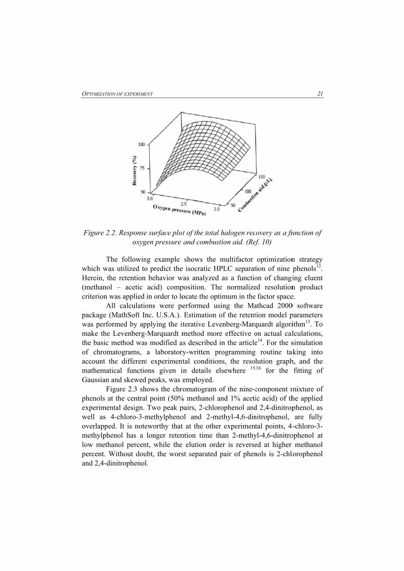
The main objective of response surface methodology is to determine the

optimal operational conditions or to determine the area that meets the operating specification. The difference between a response surface equation and the equation for a factorial design is the addition of quadratic terms that allow model curvature in the response, making them useful for understanding how changes of input factors influence the response of interest, finding the levels of input factors that optimize the response, and selecting the operating conditions to meet the specifications11.

Central composite design is a response surface methodology that is often used when the design calls for sequential experimentation because this approach may incorporate information from a properly planned factorial experiment5.

In order to optimize the total halogens extracted from coal, the experiment was conducted with total halogen recovery as the response variable in the central composite design. Total halogen recovery was calculated as the ratio of the measured and certified values. The pressure and combustion aid were chosen as independent factors for additional experiments. The low, middle, and high levels of each factor were employed with five central points resulting in a matrix of thirteen experiments obtained by statistical software.

The influence of oxygen as a fuel for coal combustion was investigated at 2, 2.5, and 3 mega Pa. Since the combustion aid affected halogen release from coal during combustion according to screening experiments, this parameter was investigated by the addition of 50, 100, or 150 microliters5.


According to the results obtained from the fractional factorial design, it was concluded that catalyst and alkaline solution negatively influenced the total halogen determination. Since the change of the concentration of H2O2 as reducing agent from low to medium level had no effect, its concentration was employed at 0.5 wt. percent. Sufficient dissolution of gases was achieved after fifteen minutes of cooling the oxygen bomb5.

Response surface methodology consists of a group of mathematical and statistical techniques that are based on the fitting of empirical models to the experimental data obtained in relation to the experimental design. Table 2.4 summarizes the estimated regression coefficients from linear, square, and interaction models. The combustion aid, as well as oxygen pressure, and oxygen pressure combustion aid interactions, according to p-values, were statistically significant on the total halogen determination.

The coefficient of variation was R2=93.72%, indicates a high degree of correlation between the response variable and independent factors and a high degree of fitting. The results shown in Table 2.3 (ANOVA) and response surface plot shown on figure 2.2. confirmed that the combustion aid improved the recovery and the accuracy of halogen determination in coal. The volume of the combustion aid was set at 150 microliters and the oxygen pressure at 2.5 mega Pascals.

Table 2.4. Estimated regression coefficients for response surface design (Ref. 10)

Term Coefficient Standard error

of the coefficient p-value

Constant 87.231 1.520 0.000 Oxygen pressure 1.433 1.494 0.369 Combustion aid 9.433 1.494 0.000

Oxygen pressure*Oxygen pressure -14.859 2.202 0.000 Combustion aid*Combustion aid 1.341 2.202 0.562 Oxygen pressure*Combustion aid -6.775 1.830 0.008

OPTIMIZATIO

Figure 2

Twhich waHerein, th(methanocriterion w

Apackage (was perfomake thethe basic of chromaccount tmathematGaussian

Fphenols aexperimewell as overlappemethylphlow methpercent. Wand 2,4-d

ON OF EXPERIME

.2. Responseoxyg

The followinas utilized tohe retention

ol – acetic was applied

All calculatio(MathSoft Inormed by ape Levenberg-

method wasmatograms, the differenttical functioand skewed

Figure 2.3 shat the centralntal design. 4-chloro-3-m

ed. It is notehenol has a hanol percenWithout dou

dinitrophenol

ENT

e surface plotgen pressure

ng example o predict the

behavior wacid) compin order to loons were penc. U.S.A.). pplying the it-Marquardt ms modified aa laboratoryt experimentons given i

peaks, was ehows the chrol point (50%Two peak p

methylphenoeworthy thatlonger reten

nt, while the ubt, the worsl.

t of the total and combus

shows the e isocratic HP

was analyzed position. Thocate the opterformed usEstimation terative Levmethod mor

as described y-written prtal conditionin details eemployed. omatogram

% methanol apairs, 2-chlorol and 2-met at the otherntion time th elution ordst separated

halogen rection aid. (Ref

multifactor PLC separatas a functio

e normalizetimum in thesing the Maof the retentenberg-Marqe effective oin the articlerogramming ns, the resolsewhere 15,

of the nine-cand 1% acetirophenol andethyl-4,6-dinr experimenthan 2-methy

der is reversepair of phen

overy as a fuef. 10)

optimizationtion of nine on of changied resolution

factor spaceathcad 2000tion model pquardt algorion actual cale14. For the s

routine talution graph,16 for the

component mic acid) of thd 2,4-dinitropnitrophenol, tal points, 4

yl-4,6-dinitroed at higher nols is 2-chl

21

function of

n strategy phenols12. ing eluent n product e. 0 software parameters ithm13. To lculations, simulation

aking into h, and the fitting of

mixture of he applied phenol, as are fully

4-chloro-3-ophenol at

methanol lorophenol


Figure 2.3. Chromatogram of nine phenols at 50% methanol and 1% acetic acid. Peaks: (1) phenol, (2) 4-nitrophenol, (3) 2-chlorophenol,

(4) 2,4-dinitrophenol, (5) 2-nitrophenol, (6) 2,4-dimethylphenol, (7) 2-methyl-4,6-dinitrophenol, (8) 4-chloro-3-methylphenol,

(9) 2,4-dichlorphenol. (Ref. 12)

A high degree of interaction between the two factors, concentration of methanol and acetic acid, is described by the following model as:

4

1

0 1 2 1 3 2exp( ) exp( )k M A Mββ β β β β β= + − + − (2.5)

where k is a capacity factor, β0 is the offset term, β1 is a measure of the capacity factor in the absence of methanol, β2 and β3 are measures of “effectiveness” of the added methanol and acetic acid, respectively. β4 is a parameter of the Freundlich isotherm, M is the volume percent of methanol in the eluent, and A is the concentration of acetic acid in the eluent. These parameters were estimated by the non-linear least squares method. The comparison of the calculated and the observed capacity factors showed that the average absolute magnitude of the difference between the calculated and observed values is generally within 5%, which approaches the magnitude of the experimental precision.

A crucial step in a chromatographic optimization is the selection of an appropriate response function. Herein, the normalized resolution product


criterion17 is employed to numerically quantify chromatograms. The normalized resolution product (r) may be estimated from the expression:

}1 1

1, 1 , 1

11

/ ( 1)n n

Si i Si iii

r R n R− −

−+ +

==

= −

∏ (2.6)

where n is the number of peaks and RSi,i+1 is the resolution between peaks i and i+1. This criterion gives a value of zero to a chromatogram that has at least one peak fully overlapped, and a value of one for a chromatogram that has evenly spaced peaks.

Figure 2.4. Chromatograms of nine phenols at 36% methanol and 0.9% acetic acid: (a) obtained, (b) predicted. (Ref. 12)


Regarding aforementioned, the separation of the phenols was undertaken using the selected eluent composition (36% methanol and 0.9% acetic acid). The chromatograms obtained and predicted are shown in Figure 2.4. It can be seen that a rather good agreement between the predicted and measured retention was obtained. This approach enables a simulated chromatogram for each point on the response surface.

Another example of using the Packett-Burman experimental design employed in the synthesis of hydroxyapatite (HAP) by neutralization method has shown the influence of six variables (temperature, mixing speed, reactant concentration, addition rate, presence of inert atmosphere, aging time) on the properties of synthetized HAP18.

It is believed that experimental design is crucial when the resulting data are used to identify the most influential factors, the synergism between factors and optimal conditions of experiments19. Following this, we may suppose that physicochemical properties of hydroxyapatite synthesized by neutralization method are very dependent on the process variables (Figure 2.5).

Table 2.5. Experimental factors and levels of factors. (Ref. 18)

Variable Level -1 Level +1 Temperature 25oC 95oC Mixing speed 100 rpm 300 rpm Inert atmosphere without N2 with N2 Aging time 0 h 24 h Reagent addition rate 1 ml/min 10 ml/min Reagent concentration 0.3 M 1.0 M

Plackett–Burman fractional factorial designs20 are two level designs in

which k is the number of factors that can be examined in N number of runs, where N = k + 1 and N is a multiple of 4. Plackett–Burman designs are a class of resolution III fractional factorial designs (no main effect is confounded with any other main effect, but main effects are aliased with two-factor interactions, and two-factor interactions are aliased with each other), and they are useful for the determination of main effects.

A graphical display of data, Pareto charts and main effect plots can be used to find a relationship between the input variables and the system responses. The change in response, produced by the change in the level of a variable, is the effect of that variable.

OPTIMIZATIO

Figur

Tvariable standardizchart, absvariable iresponse for each p

Tinfluencerelative mcomparinhorizontacomparesinformatiincreases

Truns havinfluencepredominspecific ssurface ar

ON OF EXPERIME

re 2.5. The ef

The Pareto ceffect. Thezed effect (esolute valuesis the averagmeans for ea

process variaThe main eff the responsmagnitudes

ng the slopesal, the strons absolute vaon on wheththe response

The Plackett–e revealed t on HAP

nantly the crysurface area. rea lead to h

ENT

ffect of procesorption

hart analyzee length of estimated effs of effects cage of all respach process vable18. fect plot is e and also toof the pro

s of the linenger the effealues of effeher the chane18. –Burman dethat among

structural ystalline phaSmaller crysigher sorptio

ess variablesn properties.

es the magnif bars in thffect dividedan be compaponses obtavariable leve

useful to deo compare thocess variabes (the greaect). In conects, the mange between

esign employsix variableand sorpti

ase fraction, stallites, lowon of cadmiu

s on HAP phy(Ref. 18)

itude and thhe chart is by its stand

ared. The meined for thatel are plotted

etermine whhe relative strle effects c

ater the degrntrast to theain effect plon two variab

yed in at twes, temperation propertcrystallite s

wer crystallinum ions. Roo

ysicochemica

he importancproportiona

dard error). ean for a givet level. Ther

d connecting

hich process rengths of efcan be comree of depar Pareto chaot provides le levels dec

wo levels andure has the ies since i

size and, conity and highe

om temperatu

25

al and

ce of each al to the From this en level of refore, the the points

variables ffects. The

mpared by rture from art, which additional creases or

d in eight strongest

it affects nsequently er specific ure and no


aging are preferable conditions for the synthesis of HAP with the highest sorption efficiency. Figure 2.6 shows the nature of various influences.

Figure 2.6. Main effects plot. (Ref. 18)

In the following example, temperature, acid to ore ratio, stirring speed, and time were optimized in order to obtain the maximum experimental efficiency in high pressure leaching of nickel laterite ore “Rudjinci”, Serbia21. The 17 leaching experiments were performed under high pressure leaching conditions in autoclave. The influence of reaction parameters on the high pressure leaching process was determined by factorial design strategy using Minitab software package.

This approach enabled a rapid and accurate estimation of the parameters. The significance of four variables (temperature-A, acid to ore ratio-B, stirring speed-C, and time-D) was assessed by putting the results in a 24 design matrix. From the matrix data, mathematical algorithms will identify if the variation of leach conditions alters process, independently and in


conjunction with other variables. The matrix values (A, B, C or D) can have a value of -1, 0 or 1.

For matrix evaluation, 17 tests were performed, comprising 16 matrix points and one center point as presented in Table 2.6.

Table 2.6. Test required for matrix evaluation of ore “Rudjinci” leach parameters. (Ref. 21)

Number,

n

Values of RN

Temperature (oC), A

Acid/Ore Ratio (g/g), B

Stirring Speed, (rpm), C

Time (min), D

1 1 1 -1 -1 2 -1 -1 1 1 3 -1 -1 1 0 4 1 1 1 1 5 -1 1 -1 1 6 1 1 1 -1 7 1 -1 -1 -1 8 1 -1 1 -1 9 -1 1 1 -1

10 0 0 0 0 11 -1 1 1 1 12 1 -1 1 1 13 1 -1 -1 1 14 1 1 -1 1 15 -1 1 -1 -1 16 -1 -1 -1 -1 17 -1 -1 -1 1

In Pareto chart of the effects represented in figure 2.7 vertical line

judges the effects that are statistically significant on the Ni extraction. The increase of temperature, sulphuric acid to ore ratio and stirring speed have a positive influence on the nickel extraction.

28

More ratio, has not experime

F

Inin lengthmaximal ratio.

A. ON

Figure

Main effects stirring andpositive in

nt.

Figure 2.8. M

n the interach demonstrat

influence is

NJIA - Chemome

2.7. Pareto p

plot confirmd leaching timnfluence, wh

Main effects p

tion plot, theting that thes observed b

etric approach

plot of nickel

med the positme. Unfortunhat is oppo

plot for the n

e lines on there is an intby the chang

to the experime

l extraction (

tive influencenately, the inosite to resu

nickel dissolu

he chart are nteractive effging of the

ent optimization

(Ref. 21)

e the sulphurncrease of temults obtaine

ution (Ref. 21

not parallel ofect (Figure sulphuric ac

n and data ...

ric acid to emperature ed in the

1)

or unequal 2.8). The

cid to ore

OPTIMIZATIO

F

Ucharts, mincrease positive iby the ch

Tcondition(DOE) apfactorial, (variablesoutput haare comm

Gfor the owater basin an alka

Inisocratic fluoride, influenceconcentra(which creported.

Texchange

ON OF EXPERIME

Figure 2.9. I

Using experimain effects p

of temperatuinfluence on anging of the

The most inflns can be idenpproach22. Th

response ss). If the inas to be consmonly used inGood examplptimization

sed on the realine solutionn addition, inion chromachloride, nit of combine

ation (2 - 6 orresponden

The multiple e equilibria

ENT

Interaction p

imental desiplots and inture, sulphurithe nickel ex

e sulphuric aluential factontified by thhe choice ofsurface, etcfluence of asidered, thenn screening ele illustrates of chemilumaction of forn25. nterpretive reatographic (Itrite, bromided effects omM) and th

nt to pH ran

species anaof the eluen

plot for the ni

ign here, thteraction plotic acid to orxtraction wh

acid to ore raors, the synerhe resulting df experimentc.) depends a large numn Plackett–Bexperiments2

different apminescence drmaldehyde,

etention modIC) separatiode, nitrate, pof two mobihe carbonate/nge 9.35 - 1

alyte/eluent mnt and samp

ickel dissolu

he calculatedts have led tre ratio and hile maximalatio. rgism betweedata by usingtal design (fu

on the number of paramBurman fracti

23,24. pproaches fodeterminatiogallic acid a

deling was uon of the nphosphate, suile phase fac/bicarbonate11.27), on th

model that taple anions w

tion (Ref. 21)

d values wito this conclstirring spee

l influence is

en factors ang design of exull factorial, umber of pmeters on thional factoria

r experimenn of formald

and hydrogen

utilized to opnine anions ulfate, oxalactors, the toratio from

he IC separ

akes into accwas used. In

29

1)

ith Pareto lusion: the ed have a s observed

nd optimal experiment

fractional parameters he system al designs

ntal design dehyde in n peroxide

ptimize the (formiate,

ate)26. The otal eluent 1:9 to 9:1

ration was

count ion-n order to


estimate the parameters in the model, a non-linear fitting of the retention data, obtained at two-factor three-level experimental design, was applied. To find the optimal conditions in the experimental design, the normalized resolution product as a chromatographic objective function was employed. This criterion includes both the individual peak resolution and the total analysis time. A good agreement between experimental and simulated chromatograms was obtained.

2.1.2. Artificial neural network

Artificial neural network (ANN) is a non-linear mapping model used in everyday practice for modeling complex relationships between variables.

The very name of this model refers to the analogy with the operation of neurons in the brain. Brain neurons receive input signals via numerous filamentous extensions called dendrites, and send out signals through another very long, thin strand called an axon, which transmits electrical signals that way. The axon also has many branches at the terminus that are distant from the cell nucleus. At the end of these branch synapses use molecules of neurotransmitter to pass on signals to the dendrites of other neurons5.

Analogously, ANNs have a number of linked layers of artificial neurons, including an input and an output layer as depicted in Figure 2.10. Therefore, artificial neural networks are consisted of input, hidden and output layers. Weights connect the input layer to the hidden layer, and the hidden layer to the output layer. Data are transferred between the layers by using a transform function.

Figure 2.10. Scheme for a neural network


The training set is used to train the network by an interactive procedure. The prediction and adjustment steps are repeated until the required degree of accuracy, evaluated with a test set, is achieved. Since the training and test sets are bound to differ to some extent, it is important not to over-fit the training set, otherwise the network may perform less well with the test set, and subsequently with “unknown” samples.

This model does not assume any initial mathematical relationship between the input and output variables, so they are particularly useful when the underlying mathematical model is unknown or uncertain. For example, they are appropriate in multivariate calibration when the analytes interfere with each other strongly. On the other hand, there are some flows of such arrangements.

Artificial neural networks are generally used in predictions, non-linear problems and real-time data analysis. More specifically, they found meaningful applications in modeling27, optimization28, process control29, and classification30. They are data processing systems consisting of a large number of simple, highly interconnected processing elements that simulate biological neural networks as already said. Numerous models of ANNs with different approaches both in architecture and in learning algorithms have been proposed. There is always one input and one output layer and there should be at least one hidden layer, which enables ANNs to describe non-linear systems31.

In the following example, ANN model for the prediction of retention times in high-performance liquid chromatography (HPLC) was developed and optimized32. A three-layer feed-forward ANN has been used to model retention behavior of nine phenols (phenol, 4-nitrophenol, 2-chlorophenol, 2,4-dinitrophenol, 2-nitrophenol, 2,4-dimethylphenol, 2-methyl-4,6-dinitrophenol, 4-chloro-3-methylphenol, 2,4-dichlorophenol) as a function of mobile phase composition (methanol-acetic acid mobile phase). The number of hidden layer nodes, number of iteration steps and the number of experimental data points used for training set were optimized.

25 different compositions of the mobile phase in the experimental domain (30 - 70 % (v/v) methanol and 0.5 - 1.5 % (v/v) acetic acid in the mobile phase) were used to make the ANN training set as shown in table 2.7.


Table 2.7. Experimental data points used to make ANN model. A - acetic acid, B - methanol.

% B

% A 0.5 0.75 1.0 1.25 1.5

30 ■ ● ▲ ♦ ♦ ▲ ♦ ♦ ■ ● ▲ ♦40 ♦ ♦ ♦ ♦ ♦ 50 ▲ ♦ ♦ ● ▲ ♦ ♦ ▲ ♦ 60 ♦ ♦ ♦ ♦ ♦ 70 ■ ● ▲ ♦ ♦ ▲ ♦ ♦ ■ ● ▲ ♦

Designs: ■ - 4 experimental points by the use of full factorial design, ● - 5 experimental points by the use of full factorial design and the central

point, ▲ - 9 experimental points by the use of three level full factorial design, ♦ - 25 experimental points evenly distributed in the experimental domain. (Ref.

32)

Prior to ANN training, the retention time data were normalized. To predict the retention time accurately and conveniently, the “leave - 10% - out” method of cross-validation was applied (10% of the data in the training set are not used to update the weights). Therefore, these 10% can be used to indicate if memorization takes place or not. A new experimental point, randomly chosen and not included in the training set, was used to test the prediction power of applied ANN. The ANN systems were simulated using a QwikNet ANN simulator (Craig Jensen, Redmond, USA).

A three-layer feed-forward neural network trained with an error back-propagation algorithm where signals propagated from the input layer through the hidden layer to the output layer modeled the retention of phenols as a function of mobile phase composition. A node thus receives signals via connections from other nodes or the outside world in the case of the input layer. The net input for a node j is given by the equation:

net j ji ij

w o= (2.5)

where i represents nodes in the previous layer, wji is the weight associated with the connection from node i to node j, and oi is the output of node i. The output of a node is determined by the transfer function and the net input of the node. Sigmoidal transfer function in the hidden layer was used as follows:


-(net )

1(net )

1 e j jjf θ+=

+ (2.6)

where Θj is a bias term or threshold value of node j responsible for accommodation nonzero offsets in the data. A trial-and-error process was used to select the training algorithm. The weights are updated after each epoch as follows:

( )( 1)

( )i j i j

E tw w t

w tη α∂Δ = − + Δ −

∂ (2.7)

where η is the learning rate, α is the momentum, and wEt ∂∂= /)(δ is

the actual error at time t. The learning rate, η, controls the rate at which the network learns. Here, an adaptive learning rate method, delta-bar-delta, in which each weight has its own learning rate was employed. The learning rates η(t) are updated as follows:

( 1) ( ) 0

( ) ( ) ( 1) ( ) 0

0

if t t

t b t if t t

else

δ δκη η δ δ

− >Δ = − − <

(2.8)

where k=0.06 and b=0.2 were chosen constants, and ̅ is the exponential average of past values of δ:

( ) (1 ) ( ) ( 1)t t tδ θ δ θ δ= − + − (2.9)

The momentum, α, controlling the influence of the last weight change on the current weight update was set at zero. Pattern clipping, which specifies the degree of participation of each trained pattern in future learning, input noise, weight decay and error margin were set at 1, 0, 0 and 0.1, respectively.

A three-layer feed-forward neural network represented in figure 2.11 has the input layer with two nodes representing eluent concentration of acetic acid and methanol in the mobile phase and the output layer consisting of nine nodes that refer to retention times of nine phenols.

Additionally, there is a bias connected to the nodes in the hidden and output layers via modifiable weighted connections. The weights arranged in rows are given in Table 2.8. Each row is made up of connections from all nodes of the previous layer, to a node in the current layer.

34

Figure 24, 5, 6, 7,

Table A) Input

A. ON

2.11. Scheme 8, 9, 10, 11,

2.8. Weight layer nodes

NJIA - Chemome

e for ANN. In, 12; Output

values in op- hidden laye

no

etric approach

nput layer nolayer nodes

(Ref. 32)

ptimized neurer nodes, B) odes. (Ref. 3

to the experime

odes: 1, 2; H: 13, 14, 15,

ral network pHidden laye

32)

ent optimization

Hidden layer n16, 17, 18, 1

presented in Fer nodes - ou

n and data ...

nodes: 3, 19, 20, 21.

Fig. 1. utput layer


Optimization was carried out for the number of nodes in the hidden layer, the number of experimental data points, and the number of iteration steps used for the training set. ANNs with five to fifteen hidden nodes were trained to determine the optimal number of hidden layer nodes. Root mean square (RMS) errors were calculated as:

2

1

( )n

i ii

o d

RMSn

=

−=

(2.10)

where di is a desired output (exp. values), oi is the actual output (ANN predicted values) and n is the number of compounds in the analyzed set. A graph showing the number of hidden layers versus RMS error (Figure. 2.12) showed that ANN with 10 hidden nodes had the lowest error. Therefore, that number of nodes was chosen for further optimization.

In order to develop the retention model without wasting time on

unnecessary experiments, reduction in the number of experimental data points used for the training set must be performed. For this purpose, figure 2.13 was plotted and showed a significant influence of the number of experimental data points used for the training set on the ANN accuracy.

The RMS error value linearly decreases by increasing the number of experimental points (correlation coefficient r=0.9997). The value of RMS error lower than 0.1 indicates a good agreement between the experimental and the predicted retention times. With 25 experimental data sets, the value of RMS error dropped below 0.1. Therefore, 25 experimental points were chosen for ANN training.


4 5 6 7 8 9 10 11 12 13 14 15 16

0.0

0.2

0.4

0.6

0.8

1.0

1.2

1.4

RM

S e

rror

The number of nodes in hidden layer

Figure 2.12. Hidden layer node numbers vs. RMS error. (Ref. 32)

5 10 15 20 25-2

0

2

4

6

8

10

12

14

16

18

RM

S E

rro

r

Number of training points (Patterns)

Figure 2.13. Number of experimental data points used for training set vs. RMS error. (Ref. 32)


RMS error values of the training, validation and the testing set versus learning epochs were plotted in figure 2.14 in order to select the best learning times. The network training was stopped when the performance goal of 0.1 for RMS error was reached. It is evident from the testing curve that the number of learning epochs for RMS value below 0.1 was around 900.

0 200 400 600 800 10000

2

4

6

8

10

train error validation error test error

RM

S

Learning epochs

Figure 2.14. Number of iteration steps vs. RMS error of training, validation and testing sets. (Ref. 32)

For the method validation, a randomly selected experimental point, not previously included in the training set, was employed. From the observed and ANN predicted values of retention times of all phenols involved herein, the percentage-normalized difference (%d) was calculated by:

,exp ,

,exp

% R R pred

R

t td

t

−= (2.11)

where tR,exp is the experimentally determined retention time and tR,pred is the ANN predicted retention time.

The results are presented in figure 2.15. In general, all %d values are

in excellent agreement within ±0.003 % except one (obtained for


2,4-dinitrophenol) having %d value of 0.57 %. The results have indicated that ANN can be used as a very promising tool for retention modeling in HPLC.

The predicted and experimental retention times for eight out of nine studied phenols were in excellent agreement to within ±0.003 %. In general, these results show that ANN can be a very satisfactory tool in modeling of HPLC separation of compounds, such as phenols. It also was shown that the prediction ability of ANN model linearly decreased with the reduction of number of experiments for the training data set.

Now, let us discuss how artificial neural network model was used for the prediction of measuring uncertainties in gamma-ray spectrometry49. Namely, a three-layer feed-forward ANN with back-propagation learning algorithm was used to model uncertainties of measurement of activity levels of eight radionuclides (226Ra, 238U, 235U, 40K, 232Th, 134Cs, 137Cs and 7Be) in soil samples as a function of measurement time.

How the interconnections between the layers were organized? The training process in back-propagation networks is done in two phases: feed-forward and back-propagation.

1 2 3 4 5 6 7 8 9-0.010

-0.008

-0.006

-0.004

-0.002

0.000

0.002

0.004

0.006

0.008

0.010

d,%

Phenols

0.0

0.1

0.2

0.3

0.4

0.5

0.6

d, %

Figure 2.15. Percentage-normalized difference between measured and predicted retention times for nine phenols. (Ref. 32)


In the feed-forward phase, the input layer neurons pass the input values on to the hidden layer. Each of the hidden layer neurons computes the weighted sum of its inputs, passes the sum through its activation function and presents the activation value to the output layer. After computation of the weighted sum of each neuron in the output layer, the sum is passed through its activation function, resulting in one output value for the network. A sigmoidal function is used as the transfer function in this application:

1

1 exp( )j

ji i

fw o b

=+ − +

(2.12)

where wji is the connection weight from neuron i in the lower layer to neuron j in the upper layer and an initially small random value, oi is the output of neuron i, while b is the bias value. The bias (neuron activation threshold) is used to calculate the net input of a neuron from all neurons connected to it.

In the back-propagation phase, the error between the network output and the desired output values is calculated using the so-called generalized delta rule and weights between neurons are updated from the output layer to the input layer as follows:

1n n nji ji j j jiw w o wηδ α+ = + + (2.13)

where δj is the error signal at neuron j, oj is the output of neuron j, n is the number of iterations, and η and α are learning rate and momentum, respectively. The learning rate controls the rate at which the network learns. The momentum term has the effect of adding a proportion of the previous weight change during training. The training process is successfully completed when the iterative process has converged.

One should pay attention to what local minimum in the error surface is reached and what the magnitude of the oscillations in the forecasting error will be if training is continued. This is carried out with a goal to optimize model performance. Three data sets must be considered:

1. a training set, used to train the network, 2. a test set, used to evaluate the generalization ability of the network, 3. a validation set, used to assess the performance of the model once the

training phase has been completed. This process is named cross-validation.

The training set consisted of uncertainties of activity measurements of radionuclides obtained after 2, 10 and 15 hours. The "leave-10%-out" method was applied for cross-validation. With this method, 10% of the data in the


training set are not used for updating of weights, so this 10% can be used as an indication of whether or not memorization is taking place. When an ANN memorizes the training data, it produces acceptable results for the training data, but poor results when tested on unseen data.

At first, the network was tested with data obtained for other times of measurement of radionuclide activities in the same sample which had not been used for network training. The network was further tested with two samples which were not included in the training process: one having a 238U/232Th ratio of 0.77.

How networks were trained? This was carried out by using different numbers of hidden nodes and learning epochs. At the start of the training run, all weights and all biases were initialized with random values. During training, modifications of the network weights and biases were made by back-propagation of the error.

When the network was optimized, the testing data were fed into the network to evaluate the trained network. Attempting to keep the learning speed as fast as possible, the learning rate is self-adjusted by the network to be 0.1. It was found that when the momentum was 0.1 the network could achieve faster convergence and avoid being trapped in a local minimum.

Figure 2.16. The RMSE for different number of nodes in hidden layer. (Ref. 49)

For determination of the optimum number of hidden layer nodes, ANNs with different numbers of hidden layer nodes were trained. Finding the optimal

0 2 4 6 8 10 12 14 16 18 20 22

0.008

0.009

0.010

0.011

0.012

0.013

0.014

0.015

0.016

0.017

RM

SE

Number of nodes in hidden layer


number of hidden nodes is important since their function is to detect relationships between network inputs and outputs. If there is an insufficient number of hidden nodes, it may be difficult to obtain convergence during training. Conversely, if too many hidden nodes are deployed, the network may lose its ability to generalize. The number of hidden nodes was varied from two to twenty (Figure 2.16) and root mean square errors (RMSE) were calculated by the equation:

RMSE =

2

1( )

n

i iid o n

x=

− (2.14)

where di is the desired output (experimental values) in the training or testing set, oi the actual output (ANN predicted values) in the training or testing set, n the number of data in the training or testing set, while x is the average value of the desired output in the training or testing set.

Each topology was repeated five times to avoid random initialization of the weights. As shown in Figure 2.16, the minimum error was obtained when the number of hidden layer nodes was equal to 6, so this value was chosen for optimization of the number of learning epochs. Further, RMSE values versus number of learning epochs were evaluated for both the training and testing sets to select the most favorable number of learning epochs (Figure 2.17).

Figure 2.17. The RMSE of the training, testing and cross-validation set vs. number of learning epochs. (Ref. 49)

0 5000 10000 15000 20000 25000 30000

0.00

0.01

0.02

0.03

0.04

0.05

RM

SE

Learning epochs

Training Error Testing Error Cross Val. Error

42

Inepochs, thworsenedis called crucial fo

Tincrease improvempoints ratovertraini

Tconsists orepresentilocated inlayers via

Figure

Rtraining swasting tincreasing

A. ON

n both caseshe error of th

d the predictiovertraining

or detection oThe critical m

while the ment of trainther than bying, 20,000 l

Topology of of one node ing the measn the output la modifiable

2.18. Schem

Reduction inset is cruciatime on ung number of

NJIA - Chemome

, RMSE deche testing setion ability anor overfittin

of this effect.moment in t

training erning error is y fitting the learning epoc

ANN is derepresenting

suring uncerlayer, and biaweighted co

e of ANN (In

n the numbeal for the denecessary exf points in th

etric approach

creased rapidt reached a mnd the test eng and inspe. training is wrror is stilachieved bygeneral tren

chs were seleescribed in g the time ortainties of thas connected

onnections.

nput: 1; hidd

er of experievelopment oxperiments.

he training s

to the experime

dly at the begminimum. Arror began to

ection of the

when the errol decreasing

y better fittinnd of the daected as the osuch a man

f measuremehe investigatd to nodes in

den: 2–7; outp

imental dataof the uncerThe RMSE

et, which ca

ent optimization

ginning, and fterwards, tho increase. Tcross-valida

or of this seg. From th

ng of the expata. In orderoptimal valunner that inent, while eited radionuclthe hidden a

tput: 8–15). (

a points usertainty modeE decreased an be explain

n and data ...

d at 20,000 he training This effect ation set is

et starts to hat point, perimental r to avoid

ue. nput layer ight nodes lides were and output

(Ref. 49)

ed for the el without

with the ned by the


fact that the modeling area is more evenly (and in more detail) covered when more data are used in the training set. Training set of three experimental points (three measuring times) was sufficient for good prediction ability of the network.

Table 2.9. Experimental (A) and predicted (B) standard uncertainties of measurement of activities of radionuclides in sample with 238U/232Th ratio of

0.63. (Ref. 49)

t (h) Uncertainty (%)

226Ra 238U 235U 40K 232Th 134Cs 137Cs 7Be A B A B A B A B A B A B A B A B

1 19.6 16.9 17.1 13.9 17.9 17.5 2.87 2.28 3.02 2.66 20.5 18.3 2.97 2.53 39.2 37.3 3 12.9 13.2 10.1 10.6 13.7 13.5 1.64 1.63 1.76 2.11 13.7 14.8 1.66 1.66 29.3 32.2 4 10.6 10.8 8.31 8.67 10.4 10.9 1.43 1.32 1.52 1.71 11.6 12.3 1.43 1.36 22.6 27.4 5 9.14 9.09 7.78 7.34 9.15 9.06 1.20 1.14 1.36 1.41 10.7 10.4 1.28 1.24 20.7 22.9 6 7.79 8.04 6.74 6.53 8.33 7.92 1.10 1.03 1.24 1.22 9.88 9.26 1.19 1.19 20.5 19.8 7 7.69 7.44 6.65 6.06 7.71 7.28 1.08 0.98 1.15 1.11 9.20 8.62 1.19 1.17 20.3 17.9 8 7.28 7.08 6.19 5.77 7.40 6.88 1.01 0.94 1.08 1.04 8.50 8.24 1.17 1.17 18.5 16.7 9 6.97 6.85 5.86 5.58 6.96 6.63 0.96 0.92 1.02 1.00 7.88 8.00 1.19 1.16 17.1 16.0

11 6.78 6.60 5.22 5.37 6.30 6.34 0.87 0.90 0.93 0.95 7.80 7.74 1.18 1.16 15.6 15.1 12 6.68 6.52 5.06 5.31 6.06 6.25 0.85 0.89 0.88 0.94 7.76 7.67 1.17 1.15 15.2 14.9 13 6.00 6.47 4.86 5.26 5.98 6.19 0.84 0.89 0.86 0.93 7.48 7.61 1.16 1.15 14.6 14.7 14 5.85 6.42 4.81 5.23 5.93 6.14 0.84 0.89 0.84 0.92 7.40 7.57 1.16 1.15 14.3 14.5 16 5.82 6.36 4.79 5.18 5.92 6.07 0.83 0.88 0.83 0.91 7.00 7.51 1.16 1.15 14.0 14.3 17 5.82 6.34 4.70 5.16 5.90 6.04 0.82 0.88 0.82 0.90 6.88 7.49 1.15 1.15 13.8 14.2

The results of predicting uncertainties show that the proposed neural

network model adequately generalizes data and that it can be used for modeling of uncertainties. The predictive power was assessed by comparing experimental and predicted uncertainties (Table 2.9). The results show that the proposed neural network model adequately generalizes data and that it can be used for modeling of uncertainties.

What is more important is the fact that the difference between actual and ANN predicted uncertainties are not critically influenced by the absolute values of uncertainties in detecting particular isotopes as the sign of differences in uncertainties is not a function of the measuring time. Namely, regardless of whether radioisotopes with high (40K) or low (7B) uncertainties were examined, the two curves intermesh in a random fashion.

The performance of optimized ANN is found to be very favorable, with correlation coefficients (R2) between measured and predicted uncertainties ranging from 0.9050 to 0.9915. The correlation coefficients were not influenced


by the absolute values of uncertainties nor by the content of radionuclides in the samples (238U/232Th ratio).

It was concluded that a considerable saving in time could be obtained using this trained neural network model for predicting the measurement times needed to attain the desired statistical accuracy.

Apart from examples described here, ANNs have been applied to a wide variety of chemical problems such as quantitative structure–activity relationship (QSAR) studies33, simulation of mass spectra34, prediction of carbon-13 NMR chemical shift35, modeling of ion36,37, ion interaction38, gas39,40,41 and liquid42 chromatography. In gamma-ray spectrometry ANNs have been used to identify radioactive isotopes automatically from their spectra, employing pattern recognition of the entire spectrum instead of analyzing individual peaks43,44. It was also used for the quantitative spectrometry analysis45,46.

2.2. Sequential approach

2.2.1. Simplex

When all the factors are continuous variables, simplex optimization could be used. What is simplex actually? Simplex is a multidimensional geometrical object with n+1 vertices in an n-dimensional space. In two dimensions which have two parameters, the simplex is a triangle while in three dimensions it becomes a tetrahedron, and so on (Figure 2.19).

Figure 2.19. Simplex in one, two and three dimensions

Initially, the functional values at all corners of the simplex should be determined. For example, if we want to find the minimum of a function, the first thing we must do is to determine the highest value of the corners. After this, this worst value is discarded and a new simplex is constructed by reflecting the old simplex at the face opposite the worst corner. In this process, only one new value has to be determined for the new simplex, which is further treated in the


same way (the worst vertex is determined and the simplex reflected until there is no more significant change in the functional value) observed.

This model is reasonably fast for a modest number of parameters that make it very robust and reliable, but for high-dimensional tasks with many parameters, the simplex algorithm becomes rather slow. Hence, multivariate data with hundreds of unknown parameters cannot be fitted without further substantial improvement of the algorithm.

Let us show this in a simple example. Imagine a simplex with three parameters. Therefore, it is a pyramid with four components at the corners. In the initial simplex (Figure 2.20), the worst value is 14, so the simplex has to be reflected at the opposite face (8,9,11) (colored in gray). A new functional value of 7 is determined in the new simplex. The next move would be the reflection at the face (8,9,7), reflecting the corner with value 11. Advanced simplex algorithms include constant adaptation of the size of the simplex. Although we are searching for the minimum, simplex easily could be used for maximization as well.

Figure 2.20. Principle of the simplex minimization with three parameters Rules for a simplex optimization

So, rules from this example could be described in this way: Rule 1: Reflect the co-ordinates for the lowest-achieving corner in the

liner plane described by the rest of the corners and perform a new experiment by using the co-ordinates as variables settings for this experiment. A new simplex is obtained consisting of the remaining k corners together with the new one. Continue in this way until the response does not improve.

Rule 2: If the new experiment is the one with the poorest result of the three corners, then according to the first rule the new experiment should be performed with the same settings as the worst point in the previous simplex. In this case, the second worst point should be mirrored in the geometrical midpoint of the other corners.


Rule 3: If a reflection gives a new experiment to be performed outside the possible experimental domain, then this point should be regarded as the lowest-achieving. Then, rule 2 is used.

Another example comes from the field of radiation chemistry with special emphasizes on analytics of several radionuclides. Namely, a three-layer feed-forward artificial neural network with a back-propagation learning algorithm is used to predict the minimum detectable activity of radionuclides (226Ra, 238U, 235U, 40K, 232Th, 134Cs, 137Cs and 7Be) in environmental soil samples as a function of measurement time47.

The artificial neural network parameters are learning rate, momentum, number of epochs, and the number of nodes in the hidden layer and they are optimized simultaneously employing a variable-size simplex method. Artificial neural networks (ANNs) have been used in gamma-ray spectrometry for automatic identification of radionuclides from their spectra48, prediction of uncertainty49 and peak-to-background ratio50, as well as for quantitative spectrometric analysis.

The advantage of artificial neural networks over numerical methods is that the optimization can be done very fast, no mathematical form of the relationship between the input and the output data is necessary, so the analyst can be unfamiliar with the system50.

Simplex algorithm proposed by Nelder and Mead51 was applied to optimize the ANN parameters, because of the algorithm’s simplicity and efficiency.

Minimum detectable activities for 226Ra, 238U, 235U, 40K, 232Th, 134Cs, 137Cs and 7Be from 1, 9, and 17 hours measurement times were used to train the network as given in table 2.10. A training set, which adequately represents the whole data set, is imperative. The „leave-10%-out“ method was applied for the cross-validation as an indication of whether or not memorization was taking place.

Previously, this method was shown to be the most suitable for the cross-validation. When the artificial neural network memorizes the training data, it produces acceptable results for current data, but poor results when tested on unseen ones, which is a huge problem. The neural network model was tested to predict the detectable activity for radionuclides in samples with different 238U/232Th ratios, which was not used in the training phase.


Table 2.10. Artificial neural network training data set. (Ref. 47)

t (h) AD(Bq kg-1) 226Ra 238U 235U 40K 232Th 134Cs 137Cs 7Be

1 10.6 0.97 2.60 5.07 1.82 0.62 0.37 4.41 9 3.41 0.37 1.02 1.90 0.67 0.18 0.12 1.42

17 2.54 0.27 0.64 1.34 0.48 0.13 0.10 1.08

So, simplex is here used for solving n-dimensional unconstrained minimization problem to find X = {x1, x2, ...xn} which minimizes f(X). We already said that simplex is a geometric figure formed by a set of (n+1) points in an n-dimensional space.

The basic idea in the simplex method is to compare the value of the objective function f at the (n+1) vertices {Xi} of a simplex and move the simplex gradually toward the optimum point during the iterative process. Starting from an initial simplex with (n+1) known vertices {Xi}, a new vertex will be computed to define a new simplex using reflection, expansion, or contraction. Figure 2.21 that depicts simplex flow chart is given below.

Figure 2.21. The flow chart for simplex method. (Ref. 47)


If Xh is the vertex corresponding to the highest value of the objective function among the vertices of a simplex, we can expect the point Xr obtained by reflecting the point Xh in the opposite face of a simplex to have a smaller value. Mathematically, the reflected point Xr is given by:

( )r os h osX a X X X= − + (2.15)

where Xos is the centroid of all the points Xi except Xh:

1

1,

1 n

os ii i h

X Xn

+

= ≠

= (2.16)

where a is the reflection coefficient greater than 0 which is defined as:

/ / / /

/ / / /r os

h os

X Xa

X X

−=−

(2.17)

where // * // denotes the Euclidian norm. The reflected point Xr is then compared with the vertices Xl and Xs

corresponding to the minimum and second maximum function value, respectively. The next step depends on the value of f(Xr). In the case f(Xr)˂(Xl) the minimum value of f, one can generally expect to see the function value decrease further by expanding Xr to Xe in the same direction using the relation:

( )e r os osX b X X X= − + (2.18)

Here b is called expansion coefficient higher than 0. This coefficient is given as:

/ / / /

/ / / /c os

r os

X Xb

X X

−=−

(2.19)

If the contraction process produces a point Xc for which f(Xc)˂(Xh), we replace the point Xh by Xc and proceed to the next iteration. However, if f(Xc)˃(Xh), in the contraction process, then the contraction process will be a failure. In this case, we apply a reduction process to the simplex:

( )d h os osX c X X X= − + (2.20)


This is done before starting the next iteration with the point Xh replaced by Xd. The method is assumed to reach convergence whenever some stopping criteria have been met. This is done in the case:

( )2

1 1

11 1

( )

1 1

in n

i

i i

f Xf X

withn n

ffε

−

−+ +

= =

− ≤ =

+ + (2.21)

( )2

1 1

21 11 1

in n

i

i i

XX

withn n

XXε

−

+ +−

= =

− ≤ =

+ + (2.22)

In the present work with the radionuclides the problem is to find minimum of root mean square error (RMSE) function which is defined as:

2

1

( )n i ii

d a

nRMSEx

=

−

=

(2.23)

where di is the desired output (experimental values) in the training or testing set, ai is the actual output (ANN’s predicted values) in the training or testing set, n is the number of data in the training or testing set, and x is the average value of the desired output in the training or testing set.

The simplex method starts with an initial simplex with five initial

experiments and four ANN parameters mentioned earlier. If the learning rates are too high, the network may go through large oscillations during training or may never converge. The momentum ensures reinforcement of general trends and damping of oscillatory behavior. After the first cycle of response (RMSE) evaluations, the vertex associated with the worst RMSE is discarded, and a new point is determined to conduct the next experiment, by rejection of the eliminated point across the simplex centroid.

In the following steps the remaining four points, together with the new testing point, create a new simplex whose centroid is displaced by decreasing RMSE. Several better trial points are generated and the functional values are evaluated at these points. The process is repeated until the minimum value of the RMSE is reached1.


The ANN model optimized with Simplex revealed satisfactory predictions, with correlation coefficients between experimental and predicted values 0.9517 for 232Th (sample with 238U/232Th ratio of 1.14) to 0.9995 for 40K (sample with 238U/232Th ratio of 0.43).

The advantage of this method herein over traditional methods is based in time saving, especially when a large number of samples are to be measured, which is generally the case with environmental monitoring studies47.

In another example, an artificial neural network model was used for the prediction of peak-to-background ratio (PBR) as a function of measurement time in gamma-ray spectrometry. With the goal to obtain the ANN model with good predictive power, parameters were optimized simultaneously employing a variable-size simplex method. Eight radionuclides commonly detected in soil samples (226Ra, 238U, 235U, 40K, 232Th, 134Cs, 137Cs, and 7Be) were involved50.

Figure 2.22. Evaluation of RMSE with trials defined by the simplex method. (Ref. 50)


The ANN architecture consists of an input layer with one node representing the time of measurement (t), an output layer with eight nodes representing peak-to-background ratios of the investigated radionuclides, and a hidden layer with the number of nodes to be optimized. A bias (neuron activation threshold) is connected to the nodes in the hidden and output layers via modifiable weighted connections. As a result, most of the predicted and the experimental PBR values for eight radionuclides agreed to within ±19.4% of the expanded uncertainty and 2.61% of average bias.

Simplex optimization was used with success in many areas of analytical science, gas chromatography, atomic-absorption and plasma spectrometry, and the use of centrifugal analyzers in clinical chemistry. Simplex optimization can also be implemented in computer’s interface to initiate automatic improvements in variables of the instrument5.

In the next case, simplex was used to optimize the operating parameters in boron determination by inductively coupled plasma atomic emission spectroscopy (ICP-AES)52. The following parameters were optimized: forward power (FP), viewing height (H), sample flow rate (VS), nebulizer gas flow rate (VN), auxiliary gas flow rate (VA), and plasma gas flow rate (VP).

Six ICP-AES parameters were varied simultaneously. The initial simplex consisting of the first seven vertices was established by the first design matrix of coordinates. From a number of different objective functions proposed in ICP-AES based on the detection limit, signal to background ratio was chosen to evaluate the system response. The simplex was moved in the direction given by the rules of the variable-size simplex algorithm, including reflection, expansion and contraction vertices.

The obtained data from the sequential simplex procedure are presented in Table 2.11. The simplex progressed toward the optimum SBR value as shown in figure 2.23. A total of 15 trials was made, and SBR increased from 6.28 in the first simplex to the best value of 10.7 in the last one (improvement of 59%). The experiment that gave the best result for the variables of the ICP-AES system used was 9, while the complete procedure was finished with 15 trials.

52

TablI =

No1 2 3 4 5 6 7 8 9 101112131415

Figure

A. ON

le 2.11. Datainitial; R = r

C

o. FP

(kW) V

(p0.80 11.70 10.99 10.99 10.99 10.99 10.99 10.80 10.80 1

0 0.99 1 0.90 1

2 0.87 1 0.83 1

4 0.87 1 1.10 1

e 2.23. Relatisim

NJIA - Chemome

a obtained froreflection; ECW = negati

VP psi)

VA (psi)

0.0 0.3 1.9 0.7 9.0 0.7 1.9 2.3 1.9 0.7 1.9 0.7 1.9 0.7 3.7 1.1 0.0 1.8 4.9 2.4 2.4 0.7 2.6 2.2 2.8 2.5 2.6 2.2 2.5 2.5

ionship betwmplex optimiz

etric approach

om simplex oE= expansionive contractio

VN (psi) (m0.2 00.5 00.5 00.5 01.4 00.5 10.5 00.7 01.1 11.5 11.5 11.5 01.1 11.2 11.2 1

ween SBR andzation of ICP

to the experime

optimization n; CR = posion.). (Ref. 50

VS ml/min)

H(mm

0.65 5.00.78 11.80.78 11.80.78 11.80.78 11.81.24 11.80.78 36.50.89 17.81.11 8.01.28 17.11.30 6.80.94 5.11.30 5.01.29 5.11.29 5.1

d the experimP-AES. (Ref.

ent optimization

(*T - vertex tive contract0)

m)

T*

SBI 1.7

8 I 0.08 I 0.88 I 4.78 I 6.28 I 5.75 I 0.28 R 3.3

E 101 R 2.8

R 9.4R 8.4R 6.2

CR 9.2CW 9.1

ment number 50)

n and data ...

type: tion;

BR 73 00 84 76 28 73 22 36

0.7 84 43 41 29 20 15

r during


A detection limit (3 SBR) of 0.1 µg/L, with a precision of RSD < 9%, and typicalrecoveries of 94 to 108% from spiked water samples were obtained. The method was successfully applied to routine analyses of water samples.

Disadvantages of this kind of optimization sometimes appear from the random measurement errors larger than the slope of the response surface near the optimum. Moreover, the small number of experiments performed, while usually advantageous in practice, means that little information is gained on the overall shape of the response surface.

55

3. SIGNAL PROCESSING

The noise is inevitable companion of measured signal even when top-notch instrumentation is used. No matter how noise small is, often its contribution is large enough to obscure the true shape and amplitude of the signal that becomes illusive. Signal processing is commonly employed to enhance data by decreasing the contribution of the noise relative to the desired signal and to recover the real signal response from altered one.

In basic statistics, the nature and origin of noise are often unknown, and assumed to obey a normal distribution. As we previously concluded, no instrument is perfect so the signal is imposed upon noise. There are two main types of measurement noise: stationary and correlated noise.

Stationary noise at each successive point in time does not depend on the noise at the previous point. It can be homoscedastic or heteroscedastic noise. The features of homoscedastic noise (the mean and standard deviation) remain constant over the entire data series. The most common type of noise is given by a normal distribution, with mean zero, and standard deviation dependent on the instrument used. Heteroscedastic noise is dependent on signal intensity, often proportional to intensity. The noise may be represented by a normal distribution, but the standard deviation of that distribution is proportional to intensity.

Figure 3.1. Noisy versus clean signal


A common case in process control is correlated noise. As a series is sampled, the level of noise in each sample depends on that of the previous sample. Many such sources cannot be understood in great detail.

Figure 3.2. Examples of noise. From the top: noise free, homoscedastic, heteroscedastic

When we want to do signal processing in support of a subsequent calibration we would project our response data to a space where any of the systematic variation in the response that is unrelated to the target property is annihilated. Orthogonal signal correction (OSC) is the methodology behind this idea. The assumption underlying the signal processing here is that most of the variation in the response is produced by desired signal and is therefore relevant to the property3.

Chromatograms and spectra are consisted of a series of peaks, or lines, superimposed upon noise. Each peak corresponds to either a characteristic absorption or a characteristic compound. In most cases, the underlying peaks are distorted for a variety of reasons (noise, overlapping etc.). Peak is characterized by the position at the center, which corresponds to the elution time or spectral frequency, a width which is normally at half-height, and peak’s area (Figure 3.3). The shape of the peak is defined by the area and half-height of the peak and usually might be of Gaussians and Lorentzians type or to be asymmetric.

SIGNAL PROCESSING 57

Figure 3.3. Main features of the peak

First stage in data enhancement might be performed during data acquisition, which is named „filtering“. Filtering data that is acquired at high rates are very challenging. The speed of the data reduction step is critical since time spent in filtering may decrease the data throughput in an intolerable manner.

More commonly, the step of enhancement of data is performed later, to simplify the data processing and to lower the computational burden placed on the instrumental computer. This process done “at-line” or “off-line” after data acquisition is called smoothing. This process is much more complex since the time and computational constraints are not as demanding, hence, variation of operations could be included in order to alter the signal3.

Smoothing depends on the peaks having a half-width of several datapoints: if digital resolution is very poor signals will appear as spikes and may be confused with noise. In case of too much smoothing, the signal itself will be reduced in intensity and resolution. The optimum smoothing function depends on peak widths (in datapoints) as well as noise characteristics53.

Moving averages is the simplest methods as linear filters whereby the resultant smoothed data are a linear function of the raw data. Linear approximation of the data should be avoided whenever possible since peaks are best approximated by curves (e.g. a polynomial). This is particularly true at the center of a peak, where a linear model will always underestimate the intensity. The goal is to select a menu item or icon on a screen and almost instantaneously visualize an improved picture. Savitsky–Golay filters and Hanning and Hamming windows belong to this class of signal processing.

Even though many chemometric methods themselves produce a certain degree of noise reduction, the presence of significant amounts of noise can frustrate the application of those mathematical methods that make use of


variations in peak amplitude and shape. Large amounts of noise can also degrade the results obtained from calibration methods. Thus, noise removal by smoothing is often done prior to classification or calibration53.

When a chemical measurement r(t) is obtained, we presume that this measurement consists of a true signal s(t) corrupted by noise n(t). For simplicity, the linear additivity of signal and noise is usually assumed as follows:

r(t) = s(t) + n(t) (3.1)

The goal of data enhancement is the extraction of the true signal s(t).When signal-to-noise ratio is high, it means that this extraction is good. The higher signal-to-ratio, the more intense the signal is relative to the background. Signal-to-noise ratio is defined as a quotient of maximum peak height and root-mean-square of noise and it is maximized by attenuating the noise and retaining the true signal.

In signal estimation, signal is sought from within the noise in case when the s(t), the true form of the signal is known prior to data enhancement. Then, the observed quantity (r) can be defined as a multiple of the known signal plus noise, as given below:

r(t) = as(t) + n(t) (3.2)

However, if signal form in unknown, it must be identified within the noise. This process is called detection. Here, a suitable model for the desired quantity is not available, and the separation of signal and noise is not as direct as with estimation53.

The amount, location, and nature of signal and noise in the observed responses should be considered in order to examine the distortion of signal and the reduction of the noise. Each channel used to measure the data’s response can be regarded mathematically as an axis. For example, an ultraviolet spectrum measured at 100 wavelength channels can be regarded as a 100-point vector or, equivalently, as a point in a 100-dimensional space. It would be rather useful to express the response data in such manner that each of the axes expresses independent information about signal and noise53.

There are methods for re-expression of a data set, which convert the original correlated set of time, wavelength etc. axis data into an equivalent set of data expressed in a new basis (an axis system with orthogonal axes). This allows us to express independent sources of information in each dimension of the re-expressed data.


Due to changed axis system, signal and noise as of the original dataset are re-expressed differently. Part of signal processing involves finding a way to express the data to achieve the maximum separation of the signal and noise components. Mathematical tools are then used to perform the removal of noise while retaining signal53.

When data are sequentially obtained, such as in time or frequency, the underlying signals often arise from a sum of smooth, monotonic functions whereas the underlying noise is a largely uncorrelated function.

Re-roughing technique is also used in signal processing along with ordinary smoothing techniques mentioned before. Rough signal is considered as difference between original and smoothed signal. The rough represents residuals but can in itself be smoothed giving re-roughed signals as:

Re-rough = Smooth + Smoothed rough (3.3)

If it is suspected that a number of sources of noise evolvs, re-roughing may be applied. One type of noise may genuinely reflect difficulties in the underlying data; the other may be due to outliers that do not reflect a long-term trend. Smoothing the rough can remove one of these sources53.

Fourier transforms (FT) are nowadays essential tools of the chemists working with NMR and IR instrumental techniques. Here, the raw data are not obtained as a comprehensible spectrum (sum of peaks - frequency domain) but as a time series, where all spectroscopic information is muddled up and a mathematical transformation is required to obtain a comprehensible spectrum53. In order to interpret such data, discrete Fourier transforms (DFT) were developed.

Any continuous sequence of data h(t) in the time domain can also be described as a continuous sequence in the frequency domain, where the sequence is specified by giving its amplitude as a function of frequency, H( f ). For a real sequence h(t) (the case for any physical process), H(f) is series of complex numbers. It is useful to regard h(t) and H(f) as two representations of the same sequence, with h(t) representing the sequence in the time domain and H(f) representing the sequence in the frequency domain3. These two representations are called transform pairs. The frequency and time domains are related through the Fourier transform equations:

2( ) ( ) piftH f h t e dt+∞

−∞

= (3.4)


2( ) ( ) ifth t H f e dfπ+∞

−

−∞

= (3.5)

Explain symbols! Two types of data are transformed by FTs. In FT-NMR the raw data are

acquired at regular intervals in time (time domain) or more specifically a free induction decay (FID). Since the time domain is not easy to interpret, the need for DFTs has arose. Therefore, raw data in NMR are recorded in the time domain and each frequency domain peak corresponds to a time series characterized by an initial intensity, an oscillation rate, and a decay rate.

The time domain consists of a sum of time series, each corresponding to a peak in the spectrum with a lot of superimposed noise. Fourier transforms convert the time series to a recognizable spectrum (Figure 3.4). Each parameter in the time domain corresponds to a parameter in the frequency domain. Relations between them defines the following rules:

1. The faster the rate of oscillation in the time series, the further away the peak is from the origin in the spectrum.

2. The faster the rate of decay in the time series, the broader is the peak in the spectrum.

3. The higher the initial intensity in the time series, the greater is the area of the transformed peak.

Figure 3.4. Fourier transformation from a time domain to a frequency domain

There is an option to make normal spectrum with non-Fourier data and Fourier transform it back to a time series, then use deconvolution methods and Fourier transform back again. This is called Fourier self-deconvolution.


Interesting story about dealing with signals in chromatography was published in the work by Sremac et al54. An interpretative strategy (factorial design experimentation + total resolution analysis + chromatogram simulation) was employed to optimize the separation of 16 polycyclic aromatic hydrocarbons in temperature-programmed gas chromatography. The applied interpretative approach resulted in rather good agreement between the measured and the predicted retention times for PAHs in both one and two variable modeling.

3.1. Multivariate calibration

In the last few decades, multivariate calibration has become fairly practical and economical analytical tool in food chemistry, pharmaceutical analysis, agriculture, environment, industrial and clinical chemistry. Although not very accurate it suites many practical problems.

Multivariate calibration is used both for the determination of chemical species and physical quantities of interest in the chemical industry (both in batch samples and in process control) which are obtained as a function of many measured quantities - predictors. Multivariate calibration uses physical information from spectra as non-specific predictors in UV, visible, Raman, mid-and near-infrared, fluorescence, NMR and mass spectra. The function that computes the response from the predictors is obtained by means of chemometric tools, which are able to extract a specific model from many non-specific predictors.

The purpose of multivariate data analysis is to determine all the variations in the data matrix with numerous variables measured from a number of samples. Chemometrics is used to find the relationships between the samples and variables in a given data set and convert into new latent variables. Based on complexity of the estimated data, multivariate data analysis is mainly classified into multivariate regression and multivariate calibration methods. Multiple linear regression is widely applied for solving various types of problems in one or few component analyses. However, where the involvement of multiple variables is needed, multivariate calibration methods are employed.

Multivariate calibration methods are widely used in analyses where analytes interact with each other. The preparation of the training set is required at the beginning. Then, a series of properties is measured, and the prediction set is made in which the training set is used to determine the concentration of the components of unknown mixtures from their spectral data.


For the i-th calibration sample, the model with a nonzero intercept can be written as:

0 1 1 2 2 ...i i i ij j iy b x b x b x b e= + + + + + (3.6)

where y, x, and e are n × 1 vectors for n calibration samples (xij represents the response measured at the j-th instrument response e.g. wavelength). For two wavelengths former equation can be written as:

y Xb e= + (3.7)

where X now has dimensions n × (m + 1) for m wavelengths and a column of ones if an intercept term is to be used, and b increases dimensions to (m + 1) × 1.

With multivariate calibration, wavelengths no longer have to be selective for the analyte only, but can now respond to other chemical species in the samples. However, the spectrum for the target analyte should at least partially differ from the spectra of all other responding species. In addition, a set of calibration standards must be selected that are representative of the samples containing any interfering species. Hence, interfering species must be present in the calibration set in variable amounts. Under the above two conditions, it is possible to build a calibration model that compensates for the interfering species in a least-squares sense3.

Generally, multivariate calibration is an inverse calibration: 1. without the knowledge of the spectra of the responses and of all the

interferents; 2. with the possibility to study separately each response; 3. with defined number of well selected predictors sufficient to take into

account the effect of interferents; 4. with defined number of well selected samples (N), sufficient to

explore the variability of the chemical systems on which the regression model has to be applied; N must be sufficient also to evaluate the predictive ability of the regression model by means of the usual validation techniques;

5. with the use of unbiased regression techniques55. The above definition of multivariate calibration introduces all the

critical points encountered during the development of a calibration model555: 1. a sufficient number of well selected samples; 2. a predictive power and validation;


3. a sufficient number of well selected predictors (and consequently pre-treatment of the predictors, choice of the regression technique and of the related techniques of elimination of useless predictors).

The number of samples must be sufficient to5555: 1. to evaluate error of prediction on the test set (SDEP) with a reduced

uncertainty; 2. to explore all the factors of variability in the chemical samples

(especially chemical and physical matrix effects, but also instrumental factors);

3. to have both training and test sets representative of the above factors. Following multivariate calibration methods are explained herein:

classical least squares, inverse least squares, partial least square regression, and principal component regression.

Classical least squares (CLS) is the multivariate calibration method that assumes Beer's law model with the absorbance at each frequency being proportional to the component concentrations. In matrix notation, Beer's law model for m calibration standards containing l chemical components with the spectra of n digitized absorbances is given by:

* AA C K E= + (3.8)

where A is the m * n matrix of calibration spectra, C is the m * l matrix of component concentration, K is the l * n matrix of absorptivity-path length products, and EA is the m * n matrix of spectral errors.

The classical least squares solution during calibration is represented as:

1( ) *T TK C C C A= − (3.9)

where K represents the matrix of pure component spectra at unit concentration and unit path length. Analysis based on the spectrum of unknown components concentration (samples) is represented as follows:

10 ( ) *Tc KK K A−= (3.10)

where c0 is the vector of predicted concentrations and KT is the transpose of the matrix K. CLS is a linear least square method and its main disadvantages are limitations in the matrix shapes that linear models can assume over long ranges, possibly poor extrapolation properties, and its sensitivity to outliers56.


Inverse least squares (ILS) treats concentrations as a function of absorbance. The inverse of Beer's law model for m calibration standards with spectra of n digitized absorbance is represented by the equation:

* CC A P E= + (3.11)

where P is the n * l matrix of unknown calibration coefficient relating the l component concentrations of the spectral intensities, and Ec is the m * l vector of errors. The inverse least square solution during calibration for P is given as:

1( ) *T TP A A A C−= (3.12)

The concentration of the analyte in the unknown sample is calculated by this method as:

0 *Tc a P= (3.13)

where c0 and a represent the concentration and spectrum of the unknown analyte, respectively. Since in ILS method the number of frequencies cannot exceed so that the total number of calibration mixtures is used, and stepwise multiple linear regressions have been used for the selection of frequencies556.

Partial least square regression (PLSR) is a major regression technique for multivariate data used to analyze strongly collinear and noisy data with numerous independent X variables and also simultaneously model the several response variables, i.e. Y (dependent variables).

Partial least square is always an important tool when there is partial knowledge of the data. PLS models can be very robust if future samples contain similar features to the original data, but the predictions are essentially statistical.

In an example of determination of vitamin C in orange juices using spectroscopy, a very reliable PLS model could be obtained using orange juices from a particular region of one country if there is no addition of juices from the other regions. Therefore, there is no guarantee that the model will perform well on the new data, as there may be different spectral features of the juices from the other regions. In this case, it is always important to be aware of the limitations of the method and to remember that the use of PLS cannot compensate for poorly designed experiments or inadequate experimental data.

An important feature of PLS is that it takes into account errors in both the concentration estimates and the spectra. This method assumes that the


concentration estimates are error free. Much traditional statistics rests on this assumption that all errors are of the variables (spectra)53.

In PLSR mean centering or scaling of both X and Y data matrix is performed556. It is fitted in such a manner that it describes the variance of X and Y. PLSR is a maximum covariance method, because the main goal of PLS is to predict the y-variables from the x-variables. PLSR finds out the new variables for both X and Y matrices, i.e. X-scores and Y-scores. X-scores estimate the linear combination of variable xk with coefficient of weight (W*) according to the following equation:

*T XW= (3.14)

the weight W can be transformed to W* which is directly related to X. Further, W* can be derived as:

* 1( )TW W P W −= (3.15)

The PLSR model can be supposed to consist of an outer and an inner relation. The outer relation describes the X and Y matrices individually while the inner relation links the two matrixes together. The outer relations are given by the equations:

TX TP E= + (3.16)

TY UC F= + (3.17)

where PT is the loading matrix of the X space, CT is the loading matrix of the Y space. E and F are the residual matrices of the X and Y spaces, respectively. X scores (T) are also good predictors for Y variables, i.e. correlated according to the following equation:

TY TC G= + (3.18)

After combining equations:

* TY XW C G XB G= + = + (3.19)

where

TB W C= (3.20)

where B represents the PLSR coefficient and G is the residual matrix. By putting the value of W* in the later equation it becomes:


1( )T TB W P W C−= (3.21)

The part that is not explained by the model is called residuals. It is useful in determining model applicability which is indicated by residual value. Large residual value indicates that the model is poor. When the first PLS component has been calculated, then further one can be calculated based on the residual matrices.

This process continues until approximately 99 of the explained variance is achieved. The number of significant PLS components in a calibration model can be decided by means of cross-validation. The main limitation in this method is the preparation of calibration as well as the prediction of the set and the employing of human decision for selecting the number of factors56.

Principal component regression (PCR)57 could be defined as performing a least squares regression of the projections of the data onto the basis vector of a factor space using ILS. PCR is a multistep operation which consists of the steps represented in the following scheme.

Figure 3.5. Steps in PCR


For PCR calibration, one must have as many samples as there are wavelengths in calibration. Assume that we have 15 spectra in our training set and each spectrum contains 100 wavelengths, we must find a way to reduce the dimensionality of our spectra to 15 or less.

Before start, there is optional pretreatment that consists of (a) artifact removal (linearization), (b) centering, and (c) scaling and weighing. A common form of artifact removal is baseline correction of a spectrum or chromatogram. Common linearizations are the conversion of spectral transmittance into spectral absorbance and the multiplicative scatter correction for diffuse reflectance spectra.

Centering is the subtraction of mean absorbance at each wavelength from each spectrum. Simply said, mean spectrum is computed from the data set and subtracted from each spectrum. This shifts the origin of our coordinate system to the center of the data set. The main reason for centering data is to prevent data points that are further from the origin form exerting an undue amount of leverage over the points that are closer to origin.

Scaling and weighting involves multiplying all of the spectra by a different scaling factor for each wavelength. This operation is performed in order to increase or decrease the influence on the calibration of each particular wavelength. The most basic form of weighting is to select which spectral wavelengths to include or exclude from the calibration - the included wavelengths are scaled by a factor of 1, while excluded wavelengths are scaled by a factor of 0. Two types of scaling are normally used: variance scaling (normalization) and autoscaling. It should be suggested that both scaling and centering are optional.

Mandatory pretreatments required by most of the algorithms used to calculate eigenvectors demand to square data matrix (A) by either pre- or postmultiplying it by its transponse:

TD A A= (3.22)

TD AA= (3.23)

For our training, set which contain 15 spectra and 100 wavelengths, equation 3.22 will produce different sized matrices (D) with 15 different rows and columns while for equation 3.23 will produce D with 100 rows and 100 columns. Either matrix will give us the same eigenvectors. If we use 100x100 matrix, we will obtain 100 eigenvectors but since we have only 15 samples, only first 15 would be meaningful and the rest is useless.


All the factors for the data matrix could be calculated by a number of different algorithms. Two most common algorithms are nonlinear iterative partial least squares (NIPALS) and singular value decomposition (SVD). One should calculate not all factors but only the first N. N is large enough to enable us to determine how many factors we should include in the basis space.

Indicator functions, PRESS for validation data, and cross validation are tools to help someone decide which factors to keep among many. Indicator functions are based in analysis either of eigenvectors or errors. Some of them have been derived empirically while others are statistically based.

One of the best ways to determine how many factors to use in PCR calibration is to generate a calibration for every possible rank and use each calibration to predict the concentrations for the independently measured, independent validation samples. This is the key of PRESS for validation data.

Cross validation uses the original training set to simulate the validation set in case where no sufficient set of independent validation samples is available. Regenerate the data means that the noise has been removed.

PCR calibration is done in the same way as ILS calibration. Difference lays in which absorbance values to take. In ILS we would take absorbance values expressed in the spectral coordinate system while in PCR we use the same absorbance values which are expressed in coordinate system defined by the basis vectors that we retained. The projections are computed as:

TprojA Vc A= (3.24)

Aproj is the matrix containing the new coordinates (projections), A is the original training set absorbance matrix, Vc is the matrix containing the basis vector. Regression matrix (F) is in PCR defined as:

1T Tproj proj projF CA A A

− = (3.25)

When we know value of F, we can use it to predict the concentrations in an unknown sample from its measured spectrum by:

Tunknown unknownC FVc A= (3.26)

Multiple linear regression (MLR)53 is an extension when more than one response is employed as in one from these two cases. In the first case, more than one component exist in a mixture making it reasonable to employ more than one response (the exception being if the concentrations of some of the components


are known to be correlated): for N components, at least N wavelengths should normally be used.

In another case, detector contains extra, and often complementary, information. For instance, some individual wavelengths in a spectrum may be influenced by noise or unknown interferents, so, considering 100 wavelengths averages out the information will often provide a better result than relying on a single wavelength.

Prediction of concentrations of compounds by monitoring at a finite number of wavelengths can be in certain cases done by developing equations. Determination the concentrations of five compounds in a mixture by using electronic absorption spectroscopy would be done by monitoring at five different wavelengths and using an equation that links absorbance at each wavelength to concentration of these compounds.

In tri-linear regression-calibration (TLRC)556 three analytes (X, Y and Z) in a mixture are anaylized with the condition that they are not interfering with each other. Let us assume that these analytes are measured at three different wavelengths (λi=1, 2, and 3). Equations involved in determining of concentrations might be written as:

1 1 1 1 1mix x x y y z z xyzA b c b c b c a= + + + (3.27)



where Amix1, Amix2 and Amix3 represent the absorbance of the mixture of X, Y and Z analytes at three-wavelength sets, bX1, 2 and 3, bY1, 2 and 3 and bZ1, 2 and 3 are the slopes of linear regression equations of X, Y and Z, respectively, and aXYZ1, aXYZ2 and aXYZ3 are the sums of intercepts of linear regression equations at the three wavelengths.

These three equations are in matrix notation given as:

1 1 1 11

2 2 2 2 2

2 3 3 3 3

*

x y z xyzmix x

mix x y z y xyz

mix x y z z xyz

b b b aA C

A b b b C a

A b b b C a

= +

(3.30)

This equation could be written also as:

3*1 3*3 3*1( )mix xyzA a K C− = ⋅ (3.31)


The matrix, b, corresponding to the slope values of linear regression equations is called the matrix, K, which is expressed as:

1 1 1

2 2 2

3 3 3

x y z

x y z

x y z

b b b

K b b b

b b b

=

(3.32)

In case, for the calculation of the concentration of the analytes, X, Y and Z in ternary mixture, the matrix (Amix-axyz)3*1 is multiplied by the inverse (K-1)3*3 of the matrix K3*3 and it can be written as:

13*1 3*3 3*1( ) ( )mix xyzC K A a−= − (3.33)

which forms the mathematical basis for tri-linear regression-calibration in multicomponent analysis. However, this method is not appropriate to resolve mixtures with more than three components in a mixture.

For such purposes, multi-linear regression-calibration (MLRC) is used556. In case the absorbance values of a mixture of three or more analytes are measured at n wavelengths (λi=1, 2, and 3), the following set of equations can be written for a multi-component analysis:

1 1 1 1 ... 1...mix x x y y m m xy mA b c b c b c a= + + + + (3.34)

2 2 2 2 ... 2...mix x x y y m m xy mA b c b c b c a= + + + + (3.35)

. . . . . . . . . . . . .

_ ......mix n xn x yn y mn m xy mnA b c b c b c a= + + + + (3.36)

Matrix similar to equation 3.36 could be formulated and transformed into equation:

... *1 * *1( )mix xy n n n m mA a K C− = ⋅ (3.37)

The matrices Cm*1 are calculated from the later equation and become:

( ) 11

*1 * ... *1**( ) ( )T

m n m mix xy m nm nm nC K K K A a

−− = ⋅ ⋅ −

(3.38)


This model contains the use of linear algebra and can be applied for the multi-resolution of a multi-component mixture system containing m compounds with limited applicability on biological and herbal mixtures.

Application of multivariate calibration to biomedical analysis and real biological samples is numerous. Several works have employed multivariate calibration for the determination of metal ions in both synthetic and commercial dialysis fluids. Kargosha and Sarrafi used PCR and PLS algorithms to develop a method for the simultaneous determination of calcium and magnesium in dialysis fluids58. They based the method on the reaction between the analytes and eriochrome black T at pH 10.1. The samples were analyzed with good precision, corroborating that other components, frequently added to dosage forms, do not cause a serious interference.

Nascimento with coworkers developed a method for the quantitation of zinc, copper and manganese in dialysis fluids, based on their complex formation with 1-(2-pyridylazo)-2-naphthol (PAN)59. Comparison of CLS with PCR and PLS methods concluded that all of these multivariate algorithms showed similar results.

The resolution of quaternary mixtures formed by iron, cobalt, nickel and copper was accomplished in biological materials (dogfish liver, pig kidney and bovine liver)60. Aforementioned ions form the complexes with 1,5-bis(di-2-pyridylmethylene) thiocarbonohydrazide (DPTH) which give specific absorption in UV-visible spectrophotometry. Comparison was presented by using PCR and PLS for absorbance, first-derivative and second-derivative data. It was shown that best recovery values were obtained by the PLS method.

Lewis and coworkers developed an on-line, non-invasive method for the determination of glucose in cell culture media (in situ), via NIR spectroscopy using a unique fiber optic coupling method and FTIR61. PLS regression was used to extract the analyte-dependent information and to build a multivariate calibration model.

A multicomponent determination of proteins, glucose, cholesterol, triglycerides and urea was done for human plasma using mid-infrared spectra recorded in the attenuated total reflection mode62. PLS was used for multivariate calibration based on spectral intervals in the fingerprint region, selected for optimum prediction and modelling.

There are some applications in electrochemical analysis. Furlanetto with coworkers developed an adsorptive stripping voltammetric method for the determination of rufloxacin in tablets, plasma and urine, using a multivariate strategy for the optimization of the experimental design63.


In another example, home-made RVC (reticulated vitreous carbon) microelectrodes array were used to monitor bacterial loads, by coupling electrochemical with chemometric methods64,65. Normal pulse voltammograms were recorded with the purpose of obtaining the growth curves of bacterial species: Staphylococcus aureus, Escherichia coli and Pseudomonas aeruginosa. The electrochemical signals processed by PLS allowed correlating the instrumental signals with the bacterial population.

73

4. DATA EVALUATION

Nowadays modern analytical instruments produce great amounts of information (variables or features) for a large number of samples (objects) that can be analyzed in a relatively short time. This leads to the availability of multivariate data matrices that require the use of mathematical and statistical procedures in order to efficiently extract the maximum of useful information from the data66.

Multiple experiments followed by data evaluation are used as a means to examine various cases in modern chemistry from a multivariate perspective. With an ever-growing use of sophisticated instruments in chemical analytics, multitude of data have emerged opening the new fields in their interpretations and acquiring information of interest.

Basically, it all comes to economical measurement of phenomenon or chemical process using instrumentation that generates data, analysis of multivariate data, iterations where are necessary, designing and testing the model, and development of fundamental multivariate understanding of the process or phenomenon.

Pattern recognition (PR) is the mostly used approach in chemometrics for analysis of large data sets. Statistical pattern recognition is a term used to cover all stages of an investigation from problem formulation and data collection through discrimination and classification, assessment of results and interpretation67. It is also defined as „the act of taking in raw data and taking action based on the category of the pattern"68. The primary goal of pattern recognition is supervised or unsupervised classification69. It came out that PR has a strong overlap with machine learning, data mining and classification.

PR has several advantageous features. For a start, it includes methods that seek relationships that provide definitions of similarity or dissimilarity between diverse groups of data. In such a way, they reveal common properties among the objects in a data set. In addition, a large number of characteristics can be studied simultaneously. PR enables techniques that are available for selecting important features from a large set of measurements, thereby allowing studies to be performed on systems where the exact relationships are not fully understood3.

In a typical pattern recognition study, samples are classified according to a specific property by using measurements that are indirectly related to the


property of interest. An empirical relationship or classification rule is developed from a set of samples for which the property of interest and the measurements are known (training set). The classification rule is then used to predict the property of the samples that are not part of the original data set. Here, the pattern is defined as the set of measurements that describe each sample in the data set.

For pattern recognition analysis, each sample (e.g., individual test object or aliquot of material) is represented by a data vector x = (x1, x2, x3, …, xj, …, xn), where xj is the value of the jth descriptor or measurement variable (e.g., absorbance of sample at a specific wavelength). Such a vector can be considered as a point in a high-dimensional measurement space.

The Euclidean distance between a pair of points in the measurement space is inversely related to the degree of similarity between the objects. Points representing objects from one class tend to cluster in a limited region of the measurement space separate from the others. Pattern recognition is a set of numerical methods for assessing the structure of the data space. The data structure is defined as the overall relation of each object to every other object in the data set66.

For a start, any raw data should be converted to computer-compatible form from a table or data matrix usually represented as:

11 12 13 1

21 22 23 2

1 2 3

...

...

........................

........................

...

N

N

M M M MN

x x x x

x x x x

x x x x

(4.1)

Observations in the table are given in rows as pattern vector, while the components of the data vector which are physically measurable quantities (descriptors) are given in columns. Descriptors must encode the same information for all samples in the data set. For instance, if some variable in a GC chromatogram corresponds to the area of a peak from ethyl alcohol, that variable must be the area of the ethyl alcohol in all the other samples as well.

Scaling (normalization or autoscaling) is used subsequently to enhance the signal-to-noise ratio of the data. Normalization involves setting the sum of the components of each pattern vector equal to some arbitrary constant, for instance, 100 for chromatographic data, so each peak is usually expressed as a fraction of the total integrated peak area. This way, variation in the data due to differences in the sample size or optical path length is compensated. On the

DATA EVALUATION 75

other hand, dependence between variables that could have an effect on the results of the investigation could be introduced by normalization. For this reason, both of these factors should be considered when considering normalizing data or not.

Autoscaling involves standardizing the measurement variables so that each descriptor or measurement has a mean of zero and a standard deviation of unity. It removes inadvertent weighting of the variables that would otherwise occur affecting the spread of the data by placing the data points inside a hypercube. In addition, it does not affect the relative distribution of the data points in the high dimensional measurement space.

Reader is directed to interesting study where common supervised pattern recognition techniques, such as: LDA, kNN, SIMCA, and multilayer feed-forward ANN using back-propagation and delta rule, are employed to evaluate the possibility of classification of wine samples into four groups70,71. Difference in the nature of selected methods was described and compared.

Classification is crucial in pattern recognition. It comprises from two approaches: unsupervised and supervised. Unsupervised approaches attempt to divide dataspace into groups without any predefined training set while supervised approaches do the same thing by using a training set.

4.1. Unsupervised pattern recognition

Unsupervised pattern recognition is a more formal method of treating samples that include lot of methods with origins in numerical taxonomy. For example, while biologists measure features in different organisms by considering a couple of dozen of features, it is possible to see which species are most similar and draw a picture of these similarities (dendrogram). The main branches of the dendrogram can represent bigger divisions, such as subspecies, species, genera and families. These principles can be directly applied to chemistry53.

It is possible to determine similarities in amino acid sequences in myoglobin in a variety of species with the rule that the more similar the species, the closer is the relationship. Chemical similarity reflects biological similarity. Sometimes the amount of information is so huge, for example in large genomic or crystallographic databases, that cluster analysis is the only practicable way of searching for similarities3.

In unsupervised pattern recognition section herein, cluster analysis, principal component analysis, and Kohonen artificial neural network are covered.


4.1.1. Principal component and cluster analysis

Principal component analysis (PCA) is a method for transforming the original measurement variables into uncorrelated linear combination of variables. They are used to develop PCA models by using orthogonal basis vectors (eigenvectors) usually called principal components. In such a manner, it helps in founding a set of orthogonal axes that represents the direction of greatest variance in the data.

In order to explain a significant fraction of the information present in multivariate data, only two or three principal components are needed. For this reason, PCA can be applied to multivariate data for dimensionality reduction, to identify outliers, to display data structure, and to classify samples3. Practically, it eliminates the principal components associated with noise and minimizing the effects of measurement error.

If we consider a plot with a samples in a two-dimensional space, the coordinate axes of this measurement space are defined by the correlated variables x1 and x2. The scatter of points represents the information in a measurement space. Correlations between measurement variables decrease the scatter and subsequently the information content of the space since the data points are restricted to a small region of the measurement space because of correlations among the measurement variables. The data points could even reside in a subspace, in case that measurement variables are highly correlated.

Collinear variables contain redundant information. If variables have great collinearity it points out that a new coordinate system better at conveying the information present in the data should be sought instead of one defined by the original measurement variables. The new coordinate system for displaying the data is based on variance. Variance is defined as the degree to which the data are spread (scattered) in the n-dimensional measurement space.

Principal component analysis takes advantage of the fact that a large amount of data generated in scientific studies has a great deal of redundancy and therefore a high degree of co-linearity.

The principal components of the data define the variance-based axes of this new coordinate system. Therefore, the first principal component is formed by determining the direction of largest variation in the original measurement space of the data and modeling it with a line fitted by linear least squares that passes through the center of the data. The second largest principal component lies in the direction of next largest variation. It passes through the center of the data and is orthogonal to the first principal component. This is worth for all other principal components.

DATA EVALUATION 77

Each principal component describes a different source of information because each defines a different direction of scatter or variance in the data. The orthogonality constraint imposed by the mathematics of principal component analysis also ensures that each variance-based axis is independent.

Variance of the data explained by each principal component is the measure of conveyed information expressed in terms of its eigenvalue. Principal components are arranged so that the most informative or largest principal component is the first, and the least informative or smallest is the last.

The amount of information contained in a principal component relative to the original measurement variables, i.e., the fraction of the total cumulative variance explained by the principal component, is equal to the eigenvalue of the principal component divided by the sum of all the eigenvalues. The maximum number of principal components that can be extracted from the data is the smaller of either the number of samples or the number of variables in the data set, as this number defines the largest possible number of independent axes in the data3.

The larger principal components contain information primarily about signal, whereas the smaller principal components describe primarily noise. By discarding the smaller principal components, noise is discarded, but it leads to a small amount of signal. Soft modeling in latent variables undermines the approach of describing a data set in terms of important and unimportant variation.

In the following key study, usefulness of principal component analysis in soil classification is presented. Namely, analysis was done for the data on trace elements (Cr, Pb, Cd, Zn, Ni, Mn, Cu and As) content in fifty-nine soil samples from different industrial areas in Serbia72.

Locations have been selected to assure both taxonomic and geographic representation. Concentrations of trace metals were determined by using flame atomic absorption spectrometry following a laboratory-approved QA/QC protocol. Statistical data processing have been performed by means of the SPSS software packages.

Prior to PCA, an important procedure in the effort to remove outliers in the dataset was carried out by applying Grubb’s test73. Two samples were detected for outliers and subsequently discarded. Sample taken from the area near the city of Bor, showed extremely high (1167 mg/kg) content of Cu probably caused by an accidental release from the copper mine factory located in the vicinity of the sampling site. Another outlier sample with high As concentration (15.9 mg/kg) was found in the Čukarica area, in Belgrade. However, the concentrations of other elements in this sample were within


min./max. margin of the lognormal distribution. No cause of this outlier was identified.

Figure 4.1. The location of sampling sites and plot of the first two principal component weights. (Ref. 72)

Table 4.1. Statistics of trace element concentrations (mg/kg) in soil samples. (Ref. 72)

Variable Mean Standard deviation Minimal value Maximal value

Cr 33.7 25.1 8.8 119 Pb 37.7 66.8 1.6 436 Cd 1.3 0.5 0.6 3.0 Zn 103 53.9 34.6 268 Ni 66.6 66.9 13.7 239 Mn 349 206 87.5 1028 Cu 40.0 56.4 4.0 348 As 10.3 1.1 7.5 13.2

The PCA, applied to the autoscaled data matrix, has shown a

differentiation of the samples according to their sampling sites (see Figure 4.1). The metals were correlated with three principal components (PCs) in which 78.1 % of the total variance in the data was found. The number of significant PCs was selected on the basis of the Kaiser criterion (eigenvalue > 1)74.

DATA EVALUATION 79

According to this criterion, only the first three PCs were retained because subsequent eigenvalues were all less than one. Hence, reduced dimensionality of the descriptor space is three.

To enable a better insight into the latent structure of the data, the PCA extracted correlation matrix was subjected to varimax orthogonal rotation. Table 4.2 shows the three significant factors obtained. These factors are related to the sources of the trace metals in the studied soil samples.

The first factor (31.3% of variance) comprises Zn, Ni and Mn (bold figures) with high loadings and Cr and Pb with relatively low loadings. All metals except As have positive loadings in this factor. While Ni and Zn are markers for crude and fuel oils burning75, probably the dominating source in Factor 1, Mn may be used to determine the soil type.

Lead, on the other hand, is usually attributed to traffic emissions. The remaining metals in this factor, along with Zn, Ni, and Cr normally originate from the metallurgical industry. Hence, the influence of several sources of trace metals is not well separated in this factor.

The samples taken from the Čukarica area are characterized by high score values for Factor 1. Some crude oil spilling and burning had occurred close to this site before sampling. This is in agreement with the proposed source apportionment.

Table 4.2. Varimax rotated factor loadings of trace elements data in soil samples. (Ref. 72)

Variable Factor1 Factor2 Factor3 Communality

Cr 0.40 0.73 0.46 0.90 Pb 0.39 0.03 0.81 0.81 Cd 0.18 -0.71 -0.32 0.64 Zn 0.71 -0.52 0.10 0.78 Ni 0.87 0.21 -0.34 0.92 Mn 0.89 -0.20 0.25 0.90 Cu 0.15 -0.78 0.35 0.75 As -0.23 0.07 0.66 0.50

Variance 2.48 2.00 1.73 6.20 % Var. 31.3 25.1 21.7 78.1


Except for Cr, no significant loading value was obtained for any variable on Factor 2, which is responsible for 25.1 % of total variance. This factor, dominantly loaded by Cr, is attributed to the influence of smelters on the surrounding area. Most samples from Smederevo and Bor, and some samples from Čukarica, have high levels in Factor 2. However, it is already known that these areas are heavily affected by metal emissions from large surrounding smelters.

The third factor with 21.7 % of variance was composed of Pb and As with high loadings. In addition to As and Pb, Cr and Cu have positive, but medium-low loadings. This source profile strongly suggests an exhaust emission referable to the nearby urban area. Factor 3 dominates in the samples from Niš and Požega.

Such distribution of the total variance means that it is possible to compress the information provided in the data onto the first three PCs without losing any substantial information. It is relevant that some metals such as Cr and Pb obtained rather high scores in more than one factor indicating more than one possible significant emission source.

As a conclusion, this approach invariably requires tracer (indicator or marker) elements for different sources that are expected to contribute.

Unfortunately, some typical source profiles, S, V, and Ni for heavy (residual) oil burning, Pb and Br for leaded gasoline automotive emissions, K, Zn, Cd, Sn, Sb, and Pb for refuse combustion, S, Cu, Zn, As, Se, In, Cd, Sb, and Pb for non-ferrous (sulphide) smelters, and Al, Si, Ti, and Fe for crustal matter, are only partially applicable to this work.

The reason for this is evident since tracer elements are not unique to a certain source category. Moreover, markers and source profiles change with time, e.g. because of changes in technological processes. It is, therefore, of interest to include new good tracer elements and to constantly update or improve multielement source profiles.

In another example, gamma-ray spectrometry was used to detect activities of eight radionuclides (226Ra, 238U, 235U, 40K, 134Cs, 137Cs, 232Th and 7Be) in soil samples while PCA was used for the same purpose as earlier and achieved satisfactory classification rate76,77.

DATA EVALUATION 81

Table 4.3. Descriptive statistics of radionuclide activities (Bq/kg) in soil samples. (Ref. 78)

Parameter 226Ra 238U 235U 40K 232Th 134Cs 137Cs 7Be Mean 30.8 29.7 1.36 567 40.7 0.09 48.3 1.79 Median 29.9 30.2 1.38 593 39.7 0.05 42.9 1.50 Mode 32.7 15.4 1.14 728 45.3 0.02 31.2 0.70 Standard deviation

9.14 9.42 0.462 163.6 13.54 0.074 26.19 1.045

Skewness 0.42 0.44 0.53 -0.17 1.20 0.91 0.44 0.66 Kurtosis -0.45 -0.33 0.22 -0.73 2.18 -0.56 -0.39 -0.91 Range 41.3 38.8 2.10 648 65.1 0.24 106.8 3.40 Minimum 13.6 14.6 0.51 271 18.3 0.02 5.25 0.54 Maximum 54.9 53.4 2.61 919 83.4 0.26 112 3.94

Descriptive statistics of radionuclide activities in soil samples78 are

given in Table 4.3. The arithmetic mean and the standard deviation of the activities for all samples and locations were used to describe the central tendency and variation of the data. Removing outliers from the dataset by applying Grubb's test was performed before PCA. This resulted in no outliers detected in the dataset.

Then, Kaiser criterion was applied to select the number of significant PCs. This criterion retains only PCs with eigenvalues that exceed one. The scree plot test (Figure 4.2), which consists of plotting the eigenvalues against the number of the extracted components and finding the points where the smooth decrease of eigenvalues appears to level off to the right of the plot, eliminates components that contribute to factorial scree only. This plot showed that only the first three components complied with the Kaiser criterion. Hence, reduced dimensionality of the descriptor space is three.

Eigenvalues and percentage variance for the principal components were extracted and given in Table 4.4. The first three PCs explained 81.7% of the total variance among 8 variables, where the first component (PC1) contributed 51.5%, the second component (PC2) contributed 16.0%, and the third (PC3) 14.2% of the total variance.

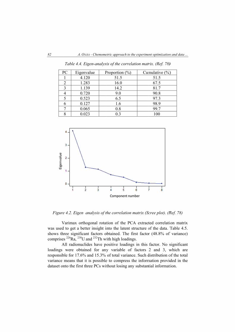
82

P

Figure

Vwas usedshows thrcomprise

Aloadings responsibvariance dataset on

A. ON

Table 4.4. E

PC Eigen1 4.12 1.23 1.14 0.75 0.56 0.17 0.08 0.0

e 4.2. Eigen

Varimax orthd to get a betree significas 226Ra, 238U

All radionuclwere obtai

ble for 17.6%means that into the first t

NJIA - Chemome

Eigen-analys

nvalue P120 283 139 720 523 127 065 023

analysis of t

hogonal rotattter insight iant factors oand 232Th w

lides have pned for any

% and 15.3% it is possiblethree PCs wi

etric approach

sis of the corr

Proportion (%51.5 16.0 14.2 9.0 6.5 1.6 0.8 0.3

the correlatio

ation of the into the latenobtained. The

with high loadositive loadiy variable of total vari

e to compresithout losing

to the experime

relation matr

%) Cum

on matrix (Sc

PCA extractnt structure oe first factordings. ings in this of factors ance. Such dss the informany substant

ent optimization

rix. (Ref. 78)

mulative (%)51.5 67.5 81.7 90.8 97.3 98.9 99.7 100

cree plot). (R

ted correlatiof the data. Tr (48.8% of

factor. No s2 and 3, w

distribution omation providtial informat

n and data ...

)

)

Ref. 78)

ion matrix Table 4.5.

f variance)

significant which are of the total ded in the tion.

DATA EVALU

Table 4

Var226

23

23

40

232

134

137

7BVari

% T

between Quantitatthe classiachieved Samples assigned

Figure

UATION

4.5. Varimax

riable 6Ra 8U 5U 0K 2Th 4Cs 7Cs Be iance Var

The PCA, apthe soil sam

tive estimatioification mafor 86.0% ofrom six locas they fell o

4.3. Score psamples acc

x rotated factsam

Factor 1 0.943 0.926 0.866 0.181 0.920 0.019 0.144 0.713

3.9068 48.8

pplied to themples accordon of the claatrix (Table of the samp

cations were on the border

lot of PC1 ancording to th

tor loadings mples. (Ref.

Factor 2-0.228-0.250-0.389-0.8660.091 -0.1460.565 0.216

1.410317.6

e given datding to theiassification e4.6). Overa

les. Most samisclassifie

rs between th

nd PC2 illusheir geograp

of radionucl78)

Factor-0.089-0.170-0.19-0.1250.124-0.884-0.582-0.0281.225

15.3

aset, has shir geographiefficiency coall, the correamples wered. Some samhe two classe

strating the daphical orig

lide activities

3 Comm9 00 01 05 04 04 02 08 01 6.5

8

hown a diffeical origin (ould be obtaect classificaaccurately

mples were ines.

differentiationgin. (Ref. 78)

83

s in soil

munality .950 .950 .937 .798 .871 .803 .678 .556 5422

81.8

erentiation (Fig. 4.3). ained from ation was classified.

incorrectly

n of soil )


Table 4.6. Classification matrix. (Ref. 78)

Class 1 2 3 4 5 6 7 8 9 10 11 12 13 14 15 Corr. class.

7 6 6 10 6 8 8 7 5 5 6 8 7 5 9

% 100 66.7 100 50.0 50.0 100 100 85.7 100 100 100 100 71.4 100 66.7 Finally, it was concluded that good classification (86% correct

classification of the dataset) between soil samples of different origin could be achieved by analyzing their gamma-ray spectra and applying principal component analysis.

In an interesting study dedicated to determination of elemental composition of atmospheric aerosol samples by using particle-induced X-ray emission (PIXE) spectrometry, PCA and factor analysis were employed79. Therefore, the PIXE data were reduced to few dimensions enabling a better look into the latent structure of the database.

This revealed three significant factors, which accounted for 83 % and 78 % of the total variance in the coarse and fine fractions, respectively. The loadings for the various factors in both size fractions were then converted into source profiles. According to the elements that are associated with the three factors (Table 4.7), it is evident that the three aerosol source types are mineral dust, biomass burning and sea salt.

Cluster analysis attempts to find sample groupings or clusters within data using criteria developed from the data itself. Since there is no measure of cluster validity that can serve as a reliable indicator of the quality of a proposed partitioning of the data, clusters are defined intuitively, depending on the context of the problem. Hence, deep understanding and knowledge about the problem is crucial prerequisite prior to clustering.

One should bear in mind that the threshold value for similarity is developed directly from the data. Hence, criteria for similarity are often subjective and depend to a large degree on the nature of the problem investigated, the goals of the study, the number of clusters in the data sought, and, of course, previous experience.

Table 4.7. Sources for the detected elements in aerosols. (Ref. 79)

Source type Coarse particles Fine particles Mineral dust Al, Si, Ca, Ti, Fe Al, Si, Ti, Mn, Fe

Biomass burning S, Cl, K, Zn, Ca S, K, Zn, Br Sea salt Na, Mg, Cl Na, Mg, Cl, Ca

DATA EVALUATION 85

Cluster analysis is based on the principle that distances between pairs of points (i.e., samples) in the measurement space are inversely related to their degree of similarity3.

There are several different types of clustering algorithms, such as K-means80, FCV81, and Patrick Jarvis82. However, the most interesting and the most popular algorithm is hierarchical clustering83.

Similarity matrix is in the focus of the hierarchical clustering experiment. For a start, there is a computing of the distances between all pairs of points in the data set. Each distance is then converted into a similarity value by using the following equation:

max

1 ikik

ds

d= − (4.2)

Here, sik is the measure of similarity between samples i and k, dik is Euclidean distance between them, and dmax is the distance between the two most dissimilar samples, which is also the largest distance in the data set.

Similarity values vary from 0 to 1. They are organized in the form of a table or square symmetric matrix. Then, the similarity matrix is scanned for the largest value, which corresponds to the most similar point pair. The two samples that make the pair are combined to form a new point located midway between the two original data points.

Removal of the rows and columns corresponding to the original two data points is carried out. The symmetry matrix is then updated to include information about the similarity between the new point and every other point in the data set. Scanning of the matrix is performed again and the new nearest-point pair is identified and combined to form a single point. The rows and columns of the two data points that were combined are removed, and the matrix is recomputed.

Linkage of all the points is attained with this procedure. As a result, a diagram called dendogram is obtained. It is a visual representation of the relationships between samples in the data set. One simple example is given in Figure 4.4. One of the main reasons for the popularity of this method lies in the fact that the interpretation of the results is intuitive.


Figure 4.4. Typical dendogram obtained in cluster analysis by using single linkage method

Some ways to compute the distances between data points and clusters in hierarchical clustering are shown in Figure 4.5. They include single, complete, and average linkage.

Figure 4.5. Computation for the distance between a data cluster and a point

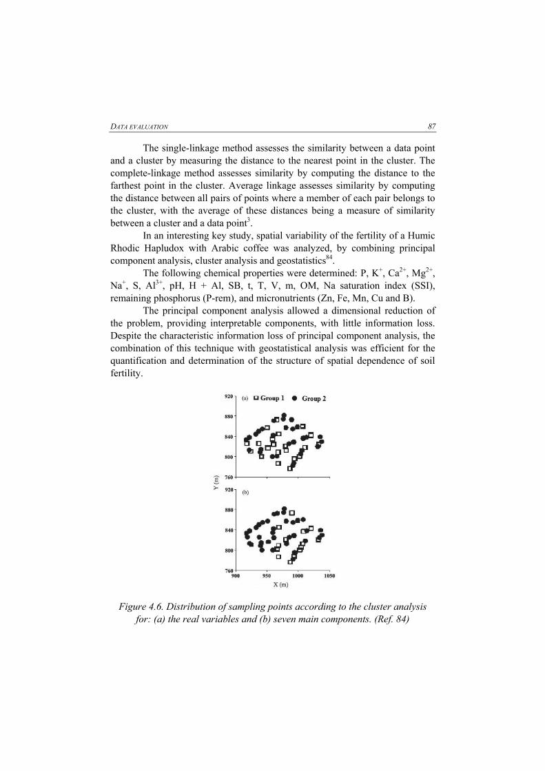
DATA EVALUATION 87

The single-linkage method assesses the similarity between a data point and a cluster by measuring the distance to the nearest point in the cluster. The complete-linkage method assesses similarity by computing the distance to the farthest point in the cluster. Average linkage assesses similarity by computing the distance between all pairs of points where a member of each pair belongs to the cluster, with the average of these distances being a measure of similarity between a cluster and a data point3.

In an interesting key study, spatial variability of the fertility of a Humic Rhodic Hapludox with Arabic coffee was analyzed, by combining principal component analysis, cluster analysis and geostatistics84.

The following chemical properties were determined: P, K+, Ca2+, Mg2+, Na+, S, Al3+, pH, H + Al, SB, t, T, V, m, OM, Na saturation index (SSI), remaining phosphorus (P-rem), and micronutrients (Zn, Fe, Mn, Cu and B).

The principal component analysis allowed a dimensional reduction of the problem, providing interpretable components, with little information loss. Despite the characteristic information loss of principal component analysis, the combination of this technique with geostatistical analysis was efficient for the quantification and determination of the structure of spatial dependence of soil fertility.

Figure 4.6. Distribution of sampling points according to the cluster analysis for: (a) the real variables and (b) seven main components. (Ref. 84)


Figure 4.6 shows a similarity of 70% between the actual set of properties and the seven principal components which together account for 79.81% of the variability, thus validating the use of an analysis that reduced the number of variables, facilitating interpretation.

In comparison, the cluster analysis across the seven principal components reduces the complexity of interpretation of soil properties of the analysis with 22 original data points. Here, as most of the variability is contained in the first and second components, the analysis is even simpler.

The reader is directed toward another useful application of the principal component analysis in analytical chemistry where concentrations of Cu, Zn, Mn, Fe, K, Ca, Mg, Al, Ba and B in 26 herbal drugs of special importance in phytopharmacy were studied85. Herein, four significant factors identified by principal component analysis were attributed partly to the significant influential sources and high mobility of some elements thus referring to potential anthropogenic contamination.

In another example, principal component analysis and cluster analysis were applied to classify the samples according to their microelement contents86,87. Microelements in soft winter wheat grain samples collected from all over Serbian wheat growing regions were analyzed quantitatively by atomic absorption spectrophotometry. Microelement contents differed markedly among wheat samples harvested from various regions. The most frequently occurring pattern is Fe > Mn > Zn > Cu > Pb > As > Cd > Hg. Four PCs, explaining 84% of total variance, correlate well with the following elements: PC1 with Cu, Mn, and Zn content; PC2 with Pb and As; PC3 with Cd; and PC4 with Hg. Iron fails to load significantly on any PCs. Physical meaning of PCs could be attributed to metabolic processes in wheat, soil type, vicinity of industrial centers and busy motorways, and application of agrochemicals.

There is another study dealing with the contribution of emissions to pollution by determining concentration of heavy metals (Cd, Co, Cr, Cu, Fe, Mn, Ni, Pb and Zn) in surface soils in the area surrounding the steel production facility in Serbia88. Analysis of variance revealed the influence of latitude, longitude and distance from the emission source on heavy metal concentrations in soil. Multivariate statistical techniques (cluster analysis and factor analysis) confirmed previous findings and were also used to investigate relationships between heavy metal concentrations and soil particle size fractions. Regression analysis showed that the latitude, longitude and distance from the source are good predictors of heavy metal concentrations in soil. Geostatistical analysis revealed the spatial distribution of heavy metal concentrations in soil and their correlation with prevailing winds in the investigated area.

DATA EVALUATION 89

The application of cluster analysis is also seen in work where the use of mosses as biomonitors of major, minor and trace element deposition around the largest thermal power plant in Serbia were presented89,90. Also, spatial variations were studied in the distribution of trace ionic impurities in the water-steam cycle in a thermal power plant based on a multivariate statistical approach91.

To conclude, it is obvious that exploratory data analysis techniques are often quite helpful in elucidating the complex nature of multivariate relationships. Therefore, cluster analysis is a common technique for statistical data analysis, used in machine learning, pattern recognition, image analysis, information retrieval, bioinformatics, data compression, and computer graphics, while PCA is mostly used for making predictive models.

4.1.2. Kohonen artificial neural network

The Kohonen type of an artificial neural network (ANN) is an iterative technique for solving the problem of representing data based on a single layer of neurons arranged in a box exhibiting a 2-dimensional plane of responses on its top (Figure 4.7). Each neuron is represented by a weight, which is a vector of the same dimension as the input signal.

Figure 4.7. Kohonen network - the neurons are represented as columns arranged in a quadratic matrix


Each neuron (a column) in this scheme is surrounded by 8, 16, 24, etc., neighbors in its first, second, third, etc., neighborhood rings. The topology of the Kohonen ANN can be considerably improved if the “toroid” boundary conditions are fulfilled. This means that the network at its right or top edge is “continued” at its left and low edge, respectively, and vice versa. Unfortunately, the toroid conditions decrease the available mapping-area for a factor of four compared to the same dimensional non-toroid ANN.

Namely, the maximal topological separation of two neurons in the Nnet x Nnet dimensional toroid ANN is Nnet/2 neuron positions long, while in the non-toroid ANN the maximal topological distance between two neurons is equal to Nnet positions. In cases when a large area for mapping is needed the possibility of a two times larger maximal topological distance between two neurons can be a predominant factor for the use of a non-toroid ANN. Larger maximal topological distances between neurons offer better possibilities for separation of clusters in the non-toroid ANN compared to the toroid ANN of the same size92.

The maximal topological distance between two neurons excited by two different objects does not necessarily mean that these two objects are the most separated ones in the measurement space of the treated objects. The frequency distribution of the objects is also affected by the topological distance of excited neurons in the Kohonen networks.

So, the input is passed to each neuron in the network. The neurons are competing among themselves which one will be stimulated and learning is usually referred to as a competitive learning. The selection of this neuron is crucial. The neuron whose weight vector is closest to the input signal is declared the winning neuron (the most excited or the central neuron) for which the weight vector is adjusted to more closely resemble the input signal.

Adjustment to a lesser degree is also done for the neurons which surround the winning neuron. Upon completion, similar input signals are caused to respond to neurons that are near each other in this process. The actual selection of the winning neuron (c) is based on the comparison between all weight vectors wj = (wj1, wj2, .... wjm) and the input signal Xs = (Xs1, Xs2, ......., Xsm) according to equation:

2

1

min ( )m

si jii

c x w=

← − (4.3)

where j=1, 2, 3, 4, .....Nnet x Nnet.

DATA EVALUATION 91

Initially, components of the vectors in the network are assigned random numbers (initialization). Next, the random weight vectors and the sample vectors in the data set are normalized to unit length. Presenting the data one pattern at a time to the network is used to perform the training. Between the pattern vector and each weight vector in the network is computed the Euclidean distance.

Due to use of the competitive learning, the sample is assigned to the neuron whose weight vector is closest. The weight vector of the winning neuron and its neighbors are then adjusted to more closely resemble the sample using the Kohonen learning rule3:

,( 1) ( ) ( )* ( )( )i i ic i i oldw t w t t d x wη α+ = + − (4.4)

where wi(t + 1) is the ith weight vector for the next iteration, wi(t) is the ith weight vector for the current iteration, η(t) is the learning rate function, α(dic) is the neighborhood function, and xi is the sample vector currently passed to the network. During a single iteration, the comparison of all sample data vectors to all weight vectors in the network and the modification of those weights is performed. The weights are renormalized to unit length after applying the learning rule.

The main requirement for learning is that the weights wci of the neuron c should be corrected next time. It should be done in such a way that the neuron c will be then even closer to Xs than before.

At any time, the point of the learning procedure, not only the excited neuron c, but also its 8, 16, 24. . . . . 8p neighbors in the first, second. . . . . p-th, neighborhoods are stimulated. However, to which p and to which extent the neurons are stimulated, depends on the parameters amax, amin, Nnet, and itot of the learning strategy:

( ) [ ]max min min( / ) ) * 1 / ( 1) ( )oldji net si jiw a a p N a d p x w Δ = − + − + − (4.5)

where d = 0, 1, 2, 3...., p. During the learning, the range p to which the neurons are still stimulated decreases as:

( ) / ( 1)tot it net totp i i N i= − − (4.6)

At the beginning of learning (iit = 1), p covers the entire network (p = Nnet) while at the end of the learning iteration steps (iit =itot ), p is limited only to the central neuron c (p = 0). The unsupervised training is usually carried out for a predefined number of training epochs or iteration cycles, itot.


After an itot number of training cycles (epochs) has been run through the ANN, the complete set of the training vectors Xs is once more run through the ANN. In its last run the labeling of the neurons excited by the input vectors is made into the table called top-map that has as many entries as there are neurons83.

If one neuron is excited by more than one object Xs which is called conflict, either the labels of all objects exciting this neuron are stored (if a program allows such storage) or only the most representative ones. Therefore, the top-map with labels has to be regarded only as partial information for a quick visualization.

As seen from Figure 4.7, the number of weights in each neuron is equal to the dimension m of the input vector Xs = (xs1, xs2, xs3,... xsm). Hence, each Kohonen network consists of (Nnet × Nnet) × m weights. Before learning starts, all weights in the ANN are randomized in the interval 0-1.

Each neuron has the same number of weights and always the same variable is passed to each weight at a fixed position in the neuron. Therefore, only data of one specific variable are handled in each level of weights. Consequently, at the end of learning in each level, a map showing the distribution of values of the particular variable is formed83.

It is vital to remember that at the end of learning each and every weight in the Kohonen artificial neural network is adapted to the data even if certain neurons and their weights were never excited by any object.

As can be seen from the top-map on Figure 4.8, objects that have participated in learning have been clustered into two groups: L and H. By inspection of all levels and the corresponding maps, it can be seen that the distribution of the values of the i-th variable (weight map of i-th weight level) corresponds quite well to the grouping of objects found in the top-map of the Kohonen artificial neural network.

DATA EVALUATION 93

Figure 4.8. Comparison of the i-th weight level with the top-map

It can be suggested that the rule for separation of unknown objects based on the values of the variable i is reasonable. On the other hand, it is difficult to come to solid conclusion by first inspection of weight maps obtained on a small number of objects83.

An advantage of self-organizing maps is that outliers affect only one map unit and its neighborhood, while the rest of the display is available for investigating the remaining data. For this reason, a single outlier has a small effect on the ending weights, because the neurons are more likely to represent areas of the largest sample density3.

In Kohonen ANN distance is not preserved in the mapping which is one of the biggest disadvantage of self-organizing maps. The massive number of computations often needed to reach a stable network configuration limits the size of the network, which is also a huge disadvantage. If too few neurons are used, clusters overlap in the map. In addition, information about class structure is lost. On the other hand, if too many neurons are used, then training becomes prohibitive. In such a network, most of the neurons would probably be unoccupied3.


Some of applicative features of Kohonen artificial neural network are discussed below. Following example shows how a selection of a small representative set is obtained from a large quantity of intensities in the spectral region from 4000 to 200 cm-1 in infrared spectroscopy. Namely, in a group of 3284 infrared spectra the spectra-structure correlation study is presented93,94.

Training and test sets are usually easily manually established when they contain a small number of data. However, if data sets contain more than 3000 full-curve infrared spectra as in this case, selection of data becomes a problem.

Only 512 (= 29) intensities in the range from 3500 to 550 cm-1 were selected although the original spectra contained more intensities. Fast Hadamard forward and backward transformation95 was used to achieve a 1:4 reduction of representation size (each spectrum was represented by 128 intensity points). The reduction is reflected mainly in a lower resolution.

The objective is to select approximately 20-25% of all spectra in the collection for the training set (about 800 out of 3284). Training set is used to generate the model which will be able to predict structural features of the molecules. For such a reason, in the training set compounds with many different fragments and, preferably, the occurrence of different fragments in the chosen set of structures is needed.

The inclusion of the most common fragments like benzene ring or carbonyl which are present in a large majority of data ensures the perfect balance of fragments. The goal is to select a group of compounds in which the heavily biased distribution of the most frequent fragments will be shifted towards less frequent ones. The rest of the data set up to 3284 spectra is for testing.

The procedure of selecting the representative set was started by training the 30 × 30 neurons large Kohonen artificial neural network with all infrared spectra. At the end of the relative short training of 20 epochs all 3284 infrared spectra were sent through the (30 × 30 × 128) Kohonen network again. For each neuron was counted how many and which spectra they have excited.

Since infrared spectra exciting the same neuron are always quite similar to each other, it was decided to select from each neuron only one spectrum (one compound) that has excited it. Because 145 neurons were not excited by any spectrum, a group of 755 spectra was selected to compose the training set. It is seen from table 4.8 that although 145 neurons were not excited at all, each of the remaining 755 neurons was excited by more than four spectra on the average. Nineteen neurons were excited by as many as fifteen and more spectra.

DATA EVALUATION 95

Table 4.8. Frequency distribution of multiple hits on the (30 × 30 x 128) Kohonen network

No. of neurons No. of hits No. of spectra 145 0 0 184 1 184 112 2 224 113 3 339 68 4 272 76 5 380 37 6 222 43 7 301 30 8 240 20 9 180 13 10 130 2 11 132 20 12 240 2 13 26 7 14 98 3 15 45 4 16 64 5 17 85 1 18 18 2 19 38 1 21 21 1 22 22 1 23 23

From all spectra {Xi}j that have excited neuron j the following

procedure was applied. The average spectrum Sj was calculated and next the spectrum from {Xi}y having the smallest distance to the average spectrum Sj was identified and selected for the representative set. This was repeated for all excited neurons in the network. 755 neurons were excited and then selected as the representative set.

One example of using Kohonen ANNs is the lead spatio-temporal pattern identification in urban microenvironments using moss bags96.


4.2. Supervised pattern recognition

In the supervised pattern recognition, objects belonging to two or more classes are selected for the measurements leading to the I x K matrix while in unsupervised situation, the objects are measured and the I x K matrix is constructed without prior knowledge of the existence of classes.

If clusters of object are found, by visual inspection or clustering techniques, methods of supervised clarification can be used on them. Many of the methods for clustering are based on the geometrical properties of the multivariate space. Especially Euclidean, or Minkowski and Mahalanobis distances can be used. Bayesian modeling, where the clusters are described by multivariate normal distributions is very useful, but also fuzzy clustering has to be mentioned97.

Supervised pattern recognition requires a training set of known groupings to be available in advance, since it tries to answer a precise question as to the class of an unknown sample. In many cases, chemical pattern recognition can be performed as a type of screening, with doubtful samples being subjected to more sophisticated tests3.

Supervised pattern recognition in this chapter cover discriminant analysis, k-nearest neighbor, soft independent modeling by class analogy (SIMCA), and feed forward artificial neural network.

4.2.1. Discriminant analysis

Discriminant analysis (DA) methods, such as linear discriminant analysis (LDA) or factorial discriminant analysis (FDA), are acknowledged chemometric approaches for solving classification problems in analytical chemistry. In most cases, principle components analysis (PCA) is used as the first step to generate orthogonal eigenvectors. The corresponding sample scores are used to generate discriminant features for the discrimination.

LDA is a pattern recognition method which is used in cases where class variance is asymmetrical98. It is widely used, especially in the field of food analysis, to obtain a comprehensive, multivariate description of the data without assigning particular signals to specific metabolites99.

LDA maximizes the ratio between both variances compared to the within-group variance. It searches for a linear function of the variable in multivariate space. When the number of variables is larger than the number of observations in multi-dimensional data, LDA cannot be used directly. Then, first principal component analysis is employed in order to compress the data

DATA EVALUATION 97

and to transform the original data set comprising of large number of inter-correlated variables into a reduced new set of variables.

LDA requires that the variance-covariance matrices of the predefined classes can be pooled. This is only possible when these matrices can be considered to be equivalent. This means that their 95% confidence ellipsoids have equal volume (variance) and orientation (covariance) in the space of the variables100.

It should be emphasized that LDA belongs to the so-called supervised pattern recognition methods. The main goal of these methods is to use learning (or training) objects to find a rule for allocating a new object of unknown group to the correct group.

For a start, LDA is used to find a linear discriminant function (LDF), which is designated as Y5. Practically, it is a linear combination of the original measured variables described by the equation:

1 1 2 2 ... n nY a X a X a X= + + + (4.7)

Now, a single value of Y comprises the original n measurements for each object. This way, the data have been reduced from n dimensions to one dimension. The coefficients of the terms are chosen in such a way that Y reflects the difference between the groups as much as possible. Objects in the same group will have similar values of Y and vice versa. Hence, discrimination between two groups is provided by LDF.

Let us consider the simplest situation where there are two classes and two variables, X1 and X2, like in Figure 4.9a. This diagram also shows the distribution of the individual variables for each group in the form of dot-plots. A considerable overlap in the distributions for the two groups is apparent for both the variables. LDF for these data is given as: Y = 0.91X1 + 0.42X2.

Line labeled Y in Fig. 4.9b represents this LDF. The value which the function takes for a given point is given by the projection of the point on to this line. Figure 4.9b shows the dot plots of the LDF, Y, for each group. There is no overlap between the distributions of Y for the two groups. Hence, Y is clearly better at discriminating between the groups than the original variables.


Figure 4.9. (a) Distributions of each variable between the two groups. (b) The distribution of the LDF for each group. (Ref. 5)

An unknown object will be classified according to its Y value. The approach is to compare Y with the mean Y values of the two groups. If Y is closer to Y1 than to Y2 then the object belongs to group 1, and vice versa. This method is satisfactory only if the two groups have similarly shaped distributions. In addition, if experience shows that a single object is more likely to belong to different group, then the decision rule will need to be modified.

There are several methods to test whether LDA has allocated an object correctly. For instance, classification rule can be used to classify each object in the group and to record whether the resulting classification is correct. The results of this procedure are listed in the table called the confusion matrix. This method tends to be overoptimistic since the object being classified was a part of the set which was used to form the rule.

Dividing the original data into two randomly chosen groups is a better way to test LDA. Here, the training set is used to find the LDF and subsequently, the objects in the test set are allocated using this function and the success rate found.

Another method that uses the data more economically is cross-validation (the “leave-one-out method“). It finds the LDF with one object omitted and checks whether this LDF then allocates the omitted object correctly. The procedure is then repeated for each object and again a success rate can be found.

DATA EVALUATION 99

Quadratic discriminant analysis (QDA) is used if the distributions do not have similar shapes . This modification of LDA assumes that the two groups have multivariate normal distributions but with different variancesError! Bookmark not defined..

In the following example, LDA was used to classify two types of fruit samples based on their rare earth element (REE) content. Namely, the açai (Euterpe oleracea Mart.) and jucara (Euterpe edulis Mart.) are plants naturally grown in Brazil which produce similar fruits rich in energy, minerals, vitamins and natural compounds with antioxidant and anti-inflammatory properties101. Although the drinks obtained from these species are similar, it is important to develop tools to establish the identity of the fruit species and growing regions.

To assess claims of origin and to investigate the differentiation of acai and jucara fruits based on REE content determined by ICP-MS, in particular Sm, Th, La, Pr, Gd, Ce and Nd, LDA was employed as a crucial aid. Principal component analysis was applied prior to LDA.

Two LDAs constructed with 28 samples of açai (n = 12) and jucara (n = 16) were tested. Two LDA models were obtained, one with all rare earth elements included (LDA-total) and the other one containing only the elements which showed homogeneity of variance and normal distribution for both species. The distance measure used in calculating sample separation was the Mahalanobis, and the larger the Mahalanobis distance between the two samples, the greater the differences between the REE levels.

The normal distribution of the samples was tested using the Kolmogorov-Smirnov test at 5%. The homogeneity of variance was tested using the Levene’s test at 1% level. It was noted that 6 REEs (Tb, Yb, Tm, Lu, Ho and Er) from acai fruit samples and 3 REEs (Th, Lu and Gd) from jucara samples had a non-normal distribution. The Levene’s test (p > 0.01) for homogeneity of variance has indicated that 4 elements (Sm, Tb, Th and Nd) have exhibited the heterogeneity of variance. After the distribution and homogeneity results were checked, two LDA models were run.

Model LDA-7 was formed using the REEs which showed normal distribution for both species and homogeneity of variance. The second model, LDA-total, was built with all the REEs included in Table 4.9. The LDA models were built with 12 samples of acai and 16 samples of jucara, and the accuracy of both models was 89.3%. However, the LDA classification accuracy was higher for LDA-7 (83.3%) than for LDA-total (66.7%) for the external classification.

Although 15 REEs were determined by ICP-MS, only 7 of them (Sm, La, Eu, Dy, Pr, Gd and Ce) had a normal distribution and homogeneity of


variance, the prerequisites for LDA analysis, and these have been included in the matrix LDA-7. The matrix LDA-7 was more accurate predictor than the LDA-Total matrix, which was composed of all analyzed REEs (Table 4.9).

Table 4.9. LDA classification and prediction of rare earth element concentration in acai and jucara fruit samples. (Ref. 101)

REE

LDA models (n=28) External classification (n=6) Incorrectly

classified samples Accuracy rate (%)

Incorrectly classified samples

Accuracy rate (%) Acai

(n=12) Jucara (n=16)

Acai (n=3) Jucara (n=3)

Sm, La, Eu, Dy, Pr, Gd, and Ce (LDA-7)

2 1 89.3 1 0 83.3

Sm, Tb, Th, La, Eu, Dy, Pr, Yb, Tm, Tu, Gd, and Nd (LDA-

total)

0 3 89.3 1 1 66.7

This demonstrates the importance of knowing the matrices being used

because normal distribution and homogeneity of variance form the basis for a solid model. LDA analysis differentiated correctly between species, with a predictive ability of 83.3% for an external validation fruit set using model LDA-7. On the other hand, if all REEs are used, the ability to differentiate acai and jucara fruits drops significantly, to 66.7% (Table 4).

The applied methodology confirms that REEs can be used to differentiate acai from jucara fruit samples and to guarantee the correct origin of products from the two species. LDA has been found as a useful tool in this factory.

4.2.2. K-nearest neighbor

Nearest neighbor methods are rather comprehensible way to classify an unknown object when there are two or more groups of objects of known class, since it does not require to elaborate statistical computations as is the case in the methods like SIMCA, discriminant analysis and dissimilarity based partial least squares (DPLS). The k-nearest neighbor (KNN) method has been extensively used in pattern recognition due to its conceptual simplicity, wide applicability, and efficiency.

The common use of the KNN method is based on an idea of using the Euclidean metric to measure distances between objects of the data set. In addition, the results of pattern recognition methods can be affected to a great extent by the use of different metrics. The problem arises since there is little

DATA EVALUATION 101

consensus as to which types of metrics or similarity coefficients are most generally applicable and in which cases.

Let us take a look at the figure 4.10 where two groups of objects are depicted. It is obvious that the groups cannot be simply separated by the plane. KNN could be used since it makes no assumptions about the distributions in the classes.

In its simplest form the method involves assigning the members of the training set to their known classes. The algorithm starts with a number of objects assigned to each class. The data should not contain outliers or samples with an ambiguous classification. In addition, the classes should be nearly equal in size in order to avoid bias when an unknown sample is assigned to a class.

Figure 4.10. Two groups which cannot be separated by a plane

The methodology of the k-nearest neighbor is implemented as follows53. As previously said, for a start, a training set should be assigned to known classes followed by calculation of the distance between an unknown to all members of the training set. This is conveyed by computing Euclidean distances but other distances could be used as well. The effectiveness of Euclidean distances is limited in many practical applications102,103,104. Distances should be ranked then. The smallest distance is ranked as 1, the next as 2, and so on.


Figure 4.11. Three nearest neighbors to unknown

If k = 1, only the closest neighbor and its class are taken into account and the unknown object is assigned to this class. In this case the shortest distance (d1) is associated to an object of the square class, and this means that the unknown object also belongs to this category.

The method considers the three closest objects in case that k = 3. Thus the unknown object is classified as belonging to the triangle class, because it receives two votes (d2 and d3) from the triangle class and only one vote (d1) from the square class.

In the specific case that there is a tie, the classification is based on the summed accumulated distances - the class with smallest accumulated distances is attributed to the object.

In figure 4.11 it could be seen that k = 3 and all objects belong to class B. It is useful to use more than one value of K. If different K-values result in changes in an object’s classification, it is then not very secure. So, the majority vote is used for classification. If K in some case was 5, one of the five closest objects would belongs to class A.

In more sophisticated versions of the method, voting schemes other than the simple majority is used. This may be appropriate if the different classes in the training set have notably different variances. In some applications each object is characterized by many variables, some of which may be strongly correlated, while others may have little value in the classification process5.

DATA EVALUATION 103

Final check could be performed at the end to spot anomalies or artefacts. It is inspected by changing the number of K values (3, 5, or 7) to see if the classification changes.

To address the limitation of applying Euclidean distances, many distance metric learning algorithms have been proposed for various pattern recognition tasks105,106,107.

First class of them adaptively select the neighborhood shape by learning a local metric. Although it performs effectively under non-linear decision boundaries in training samples, it needs some restrictive assumptions. Also, it suffers from high computational complexity.

Other algorithms are viewed as a global linear transform of the input space such as Mahalanobis metric108. However, since the number of training samples can be small, the estimation for distance metric is rather unreliable.

Although, KNN is a very simple approach which can easily be understood and programmed, it poses a number of limitations as follows: o the numbers in each class of the training set should be approximately

equal, otherwise the „votes“ will be biased towards the class with more representatives.

o for simple implementation, each variable is assumed to have an equal significance. Selecting the variables or using another distance measure solves the problem.

o ambiguous or outlying samples in the training set make problems in the resultant classification.

o the methods take no account of the spread of variance in a class. The last limitation is apparent in the example when forensic sample is

tested for forgery. It is likely that the class of forgeries has a much higher variance than the class of nonforged samples.

In the following example, the k-nearest neighbor method will be used to classify the representative elements into metals or nonmetals based on their periodic properties109. The properties that will be considered are atomic radius, first ionization energy, electron affinity and electronegativity. We will assume that the reader is already familiar with the regular periodical rules applied to metals, metalloids, nonmetals, etc.

For the beginning, the data matrix of 38 × 4 is constructed as given in Table 4.10. Here, there are 38 lines for chemical elements and 4 columns for periodic properties. Then, the geometric distance of an element from all other elements of the training set is calculated by using Eucledean distance. It is done using the following equation:


1/22 2 21 1 2 2( ) ( ) ... ( )n nd x y x y x y = − + − + + − (4.8)

where d is the distance between two points (chemical elements) in n dimensional space with coordinates (x1, x2, . . ., xn) and (y1, y2, . . ., yn). The distances are ranked in order and the class of an object is predicted according to the class of its k nearest neighbors. K assumes the values ranging from 1 to the maximum k value (kmax), which is the total number of objects in the training set decreased by one, but as the size of k approaches the number of objects in the training set, the comparisons are in fact made to far neighbors. Usually, several values of k are tried and the one with the best error rate is used in the end110.

Table 4.10. Elements and their four periodic properties selected to run the KNN method. (Ref. 109)

Element Atomic radius (pm)

Ionization energy

(kJ/mol)

Electron affinity (kJ/mol)

Electronegativity Group

Li 152 519 60 1.00 1 Na 154 494 53 0.93 1 K 227 414 48 0.82 1 Rb 248 418 47 0.82 1 Cs 265 402 46 0.79 1 Fr 270 376 44 0.70 1 Be 113 400 -66 1.60 2 Mg 160 900 -67 1.30 2 Ca 197 736 2 1.30 2 Sr 215 590 5 0.95 2 Ba 217 548 14 0.89 2 Ra 283 502 10 0.90 2 Al 143 509 43 1.60 13 Ga 122 577 29 1.60 13 In 163 556 29 1.80 13 Tl 170 590 19 2.00 13 Ge 122 784 116 2.00 14 Sn 141 707 116 2.00 14 Pb 175 716 35 2.30 14 Sb 141 834 103 2.10 15 Bi 155 703 91 2.00 15 Po 167 812 174 2.00 16

DATA EVALUATION 105

Nonmetal H 30 1310 73 2.20 - B 88 799 27 2.00 13 C 77 1090 122 2.60 14 Si 117 786 134 1.90 14 N 75 1400 -7 3.00 15 P 110 1011 72 2.20 15

As 121 947 78 2.20 15 O 66 1310 141 3.40 16 S 104 1000 200 2.60 16 Se 117 941 195 2.60 16 Te 137 870 190 2.10 16 F 58 1680 328 4.00 17 Cl 99 1255 349 3.20 17 Br 114 1140 325 3.00 17 I 133 1008 295 2.70 17

Al 140 1037 270 2.00 17

Classification technique such as KNN is quite similar to polling because every k closest object gives one vote for its class and then the object is assigned to the class with the most votes. Each object in the training set is compared to the others but not with itself which makes this technique self-validating.

Before running the KNN algorithm, the elements have been allocated their proper category (metal or nonmetal) in the matrix. The model built used auto scaled data and ten as kmax.

The results of KNN classification are shown in Table 4.11. In this table, C stands for correct and I for incorrect classification. The majority of the elements received a correct classification for all 10-nearest neighbors. Seven elements received a wrong classification: five nonmetals have been classified as metals, whereas two metals have been classified as nonmetals for at least one k value. Silicon was misclassified for all ten values of k, tellurium for nine; boron and germanium for four; polonium for three; arsenic for two; and phosphorus for only one. All these elements are metalloids, except phosphorus.


Table 4.11. Classification of the representative elements according to the KNN method. (Ref. 109)

Element K1 K2 K3 K4 K5 K6 K7 K8 K9 K10 Li c c c c c c c c c c Na c c c c c c c c c c K c c c c c c c c c c Rb c c c c c c c c c c Cs c c c c c c c c c c Fr c c c c c c c c c c Be c c c c c c c c c c Mg c c c c c c c c c c Ca c c c c c c c c c c Sr c c c c c c c c c c Ba c c c c c c c c c c Ra c c c c c c c c c c Al c c c c c c c c c c Ga c c c c c c c c c c In c c c c c c c c c c Tl c c c c c c c c c c Ge i i c c c c i c i c Sn c c c c c c c c c c Pb c c c c c c c c c c Sb c c c c c c c c c c Bi c c c c c c c c c c Po i i c c c c c c i c

Nonmetal H c c c c c c c c c c B c c c c c c i i i i C c c c c c c c c c c Si i i i i i i i i i i N c c c c c c c c c c P c c i c c c c c c c

As c c i c c c i c c c O c c c c c c c c c c S c c c c c c c c c c Se c c c c c c c c c c Te i i i i i i i i i i F c c c c c c c c c c Cl c c c c c c c c c c Br c c c c c c c c c c I c c c c c c c c c c

Al c c c c c c c c c c As a conclusion, the separation between metal, metalloid, and nonmetal

elements as traditionally drawn by a simple line in the periodic table is

DATA EVALUATION 107

dependent on the property under consideration. Normally, periodic properties that make the distinction are not as rigid as KNN classification assumes. Actually, a perfect classification would only be possible if each element in both classes has a distinct range of these properties, that is, there should be no overlap in multidimensional space, which is not the case with KNN.

KNN methods have been applied to many problems in analytical chemistry and related areas. For instance, they are used in classifications based on chromatographic or spectroscopic data of various samples including foodstuffs, soil, water and other environmental samples.

4.2.3. Soft independent modeling of class analogy

Soft independent modeling of class analogy (SIMCA) is a supervised classification technique that uses principal component analysis or partial least squares regression for classification by creating confidence region around each class using residuals of the samples in the calibration set53.

SIMCA was introduced by Svante Wold in the early 1970s as a pattern recognition technique in which new objects are projected as a member of a particular class based on their Euclidian distance from its particular principle component space. Euclidian distance does not exceed a confidence limit from a particular principle component. The number of principal components which is retained for each class is usually determined directly from the data by using a so called cross validation which is often different for each class model3.

When two classes can overlap this makes them soft and it is normal that an object belongs to both or neither class simultaneously. In hard modelling object must belong to a discrete class (for instance, when analyst wants to prove the presence of a drug in the blood serum by using appropriate method, there are only two options: either the test is positive or not). The problem with soft modeling is rather common especially in chemistry since a single compound may possess both carboxylic and amino group and thus belong to acids and amines at the same time. Therefore, it is entirely legitimate for an object to fit into more than one class simultaneously.

The samples in the overlapping region represent intermediates between the two overlapping classes and they partly belong to both of them (Figure 4.12). Classification in SIMCA is made by comparing the residual variance of a sample with the average residual variance of those samples that make up the class. This comparison provides a direct measure of the similarity of a sample to a particular class and can be considered as a measure of the goodness of fit of a sample for a particular class model.


Figure 4.12. Example of two overlapping classes of data

Concretely, SIMCA is used to determine whether the sample belongs to one class or another, if samples are available for the reference class. For such a matter, some a priori knowledge about the object and classes is required. In case it is not sufficient, a preliminary reference set can be obtained by ordination of the samples, using principal component analysis, multi-dimensional scaling or cluster analysis (dendrogram). The composition of this initial reference set needs to be refined in order to get a good final model. The number and identity of the samples to be included are the most important issues in selection of a reference set. Wrong selection of samples in the reference set would destroy the model.

Figure 4.13. A set of reference samples plotted together with some non-reference samples

DATA EVALUATION 109

It is rare that samples give a model with high homogeneity, which limits the model’s validity and usage. In contrast, many samples may give a model that spans the whole variation range, but samples do not belong to the true reference set are included. This causes false classification of the test samples. The challenge is thus to find the balance between maximal homogeneity and maximal variation span111.

SIMCA can also be treated as a multivariate outlier test because it checks outliers in the space of the selected principal components. The variation in the data not explained by the principal component model is called the residual variance. On the basis of residual variance of the objects in the training set, residual standard deviation (s0) is calculated as:

2

1 10 ( 1 )( 1)

m n

ikk ie

sm a m a

= ==− − − −

(4.9)

where e2ik is the residual of object, k is the calibration set for variable i,

m is the number of observations in the calibration set, n is the number of variables and a is the number of principal components. The residuals of the training set follow normal distribution. From this reason, the F-test may be used to describe the critical value of Euclidean distances of the objects towards the model. This test could be represented by the equation as:

20sFs critcrit = (4.10)

where Fcrit is the tabulated value for the specific degree of freedom at a significant level. For a new object x j

new that belongs to a certain class having residual vector eji

new, the residual standard deviation (sj) is calculated as:

2

1( )

( 1 )

n newjii

j

es

m a==− −

(4.11)

In order to estimate weather the residual variance sj is significantly different from the pooled residual variance s0 of the model, Fj

new should be calculated and compared with its tabulated critical value Fcrit by using the following equation:

2 20/new

j jF s s= (4.12)


Mahalanobis distance (MD) proposed by Hawkins is used instead of Euclidean distance for multivariate outlier tests53. Generally, the samples that may be described by spectra are mapped onto a much lower dimensional subspace for arrangement and if a sample is comparable to the other samples in the class, it will lie closer to them in the principal component map defined by the samples indicating that class.

SIMCA has several advantages in classification of data. Firstly, an unknown sample is only assigned to the class for which it has a high probability. If the sample’s residual variance exceeds the upper limit for every class in the training set, the sample would not be assigned to any of these classes because it is either an outlier or is from a class not represented in the training set.

Another advantage of SIMCA occurs when some of the classes in the data set cannot be well separated. In this case, sample might be assigned to two or more groups by SIMCA.

Also, SIMCA is sensitive to the quality of the data used to generate the principal component models for each class in the training set. There are diagnostics to assess the quality of the data as a result of using principal component analysis. For this purpose modeling power is used in order to describe how well a variable helps each principal component to model variation in the data, while discriminatory power describes how well a variable helps each principal component model to classify samples. Since variables with low modeling power and low discriminatory power contribute only noise to the principal component models they usually can be deleted from the analysis.

In the following example, the SIMCA method has been applied to the interpretation of the polycyclic aromatic hydrocarbons (PAHs) content in soil in different sites and from different times112. The soil samples were collected at six locations near the oil refinery in Novi Sad (Serbia). Gas chromatography was employed to detect eleven PAHs: (phenanthrene, anthracene, fluoranthene, pyrene, benzo(a)anthracene, chrysene, benzo(b+k)fluoranthene, benzo(a)pyrene, dibenzo(a,h)anthracene, benzo(g,h,i) perylene, and indeno(1,2,3,c,d)pyrene). The SIMCA data analysis was carried out by means of PLS Toolbox 2.1 software package.

DATA EVALU

Trange betPAHs (vamodelingforming atermed a two directreated intraditionasplit into classes sim

Eanalysis iprincipal are the firfall mainlThe varia

Uwith all approximremaining

UATION

The measuredtween 0.75 aariables) in

g. Each soil sa data vecto„class“. In tctions (Figurndependentlyal principal c

two classesmultaneously

Each class win the way thcomponentsrst two princly into a boxance explaineUsing the asssamples in

mately a halfg samples in

Figure

d data indicaand 86.2 μg/g94 soil sampsample was cor while vecthe principal re 4.14) whiy. Therefore,component ans. Additionaly, hence therwas indepenhat each class. Class 1 falcipal componx, which is deed by these psigned classiboth the traf randomly the testing s

e 4.14. Score

ate that the cg dry soil. T

mples (observconsidered a

ctors belongi component ich indicates, SIMCA monalysis. Acclly, some sare is an overlndently modss could be dlls roughly wnents of this efined by theprincipal comification, theaining and tchosen sam

set (predictio

e plot of soil

concentrationThe concentravations) was as an assembing to the sspace, the sas that the dodeling shoucording to figmples belonlap region. deled using described by within the pla

class, whilee first three c

mponents is ge model wastesting set (r

mples in the on).

samples. (Re

ns of PAHs ation matrix used for mu

bly of elevename group wamples are scata are suitauld be used gure 4.14, th

ng to both (o

principal ca different n

ane, the axese the membercomponents ogiven in tables built and trecognition);

training se

ef. 112)

111

are in the x of eleven multivariate n variables were then cattered in able to be instead of

he data are or neither)

component number of s of which rs of class of class 2. e 4.12. tested: (a) ; (b) with

et and the


Table 4.12. Classification results using SIMCA. (Ref. 112)

No. PCs

Variance%

Error %

Recognition Class1 2 90.5 0.00 Class2 3 89.6 4.26 Prediction Class1 2 86.8 6.82

Class2 3 92.6 2.27 In all cases, the leave-one-out method of cross-validation was applied.

In the SIMCA model, 100 and 95.7 % of the soil samples were correctly classified, and 93.18 and 97.7 % of the soil samples were correctly predicted. Thus, good recognition and prediction success rates of the soil samples were obtained.

4.2.4. Feed forward artificial neural network

A feed forward artificial neural network (ANN) is an artificial neural network wherein connections between the units do not form a cycle as usually. Here, the information moves in only one direction, forward, from the input nodes, through the hidden nodes and to the output nodes but there are no cycles or loops in the network.

A general type of feed forward ANNs consists of three types of layers. They include layer of inputs, a layer of output neurons, and one or more hidden layers of neurons. This type of a three-layer feed-forward ANN is depicted in Figure 4.15.

Figure 4.15. A general type of three layered feed-forward ANNs

DATA EVALUATION 113

The sum of the products of the weights and the inputs is calculated in each node. If the value is above some threshold (typically 0) the neuron fires and takes the activated value (typically 1). In other case, it takes the deactivated value (typically -1). Neurons with this kind of activation function are also called artificial neurons. The term perceptron often refers to networks consisting of just one of these units.

A perceptron can be created using any values for the activated and deactivated states as long as the threshold value lies between the two. Most perceptrons have outputs of 1 or -1 with a threshold of 0 and there is some evidence that such networks can be trained more quickly than networks created from nodes with different activation and deactivation values.

Typically, feed forward ANNs are used for parameter prediction and data approximation. One of the main types of this network is a cascade type of feed-forward ANNs, which consists of a layer of input, a layer of output neurons, and one or more hidden layers. Similar to a general type of feed forward ANNs, the first layer has weights coming from the input but each subsequent layer has weights coming from the input and all previous layers while all layers have biases. The last layer is the network output. The initialization of each layer’s weights and biases is performed at the beginning113.

The training process determined through a back propagation algorithm minimizes a quadratic error between the desired and network outputs. For training considered artificial neural networks the gradient descent method with momentum weight/bias learning rule is used. This is a developed algorithm of the basic back propagation algorithm.

A net input (Vj) to a neuron in a hidden layer k is calculated by using the following equation:

1

n

j ji i ji

V W=

= Θ + Θ (4.13)

Here n is the number of k-1 layer neurons for a general type of feed forward neural network and the number of all of the previous layer neurons for a cascade type of feed forward networks. Weights are designated as Wji and the threshold offset as qj.

Activation function is determined by the output of the neuron Oj. It has effects on neuron outputs, which undermine compression of propagated signals and simulation of the nonlinearity of the complex systems.


In feed-forward neural networks several activation functions are used such as linear (Eq. 4.14), log-sigmoid (Eq. 4.15), and Tan-sigmoid (Eq. 4.16) as given:

( )j j jO Pureline V V= = (4.14)

( ) ( )( )1 / 1 jVj jO Logsig V e

−= = + (4.15)

( ) ( )( ) ( )( )2 21 / 1j jV V

j jO Tansig V e e− −= = − + (4.16)

Weights and biases are only updated after all the inputs and targets are presented to the artificial neural network. Subsequently, the average of system error should be minimized to increase learning performance by using the equation as given:

2

1 1

1( ( ) ( ))

2

N M

AV j ji j

E d n o nN = =

= − (4.17)

In this equation dj (n) is the desired output oj (n) is the network output, and N and M are the total number of training data sets and the number of neurons of the output layer.

In the gradient descent method, improved values of the weights can be achieved by making incremental changes Δwji proportional to əEAV/əWji according to equation:

AVji

ji

EW

Wη ∂

Δ = −∂

(4.18)

where the proportionally factor η is called the learning rate. Large values of η in the gradient descent formulation may lead to large oscillation or divergence.

One attempt to increase the speed of convergence while minimizing the possibility of oscillation, or divergence, involves adding a momentum term to the basic gradient descent formulation. In this case the weight vector at time index (k+1) is related to the weight vectors at time indexes (k) and (k-1) by the following formula:

( 1) ( ) ( 1)E

W k W k W kW

η β∂ + = − + Δ − ∂ (4.19)

DATA EVALUATION 115

The new weights for the step (k+1) are given as:

( 1) ( )ji j j jiW k o W kηδ β+ = + Δ (4.20)

where a momentum coefficient, or an acceleration parameter β is used to improve convergence.

The expression of δj is given by the following equations:

0.5( ) '( )k k k kd o f vδ = − (4.21)

'( )j k k kjk

f v Wδ δ= (4.22)

Equation 4.21 is used for output and Equation 4.22 for hidden neurons. The determination of minimum number of necessary hidden neurons and hidden layers is completely practical113.

In the following example, application of feed forward artificial neural network in recognition and classification of soils samples of an unknown geographic origin is presented114. Various soil samples were collected at different locations in Serbia and Montenegro and differentiated into classes. Radionuclide (226Ra, 238U, 235U, 40K, 134Cs, 137Cs, 232Th, and 7Be) activities from soil samples detected by gamma-ray spectrometry were used as inputs to ANN.

Five different training algorithms with different numbers of samples in training sets were tested and compared in order to find the one with the minimum root mean square error (RMSE). The best predictive power for the classification of soils from the fifteen regions was achieved using a network with 7 hidden layer nodes and 2500 training epochs using the online back-propagation randomized training algorithm.

In this key study, by using the optimized artificial neural network, most soil samples not included in the network training data set were correctly classified at an average rate of 92%.

The architecture of the neural network models employed herein is a fully connected feed forward system. As in ordinary case, signals propagate from the input layer through the hidden layer to the output layer. This way, a node receives signals via connections or weights from other nodes (or from the external world for the nodes of the input layer). The net input for a node j is given by the following equation:

j ji ii

net w o= (4.23)


Here i stands for the nodes in the previous layer, wji is the weight associated with the connection from node i to node j, and oi is the output of node i. The output of a node is determined by a nonlinear transfer function and the net input of the node.

The transfer (activation) function is used as a sigmoidal function:

{ }( ) 1/ 1 exp (j j j jo f net net = = + − + Θ (4.24)

Here, θ is a bias term or threshold value of the node j responsible for accommodating nonzero offsets in the data115.

In the testing phase, the trained ANN is fed by a separate set of data. The neural network predictions (using the trained weights) are compared with the target output values.

The neural network will produce almost instantaneous results for practical inputs provided. When the training and testing phases are found successful, the ANN is used for practical problems.

The success of the training process was estimated by the root mean square error (RMSE) which is calculated as:

1/2

1

( ) / /n

i ii

RMSE d o n x=

= − (4.25)

Here, di stands for the desired output (experimental values) in the training or testing set, oi stands for the actual output (predicted values) in the training or testing set, n is the number of data in the training or testing set, and x is the average value of the desired output in the training or testing set.

In this study, five different training algorithms were tested and compared. These algorithms include online back-propagation (OBP), online back-propagation randomized (OBPR), batch backpropagation (BBP), resilient propagation (RP), and quick propagation (QP).

The idea of the backpropagation algorithms is to propagate the error back through the network and to adjust the weights of each layer as it propagates.

OBP updates the weights after each pattern is presented to the network. In the OBPR algorithm, the order of input patterns is randomized prior to each epoch, which makes the learning process stochastic.

In the BBP algorithm, weight updates occur after each epoch. RP is an adaptive learning rate method where weight updates are based only on the sign of the local gradients, not on their magnitude.

DATA EVALUATION 117

Each weight has its own updated value, which varies with time. QP is a training method with a fixed learning rate that needs to be chosen to suit the problem.

Activities (Bq/kg) of radionuclides in the analyzed soil samples were determined and given in Table 4.13.

The classifier used was a three-layer network architectured by an input layer consisting of the radionuclide activities in the soil samples, a hidden layer, and an output layer composed of the regions the samples were collected from.

The strategy used for the classification of soils was the so-called one of many encoding116. The output of the network was a multi-dimensional vector, and each vectorial dimension class was assigned to a class.

Table 4.13. Descriptive statistics of radionuclide activities (Bq/kg) in soil samples. (Ref. 114)

Variable Mean SD Min Max Median Skewness Kurtois 226Ra 30.8 9.14 13.6 54.9 29.9 0.42 -0.45 238U 29.7 9.42 14.6 53.4 30.2 0.44 -0.33 235U 1.37 0.46 0.51 2.61 1.38 0.53 0.22 40K 567 164 271 919 593 -0.17 -0.73

232Th 40.7 13.5 18.3 83.4 39.7 1.20 2.18 134Cs 0.09 0.07 0.02 0.26 0.05 0.91 -0.56 137Cs 48.3 26.2 5.25 112 42.9 0.44 -0.39 7Be 1.79 1.05 0.54 3.94 1.50 0.66 -0.91

In the network training file, the class membership of a single data item

was coded in a numerical format, assigning 1 to the class where item belonged, and 0 to all the others. In the network testing file, the membership of an input data set was assigned to the class with the greatest network output.

As the division method for the selection of objects (training set) used for building the model, random selection within each region was applied. There are two advantages of this method: it is rather simple; and a group of data randomly taken from a larger set retains the population distribution of the entire set117.

The 103 objects were divided into training and test sets in seven different ways: 85 vs. 18, 75 vs. 28, 65 vs. 38, 55 vs. 48, 45 vs. 58, 35 vs. 68, and 25 vs. 78. The “leave-10%-out” method was applied for cross-validation. With this method, 10% of the data in the training set are not used to update the weights. Therefore, this 10% can be used as an indicator of whether or not memorization is taking place. When an ANN memorizes the training data, it


may produce acceptable results for the training data, but poor results when tested on unseen data.

In table 4.14, the RMSE for the prediction on the test set, applying five training algorithms to different training sets are given. It is obvious that the OBPR training algorithm gave the lowest RMSE. As opposite, an increase in RMSE with a decrease in the number of objects in the training set is manifested.

Table 4.14. RMSE of test set predictions as a function of the training algorithm and the number of objects in training/testing set (N). (Ref. 114)

N RMSE OBP OBPR BBP RP QP

85/18 0.116 0.108 0.123 0.159 0.135 75/28 0.092 0.087 0.096 0.125 0.102 65/38 0.102 0.102 0.106 0.138 0.118 55/48 0.119 0.115 0.118 0.143 0.137 45/58 0.125 0.121 0.126 0.152 0.147 35/68 0.143 0.135 0.141 0.172 0.159 25/78 0.144 0.141 0.152 0.181 0.186

This is understandable since the modeling area is more evenly covered

when more data are used in the training set. On the other hand, the best model was not obtained with the largest training set (85 vs. 18) but with the next largest division, i.e., 75 vs. 28. When too many training data are presented to the network, it tends to learn the specific data set better than the general problem.

The differences in RMSE values within a training/testing set of a fixed size cannot distinguish between the specific training algorithms in a significant manner. The greatest difference reached a factor of 1.5 (case 85/18; the best RMSE = 0.1080, the worst RMSE = 0.1586), while the most homogenous RMSE values were obtained with the training set of 55 objects, where the best and worst RMSE did not differ by more than 19%. This means that a thorough investigation for the proper selection of the training set size should be made as well as for the most suitable training algorithm.

The ANN model using the OBPR algorithm, which gave the lowest RMSE, was further optimized with 75 objects in the training set. Different combinations of the learning rate and momentum were used to find the best configuration for model optimization in order to allow the solution to escape the local minima of the error function. For this study, the learning rate and momentum were set at 0.1. The number of epochs and number of nodes in the

DATA EVALUATION 119

hidden layer were also optimized. Each topology was repeated five times to avoid random initialization of weights. The obtained results are presented in figure 4.16. Through the above process, it was found that the optimum number of hidden layer nodes was seven, and the number of learning epochs 2500.

Figure 4.16. The influence of number of epochs (ne) and number of hidden layer nodes (nl) on RMSE. (Ref. 114)

The ANN optimized in this study is schematically represented in Figure 4.17. The input layer consists of eight nodes representing the radionuclide activities. The output layer consists of fifteen nodes representing the regions the samples were collected from. In addition, there is also a bias (neuron activation threshold) connected to the nodes in the hidden and output layers (but not in the input layer) via modifiable weighted connections.


Figure 4.17. Schematic representation of a three-layer feed forward neural network. (Ref. 114)

A dataset not used in the training process was employed after the learning process to test the reliability of the trained algorithm. By using different sets of randomly chosen objects, the process was repeated 10 times. The overall performance of the predictive classifier based on neural network can be appreciated in detail by the classification matrix. In this matrix, the classes predicted by the ANN classifier are compared to the actual classes.

An ideal classifier will produce a classification matrix in which all diagonal elements are 100%, while all off-diagonal elements are 0%. The average classification rate defined as the ratio of the number of correctly identified patterns to that of all test patterns (the average of diagonal elements in the classification matrix) was 92.1 ± 5.23%.

It was shown that the performance of artificial neural networks outperformed principal component analysis (PCA) for the same data set. This method produced 86.4% of correctly classified soil samples. The feed forward artificial neural network method has shown many advantages over traditional methods for the analysis of gamma-ray spectra. Compared with the usual automatic spectrum analysis methods, this method use full-parallel computing and it is simple to implement.

In another example, feed forward artificial neural network (ANN) model was used to link molecular structures (boiling points, connectivity indices and molecular weights) and retention indices of polycyclic aromatic

DATA EVALUATION 121

hydrocarbons (PAHs) in linear temperature- programmed gas chromatography118. A randomly taken subset of PAH retention data reported by other authors, containing retention index data for 30 PAHs, was used to make the ANN model. The prediction ability of the trained ANN was tested on unseen data for 18 PAHs from the same article, as well as on the retention data for 7 PAHs experimentally obtained in this work. In addition, two different data sets with known retention indices taken from the literature were analyzed by the same ANN model. It has been shown that the relative accuracy as the degree of agreement between the measured and the predicted retention indices in all testing sets, for most of the studied PAHs, were within the experimental error margins (+-3 %).

Illustrative example is work by Dragović et al where a three-layer feed-forward neural network was developed to classify mosses and lichens according to geographical origin119. The activities of radionuclides (226Ra, 238U, 235U, 40K, 232Th, 134Cs, 137Cs and 7Be) detected in plant samples by gamma-ray spectrometry were used as inputs for neural network. Five different training algorithms with different number of samples in training sets were tested and compared, in order to find the one with the minimum root mean square error. The best predictive power for the classification of plants from 12 regions was achieved using a network with 5 hidden layer nodes and 3,000 training epochs, using the online back-propagation randomized training algorithm.

Implementation of this model to experimental data resulted in satisfactory classification of moss and lichen samples in terms of their geographical origin. The average classification rate obtained in this study was (90.7 ± 4.8)%.

Another example is an ANN modeling approach in a chemical speciation of metals in unpolluted soils of different types with the focus on the metals correlation with soil characteristics120.

These approaches are useful when a fast response combined with reasonable accuracy is required. The resistance to noise is certainly one of the most powerful characteristics of this type of analysis. In hazardous environments, automated pattern-recognition systems (such as neural networks) have a distinct advantage over traditional sampling and laboratory analysis methods since the environment can be monitored without risk to human operators.

4.2.5. Multiway pattern recognition (Tucker, Parafac, Unfolding)

Multiway data have raised significant interest in practical fields of chemometrics in recent time. It undermines a set of data for which the elements


depend on three or more directions. In three-way methods, multi-way data are characterized by several sets of variables that are measured in a crossed fashion, so instead of organizing the information as a two-dimensional array, it falls into a three-dimensional box.

Let us discuss the differences between one-, two-, and three-way data. One-way data consists of either one sample and multiple variables, for instance, a single chromatogram generated over time, or multiple samples and one variable, such as calibration of an ion-selective electrode. A single gas chromatogram collected with a flame-ionization detector is considered one-way data, as the data is only collected in one way, over time. Analyzing multiple solutions with an ion selective electrode is also one-way, over samples. In these applications, the mathematical and statistical tools applicable to one-way data analysis limit the analyst3.

As ordinary, the most of practice is devoted to two-way data analysis represented by matrices. Two-way data consists of multiple samples, each represented by multiple variables, or one sample represented by two sets of interacting variables. The type of two-way data determines the amount of quantitative and qualitative information that can be extracted121. Digitized ultraviolet spectra collected for each of I samples is an example of multiple samples (the first way) and multiple variables (the second way) forming two-way data. Such data is usually employed for quantitative applications where the independent variables, the spectra, are related to a concentration of the samples, which is the dependent variable3. Graphical presentation of nature of two- and three-way data is given in figure 4.18.

Figure 4.18. Difference between (a) Two-way and (b) three-way data

Three-way data is in chemical applications visualized as multiple samples, each consisting of two sets of interacting variables. It can also be formed with two object ways and one variable way and by one sample with three variable ways. Environmental data where several distinct locations are monitored at discrete time intervals for multiple analytes, exemplifies three-way

DATA EVALUATION 123

data with two object ways and one variable way. The data with three directions can be geometrically arranged as shown in Figure 4.19.

Figure 4.19. Representation of a three-way array applied in chromatography

Here, for two-way matrices the terms rows and columns are used. Vectors in the third mode will be called tubes. A slab, layer or slice of the array denotes a sub-matrix of the three-way array with two dimensions. In above case, a slab refers to a single sample so that one can define slabs in the other directions if necessary.

Applications of a three-dimensional data array are found in many modern analytical techniques. For instance, in hyphenated chromatography the detector records a signal, usually a current intensity, as a function of both an elution and a spectral dimension122,123.

In excitation-emission fluorescence, the intensity of the light emitted by a sample is recorded as a function of both the excitation and the emission wavelengths124. As opposite, in sensory analysis a two-dimensional data table of results is obtained when different assessors for several attributes judge a product125.

In all these cases, when more than one sample is measured, a so-called three-way array of data (data cube) is obtained, as each signal is now a function of three different sources of variation (in the case of chromatography: the sample, the elution time and the wavelength, or m/z ratio), and higher-order arrays can be obtained when more complicated experimental setups, such as GC–GC–MS are used.


The main advantage of three-way calibration is estimation of analyte concentrations in the presence of unknown, uncalibrated spectral interferents. These methods also permit the extraction of analyte, and often interferent, spectral profiles from complex and uncharacterized mixtures.

There is no limit to the number of ways that can form a data set, so there may be n-way data. For instance, four-way data is found in a collection of excitation-emission-time decay fluorescence spectra. If, for instance, varying experimental conditions is involved, five-, six-way data etc. is formed.

Multiway arrays represent a particularly rich source of information, as they often contain a large degree of redundancy, because many signals are used to describe a single sample. Motivated by this problem, specific mathematical and statistical tools have been developed to take the maximum advantage from the analysis of these kinds of data. We will consider Tucker3, PARAFAC, and unfolding models.

Tucker models are used for decomposition of single-block multiway data arrays. These models were introduced by Ledyard Tucker in the early 1960s126,127. The most important feature of Tucker models is that they allow the possibility of interaction between the factors.

Tucker3 models involve calculating weight matrices corresponding to each of the three dimensions (e.g. sampling site, date and metal), together with a core box or array which provides a measure of magnitude53. The three weight matrices do not necessarily have the same dimensions, so the number of significant components for the sampling sites may be different to those for the dates, unlike normal principal component analysis where one of the dimensions of both the scores and loadings matrices must be identical. This model (or decomposition) is given in figure 4.20.

Figure 4.20. Presentation of Tucker3 model

Tucker3 model is mathematically expressed as a weighted sum of outer products from all possible triads (or polyads for more than three modes) of

DATA EVALUATION 125

components, stored as columns of the loading matrices A(IxD), B(JxE) and C(KxF). As a different number of factors can be extracted for each mode:

D E F≠ ≠ (4.26)

The relative contribution of each outer product term to the description of the array X is expressed by means of a so-called core array G. This is a (DxExF) array whose def-th element indicates the magnitude of the interaction among the d-th column of A, eth column of B and f-th column of C. Mathematically it can be expressed as:

( ) ( ) ( )( )IxJK DxEF T IxJKX AG C B E= ⊗ + (4.27)

where G(DxEF) corresponds to the core array G unfolded to a DxEF matrix. This is given in algebraic form as:

1 1 1

D E F

ijk id je kf defd e f

x a b c g= = =

≈ (4.28)

where aid, bje and ckf are the id-th element of A, je-th element of B, and kf-th element of C, respectively, while gdef is the def-th element of G.

Apart from Tucker3, there are also two Tucker models more: Tucker2 and Tucker 1. We concluded that Tucker3 models assume that, in decomposing the three-way array X, all the three modes are reduced. This goes like this: D<I, E<J and F<K. However, there can be cases where only two of the three modes are compressed, while one is not reduced. This is the basics of the models called Tucker2. If only one of the modes is compressed to a reduced number of factors, the corresponding model is called a Tucker1 model128.

Though there is a clear gain in the quality and quantity of information when going from two- to three-way data sets, the mathematical complexity associated with the treatment of three-way data sets can seem, at first sight, a drawback. To avoid this problem, most of the three-way data analysis methods transform the original cube of data into a stack of matrices, where simpler mathematical methods can be applied. This process is often known as unfolding (Figure 4.21).


Figure 4.21. Three-way data array (cube) unfolding or matricization

Parallel factor analysis (PARAFAC) is a decomposition method for three-way arrays that can be seen as a simplification of bilinear principal component analysis to higher order arrays. In this model each of the three dimensions contains the same number of components which is the main difference from Tucker3 model. Each component consists of one score vector and two loading vectors instead of one score and one loading as in principal component analysis.

This model originated from psychometrics129. As other multiway methods it decomposes the array into sets of scores and loadings, that hopefully describe the data in a more condensed form than the original data array130. We already said that Tucker models and simply unfolding of the multi-way array to a matrix and then performing standard two-way methods as principal component analysis belong to this family. There are advantages and disadvantages with all aforementioned methods, and often several methods must be tried to find the most appropriate.

Any data set that can be modeled adequately with PARAFAC can thus also be modeled by Tucker3 or two-way principal component analysis. The difference is that PARAFAC uses fewer degrees of freedom. A two-way principal component analysis model always fits data better than a Tucker3 model, which again fits better than a PARAFAC model.

DATA EVALUATION 127

In extreme exceptions, the models may fit equally well. In case that a PARAFAC model is adequate, Tucker3 and two-way principal component analysis models will tend to use the excess degrees of freedom to model noise or model the systematic variation in a redundant way. Usage of the simplest possible model is always prefered130.

PARAFAC decomposes the data cube into three loading matrices, A(I,F), B(J,F) and C(K,F), each one corresponding to the modes/directions of the data cube with elements aif, bjf and ckf, respectively. The model minimizes the sum of squares of the residuals, eijk, in the following equation:

1 1

F F

ijk if if kf ijk ijk if if kf ijkf f

x a b c e x a b c e= =

= + = + (4.29)

where F denotes the number of factors. Figure 4.22 shows decomposition of X considering two factors (F=2). The decomposition is made into triads or trilinear components so PARAFAC model can be formulated in terms of the unfolded array. This is represented by the equation:

( ) ( )( )IxJK T IxJKX A C B E= ⊗ + (4.30)

From this equation, it can be seen that PARAFAC aims to find the combination of A, B and C that best fits with X(IxJK) for the assigned number of factors. In other words, the aim is to minimize the difference between the reconstructed data (gathered from A, B and C) and the original data (to minimize the Euclidean norm).

Figure 4.22. Graphical representation of a two-factor PARAFAC model of the data array X.

PARAFAC is difficult to use since it is more complex than principal component analysis. However, it can lead to results that are directly interpretable physically, whereas the factors in principal component analysis have a purely abstract meaning53.


It is believed that PARAFAC is the most advanced method used for the resolution of three-dimensional data obtained from different hyphenated techniques and the method has wide applicability in herbal mixtures and impurity profiling53.

In the next interesting example, the application of PARAFAC in analytical chemistry will be described. Herein, PARAFAC was used to assess the composition of water produced from 8 oil wells, using their levels of salinity, calcium, magnesium, strontium, barium and sulfate.

This method allowed the identification of tracers for seawater and formation water, as well as identification of standards related to seasonality. The method indicates that the variables salinity, calcium and strontium are associated with formation water, while magnesium and sulfate are associated with water injection. These variables may be used as tracers to distinguish seawater, used as injection water, and formation water, and can be very useful to evaluate the produced water composition.

Seasonality aspects are associated with the variation in the levels of sulfate and magnesium, which tend to increase over time while the levels of barium usually decrease. Chemical patterns related to the original reservoirs of each oil well, called A, B and C, also were observed.

The data set was organized in an X cube (I, J, K), where I is the number of months of data collection (I =23), J is the number of chemical variables (J=6, salinity, calcium, magnesium, strontium, barium and sulfate concentration) and K is the number of oil wells (K=8). The PARAFAC method was initialized by singular value decomposition (SVD) and data scaled on mode 2. The core consistency test (CORCONDIA) was used in order to find the appropriate number of factors for the model.

In order to compare the composition of the formation water of each oil well with the seawater composition, a reference sample was inserted in the X cube and the PARAFAC was remodeled. To enable this reference sample to be inserted in the cube, a slice was set up by repeating the contents of the chemical variables involved along the K axis.

For comparative purposes, the data set was analyzed using the principal component analysis technique, traditionally applied to such studies. For this purpose, the data were organized in the matrix X (I, J), where I=samples of each oil well×23 months plus a seawater sample (totalizing 185 samples) and J=6 variables. Missing data were excluded. Analyses were performed by using the Nway Toolbox 3.00 and PLS Toolbox, respectively, both for MatLab 7.8.

DATA EVALUATION 129

PARAFAC allowed identifying magnesium and sulfate as tracers for seawater used as injection water (Factor 2), and the variables salinity, calcium and strontium as tracers for formation water (Factor 1). The analysis also shows a clear difference between samples collected in two consecutive years. This was caused mainly by the levels of magnesium and sulphate that tend to increase over time, and the levels of barium that tend to decrease over time.

The methodology showed the characteristic chemical composition of oil reservoir A. Due to the small number of samples originating from reservoirs B and C, it was not possible to evaluate the chemical characteristics of these reservoirs that could allow the identification of their differences. Inclusion of additional samples was not possible due to technological limitations during sampling.

131

5. SUMMARY AND OUTLOOK

In this monograph the fundamentals of some noteworthy techniques for the optimization of experiments and data analysis such as factorial design, simplex, analysis of variance, correlation and linear regression, multivariate analysis with principal component analysis and cluster analysis, discriminant analysis, k-nearest neighbor, artificial neural network, Kohonen and feed-forward networks, multiway pattern recognition including PARAFAC, Tucker3 and unfolding, and SIMCA, which form the basis of modern chemometrics in analytical chemistry, were discussed.

At the end, some topics of chemometrics, especially those with applications in chromatography and spectrometry are briefly underlined and summarized. It seems that chemometrics is a very exciting area in analytical chemistry in many ways.

First of all, with an increasing trend of dealing with more and more data in all branches of chemistry, the methods of chemometrics become increasingly useful and even indispensable. In addition, the growing trend towards higher efficiency and quality of chemical measurements makes information aspects more important, and this is the primary reason why chemometrics has been involved at all.

This monograph covers the applications of chemometrics as the science that relates the measurements made on the system or process designed for analytical chemistry to the state of the system via application of mathematical or statistical methods. Therefore, here is all about the attempt to construct a bridge between the chemometric methods and their application in analytical chemistry.

The ultimate goal of research in modern chemometrics is to find new and powerful ways to extract information from chemical data. Obviously, advances in computer technology and graphics have opened up new possibilities for data analysis. Hence, the improvement in the calculation capacity of computers especially over the last decade has provided effectively incorporating models that are more general. For instance, in this monograph the Tucker3 and PARAFAC models were described as models that allow the structure of the data to be studied directly, without carrying out any kind of unfolding.


The research in this monograph spans a wide area of different methods applied in different fields of analytical chemistry. There are techniques for optimization of experimental parameters (design of experiments), evaluation of instrumental signals (calibration, signal processing), and for getting information from analytical data (statistics, pattern recognition, modeling, structure-property-relationship estimations). This order is generally the only recognized recipe for proper conducting of experiments.

At the beginning, each experiment should be optimized. The optimization of experiments is a kind of a good planning of execution. Various methods and techniques must be considered and all small details must be taken into account. But, a crucial tusk is to define what one want to do anyway. What kind of information should be obtained, which way should be the data processed? A good knowledge of general chemometric approach and issues and advantages of certain chemometric technique should be acquired. All the rest lies in multiple attempts to handle the problems on the spot. Experience comes with the time.

The optimization of experiments involves two approaches. The first is a simultaneous approach when the several parameters are estimated at the same time equally from one optimal experiment while in the second, sequential approach, sequential order is set and a several optimal experiments which focus on a few parameters and (nominal) parameter estimates are implemented.

There is a whole “new science” dedicated to signal processing. Namely, in modern instrumental analysis, a bunch of signals is noticed but just a small degree of them is selected to construct the peak or chromatogram, voltammogram, spectrum, etc. Therefore, there is data acquisition and enhancement, filtering and smoothing the data, noise reduction etc. and many other operations that lead to results that are provided in a form much desired and useful for analytical chemists.

The contribution of inventive chemometric techniques is definitely responsible for entertaining everyday practice of analytical chemists especially when it comes to converting a numerous redundant and petty data to response that will be used for concrete useful answers.

The development of instrumental analysis techniques (spectrometry, chromatography etc.) and of sensor technology makes it feasible to generate a large number of data items associated with each sample collected. The analysis of these complex structures tends to be done by means of statistical models of multivariate projection, whose basic aim is to adapt defined structure as best as possible according to pre-set construal or prediction criteria.

SUMMARY AND OUTLOOK 133

The advent of analytical techniques capable of providing data on a large number of analytes in a given specimen have imposed a need for advanced techniques able to assess quality of data and provide proper interpretation. On the other hand, the development of special techniques for obtaining good models of multivariate calibration is needed at the same place. The main models in multivariate calibration traditionally used have been the principal component analysis. This is probably the oldest and best known of the techniques used for multivariate analysis.

Multivariate data analysis is based in the analysis of data consisting of numerous variables measured from many samples. The main goal of multivariate data analysis is to determine all the variations in the study of data matrix. So, chemometric tools try to find the relationships between the samples and variables in a given data set and convert into new latent variables. Multivariate data analysis are mainly presented as multivariate regression and multivariate calibration methods based on complexity of the data estimated.

A significant number of the scientific articles dedicated to multivariate analysis can be attributed to work at the interface between chemistry, biology, medicine, and the treatment of human disease, with such topics as pharmacology, immunology, and toxicology, including the analysis of tumor markers and other biomarkers. This depicts the wide perspective of multivariate analysis and its inevitable role in different, often intertwined branches of contemporary science.

In principal component analysis, the main aim is to reduce the dimensionality of a data set consisting of a large number of interrelated variables and retain as much as possible of the variation present in the data set at the same time. It is done by transforming to a new set of variables, which are uncorrelated and ordered so that the first few components retain most of the variation in all the original variables. Soft modeling in latent variables undermines the approach of describing a data set in terms of important and unimportant variations.

Cluster analysis is the name given to a set of techniques that seek to determine the structural characteristics of a data set by dividing the data into groups, clusters, or hierarchies. Samples within the same group are more similar to each other than samples in different groups. Cluster analysis is an exploratory data analysis procedure. Therefore, it is usually applied to data sets for which there is no a priori knowledge concerning the class membership of the samples.

Pattern recognition is considered as an estimate of density functions in a high-dimensional space and dividing the space into the regions of categories or classes. Here are also two approaches. Unsupervised approaches attempt to


divide data space into groups without any predefined training set while supervised approaches do the same thing by using a training set.

Nowadays, analytical chemistry is moving out of laboratories. Clinical analysis needs fast monitoring while industry demands quick product and process quality solutions. Generally, it is obvious that all evolves towards the removal of waste chemicals by the use of miniaturization and nondestructive methods. For instance, in modern industry, only the swiftly obtained results are required since they involve nondestructive analysis close to the process. The combination of spectroscopy and chemometrics is ideal for such a situation.

Sometimes, the accuracy and precision of the regular laboratory method are sacrificed for getting fast answers that can be used to monitor and even to control the process continuously. Toxicological laboratories are good example because as faster information was available, an appropriate antidote therapy, in the cases of poisoning will be applied. Process analytical chemistry is the use of analytical instruments close to the process. Off-line analytics implies taking a sample from the industry and analyzing it elsewhere. At-line control employs the analysis that is close to the industrial process, while on-line means that the analysis instrument to a point in a process stream and no sampling is needed.

Statistical process control involves the use of statistical methods to make and analyze control charts. There is also a quality control. The combination of multivariate analytical instruments and statistical process control gives multivariate statistical process control also called process chemometrics. And this is the future of chemometrics. Trend of miniaturization in analytical chemistry is evident and contemporary chemometrics must follow this trend. With the interdisciplinary approaches in all fields of science and the aid of modern chemometrics, the success is guaranteed.

135

6. REFERENCES

1 A. Bansal, V. Chhabra, R.K. Rawal, S. Sharma, Chemometrics: A new scenario in

herbal drug standardization, Journal of Pharmaceutical Analysis, 4 (2014) 223–233. 2 M. Esteban, C. Ariño, J.M. Díaz-Cruz, Chemometrics in Electrochemistry,

Chemical and Biochemical Data Analysis, 4 (2009) 425–458. 3 P. Gemperline, Practical guide to chemometrics, second edition, Teylor and Francis,

2006. 4 C. Burgess, Valid analytical methods and procedures, Royal society of chemistry,

2000. 5 J.N. Miller, J.C. Miller, Statistics and Chemometrics for Analytical Chemistry,

Sixth Edition, Pearson Education Limited, Essex, England, 2010. 6 J.J. Breen, P.E. Robinson, Environmental Applications of Chemometrics, ACS

Symposium Series 292, American Chemical Society, Washington, D.C. 7 S. Chakraborty, R. Chowdhury, Sequential experimental design based generalised

ANOVA, Journal of Computational Physics 317 (2016) 15–32. 8 А. Perić-Grujić, Osnovi hemometrije, Tehnološko-metalurški fakultet, Univerzitet u

Beogradu, 2012. 9 T. Lundstedt, E. Seifert, L. Abramo, B. Thelin, A. Nystrom , J. Pettersen, R.

Bergman, Experimental design and optimization, Chemometrics and Intelligent Laboratory Systems 42 (1998 ) 3–40.

10 I.D. Sredović-Ignjatović, A.E. Onjia, Lj.M. Ignjatović, Ž.N. Todorović, Lj.V. Rajaković, Experimental Design Optimization of the Determination of Total Halogens in Coal by Combustion - Ion Chromatography, Analytical letters, 48 (2015) 2597-2612.

11 G. Hanrahan, F. Tse, S. Gibani, D.G. Patil, Chemometrics and Statistics: Experimental Design. In Encyclopedia of Analytical Science, 2nd ed., edited by P. J. Worsfold, A. Townshend and C. F. Poole, Oxford: Elsevier 2005

12 A. Onjia, T. Vasiljević, Đ. Čokeša, M. Laušević, Factorial design in isocratic high-performance liquid chromatography of phenolic compounds, Journal of the Serbian Chemical Society 67 (2002) 745–751.

13 W. Press, W. Flannery, S. Teukolsky, B. Vetterling, Numerical Recipes in C, Cambridge Univ. Press, New York, 1992.

14 J. More, B. Garbow, K. Hillstrom, User’s Guide to Minpack I, Argonne National Lab. publ. ANL-80-74, 1980.

15 V. B. Di Marco, G. G. Bombi, Mathematical functions for the representation of chromatographic peaks, Journal of Chromatography 931 (2001) 1-30.


16 J. R. Tores-Lapasió, J. J. Baeza-Baeza, M. C. Garcia-Alvarez-Coque, A Model for

the Description, Simulation, and Deconvolution of Skewed Chromatographic Peaks, Analytical Chemistry, 69 (1997) 3822-3831.

17 P. Haddad, A. Drouen, H. Billiet, L. De Galan, Combined optimization of mobile phase pH and organic modifier content in the separation of some aromatic acids by reversed-phase high-performance liquid chromatography, Journal of Chromatography, 282 (1983) 71-81.

18 I. Smičiklas, A. Onjia, Slavica Raičević, Experimental design approach in the synthesis of hydroxyapatite by neutralization method, Separation and Purification Technology, 44 (2005) 97–102.

19 D.L. Massart (Ed.), Handbook of Chemometrics and Qualimetrics, Elsevier, Amsterdam, 1997.

20 R.L. Plackett, J.P. Burman, The design of optimum multifactorial experiments, Biometrika 34 (1946) 305-325.

21 S. Stopić, B. Friedrich, N. Anastasijević, A. Onjia, Experimental Design Approach Regarding Kinetics of High Pressure Leaching Processes, Journal of Metallurgy (Metalurgija), 9 (2003) 273-282.

22 Ž. Todorović, Lj. Rajaković, A. Onjia, Modelling of cations retention in ion chromatography with methanesulfonic acid as eluent, Hemijska industrija, 2016, DOI: 10.2298/HEMIND151107014T.

23 C. Perrin, V.A. Vu, N. Matthijs, M. Maftouh, D.L. Massart, Y.V. Heyden, Screening approach for chiral separation of pharmaceuticals: Part I. Normal-phase liquid chromatography, Journal of Chromatography A 947 (2002) 69-83.

24 S.I.F. Badawy, M.M. Menning, M.A. Gorko, D.L. Gilbert, Effect of process parameters on compressibility of granulation manufactured in a high-shear mixer, International Journal of Pharmaceutics, 198 (2000) 51-61.

25 K. Motyka, A. Onjia, P. Mikuška, Z. Večera, Flow-injection chemiluminescence determination of formaldehyde in water, Talanta 71 (2007) 900–905.

26 Ž. Todorović, Lj. Rajaković, A. Onjia, Interpretative optimization of the isocratic ion chromatographic separation of anions, Journal of the Serbian Chemical Society, 2016, DOI: 10.2298/JSC150927022T.

27 C. Di Massimo, M.J. Willis, G.A. Montague, M.T. Tham, A.J. Morris, Bioprocess model building using artificial neural networks, Bioprocess Engineering, 7 (1991) 77-82.

28 M.A. Jansen, J. Kiwata, A. Jennifer, K.F. Faull, G. Hanrahan, E. Porter, Evolving neural network optimization of cholesteryl ester separation by reversed-phase HPLC, Analytical and Bioanalytical Chemistry, 397 (2010) 2367-2374.

29 M. Lawrynczuk, Efficient nonlinear predictive control of a biochemical reactor using neural models, Bioprocess Biosyst Eng. 32 (2009) 301312.

30 S. Popova, V. Mitev, Application of artificial neural networks for yeast cells classification, Bioprocess Engineering, 17 (1997) 111-113.

31 N. Muravyev, A. Pivkina, New concept of thermokinetic analysis with artificial neural networks, Thermochimica Acta 637 (2016) 69-73.

REFERENCES 137

32 T. Vasiljević, A. Onjia, Đ. Čokeša, M. Laušević, Optimization of artificial neural

network for retention modeling in high-performance liquid chromatography, Talanta, 64 (2004) 785-790.

33 A. Yan, G. Jiao, Z. Hu, B.T. Fan, Use of artificial neural networks to predict the gas chromatographic retention index data of alkylbenzenes on carbowax-20M, Computers and Chemistry, 24 (2000) 171-179.

34 M. Jalali-Heravi, M.H. Fatemi, Simulation of mass spectra of noncyclic alkanes and alkenes using artificial neural network, Analytica Chimica Acta, 415 (2000) 95-103.

35 S. L. Anker, P.C. Jurs, Prediction of carbon-13 nuclear magnetic resonance chemical shifts by artificial neural networks, Analytical Chemistry, 64 (1992) 1157-1164.

36 G. Srečnik, Z. Debeljak, S. Cerjan-Stefanović, M. Novič, T. Bolanca, Optimization of artificial neural networks used for retention modelling in ion chromatography, Journal of Chromatography A, 973 (2002) 47-59.

37 A. Onjia, W. Maenhaut, Artificial neural network modeling in gradient ion chromatography, 6th International Conference on Fundamental and Applied Aspects of Physical Chemistry, Belgrade, 26-28th September 2002, Proceedings, Vol. 2, pp. 679-681.

38 E. Marengo, M.C. Gennaro, S. Angelino, Neural network and experimental design to investigate the effect of five factors in ion-interaction high-performance liquid chromatography, Journal of Chromatography A, 799 (1998) 47-55.

39 Y. Gao, Y. Wang, X. Yao, X. Zhang, M. Liu, Z. Hu, B. Fan, The prediction for gas chromatographic retention index of disulfides on stationary phases of different polarity, Talanta, 59 (2003) 229-237.

40 B. Škrbić, A. Onjia, Prediction of the Lee retention indices of polycyclic aromatic hydrocarbons by artificial neural network, Journal of Chromatography, 1108(2) (2006) 279-284.

41 B. Škrbić, A. Onjia, Prediction of Programmed-Temperature Retention Indices of Polycyclic Aromatic Hydrocarbons in the Lee Index Scale by Artificial neural network, MATCH Communications in Mathematical and in Computer Chemistry, 55(2) (2006) 287-304.

42 H. J. Metting, P.M.J. Coenegracht, Neural networks in high-performance liquid chromatography optimization: response surface modeling, Journal of Chromatography A, 728 (1996) 47-53.

43 P. Olmos, J.C. Diaz, J.M. Perez, P. Gomez, V. Rodellar, P. Aguayo, A. Bru, G. Garcia Belmonte, J.L. de Pablos, A new approach to automatic radiation spectrum analysis, IEEE Transactions on Nuclear Science, 38 (1991) 971-975.

44 P. Olmos, J.C. Diaz, J.M. Perez, P. Aguago, P. Gomez, V. Rodellar, Drift problems in the automatic analysis of gamma-ray spectra using associative memory algorithms, IEEE Transactions on Nuclear Science 41 (3) (1994) 637-641.

45 R. Bade, L. Bijlsma, T.H. Miller, L.P. Barron, J.V. Sancho, F. Hernández, Suspect screening of large numbers of emerging contaminants in environmental waters using artificial neural networks for chromatographic retention time prediction and


high resolution mass spectrometry data analysis, Science of The Total Environment, 538 (2015) 934-941.

46 V. Vigneron, J. Morel, M.C. Lepy, J.M. Martinez, Statistical modelling of neural networks in γ-spectrometry Nuclear Instruments and Methods in Physics Research Section A, 369 (1996) 642-647.

47 S. Dragović, A. Onjia, G. Bačić, Simplex optimization of artificial neural networks for the prediction of minimum detectable activity in gamma-ray spectrometry, Nuclear Instruments and Methods in Physics Research A, 564 (2006) 308-314.

48 E. Yoshida, K. Shizuma, S. Endo, T. Oka, Application of neural networks for the analysis of gamma-ray spectra measured with a Ge spectrometer, Nuclear Instruments and Methods in Physics Research Section A, 484 (2002) 557-563.

49 S. Dragović, A. Onjia, S. Stanković , I. Aničin, G. Bačić , Artificial neural network modelling of uncertainty in gamma-ray spectrometry, Nuclear Instruments and Methods in Physics Research A, 540 (2005) 455-463.

50 S. Dragović, A. Onjia, Prediction of peak-to-background ratio in gamma-ray spectrometry using simplex optimized artificial neural network, Applied Radiation and Isotopes, 63 (2005) 363-366.

51 J.A. Nelder, R. Mead, A Simplex Method for Function Minimization, Computer Journal, 7 (1965) 308-313.

52 J. Marković, Ž. Todorović, A. Onjia, Simplex optimization of inductively coupled plasma atomic emission spectroscopy for determination of boron in water, II Regional Symposium "Chemistry and the Environment", Kruševac, Serbia, 18-22nd June 2003, Proceedings, 47-48.

53 R. Brereton, Chemometrics: Data Analysis for the Laboratory and Chemical Plant, John Wiley & Sons, Ltd, 2003.

54 S. Sremac, A. Popović, Ž. Todorović, Đ. Čokeša, A. Onjia, Interpretative optimization and artificial neural network modeling of the gas chromatographic separation of polycyclic aromatic hydrocarbon, Talanta 76 (2008) 66-71.

55 M. Forina, S. Lanteri, M. Casale, Multivariate calibration, Journal of Chromatography A, 1158 (2007) 61-93.

56 N. Kumar, A. Bansal, G.S. Sarma, R.K. Rawal, Chemometrics tools used in analytical chemistry: An overview, Talanta 123 (2014) 186-199.

57 R. Kramer, Chemometric techniques for quantitative analysis, Marcel Dekker, New York, 1998.

58 K. Kargosha, A.H.M. Sarrati, Simultaneous spectrophotometric determination of calcium and magnesium in dialysis fluids using multivariate calibration methods, Analytical Letters, 34 (2001) 1781-1793.

59 P.C. do Nascimento, D. Bohrer, M. Trevisan, M.S. Marques, M.V. Guterres, Quality control of dialysis fluids by micellar calorimetry and multivariate calibration, Analytical Letters, 34 (2001) 1967-1978.

60 A.M. Garcia Rodriguez, A. Garcia de Torres, J.M. Cano Pavon, C. Bosh Ojeda, Simultaneous determination of iron, cobalt, nickel and copper by UV-visible spectrophotometry with multivariate calibration, Talanta 47 (1998) 463-470.

REFERENCES 139

61 C.B. Lewis, R.J. McNichols, A. Gowda, G.L. Cote, Investigation of near-infrared

spectroscopy for periodic determination of glucose in cell culture media in situ, Applied Spectroscopy 54 (2000) 1453-1457.

62 H.M. Heise, A. Bittner, Multivariate calibration for physiological samples using infrared spectra with choice of different intensity data, Journal of Molecular Structure, 348 (1995) 127-130.

63 S. Furlanetto, P. Gratteri, S. Pinzauti, R. Leardi, E. Dreassi, G. Santoni, Design and optimization of the variables in the adsorptive stripping voltammetric determination of rufloxacin in tablets, human plasma and urine, Journal of Pharmaceutical and Biomedical Analysis, 13 (1995) 431-438.

64 M. Berrettoni, D. Tonelli, P. Conti, R. Marassi, M. Trevisani, Electrochemical sensor for indirect detection of bacterial population, Sensors and Actuators B, 102 (2004) 331-335.

65 M. Berrettoni, I. Carpani, N. Corradini, P. Conti, G. Fumarola, G. Legnani, S. Lanteri, R. Marassi, D. Tonelli, Coupling chemometrics and electrochemical-based sensor for detection of bacterial population, Analytical Chimica Acta 509 (2004) 95-101.

66 R. Brereton, Let us go back to basics, Journal of Chemometrics, 28 (2014) 688-690. 67 A.R. Webb, Statistical Pattern Recognition, Wiley, Chichester, 2002. 68 R.O. Duda, P.E. Hart, D.G. Stork, Pattern Classification, 2nd edition Wiley, New

York, 2001. 69 A.K. Jain, R.P.W. Duin, J.C. Mao, Statistical pattern recognition: a review, IEEE

Transactions on Pattern Analysis and Machine Intelligence, 22 (2000) 4-37. 70 S. Ražić, A. Onjia, Trace Element Analysis and Pattern Recognition Techniques in

Classification of Wine from Central Balkan Countries, American journal of enology and viticulture, 61 (2010) 506-511.

71 S. Ražić, Chemometrics in the Analysis of Real Samples-From Theory to Application, Faculty of Pharmacy, University of Belgrade, 2005.

72 L. Slavković, B. Škrbić, N. Miljević, A. Onjia, Principal component analysis of trace element data on soil samples from industrial sites, Environmental chemistry letters, 2 (2004) 105-108.

73 F. Grubbs, Procedures for Detecting Outlying Observations in Samples. Technometrics, 11 (1969) 1-21.

74 H.F. Kaiser, The application of electronic computers to factor analysis, Educational and Psychological Measurement, 20 (1960) 141-151.

75 M. Imperato, P. Adamo, D. Naimo, M. Arienzo, D. Stanzione, Spatial distribution of heavy metals in urban soils of Naples city, Environmental Pollution 124 (2003) 247-256.

76 S. Dragović, A. Onjia, Classification of soil samples according to geographic origin using gamma-ray spectrometry and pattern recognition methods, Applied Radiation and Isotopes, 65 (2) (2007) 218-224.

77 E. Charro, R. Pardo, V. Peña, Chemometric interpretation of vertical profiles of radionuclides in soils near a Spanish coal-fired power plant, Chemosphere 90 (2013) 488-496.


78 S.D. Dragovic, A.E. Onjia, Classification of soil samples according to their

geographic origin using gamma-ray spectrometry and principal component analysis, Journal of environmental radioactivity, 89 (2006) 150-158.

79 A. Onjia, N. Raes, W. Maenhaut, Particle-induced x-ray emission spectrometry of size-fractionated atmospheric aerosols, 4th International Yugoslav Nuclear Society Conference (YUNSC 2002), Belgrade, 30th September - 4th October, 2002, Book of Abstracts, p. 51.

80 R.A. Johnson, D.W. Wichern, Applied Multivariate Statistical Analysis, 2nd ed., Prentice-Hall, London, 1982.

81 J.C. Bezdek, C. Coray, R. Gunderson, J. Watson, SIAM Journal on Applied Mathematics, 40 (1981) 358–372.

82 R.A. Jarvis, E.A. Patrick, Clustering Using a Similarity Measure Based on Shared Near Neighbors, IEEE Transactions on Computers 22 (1973) 1025–1034.

83 D.L. Massart, L. Kaufman, The Interpretation of analytical chemical data by the use of cluster analysis, John Wiley & Sons, New York, 1983.

84 S.D.A SilvaI, J.S. de Souza Lima, Multivariate analysis and geostatistics of the fertility of a humic rhodic hapludox under coffee cultivation, Revista Brasileira de Ciência do Solo, 36 (2012).

85 S. Ražić, A. Onjia, S. Đogo, L. Slavković, A. Popović, Determination of metal content in some herbal drugs-Empirical and chemometric approach, Talanta, 67 (2005) 233-239.

86 B. Škrbić, A. Onjia, Multivariate analyses of microelement contents in wheat cultivated in Serbia, Food Control 18 (2007) 338-345.

87 B. Škrbić, S. Čupić, J. Cvejanov, A. Onjia, Determination and distribution of heavy metals in crops harvested in 2001 from different parts of Serbia, Journal of Environmental Protection and Ecology, 5(1) (2004) 36-42.

88 R. Dragović, B. Gajić, S. Dragović, M. Đorđević, M. Đorđević, N. Mihailović, A. Onjia, Assessment of the impact of geographical factors on the spatial distribution of heavy metals in soils around the steel production facility in Smederevo (Serbia), Journal of Cleaner Production 84 (2014) 550-562.

89 M. Ćujić, S. Dragović, M. Sabovljević, L. Slavković-Beškoski, M. Kilibarda, J. Savović, A. Onjia, Use of mosses as biomonitors of major, minor and trace element deposition around the largest thermal power plant in Serbia, CLEAN - Soil Air and Water 42 (2014) 5-11.

90 S. Dragović, M. Ćujić, L. Slavković-Beškoski, B. Gajić, B. Bajat, M. Kilibarda, A. Onjia, Trace element distribution in surface soils from a coal burning power production area: A case study from the largest power plant site in Serbia, Catena 104 (2013) 288-296.

91 D. Živojinović, V. Rajaković-Ognjanović, A. Onjia, Lj. Rajaković, Spatial variations in the distribution of trace ionic impurities in the water-steam cycle in a thermal power plant based on a multivariate statistical approach, Central European Journal of Chemistry, 11 (2013) 1456-1470.

REFERENCES 141

92 J. Zupan, M. Novič, I. Ruisanchez, Kohonen and counterpropagation artificial

neural networks in analytical chemistry, Chemometrics and Intelligent Laboratory Systems 38 (1997) 1-23.

93 M. Novič, J. Zupan, Vestnik Slovenskega Kemijskega Drustva, 39 (1992) 195-212. 94 M. Novič, J. Zupan, Investigation of Infrared Spectra-Structure Correlation Using

Kohonen and Counterpropagation Neural Network, Journal of Chemical Information and Modeling, 35 (1995) 454-466.

95 M. Razinger, M. Novič, Reduction of the information space for data collections, in: J. Zupan (Ed.), PCs for Chemists, Elsevier, Amsterdam, 1990.

96 I. Deljanin, D. Antanasijević, G. Vuković, M. Aničić Urošević, M. Tomašević, A. Perić-Grujić, M. Ristić, Lead spatio-temporal pattern identification in urban microenvironments using moss bags and the Kohonen self-organizing maps, Atmospheric Environment, 117 (2015) 180–186.

97 P. Geladi, Chemometrics in spectroscopy. Part 1. Classical chemometrics, Spectrochimica Acta Part B 58 (2003) 767-782.

98 K. Fukunaga, Introduction to Statistical Pattern Recognition, Academic Press, San Diego, CA, USA, 1990.

99 L.A. Berrueta, R.M. Alonso-Salces, K. Heberger, Supervised pattern recognition in food analysis, Journal of Chromatography A, 1158 (2007) 196-214.

100 M.A. Sharaf, D.L. Illman, B.R. Kowalski, Chemometrics, Wiley, New York, 1986. 101 V.S. Santos, V.N.L. Carlos Cunha Jr, F. Barbosa Jr., G.H. De Almeida Teixeira,

Identification of species of the Euterpe genus by rare earth elements using inductively coupled plasma mass spectrometry and linear discriminant analysis, Food Chemistry 153 (2014) 334-339.

102 C. Domeniconi, J. Peng, D. Gunopulos, Locally adaptive metric nearest neighbor classification, IEEE Transactions on Pattern Analysis and Machine Intelligence, 24 (2002) 1281-1285.

103 J. Blitzer, K.Q. Weinberger, L.K. Saul, Distance metric learning for large margin nearest neighbor classification, in: Advances in Neural Information Processing Systems, 2005.

104 R. Paredes, E. Vidal, Learning weighted metrics to minimize nearest-neighbor classification error, IEEE Transactions on Pattern Analysis and Machine Intelligence, 7 (2006) 1100-1110.

105 T. Hastie, R. Tibshirani, Discriminant adaptive nearest neighbor classification, IEEE Transactions on Pattern Analysis and Machine Intelligence, 18 (1996) 607-616.

106 J. Goldberger, G.E. Hinton, S.T. Roweis, R. Salakhutdinov, Neighbourhood components analysis, Advances in Neural Information Processing Systems, (2004) 513-520.

107 J. Wang, P. Neškovic, L.N. Cooper, Improving nearest neighbor rule with a simple adaptive distance measure, Pattern Recognitition Letters, 28 (2007) 207-213.

108 J.V. Davis, B. Kulis, P. Jain, S. Sra, I.S. Dhillon, Information-theoretic metric learning, in: Proceedings of the 24th International Conference on Machine Learning, ACM, New York, 2007.


109 J.E. Vidueira Ferreira, C.H. Souza da Costa, R.M.D. Miranda, A.F.D. Figueiredo,

The use of the K nearest neighbor method to classify the representative elements, Educación Química 26 (2015) 195-201.

110 A.C. Rencher, Methods of multivariate analysis (2nd ed.). New York, USA: John Wiley & Sons, 2002.

111 G.R. Flaten, B. Grung, O.M. Kvalheim, A method for validation of reference sets in SIMCA modelling, Chemometrics and Intelligent Laboratory Systems 72 (2004) 101-109.

112 S. Sremac, N. Đurišić, B. Škrbić, A. Onjia, Analysis of polycyclic aromatic hydrocarbons (PAHs) in soil by soft independent modeling of class analogy (SIMCA), II Regional Symposium "Chemistry and the Environment", Kruševac, Serbia, 18-22nd June 2003, 63-64.

113 A. Hedayat, H. Davilu, A.A. Barfrosh, K. Sepanloo, Estimation of research reactor core parameters using cascade feed forward artificial neural networks, Progress in Nuclear Energy 51 (2009) 709-718.

114 S. Dragović, A. Onjia, Artificial neural network data analysis for classification of soils based on their radionuclide content, Russian Journal of Physical Chemistry A, 81 (2007) 1477-1481.

115 F. Despagne, D. L. Massart, Neural networks in multivariate calibration, Analyst 123 (1998) 157-178.

116 K. Rajer-Kandu, J. Zupan, N. Majcen, Separation of data on the training and test set for modelling: a case study for modelling of five colour properties of a white pigment, Chemometrics and Intelligent Laboratory Systems, 65 (2003) 221-229.

117 A.K. Pani, K.G. Amin, H.K. Mohanta, Soft sensing of product quality in the debutanizer column with principal component analysis and feed-forward artificial neural network, Alexandria Engineering Journal, 55 (2016) 1667-1674.

118 S. Sremac, B. Škrbić, A. Onjia, Artificial neural network prediction of quantitative structure: Retention relationships of polycyclic aromatic hydocarbons in gas chromatography, Journal of the Serbian Chemical Society, 70 (2005) 1291-1300.

119 S. Dragović , A. Onjia, R. Dragović, G. Bačić, Implementation of Neural Networks for Classification of Moss and Lichen Samples on the Basis of Gamma-Ray Spectrometric Analysis, Environmental Monitoring and Assessment, 130 (2007) 245-253.

120 J. Marković, M. Jović, I. Smičiklas, L. Pezo, M. Šljivić-Ivanović, A. Onjia, A. Popović, Chemical speciation of metals in unpolluted soils of different types: Correlation with soil characteristics and an ANN modelling approach, Journal of Geochemical Exploration, 165 ( 2016) 71-80.

121 M. Gerritsen, J.A. van Leeuwen, B.G.M. Vandeginste, L. Buydens, G. Kateman, Expert systems for multivariate calibration, trendsetters for the wide-spread use of chemometrics, Chemometrics and Intelligent Laboratory Systems, 15 (1992) 171-184.

122 J.M. Amigo, T. Skov, J. Coello, S. Maspoch, R. Bro, Solving GC-MS problems with PARAFAC2, Trends in Analytical Chemistry 27 (2008)714-725.

REFERENCES 143

123 J.M. Amigo, T. Skov, R. Bro, ChroMATHography: solving chromatographic issues

with mathematical models and intuitive graphics, Chemical Reviews, 110 (2010) 4582-4605.

124 C.M. Andersen, R. Bro, Practical aspects of PARAFAC modeling of fluorescence excitationemission data, Journal of Chemometrics, 17 (2003) 200-215.

125 R. Bro, E.M. Qannari, H.A.L. Kiers, T. Naes, M.B. Frost, Multi-way models for sensory profiling data, Journal of Chemometrics, 22 (2008) 36-45.

126 L.R. Tucker, Some mathematical notes on 3-mode factor analysis, Psychometrika, 31 (1966) 279-311.

127 L.R. Tucker, Implications of factor analysis of three-way matrices for measurement of change. In: C.W. Harris, editor. Problems in measuring change. Madison, Wisconsin: University of Wisconsin Press, (1963) 122–137.

128 J.M. Amigo, F. Marini, Multiway Methods, In Federico Marini, editor: Data Handling in Science and Technology, Vol. 28, Amsterdam: The Netherlands, (2013) 265-313.

129 R.A. Harshman, Foundations of the PARAFAC procedure: Model and conditions for an “explanatory” multi-mode factor analysis, UCLA Working Papers in phonetics 16 (1970) 1-16.

130 R. Bro, PARAFAC: Tutorial and applications, Chemomemcs and Intelligent Laboratory Systems, 38 (1997) 149-171.

CIP - Каталогизација у публикацији Народна библиотека Србије, Београд

543.068 ONJIA, Antonije E., 1966- Chemometric Approach to the Experiment Optimization and Data Evaluation in Analytical Chemistry / Antonije E. Onjia. - Belgrade : Faculty of Technology and Metallurgy, 2016 (Belgrade : Faculty of Technology and Metallurgy, Research and Development Centre of Printing Teshnology). - 143 str. : ilustr. ; 24 cm Tiraž 200. - Bibliografija: str. 135-143. ISBN 978-86-7401-338-0 a) Хемометрија COBISS.SR-ID 226871052