1 I

CO

ANTENNA LABORATORY

Tachnkol («port No. 2

BROADBAND ARRAYS OF HELICAL DIPOLES

by D. T. STEPHENSON

P. E. MAYES

Contract No. NEL 30508A

January 1964

Part 2 of Final Report

Covering the Period June 1, 1962 August 31, 1963

Sponsored by

U.S. NAVY ELECTRONICS UDORATORY

San Diego, California

RECEP/ED AUG8 1967

CFSTI

DDnC AUG4 19g

C DEPARTMENT OF ELECTRICAL ENGINEERING

ENGINEERING EXPERIMENT STATION UNIVERSITY OF ILLINOIS

URBANA, ILLINOIS

"this document has boon appiu.-a for public roloasa end ado; its distribution is unlimUod.

(J 6

Antenna Laboratory

Technical Report No. 2

BROADBAND ARRAYS OF HELICAL DI POLES

by

D. T. Stephenson

P. E. Mayes

Contract Nu. NEL 30508A

January 1964

Part 2 of Final Report

Covering the Period June 1, 1962 - August 31, 1963

Sponsored by

L'.S. NAVY ELECTRONICS LABORATORY

San Diego, California

Department uf Electrical Engineering

Engineering Experiment Station

University of Illinois

I'rbana, 11 1 inoi s

r

r r r

i

CONTENTS

Introduction 1

1.1 Dipole Length Reduction and the Log-Periodic Helical Dipole Array 4

1.1.1 Normal-Mode Helical Dipoles 4 1.1.2 The Log-Periodic Helical Dipole Array 7

1.2 Experimental Investigations and Results 7

9 I 1.2.1 Active Region Efficiency vs. s " 1.2.2 Direct Comparison of Arrays of Linear and Helical

Dipoles 11 1.2.3 LPHDA Performance vs. T, O, and Z 15

!' 1.2.4 k-P Characteristics of Uniform Arrays 22

1.3 Log-Periodic Mixed Dipole Arrays 29

1.4 usefulness of Size-Reduced Arrays; Practical Design Considerations 37

1.4.1 Summary of Data and LPHDA and LPMDA Uses 37 1.4.2 Practical Design Considerations 38 1.4.3 Future Work, Conclusions 39

References 40

Appendix A - Design of Helical Dipoles 42

A.I Helical Dipole Design Parameters 42

A.2 Results and Applications of Dipole Measurements 44

Appendix B - Measurement Techniques 48

B.l General 48

3.2 Near-Field Phase Measurements 48

B.3 Near-Field Amplitude Measurements 53

B 4 Impedance Measurements 53

B.5 Far-Field Pattern Measurements 56

mtmam

ILLUSTRATIONS

^■H

Figure

1.1 Log-periodic dipole array

1.2 Linear and helical dipoles

1.3a Parameters of an LPHDA

1.3b Feeder and dipole detail of an LPHDA

1.4 Radiation patterns of UPHDA - 1 and 2

1.5 Radiation patterns of LFD - 2 and LPHDA - 2

1.6 Input impedance of LFD - 2 and LPHDA - 2

1.7 Laboratory model LPHDA - 3

1.8 Laboratory model LPHDA - 4

1.9 VSWR vs. T and a; s = 0.54

1.10 Input impedance of LPHDA design "B"

1.11 Input impedance of poor LPHDA design

1.12 Radiation patterns of LPHDA design "ß"

1.13 Input impedance of LPHDA -6a at optimum Z

1.14 Laboratory model UPHDA - 3

1.15 Data for UPHDA - 3 near first stop-tand

1.16 Data for UPHDA - 3 near second stop-band

1.17 k-ß diagram and attenuation per cell for UPHDA - 3

1.18 Radiation patterns of UPHDA - 3 near first stop-band

1.19 Radiation patterns of UPHDA - 3 near second stop-band

1.20 Laboratory impedance of LPMDA - 1 and 2

1.21 Input impedance of LPMDA - 1

1.22 Radiation patterns of LPMDA - I

Page

3

5

8

8

10

12

14

16

17

18

19

20

21

23

25

26

27

28

30

31

32

34

35

A-l Parameters of a helical dipole 43

p 2a A-2 Resonant frequency and shortening factor vs. j- and — for three values of 45

D — ; 2h = 18 cm = one-half wavelength at 833 Mc A n

A-3a Resonant frequency and s vs. wire size. ^ chosen for s in the neighborhood 46 of 0.5

2a A-3b Resonant frequency and s vs, helix diameter for — = 0.06 46

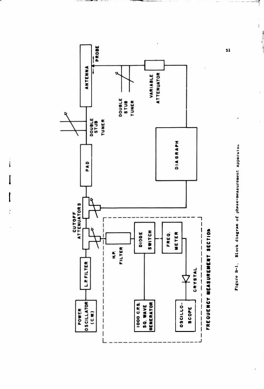
B-l Block diagram of phase-measurement apparatus 5^

B-2 Laboratory equipment connected for phase measurements 52

B-3 Block diagram of amplitude-measurement apparatus 54

B-4 Block diagram of impedance-measurement apparatus 55

MM mma

r»

ACKNOWLEDGEMENT

The authors acknowledge with thanks the work of Henry Hegener, Werner Lain,

Sam Kuo, and Edward McBride, student technicians in the Antenna Laboratory.

L

1. INTRODUCTION

Research on frequency-independent antennas took a giant step forward with

the introduction of the "angle concept" by Rumsey in 1954. This principle

states that a radiating structure can feature patterns and input impedances

that are independent of frequency, provided that its geometry is such that it

can be described in terms of angles instead of linear dimensions. In the years

that followed, this principle was applied in many different ways to produce an-

tennas of widely varying configurations.

Common to all such designs, however, is a basic limitation on size: if the

antenna is to operate at any given frequency, some dimension of the structure is

of the order of one-half of a free-space wavelength at that frequency. Therefore

a broadband antenna, the low-frequency limit of which is, say, three megacycles,

has to be quite large. This size requirement may not be a serious prof em in a

fixed, ground-based installation where a lot of land is available. On shipboard,

however, the problem becomes imporcant. Practical frequency-independent designs

are, to some extent, directional in their radiation characteristics; therefore it

is desirable to mount a shipboard antenna so that it can be rotated. A low-fre-

quency antenna would thus require a large, unobstructed circular area if it were

mounted near the deck of the ship. If it were mounted on top of a mast, its

weight, rigidity, and support would become a problem. A need exists, therefore,

for a size-reduced frequency-independent antenna array.

The first problem is to determine which type of frequency-independent design

best lends itself to some means of size reduction. One class of such antennas

features a geometry which is repeated periodically with the logarithm of distance

from the apex of the structure; these are called "log-periodic" structures. Isbell,'

in 1959, replaced the sheet-metal teeth on one of these log-periodic structures

with conventional half-wave dipoles; thus the log-periodic dipole array was created.

Now a very popular antenna, it was the first applicatioi. of the log-periodic

principle to an array of conventional radiating elements. Several ways of

reducing the resonant length of a dipole are known, and have been used for many

years. Therefore it was decided that the log-periodic dipole (LPD) array would be

the starting point for Ihj size-reduction program.

The most complete analysis and design procedure to date lor an LPD is by 3

Carrel. His paper outlines the history of LPD development, gives a thorough

description of its construction and operation, analyzes the antenna mathematically,

n:-„ ^5« ■T . ..'■"

and provides a complete set of design charts for those who want to build their

own. It has been the basis of all of the work discussed In this chapter, and

it will be referred to in suceeding sections.

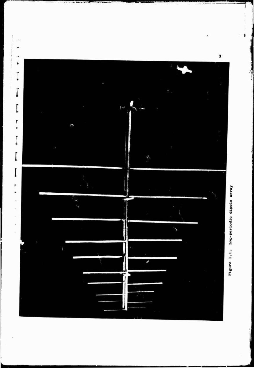
Figure 1,1 is a photograph of of an LPD array, built for testing in the

Antenna Laboratory. The coaxial cable, through which the antenna is fed, trav-

els through one of the feeder tubes to the small end of the antenna; it is at

this point that the antenna is actually fed. Here the wave Is applied to the

feeder, the twin-wire transmission line which runs to the shorting block behind

the longest dipole. The wave travels down the feeder, away from the feedpoint, past

those dipoles which are too short to be resonant at the applied frequency. The

section of the antenna which contains these dipoles is called the- "transmission

region' Beyond the transmission region is the 'active region", the region con-

taining those dipoles which are resonunt at frequencies In the neighborhood of

the applied frequency. In the active region, the energy in the feeder wave is

radiated by the dipoles. If the active region efficiency is high, there is prac-

tically no energy left on the feeder beyond the active region, and the remainder

of the antenna, containing dipoles longer than resonant length, is called the

"unexclted region". It is vhe presence of this unexcited region which allows the

antenna to be terminated at any desired length without affecting Its properties

as seen from the feedpoint.

Proper operation of an LPD depends on the dipole currents in the active region

being phased in such a way as to produce radiation back over the feedpoint, of f the

small end of the antenna. A periodic radiating structure, in which radiation oc-

curs in the direction opposite to that of the exciting (feeder) wave, is said to be

a backfire" radiator. Therefore the term "backfire" is used to describe the proper

mode of operation of an LPD, even though the radiation is actually "endfire" in

terms uf what is usually defined as the "front end' of the antenna, i.e., the end

containing tbe feedpoint

In addition to the dipole-length problem for an LPD at low frequencies, there

is a requirement on boom length (feeder length); directivity suffers if the antenna

is made too short for a given operating bandwidth Although an array that is size-

reduced in one direction only may be quite useful, overall size reduction would re-

quire reduction in both dipole lengths and boom length For this reason, while

primary emphasis is given in this report to dipole shortening, the boom-length

problem is brought in wherever it is applicable. It is worth noting that the

^MMflM^ ^^tta

— ■^ 1

I I

L

—^ mm* ■[■■■■^i n ■ i M

|

radiation pattern of a short dipole is nearly the same as that of a half-wavelength

dipole, therefore dipole length alone should have very little effect on directivity

Succeeding sections of this chapter describe the work done on size reduction

of LPD arrays. Section 1,1 discusses the method used for dipole shortening, and

describes the models used for laboratory testing. Section 1 2 presents the results

of this testing, including efforts towards optimization of the performance of size-

reduced arrays. Section 1.3 describes a type of antenna which combines a conven-

tional LPD with a size-reduced LPD. Data on its performance are presented, toget-

her with a discussion of possible ways of improving it All experimental results

are summarized in Section 1,4 and the capabilities and usefulness of size-reduced

arrays are discussed. Included in the References is a brief review of each of the

references cited in this chapter.

1.1 Dipole Length Reduction and the Log-Periodic Helical Dipole Array

The method chosen for shortening the dlpoles in the LFD array is to replace

them with normal-mode helical dlpoles By the proper choice uf pitch angle and

other helix parameters, a helical dipole may be made to resonate at a frequency

much lower than the frequency for which the dipole is a half-wavelength long.

This method was chosen in preference to inductive base-loading because of

its higher efficiency, and in preference to capacitive end-loading because of the

fact that such end-loading would require a lot of weight hanging out on the ends

of each dipole Dielectnc-loading of the entire array is impractical at low fre-

quencies, The helical dipole also features a uniform geometry which simplifies the

construction

In the following paragraphs are found a brief discussion of helical dipoles

and their characteristics, and a description of the 1 oganthmical ly-penodic

helical dipole array (LPHDA)

111 Normal-Mode Helical Dipoles

The normal-mode helical dipole differs from the more common axial-mode or

helical beam antenna in that its diameter is on the order of one-tenth wavelength

cr less at the frequency of operation. Its radiation pattern is similar to that

of a linear half-wave dipole. Detailed analyses have been made by such authors

as Wheeler, Kraus, Kandoian and Sichak, and Li

In Figure 1 2 are sketched two dipoles. one a half-wave linear dipole, the

other a helical dipole. The degree of shortening of the helical dipole compared

■^A^^^fa^A*

■UM»«!?

4

LINEAR HALF-WAVE DIPOLE

8-=-

HELICAL HALF-WAVE DIPOLE

Figure 1.2. Linear and helical dipoles

-JT- ' -

to the linear one is denoted by the factor s, 0^ s^ 1. As a very rough first

approximation, it may bo assumed that a wave travels down the helix with the

velocity of light, but in the direction of the helical path described by the

wire. Thus the phase velocity in the direction of the helix axis is lower than

that of free space, and is related to the ratio of pitcn p to diameter D Ac-

cordingly, the "guide wavelength" \g, i.c , the wavelength in the axial direc-

tion, is less than the free-space wavelength, \ The resonant length of the

helical dipole would then be one-half of a guide wavelength, but less than half

of a free-space wavelength, resonant length = ^g/2 - s \/2

In order to make any use of helical dipoles, one must know which dipole

dimensions will result in a specified resonant frequency and a specified shor-

teinlng factor s The approximation used above, which says essentially that

the total length of wire in the dipole should be - when unwound, is not satis-

factory except as a starting point for a cut-and-try method of dipole design 6 7

Existing design data ' do not take into account wire size, for example, but

wire size was found (in measurements on helical dipoles and monopoles) to have

a major effect on resonant frequency. In order to provide some more useful de-

sign data, a number of measurements were performed on helical dipoles. The re-

sults of these measurements are discussed in Appendix A

There are several reasons why tho use of helical dipoles in place of linear

dipoles would be expected to change the performance of the array. The radiation

resistance of a helical dipole drops as s is reduced below unity. In a log-

penodic array the active region efficiency is somewhat dependent on the relation-

ship between dipole impedance and feeder impedance, therefore it would be expec-

ted that the substitution of helical dipoles would change the active region

efficiency, and therefore directivity, end effect, etc. Mutual impedances be-

tween dipoles in the array would also be expected to differ from those in an

array of linear dipoles. mutual impedances have a similar effect on 1PD perfor-

mance.

Unlike a linear dipole, the helical dipole produces el 1 iptically-polarized

radiation, but in the range of dipole parameters used in this investigation this

effect was found to be quite small and the polarization nearly linear

Underlying the entire idea of antenna size reduction are certain basic rules

which make it impossible to combine in one antenna high efficiency and gain with

8 9 small size in wavelengths. '

These considerations lead one to exptct a certain degree of deterioration in

the performance of the LPHDA as dipole lenjths are reduced. A major purpose of

this investigation has been to determine to what degree one must compromise in

return for obtaining a narrower array.

1.1.2 The Log-Periodic Helical Dipole Array

Except for the dipo'es themselves, the LPHDA is very similar to the conven-

tional LPD array. The effective 180-degree twist in the feeder from one dipole

to the next, the construction of the feed point, the use of a coaxial cable

through one side of the feeder to drive the antenna, etc., are all in accordance

with conventional LPD design.

Figure 1.3a illustrates the parameters used to describe the array. These cor-

respond to the parameters used in LPD design, except that the spacing factor O is

now defined in terms of the free-space wavelength, Xn, at the resonant frequency

of the n dipole. instead of the length of the n dipole. Figure 1.3b shows the

way in which the dipoles are connected to the feeder.

The method of construction of laboratory models was dictated by measurement

requirements. These are discussed in Appendix B, The feed cables for the LPHDA

models ^nd the LPD models built for comparison purposes) were made from RC-141

cable, a teflon-dielectnc type similar in size to RG-58. Silver tubing, just

large enough to contain RG-141 cable with its outer fiberglass cover removed, was

used for the feeders. The dipoles themselves were wound with copper or tinned

copper wire on cylindrical polystyrene rods. The wire was soldered to the feeder,

usually with conventional tin-lead solder, and the polystyrene rods were glued to

the feeder for mechanical support (except for the variable - O models). All helix

dimensions were scaled by the factor T as closely as standard A.W.G. wire sizes

permitted. A shorting plate was soldered across the rear end of the feeder, at

a distance K/8 behind the longest dipole. A cut-and-try technique was used to de-

sign the dipoles themselves to make them resonant at the desired frequencies.

In Section 1,4 of this chapter some comments are made on the construction of

LPHDA antennas for operation in und above ^he HF (3 to 30 Mc) range,

1,2 Experimental Investigations and Results

Extensive experimental work on LPD antennas, performed in the Antenna Labora-

tory, has produced a wealth of data with which LPHDA models could be compared. For

this reason, the LPHDA experimental investigations have been based on previous (and

U» L-. T^am^^i

DIRECTION OF

^ t R s I ^ s h?-, N h ÜJ J s

MAXIMUM RADIATION ir

s s

s S s s

rs

s

N S S s s

s

S

_ i Ir

n+i

Xn

n*i Xfi ~Xn^| 'n s S

Figure 1.3a. Parameters of an LPHDA.

HEUCAL DIPOLES

CHARACTERISTIC \ A

IMPEDANCE « 2o Xv

Figure 1.3b. Feeder and dipole detail of an LPHDA.

9

current) LPD measurements. A description of the techniques used, together with

block diagrams of the test equipment connections, is found in Appendix B.

Wherever directivity is mentioned in this report, it was calculated from the 5

approximate formula~ 41,263

Directivity in decibels = 10 log (BW) (BW) E H

where (BW)E and (BW)8

are the half-power beamwidths, in degrees, in the E-plane

and the H-plane, respectively. Whenever values of VSWR are mentioned, theEe are

maximum values of VSWR with respect to the mean value of input impedance over the

entire given frequency range (although individual impedance points that are isola­

ted from the remainder of the points on the Smith Chart are occasionally discarded

from t he VSWR calculation).

1.2.1 Active Region Efficiency vs. s

It is clear that a very small degree of dipole shortening (s close to 1)

would result in an array the performance of which is nearly the same as that of

an ordinary LPD. But such an array would be of no value where size reduction is

an important factor. The first problem, then, was to determine a range of values

of s in which both satisfactory performance and appreciable size reductions could

be obtained.

Two pattern models were built, each uniformly periodic; that is, the scale

factor T was unity, all dipoles resonated at the same frequency, and the dipoles

were spaced uni f ormly along the feeder. Such an antenna is not a broadband de­

vice, but it is ~seful in predicting the performance of broadband, log-periodic

arrays in certain respects; Section 1.2.4 discusses its properties in greater

detail.

Each of the uni formly-periodic models contained five dipoles. The same

dipole spacing was used on each, and their feeders were of equal length and

open-circuited at the ends opposite the feedpoints. Their feeder characteristic

impedances, Z , could be varied. The difference between these models was that 0

the shortening factor s was equal to 0.26 on the first model, and 0.57 on the

second.

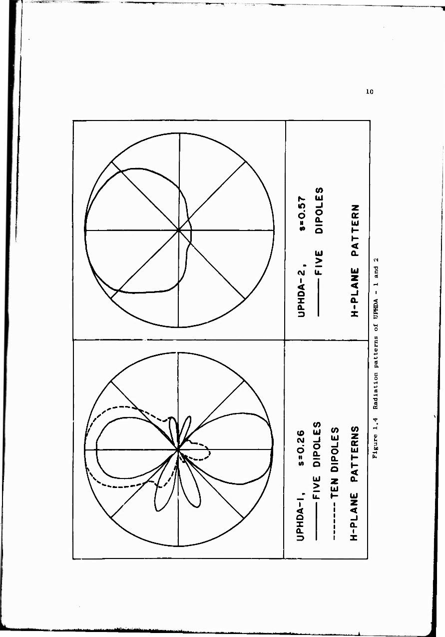
Figurel.4 shows, in solid lines, the far-field radiation patterns of these

two antennas. While the second model (s = 0.57) exhibited undirectional backfire

radiation at the dipole resonant frequency, the first model (s = 0.26) featured a

strongly bidirectional pattern. Only whun five more dipoles were added to the

10

a> 1/^ // \ 1 N Ul f \ «0.5

IPO

L

UJ II -w^ 1 1

• Q 1- 1- < u Q-

> • - 0«

M Ü. UJ | z

v^^ ^ < < ^w^ ^r o -1 z Q.

Q. 1 3

\/C ~^X 1 s* ""%> Jr ^m^^^m^^^m>_ \ / * _>J^ —. yk jr ^^^^^^^^ ^^^^^^^ \ 1 / / ^^*' ^»^ *»^T\ rl X^^^ ^V\

(0 // / ^^\ \l Is^ I (0 UJ (O W

1 ( ( >l^--v J CSi -J

ö ° UJ z

1 1 t .^^V^ 1 1 o l \ Jr i\&£m"'' 1 H Z ';' OL 1-

1 W ^^//fli v^ yf M O o < \"—sy \ \ x— / UJ

> UJ Q.

\ / \ \ \ \ / - Ü. H UJ \ / \J \J \ / ^ i 1 z \s \s < <

^r o J ^/^ z Q- ^^ | Q- 1

.—^^ ! 3

I

j

11

first array, giving it a total of ten dipoles, did it exhibit backfire radiation

(broken line in Figure 1,4). Further pattern measurements, taken at different

values of Z , all showed the same effect, o

These results illustrate a strong dependence of the efficiency of the active

region upon the value of s. In the s = 0.26 model, each of the original five

dipoles radiated relatively little of the energy that was propagated towards them

along the feeder. The remainder of the energy continued to the rear end of the

feeder, and was reflected back towards the feed point. This reflected signal ex-

cited the dipoles once again, producing strong radiation in a direction opposite

to that produced by the incident feeder signal; hence the bidirectional pattern.

A log-periodic array built with such a low value of s would therefore suffer from

strong end-effect and poor front-to-back ratio, unless the scale factor T were

very close to unity. Such a T would lead to an extremely long antenna for any

appreciable operating bandwidth.

For this reason, it was decided that a value of s in the range 0.5 to 0.6

would be used in subsequent size-reduced models. This should be kept in mind as

experimental results in the following sections are studied; the levels of pei—

formance obtained with such LPHDA models could not necessarily be expected to

hold for lower values of s. Further work would be necessary in order to determine

favorable design parameters for arrays with smaller s.

1.2.2 Direct Comparison of Arrays of Linear and Helical Dipoles

To gain further insight into the effect of dipole shortening, two pairs

of log-periodic arrays were built. In each pair, the models were identical except

that one was built with linear dipoles while the other had helical dipoles. The

first pair, LPD-1 and LPHDA-1, was based on Carrel's "optimum" design for 9.5 db

directivity; the second pair, LPD-2 and LPHDA-2, was based on minimum boom length 3

for 9 db directivity. It was discovered, after construction and testing of the

first pair, that the helical dipole design had been in error and that the frequency

range of LPHDA-1 was different from ihat of LPD-1; therefore a direct comparison

could not be made. The dipoles in LPHDA-2, however, were designed more carefully.

It was on this second pair of antennas that the data presented here were measured.

The shortening factor for LPHDA-2 was 0.54.

Figure i.5 shows the far-field H-plane radiation patterns of this pair oi an-

tennas at four different frequencies. The patterns of LW-2, represented by dashed

lines, are quite consistent over the entire frequency range for which the antenna

L

12

837 Mc

LPD-2

400-1000 Mc

1033 Mc

<r « 0.10

LPHDA-2 (fO.Ö^

T- 0.90

H-PLANE PATTERNS

FiKure 1.5. Radiation patterns of LPD - 2 and LPHDA - 2

13

was built (400 to 1000 Mc). By contrast, the patterns of LPHDA-2 (solid lines)

deteriorate quite noticeably at the ends of the frequency range (the 400 and 1033

megacycle patterns). This result, like the result discussed in Section 1.2.1,

shows that the active region on the LPHDA includes a larger number of dipoles

than does the active region on the corresponding LPD.

The 610 Mc pattern is typical of the mid-range performance of the LPHDA. It

is seen that both directivity and front-to-back ratio suffer somewhat by compari-

son with the LPD.

Figure 1.6 illustrates the variation with frequency of the input impedances

of the antennas at their feed-points. Impedance readings were taken at three -1/3 f -2/3 -1

frequencies per log-period; that is, f , T ' n, T * f , T f = f ,, etc., ' n' ' n' n n+l' '

where f is the resonant frequency of the n dipole. The impedance shown by the n

individual dots on the Smith Chart are those of the LPHDA, from 400 to 1000 Mc.

The ciicle on the chart encloses all of the LPD impedances over the same frequency

range. The VSWR with respect to met-n input impedance varies as follows:

LPD: VSWR =1.5, 400-1000 Mc.

LPHDA; VSWR = 4.85, 400-1000 Mc.

VSWR =3.2, 400-753 Mc,

Figure 6 does not show the direction of movement of the impedance on the chart

as frequency is changed. It is remarked here that the impedance displayed the or-

derly, clockwise progression, with increasing frequency^that is characteristic of

log-periodic arrays.

All of the data obtained on this pair of antennas may be summarized as follows:

the LPHDA, built with the same design parameters as the LPO but with s equal to 0,54,

featured an operating bandwidth about 65^> as wide as that of the LPD, an average

directivity of about 6.4 db compared to 9 db for the LPD, an average front-to-back

ratio of 15.4 db compared to a minimum of 20 db for the LPD, and the comparisori of

VSWR given above.

This degradation in performance, of course, was anticiapted from the discus-

sion in Section 1.1.1. But there is no reason to assume that optimum performance

in an LPHDA should result from the same design parameters as those which lead to

optimum performance in an LPD. The next step, therefore, was to determine the

degree to which LPHDA performance could be improved by changing the values of

various design parameters.

■»'^

1/

LPD-2 ond LPHOA-2 (••0.54)

<r " 0.10 T«0.90 400- 1000 Mc Point Freq. Point Freq. Point Freq.

1 400 Mc. 11 568 Mc. 21 809 Mc 2 414 12 589 22 837 3 429 13 610 23 866 4 444 14 631 24 897 5 460 15 655 25 929 6 477 16 678 26 962 7 494 17 702 27 998 8 511 18 727 28 1033 9 530 19 753 29 1069

10 549 20 779

Figure 1.6. Input impedance of LPD-2 and LPHDA -2

— ■ - i

15

1,2.3 LPHDA Performance vs. T, a. and Z ' o

The goal in this investigation was to determine which values of T, (7, and

Z lead to optimum performance of an LPHDA with s = 0.5, in terms of directi- o '

tivity, VSWR, and boom length.

LPHDA models 3, 4, and 5 were built to cover a 400-800 Mc frequency range.

These models featured a feeder impedance Z of 100 ohms, a shortening factor s

of 0.54, and scale factor T of 0 90, 0.92, and 0.95, respectively. Two of these

arrays are shown in Figures 1.7 and 1.8. The dipole core rods were not glued to the

feeders, by unsoldering the wires from the feeder one could move the dipoles to

any desired location on the feeder. The shortening plate behind the longest

dipole could be unsoldered and moved. Small plastic clamps held the feeder to

its proper spacing. Measurements of input impedance and far-field patterns, as

functions of frequency, were made for several different values of 0 on each

model.

In Figure 1.9 are shown the results of these measurements, plotted in terms of

VSWR. It will be noticed that each of the three antennas featured a value of Q

that was "optimum", i.e., that produced the lowest VSWR. Design "A" in Figure 1.9,

with T = 0 90 and (T = 0 16, gave the lowest VSWR, just under 2. But since boom

length is directly proportional to CT, design "A" resulted in quite a long antenna.

Design "B", the T = 0.92 model with Q - 0.07, performed almost as well in terms of

VSWR (2 2), and was much shorter and more compact. Design "C" with T = 0.95 and

(7 - 0 05 featured a VSWR of about 2.5, but it appears to be the most compact array.

In reality, however, it is longer than design "B", because the increase in T more

than offsets the decrease in O. Thus from the standpoint of VSWR and boom length,

the best design of these three appears to be design "B". Figure 1.10 shows the im-

pedance pattern for design "B", and Figure 1J.1 shows, for comparison, the consi-

derably poorer pattern for the T = 0.90 array at ff - 0.07.

Figure 1.12 shows ihe radiation patterns of the design "B" model. Directivity

is about 6.5 db, and front-to-back ratio averages 15 db from 400 to'800 Mc and 19

db from 514 to 800 Mc. There were only minor variations in the radiation patterns

of the three variable - 0 models as O was changed, but in general the best patterns

and the best VSWR were found at approximately the same O values. For all models,

the front-to-back ratio was rather poor over the lowest log-period of frequency;

thit> effect was mentioned earlier in connection with LPHDA-2. At the high-frequency

^i I,

16

co

1

u o a u o

3

0) u 3 bO

^Mtf^^M^lteMM

17

i

4)

S

o *J A t. 0

Si

5

0) u 3

«

18

•O ♦ IO CM

33Nva3dWJ NV3W Oi lD3dSad HUM dMSA

o I-

o z o to

c (3

>

£

05

3 tx

•M^i^MMt^^

LPHDA - 4a (S« 0.54)

o" ■ 0.07 T« 0.92 Point Freq.

1 414 Mc 2 429 3 444 4 460 5 477 6 494 7 511 8 530 9 549 10 568 11 589 12 610

Figure 1.10. Input

414-800 Mc

Point Freq.

13 631 Mc 14 655 15 678 16 702 17 727 18 753 19 779 20 809 21 837 22 866 23 897

Input impedance of LPHDA design B

"Wü""^^^-*-

20

LPHDA-3a (8.0.54)

<r.0.07 T.0.90 414-800 Mc Point Freq.

1 400 Mc. 2 414 3 429 4 444 5 460 6 477 7 494 8 511 9 530

10 549 11 568

Figure 1.11. Input imc

Point Freq.

12 13 14 15 16 17 18 19 20 21

589 610 631 655 678 702 727 753 779 866

Input impedance of poor LPHDA design

- —»- ^^-- - ■-

21

400 Mc 473 Mc

558 Mc 660 Mc

780 Mc 922 Mc

LPHDA - 4 (r • .07

H - PLANE PATTERNS

T ■ 92 S-.54

FiRurc 1.12. Radiation patterns of LPHDA design "B'

"T -T

I

*

22

end, however, the patterns held up quite well all the way to 800 megacycles

It is difficult to compare the boom length ol design "'B" with that of an

LPD of the same directivity, because existing LPD design charts do not give

complete figures for directivities lower than about 7 5 db. It is clear that the

LPD would be somewhat shorter. It is also worthwhile to note that the insertion

of T and 0 for design "B" into the LPD design charts gives a directivity of about

8.8 db

In order to investigate the effect of Z , a new model (LPHDA-6) was built o

in which Z could be varied up to a maximum of 275 ohms. Design "B" was used for

T and <7 Impedance measurements, at different values of Z . showed a rather dis- ' o'

tinct improvement in VSWR at Z = 250 ohms, for which the impedance pattern is

shown in Figure 1 13 The VS^ here is about 1 95. it increased to 2.33 and 2 31

at Z = 230 and 275 ohms, respectively. Pattern measurements showed results verv o

similar to those obtained with Z = 100 ohms the directivity was about 6,5 db o '

and the front-to-back ratio averaged 15.27 db from 400 to 800 Mc and 20 2 db from

514 to 800 Mc.

Measurements are now under way on another variable - Z model, patterned af- o

ter design "B", hut with a capability of Z values considerably higher than 250

ohms ,

1 2.4 k- ß Characteristics of Lniform Arrays

At any given frequency within the operating range of a log-periodic array,

the active region of this array may be approximated by a uniformly periodic array

of dipoles which are resonant at that frequency Moving along the LP array, from

the transmission region through the active region and into the unexcited region,

is equivalent to changing the frequency of the signal applied to the IP array,

trom a frequency below dipole resonance to a frequency above dipole resonance

For this reason, UP arrays have been used extensively as laboratory mode'1--, es-

pecially f;)r the study of k-ß characteristics

The k-P characteristic of a radiating periodic structure is a convenient way

uf relating the excitations of the radiating elements (in this case, the dipole

currents) to the far-field radiation pattern of the structure. It has been studied

extensively, both theoretically and experimentally. ' Although its full mean

ing is not yet completely understood, it was felt that it would be of interest to

obtain experimentally the k-ß diagram for a uniformly periodic helical dipole array

■*■'■ • ■"

LPHDA-60 (t-0.54)

<r«0.07 T«0.92

Z#-250 a 400- 800 Mc

Point Freq. Point Freq. Point Freq.

1 400 Mc 11 528 Mc. 21 698 Mc 2 411 12 543 22 717 3 423 13 558 ^.1 737 4 435 14 574 24 759 5 447 15 590 25 780 6 460 16 607 26 801 7 473 17 624 27 825 8 486 18 642 28 896 9 500 19 660 29 922 10 514 20 678

Figure 1.13. Input impedance of LPHDA - 6a at optinum Z

24

(UPHDA) for purposes of comparison.

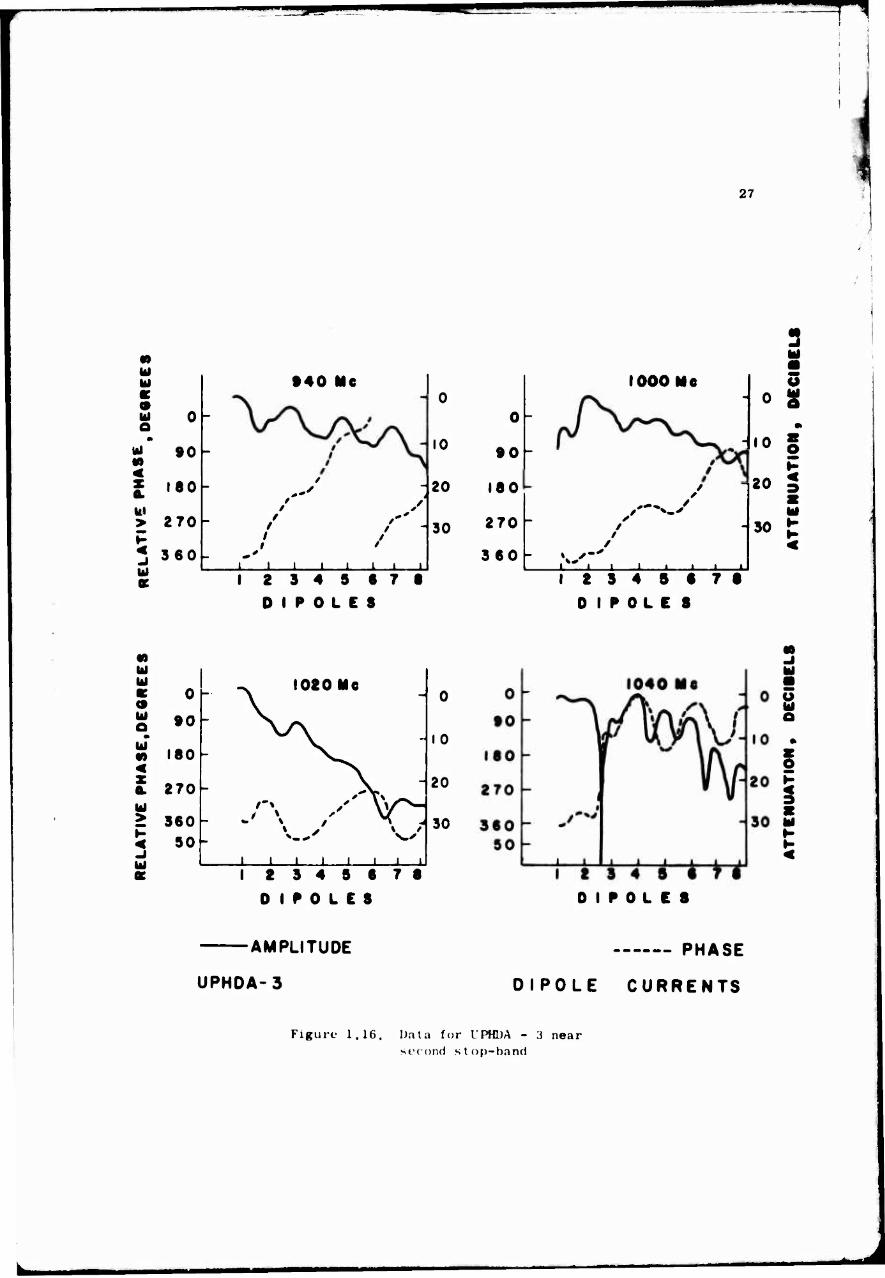
UPHDA-3, shown in Figure 1.14^ was constructed for this measurement It

contained 14 identical dipoles, equally spaced with 0 - 0,087 and s = 0.53.

Appendix B discusses the method of probing the antenna so that the measured

signal was proportional to the dipole currents. Relative amplitude and phase

of the probe signal were measured at many frequencies as a function of dis-

tance along the feeder. Figures 1,15 and 1.16 show a representative sampling

of the data obtained. The resulting k-^ diagram, including attenuation vs k,

is shown in Figure 1.17.

The k-ß diagram is often plotted in terms of ka vs. Pa, where a is the

period" of the structure, i.e., th».1 length of one "cell" or the distance from 271

nd one dipole to the next Here, k = T- , the free-space phase constant, a o

ß = r— . the phase constant along the structure. Thus it is clear that plot- \

K a a J ting r— vs. r— , as in Figure 1.17, is equivalent to plotting ka vs, Pa except K K

o g a

for a constant factor 277. The T— coordinate of each point was calculated by g

making a straight-line approximation to the phase curve at each frequency,

wherever possible (for example, 300 Mc in Figure 1.15) The attenuation per

cell was calculated by making a straight-line approximation to the amplitude

curve Not all of the phase curves could be translated into points on the k-ß

plot For example, at 393 Mc (Figure 1.15) and at 1020 and 1040 Mc (Figure 1 16).

straight-line approximations to the phase curves could not be made. This effect

is common to such measurements, it can be caused by more than one mode being pre-

dominant on the structure at one time. For these frequencies, points were not

plotted on the k-P diagram

Figure 1 17 is similar in form to diagrams derived from measurements on

arrays of linear dipoles The one important difference is that the maximum value

of attenuation per cell on the L'PHDA is about 6 db, while values of 20 db or su

have been obtained in arrays of linear dipoles. This important result agrees with

the concept of a wider active region on the LPHDA, the effects of which were seen

in IPHDA-l (Section 1 2.1) and LPHDA-2 vs LPD-2 (Section 1 2.2)

- *m

TH

^1 25

n

0)

B

o *-> cd u o

2

3

26

1

v

1 - m 1 in i I ct

o 300 Mc

111

f

o *

hi 0

/ m < 90

'' / X a. in 180 . r / >

■ / P 270 <

/ hi ae

360 ^ . . ./ . . .

1 2 3 4 5 6 7 ~8 0 1 P 0 L E S

> 2 3 4 S 6 7 6 0 I P 0 L E $

w w

ill

Si 12 3 4 8 6 7 8

0 I P 0 L E 8

AMPLITUDE

UPHDA-3

0

90

180

270

360

393 Me

2 3 4 8 8 7 8 0 I P 0 L E 8

PHASE

DIPOLE CURRENTS

Figure 1.15. Data for UPHDA

stop-band 3 near first

**fe^tfM^tei

27

toi Q

III

0

90

180 itl > 270

360 -

940 Me

,*' .*■»

J I I I I I L

0 0

IG 90

20 180

30 270

360

ce 1 2 3 4 9 8 7 8 0 1 P 0 L C 8

M in IM

0 -^ 1020 Me 0

<f V in o 90 \y\ • Ul V. 10 M 180 ^^^ < ^^v X 0. 270 ^•^p*

20

in r\ s \y^- > 360

SO 30

J III i i i i i i i i

1 2 3 4 9 6 7 8

D 1 P 0 L C 8

AMPLITUDE

l JPHDA-3

1000 Me

^^

•^^

J I U L.

- 0

- 10

20

30

I 2 3 4 S 8 7 8

0 I P 0L C 8

3 hl

5 8

O

hl

.1 hl

S

O

3 S hl

0 I P 0 L E 8

PHASE

DIPOLE CURRENTS

Figure 1.16. Data for L'PHDA - 3 near second stop-band

i in m m

I N fr 2 — (o oJT n *&

' ■R ^1

>

5 no

N

PE

R

p ^ '^ Np!3 o ♦ 6 lu kj * K ig

i o

"is

28

J

a c n

3 C 0

c in cj

ta a

T3 Ö

hifctMg

29

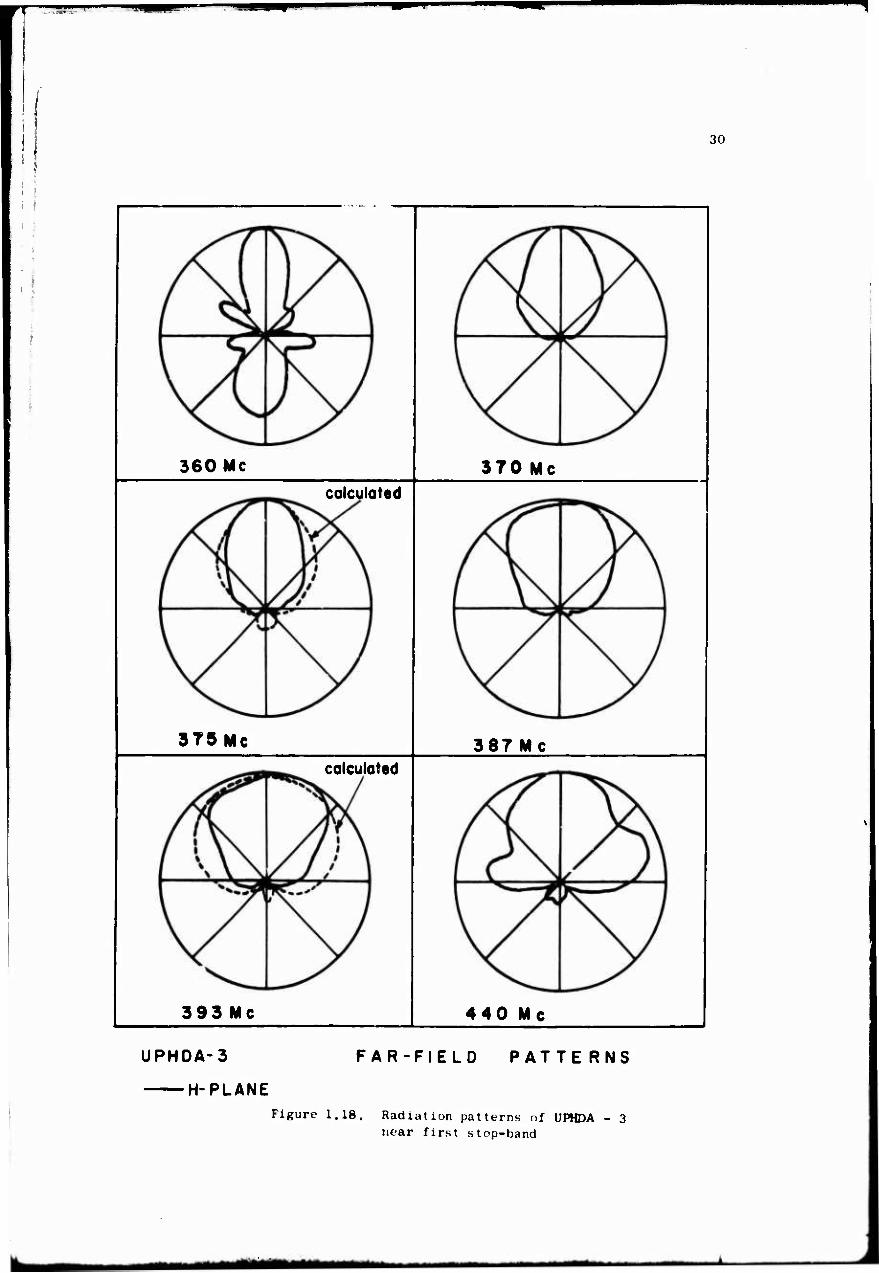
Measured far-field radiation patterns, shown in Figures 1.18 and 1.19 show

excellent agreement with the k-ß plot. The low values of attenuation per cell

at 360, 800, 900 , and 920 megacycles produce the bidirectional form of the pat-

terns at these frequencies, as was the case with UPHDA-1 with five dipoles.

Maximum attenuation per cell in the first stopband occurs at k-P points fairly

close to the backfire region, in the second stopband maximum attenuation does

not occur until the beam has split considerabl v toward-, broadside. This, plus

the fact that the second stopband occurs at a frequency less than three times

the frequency of the first stopband, indicates that further study might be

necessary to achieve good operation in the 3/2 wavelength mode.

Figure 1.18 shows calculated patterns in addition to the measured ones at

375 and 393 megacycles. These calculations were based on the measured dipole

current amplitudes and phases, in an attempt to evaluate the accuracy of these

measurements The results indicate an acceptable degree of reliability for the

measured data It should be remembered that the pattern measurements, taken on

existing facilities at the Antenna Laboratory, are most accurate at frequencies

above 500 megacycles.

1.3 Log-Periodic Mixed Dipole Arrays

In the preceding sections, the work described was Jevoted to optimizing the

performance of an LPHDA. This section describes the investigations of a more

practical design, which combines the size reduction of an LPHDA with the perfor-

mance of an LPD. The log-periodic mixed dipole array (LPMDA) is based on the

idea that in a broadband antenna the need for size reduction is felt most strongly

in the longer (lower-frequency) dipoles only, the shorter dipoles may just as well

be linear ones Over most of the i requency rangf, 'hen, the antenna would perform

with the higher directivity and more uniform impedance characteristics of an LPD,

and the sacrifice in performance inherent in an array of helical dipoles would be

felt only in the first few log-periods at the low-frequency end of the band.

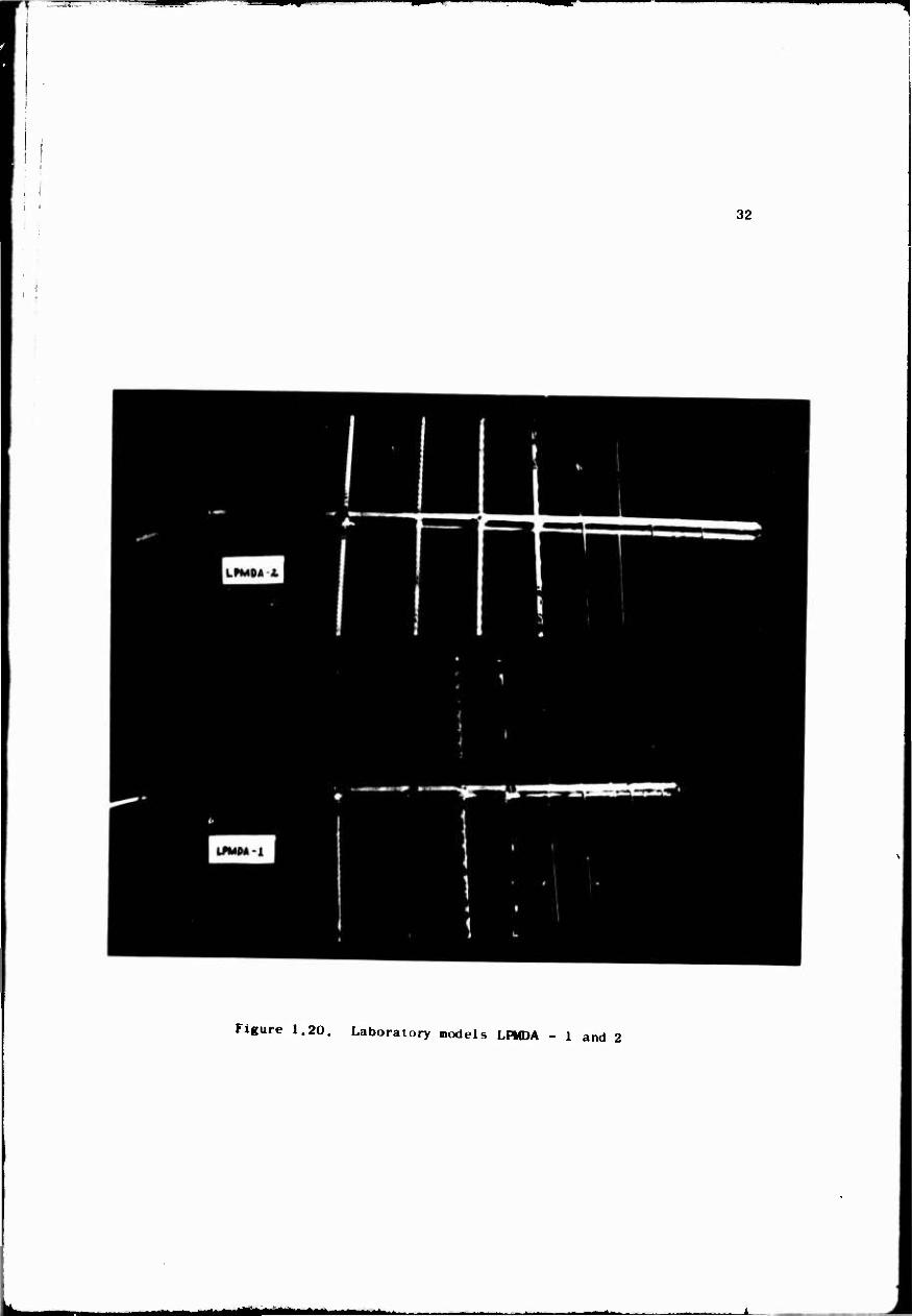
Figure 1,20 is a photograph of the two mixed arrays that were built and tested,

Those models are 1/70-scale models of 6-25 megacycle arrays (frequency range for

models: 420-1750 Mc). The first four dipoles on each model are helical, the rest

are linear. Unlike in previous models, the holical dipoles are not scaled in

length. For the first dipole, 8=05, for the second, third, and fourth dipoles, -1 -2 -3

s increases to 0.5 T , Ü 5 T , and 0,5 T , respectively. Thus all four helical

dJpoles are the same length, but = is adjusted for each so inat the resonant

;

■

«■

30

360 Mc 370 Mc calculated

375Mc 387 Mc calculated

393 Mc 440 Mc

UPHDA-3 FAR-FIELD PATTERNS

H-PLANE Figure 1.18. Radialion patterns of UPHDA

near first stop-band

MM MM I^M^.

■TFP T^

31

600 Mc 900 Mc

9 2 0 M c 95 0 Mc

970 Mc 000 Mc

UPHDA-3

H-PLANE

Figure 1.19.

F AR-F IELD PATTERNS

E-PLANE

Radiation patterns of UPHOA - 3 near second stop-band

32

Figure 1.20. Laboratory models LPMDA - 1 and 2

^^^toMMHa^^M,

33

frequencies scale log-periodically from one to the next. This provides, in

effect, a gradual transition from helical to linear dipoles.

Other design parameters were;

LPMDA-1 . T = 0 825, CT = 0,06, O- = 36°, Z = 135 ' o

LPMDA-2 T - 0 85, 0 = Ü 07, a = 28°, Z = 135 ' o

These are far from the optimum parameters found for the LPHDA; they were

chosen to represent a useful and reasonably compact LPD design.

Impedance measurements resulted in data such as shown for LPMDA-1 in

Figure 1.21. The sixteen points shown are spaced evenl> through the first four

log-periods. The point labelled "f " is at the resonant frequency of the first

helical dipole; the next three points connected to it by the line correspond to •1/4. ,-1/2. . T-3/4

frequencies 'r 1/4, T-l/2, fj. T il, anc f . The next point is the one labelled

"f ", etc. It will be noticed that as frequency is increased the impedance pat-

tern, with the exception of the point labelled "f ", spirals inward towards a

progressively lower VSWR. Impedance points at frequency f and above are omitted

for clarity, but they are clustered around the point 1 .5 •* j 0 with a VSWR of less

than 2.

Figure 1.22 shows some of the radiation patterns of this same antenna. Again,

with the "Xception ol the H-plane pattern at f performance improves progressively

as frequency is increased: this time in terms of directivity and front-to-back

ratio (note particularly the E-plane patterns). Above frequency f , the pattern

remained quite uniform

These results may be summarized as follows;

Freq Range

1 " f2

2 3

- f 4 5

_ and above

VSWR

3 58

2 27

2 11

1 91

1 91

Front-to-Back Ratio

3.36 db

8.22 db

11.69 db

20.28 db

21.5 db minimum

The impedance and pattern at the single frequency f ai omitted from the 4

above table. This seems to be an exceptional point, data at all other frequen-

cies weie well-behaved.

■ ■

34

LPMOA-i: FIRST FOUR LOG-PERIODS

9-0.06 T-0.82S a>360

Figure 1. 21. Input impedance of LPMDA - 1

-^^—— -

35

yS^^. nr\. JT ^F 9 \ ^ä^.

/s\ \ \y\\ fr ^V. ^ Jr \ \ If >^ s* \ \ If \^ s* 11 ll ^ ^1.^ jl

v^-^-^^t A ^/ \^ b

LPMDA-I FAR-FIELD PATTERNS

H-PLANE E-PLANE Figure 1.22. Radiation patterns of LRMDA - 1

36

Model LPMDA-2 behaved in a manner very similar to that of LPMDA-1. In evi­

dence again was the gradual improvement in performance as frequency was raised

toward the range where the linear dipoles become active.

It is appropriate here to comment on the idea of overall size reduction,

i.e., the effect of the 5~ shortening upon the diameter of a clear circular

area which would be required to allow the antenna to be mounted horizontally and

rotated in azimuth. A 6-25 Me log-periodic dipole array, built according to the

values of T and a that were used in LPMDA-2, would require a circular area 28.2

meters in diameter. With dipole shortening of 5~ on the first dipole, etc., as

was done in LPIDA-2, the diameter of the required area reduces to 22 meters, an

overall size reduction of 0.78. The same analysis, applied to arrays with T and

a as used in LPMDA-1, results in a diameter of 25.6 meters for the LPD array, and

17.6 meters for the mixed array, an overall size reduction of 0.6875. These re­

ductions, of course, are based on design parameters tftat are better suited for

linear dipole arrays than for helical dipole arrays. A similar analysis performed

d " h on arrays built according to, say, esign 8 of Section 1.2.3 would result in

considerably higher value for overall size reduction.

Two methods are proposed, whereby the low-frequency performance of LPMDA

antennas might be improved . The first method consists of raising T and decreas­

ing a for the helical elements only. This could be done in such a way as to cause

little or no change in the overall size reduction described above, but the degree

of improvement might be limited. The change in parameters could be made gradually,

as s was changed gradually, or it could be made all at once at the point where the

helical dipole section and the linear dipole section come together. Further ex­

periments would be needed to determine to what extent the operating characteristics

of the antenna could be kept uniform throughout its frequency range.

The second possible method of improving LPMDA performance is actually one

that was suggested by the results of Section 1.2.2: add an extra dipole to the

low-frequency end of the antenna, i.e., design the antenna for a low·-Irequency cut­

off one log-period below the lowest frequency at which the antenna will be used.

This method, of course, lengthens the array and adversely affects the overall size

reduction.

To provide an idea as to the effectiveness of this procedure, LPMDA models 1

and 2 were both measured for impedance with their first helical dipoles removed.

37

In each model, the resulting VSWR was higher, frequency for frequency, than for

the original array. For example, while the original LPMDA-1 measurements re­

sulted in a VSWR of 2.27 from f2

to f3

, the new data gave 2.77 for the same

frequency range and 2.26 for the range f3

to f4

• In general, the performance

of the array with one dipole deleted was similar to that of the original array

at a frequency range one log-period higher.

1.4 Usefulness of Size-Reduced Arrays; Practical Design Considerations

1.4.1 Summary of Data and LPHDA and LPMDA Uses

Results of the data obtained in this investigation may be summarized as

follows:

A. Helical dipoles are useful and practical size-reduced elements

for use in ~ log-periodic array . It is advisable, however, to measure

the resonant frequency of at least one dipole from any given array, and

to adjust its resonant frequency experimentally to the desired value.

The rest of the dipoles in the array may then be designed by scaling

all dimensions from those of the measured dipole by powers ofT.

B. The substitution of helical dipoles for linear ones in an LP

array leads to higher VS\Yk and poorer directivi'.;~. Any given set of

design parameters for an LPHDA produces an antenna whose boom length is

greater than that of an LPD of comparable performance.

C. The active region on an LPHDA is wider (contains more dipoles)

than that of an LPD array. Consequently the operating bandwidth of the

LPHDA is narrower. This effect occurs principally at the low-frequency

end.

D. Perhaps the most practical design for an antenna with a very

large bandwidth is the log-periodic mixed dipole array.

From these characteristics, several conclusions may be drawn concerning

possible ways in which LPHDA or LPMDA antennas may be of value. An antenna

designer who is faced with space limitations may find such an array to suit

38

his needs if he is willing to give up bandwidth. If he needs large bandwidth,

these designs may still be useful if he is willing to sacrifice shortness by

adding an extra log-period or two to the low-frequency end. Or perhaps his

problem is one of mechanical support or rigidity: a long boc.-n on which are

mounted long dipoles could be quite difficult to support rigidly on, say, the

top of a tall mast. Shortened, stiffer dipoles have an obvious advantage here,

even if using them means making the boom longer,

1.4.2 Practical Design Considerations

Once the decision is made to use an LPHDA or LPMDA, some comments are

needed concerning the construction of a low-frequency model — one, for exam-

ple, which would operate in the HF (3-30 Mc) range.

Two important helical dipole parameters are the ratio of helix diameter

("D" in Figure A-2) to length or to free-space wavelength, and the ratio of wire

diameter to helix diameter. The choice of these ratios is somewhat limited: If

D is too small, the dipole will be too flexible and will require excessively

small wire. But if D is too large, the dipole is bulky and heavy, and it will

produce a strong cross-polarization component in its radiation field. For a

given helix diameter, wire which is i oo small will create high resistive losses;

large wire adds weight, makes the helix core smaller and therefore weaker, and

does not give as low a value of S as does a smaller wire, wound to the same

diameter and pitch, Laboratrry models have featured wire size-to-hel ix diameter

ratios between 0.1 and 0.02, and helix diameter-to-length ratios of 0,1 to 0.04.

Within these limits, the specific ratios chosen are not critical.

Polystyrene was chosen for the helix core material in laboratory models be-

cause of its low loss at the high frequencies used for testing the models. For

low-frequency antennas, fiberglass is a widely used material, and would be an

excellent choice for helical dipoles As long as the helix diameter is quite

small compared to its length, the performance of the dipole is affected very lit-

tle by the dielectric properties of the core material; therefore it would not

matter electrically whether the core is made hollow or solid. A hollow fiber-

glass core would probably be both light and sufficiently strong. For the helix

wire, any good conductor cuuld be used. Copper tubing is a common material for

large-diameter conductors. It need not have a round cross section, a strip of

thin sheet material could be used instead of wire or tubing.

^a^

39

In any case, once the materials and parameters are chosen for an LPHDA and

a dipole built and measured, it is important that length, diameter, pitch, and

conductor size are all scaled by the factor T from one dipole to the next in

order that the resonant frequency will be scaled by T also. This is not the case,

however, for the LPMDA, on the models shown in Figure 1.20, only the pitch was

scaled. Dipole length, diameter, and wire size remained constant for all four

helical dipoles. To achieve the proper dipole resonant frequencies, it was found

necessary tu build several dipoles of different pitch, plot their resonant fre-

quencies as a function of pitch, connect the points with a smooth curve, and

then read from the curve the values of pitch needed to give the proper resonant

frequencies for each of the dipoles.

Construction of the feeder on an LPHDA or LPMDA is no different from the con-

struction of jonventional LPD feeders in the same frequency range. The method of

securing the dipoles mechanically to the feeder will be determined by the materials

used, the strength required, and the relative sizes of the pieces to be Joined to-

gether. The presence of a piece of dielectric (the helix core) in and around the

feeder at each dipole location will not have an appreciable effect on the operation

of the feeder, so long as the cores are not excessively large.

1.4.3 Future Work, Conclusions

Research performed on this task to date has indicated a number of areas in

which further work is necessary. Some of these areas were mentioned earlier in

the report; the effect of the feeder Impedance Z , and the optimization of LPMDA

performance in the helical dipole region by changing T, 0, and Z . Studies of the ' ' o

UPHDA k-ß characteristics suggest that it might be possible to increase the gain by

inserting extra phase shift in the feeder between dipoles. A mathematical analysis, 3 11

similar to those performed by Carrel or Mittra and Jones , could help in under-

standing the performance of LPHDA antennas and provide usoful data for design

charts. New facilities to be obtained for the Antenna Labnra'.or1 will permit

moasurements of absolute gain, and thus of overall efficiency

The authors feel that the present work, together with worn on the above items

in the coming year, will make the lug-periodic helical and mixed dipole arrays

useful members of the popular family of frequency-independent antennas.

• Diameter D, as used in this report, is the diameter of the helical path des- cribed by the center of the wire. It is equal to the core diameter plus twice the w i re rad i us .

—^^mm

40

REFERENCES

1. V. H. Rumsey, "Frequency - Independent Antennas", Technical Report No. 20, Antenna Laboratory, University of Illinois, Contract AF 33(616)-3220, 25 October 1957.

The geometry of antennas specified by angles is presented. Observations are made on the theory of convergence of patterns and impedances to fre- quency - independent values. Appendix discusses surfaces for which a rota- tion is equivalent to an expansion.

2. Dwight E. Isbell, "Log-Periodic Dipole Arrays", Technical Report No. 39, Antenna Laboratory, University of Illinois, Contract AF 33(616)-6079, 1 June 1959.

The LPD is deocnbed, together with a brief note on its evolution from other structures. Results are given of measurements of the truncation effect, input impedance, radiation patterns,and bandwidth in terms of the lengths of the longest and shortest dipoles.

3. R. L. Carrel, "Analysis and Design of the Log-Periodic Dipole Antenna", Technical Report No. 52, Antenna Laboratory, University of Illinois, Con- tract AF 33(616)-6079.

Presented here is a complete history of antenna designs leading up to the LPO. The antenna is anlayzed mathematically for input impedance, pat- terns, etc., and i^s operation is described thoroughly. A complete set of design data is given, including examples and the results of measurements on models built from these data. An appendix discusses measurement techniques.

4. H. A. Wheeler, "A Helical Antenna for Circular Polarization", Proc. I.R.E., Vol. 35, p. 1484, December 1947.

The far-field radiation pattern of a short helical dipole is studied, with particular interest to the condition on coil area and pilch which pro- duces circular polarization. Discussed also is the use of multifilar helices to raise power factor and efficiency. Circuit connections to a re- ceiver or transmitter are discussed.

5. J. D Kraus, Antennas, Chapter 7, page 173, McGraw-Hill. 1950. In this well-known text, helical antennas are thoroughly studied. A

unified treatment explains similarities and differences between normal-mode and axial-mode helical antennas. Radiation patterns and polarizations are studied. tiost of the chapter is devoted to axial-mode antennas.

6. A. G. Kandoian and A. Jir'^k, "Wide-Frequency-Range Tuned Helical Antennas and Circuits", Electrical Communication, Vol. 30, p. 294, December 19i)3. Also Convention Record, I.R.E. National Convention, 1953, part 2, p. 42.

This reference cesoibes the use of a helix as a distributed circuit element to reduce size, IUSO the use of normal-mode helical dipoles instead of short linear dipoles, Ec, .ntions are given for axial velocity of propaga- tion, radiation resistance, polarization, losses, "Q", aid tap point for cir- cuit connectJ ins. C.rcuit applications include delay lines and wide-range

— - - -"

41

resonant elements. The design charts for helical dipoles are reproduced in "Reference Data for Radio Engineers", page 682, published by the International Telephone and Telegraph Corporation.

7. Tingye Li, "The Small-Diameter Helical Antenna and Its Input Impedance Char­acteristics", Ph.D. Thesis, Electrical Engineerinc Department, Nortwestern University, June 1958.

A mathematical analysis is given of the input impedance of a normal-mode helical dipole. Radiation characteristics are studied. The use of folded helical dipoles and dipoles with varying pitch ia discussed.

8. L. J. Chu, "Physical Limitations of Omnidirectional Antennas", Journal of Applied Physics, Vol, 19, page 1163, December 1948,

Using spherical wave functions to describe the radiated field, a study is made of gain and "Q" of an arbitrary antenna, Three criteria are used for optimum perforaance ; maximum gain for a given complexity, 111inimum "Q" and

f . "" , maximum ratio o ga1n divided by Q . Practical limitations are also dis-cussed,

9, H. A. Wheeler, "Fundamental Limitations of Small Antennas", Proc. I .R.E,, Vol, 35, p, 1479, December 1947.

A study is made of an inductor and a capacitor acting as small antennas. Length is less than l/2n wavelength. Formulas are given for capacitance, in­ductance, susceptance, reactance, radiation conductance or resistance, radia­tion power factor, coupling and circuit efficiencies when connected to tuned circuits. Exaaples of applications include small radio receiver loops, sho·rt wires, loops in TV and FM cabineta,

10. P. E. Mayes, G. A. Deschamps, and W, T. Patton, "Backward-Wave Radiation from Periodic Structures and Application to the Design of Frequency-Independent An­tennas", Technical Report No, 60, Antenna Laboratory, University of Illinois, Contract AF 33(657)-8460, April 1963.

The theory of radiation from periodic structures is discussed. Applica­tions are made to monopole and dipole arrays, zig-zag antennas, and the back­fire bifilar helix,

ll. R, Mittra and K. E. Jones, "Theoretical Brillouin (k-13) Diagram for Monopole and Dipole Arrays and Their Application to Lo&-Periodic Antennas", Technical Report No. 10, Antenna Laboratory, University of Illinois, Contract No. AF 33(647)-10474, April 1963.

The characteristic equation for the complex propagation constant of a dipole-loaded transmission line is derived, A solution is obtained; the ef­fects of mutual impedances are included. The ~esults are compared with ex­perimental results by Mayes and Ingerson. The usefulness of the k-~ diagram for analyzing LP structures is discussed.

42

APPENDIX A

DESIGN OF HELICAL DIPOLES

An exact mathematical solution does not yet exist for a normal-mode helical

dipole wound with fairly large wire. Existing studies on this subject deal with

such approximating structures as the sheath or tape helix, or the helix wound

with very small wire. Therefore an experimental approach is the most suitable

method for predicting the resonant frequency of a helical dipole to the degree

of accuracy needed in order to use the dipole in a log-periodic array (or, for

that matter, as a narrow-band antenna for single-frequency use).

This appendix illustrates the parameters used to describe a helical dipole.

As an aid to experimental design, data from helical dipole measurements are pre-

sented to show in a general way the extent to which changes in certain design

parameters affect resonant frequency and shortening factor.

A.l Helical Dipole Design Parameters

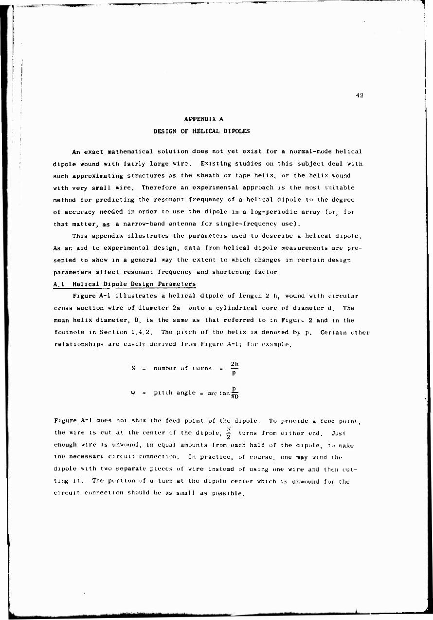
Figure A-l illustrates a helical dipole of lengtn 2 h, wound with circular

cross section wire of diameter 2a onto a cylindrical core of diameter d. The

mean helix diameter, D, is the same as that referred to in Figui<- 2 and in the

footnote in Section 1.4.2. The pitch of the helix is denoted by p. Certain other

relationships are easily derived from Figure A-l; f;>r example,

N - number uf turns = 2h

^ = pitch angle = arc tan =7

Figure A-l does not show the feed point of the dipole. To provide a leod point,

the wire is cut at the center of the dipole, - turns from either end. Just

enough wire is unwound, in equal amounts from each half of the dipole, to make

tne necessary circuit connection. In practice, of course, one may wind the

dipole with two separate pieces of wire instead uf using one wire and then cut-

ting it. The portion of a turn at the dipule center which is unwound for the

circuit connection should be as small as possible.

MM»

■w

1

43

Figure A-l. Parameters ol a helical dipole

■i;.- —

44

A.2 Results and Applications of Dipole Measurements

Thirty-six dipoles were built and their resonant frequencies measured. The p D 2a

parameters ^, — , and — were varied, but the dipole length 2h was held con-

stant at 18 centimeters for all dipoles. Since an 18-centimeter linear dipole

resonates at 833 megacycles, the resonant frequency measured on a given helical

dipole di.ided by 833 equals the value of a for that dipole.

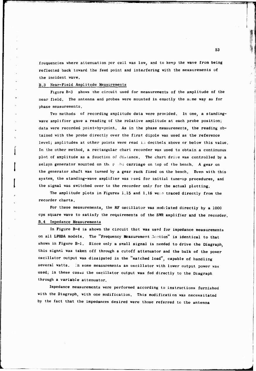
In Figure A-2 are plotted the resonant frequencies and values of s as a func- p

tion of the ratio — for all of the dipoles measured. Each of the three graphs is D

for a different value of —, and the three curves in each graph are for three 2a

different wire iizes (~ ratios).

As an example of a way in which this data can be used, suppose that an an-

tenna designer wants a helical dipole for a given resonant frequency and a given c

value of s. Using, for example, the data in Kandolan and Sichak , he determines

the proper value of pitch to go with his chosen length 2h. He then measures its

resonant frequency. If it is quite close to the desired value, he may be able

to adjust it satisfactorily by shortening or lengthening the dipole slightly.

Then his value of s would be a little different from the intended value. But if

the measured frequency is quite far from the desired value, and he is reluctant to

change 2h and settle for a different s, he can look for a curve in Figure A-2 which 2a D

represents a value of — and —- close to the value he is using, and get from it p *

a new value of — to try.

It was stated in Section 1.1.1 that to a first approximation the wave is as-

sumed to travel along the wire with the velocity of light. This is the same as

saying that s = sir ty. The dashed curve in the first graph of Figure A-2 shows

how rough this approximation is. This curve is a plot of the equation resonant

frequency 1090 sin «|) Mc where the constant 1090 was chosen arbitarily (it 2a o

makes the curve agree with the — = .1135 curve at ^ = 30 ).

Each graph of Figure A-2 shows how resonant frequency changes with wire size,

and the three graphs taken together show how resonant frequency changes with helix

diameter. Figure A-3. however, is designed to give a clearer picture of these 2a

changes. In Figure A-3a, frequency is plotted against wire size (—) for a value

of pitch (—) which gives shortening factors in the neighborhood of 0.5. The range

of wire sizes used here is fairly small; earlier measurements performed on helical

monopoles with a 10-to-l range in wire diameter showed that resonant frequency was

1^mttm*m*^m

T

I

650-

600-

u '550-

O 500

$ «50 i ^ 400-

350

J00 ^

250 1

850-

600-

v 3 550

500

450

^ 400(-

< 350

i so0- 250-

1

650

600-

S 550

fc 500

450

400-

5 350

U 300

250

♦ • TAN'1 P/nO, DEGREE

20 at 30 33 40

—

0/2)i > 0199

^- _L 05

10

10 15 20 2 3 P/0

♦ ■ TAN"1 P/HO. DEGREE

t5 —r-

20 25 30 35 -^

20/0 ■ 12

20/0 ■ 0602

^

30

^-

05

10 -r 15

♦ • TAN" P/HD, DEGREE

^2 S? ^- 20 ^-

_L J_ J_ _L

75

70

«9 «

•O

39 z

3

4» ft O

40 ■

39 •

30

39

" 79

- 70 ^1

65 |

«0 -* m X

- 99 1 - 50 •« - 49 5

? 40

• 39

' 30

05 10 25 30 35

45

19 20 P/D

p 2a Figure A-2. Resonant frequency and shortening factor vs. — and — for three

values of —; 2h = 18 cm = one-half wavelength at 833 Mc

«"—

I i

o Ul

o

500

450

400-

350-

Z 300

K 250

D/2h■ 0199

0/2 h « 0376

0/2h »0552

P/ 0 ■ 1.25

\ 05 10 20

2o/D

25

- 60

-.55

.50

-.45

40

- 35

-.30

(A X o JO H m

o

H O

$

ricur« A-3». tte

frequency and s vs. wire sij igkbarkood of 0.5

— chosen far s In D

650

600

550

500

S *50 ac u.

400

1 3S0

^ 300

250 -

P/0« 3

P/0« 2

P/0» I

2o/D «006

01 02 03 04

D/2h

Figure A-3b. Resonant frequency and s vs. helix di

05 06

2a

75

70 (/) T

65 s H

60 m

55

50

45

40

-35

> O H O 9

y 30

ter for — = 0.06

- - ■ i ntftai i

47

T

proportional to the logarithm of the wire diameter. In Figure A-3b is shown the 2a

effect of helix diameter on resonant frequency for a constant ratio — . Both

of these sets of curves were derived from the curves of Figure A-2. They may be D 2a

summarized by saying that increasing — or decreasing — leads to a smaller

shortening factor

Figure A-3b implies that the presence of dielectric with € > 1 inside r

the helix .nay help in slowinj, the wave propagating along the helix, thus con-

tributing to dipole length reduction. Indeed, the presence of such a dielectric

in a transmission line has just this effect; dielectric loading is often used for 7

this purpose. Li states that the presence of dielectric with € ^1 insiie a r

very thin helix has essentially no effect on the guide wavelength in the helix.

It is doubtful that the helices used in these tests could be called "very thin".

In any case, it is quite possible that the use of a hollow core, which was im-

practical in the laboratory models used here, could reduce the effect of — on ' 2h

resonant frequency.

It is felt that further study could provide much more insight into the effects

of helix parameters and materials on helical dipole performance. In the meantime,

however, experimental techniques will continue to play an important part in the

design of helical antennas.

48

APPENDIX B

MEASUREMENT TECHNIQUES

B.l General

Data of the type presented in this report were obtained through laboratory

measurements of the following four types of quantities: (1) relative phase of

the near field, (2) relative amplitude of the near field, (3) input impedance

referred to the antenna feedpoint, and (4) far-field radiation patterns. In

this appendix are discussed the techniques by which these measurements were per-

formed.

The range of frequencies for which antenna models were constructed and

measured was limited by several factors. A Rohde and Schwarz Diagraph was

used for impedance and phase measurements; its lowest operating frequency is

300 megacycles. The Antenna Laboratory's pattern range facilities give their

most dependable performance at frequencies above 500 Mc (although new facilities

are being obtained for lower-frequency work). The construction of accurately

scaled helical dipoles is difficult for resunant frequencies much above 1000 Mc.

Models of large bandwidth are desirable where "frequency-independent" antennas

are concerned, because only in this way can one get away from end effect and into

a reasonably large frequency region where performance is uniform. In previous work

on log-periodic dipole arrays, two models cf each design had often been built; one

for impedance measurements, characterized by large, good-quality feed cables and a

lower frequency range; the other for pattern measurements, scaled down in size and

up in frequency from the impedance model. This was impractical for the LPHDA

models, for two reasons: the much greater amount of time necessary to build each

model, and the difficulty of scaling individual dipoles accurately with standard

wire sizes. Therefore the impedances and patterns for each set of design parame-

ters were taken on the same model, and a compromise frequency range was used.

For these reasons most of the LPHDA models were built with a lower frequency

limit of 400 ur 420 Mc, and an upper frequency limit of 800 to 1200 Mc. The uni-

formly periodic array used for near-field probing (UPHDA-3) was built with a reso-

nant frequency of about 385 Mc,

B.2 Near-Field Phase Measurements

Relative phase (and amplitude) of the near-field signal on the uniformly peri-

odic array were measured by two different methods of probing. In the first, the

voltage distribution on the antenna feeder was sampled, using a short, straight wire

probe sensitive to the electric field between the two halves of the feeder. This

^rtMMMMMMM

■ ■

49

probe together with a small polystyrene spacer, is visible in Figure 1.14 be-

tween the first and second dipoles. A detailed description of the probe and 3

feeder construction is given in Carrel, pages 184 and 185.

In the second rneihod of probing, the dipole currents were sampled by a

shielded loop which was suspended directly over the feeder and moved up and

down the antenna parallel to the feeder. The loop was oriented in such a way

that the feeder was normal to a plane coi.taining the loop. Thus the loop did

not respond to the feeder current, but only to that component of each dipole

current parallel to the dipole axis. This method gave more consistent and more

easily analyzed results than the first method. Furthermore, agreement of the

k-P diagram with the far-field patterns was better, and data were obtained from

which it was possible to compute far-field patterns.

Although the magnetic field sampled by the probe at any one position is

produced by several nearby dipoles, the principal contribution to the field

close to any one dipole is due to that dipole itself. The readings that were

of the greatest interest, therefore, were those taken when the probe was directly

over each of the dipoles. Readings were taken at intermediate points for the

sake of continuity; the smooth curves connecting all of these points are those

given in Figures 15 and 16. But the principal emphasis in plotting the k-ß

diagram was given only to those points taken at the dipole locations.

Figure B.l shows the phase measurement circuit. The Diagraph is connected

to give readings ol the phase angle of the dipole currents (sampled by the

probe) relative to a reference signal (sampled from the oscillator output by

one of the General Radio Type 874-üA cutoff attenuators). A polar-coordinate

chart was used on the Diagraph .

A detailed description of the measurement procedure is not given here;

after the oscillator was adjusted to the desired frequency and the deflection of

the light spot un the Diagraph peaked with the two pairs of tuning stubs, the

Diagraph was operated in accordance with the instruction nanual furnished with it.

But two features of the circuit should be mentioned. First, since the Diagraph is

reported to work better with a CW than a modulated signal, the modulation necessary

• Since the radial coordinate of the chart (Rohde and Schwarz type 35611/1658) is calibrated in decibels, amplitude readings were occasionally taken by this method also. Those presented in this report, however, were obtained by the method of Section B.3.

^asmmf

\ 50

i

for observing the frequency meter output was imposed only on a small portion of

the oscillator signal, obtained through the first of the two cutoff attenuators.

The required components are shown in the "Frequency Measurement Section" of

Figure B-l. Secondly, a new plexiglass screen was substituted for the original

one on the Diagraph. On this new screen, the polar coordinate chart was fastened

with one pin in the center, instead of two pins at the edge as in the original

screen. This center pin featured a spring-loaded arrangement which caused the

chart to turn normally with the screen, but allowed it to be rotated with respect

to the screen whenever necessary. Since it was desired to establish the phase

of the current in the first dipole as phase reference or "zero-phase", the Dia-

graph phase indicator was first peaked with the probe over the first dipole; then

the chart rotated, while the screen was held fixed, until the zero-degree line

of the chart fell over the light spot. By this means it was also possible to com-

pensate for changes in the phase shift of the signal through the variable attenu-

ator whenever the attenuator setting was changed. Such changes were often neces-

sary to keep the light spot in view on the chart.

Figure B-2 is a photograph of the bench used for phase measurements (and

also for amplitude and impedance measurements). The antenna mounted on the right-

hand end of the bench is UPHDA-3, The loop probe is not shown; the probe connec-

ted to the equipment in this photograph is the voltage probe mentioned earlier in

this section. When measurements were being taken, the bench was rolled up to an

anechoic chamber so that the antenna extended into the chamber. The perforated

aluminum screen shielded the equipment from stray radiation.

When the probe is moved along the antenna, the coaxial cable connected to it

must bend. This flexing introduces some degree of change in phase shift through 4

the cable, depending on the type of cable and how sharply it is bent. To keep

this flexing (and its effect on measured data) to a miniumum, the excess cable is

taken up on the large wheei, shown above the left-hand end of the bench. The signal

is fed through a rotary Joint in the hub of the wheel. A test showed that the phase

shift of a »ignal through the cable when completely wound on the wheel was so close to

the phase shift when the cable was unwound that the difference was almost unmeasurable.

One important feature of this apparatus, not shown in the photograph, must

be mentioned. Whenever phase or amplitude measurements were being made, a portion

of the antenna next to the screen and including the last three dipoles was en-

closed in a large block of microwave absorber. The purpose of this material was

to absorb the wave pijpagating along the antenna from the feed point, at those

51

5 u s a a

I ID

-i f- > • 1 o» • 1 ^ c

1! > 1 V

i 1 u

o Ul a.

i s -i I w -1 o 1 3 5 o 1 0

a> 0» 1 w

o 1 K 1 ^

o u

I CQ

3

wmm

52

Figure B-2. Laboratory equipment connected for phase measurements

^^t^»^^_ . .. MOM^H^

■ B^y

53

frequencies where attenuation per ceil was low, and to keep the wave from being

reflected back toward the feed point and interfering with the measurements of

the incident wave.

B.3 Near-Field Amplitude Measurements

Figure B-3 shows the circuit used for measurements of the amplitude of the

near field. The antenna and probes were mounted in exactly the si.;me way as for

phase measurements.

Two methods of recording amplitude data were provided. In one, a standing-

wave amplifier gave a reading of the relative amplitude at each probe position;

data were recorded point-by-point. As in the phase measurements, the reading ob-

tained with the probe directly over the first dipole was used as the reference

level; amplitudes at other points were read 1.1 decibels above or below this value.

In the other method, a rectangular chart recorder was used to obtain a continuous

plot of amplitude as a function of dit. Lance, The chart drive was controlled by a

selsyn generator mounted on thi p hj carriage on top of the bench, A gear on

the generator shaft was turned by a gear rack fixed on the bench. Even with this

system, the standing-wave amplifier was vsed for initial tune-up procedures, and

the signal was switched over to the recorder only for the actual plotting.

The amplitude plots in Figures 1,15 and 1,16 weia traced directly from the

recorder charts.

For these measurements, the RF oscillator was modi lated directly by a 1000

cps square wave to satisfy the requirements of the SWR amplifier and the recorder.

B.4 Impedance Measurements

In Figure B-4 is shown the circuit that was used for impedance measurements

on all LPHDA models. The "Frequency Measurement .lection" is identical to that

shown in Figure B-l. Since only a small signal is needed to drive the Diagraph

this signp.i was taken off through a cutoff attenuator and the bulk of the power

oscillator output was dissipated in the "matched load", capable of handling

several watts. In some measurements an oscillator with lower output power was

used; in these cases the oscillator output was fed directly to the Diagraph

through a variable attenuator.

Impedance measurements were performed according to instructions furnished

with the Diagraph, with one modification. This modification was necessitated

by the fact that the impedances desired were those referred to the antenna

mmi •■■■:'•"—"— —i 1—

54

Hi

UJ S o -I o CD

K W

oc u. ^ 3 M a.

s <

CO •1

OC u

1 o -1 u J Q. o o M o O (0

c 01 E (U i_ 3

s 0) s 0) •o 3

a E 3)

o

a in ■H 3 "O «-»

y «4 o a PH a CQ cd

n i

CQ

(U u 3 (ID

■H

m^^m t^*mi

——

^

bl

55

O w z

2E o

A/SAA

c bl Z u Ui c (0

bl

s OT

»- z f» ÜJ < S bl bl a oc 3 (0 < bl S

I bl 0) < Z

c ! o >•

b V

o U bl z M bl 3 o bl K b.

M

i

e

v 3

i c (4

0

5 (S «1 •H 3 ■O *•

id X u u « o a

•H a CO A

I 00

2

(X

^J

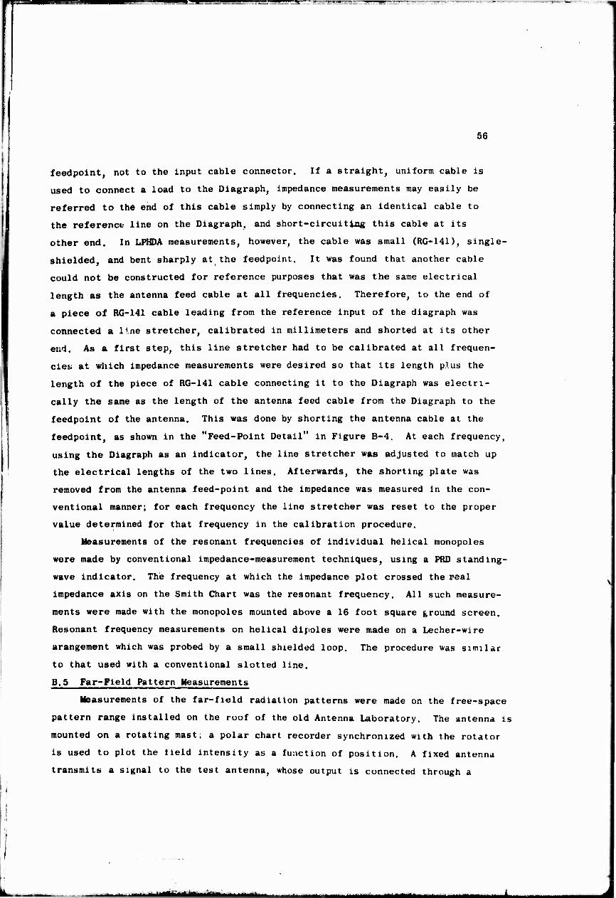
BBM^gTB^ll^^M^P^^gM^^^——■—y^wy^^^^^^^^^*^" "T'T.. "m^ ^ :v""' '■**■'■■''''*, , "g^TgyT.'.'!1,? . L, .f "?!i" .Ty^"-' ■, ' ■ ■ '■ "^^ "■■^^■■^y ^J .MI'-I .^WMJI ■

56

feedpoint, not to the input cable connector. If a straight, uniform cable is

used to connect a load to the Diagraph, impedance measurements may easily be

referred to th6 end of this cable simply by connecting an identical cable to

the reference line on the Diagraph, and short-circuiting this cable at its

other end. In LPHDA measurements, however, the cable was small (RG-141), single-

shielded, and bent sharply at the feedpoint. It was found that another cable

could not be constructed for reference purposes that was the same electrical

length as the antenna feed cable at all frequencies. Therefore, to the end of

a piece of RG-141 cable leading from the reference input of the diagraph was

connected a line stretcher, calibrated in millimeters and shorted at its other

end. As a first step, this line stretcher had to be calibrated at all frequen-

cies; at which impedance measurements were desired so that its length plus the

length of the piece of RG-141 cable connecting it to the Diagraph was electri-

cally the same as the length of the antenna feed cable from the Diagraph to the

feedpoint of the antenna. This was done by shorting the antenna cable at the

feedpoint, as shown in the "Feed-Point Detail" in Figure B-4. At each frequency,

using the Diagraph as an indicator, the line stretcher was adjusted to match up

the electrical lengths of the two lines. Afterwards, the shorting plate was

removed from the antenna feed-point and the impedance was measured in the con-

ventional manner; for each frequency the line stretcher was reset to the proper

value determined for that frequency in the calibration procedure.

Measurements of the resonant frequencies of individual helical monopoles

were made by conventional impedance-measurement techniques, using a PRD standing-

wave indicator. The frequency at which the impedance plot crossed the peal

impedance axis on the Smith Chart was the resonant frequency. All such measure-

ments were made with the monopoles mounted above a 16 foot square ground screen.

Resonant frequency measurements on helical dipoles were made on a Lecher-wire

arangement which was probed by a small shielded loop. The procedure was similar

to that used with a conventional slotted line.

B.5 Far-Field Pattern Measurements

Measurements of the far-field radiation patterns were made on the free-space

pattern range installed on the roof of the old Antenna Laboratory. The antenna is

mounted on a rotating mast; a polar chart recorder synchronized with the rotator

is used to plot the field intensity as a function of position. A fixed antenna

transmits a signal to the test antenna, whose output is connected through a

— i ii JMt^^tl

W ' '" m

57

bolometer (or crystal, if the signal Is weak) to an amplifier which drives the re-

corder pen In a radial direction over the chart. The resulting plots are propor-

tional to field intensity; their radial coordinates must be squared to give the

power pattern. Half-power beamwidths, therefore, are obtained by measuring the

angle within which the measured field Intensity is equal to or greater than 0.707

times the peak intensity.

' ■> • -V ■ "T— --TTJ-"

UNCLASSIFIED Si'iiintv C Lissifuatiim

DOCUMENT CONTROL DATA -R&D Svt'ufltV I 7«J»M/H Htlitn iif litte, htuh "t .ih-fr.u t ttifl ttnh-xiti,' .imutt.iti, ■[) rnu ■( In- entt'tfd altffi tin- ,IVI r.ill rtfuirl J . . l.t^wttieiU

'AlitelnhäNLaV6ral6lr^7''1ÖepaHment of Electrical Engineering, Engineering Experiment Station,

University of Illinois, Urbana, Illinois

;a. Rf roH i •'. ( r LJ i* i t > »" L A SI ■ JC A r lOfj

UNCLASSIFIED th. Gwour

1 REPORT TITLE

BROADBAND ARRAYS OF HELICAL DIPOLES

4 DESCRIPTIVE HOtEi (Ti'pe ol trport and inctwivv üalv*)

Part 2 of Final Report, 1 June 1962-31 August 1963 5 AU THORtsi ('Firs/name, middle initial, last name)

D. T. Stephenson and P. E. Mayes

6 REPORT DATE

January 1964 7«. TOTAL NO. OK PAGES

57 rb. NO OF REPS

11 B«. CONTRACT OR GRANT NO

NEL 30508A b. PROJEC T NO

9«. ORIGINATOR'S REPOHT NUMBERtSI

Technical Report 2

9K OTHER REPORT NOISI (Any ulher numbers thai muy he osslgncil this report)

10 DISTRIBUTION STAT EMENT

Distribution of this document is unlimited.

11 SUPPLEMENTARY NOTES 12 SPONSORING MILI T AR Y ACTIVITY

Navy Electronics Laboratory San Diego, California 92152

11 ABSTRACT

Thts report deals with the problem of reducing the resonant length of radiating elements of log-periodic dipole antenna arrays by the use of helical dipole elements. Some consideration is given also to the problem of boom length shortening Reduced size log-periodic arrays are required to make practical shipborne applica- tions in the high frequency band at frequencies as low as 8 MHz. Several reduced scale models were built using helical dipole elements and compared with similar designs using linear dipole elements. Directive gains and impedance characteristics were compared. An element shortening factor of 0. 54 was used. Some mixed dipole arrays, where only the longer low frequency elements were shortened, also were tested.

Conclusions are that helical dipoles are useful and practical size-reduced elements for log-periodic arrays. However, boom length is increased by dipole length shortening and antenna performance somewhat impaired. The most practical design is a log-periodic mixed dipole array. Measurement techniques are treated in an appendix.

DDiFOoRM473 S '. 0 '01 ■ 807. o8'J 1

(PAi-l 1 ) UNCLASSIFIED StMijntv Cl**ssifu dlion

——i im*m*

UNCLASSIFIED Security Classification

KEY WORDS

RO L C W T

Antenna Arrays

Helical Antennas

Log Periodic Antennas

DD;r..1473 BACK, (PAGE 2!

UNCLASSIFIED Srcurity Classification