1

Antarctic Sea Ice Variability and Trends, 1979-2010

C. L. Parkinson and D. J. Cavalieri

Cryospheric Sciences Laboratory/Code 615

NASA Goddard Space Flight Center

Greenbelt, MD 20771, USA

Corresponding Author: Claire Parkinson, phone 301-614-5715, fax 301-614-5644, email

address Claire.L.Parkinson@nasa.gov.

For submission to The Cryosphere,

February 2012

https://ntrs.nasa.gov/search.jsp?R=20120009528 2019-02-15T06:39:44+00:00Z

2

Abstract. In sharp contrast to the decreasing sea ice coverage of the Arctic, in the

Antarctic the sea ice cover has, on average, expanded since the late 1970s. More

specifically, satellite passive-microwave data for the period November 1978 – December

2010 reveal an overall positive trend in ice extents of 17,100 ± 2,300 km2/yr. Much of the

increase, at 13,700 ± 1,500 km2/yr, has occurred in the region of the Ross Sea, with lesser

contributions from the Weddell Sea and Indian Ocean. One region, that of the

Bellingshausen/Amundsen Seas, has, like the Arctic, instead experienced significant sea

ice decreases, with an overall ice extent trend of -8,200 ± 1,200 km2/yr. When examined

through the annual cycle over the 32-year period 1979-2010, the Southern Hemisphere sea

ice cover as a whole experienced positive ice extent trends in every month, ranging in

magnitude from a low of 9,100 ± 6,300 km2/yr in February to a high of 24,700 ± 10,000

km2/yr in May. The Ross Sea and Indian Ocean also had positive trends in each month,

while the Bellingshausen/Amundsen Seas had negative trends in each month, and the

Weddell Sea and Western Pacific Ocean had a mixture of positive and negative trends.

Comparing ice-area results to ice-extent results, in each case the ice-area trend has the

same sign as the ice-extent trend, but differences in the magnitudes of the two trends

identify regions with overall increasing ice concentrations and others with overall

decreasing ice concentrations. The strong pattern of decreasing ice coverage in the

Bellingshausen/Amundsen Seas region and increasing ice coverage in the Ross Sea region

is suggestive of changes in atmospheric circulation. This is a key topic for future research.

3

1 Introduction

Sea ice spreads over millions of square kilometers of the Southern Ocean at all times

of the year and over an area larger than the Antarctic continent in the midst of the austral

winter, with February typically the month of minimum ice coverage and September

typically the month of maximum ice coverage (Fig. 1). The ice hinders exchanges between

the ocean and atmosphere, reflects solar radiation back to space, is an obstacle to ship

travel, and has numerous impacts on plant and animal species in the Southern Ocean (e.g.,

Ainley et al., 2003; Parkinson, 2004). As an integral component of the climate system, the

sea ice cover both affects and reflects changes in other climate components, hence making

it of particular interest that the Antarctic sea ice cover has not experienced the prominent

decreases witnessed over recent decades in the Arctic sea ice cover (Parkinson and

Cavalieri, 2008; Cavalieri and Parkinson, 2008).

Unfortunately, the record of sea ice is quite incomplete for any time prior to the

1970s, due in large part to its remoteness, the harsh conditions of the polar environment,

and the lack of convenient means for remotely sensing the ice at that time. In great

contrast, since the late 1970s, the distribution of polar sea ice is one of the best recorded of

all climate variables. The reason is the ease of distinguishing sea ice from liquid water in

satellite passive-microwave observations (e.g., Zwally et al., 1983) and the near-

continuous presence of at least one operating satellite passive-microwave instrument over

almost the entire period since October 1978.

Through satellite passive-microwave observations, there now exists a solid record of

the distribution and extent of Arctic and Antarctic sea ice coverage and their changes since

the late 1970s. This record has allowed persuasive quantification of an overall decreasing

4

Arctic sea ice coverage (e.g., Parkinson et al., 1999; Meier et al., 2007), as expected in

light of Arctic warming (ACIA, 2005), and, at a markedly lesser rate, a less expected

increasing Antarctic sea ice coverage (e.g., Stammerjohn and Smith, 1997; Zwally et al.,

2002). In 2008, these trends were detailed regionally and hemispherically for the period

November 1978 through December 2006 by Parkinson and Cavalieri (2008) for the Arctic

and by Cavalieri and Parkinson (2008) for the Antarctic. With four additional years of data

analyzed, we are now updating those results through 2010, doing so for the Antarctic in

this paper and for the Arctic in a companion paper (Cavalieri and Parkinson, 2012).

2 Data

This study is based on satellite passive-microwave data from the Scanning

Multichannel Microwave Radiometer (SMMR) on NASA’s Nimbus 7 satellite, the Special

Sensor Microwave Imager (SSMI) on the F8, F11, and F13 satellites of the Department of

Defense’s Defense Meteorological Satellite Program (DMSP), and the Special Sensor

Microwave Imager Sounder (SSMIS) on the DMSP F17 satellite. Nimbus 7 was launched

in late October 1978, and the SMMR instrument obtained data every other day for most of

the period from 26 October 1978 through 20 August 1987. The first SSMI was launched

on the DMSP F8 satellite in June 1987, and the sequence of F8, F11, and F13 SSMIs

collected data on a daily basis for most of the period from 9 July 1987 to the end of 2007,

after which the F13 SSMI began to degrade. The F17 SSMIS was the second SSMIS in

orbit and was launched in November 2006, with a daily data record beginning in mid-

December 2006. In this paper, we use SMMR data for the period November 1978 – July

1987, SSMI data for August 1987 – December 2007, and SSMIS data for January 2008 –

5

December 2010. These data are archived at and available from the National Snow and Ice

Data Center (NSIDC) in Boulder, Colorado.

The SMMR, SSMI, and SSMIS data are used to calculate ice concentrations (percent

areal coverages of ice) with the NASA Team algorithm (Gloersen et al. 1992; Cavalieri et

al., 1995), and the ice concentrations are mapped at a grid cell size of 25 km x 25 km.

These ice concentrations are then used to calculate sea ice extents (summed areas of all

grid cells in the region of interest having at least 15% sea ice concentration) and sea ice

areas (summed products of the grid cell areas times the ice concentrations for all grid cells

in the region of interest having at least 15% sea ice concentration). Details on the merging

of the SMMR, F8, F11, and F13 records can be found in Cavalieri et al. (1999), and details

on the merging of the F13 and F17 records, taking advantage of the full year of data

overlap in 2007, can be found in Cavalieri et al. (2012). Explanation for the 15% threshold

can be found in Parkinson and Cavalieri (2008).

Ice extents and ice areas were averaged for each day of available data, with missing

data filled in by spatial and temporal interpolation, and these daily averages were

combined to monthly, seasonal, and yearly averages. To obtain long-term trends for the

monthly results, the seasonal cycle was removed by creating monthly deviations, which

were calculated by subtracting from each individual monthly average the 32-year average

for that month (or, in the case of November and December, the 33-year average). This

follows the procedure in Parkinson et al. (1999) and subsequent works.

Lines of linear least squares fit were calculated for the monthly deviation data and

for the yearly, seasonal, and monthly averages. Standard deviations of the slopes of these

lines were calculated based on Taylor (1997), and a rough indication of whether the trends

6

are statistically significant as non-0 was determined by calculating the ratio R of the trend

to its standard deviation, identifying a trend as significant at a 95% confidence level if R

exceeds 2.04 and significant at a 99% confidence level if R exceeds 2.75. This is

essentially using a two-tailed t-test with 30 degrees of freedom (2 less than the number of

years). It gives a useful suggestion of the relative significance of the slopes, although, like

other tests of statistical significance, is imperfect in its application to the real world (e.g.,

Santer et al., 2000).

As in Cavalieri and Parkinson (2008) and earlier studies, results are presented for the

following five regions of the Southern Ocean: Weddell Sea (60°W - 20°E, plus the small

ocean area between the east coast of the Antarctic Peninsula and 60°W), Indian Ocean

(20°E - 90°E), Western Pacific Ocean (90°E - 160°E), Ross Sea (160°E - 130°W), and the

combined Bellingshausen and Amundsen Seas (130°W - 60°W) (Fig. 2).

3 Results

3.1 Sea ice extents

3.1.1 Southern hemisphere total

Figure 3 presents plots of Southern Hemisphere monthly average sea ice extents and

monthly deviations for the period November 1978 – December 2010 and yearly and

seasonal averages for 1979-2010. On average over the 32-year period, the ice extents

ranged from a minimum of 3.1 x 106 km2 in February to a maximum of 18.5 x 106 km2 in

September (Fig. 3a inset).

In view of the large seasonal cycle, the plot of monthly averages is dominated by this

cycle (Fig. 3a). However, when the seasonal cycle is removed, in the monthly deviations,

7

the existence of an upward trend becomes clear, with a positive slope of 17,100 ± 2,300

km2/yr, statistically significant at the 99% confidence level, for the period November 1978

– December 2010 (Fig. 3b). This slope has increased from the 11,100 ± 2,600 km2/yr trend

reported by Cavalieri and Parkinson (2008) for the monthly deviations for the shorter

period November 1978 – December 2006, and indeed the highest deviations in the 32-year

record are within the newly added last 4 years of the data set (Fig. 3b).

The slopes of the lines of linear least squares fit through the yearly and seasonal ice

extent values plotted in Fig. 3c, for the Southern Hemisphere total, are presented in Table

1, as are the corresponding slopes for each of the five analysis regions. For the yearly

averages, the Southern Hemisphere slope is 17,500 ± 4,100 km2/yr (1.5 ± 0.4 %/decade)

(Table 1), increased from a slope of 11,500 ± 4,600 km2/yr for the shorter period ending in

December 2006 (Cavalieri and Parkinson, 2008) and within 3% of the slope for the

monthly deviations, which have a somewhat smaller slope in part because of including at

the start of the record the initial months of November and December 1978, both of which

have ice extent values above the line of least squares fit (Fig. 3b). The much higher

standard deviation for the slope of the yearly averages versus the monthly deviations

reflects the far smaller number of data points (32 years versus 386 months).

Seasonally, the slopes for all four seasons are positive, with the largest slope being

for autumn, at 23,500 ± 8,900 km2/yr, and the smallest slope being for summer, at 13,800 ±

7,700 km2/yr (Table 1). For every season, the slopes have increased with the addition of

the 2007-2010 data (Table 1 versus Cavalieri and Parkinson, 2008). On a percent per

decade basis, the largest seasonal slope is for summer, at 3.6 ± 2.0 %/decade (Table 1).

8

3.1.2 Regional Results

Figure 4 presents monthly deviation plots for each of the five Antarctic sea ice

regions, as well as for the total. For this five-part sectorization, the Western Pacific Ocean

shows no significant trend, the Weddell Sea, Indian Ocean, and Ross Sea all have positive

trends, and the Bellingshausen/Amundsen Seas region has a negative trend, with the

highest magnitude trend being the 13,700 ± 1,500 km2/yr positive trend for the Ross Sea

and the second highest magnitude trend being the -8,200 ± 1,200 km2/yr negative trend for

the Bellingshausen/Amundsen Seas (Fig. 4). The trends for the Ross Sea,

Bellingshausen/Amundsen Seas, and Indian Ocean are all statistically significant at the

99% confidence level, while the trend for the Weddell Sea is statistically significant at the

95% confidence level.

The Ross Sea has positive trends in each season, with its highest seasonal trend being

in spring, at 17,600 ± 5,100 km2/yr, and its lowest seasonal trend being in summer, at

10,000 ± 4,800 km2/yr (Table 1). In the opposite direction, the Bellingshausen/Amundsen

Seas region has negative trends in each season, ranging in magnitude from -2,600 ± 4,100

km2/yr in winter to -14,300 ± 2,600 km2/yr in summer (Table 1). Like the Ross Sea, the

Indian Ocean has positive ice extent trends in each season, although the magnitudes are

consistently lower than those in the Ross Sea, both on a km2/yr basis and on a %/decade

basis. The Weddell Sea and Western Pacific Ocean both have small, statistically

insignificant negative trends in winter and spring and higher magnitude positive trends in

summer and autumn, with positive but statistically insignificant trends for the yearly

averages (Table 1).

9

On a monthly basis, the Ross Sea has positive trends of at least 7,000 km2/yr in each

month, and the Indian Ocean has positive trends in each month, although consistently of

lesser magnitude than those in the Ross Sea (Fig. 5). The Bellingshausen/Amundsen Seas

region has negative trends in each month, although much more so in summer than in

winter; and the Weddell Sea has positive trends for each month January – June and a

mixture of positive and negative trends for the rest of the year, with near-0 values in July,

August, and September. The Western Pacific Ocean has positive trends in the first half of

the year and predominantly negative trends in the second half, although with no trend of

magnitude as high as 5,000 km2/yr (Fig. 5). The net result is a Southern Hemisphere sea

ice cover with positive 32-year sea ice extent trends in every month of the year, ranging in

magnitude from a low of 9,100 ± 6,300 km2/yr in February to a high of 24,700 ± 10,000

km2/yr in May (Fig. 5).

3.2 Sea Ice Areas

3.2.1 Southern Hemisphere Total

Figures 6-8 and Table 2 present for sea ice areas the corresponding information to

what is presented in Figs. 3-5 and Table 1 for ice extents. In all instances, ice areas are

necessarily lower than or equal to ice extents, with equality only coming in cases of no ice

cover or complete, 100% ice coverage.

The hemispheric ice area monthly averages (Fig. 6a) show the same basic seasonal

cycle as the ice extent monthly averages (Fig. 3a), although with lower values. For the ice

areas, the 32-year average seasonal cycle has values ranging from 2.0 x 106 km2 in

February to 14.6 x 106 km2 in September (Fig. 6a inset). The ice area monthly deviation

10

plot has some noticeable differences from the ice extent monthly deviation plot, and the

slope of the ice area trend line is somewhat lower than that for the ice extents, being

14,900 ± 2,100 km2/yr (Fig. 6b versus Fig. 3b), suggesting a trend toward lessened overall

ice concentration. As is the case for ice extents, the last 4 years of the data set contain

within them the highest monthly deviations of the entire data set, with the result that the

trend has increased over the 9,600 ± 2,400 km2/yr trend reported in Cavalieri and

Parkinson (2008) for November 1978 – December 2006.

As with the ice extents, the sea ice area trends for the Southern Hemisphere are

positive in each season and for the yearly average, with the highest magnitude ice area

seasonal trend being for autumn, at 25,800 ± 8,300 km2/yr (Table 2). The lowest

magnitude seasonal trend for ice areas, however, is for spring rather than for summer

(Table 2). Furthermore, for summer, winter, and spring, the ice area trend has lower

magnitude than the ice extent trend, whereas for autumn the ice area trend has higher

magnitude than the ice extent trend (Tables 1 and 2). This suggests that in summer, winter,

and spring the ice cover became less compact whereas in autumn it became more compact,

overall for the 1979-2010 period. On a %/decade basis, the greatest seasonal ice area slope

is for summer, at 4.6 ± 2.4 %/decade (Table 2).

3.2.2 Regional Results

Regionally, the basic qualitative results remain largely the same for ice areas as for

ice extents. Specifically, the 32-year ice area monthly deviation trends are positive for the

Weddell Sea, Indian Ocean, and Ross Sea, and are negative for the

Bellingshausen/Amundsen Seas, with the highest magnitude slope being the positive slope

11

for the Ross Sea and the second highest magnitude slope being the negative slope for the

Bellingshausen/Amundsen Seas (Fig. 7). One difference is that the positive slope for the

ice area monthly deviations for the Western Pacific Ocean is statistically significant at the

95% level, versus the statistically insignificant positive slope for the ice extent monthly

deviations. The Western Pacific Ocean, which has by far the lowest of the six slopes in

both the ice area and ice extent cases, is the only one of the five regions that has a higher

slope for the ice area monthly deviations than for the ice extent monthly deviations (Figs. 4

and 7).

Monthly trends for ice areas (Fig. 8) also show many similarities with the monthly

trends for ice extents (Fig. 5), including positive trends for every month for the Indian

Ocean and Ross Sea and negative trends (some near 0) for every month for the

Bellingshausen/Amundsen Seas. The magnitudes differ, however, with generally lower

magnitude ice area slopes (versus ice extent slopes) in the Ross Sea, Indian Ocean, and

Bellingshausen/Amundsen Seas, suggesting a lessening of the ice compactness in the Ross

Sea and Indian Ocean cases, with positive ice area and ice extent slopes, but an increase of

the ice compactness in the Bellingshausen/Amundsen Seas, with negative ice area and ice

extent slopes (Figs. 5 and 8). The Weddell Sea and Western Pacific Ocean have a more

mixed pattern, both in the sign of the slope and in how the ice area and ice extent slopes

differ (Figs. 5 and 8).

4 Discussion

The upward trends in sea ice extents and areas reported here for the Southern

Hemisphere are in sharp contrast to the situation in the Arctic, where downward trends

12

have been reported since the late 1980s (Parkinson and Cavalieri, 1989) and have become

stronger over time (Johannessen et al., 1995; Parkinson et al., 1999; Meier et al., 2007;

Comiso et al., 2008; Cavalieri and Parkinson, 2012). The sea ice decreases in the Arctic are

readily tied to the warming that has also been reported in the Arctic and to the broader

phenomenon of global warming (e.g., ACIA, 2005).

In the Antarctic case, the sea ice decreases in the region of the

Bellingshausen/Amundsen Seas can also be tied to warming, as they have occurred in

conjunction with marked warming in the Antarctic Peninsula/Bellingshausen Sea vicinity

(Vaughn et al., 2003). The sea ice increases around much of the rest of the continent might

similarly be aligned with overall cooling in those regions (e.g., Vaughn et al., 2003),

although this is less certain, as there is considerable uncertainty about temperature trends in

much of the Antarctic outside of the well-documented Peninsula region, with recent

reconstructions questioning earlier results (O’Donnell et al., 2011).

Antarctic sea ice variability since the late 1970s is well-documented (e.g., Gloersen

et al., 1992; Zwally et al., 2002; Cavalieri and Parkinson, 2008) and has been examined in

connection with other Earth-system phenomena, such as the El Niño-Southern Oscillation

(ENSO) (e.g., Simmonds and Jacka, 1995; Watkins and Simmonds, 2000; Rind et al.,

2001; Kwok and Comiso, 2002; Yuan, 2004; Stammerjohn et al., 2008) and the Southern

Annual Mode (SAM) (e.g., Hall and Visbeck, 2002; Thompson and Solomon 2002; Goose

et al., 2008; Stammerjohn et al., 2008; Comiso et al., 2011). Rind et al. (2001) suggest less

sea ice in the Pacific and more sea ice in the Weddell Sea in an El Niño year, and vice

versa in a La Niña year.

13

Of particular interest are the studies that address the observed pattern of negative sea

ice trends in the Bellingshausen Sea and positive sea ice trends in the Ross Sea (Figs. 4 and

7). For instance, Stammerjohn et al. (2008) find that, at least over the period of their study,

1979-2004, this pattern appears associated with decadal changes in the mean state of the

SAM and the response of the sea ice cover to the ENSO, with the response being

particularly strong when an El Niño occurred with a negative SAM index and when a La

Niña occurred with a positive SAM index. However, intriguing as these correspondences

might be, their likely importance is weakened by the fact that the connections between sea

ice and the ENSO and SAM are “not as consistent over time” in the other regions of the

Antarctic sea ice cover (Stammerjohn et al., 2008).

Thompson and Solomon (2002) explain the warming of the Antarctic Peninsula

region and the apparent cooling of much of the rest of Antarctica by connection with a

trend toward a strengthened circumpolar flow in the summer and fall, with the tropospheric

trends traced to trends in the polar vortex of the lower stratosphere. As these latter trends

are largely due to Antarctic ozone depletion, the pattern of sea ice changes thereby

becomes tied to human-caused stratospheric ozone depletion (Thompson and Solomon,

2002). Shindell and Schmidt (2004) also connect the cooling over much of Antarctica to

ozone changes and the SAM, but they do not explicitly further connect these changes to

the pattern of sea ice changes.

In a paper focused on the contrast between the sea ice decreases in the

Bellingshausen/Amundsen Seas and increases in the Ross Sea (as in Figs. 4 and 7), Turner

et al. (2009) also, like Thompson and Solomon (2002), tie this pattern to stratospheric

ozone depletion. In the Turner et al. paper, a key mechanism is increased cyclonic

14

atmospheric flow over the Amundsen Sea, bringing warm air from the north over the

Bellingshausen Sea and cold air from the south over the Ross Sea. Increased cyclonic flow

would indeed thereby provide a persuasive explanation of the pattern of sea ice changes.

Connecting the increased cyclonic flow to the human-caused ozone depletion is model-

based and less certain; and the paper concludes that “the observed sea ice increase might

still be within the range of natural climate variability” (Turner et al., 2009).

In a modeling study specifically addressing the issue of whether the ozone hole has

contributed to increased Antarctic sea ice extent, Sigmond and Fyfe (2010) conclude that it

has not. In fact, their climate model simulates that stratospheric ozone depletion would

lead to a decrease in Antarctic sea ice, and hence they conclude that the observed increase

in Antarctic sea ice extent must be caused by something other than ozone depletion.

All in all, the varied results of studies attempting to explain the sea ice changes in the

Antarctic are intriguing but not conclusive. It remains the case that the increases in sea ice

coverage in the Antarctic (Figs. 3-8) are less readily tied to global warming than are the

decreases in the Arctic ice coverage. Nonetheless, both ice covers are part of the climate

system, and the overall changes (Figs. 3 and 6) and patterns of change (Figs. 4, 5, 7, and 8)

in the Antarctic ice cover are components of the pattern of global changes, just as the

Arctic changes are. Hence, even though the Antarctic changes are not yet completely

understood, eventually their connections with the rest of the global system (atmosphere,

oceans, land, ice, and biosphere) should be explained, as future studies reveal more of the

details of the ongoing changes in the Earth system.

15

Acknowledgments. The authors thank Nick DiGirolamo of Science Systems and

Applications Incorporated (SSAI) and Al Ivanoff of ADNET Systems for considerable

help in processing the data and Nick DiGirolamo additionally for help in generating the

figures. We also thank the National Snow and Ice Data Center (NSIDC) for providing the

DMSP SSMI and SSMIS daily gridded brightness temperatures. This work was supported

with much-appreciated funding from NASA’s Cryospheric Sciences Program.

16

References

ACIA, Arctic Climate Impact Assessment. Cambridge, UK: Cambridge University

Press, 1,042 pp., 2005.

Ainley, D. G., Tynan, C. T., and Stirling, I.: Sea ice: A critical habitat for polar

marine mammals and birds, in Sea Ice: An introduction to Its Physics, Chemistry, Biology,

and Geology, ed. by D. N. Thomas and G. S. Dieckmann. Oxford: Blackwell Science, pp.

240-266, 2003.

Cavalieri, D. J. and Parkinson, C. L.: Antarctic sea ice variability and trends, 1979-

2006, J. Geophys. Res., 113, C07004, doi:10.1029/2007JC004564, 2008.

Cavalieri D. J. and Parkinson, C. L.: Arctic sea ice variability and trends, 1979-2010,

submitted to The Cryosphere, 2012.

Cavalieri, D. J., St. Germain, K., and Swift, C. T.: Reduction of weather effects in

the calculation of sea ice concentration with the DMSP SSM/I, J. Glaciol., 44, 455-464,

1995.

Cavalieri, D. J., Parkinson, C. L., Gloersen, P., Comiso, J. C., and Zwally, H. J.:

Deriving long-term time series of sea ice cover from satellite passive-microwave

multisensor data sets, J. Geophys. Res., 104, C7, 15,803-15,814, 1999.

Cavalieri, D. J., Parkinson, C. L., DiGirolamo, N., and Ivanoff, A.: Intersensor

calibration between F13 SSMI and F17 SSMIS for global sea ice data records, IEEE

Geosci. Remote Sensing Lett., 9, 2, 233-236, 2012.

Comiso, J. C., Parkinson, C. L., Gersten, R., and Stock, L.: Accelerated decline in

the Arctic sea ice cover, Geophys. Res. Lett., 35, L01703, doi:10.1029/2007GL031972,

2008.

17

Comiso, J. C., Kwok, R., Martin, S., and Gordon, A. L.: Variability and trends in sea

ice extent and ice production in the Ross Sea, J. Geophys. Res., 116, C04021, doi:

10.1029/2010JC006391, 2011.

Gloersen, P., Campbell, W. J., Cavalieri, D. J., Comiso, J. C., Parkinson, C. L., and

Zwally, H. J.: Arctic and Antarctic Sea Ice, 1978-1987: Satellite Passive-Microwave

Observations and Analysis. Washington, D.C.: National Aeronautics and Space

Administration, 290 pp., 1992.

Goosse, H., Lefebvre, W., de Montety, A., Crespin, E., and Orsi, A. H.: Consistent

past half-century trends in the atmosphere, the sea ice and the ocean at high southern

latitudes, Climate Dynamics, 33, no. 7-8, 999-1016, doi:10.1007/s00382-008-0500-9,

2008.

Hall, A. and Visbeck, M.: Synchronous variability in the Southern Hemisphere

atmosphere, sea ice, and ocean resulting from the Annular Mode, J. Climate, 15, 3043-

3057, 2002.

Johannessen, O. M., Miles, M., and Bjørgo, E.: The Arctic’s shrinking sea ice,

Nature, 376, 126-127, doi:10.1038/376126a0, 1995.

Kwok, R., and Comiso, J. C.: Southern Ocean climate and sea ice anomalies

associated with the Southern Oscillation, J. Climate, 15, 487-501, 2002.

Meier, W. N., Stroeve, J., and Fetterer, F.: Whither Arctic sea ice? A clear signal of

decline regionally, seasonally and extending beyond the satellite record, Ann. Glaciology,

46, 428-434, 2007.

18

O’Donnell, R., Lewis, N., McIntyre, S., and Condon, J.: Improved methods for PCA-

based reconstruction: Case study using the Steig et al. (2009) Antarctic temperature

reconstructions, J. Climate, 24, 2099-2115, 2011.

Parkinson, C. L.: Southern Ocean sea ice and its wider linkages: Insights revealed

from models and observations, Antarctic Science, 16, 4, 387-400, doi:

10.1017/S0954102004002214, 2004.

Parkinson, C. L., and Cavalieri, D. J.: Arctic sea ice 1973-1987: Seasonal, regional,

and interannual variability, J. Geophys. Res., 94, C10, 14,499-14,523, 1989.

Parkinson, C. L. and Cavalieri, D. J.: Arctic sea ice variability and trends, 1979-

2006, J. Geophys. Res., 113, C07003, doi:10.1029/2007JC004558, 2008.

Parkinson, C. L., Cavalieri, D. J., Gloersen, P., Zwally, H. J., and Comiso, J. C.:

Arctic sea ice extents, areas, and trends, 1978-1996, J. Geophys. Res., 104, C9, 20,837-

20,856, 1999.

Rind, D., Chandler, M., Lerner, J., Martinson, D. G., and Yuan, X.: Climate response

to basin-specific changes in latitudinal temperature gradients and implications for sea ice

variability, J. Geophys. Res., 106, D17, 20,161-20,173, 2001.

Santer, B. D., Wigley, T. M. L., Boyle, J. S., Gaffen, D. J., Hnilo, J. J., Nychka, D.,

Parker, D. E., and Taylor, K. E.: Statistical significance of trends and trend differences in

layer-average atmospheric temperature time series, J. Geophys. Res., 105, D6, 7337 –

7356, doi:10.1029/1999JD901105, 2000.

Shindell, D. T. and Schmidt, G. A.: Southern Hemisphere climate response to ozone

changes and greenhouse gas increases, Geophys. Res. Lett., 31, L18209,

doi:10.1029/2004GL020724, 2004.

19

Sigmond, M. and Fyfe, J. C.: Has the ozone hole contributed to increased Antarctic

sea ice extent?, Geophys. Res. Lett., 37, L18502, doi:10.1029/2010GL044301, 2010.

Simmonds, I. and Jacka, T. H.: Relationships between the interannual variability of

Antarctic sea ice and the Southern Oscillation, J. Climate, 8, 637-647, 1995.

Stammerjohn, S. E. and Smith, R. C.: Opposing Southern Ocean climate patterns as

revealed by trends in regional sea ice coverage, Climatic Change, 37, 4, 617-639, 1997.

Stammerjohn, S. E., Martinson, D. G., Smith, R. C., Yuan, X., and Rind, D.: Trends

in Antarctic annual sea ice retreat and advance and their relation to El Niño–Southern

Oscillation and Southern Annular Mode variability, J. Geophys. Res., 113, C03S90,

doi:10.1029/2007JC004269, 2008.

Taylor, J. R.: Least-squares fitting, in An Introduction to Error Analysis: The Study

of Uncertainties in Physical Measurements, second edition. Sausalito, California:

University Science Books, pp. 181-207, 1997.

Thompson, D. W. J. and Solomon, S.: Interpretation of recent Southern Hemisphere

climate change, Science, 296, 5569, 895-899, 2002.

Turner, J., Comiso, J. C., Marshall, G. J., Lachlan-Cope, T. A., Bracegirdle, T.,

Maksym, T., Meredith, M. P., Wang, Z., and Orr, A.: Non-annular atmospheric circulation

change induced by stratospheric ozone depletion and its role in the recent increase of

Antarctic sea ice extent, Geophys. Res. Lett., 36, L08502, doi: 10.1029/2009GL037524,

2009.

Vaughan, D. G., Marshall, G. J., Connolley, W. M., Parkinson, C., Mulvaney, R.,

Hodgson, D. A., King, J. C., Pudsey, C. J., and Turner, J.: Recent rapid regional climate

warming on the Antarctic Peninsula, Climatic Change, 60, 243-274, 2003.

20

Watkins, A. B. and Simmonds, I.: Current trends in Antarctic sea ice: The 1990s

impact on a short climatology, J. Climate, 13, 24, 4441-4451, 2000.

Yuan, X.: ENSO-related impacts on Antarctic sea ice: A synthesis of phenomenon

and mechanisms, Antarctic Science, 16, 4, 415-425, doi: 10.1017/S0954102004002238,

2004.

Zwally, H. J., Comiso, J. C., Parkinson, C. L., Campbell, W. J., Carsey, F. D., and

Gloersen, P.: Antarctic sea ice, 1973-1976: Satellite passive-microwave observations.

Washington, D.C.: National Aeronautics and Space Administration, 206 pp., 1983.

Zwally, H. J., Comiso, J. C., Parkinson, C. L., Cavalieri, D. J., and Gloersen, P.:

Variability of Antarctic sea ice 1979-1998, J. Geophys. Res., 107, C5, 3041,

doi:10.1029/2000JC000733, 2002.

21

Table 1. Slopes and standard deviations of the lines of least squares fit for the yearly and seasonal sea ice extents in the Southern Hemisphere as a whole and in each of the five regions delineated in Fig. 2, for the period 1979-2010. R is the ratio of the magnitude of the slope to the standard deviation; R values in bold indicate statistical significance of 95% and above, and R values in both bold and italics indicate statistical significance of 99% and above.

Yearly Summer Autumn_______ Region 103 km2/yr R %/decade 103 km2/yr R %/decade 103 km2/yr R %/decade

Southern Hemisphere 17.5 ± 4.1 4.28 1.5 ± 0.4 13.8 ± 7.7 1.79 3.6 ± 2.0 23.5 ± 8.9 2.63 2.4 ± 0.9 Weddell Sea 5.2 ± 4.5 1.17 1.2 ± 1.1 12.6 ± 5.7 2.21 9.3 ± 4.2 10.1 ± 6.2 1.64 2.9 ± 1.8 Indian Ocean 5.8 ± 2.2 2.59 3.2 ± 1.2 2.6 ± 1.6 1.62 9.2 ± 5.7 5.0 ± 2.9 1.75 4.1 ± 2.3 Western Pacific Ocean 0.6 ± 1.8 0.32 0.5 ± 1.5 2.9 ± 2.0 1.46 6.7 ± 4.6 3.0 ± 2.1 1.45 2.8 ± 1.9 Ross Sea 13.7 ± 3.6 3.81 5.2 ± 1.4 10.0 ± 4.8 2.08 10.9 ± 5.3 14.5 ± 5.1 2.85 5.7 ± 2.0 Bellingshausen /Amundsen Seas

-7.8 ± 2.5 3.17 -5.1 ± 1.6 -14.3 ± 2.6 5.57 -16.5 ± 3.0 -9.2 ± 3.4 2.70 -6.7 ± 2.5

Winter Spring________ Region 103 km2/yr R %/decade 103 km2/yr R %/decade

Southern Hemisphere 14.2 ± 5.1 2.81 0.8 ± 0.3 18.6 ± 6.2 2.98 1.3 ± 0.4 Weddell Sea -0.2 ± 6.2 0.04 -0.0 ± 1.0 -1.3 ± 6.6 0.20 -0.2 ± 1.2 Indian Ocean 6.5 ± 3.9 1.66 2.1 ± 1.3 9.1 ± 4.1 2.24 3.5 ± 1.6 Western Pacific Ocean -1.9 ± 3.1 0.63 -1.1 ± 1.7 -1.6 ± 2.6 0.61 -1.1 ± 1.8 Ross Sea 12.5 ± 4.5 2.79 3.3 ± 1.2 17.6 ± 5.1 3.48 5.5 ± 1.6 Bellingshausen /Amundsen Seas

-2.6 ± 4.1 0.65 -1.2 ± 1.9 -5.2 ± 4.6 1.12 -2.9 ± 2.6

22

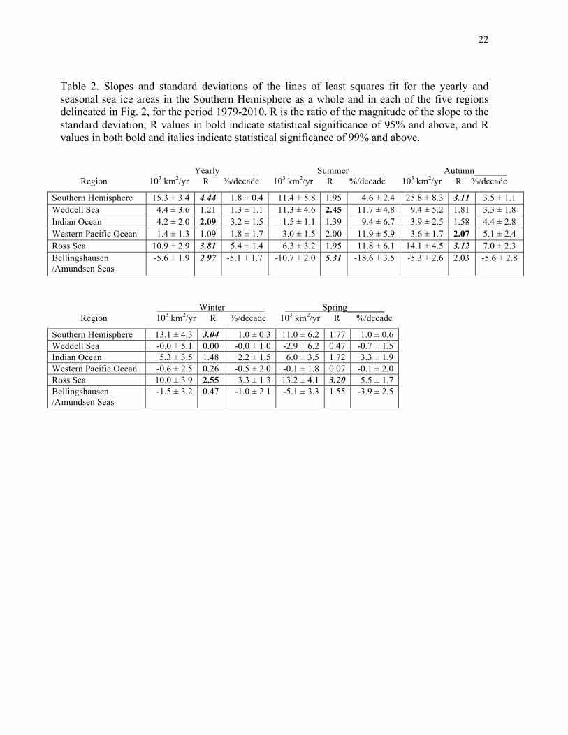
Table 2. Slopes and standard deviations of the lines of least squares fit for the yearly and seasonal sea ice areas in the Southern Hemisphere as a whole and in each of the five regions delineated in Fig. 2, for the period 1979-2010. R is the ratio of the magnitude of the slope to the standard deviation; R values in bold indicate statistical significance of 95% and above, and R values in both bold and italics indicate statistical significance of 99% and above.

Yearly Summer Autumn_______ Region 103 km2/yr R %/decade 103 km2/yr R %/decade 103 km2/yr R %/decade

Southern Hemisphere 15.3 ± 3.4 4.44 1.8 ± 0.4 11.4 ± 5.8 1.95 4.6 ± 2.4 25.8 ± 8.3 3.11 3.5 ± 1.1 Weddell Sea 4.4 ± 3.6 1.21 1.3 ± 1.1 11.3 ± 4.6 2.45 11.7 ± 4.8 9.4 ± 5.2 1.81 3.3 ± 1.8 Indian Ocean 4.2 ± 2.0 2.09 3.2 ± 1.5 1.5 ± 1.1 1.39 9.4 ± 6.7 3.9 ± 2.5 1.58 4.4 ± 2.8 Western Pacific Ocean 1.4 ± 1.3 1.09 1.8 ± 1.7 3.0 ± 1.5 2.00 11.9 ± 5.9 3.6 ± 1.7 2.07 5.1 ± 2.4 Ross Sea 10.9 ± 2.9 3.81 5.4 ± 1.4 6.3 ± 3.2 1.95 11.8 ± 6.1 14.1 ± 4.5 3.12 7.0 ± 2.3 Bellingshausen /Amundsen Seas

-5.6 ± 1.9 2.97 -5.1 ± 1.7 -10.7 ± 2.0 5.31 -18.6 ± 3.5 -5.3 ± 2.6 2.03 -5.6 ± 2.8

Winter Spring________ Region 103 km2/yr R %/decade 103 km2/yr R %/decade

Southern Hemisphere 13.1 ± 4.3 3.04 1.0 ± 0.3 11.0 ± 6.2 1.77 1.0 ± 0.6 Weddell Sea -0.0 ± 5.1 0.00 -0.0 ± 1.0 -2.9 ± 6.2 0.47 -0.7 ± 1.5 Indian Ocean 5.3 ± 3.5 1.48 2.2 ± 1.5 6.0 ± 3.5 1.72 3.3 ± 1.9 Western Pacific Ocean -0.6 ± 2.5 0.26 -0.5 ± 2.0 -0.1 ± 1.8 0.07 -0.1 ± 2.0 Ross Sea 10.0 ± 3.9 2.55 3.3 ± 1.3 13.2 ± 4.1 3.20 5.5 ± 1.7 Bellingshausen /Amundsen Seas

-1.5 ± 3.2 0.47 -1.0 ± 2.1 -5.1 ± 3.3 1.55 -3.9 ± 2.5

23

FIGURE CAPTIONS

Figure 1. Maps of Southern Hemisphere February and September sea ice

concentrations, averaged over the years 1979-2010, as derived from SMMR, SSMI, and

SSMIS satellite observations.

Figure 2. Location map, including the identification of the five regions used for the

sea ice analyses.

Figure 3. (a) Monthly average Southern Ocean sea ice extents for November 1978

through December 2010, with an inset showing the average annual cycle, calculated from

SMMR, SSMI, and SSMIS satellite data. (b) Monthly deviations for the sea ice extents of

part a, with the line of least squares fit through the data points and its slope and standard

deviation. (c) Yearly (Y) and seasonally averaged sea ice extents, 1979-2010, with the

corresponding lines of least squares fit. The summer (Su), autumn (A), winter (W), and

spring (Sp) values cover the periods January-March, April-June, July-September, and

October-December, respectively.

Figure 4. Sea ice extent monthly deviation plots, November 1978 through December

2010, calculated from SMMR, SSMI, and SSMIS satellite data, for the following regions

and hemispheric total: (a) Weddell Sea, (b) Indian Ocean, (c) Western Pacific Ocean, (d)

Ross Sea, (e) Bellingshausen/Amundsen Seas, and (f) Southern Hemisphere as a whole.

Figure 5. Monthly sea ice extent trends, 1979-2010, for the following regions and

hemispheric total: (a) Weddell Sea, (b) Indian Ocean, (c) Western Pacific Ocean, (d) Ross

Sea, (e) Bellingshausen/Amundsen Seas, and (f) Southern Hemisphere as a whole.

Figure 6. Same as Figure 3 except for ice areas instead of ice extents.

Figure 7. Same as Figure 4 except for ice areas instead of ice extents.

24

Figure 8. Same as Figure 5 except for ice areas instead of ice extents.

25

Figure 1

26

Figure 2

27

Figure 3

28

Figure 4

29

Figure 5

30

Figure 6

31

Figure 7

32

Figure 8