ant-inspired approach for resource localization in mobile
TRANSCRIPT
UNIVERSITY OF OSLODepartment of Informatics
Ant-InspiredApproach forResourceLocalization inMobile Ad-HocNetworks
Master’s Thesis
Maren Feragen
May 3, 2010


Abstract
Computer networks are constantly emerging, and in today’s world, we seenew needs and new kinds of networks addressing these needs. Situations suchas emergency and rescue operations present a demand for mobile ad-hoc net-works, a kind of networks with fundamentally different characteristics thantraditional wired networks. Scarce resources and possibly low connectivitycall for new techniques and approaches to traditional problems.
Where possible, resource localization tools will probably be included inthe applications needing it, enabling them to tune the search to the ap-plications needs and characteristics. However, such needs are not alwayspossible to predict a priori, and we then need a system enabling nodes to au-tonomously localize needed resources that are not present in the node itself.In this thesis, we propose a general-purpose resource localization solution formobile ad-hoc networks.
Nodes in mobile ad-hoc networks should function autonomously withas little outside intervention as possible, preserving the self-* properties.Such systems are common in nature, and may be used as inspiration whendesigning computer systems. In this thesis, we look at how stigmergy — theforaging behavior of ants — may be used to localize resources in a mobile ad-hoc network. When walking between their nest and a food source, ants leavepheromone trails on the ground, and by probabilistically choosing brancheswith the most pheromone, they are able to find the shortest path betweentheir nest and the food. This behavior has inspired a lot of solutions tooptimization problems like routing.
We have designed and implemented a system exploiting what we call op-posite stigmergy, where artificial ants are released from a resource-requestingnode and at each intermediate node probabilistically choose the least recentlyused neighbor as next hop. This makes ants search every nook and cranny ofthe network, as opposed to regular ant-inspired algorithms, where ants areconcentrated on one or a few most optimal paths.
Our preliminary performance tests show that our ant-inspired approachhas, if tuned correctly, the potential to outperform the much simpler flooding-based solution in certain scenarios. The ant solution has shown to be able tolocalize resources with less sent and received messages if more than one noderequests the same (or similar) resources. For scenarios where nodes have ahigh number of neighbors, however, we see that the ant approach requiresa lot of time and resources to localize a resource. We also suggest a fewpotential fixes that may be able to lower both the response time as well asthe resource consumption, enabling the ant solution to perform even better.


Acknowledgements
First and foremost, I want to thank my supervisor, Ellen Munthe-Kaas, forgiving me excellent support, guidance, ideas; and not least for introducingme to the somewhat out of the ordinary — but very intriguing — topic forthis thesis. I also want to thank Matija Pužar and Piotr Kamisinski forhelping me out during the test phase and for patiently assisting me all thosetimes my code or computer didn’t do what I wanted it to. Finally, I thankmy friends and family for their support and encouragement during the workwith this thesis.
Maren FeragenUniversity of Oslo
May 3, 2010

Contents
1 Introduction 11.1 Background . . . . . . . . . . . . . . . . . . . . . . . . . . . . 2
1.2 Motivation . . . . . . . . . . . . . . . . . . . . . . . . . . . . . 3
1.2.1 Rescue Operations — A Case Study . . . . . . . . . . 3
1.2.2 Application Domain . . . . . . . . . . . . . . . . . . . 4
1.3 Problem Description . . . . . . . . . . . . . . . . . . . . . . . 5
1.4 The SIRIUS Project . . . . . . . . . . . . . . . . . . . . . . . 6
1.5 Outline . . . . . . . . . . . . . . . . . . . . . . . . . . . . . . 6
2 Mobile Ad-Hoc Networks and Autonomic Networking 92.1 Mobile Ad-Hoc Networks . . . . . . . . . . . . . . . . . . . . . 9
2.1.1 Characteristics of Mobile Ad-Hoc Networks . . . . . . 9
2.1.2 Issues in Mobile Ad-Hoc Networks . . . . . . . . . . . 10
2.1.3 Routing in Mobile Ad-Hoc Networks . . . . . . . . . . 12
2.1.4 Applications . . . . . . . . . . . . . . . . . . . . . . . . 16
2.2 Autonomic Networking . . . . . . . . . . . . . . . . . . . . . . 17
2.2.1 Autonomic Networks . . . . . . . . . . . . . . . . . . . 17
2.2.2 Self-*: Properties of an Autonomic Network . . . . . . 17
2.2.3 Autonomy in MANETs . . . . . . . . . . . . . . . . . 20
3 A Bug’s Life 213.1 Communication . . . . . . . . . . . . . . . . . . . . . . . . . . 21
3.2 Stigmergy and Ant Colony Optimization . . . . . . . . . . . . 22
3.2.1 Pheromones . . . . . . . . . . . . . . . . . . . . . . . . 23
3.2.2 Ants and Their Pheromones . . . . . . . . . . . . . . . 23
3.2.3 Ant Colony Optimization . . . . . . . . . . . . . . . . 25
4 ACO Approaches to Some Traditional Problems 274.1 The Ant Colony Optimization Metaheuristic . . . . . . . . . . 27
4.2 The Traveling Salesman Problem . . . . . . . . . . . . . . . . 29
4.2.1 Solving the TSP with ACO Algorithms . . . . . . . . 29
4.2.2 AntSystem . . . . . . . . . . . . . . . . . . . . . . . . 30
4.3 The Routing Problem . . . . . . . . . . . . . . . . . . . . . . 31

vi Contents
4.3.1 AntNet — Routing in Traditional Networks . . . . . . 324.3.2 AntHocNet — Routing in Mobile Ad-Hoc Networks . 35
5 Design 395.1 Goal . . . . . . . . . . . . . . . . . . . . . . . . . . . . . . . . 395.2 Assumptions . . . . . . . . . . . . . . . . . . . . . . . . . . . 39
5.3 Requirements . . . . . . . . . . . . . . . . . . . . . . . . . . . 40
5.4 General Idea . . . . . . . . . . . . . . . . . . . . . . . . . . . 40
5.5 Issues . . . . . . . . . . . . . . . . . . . . . . . . . . . . . . . 42
5.5.1 Scheduling . . . . . . . . . . . . . . . . . . . . . . . . . 42
5.5.2 Communication . . . . . . . . . . . . . . . . . . . . . . 43
5.5.3 Supported Network Topology . . . . . . . . . . . . . . 45
5.5.4 Resources . . . . . . . . . . . . . . . . . . . . . . . . . 45
5.5.5 Pheromone Traces . . . . . . . . . . . . . . . . . . . . 46
5.5.6 Ants . . . . . . . . . . . . . . . . . . . . . . . . . . . . 48
5.6 The Localization Algorithm . . . . . . . . . . . . . . . . . . . 52
6 Implementation 556.1 Remarks . . . . . . . . . . . . . . . . . . . . . . . . . . . . . . 55
6.2 Programming Language . . . . . . . . . . . . . . . . . . . . . 56
6.3 Developing for NEMAN . . . . . . . . . . . . . . . . . . . . . 56
6.4 The sockaddr_in structure . . . . . . . . . . . . . . . . . . . . 56
6.5 Logging . . . . . . . . . . . . . . . . . . . . . . . . . . . . . . 57
6.6 Neighbor Information . . . . . . . . . . . . . . . . . . . . . . . 58
6.6.1 Topology Information Retrieval . . . . . . . . . . . . . 58
6.6.2 Neighbor Registry . . . . . . . . . . . . . . . . . . . . 59
6.6.3 Topology Changes During Resource Localization . . . 59
6.7 Resources . . . . . . . . . . . . . . . . . . . . . . . . . . . . . 61
6.7.1 Local Resource Information . . . . . . . . . . . . . . . 61
6.7.2 Resource Sharing . . . . . . . . . . . . . . . . . . . . . 61
6.7.3 Resource Location Info . . . . . . . . . . . . . . . . . . 62
6.8 Pheromone Traces . . . . . . . . . . . . . . . . . . . . . . . . 63
6.8.1 Pheromone Data Structure . . . . . . . . . . . . . . . 63
6.8.2 Pheromone Initialization . . . . . . . . . . . . . . . . . 65
6.8.3 Pheromone Updates . . . . . . . . . . . . . . . . . . . 65
6.9 Ants and Ant Memory . . . . . . . . . . . . . . . . . . . . . . 65
6.9.1 Choosing the Next Hop . . . . . . . . . . . . . . . . . 66
6.9.2 Loop Elimination . . . . . . . . . . . . . . . . . . . . . 68
6.9.3 Ant Communication . . . . . . . . . . . . . . . . . . . 68
6.10 Resource Localization . . . . . . . . . . . . . . . . . . . . . . 68
6.10.1 Search Initiation . . . . . . . . . . . . . . . . . . . . . 68
6.10.2 Search Termination . . . . . . . . . . . . . . . . . . . . 69
6.11 Utilities . . . . . . . . . . . . . . . . . . . . . . . . . . . . . . 69
6.12 Program Flow . . . . . . . . . . . . . . . . . . . . . . . . . . . 70

Contents vii
6.12.1 Threads . . . . . . . . . . . . . . . . . . . . . . . . . . 70
7 Test Setup 717.1 Evaluation Techniques . . . . . . . . . . . . . . . . . . . . . . 71
7.2 Testing Environment . . . . . . . . . . . . . . . . . . . . . . . 737.2.1 Simulation vs Emulation . . . . . . . . . . . . . . . . . 73
7.2.2 ns-2 . . . . . . . . . . . . . . . . . . . . . . . . . . . . 73
7.2.3 NEMAN . . . . . . . . . . . . . . . . . . . . . . . . . . 73
7.2.4 OLSR daemon . . . . . . . . . . . . . . . . . . . . . . 74
7.3 Emulation and Analysis Tools . . . . . . . . . . . . . . . . . . 74
7.3.1 setdest . . . . . . . . . . . . . . . . . . . . . . . . . . . 74
7.3.2 tcpdump . . . . . . . . . . . . . . . . . . . . . . . . . . 75
7.4 A Flooding Solution . . . . . . . . . . . . . . . . . . . . . . . 75
7.4.1 Issues with Flooding . . . . . . . . . . . . . . . . . . . 75
7.4.2 Flooded Requests . . . . . . . . . . . . . . . . . . . . . 76
7.5 Monitoring . . . . . . . . . . . . . . . . . . . . . . . . . . . . 77
7.6 Metrics . . . . . . . . . . . . . . . . . . . . . . . . . . . . . . 77
7.6.1 Response Time . . . . . . . . . . . . . . . . . . . . . . 78
7.6.2 Resource Usage and Utilization . . . . . . . . . . . . . 80
7.7 Test Scenarios . . . . . . . . . . . . . . . . . . . . . . . . . . . 83
7.7.1 Chain Scenario . . . . . . . . . . . . . . . . . . . . . . 83
7.7.2 Grid Scenario . . . . . . . . . . . . . . . . . . . . . . . 83
7.7.3 Mobility Scenario . . . . . . . . . . . . . . . . . . . . . 84
7.8 Test Scenario Implementation . . . . . . . . . . . . . . . . . . 85
7.8.1 Static Scenarios . . . . . . . . . . . . . . . . . . . . . . 86
7.8.2 Mobility Scenario . . . . . . . . . . . . . . . . . . . . . 86
7.9 Workload . . . . . . . . . . . . . . . . . . . . . . . . . . . . . 87
7.9.1 Parameters . . . . . . . . . . . . . . . . . . . . . . . . 89
7.9.2 Scenario Properties . . . . . . . . . . . . . . . . . . . . 89
7.9.3 Single Localization . . . . . . . . . . . . . . . . . . . . 90
7.9.4 Location Learning . . . . . . . . . . . . . . . . . . . . 91
8 Performance Evaluation 958.1 Influencing Factors . . . . . . . . . . . . . . . . . . . . . . . . 95
8.1.1 Topology Initialization and Updates . . . . . . . . . . 95
8.1.2 Time Inaccuracy . . . . . . . . . . . . . . . . . . . . . 96
8.1.3 Average Neighborhood Size . . . . . . . . . . . . . . . 96
8.2 Results — Response Time . . . . . . . . . . . . . . . . . . . . 97
8.2.1 Single Localization . . . . . . . . . . . . . . . . . . . . 97
8.2.2 Location Learning . . . . . . . . . . . . . . . . . . . . 100
8.2.3 Conclusion . . . . . . . . . . . . . . . . . . . . . . . . 102
8.3 Results — Bandwidth Usage . . . . . . . . . . . . . . . . . . 103
8.3.1 Single Localization . . . . . . . . . . . . . . . . . . . . 103
8.3.2 Location Learning . . . . . . . . . . . . . . . . . . . . 105

viii Contents
8.3.3 Conclusion . . . . . . . . . . . . . . . . . . . . . . . . 107
8.4 Results — Processing Power Usage . . . . . . . . . . . . . . . 108
8.4.1 Single Localization . . . . . . . . . . . . . . . . . . . . 109
8.4.2 Location Learning . . . . . . . . . . . . . . . . . . . . 109
8.4.3 Conclusion . . . . . . . . . . . . . . . . . . . . . . . . 110
8.5 Results — Processing Power Utilization . . . . . . . . . . . . 110
8.5.1 Single Localization . . . . . . . . . . . . . . . . . . . . 111
8.5.2 Location Learning . . . . . . . . . . . . . . . . . . . . 111
8.5.3 Conclusion . . . . . . . . . . . . . . . . . . . . . . . . 112
9 Conclusion and Further Work 1139.1 Contribution . . . . . . . . . . . . . . . . . . . . . . . . . . . 113
9.2 Performance Evaluation . . . . . . . . . . . . . . . . . . . . . 114
9.3 Critical Assessments . . . . . . . . . . . . . . . . . . . . . . . 115
9.4 Further Work . . . . . . . . . . . . . . . . . . . . . . . . . . . 116
9.4.1 Resource Localization in Sparse Networks . . . . . . . 116
9.4.2 Resource Goodness . . . . . . . . . . . . . . . . . . . . 117
9.4.3 Further Implementation, Testing and Analysis . . . . . 118
Bibliography 120
Appendices 127
A A Sample Scenario File 127A.1 Chain Scenario . . . . . . . . . . . . . . . . . . . . . . . . . . 127
B The Flooding Solution 129B.1 Data structures . . . . . . . . . . . . . . . . . . . . . . . . . . 129
B.1.1 Logging . . . . . . . . . . . . . . . . . . . . . . . . . . 130
B.1.2 Program Flow . . . . . . . . . . . . . . . . . . . . . . . 130
C Source Code 131C.1 Program Layout — Ant Solution . . . . . . . . . . . . . . . . 131
C.2 Program Layout — Flooding Solution . . . . . . . . . . . . . 131
C.3 Building the Source Code . . . . . . . . . . . . . . . . . . . . 132
C.4 Running the Source Code . . . . . . . . . . . . . . . . . . . . 132
D Code Examples 133D.1 send_forward_ant() . . . . . . . . . . . . . . . . . . . . . . . 133
D.2 receive_ants() . . . . . . . . . . . . . . . . . . . . . . . . . . . 134
D.3 handle_received_ant() . . . . . . . . . . . . . . . . . . . . . . 135
D.4 handle_forward_ant() . . . . . . . . . . . . . . . . . . . . . . 136
D.5 handle_backward_ant() . . . . . . . . . . . . . . . . . . . . . 136

Contents ix
E CD Contents 139E.1 /implementation . . . . . . . . . . . . . . . . . . . . . . . . . 139
E.1.1 /implementation/ant_solution . . . . . . . . . . . . . 139E.1.2 /implementation/flooding_solution . . . . . . . . . . . 139
E.2 /test_setup . . . . . . . . . . . . . . . . . . . . . . . . . . . . 139E.2.1 /test_setup/scenarios . . . . . . . . . . . . . . . . . . 140
E.3 /analysis . . . . . . . . . . . . . . . . . . . . . . . . . . . . . . 140


List of Figures
2.1 A simple MANET . . . . . . . . . . . . . . . . . . . . . . . . 10
2.2 Sample MANET before and after partitioning . . . . . . . . . 11
2.3 Message forwarding in LSR versus OLSR . . . . . . . . . . . . 14
2.4 Epidemic routing in a MANET with two partitions . . . . . . 15
3.1 Two kinds of trail-leaving ants . . . . . . . . . . . . . . . . . . 24
3.2 Ant colony is unable to converge to shortest path . . . . . . . 25
4.1 Pseudo-code for the ACO metaheuristic . . . . . . . . . . . . 29
5.1 The disadvantage of backward ants depositing pheromones . . 47
5.2 Allowing ant loops increases network utilization . . . . . . . . 51
5.3 Pseudo-code for the ant solution . . . . . . . . . . . . . . . . 53
6.1 C code for binding a socket to a specific device . . . . . . . . 57
6.2 sockaddr_in structure . . . . . . . . . . . . . . . . . . . . . . 57
6.3 Neighbor structure . . . . . . . . . . . . . . . . . . . . . . . . 59
6.4 Backward ant — neighbor lost . . . . . . . . . . . . . . . . . 60
6.5 Forward ant — neighbor lost . . . . . . . . . . . . . . . . . . 60
6.6 A sample resource file . . . . . . . . . . . . . . . . . . . . . . 61
6.7 Resource structure . . . . . . . . . . . . . . . . . . . . . . . . 62
6.8 Resource info structure . . . . . . . . . . . . . . . . . . . . . . 62
6.9 Two-dimensional linked list structure . . . . . . . . . . . . . . 64
6.10 Pheromone structure . . . . . . . . . . . . . . . . . . . . . . . 64
6.11 Ant structure . . . . . . . . . . . . . . . . . . . . . . . . . . . 66
6.12 Neighbor probability structure . . . . . . . . . . . . . . . . . . 67
6.13 Loop elimination . . . . . . . . . . . . . . . . . . . . . . . . . 68
6.14 Doubly linked list structure . . . . . . . . . . . . . . . . . . . 70
7.1 Response time metric . . . . . . . . . . . . . . . . . . . . . . . 78
7.2 Different interpretations of the response time metric . . . . . 78
7.3 Chain topology . . . . . . . . . . . . . . . . . . . . . . . . . . 83
7.4 Grid topology . . . . . . . . . . . . . . . . . . . . . . . . . . . 84
7.5 Mobility topology . . . . . . . . . . . . . . . . . . . . . . . . . 85

xii List of Figures
7.6 Chain topology NEMAN screenshot . . . . . . . . . . . . . . 867.7 Grid topology NEMAN screenshot . . . . . . . . . . . . . . . 877.8 Mobility topology NEMAN screenshots . . . . . . . . . . . . . 887.9 Chain topology with one requesting node . . . . . . . . . . . 907.10 Grid topology with one requesting node . . . . . . . . . . . . 917.11 Mobility topology with one requesting node . . . . . . . . . . 927.12 Grid topology with three requesting nodes . . . . . . . . . . . 937.13 Mobility topology with five requesting nodes . . . . . . . . . . 94
8.1 Number of neighbors per second in the mobility scenarios . . 988.2 Response time in grid scenario with location learning . . . . . 1018.3 Response time in M-dense scenario with location learning . . 1018.4 Response time in M-sparse scenario with location learning . . 1028.5 Message sizes for flooding and ant solutions . . . . . . . . . . 1058.6 Utilization in each single location scenario . . . . . . . . . . . 1108.7 Utilization in each location learning scenario . . . . . . . . . . 111
B.1 Flood_package structure . . . . . . . . . . . . . . . . . . . . . 129B.2 Node_seq structure . . . . . . . . . . . . . . . . . . . . . . . 130B.3 Request_answer structure . . . . . . . . . . . . . . . . . . . . 130
List of Tables
8.1 Neighbors in the mobility scenarios . . . . . . . . . . . . . . . 988.2 Number of hops used in each scenario . . . . . . . . . . . . . 998.3 Time spent in each scenario . . . . . . . . . . . . . . . . . . . 998.4 Messages sent and received in single localization scenarios . . 1048.5 Bytes sent and received in single localization scenarios . . . . 1048.6 Messages sent and received in location learning scenarios . . . 1068.7 Bytes sent and received in location learning scenarios . . . . . 106


List of Abbreviations
ACO Ant Colony Optimization
AODV Ad Hoc On Demand Distance Vector
AS AntSystem
CSMA/CA Carrier Sense Multiple Access / Collision Avoidance
CTS Clear To Send
DCF Distributed Coordination Function
DMMS Distributed Multimedia Systems
IEEE Institute of Electrical and Electronics Engineers
LSR Link-State Routing
MANET Mobile Ad-Hoc Network
MPR Multi-Point Relay
OLSR Optimized Link State Routing
RREP Route Reply
RREQ Route Request
RTS Ready To Send
SIRIUS Sensing, Adapting and Protecting Pervasive Information Spaces
TCP Transmission Control Protocol
TSP Traveling Salesman Problem
UPD User Datagram Protocol
WAN Wide Area Network


Chapter 1
Introduction
”I’m not afraid of computers taking over the world. They’re
just sitting there. I can hit them with a two by four.”
— Thom Yorke
In mobile ad-hoc networks, nodes should function autonomously, andthey should be able to adapt to their environment and any changes in itwithout any external intervention. For nodes to be able to adapt to theirenvironment, they obviously need to have a certain knowledge about theirenvironment and to somehow be aware of any changes within this environ-ment.
The environment of a node in a mobile ad-hoc network is made up of thenodes in the network, and how these are placed, their mobility, speed andany other characteristics that a node may enclose, such as what resources arepresent at which nodes in the network. One kind of environmental changesis thus changes in the network topology, which may occur frequently becauseof node mobility. Another possible environmental change is changes to theresource situation at one node.
As we are dealing with mobile ad-hoc networks, it is important that nodesare able to monitor their environment and perform any required adaptationswithout any external intervention — they need to function autonomously.Autonomous, self-adapting systems are common in nature, and have beenused as inspiration for solutions to a lot of computer-related problems, es-pecially optimization problems. The most common source of inspiration isants and their foraging behavior. A lot of research has been done on ant-inspired approaches to optimization problems like the routing problem, bothin traditional, wired networks as well as in mobile ad-hoc networks.
With this thesis, we want to look at how ants and their behavior may beused as inspiration for other kinds of problems, and to find out if such ap-proaches may be feasible also in other scenarios than the typical optimization
2 Chapter 1
problems. As our application domain we have chosen resource localization inmobile ad-hoc networks. The purpose of the resulting solution is to enablenodes to search for any resource at any time without the need for any priorknowledge about which resources will be requested or when requests may beissued beforehand. This way, nodes may issue searches for a given resourcewhenever they discover a need for knowledge about the resource situationwithin the network.
1.1 Background
Over the last few decades, there has been a shift from the more traditionalway of networking, with a static, wired infrastructure connecting relativelyfew and homogeneous nodes, to a more widespread, dynamic and thus morecomplex infrastructure. We now see large networks, a mix of wired andwireless infrastructure, connecting a large number of more heterogeneousnodes. However, we also see a need for networks in places that networkinghas before been unthinkable, as there exists no infrastructure, nor, perhaps,any plans of ever making one. Examples of places like this may be sparselypopulated, desolate regions and third world countries, but also in more urbansettings like in tunnels, where outside signals would have a small chance ofreaching in.
For this purpose, a new kind of networks, called Mobile Ad-Hoc Networks(MANETs) have been introduced. A MANET is an autonomous network ofmobile, wireless nodes. In a MANET, there is no fixed infrastructure, andall nodes in the MANET thus need to be able to work both as an end systemand a router, in order to make it possible for nodes not within range of eachother to communicate with each other via other nodes in the MANET.
In situations like emergency and rescue operations, it is of great impor-tance to set up a well functioning network as fast as possible, in order to beable to exchange information about the emergency and potential victims be-tween the rescue workers as fast as possible. Because no fixed infrastructureis needed for establishing MANETs, they can quickly be established, and arethus thought of as a good solution in such situations.
Nodes in a MANET may be highly mobile, and the topology within thenetwork may thus change rapidly, as nodes move in and out of range ofeach other. Also, nodes in a MANET typically have scarce resources, suchas bandwidth, battery power and CPU. These characteristics put harderrequirements on the algorithms used to maintain this kind of networks.
Typical for the more traditional networks is a human network adminis-trator running the network, making sure everything works as desired, doingthe necessary adjustments and repairs. As networks are growing larger andmore complex, along with the introduction of MANETs, the workload onthe human administrator increases or becomes unfeasible, as there might

Introduction 3
not be an obvious candidate for the network administrator role. It is alsogetting harder and harder to anticipate when implementing systems whatoptimizations and adaptations will be needed at runtime. Thus, with to-day’s new networking world, it is desired to automate these processes: Tolet the network itself do the necessary adaptation and optimization, to makethe necessary changes on itself when needed, to protect itself from threats,and to repair itself when needed.
1.2 Motivation
As mentioned above, MANETs may be used where there is no fixed infra-structure. The lack of infrastructure may be due to remote location, andthus few or no possible users, restricted economy and thus the power tobuild the needed infrastructure, but also unforeseen incidents such as a fire,an earthquake or some other natural disaster.
In many of these settings, such as in rural locations, networking is not aprerequisite. However, situations may arise where being able to communicateefficiently would be highly advantageous. Examples of such situations areemergency operations, both in rural locations as well as more urban locationssuch as tunnels, and during battlefield operations. MANETs may also beused in less critical situations, for example in wildlife tracking [19].
1.2.1 Rescue Operations — A Case Study
In April 1998, the personnel on a metro train with several hundred persons onboard discovered a fire in Majorstutunnelen, a 1790 metre long metro tunnelin the center of Oslo [12]. The personnel tried contacting their supervisors,but with no luck, and let their passengers off inside the tunnel, hoping theywould get out safely without supervision. At the same time, there was alsoanother train inside the same tunnel. As no one was able to contact anyoneon the outside, the personnel in the other train knew nothing about thefire until they saw people walking towards them along the tracks inside thetunnel. Luckily, the driver was able to stop the train, avoiding to hit any ofthe passengers from the other train.
In such a scenario, the ability to communicate, both with someone on theoutside as well as with the personnel on board other trains nearby, is crucial.In our scenario, luckily, no one was physically hurt, and everyone managedto get out of the tunnel. The fire turned out to be small, and was shortlyafter extinguished by fire personnel. However, it is not hard to imagine aless happy ending: The fire could have been worse, the driver of the othertrain could have been unable to stop his train in time, people could havebeen hurt by the electric current in the railway tracks. In such a scenario,the amount of rescue personnel involved in the rescue operation might getvery high, as both fire fighters, police personnel and medical personnel may
4 Chapter 1
need to enter the tunnel to contribute. With such an amount of personnelin action, the need for efficient communication is even greater: Who is doingwhat, how many victims are located where, who needs help first, who hasgot what equipment where, and so on.
If all rescue workers carried with them a small device with the ability tocommunicate with other devices, they would be able to set up a MANETwithout much effort, enabling them to exchange messages, pictures, maps,resource information and all other kinds of information useful to the rescueoperation. They might also place sensors on their patients, enabling them tomonitor moderately hurt people without being physically close to them. Thesensors could trigger an alarm if the patient’s condition gets worse, tellingmedical personnel to go check up on the patient.
Other sensors and cameras might monitor the tunnel environment withrespect to for example temperature and the amount of poisonous gases in theair inside the tunnel, making sure it is safe to continue the rescue operationinside the tunnel, again giving alerts to the appropriate personnel wheneverthe conditions get worse.
Many of these tasks could be accomplished with the help from existingsystems or even plain communication between the rescue personnel. How-ever, one rescue worker may carry certain kinds of equipment or even knowl-edge that other workers may benefit from. If the resource holder could answerto resource requests without actually having to pick up his or her device andtype an answer, this rescue worker would be free to work with other tasksfor more of the time, making this worker more efficient, possibly saving morelives or in some other way minimizing damage. Thus, we would like a systemwhere one could send a message ”I need resource X”, and the system wouldlocate this resource within the MANET without any human intervention.
1.2.2 Application Domain
A rescue operation is of course not the only domain where such a systemmight be helpful. Any system where one node might need resources notpresent within the node itself would benefit from such a system. However,there are a few characteristics that are common for the kind of applicationdomains the work in this thesis is targeted at. These characteristics putsome restrictions on the solutions developed:
• As resources in a MANET are typically scarce, we would like a solutionwith a high utilization of the present resources: We want as little wasteas possible of both bandwidth as well as processing power.
• MANET node characteristics include frequent joins and leaves as wellas partitioning.
• No other system for sharing and dissemination resource information

Introduction 5
is already present within the system, or the existing solution is notadequate.
The actual consequences of the first two restrictions will be further dis-cussed in later sections, but we do already state that these restrictionsseverely complicate both the design and implementation of systems targetedat MANETs.
If it is possible to predict beforehand what kind of resources might bepresent in the network and what resources may be requested, resource dis-semination and localization tools will probably be included in the system,and may then be tailored to fit the needs and characteristics of the system inquestion. However, it is not always possible to foresee the exact needs anddevelopment of a system. Thus, what we aim to develop in this thesis is asolution for use either when no such tools are available, or as an addition toany existing tools. Thus, we try to develop a general purpose tool that maybe used to look for any resource at any time in any MANET.
1.3 Problem Description
A lot of research has been done on how well biologically inspired algorithmsapply to computer network problems, both in traditional networks as wellas MANETs. These approaches look at how we can make computer systemssimulate behavior seen in the nature. Self-organizing systems exist naturallyin nature, where they function without any external interference or centralcontrol. They adapt to changes around them, making them more robust toenvironmental changes and increasing their own survivability. One exampleof such biological systems is insects, like ant colonies, termites or bees, whocommunicate through stigmergy. The term stigmergy was introduced byGrassé in 1959 [26]. Grassé defined stigmergy as
”Stimulation of workers by the performance they have achieved.”Dorigo et al. [9]
In other words, stigmergy describes insects’ indirect communication medi-ated by changes to the environment. This phenomenon is also referred to asswarm intelligence. In the case of termites and ants, stigmergy is ensuredby depositing the chemical substance pheromone in the environment [36].
Another example is autopoiesis, or self-production, which refers to sys-tems of components that are able to reproduce themselves, and in this wayself-maintain the system [36]. Other such examples exist, such as decrease ofentropy [36], and these natural systems may all be used as inspiration whendesigning autonomous computer systems and networks.
In this thesis, we look at some of the algorithms from the Ant ColonyOptimization [10] research field, and try to map these techniques to ourproblem: Locating a given resource within a MANET. More specifically, we

6 Chapter 1
will look at the behavior of ants during their search for food, and try toexploit the characteristics of their movement in our own search for resourcesin a MANET.
1.4 The SIRIUS Project
This thesis is written as part of the SIRIUS (Sensing, Adapting and Pro-tecting Pervasive Information Spaces) project at the Distributed Multime-dia Systems (DMMS) research group. The project mainly focuses on threechallenges:
• Sensing/monitoring as a high-level service for applications.
• Adaptation through a framework supporting autonomous adjustmentsof all objects in such systems, minimizing unwanted side effects fromindividual adaptations.
• Protection through a tool for identifying and detecting normal as wellas abnormal behavior in the system, perform analysis and carry outcounter efforts demanding a minimal amount of manual intervention.
The project aims to provide concepts and mechanisms for system devel-opers, enabling them to create large-scale pervasive systems. In additionto this, a platform shielding the application developer from the underlyingcomplexities is needed, as one cannot expect every developer to understandand address all issues introduced by the new turn in networking.
This thesis is a contribution to the second point above; adaptation. Re-source localization is to be done autonomously, and nodes holding and seek-ing resource information need to be able to adapt to any changes in theirenvironment, such as node mobility, which may lead to resource-holdingnodes moving or even leaving the MANET. Also, by gathering resource in-formation, nodes may get information about the status of the network, andmay thus be able to adapt to any changes without any outside intervention.
1.5 Outline
The rest of this thesis is organized as follows: Chapter 2 provides a thor-ough explanation of Mobile Ad-Hoc Networks and autonomic networking.In Chapter 3, we look at ants and stigmergy, the biological phenomenonthat is the inspiration of our resource localization system. Chapter 4 takesa deeper look at how ant behavior may be exploited to make solutions tosome traditional computer network problems.
Our resource localization design is explained in Chapter 5, whereas themore technical details of our implementation are provided in Chapter 6.

Introduction 7
The test setup used in our experiments, along with a presentation of someof the most important tools used during the testing, is provided in Chapter7. The test results and system evaluation follows in Chapter 8. At last, weconclude and present further work in Chapter 9.
The thesis also includes four appendices. Appendix A contains a sam-ple NEMAN scenario file with additional comments and explanations. InAppendix B, we explain some of the details of the flooding solution usedfor comparison during the performance analysis, whereas Appendix C pro-vides an overview of the source code of both the ant solution as well as theflooding solution. Appendix D lists some of the most important parts of thesource code for our application. The final appendix, Appendix E explainsthe content of the CD appended to this thesis.


Chapter 2
Mobile Ad-Hoc Networks and
Autonomic Networking
”Never underestimate the bandwidth of a station wagon full
of tapes hurtling down the highway.”
— Andrew S. Tanenbaum
In this chapter, we will go through a few topics relevant for the under-standing of the rest of the thesis. First, we provide a detailed explanation ofmobile ad-hoc networks, some issues, their applications and a few relevantrouting protocols. Then we also give an overview on autonomic networkingand self-* systems.
2.1 Mobile Ad-Hoc Networks
2.1.1 Characteristics of Mobile Ad-Hoc Networks
A Mobile Ad-Hoc Network (MANET) is a collection of mobile, autonomousnodes, together forming a network without using any fixed infrastructure andwithout any outside intervention [13, 38]. Typically, there is no centralizedcontrol, and the network is thus dependent of node cooperation to functionproperly.
Because of the lack of fixed infrastructure, each node is acting as both anend node as well as a router, cooperating on the task of getting each messagefrom source to destination. This means that every node needs to run the(same) routing protocol, which puts a bit of extra load on the nodes.
Each node will have a neighborhood, meaning a set of neighbors, whichare the nodes that are within range of the node and thus may be reachedwith direct communication. All other nodes are outside range, and may thusonly be reached with the help from indirect communication, meaning that
10 Chapter 2
AB
C D
E
F
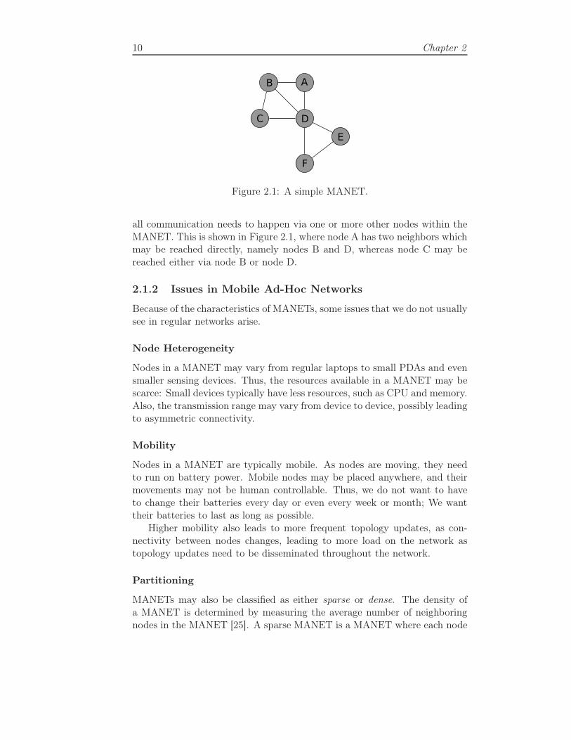
Figure 2.1: A simple MANET.
all communication needs to happen via one or more other nodes within theMANET. This is shown in Figure 2.1, where node A has two neighbors whichmay be reached directly, namely nodes B and D, whereas node C may bereached either via node B or node D.
2.1.2 Issues in Mobile Ad-Hoc Networks
Because of the characteristics of MANETs, some issues that we do not usuallysee in regular networks arise.
Node Heterogeneity
Nodes in a MANET may vary from regular laptops to small PDAs and evensmaller sensing devices. Thus, the resources available in a MANET may bescarce: Small devices typically have less resources, such as CPU and memory.Also, the transmission range may vary from device to device, possibly leadingto asymmetric connectivity.
Mobility
Nodes in a MANET are typically mobile. As nodes are moving, they needto run on battery power. Mobile nodes may be placed anywhere, and theirmovements may not be human controllable. Thus, we do not want to haveto change their batteries every day or even every week or month; We wanttheir batteries to last as long as possible.
Higher mobility also leads to more frequent topology updates, as con-nectivity between nodes changes, leading to more load on the network astopology updates need to be disseminated throughout the network.
Partitioning
MANETs may also be classified as either sparse or dense. The density ofa MANET is determined by measuring the average number of neighboringnodes in the MANET [25]. A sparse MANET is a MANET where each node
Mobile Ad-Hoc Networks and Autonomic Networking 11
AB
C D
E
F
(a) Before partitioning.
A
B
C
D
E
F
(b) After partitioning.
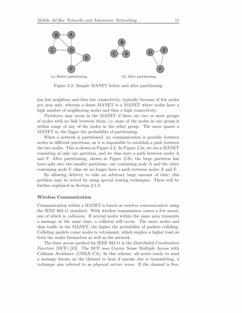
Figure 2.2: Sample MANET before and after partitioning
has few neighbors and thus low connectivity, typically because of few nodesper area unit, whereas a dense MANET is a MANET where nodes have ahigh number of neighboring nodes and thus a high connectivity.
Partitions may occur in the MANET if there are two or more groupsof nodes with no link between them, i.e. none of the nodes in one group iswithin range of any of the nodes in the other group. The more sparse aMANET is, the bigger the probability of partitioning.
When a network is partitioned, no communication is possible betweennodes in different partitions, as it is impossible to establish a path betweenthe two nodes. This is shown in Figure 2.2. In Figure 2.2a, we see a MANETconsisting of only one partition, and we thus have a path between nodes Aand F. After partitioning, shown in Figure 2.2b, the large partition hasbeen split into two smaller partitions, one containing node A and the othercontaining node F, thus we no longer have a path between nodes A and F.
By allowing delivery to take an arbitrary large amount of time, thisproblem may be solved by using special routing techniques. These will befurther explained in Section 2.1.3.
Wireless Communication
Communication within a MANET is based on wireless communication usingthe IEEE 802.11 standard. With wireless transmission comes a few issues,one of which is collisions. If several nodes within the same area transmitsa message at the same time, a collision will occur. The more nodes andthus traffic in the MANET, the higher the probability of packets colliding.Colliding packets cause nodes to retransmit, which implies a higher load onboth the nodes themselves as well as the network.
The basic access method for IEEE 802.11 is the Distributed CoordinationFunction (DCF) [45]. The DCF uses Carrier Sense Multiple Access withCollision Avoidance (CSMA/CA). In this scheme, all nodes ready to senda message listens on the channel to hear if anyone else is transmitting, atechnique also referred to as physical carrier sense. If the channel is free,
12 Chapter 2
the node may send. If not, the node must wait until it is, and then entera random back off procedure where it waits for a random period of time.The random back off procedure is used to make sure several nodes don’tstart transmitting at the same time immediately after the previous trans-mission was done. Because of this, however, in a dense network with a largeamount of transmissions, nodes will often have to wait before they may sendmessages.
However, this approach assumes that all nodes are within range of eachother, a rather unrealistic assumption. To solve this problem, often referredto as the hidden node problem, a carrier sense mechanism called virtual car-rier sense is also used. In order to avoid collisions, a node wanting to sendsomething must reserve the medium for a specified amount of time by trans-mitting a ready to send frame. If the destination node is ready to receive, itreplies with a clear to send frame. All nodes within range of either senderor receiver will hear at least one of these two, and will thus know that themedium is occupied for the reserved time period.
This procedure makes the probability of a collision smaller, as collisionswill only happen if two nodes decide to send a message at the exact samepoint in time. However, it might also make nodes wait quite some timebefore they get to send their messages.
2.1.3 Routing in Mobile Ad-Hoc Networks
Nodes in a MANET may move rapidly and unpredictably. This, togetherwith the restricted resources within a MANET, puts higher restrictions ona MANET routing protocol than on a regular routing protocol designed fortraditional networks:
• The protocol must not use too much bandwidth on route establishmentand maintenance.
• The protocol must adapt fast to topology changes as well as traffic andpropagation changes.
A wide extent of protocols for routing in MANETs have been developed.These may be classified according to several criteria [13]:
• Communication model: Decides if the protocol is designed for sin-gle channel or multi-channel communication. Multi-channel protocolscombine channel assignment and routing functionality, whereas in sin-gle channel protocols, nodes communicate over the same logical wirelesschannel. This is the most common communication model.
• Structure: Distinguishes between uniform protocols, where all nodesplay an equal role in the network, and non-uniform protocols, where

Mobile Ad-Hoc Networks and Autonomic Networking 13
only some nodes participate in route computation. As less nodes par-ticipate in route computation, non-uniform protocols may achieve bet-ter scalability than uniform protocols.
• State information: Distinguishes between topology-based and desti-nation-based protocols. In topology-based protocols, which includelink state protocols, all participating nodes maintain large-scale topol-ogy information. In destination-based protocols, on the other hand,nodes maintain only some local topology information. This class ofprotocols includes distance-vector protocols, in which nodes maintaindistance and next hop information for all destinations.
• Scheduling: Routing protocols may be either proactive or reactive. Aproactive protocol keeps routing information for all destinations at alltimes, whereas reactive protocols only compute routes for a destinationupon request. Proactive protocols thus minimize delay in obtaining aroute, but may use significantly more network resources, as routes maybe computed for destinations that no message will ever be destinedfor. The dissemination of route requests in on-demand protocols, onthe other hand, requires a significant amount of flooding, which putsheavy load on the network. Also, as nearby nodes are bound to re-broadcast a message more or less at the same time, there is a greatchance of contention and collisions occurring.
In addition to this, MANETs may also, as mentioned in Section 2.1.2,be classified as either sparse or dense. Routing in dense MANETs is moresimilar to traditional routing than in sparse networks, as network partitioningand merging are fairly infrequent events and thus there is one only partitionthat needs to be considered. With sparse networks and several partitions,however, there is an additional problem regarding how to send messagesfrom one partition to another and how to manage partition merging. Inthe following we will first go through a couple of routing protocols for densenetworks, before we give a few examples on routing in sparse MANETs.
Routing in Dense MANETs
Optimized Link-State Routing Optimized Link State Routing (OLSR)is a non-uniform, neighbor selection based, proactive routing protocol, mean-ing that not all nodes participate in the route computation, and that onlyinformation about a node’s neighbors is disseminated throughout the net-work [13].
OLSR is, as the name implies, an optimized version of link-state rout-ing (LSR), one of the main classes of routing protocols in traditional wired,packet-switched networks. In regular link-state routing, link state informa-tion from each node is distributed to all other nodes in the network upon

14 Chapter 2
(a) Regular link-state routing. (b) Optimized link-state routing.
Figure 2.3: Message forwarding in LSR versus OLSR. Link-state informationfrom the white middle node is broadcast. Light gray nodes forward messages,black nodes do not.
topology changes. The optimization introduced by OLSR imposes distribu-tion of link-state information to only a subset of a node’s neighbors, calledthe node’s multi-point relay (MPR) set. The MPR set for a node is theminimal subset of the node’s neighbors which must re-broadcast a messagefor it to reach all of the node’s two-hop neighbors.
A node’s link-state information is broadcast to all its neighbors, but onlythose in the node’s MPR set re-broadcasts the information, minimizing thenumber of messages sent during route discovery and maintenance. Also, onlythe link-states of the neighbors in a node’s MPR set is advertised, as opposedto the entire set of neighbors. This is sufficient, as each of the node’s two-hopneighbors is a one-hop neighbor of some node in the MPR set [13].
The effect of this optimization is shown in Figure 2.3. Figure 2.3ashows the message forwarding in LSR, where every node re-broadcasts allreceived link-state messages, while Figure 2.3b shows the message forwardingin OLSR, where only members of a node’s MPR set re-broadcasts a link-statemessage.
Ad-Hoc On Demand Distance Vector Routing Ad-hoc On-demandDistance Vector (AODV) is, as opposed to OLSR, a uniform, destination-based, reactive routing protocol [13]. Whenever a node needs a route to acertain destination, it broadcasts a route request (RREQ). The RREQ isre-broadcast at every node until it reaches the correct destination. Then,a route reply (RREP) is sent back towards the source. On the way back,a forward destination vector is created at each intermediate node. Datadestined for the located node then follows the path stated in the forwarddestination vector.
Mobile Ad-Hoc Networks and Autonomic Networking 15
A
BC
D
E
F
(a) Initial state.
A
B
C
D
E
F
(b) Node B has moved towards thesecond partition.
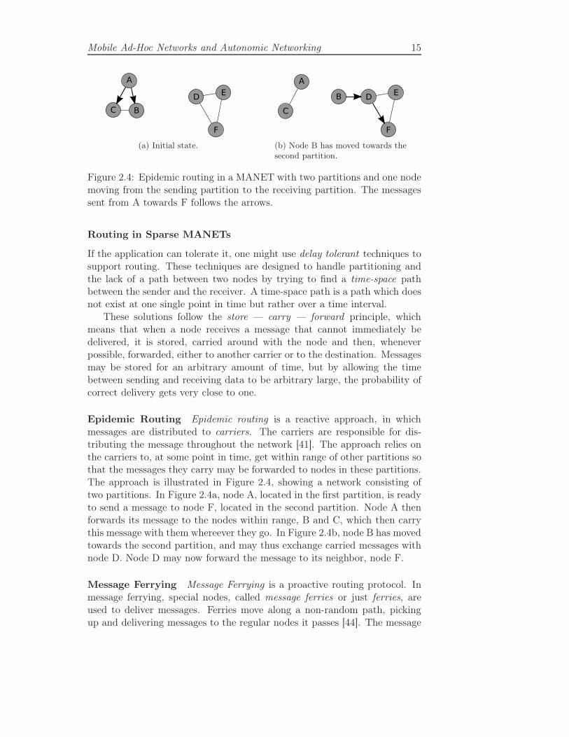
Figure 2.4: Epidemic routing in a MANET with two partitions and one nodemoving from the sending partition to the receiving partition. The messagessent from A towards F follows the arrows.
Routing in Sparse MANETs
If the application can tolerate it, one might use delay tolerant techniques tosupport routing. These techniques are designed to handle partitioning andthe lack of a path between two nodes by trying to find a time-space pathbetween the sender and the receiver. A time-space path is a path which doesnot exist at one single point in time but rather over a time interval.
These solutions follow the store — carry — forward principle, whichmeans that when a node receives a message that cannot immediately bedelivered, it is stored, carried around with the node and then, wheneverpossible, forwarded, either to another carrier or to the destination. Messagesmay be stored for an arbitrary amount of time, but by allowing the timebetween sending and receiving data to be arbitrary large, the probability ofcorrect delivery gets very close to one.
Epidemic Routing Epidemic routing is a reactive approach, in whichmessages are distributed to carriers. The carriers are responsible for dis-tributing the message throughout the network [41]. The approach relies onthe carriers to, at some point in time, get within range of other partitions sothat the messages they carry may be forwarded to nodes in these partitions.The approach is illustrated in Figure 2.4, showing a network consisting oftwo partitions. In Figure 2.4a, node A, located in the first partition, is readyto send a message to node F, located in the second partition. Node A thenforwards its message to the nodes within range, B and C, which then carrythis message with them whereever they go. In Figure 2.4b, node B has movedtowards the second partition, and may thus exchange carried messages withnode D. Node D may now forward the message to its neighbor, node F.
Message Ferrying Message Ferrying is a proactive routing protocol. Inmessage ferrying, special nodes, called message ferries or just ferries, areused to deliver messages. Ferries move along a non-random path, pickingup and delivering messages to the regular nodes it passes [44]. The message

16 Chapter 2
ferrying scheme may be either node initiated or ferry initiated. In a nodeinitiated scheme, the ferry path is known to all nodes. Whenever a nodewants to send something, it moves towards the ferry and delivers its messagesto the ferry when the ferry is within the node’s range.
In the ferry initiated scheme, the ferry moves according to the nodes’needs. Long range radio is used by nodes to inform the ferry that they areready to transmit, instructing the ferry to move towards these nodes.
2.1.4 Applications
The term ad-hoc comes from Latin and means for this purpose. A MANETis a network which may be set up anywhere in a short time, thus being ableto satisfy a demand at short notice. A MANET is set up when no infrastruc-ture is present, thus a MANET is the only possibility for communication, orwhenever the use of present infrastructure is unwanted, for example for se-curity reasons or simply because the existing infrastructure is too expensiveto use.
As there is no centralized control within a MANET, there is no singlepoint of failure. This, together with easy setup and self-organizing nodes,makes MANETs robust to errors and topology changes in terms of enteringand leaving nodes.
MANETs may be suitable in a wide variety of settings. Some typicalapplications include:
• Rescue operations, as illustrated in the motivation for this thesis inSection 1.2.
• Vehicular environments: MANETs may be used in vehicular environ-ments, for example to share information between vehicles. If an acci-dent or some other obstacle has occurred, passing cars may transmitinformation about this to other vehicles on their way to this area, mak-ing them aware of the situation.
• Wildlife monitoring: When monitoring animals in their natural habi-tat, the monitoring should not interfere with the animals’ natural be-havior. Thus, animals should be able to move as usual and should notbe bothered by the sensing device in any way, as this might affect theirbehavior. To achieve this, small sensing devices may be used. Theserun on battery power, and a sensor on one animal may communicateboth with sensors on other animals as well as with base stations ornearby researchers. An example of such a use is ZebraNet [19], whichtracks animal data such as animal location in an area of hundreds orthousands of square kilometers in Kenya.
• Military operations: Military operations often take place in areas whereinfrastructure is non-existing or not suitable to use because of security

Mobile Ad-Hoc Networks and Autonomic Networking 17
issues. The use of a MANET is such scenarios would enable militarypersonnel to communicate, track friendly and enemy forces, and pin-point hazards like minefields. This field is the originator of the basicad-hoc network techniques [38]. MANETs have been used for this pur-pose by the American forces in Iraq [32].
• Home networking and personal entertainment: MANETs may be set upin personal homes, classrooms and public areas to enable for examplefile sharing and gaming.
2.2 Autonomic Networking
2.2.1 Autonomic Networks
As stated in the introduction, what we want is for networks to have theability to organize themselves, and to adapt to the changes in themselvesand their environment. This kind of networks may also be called AutonomicNetworks. Schmid et al. [34] propose the following definition of autonomicsystems:
”An Autonomic System is a system that operates and serves itspurpose by managing its own self without external interventioneven in case of environmental changes.”
In other words, an autonomic network should be able to detect changesand to react upon them.
2.2.2 Self-*: Properties of an Autonomic Network
An autonomic network should be self-organizing. This means that the nodesin the network should organize themselves, and cooperate to form a commu-nity through dynamic role assignment and joint decision making.
Exactly what properties are needed in an autonomic network is discussedin the literature. Schmid et al. state in [34] that all autonomic systems needto exhibit the following minimal set of properties to be able to actuallyfunction autonomically:
• Automatic: The system, here the network nodes, needs to self-controlits internal functions and operations, including bootstrapping, withoutany manual intervention.
• Adaptive: The system needs to be able to change its operation to beable to cope with temporal and spatial changes in its context.
• Aware: At last, the system needs to be able to monitor its context aswell as its internal state.

18 Chapter 2
Serugendo [35], as well as Kephart and Chess [20] identify four funda-mental principles that characterize an autonomic network. These principlesare often called the self-* properties, and are stated as follows:
• Self-configuration:
”Automated configuration of components and systems fol-lows high-level policies. Rest of system adjusts automaticallyand seamlessly.” [20]
This is the first step of self-management within an autonomous net-work. It includes adjusting to new and updated components, as wellas leaving components. For example, the nodes in a network need toadapt to new nodes connecting to the network, as well as nodes leavingthe network.
• Self-optimization:
”Components and systems continually seek opportunities toimprove their own performance and efficiency.” [20]
It is important that all nodes cooperate to keep the network in a statethat is feasible not only for one node, but for the network as a whole.Self-optimization in a network needs to be done at both node andnetwork level. On node level, this means for the node to adapt to thecurrent conditions both in the node’s environment, meaning the restof the network, as well as in the node itself. On network level, thisincludes global optimization through joint decision making.
For example, a node needs to adjust its own resource usage, both ac-cording to its own needs and to the needs of the other nodes in thenetwork. If not, we risk having one node using all the available band-width, leaving all other nodes starving.
• Self-protection:
”System automatically defends against malicious attacks orcascading failures. It uses early warning to anticipate andprevent system wide failures.” [20]
As networks and computer systems in general are getting more andmore complex, the probability of some problem occurring also in-creases. Such problems may be both malicious attacks and normalsoftware and/or hardware failures. To prevent the system or networkfrom complete failure, it is important for the nodes in the network tobe able to protect themselves against these threats.
• Self-healing:

Mobile Ad-Hoc Networks and Autonomic Networking 19
”System automatically detects, diagnoses and repairs local-ized software and hardware problems.” [20]
Self-healing needs, as self-optimization, to be performed at both nodelevel as well as network level. On node level, each node can recover fromfailure by re-configuring itself, e.g. by replacing a failed component withan equivalent, well-functioning component. On network level, recoverymay be accomplished by re-organizing the network, e.g. by replacingfailing nodes with other nodes capable of conducting the same tasks.
For the network nodes to be able to fulfill these four self-* properties,they obviously need quite some knowledge, both about their own state as wellas the network state. Thus, each node also needs a fifth property, namelyself-monitoring — it needs to be able to monitor both itself and the rest ofthe network.
• Self-monitoring: Nodes need to monitor themselves to make sure theyfulfill their objectives. Exactly what to monitor depends on the needsof the node and of the network. Also, the nodes somehow need tomonitor their environment to be able to cooperate with the other nodesin a best possible way. In other words, they need to be context-aware.In [7], Dey gives the following definition of context:
”Context is any information that can be used to characterizethe situation of an entity. An entity is a person, place, orobject that is considered relevant to the interaction betweena user and an application, including the user and applicationsthemselves.”
In [39], metadata, more specifically profiles and policies, are viewed asan emerging approach to support context-awareness. Profiles representdata concerning users, devices, system components and the surround-ing environment. ”Data” may include information like user preferences,device capabilities (available disk space, available memory, installedsoftware) and network conditions. Policies, on the other hand, expresssystem behavior, in terms of the actions subjects can or must operateupon resources. In [37], Sloman distinguishes between two kinds ofpolicies: Authorization policies and Obligation policies. The formerdescribes which actions are allowed and which are not, while the latterdescribes which actions are mandatory and which are not.
Monitoring is also important when trying to detect problems, or whenrecovering from already occurred problems.
We see that the properties stated in [34] cover mostly the same as thoseproposed by [35, 20]. Schmid’s automatic property corresponds well to the

20 Chapter 2
self-configuration property, while the adaptive property covers both self-optimization, self-protection and self-healing. At last, the aware propertyand the self-monitoring property are equivalent.
2.2.3 Autonomy in MANETs
We have already stated that a MANET is a collection of, amongst otherthings, autonomous nodes. For a MANET to be able to fulfill its pur-poses, nodes need to be autonomous. The network should be easy to setup, requiring self-organizing node properties. The MANET also needs tobe able to maintain itself, requiring self-configuration, self-optimization andself-protection, along with self-healing if anything should go wrong.

Chapter 3
A Bug’s Life
Calvin: ”That’s the problem with nature. Something’s always
stinging you or oozing mucus on you. Let’s go watch TV.”
— Bill Watterson
A lot of self-organizing systems exist in nature. These function withoutany external or central control, and thus resemble the autonomous systemswe are striving to develop for MANETs.
A lot of complicated computing problems concern optimization - how tochoose the best alternative from a set of possible solutions to a given problem.Some practical problems include time tables and scheduling, telecommuni-cation network design and shape optimization [3]. In computer networking,the probably most well known problem is routing - to find paths betweennodes within a network. We do not want any path, we want the best path.
Many such problems have been simplified in order to obtain scientific testcases. An example of such a simplified test case is the traveling salesmanproblem.
In this chapter, we dive into the world of biology and take a look atants and how they manage to co-operate and organize their flock withoutany direct communication. Such animal behavior may be used as inspirationwhen designing computer systems such as our resource localization system.To understand how, however, we need to know how the animals functionthemselves. In the next chapter, we take a deeper look at the computerscience aspect, and will see some example solutions to some well knownoptimization problems.
3.1 Communication
Before we start our discussion of ants and stigmergy, a few terms and def-initions need to be clarified. Central in this topic is communication, or
22 Chapter 3
interaction between individuals.
”Communication: A process by which information is exchang-ed between individuals through a common system of symbols,signs, or behavior <the function of pheromones in insect com-munication>; also : exchange of information”(Merriam-Webster OnLine Dictionary)
In [14, p. 1], interaction is defined as ”the ongoing two-way or multiwayexchange of data among computational entities, such that the output of oneentity may causally influence the outputs of another”.
We may further divide into direct and indirect interaction. Direct in-teraction happens via messages, or message passing, where the recipient’sidentification is included in the message. However, as we shall see in thischapter, some individuals rather communicate via indirect interaction, whichis ”interaction via persistent, observable state changes” [14, p. 1]. The re-cipients of this kind of ”messages” are any individuals observing these statechanges. This kind of communication may exhibit a lot of characteristicsnot present in message passing [14]:
• Late binding of recipient: The identity of the recipient is not necessarilyknown at the time of the state change.
• Anonymity: The identity of the recipient is not necessarily known tothe originator of the state change.
• Time decoupling (asynchrony): State changes may be persistent in theenvironment, and there may thus be a delay between the state changeand state change observation.
• Space decoupling: The state change originator and observer need notbe co-located - They only need to visit the same spot at some point intime.
• Non-intentionality: The state change originator does not necessarilyhave the intention to communicate.
• Analog nature: The medium of the indirect interaction may be the realworld.
When explaining the design of our ant solution in Chapter 5, we willrevisit these characteristics and look at how they relate to our approach.
3.2 Stigmergy and Ant Colony Optimization
As stated in section 1.3, the term stigmergy was introduced by Grassé in1959 and defined as
A Bug’s Life 23
”Stimulation of workers by the performance they have achieved.”Dorigo et al. [9]
Grassé studied the social behavior of termites, and found that these co-operate on performing different tasks without any direct interaction. Indi-rect communication may be performed through for example environmentalchanges, more specifically by depositing pheromones.
3.2.1 Pheromones
”A chemical substance that is usually produced by an animaland serves especially as a stimulus to other individuals of thesame species for one or more behavioral responses.”(Merriam-Webster OnLine Dictionary)
The term semiochemicals, which is derived from the Greek word semeion- sign, is used for chemicals involved in animal communication. Pheromonesare a subclass of semiochemicals used in intraspecific communication [42].
The term ”pheromone” is derived from the Greek words pherein, whichmeans ”to bear” and hormon, which means to excite or stimulate. The termwas introduced in 1959 by Peter Karlson and Martin Lüscher, who wereworking on identifying the chemicals that maintain the caste system of ter-mites [27].
According to Wyatt [42], pheromones were originally defined by Karlsonand Lüscher as ”substances secreted to the outside by an individual andreceived by a second individual of the same species in which they releasea specific reaction, for instance a definite behavior [releaser pheromone] ordevelopmental process [primer pheromone]”.
As stated in the above definition, pheromones may be used by animalsto attract other individuals of the same species. For example, animals likecats and dogs leave territorial marking pheromones; The cat by rubbing itscheek on a human leg, and the dog by urinating. Alarm pheromones areleft by aphids whenever an individual gets crushed, making other nearbyaphids flee. Some species leave kin-recognition pheromones to help eachindividual recognize which other individuals are family and which are not.Other species, for example the Aphaenogaster rudis ants, leave recruitmentpheromones to lead nest mates to a food source. (All examples fetched from[6]).
3.2.2 Ants and Their Pheromones
For us humans, sight and hearing are the most important senses. For manyant species, however, the sight sense is only rudimentary developed, andsome ant species are even completely blind [10]. Thus, ants can not neces-sarily rely on this sense when communicating with each other. Instead, they

24 Chapter 3
(a) Lasius Niger, from http://
harrierpestprevention.info/about
(b) Iridomyrmex humilis, fromhttp://www.terro.com/guide-ants.
php
Figure 3.1: Two kinds of ants leaving pheromone trails
communicate indirectly with pheromones. Ants make use of different kindsof pheromones, but particularly important is the trail pheromone used bysome ant species, such as Lasius niger (black garden ant), shown in Figure3.1a and Iridomyrmex humilis (Argentine ant), shown in Figure 3.1b. Theseants use pheromones to leave trails on the ground, which in turn may beused for example to record the path to a food source. Other ants may latersmell these trails and walk the same path, and are thus lead to the foodsource.
What makes the pheromone trails particularly useful, is that ants tendto probabilistically choose the paths with the highest pheromone concentra-tions. Initially, ants will walk a random path, as no pheromone traces arepresent. Ants walking leave pheromones along the path they are walking.The pheromone concentration along one path will decrease with time becauseof diffusion. The speed of this diffusion is such that over time, shorter pathswill get a higher pheromone concentration, as these paths take a shorter timefor an ant to walk. The higher concentration makes more ants choose thisparticular path, again leading to an even higher concentration of pheromoneson this path. After a while, the same, shortest path will be used by mostants. There will, however, always be a chance for another path to be chosen.
Pheromones evaporate over time. Pheromone evaporation enables a formof forgetting in the sense that too rapid convergence towards a suboptimalregion is avoided. Also, if the food situation should change, old and outdatedinformation will disappear with time.
However, studies with real ants have shown that in some cases, ants areunable to converge to the shortest path [10]. In the study, the ants wereoffered only one path from their nest to a food source. Thus, all ants walkedthis path to get to the food. After 30 minutes, a shorter branch was added,as shown in Figure 3.2. One would think that now, the ants would movefrom the longer path to the new and shorter path. However, only a smallnumber of ants chose the shorter branch, and the colony was never able toconverge to using the new path. This happens due to the characteristics of

A Bug’s Life 25
Figure 3.2: Experiment setup where ants are unable to converge to theshortest path. Figure copied from [10, p. 5].
pheromone evaporation: Evaporation on the longer branch happens too slowfor high pheromone concentration to decrease, and the longer branch is stillreinforced after the shorter path was introduced.
At least one ant specie, namely the Monomorium pharaonis (pharaohant), also leaves repellent pheromones when they find that a path does notlead to a food source. This kind of pheromone will work as a ”no entry” signal,marking the unrewarding branch with a signal which greatly increases theprobability of other ants selecting a different branch or making a U-turn [33].
3.2.3 Ant Colony Optimization
From the above discussion, we see that the ants do not only find a path fromtheir nest to the food source, they actually tend to find the shortest pathto the food source. This fact has inspired computer scientists to developalgorithms to solve optimization problems. The first such attempts weredone in the early 1990s, and one of the outcomes of this research is antcolony optimization (ACO). ACO algorithms are now ”the most successfuland widely recognized algorithmic technique based on ant behaviors” [10, p.ix].
An example of an ACO application area is network management, suchas routing and load balancing. How ACO algorithms work and may be usedto solve such problems will be further discussed in Chapter 4.


Chapter 4
ACO Approaches to Some
Traditional Problems
”The system of nature, of which man is a part, tends to be self-
balancing, self-adjusting, self-cleansing. Not so with technology.”
— E.F. Schumacher
This chapter will give some samples on how ACO algorithms may be usedto solve some traditional computing problems, namely the traveling salesmanproblem and the routing problem, both in traditional, wired networks as wellas in MANETs.
Note that the contents in this chapter are partly based on the book ”AntColony Optimization” by Dorigo and Stützle [10], and the contents in Section4.3.2 are also partly based on the article ”Anthocnet: an ant-based hybridrouting algorithm for mobile ad hoc networks” by Di Caro, Ducatelle, andGambardella [8].
4.1 The Ant Colony Optimization Metaheuristic
A metaheuristic is ”a set of algorithmic concepts that can be used to defineheuristic methods applicable to a wide set of different problems” [10, p.25]. In [10], Dorigo and Stützle define the ant colony optimization (ACO)metaheuristic, inspired by the behavior of real ants. In this metaheuristic,artificial ants cooperate on finding good solutions to discrete optimizationproblems. In the following, we will provide a short summary of the ACOmetaheuristic. Please note that, for simplicity, a lot of details and formalitieshave been left out.
In ACO, an artificial ant is ”a stochastic procedure that incrementallybuilds a solution by adding opportunely defined solution components to a

28 Chapter 4
partial solution under construction” [10, p. 34]. Solutions are built by the ar-tificial ants, which are moving on the construction graph GC = (C,L), wherethe set of arcs L fully connects the components C. Each component ci ∈ Cand connections lij ∈ L can have associated a pheromone trail τ , which maybe associated either with components, then denoted τi, or connections, thendenoted τij, and a heuristic value η (ηi and ηij). The pheromone valuesare long term memory about the entire search process, whereas the heuristicvalues represent a priori information about the problem instance or run-timeinformation provided by a source different from the ants.
Each artificial ant k exploits the construction graph to search for optimalsolutions. The ant has a memory Mk where it stores information about thepath it has followed. This memory is used both to build solutions, to computeheuristic values, to evaluate solutions and to retrace the path to find the wayback.
Each ant has a start state and a set of termination conditions. If atleast one termination condition is satisfied, the ant stops. If no terminationcondition is satisfied, the ant moves to a node in its neighborhood. Whichneighbor to move to is decided by applying a probabilistic decision rule,which is a function of the locally available pheromone trails and heuristicvalues, the ant’s private memory and the problem constraints. When acomponent is added to the ant’s current state, the ant may update thepheromone trail τ associated with either the component or the correspondingconnection. When a solution has been built, the ant retraces the traveledpath and updates the pheromone trails of the used components.
As a summary, an ACO algorithm may be imagined as consisting of threeprocedures:
• ConstructAntsSolutions: Manages the ant colony. Each ant visitsadjacent states of the considered problem by moving through neighbornodes. Neighbor selection is done by stochastically selecting a nexthop according to pheromone trails and heuristic information associatedwith each arc or the node as a whole. Each ant evaluates its solution,either during building or after a complete solution has been built.
• UpdatePheromones: Modifies pheromone trails. Pheromone con-centration increases when pheromones are ”deposited”, and decreaseswith time due to pheromone evaporation.
• DaemonActions: Used to implement central actions which cannotbe performed by single ants, such as activation of a local optimizationprocedure or collection of global information.
In Figure 4.1, we reproduce a short, general pseudo-code found in [10, p. 38].This pseudo-code does not give any information on how the three proceduresshould be executed in relation to each other. This issue is completely up tothe system designer.

ACO Approaches to Some Traditional Problems 29
procedure ACOMetaheuristicScheduleActivities
ConstructAntsSo lut ionsUpdatePheromonesDaemonActions % opt iona l
endScheduleActivitiesendProcedure
Figure 4.1: Pseudo-code for the ACO metaheuristic.
In the metaheuristic, as in real life, the ants communicate indirectly viathe pheromone trail values. Thus, this may be viewed as ”a distributed learn-ing process in which the single agents, the ants, are not adaptive themselvesbut, on the contrary, adaptively modify the way the problem is representedand perceived by other ants” [10, p. 37].
4.2 The Traveling Salesman Problem
The Traveling Salesman problem (TSP) is an NP-hard problem in combi-natorial optimization. In this problem, a salesman has a set of towns he isgoing to visit. He starts from his home town, and wants to find the shortestpossible path such that each city is visited once and only once.
This problem may be represented by a complete weighted graph G =(N,A) where N is the set of nodes or cities to be visited and A is theset of arcs connecting the nodes. Each arc (i, j) is assigned a weight dij ,representing the distance between the two cities i and j. The TSP is thenthe problem of finding a minimum length Hamiltonian circuit of the graph,where the Hamiltonian circuit is a closed walk visiting each node n of Gexactly once. An optimal solution to this problem is thus a permutation πof the node indices {1, 2, . . . , n} such that the length f(π) is minimal, wheref(π) is given by
f(π) =n−1∑
i=1
dπ(i)π(i+1) + dπ(n)π(1) (4.1)
[10, p. 66]. Note that the absolute position of a city in a tour is not important,only the relative order is, making n permutations map to the same solution.
4.2.1 Solving the TSP with ACO Algorithms
When solving the TSP with ACO, we need to map the characteristics of theTSP to the ACO metaheuristic. The construction graph is identical to theproblem graph, as the number of components correspond to the set of nodes.

30 Chapter 4
The connections correspond to the set of arcs, and the connection weightscorrespond to the distance dij between the two nodes i and j.
The TSP involves only one constraint, namely that all cities must bevisited exactly once. The feasible neighborhood for an ant choosing its nexthop thus comprises all cities that are still unvisited.
Pheromone trails, denoted τij, in the TSP correspond to the desirabilityof visiting city i right after city j. The heuristic information ηij is usuallyinversely proportional to the distance between city i and city j, for example1
dij.
A solution is built by placing each ant on a randomly chosen start city.At each step, each ant iteratively adds one still unvisited city to its partialtour. As soon as all cities have been chosen, the solution construction isterminated.
4.2.2 AntSystem
The TSP has played a central role in ACO, as this was the applicationproblem chosen for the first proposed ACO algorithm, namely AntSystem(AS). The TSP has also been used as test system for most ACO algorithmsdeveloped later [10]. AS has been found to be inferior to state-of-the-artalgorithms for the TSP, but has still worked as an inspiration for later, moreefficient systems extending AS, such as MAX −MIN AS, elitist AS andrank-based AS. However, in this thesis, we choose to focus on AS rather thanthe extensions, as this gives the clearest picture of the ACO concepts. Themain difference between AS and the mentioned extensions lies in the waythe pheromone update is performed.
Initially, there were three different versions of AS: ant-density, ant-quan-tity and ant-cycle. In the two former approaches, pheromone values wereupdated directly after a move between two nodes, whereas in the latterversion, pheromone values were updated only after all ants had constructedthe tours, making the amount of deposited pheromone reflect the quality ofthe tour. However, AS is now synonym with the latter approach, as thisapproach turned out to outperform the other two.
Tour Construction
Initially, m ants are placed on randomly chosen cities. At each constructionstep, ant k chooses its next hop by applying a probabilistic action choicerule, called random proportional rule. The probability p for ant k, currentlylocated at city i to choose as next hop city j is
pkij =
[τij ]α[ηij ]
β
∑
l∈N ki[τil]α[ηil]β
(4.2)

ACO Approaches to Some Traditional Problems 31
where ηij is a heuristic value that is available a priori, α and β are twoparameters which determine the relative influence of the pheromone trailand the heuristic information, and N k
i is the feasible neighborhood of ant kbeing in city i, meaning the set of cities not yet visited by k. For details onwhat values to use for these parameters, see [10, p. 71].
A memory, Mk, is maintained by each ant k. This memory containswhich cities have been visited so far, in the order they were visited. Thememory is used to define the feasible neighborhood N k
i , to find the lengthof a tour and to retrace the path to deposit pheromone after construction.
Pheromone Values
An AS heuristic to pheromone trail initialization is to set them to a valueslightly higher than the expected amount of pheromone deposited by theants in one iteration. A rough estimate to this value can be estimated bysetting, ∀(i, j), τij = τ0 = m
Cnn , where m is the number of ants and Cnn
is the length of a tour generated by the nearest-neighbor heuristic, whichalways chooses the nearest (unused) neighbor as next-hop.
After all tours have been constructed, pheromone values are updated.Pheromone evaporation is executed first by lowering the pheromone valueson all arcs by a constant factor:
τij ← (1− ρ)τij , ∀(i, j) ∈ L (4.3)
where 0 < ρ ≤ 1 is the pheromone evaporation rate and L is the set of arcsin the construction graph. After evaporation, all ants deposit pheromoneson the arcs they have crossed:
τij ← τij +∑m
k=1 ∆τkij, ∀(i, j) ∈ L (4.4)
where ∆τkij is the amount of pheromone ant k deposits on the arcs it has
visited. It is defined as follows:
∆τkij =
{
1/Ck, if arc (i, j) belongs to T k,0, otherwise;
(4.5)
where Ck is the length of the tour T k, computed as the sum of the lengthsof the arcs belonging to T k. Equation (4.5) gives higher pheromone depositsthe better the tour is.
4.3 The Routing Problem
The routing problem refers to ”the distributed activity of building and usingrouting tables” [10, p. 224]. Routing tables are present in each node in thenetwork, and contains information used by the routing algorithm to make

32 Chapter 4
local forwarding decisions, more specifically which outgoing interface to for-ward incoming packets on. The characteristics of networks make the routingproblem harder to solve; nodes move, disappear and appear, making linkstentative. Thus, this problem is quite different from the TSP above. Therouting problem is also, however, an optimization problem, as we are alwaysinterested in the most optimal path from A to B. What an optimal path is,however, may be discussed. This discussion is, however, outside the scope ofthis thesis.
4.3.1 AntNet — Routing in Traditional Networks
An example of use of stigmergy in traditional networks is AntNet [4]. AntNetis an approach to the adaptive learning of routing in communications net-works. The approach is based on artificial agents, simulating the ants. Theagents are used to conduct repeated simulations, where information collectedfrom past simulations are used to improve the results.
Problem Description
AntNet is targeted at irregular topology packet-switched data networks withan IP-like network layer and a very simple transport layer, and focuses onwide area networks (WANs).
The network instances considered by AntNet can be mapped to directedweighted graphs with n forwarding nodes. All links between nodes maybe viewed as bit pipes characterized by a bandwidth, measured in bits perseconds, and a transmission delay, measured in seconds. Packets are dividedbetween data packets, which are stored in low-priority queues within eachnode, and routing packets, which are served in high-priority queues.
The results from [4] state that AntNet shows superior performance androbustness for most of the experiments conducted. In [10] (published in2004), Dorigo and Stützle state that AntNet is ”the sole algorithm to havereached, at least at the experimental/simulation level at which it was tested,state-of-the-art performance” [10, p. 223].
Algorithm
The algorithm used in AntNet is highly representative for stigmergy-inspiredalgorithms, and may be summarized as follows:
1. At regular intervals, from each network node, artificial forward ants, aresent towards a randomly selected destination node. These agents aresupposed to find the most feasible path from the source to the destina-tion. In each node along the path, the forward ants share queues withthe data traffic, making the agents experience realistic traffic loads.

ACO Approaches to Some Traditional Problems 33
2. Artificial ants act concurrently and independently, and communicateindirectly as explained above.
3. Each forward ant searches for a minimum cost path between the sourceand destination nodes.
4. Each forward ant moves towards the destination node, hop-by-hop. Ateach intermediate node, the next hop is chosen by applying a greedy,stochastic policy, making use of pheromone values recorded in the cur-rent node, the ant’s memory and any node-local problem-dependentheuristic information.
5. All forward ants keep record of their traveled path, the experiencedtraffic conditions and time length.
6. When the destination node is reached, the forward ant creates a newagent, a backward ant, transfers to it all of its memory, and dies. Thebackward ant travels back towards the source along the path recordedby the forward ant.
7. Along the way back, the backward node updates pheromone valuesin the nodes along its path with the new information learned by theforward ant.
Solution Construction
At regular intervals ∆t a forward ant Fs→d is launched from each node stoward a destination node d to discover a feasible path between the twonodes, as well as to investigate the load status along the path. Forward antsare treated as data packets, thus sharing with them a low-priority queue,which gives them the same experience of network traffic as later data packetswould. Destinations are locally selected according to the data traffic patternsgenerated by the local workload: if fsd is a measure (in bits or the number ofpackets) of the data flow workload, then the probability of creating at nodes a forward ant with node d as destination is
psd =fsd
∑ni=n fsi
(4.6)
This distribution makes ant exploration adapt to the variance in data traffic,thus looking more often for new paths to often used destinations.
When choosing the next hop, forward ants choose between all neighborsthat have previously not been visited, or all neighbors if all neighbors havebeen visited. The probability of choosing node j as next hop is pijd, com-puted as the normalized sum of the pheromone value τijd with a heuristic

34 Chapter 4
value ηij taking into account the length of the j-th link queue of the currentnode i:
pijd =τijd + αηij
1 + α(|Ni| − 1). (4.7)
The heuristic value ηij is a [0, 1] normalized value function of the length qij
(in bits waiting to be sent) on the queue on the link connecting the node iwith its neighbor j:
ηij = 1−qij
∑|Ni|l=1 qil
(4.8)
The value of α weighs the importance of the heuristic value with respectto the stored pheromone values.
If cycles are detected, meaning that the forward ant has returned to analready visited node, the cycle’s nodes are removed from the ant’s memory.Forward ants have a max_life parameter telling how many hops a forwardant may travel. If the destination is not reached within this number of hops,the ant dies.
Pheromone Values
In this section we give a brief overview of pheromone value updating inAntNet. Please note that for simplicity, a lot of details have been omitted.
Pheromone values, as well as traffic models, are updated by backwardants. Pheromone values are updated by incrementing the pheromone τifd′
(the pheromone suggesting to choose neighbor f when the destination is d′)and decrementing the other pheromones τijd′ , j ∈ Ni, j 6= f . Pheromoneupdates depend on a measure of the goodness associated with the trip timeTi→d′ experienced by the forward ant. In this thesis, we have chosen not todig into the details of goodness computation. For more information on this,see [10, ch. 6].
The reinforcement r ≡ r(T,Mi), 0 < r ≤ 1, whereMi is the local trafficmodel, is used to update the pheromones. It is used by the backward antBd→s moving from node f to node i to increase the pheromone values τifd′ :
τifd′ ← τifd′ + r · (1− τifd′). (4.9)
Small pheromone values are thus increased proportionally more than largepheromone values, favoring a quick exploitation of new, and good, discoveredpaths.
Pheromones τijd′ for destination d′ of the other neighboring nodes j,j ∈ Ni, j 6= f , evaporate implicitly by normalization: Their values arereduced so that the sum of pheromones on links exiting from node i willremain 1:
τijd′ ← τijd′ − r · τijd′ , j ∈ Ni, j 6= f. (4.10)

ACO Approaches to Some Traditional Problems 35
4.3.2 AntHocNet — Routing in Mobile Ad-Hoc Networks
As stated in Chapter 2, nodes in a MANET should be capable of working asrouters as well as ”normal” network nodes, as there is no fixed infrastructurein such a network. A large number of algorithms for routing in MANETs ex-ist. Common for the existing algorithms is, however, that they require largeamounts of overhead to perform the routing procedure [23]. In MANETs,resources tend to be scarce, and the amount of overhead is thus wanted tobe as small as possible.
In [23], Mehfuz and Doja argue that ACO algorithms are well suited alsofor MANET routing algorithms. They identify four properties of this kindof algorithms that illustrate why this is the case:
• Dynamic topology: This is one of the major properties of MANETs,and thus needs to be supported by MANET routing algorithms. Asant colony optimization algorithms are based on individual agents, orants, this allows for a high adaptation to the rapidly changing networktopology.
• Local work: Instead of flooding topology information throughout thenetwork, these algorithms are based only on local information, givinga great reduction in the amount of control overhead.
• Link quality: The ants leave traces on the nodes they visit, and thesetraces are later used to determine the next hop by other ants. Thesetraces may contain information about link quality, so that routing de-cisions may be taken based also on link quality, not only hop count,which is usual in MANET routing algorithms.
• Support for multipath: All nodes keep ”ant trace” information for alltheir neighbors.
AntHocNet [8] is an ACO inspired algorithm for routing in MANETs. InAntHocNet, ants follow and update pheromone tables in a stigmergic learn-ing process. Data packets are routed stochastically according to the learnedtables [5]. However, routing in traditional, wired networks is mostly doneproactively. Because of MANET characteristics, AntHocNet exploits a hy-brid approach: The approach is reactive in the sense that route informationis only gathered when some node actually needs it, while it is also proactivebecause nodes try to maintain and, if possible, improve routes for the dura-tion of the communication between the source and destination. There arethus two phases: path setup and path maintenance and improvement. Thelatter phase is supported by a process called pheromone diffusion, where ob-tained routing information is spread between the nodes in the MANET inan information bootstrapping process.

36 Chapter 4
Solution Construction
Like AntNet, AntHocNet uses forward and backward ants. Whenever anode s needs a path to a destination d and node s has no available routinginformation for d, it broadcasts a reactive forward ant. At each intermediatenode, this ant is either unicast or broadcast, according to whether or notthe current node has any pheromone information for d. If no pheromoneinformation is available, the forward ant is broadcast. If a node receivesmultiple broadcast copies of one forward ant, only the first copy is handled.If pheromone information is present, the next hop n is chosen with theprobability Pnd. This probability depends on the relative goodness, which isa combined measure of path end-to-end delay and number of hops, of n as anext hop, expressed in the pheromone variable T i
nd:
Pnd =(T i
nd)β
P
j∈N id(T i
jd)β β ≥ 1, (4.11)
where N id is the set of neighbors of i over which a path to d is known, and β
is a parameter which controls the exploratory behavior of the ants.
Proactive Path Maintenance After a path has been set up, source nodessend out proactive forward ants to update the information about currentlyused paths and to try to find new and better paths. These ants follow phero-mone and update routing tables in the same way as reactive forward ants. Toavoid excessive bandwidth consumption through random walks and broad-casts, pheromone diffusion is introduced to allow spreading of pheromoneinformation throughout the network. This is done by periodically and asyn-chronously broadcasting short messages by the nodes to all their neighbors.These short messages contain a list of destinations the sending node hasrouting information for, including for each of these destinations d the bestpheromone value T d
m∗d,m∗ ∈ Nnd , which n has available for d. All receiving
nodes may use this information to update their own routing and pheromonetables, as well as for path exploration. For more details on path maintenanceand exploration, see [5].
Pheromone Values
Each ant maintains a memory of the nodes it has visited. This memoryis used by backward ants to backwards retrace the path followed by theforward ant. At each node along this path, the backward ant reads a locallymaintained estimate T i
i+1 of the time it takes to reach the neighbor i + 1,
the node the backward ant arrived from. The time T id it would take a data
packet to reach d from i over the path from the ants memory is calculatedincrementally as the sum of the local estimates T j
j+1 gathered by the ant
between i and d. This time estimate T id is combined with the number of

ACO Approaches to Some Traditional Problems 37
hops h between i and d over the recorded path to calculate the pheromonevalue τ i
d by the following formula:
τ id =
(
T id + hThop
2
)−1
, (4.12)
where Thop is a fixed value representing the time to take one hop in unloadedconditions. The estimated goodness of going from node i over neighbor n toreach destination d, T i
nd, is then updated as follows:
T ind = γT i
nd + (1− γ)τ id, γ ∈ [0, 1]. (4.13)


Chapter 5
Design
”A common mistake that people make when trying to design
something completely foolproof is to underestimate the ingenuity
of complete fools.”
— Douglas Adams
In this chapter, we will derive a design for an ant-inspired algorithmfor locating a resource in a MANET. The first sections state the goal, theassumptions made and the requirements for our solution, before we start thedescription of the issues and design choices made during our work. The finalsection provides a short pseudo code summary of the design.
5.1 Goal
As stated in the problem description in Section 1.3, what we want to achieveis an algorithm for locating a resource within a MANET. Certain nodes maycontain resources useful to other nodes. In some situations, there is no exist-ing framework for spreading such information, or there is no way to predictwhat kind of information needs to be spread when designing applications.In such situations, interested nodes need a way to find these resources them-selves whenever they need them. As nodes should function autonomously,the resource localization should take place without any outside intervention.
5.2 Assumptions
We assume random placement of both resource-requesting nodes as well asresource-holding nodes within the MANET. Thus, our nodes have no initialknowledge about the resource location. Also, we assume that a node’s re-sources are independent of the node’s physical location, thus, the fact thata node may be mobile does not inflict with its resources.

40 Chapter 5
5.3 Requirements
There are some absolute requirements that our solution needs to fulfill. Thesereflect the purpose of the system, and the environment in which the systemis designed to run:
• If a requested resource is located within the network, it should even-tually be found.
• Due to MANET characteristics, a major requirement for our systemis that it utilizes the network resources in a sensible way. A resourcelocalization should be completed with a minimal cost.
We obviously want the resource localization to finish within a reasonableamount of time, but consider this a less important requirement than goodresource utilization. We are thus willing to sacrifice localization speed inorder to save network and processing resources.
5.4 General Idea
We want to exploit the characteristics of stigmergy, as explained in Sec-tion 3.2, to locate resources and spread information on available resourcesthroughout the network. This is done by releasing searching agents, or antsfrom the resource-requesting nodes. Ants operate in two modes: forwardand backward. Forward ants are ants still searching for a given resource,while backward ants are ants retracing the path walked by the correspondingforward ant, carrying resource location information back to the requestingnode.
If we consider our MANET as a graph G = (N,A), where N is theset of nodes within the MANET and A is the set of arcs defining the nodeconnectivity, two nodes i, j ∈ N are neighbors if there exists an arc (i, j) ∈ A.Because of node mobility, both N and A may vary over time, as nodes joinand leave the MANET, and nodes move in and out of range of each other.
Forward ants perform resource localization by choosing probabilisticallythe next node within the graph neighborhood to which the resource requestshould be forwarded. Backward ants move deterministically, retracing thepath traveled by the corresponding forward ant during the resource search.
Agents leave pheromone trails as they move along the graph. These trailsare used to bias the probabilistic choice. As explained in Chapter 3.2, mostACO approaches use these trails to look for the best path from source todestination:
• Agents leave pheromone traces on their way back from the destina-tion towards the source, making it possible to adjust the amount ofpheromone to the goodness of the discovered path.
Design 41
• A few paths, namely the ones with the highest goodness value, areused by most agents, leaving other paths more or less unused.
The result from these characteristics is that most ants follow the same,best path between a given pair of source and destination nodes. In our case,however, walking the same path over and over again looking for the sameresource is not necessarily what we want: We assume that if two ants haveinitiated a search for the same resource, the second ant is searching becausethe first ant did not find anything. The second ant should thus look some-where else instead. Thus, we want the opposite: To walk as many differentpaths as possible to visit a larger range of nodes and thus increasing theprobability of finding an available resource that matches the search criteria.To achieve this, we will try to exploit ”opposite stigmergy”, which in principleimplies the following:
• Walk the paths with the lowest pheromone concentration, thus thepaths that are least recently (if ever) walked.
A more thorough motivation for this and explanation of how we apply thisis given in Section 5.5.5.
Above, we made the assumption that the only reason for two ants tolook for the same resource is that the first ant did not find anything. Thisassumption may be somewhat unrealistic: There might be several nodes in anetwork looking for the same resource. Thus, there is a chance that the firstant actually found what it was looking for and thus the second ant shouldbe allowed to locate the same resource. This problem is solved by introduc-ing location learning, where backward ants leave information about locatedresources in intermediate nodes. Location learning is further discussed inSection 5.5.6.
Given this general idea for a solution, our approach exhibits several ofthe characteristics of indirect communication listed in Section 3.1:
• Late binding of recipient: When pheromones are left on a branch,neither the node or any other entity within the system knows if andwhen the trail will ever be used by other subsequent ants.
• Anonymity: When leaving pheromones on a branch, our ants do notknow which other ants (if any) will arrive at this node later and usethe trail to choose a next hop. Neither do ants leave any identification,thus, it is impossible for subsequent ants to find out who deposited thepheromone trail.
• Time decoupling (asynchrony): There may be an arbitrary long timeinterval between the time an ant leaves a pheromone trail to the timea subsequent ant arrives and uses the trail to choose a next hop.

42 Chapter 5
• Space decoupling: Ants using pheromone trails deposited at a node donot need to have been located at the node at the time a preceding antleft the trail.
For our system, the non-intentionality and analog nature characteristics donot apply, as our artificial ant do leave pheromones in order to enable com-munication and cooperation only, and the medium of communication maynot be the real world — this approach will only work for computer networksand artificial ants.
5.5 Issues
5.5.1 Scheduling
As described in Section 2.1.3, routing protocols may be either reactive orproactive. The same applies to our application: In a proactive approach,nodes might periodically release agents to localize resources, even thoughthese resources aren’t necessarily needed at the moment. In this case, weneed to decide which resources to look for beforehand, which is a ratherunrealistic assumption. Another, more realistic, proactive possibility is thatresource holders periodically broadcast their current resource situation. Thedrawback with this approach is the same as with proactive routing protocols:One risks wasting resources on disseminating and storing location informa-tion for resources that no one will ever look for. The advantage is of coursevery low response time.
In a reactive approach, nodes release agents when a specific resource isneeded. This leads to less dissemination overhead, but also a higher initialdelay:
• All nodes would have to search for the resources they need themselves.
• If a resource disappears (resource holder goes down), a new search isneeded.
A combination of these two is also possible. In this approach, the al-gorithm would initially be reactive, and after this phase, it would exploitproactive maintenance:
1. Nodes release agents when a specific resource is needed.
2. Nodes keep looking for the resource as long as it is needed.
This approach combines the advantages of the proactive and reactive ap-proaches:
• Only information relevant to some node(s) is stored.

Design 43
• If a resource holder goes down, we can (if the application allows it)switch to another, already known, resource holder (if there exists one)without initiating a new search.
This approach is similar to that of AntHocNet[8], which was described inSection 4.3.2.
The strictly proactive approach is ruled out, as our main requirement islow resource usage, and not low response time. Which of the two remainingapproaches to use, depends somewhat on the application and the networkcharacteristics: If resource-holding nodes may disconnect frequently, or therequested resources are unstable or perhaps may dry out, the combinationapproach may be considered. If node connectivity and resource presence aremore constant, a pure reactive approach should be sufficient, as the cost ofinitiating new searches when needed will be lower than that of maintainingall resource locations.
For this first prototype we begin with the simplest approach, and havethus chosen a pure reactive approach for our solution. When this prototypeis done and has been thoroughly tested, we may consider trying a morecomplex approach such as the combination approach to see how that affectsthe solution’s performance.
5.5.2 Communication
Choice of Transport Protocol
In the TCP/IP model, the Transport Layer is responsible for end-to-endtransfer by connecting applications to service ports. This layer is the lowestlayer in the model to offer any reliability, such as flow control and congestioncontrol. The two most common transport layer protocols are UDP and TCP.
UDP The User Datagram Protocol (UDP) [28] provides best-effort, end-to-end datagram delivery. Delivery is not guaranteed, no ordering is doneupon arrival, and nothing is done to avoid network congestion. However, thelow level of reliability makes transmission cheap, resulting in fast delivery.UDP is thus suitable for real-time systems and systems with scarce networkresources.
TCP The Transmission Control Protocol (TCP) [29] provides reliable, or-dered end-to-end stream delivery. Reliable and ordered delivery means thatTCP guarantees that all sent packets will arrive correctly at the destination.If some packets are lost, they will be resent, and if packets arrive out of or-der, they will be reordered. TCP also includes tools for network congestionavoidance.
However, guaranteed delivery does introduce a cost: TCP is a connection-oriented protocol, using a three-way handshake to establish its connection.

44 Chapter 5
In a three-way handshake, the client sends a synchronize packet (SYN) tothe server, which replies with a synchronize-acknowledgement (SYN-ACK).Finally, the client answers with an acknowledgement (ACK), and the con-nection between the client and the server is established. Thus, there is anoverhead for each connection that is set up. To ensure delivery, overheadis introduced in terms of acknowledgements, meaning an extra load on thenetwork. Delivery might also be delayed, as one packet can not be deliveredto higher layers before all previously sent packets have been delivered.
In addition to introducing a substantial amount of transmission overhead,which is something we want to avoid, TCP is extensively tuned to give goodperformance in traditional, wired networks [11]. When a packet is lost, TCPassumes this is due to congestion and invokes its congestion control mech-anisms. However, in a MANET, the packet loss did not necessarily occurbecause of congestion. The mobility in MANETs often results in frequentroute changes, and a route loss may lead to packet loss. Packet loss due toconnectivity changes should be handled differently than congestion, and asTCP does not differentiate between these two situations, it is less suitablefor use in MANETs.
By choosing UDP, we risk that some datagrams get lost, meaning thatwe have to re-initiate the resource localization. However, UDP is much moresuitable in MANETs, and we have thus chosen UDP as our transport layercommunication protocol in this solution.
Topology Updates
For nodes to be able to further forward incoming forward ants to one of theirneighbors, they obviously need to know who their neighbors are. They alsoneed to receive topology updates every time a node either enters or leavestheir neighborhood.
This kind of topology information is kept by the routing protocol, andmay be fetched from it.
Choice of Routing Protocol
In the above discussion, we decided to use a reactive approach to use lessresources on resource localizations. Still, we have chosen the proactive OLSRas our routing protocol. One main reason for this is that we need up todate neighbor information at all times to make correct next hop selectionpossible. OLSR keeps constant control over the network topology, and isthus able to notify our application of any topology changes as soon as theseare discovered. AODV, which is one of the most frequently used reactiverouting protocols, does not keep track of the network’s entire topology, butrather broadcasts a route request whenever a route is needed. Such a protocolis not able to provide us with the topology information that we need. Thus,
Design 45
in our application, we use OLSR as our routing protocol.
Node Mobility
The aim of this thesis is not to design a new routing protocol. Therefore,we rely on the underlying routing functionality to handle the mobility ofthe nodes. Thus, we only need to know what nodes have which resources,not the actual position of these nodes. Because of this, it is sufficient thatthe resource holder stays within the same network partition — within thepartition it may move wherever it wants, and may still be found by the nodestargeting its resources.
5.5.3 Supported Network Topology
As explained in Section 2.1.2, MANETs may be either dense or sparse. Ina dense network, partitioning occurs infrequently, whereas in sparse net-works, partitioning may occur more often. Developing applications for sparseMANETs is a more challenging task than developing for dense networks, asone has to consider the arising and merging of partitions. Typically, thisinvolves keeping the system in a consistent state during partitioning andmerging.
As the goal for this thesis is to see if ant-inspired algorithms are suitablefor our purpose, we have chosen to restrict ourselves to dense networks. Ifthe approach turns out to function well in dense networks, it should also bepossible to expand to work in sparse networks. This will be further discussedin Section 9.4.1.
5.5.4 Resources
The purpose of the system is to enable nodes to search the MANET fora certain resource. A node thus needs information on its own resources inorder to be able to share this kind of information with other nodes.
In our prototype, we have gone for a very simple approach where all nodeskeep a resource file containing information about all present resources. Foreach resource the node wants to offer to other nodes in the network, thefile includes one line containing the name of the resource followed by someinteger quality measurement. This quality measurement enables other nodesto request not only a resource, but a resource satisfying a certain level ofgoodness. Alternatively, this value may function as a boolean value wherea quality measurement is not suitable, telling if a certain resource is presentor not.
It is assumed that all nodes have a common way of representing thesequality measurements, and that this representation is known to all nodeswithin the network.

46 Chapter 5
5.5.5 Pheromone Traces
In most ACO systems, to each arc of the graph G = (N,A), a value τij
is associated, representing the pheromone trail for the link between nodes iand j.
In our case, however, the fact that different ants may be searching fordifferent resources somewhat complicates this matter. For example, say onenode has initiated a search for resource A. Then some node initiates asearch for resource B. The ant searching for resource A has left pheromonetraces along its path telling it has recently used this path to search for aresource. If we do not differ between different resources, this will give theant searching for resource B a higher probability for choosing other nexthop neighbors to prevent the two ants from searching along the same path.The fact that one ant did not find resource A at one node, however, doesnot necessarily mean that the same node does not contain resource B either.Thus, pheromone values should be assigned to {neighbor, resource} couples,not only neighbors. Our pheromone trails are thus denoted τijr, where r isa given resource, and resource is a combination of both resource name andquality.
Pheromone Depositing
As mentioned in Section 5.4, most ACO systems try to differ between pathsby their goodness, meaning that pheromones need to be deposited by back-ward ants after estimating the goodness of the chosen path. In our solution,we want to exploit what we called ”opposite stigmergy”, meaning that in-stead of walking the best paths or the most used paths, we want to try theleast recently used path to get a better dissemination of our forward ants.
In principle, our ants may leave pheromones on their way back, eventhough the usage of our pheromone trails is somewhat different from thetraditional usage. However, as already stated, we do want our searching antsto spread as much as possible. If ants should leave their pheromones on theirway back, we might end up with several ants looking for the same resourcealong the same path: Say, two ants, A1 and A2, are looking for the sameresource, resource R, located at node E in the MANET depicted in Figure5.1. Both ants arrive at node A. The link from node A to node B is the leastrecently used path, and is thus probably chosen by the first arriving ant, sayA1. If this ant does not deposit any pheromone before returning, and ant A2arrives at node A before ant A1 returns, there is a great probability that A2is also forwarded to node B, as this is, according to the pheromone valuesstored at node A, still the least recently used {neighbor, resource} couple.This, however, does not give a very good dissemination of the ants, whichwas what we really wanted. Thus, pheromone values should be deposited assoon as the link is used, thus by forward ants.

Design 47
A
B C
ED
no resources
resource R
A1
A2
Figure 5.1: A simple MANET where depositing pheromones on the way backwould give a poorer dissemination of the forward ants arriving at node A.
As mentioned above, a slight disadvantage with this approach is that itassumes that no preceding ant looking for the same resource actually foundit. Every time a node initiates a resource localization and a forward ant isproduced, we try to send this ant along a not recently used path, hopingthis time it will actually find something. What we do not consider is thepossibility that the last ant actually found a resource, meaning that all laterants should actually try the same path, hoping the resource is still there.
This problem is partly solved by resource location learning, as explainedin Section 5.5.6. However, learned resource locations expire after a while,and after this point, a new, complete search has to be done. It might,however, be a good idea to let prior knowledge like this influence the choiceof next hop a bit, as there is a possibility that the node is located nearbyits old position and still has the requested resource. There should still be apossibility to tailor this according to resource and network characteristics,though: If nodes or resources tend to come and go, initializing a new searchafter every expiry might introduce more load than trying to locate a resourcethat is no longer there.
Resource Goodness
In most ACO systems, pheromone values say something about the goodnessof a path — for example, in a routing solution, how smart is it to routepackets destined for node C on the link from node A to node B? To measuresuch goodness, one might measure the time it took to send a message alongthis route and compare the results to results from routing via other neighbors.Pheromone values are then updated by the backward ants.
It might be useful to introduce goodness also in our system — perhapsone resource is located closer to the requesting node than others, or perhapsthere is more left at one node than others, if we are looking for a resourcethat a node may run out of. This would, however, complicate our pheromonevalue solution, as the goodness of a {neighbor, resource} couple will not beknown before the resource is actually located. This means that pheromoneswould have to be deposited both by forward ants as well as by backward
48 Chapter 5
ants. A way of weighting and combining the different kinds of pheromonevalues would then also be needed to secure that none of the two had too muchimpact on the next hop choice relative to the other. Also, a goodness valueindicates that a resource is actually present, whereas our pheromone valuesonly indicate which paths have been used to search for the given resource.How to combine and use these two is thus not trivial.
In order to keep the solution fairly simple, we have thus chosen not toinclude this in our solution: If a resource satisfies the demands stated inthe resource request (the forward ant), it is considered ”good enough” andreturned, and the search is thus terminated.
Pheromone Initialization
To be able to assign probabilities according to when a link was last used tosearch for a given resource, we need a timestamp telling when each {neighbor,resource} couple was last used. As initial value, we use the time of startupfor the system, thus favoring links that have never been used to look for thegiven resource.
However, as pheromone values are assigned to {neighbor, resource} cou-ples, no pheromone values may be assigned before we have resources to assignthem to. Thus, no initialization is done before a forward ant with a requestfor a not earlier seen resource is received. At this point, we assign pheromonevalues to all combinations of known neighbors and the new resource.
Pheromone Updates
Each time a link is used to look for a certain resource, the correspondingpheromone value is updated with a timestamp showing the time of the latestuse.
Pheromone Evaporation
In real ant colonies, pheromone traces decrease in intensity over time becauseof evaporation. In most ACO solutions, this is simulated by applying apheromone evaporation rule. As our pheromones are just timestamps, weget ”built in” pheromone evaporation, as the time since last use increaseswhen a {neighbor, resource} couple is not used. No additional evaporationshould thus be needed.
5.5.6 Ants
The ants are the agents that are going to search the MANET for resources.Ants should be made and sent upon request. Like in ACO routing algorithms,we differ between forward and backward ants. Forward ants are ants thatare still searching for a given resource. Backward ants are ants that have

Design 49
found a resource satisfying the resource demand, and are on their way backto the requesting node with information about the located resource.
Structure
The solution may be either uniform or non-uniform. The simplest case is anon-uniform model, where only one or a subset of the nodes in the MANETmay send resource requests. In a uniform model, none of the nodes takeon a distinguished role, thus all nodes may send resource requests. For ourprototype, we see no reason why some nodes should be allowed to search forresources and some not, and our solution is thus uniform. All nodes areable both to send as well as receive ants, forward as well as backward.
Ant Information
Some basic information is bound to be included in the ants for them to beable to fulfill their purpose: For other nodes to know what the ant is lookingfor, it needs to contain some resource information. For this simple prototype,we have chosen to include only a resource name and a quality measurement.
Ant Lifetime
To prevent ants from living forever and wandering endlessly around theMANET searching for a resource that is not present, each ant is equippedwith a time to live-value. This value tells how many hops an ant may travel.If a node receives a forward ant with time to live = 0 and the requestedresource is not present within this node, the ant is discarded. The timeto live-value is not used with backward ants, as these should only travelthe path given in the ant. This value should be provided by the user uponstartup, enabling the user to tune this value according to application andnetwork characteristics.
Ant Memory
Ants need memory about addresses of traversed ants in order to be able towalk the same path back to the source. At each intermediate node, thisnode’s address information should be added to the forward ant. For back-ward ants, each node should gradually reduce their address information toavoid transmitting larger messages than necessary.
Handling Incoming Ants
Incoming ants are handled according to their type:

50 Chapter 5
Forward Ants Whenever a forward ant is received, the receiving nodeshould read the resource information from the ant and check if the requestedresource is present. If it is, a backward ant should be made and sent backtowards the source according to the path included in the forward ant. If theresource is not present and the time to live is larger than zero, the forwardant should be forwarded to a new neighbor.
Backward Ants When receiving a backward ant, resource informationshould be extracted from the ant and stored at the node. The node shouldalso check whether the backward ant was destined for itself or some othernode. If it is a reply to the node’s own request, this is reported and the searchis terminated. If not, the backward ant should be forwarded towards therequesting node according to the path information included in the backwardant.
Search Termination
Ants may be lost because of transmission errors. Ants may also get ”stuck”in parts of the MANET where the requested resource is not present, makingthe time to live reach zero and thus making the ant die. In either case, therequesting node will not receive an answer. To handle this, a new search isinitiated if the requesting node does not receive an answer within a certainperiod of time. Like the time to live-value, the amount of time the antshould wait should be given as an argument to the program, making itpossible for users to tune this value to the application needs and the networkcharacteristics.
To prevent a search for a resource not present in the MANET from goingon forever, there should also be a way to stop a search, either by providing amaximum number of initiated searches or by user input. The latter is moreadjustable, but does demand user intervention. For simplicity, this has beenexcluded from our solution.
Choosing the Next Hop
When a forward ant arrives at a node which does not have the requestedresource or any location information on the requested resource, the ant needsto be forwarded to one of the node’s neighbors. The pheromone values storedat this node are used to calculate the probability of choosing each neighbor,based on the time since it was last used to look for the given resource. Thelonger time since last use, the larger probability to be chosen next.
A simple but reasonable way of assigning these probabilities is to lookat the ratio between the elapsed time for one neighbor and the total elapsedtime at all neighbors. If esdr is a measure (in seconds or milliseconds) of theelapsed time since neighbor d was used as next hop from node s to look for

Design 51
A
B
C D
E
Figure 5.2: A simple MANET where allowing ants to travel in loops mightincrease network utilization.
resource r, then the probability psdr of creating at node s a forward ant withnode d as next hop is:
psdr =
{
esdrPn
i=0esir
, if d ∈ Ns,
0, if d /∈ Ns
where Ns is the set of neighbors of node s, excluding the forward ant’s lastpredecessor. To help the ant discover as many new nodes as possible insteadof revisiting already visited nodes, we do not allow an ant to get sent directlyback to the last hop if other neighbors are available.
Handling Loops
In the sample network shown in Figure 5.2, we see that we risk that a forwardant from node A is sent via node B to node E. If we are not allowing loops,the forward ant would stop here. Terminating the search here would meanwasting a lot of resources on a search that did not find anything, even thoughit might have if we had let it continue. We should thus allow loops, or, inother words, allow forward ants to be sent back the same way as they came,if this is the only option.
In traditional ACO systems with pheromone disposal done by backwardants, loops are a problem because they would lead to pheromones beingdeposited several times at the same node by the same backward ant. Inour solution with only forward ants depositing pheromones, this is not aproblem. However, we still don’t want backward ants to travel in loops, asthis would waste unnecessary network resources.
This could be done either in the resource-holding node or by each node onthe path back to the requesting node. In the former approach, the resource-holding node would remove all loops from the entire path. In the latterapproach, each node would search the list of preceding nodes for their ownaddress information and thus only remove loops concerning themselves. Thisapproach spreads the computing on more nodes, but with the size of ourtarget networks, this is not a costly operation and may thus just as well be

52 Chapter 5
done by one single node alone, simplifying the reception of backward ants atintermediate nodes.
Thus, when transforming a forward ant into a backward ant, loops shouldbe removed from the list of visited nodes.
Resource Location Learning
As backward ants travel back to the requesting node the same way as theforward ant came, an obvious optimization is to store information about alllocalized resources at all intermediate nodes. This way, subsequent forwardants may terminate their search a lot earlier if they reach a node with storedlocation information on the requested resource. Also, node mobility mayhelp move information about resources in one part of the network to otherparts of the same network, further improving search time in later resourcelocalizations.
In our prototype, when receiving a backward ant, the node will store thelocation information carried by the ant if the new information is consideredbetter than than any existing information on the same resource. At the time,this decision is taken based on the quality measurements only. However, itmight be a good idea to also consider the age of the old and new information- the old information may be about to expire, or it may actually be morerecent than the newly arrived information.
When a node receives a forward ant, it first checks if it has got theresource itself. If not, it checks if it has any recent information about thelocation of the resource. If it does, it replies with a backward ant. If not, itforwards the forward ant as usual.
MANET characteristics may make this kind of information volatile. Aswe rely on the underlying routing protocol to find the resource-holding nodeafter localization, we do not have to handle intra-partition mobility. How-ever, resource-holding nodes may disconnect or move out of the current parti-tion, making previously reachable resources unreachable. Also, all resourcesmay not last infinitely — some nodes may run out of certain resources aftera while.
To handle this, resource location information should expire after a certaintime period. This time period may be tuned to fit the network and resourcecharacteristics. We have chosen to keep this value equal for all nodes. How-ever, one might consider setting this individually for each node or even eachresource. The information should then be included in the backward ant.
5.6 The Localization Algorithm
In this section we will summarize the above discussion through a simplepseudo-code for the final algorithm for resource localization used in our im-plementation and experiments. The pseudo-code is listed in Figure 5.3.
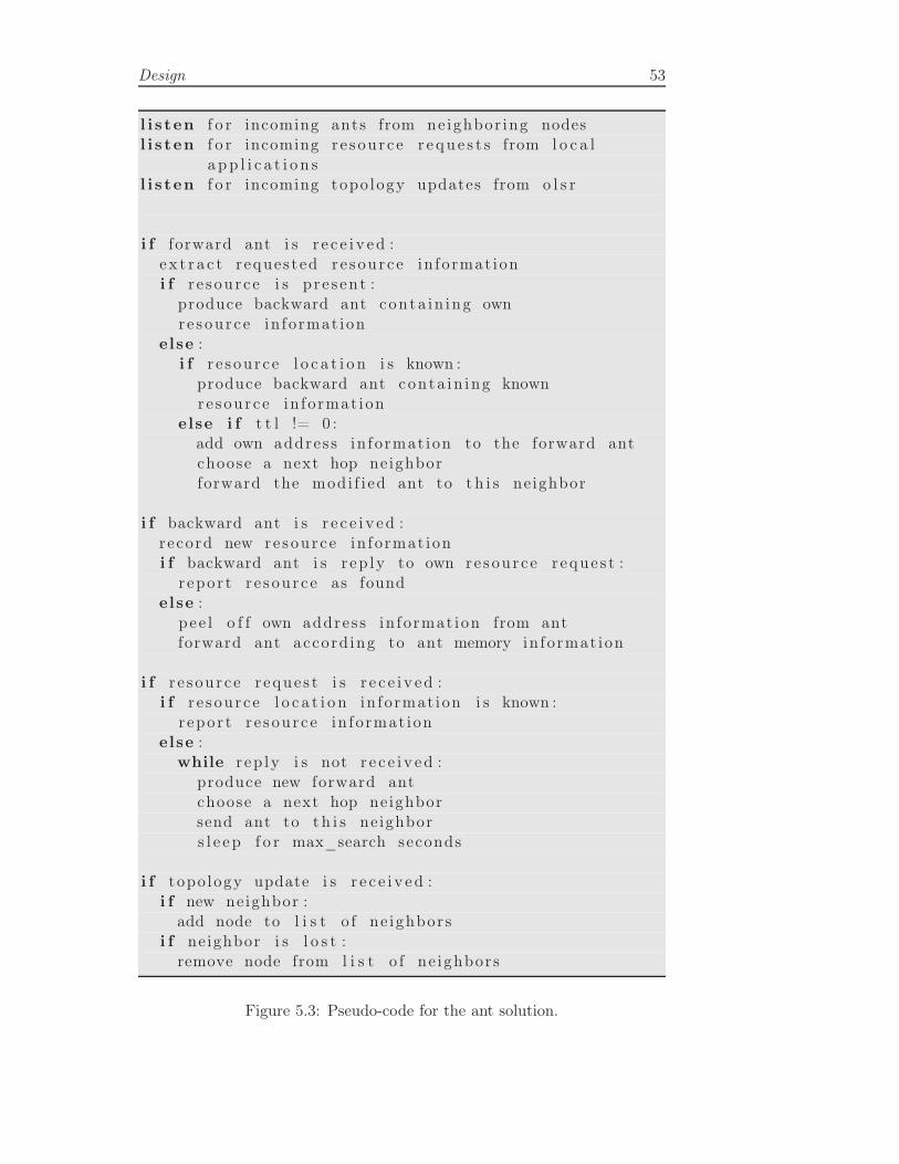
Design 53
l i s ten f o r incoming ants from ne ighbor ing nodesl i s ten f o r incoming re source r eque s t s from l o c a l
a pp l i c a t i o n sl i s ten f o r incoming topo logy updates from o l s r
i f forward ant i s r e c e i v ed :e x t r a c t reques ted re source in format ioni f r e s ource i s p r e s ent :
produce backward ant conta in ing ownre source in format ion
else :i f r e s ource l o c a t i o n i s known :
produce backward ant conta in ing knownre source in format ion
else i f t t l != 0 :add own addres s in format ion to the forward antchoose a next hop neighborforward the modi f i ed ant to t h i s neighbor
i f backward ant i s r e c e i v ed :record new re source in format ioni f backward ant i s r ep ly to own re source r eques t :
r epor t r e s ource as foundelse :
p ee l o f f own addres s in format ion from antforward ant accord ing to ant memory in format ion
i f r e s ource r eques t i s r e c e i v ed :i f r e s ource l o c a t i o n in format ion i s known :
r epor t r e s ource in format ionelse :
while r ep ly i s not r e c e i v ed :produce new forward antchoose a next hop neighborsend ant to t h i s neighbors l e ep f o r max_search seconds
i f topo logy update i s r e c e i v ed :i f new neighbor :
add node to l i s t o f ne ighborsi f neighbor i s l o s t :
remove node from l i s t o f ne ighbors
Figure 5.3: Pseudo-code for the ant solution.

Chapter 6
Implementation
”Vision without implementation is hallucination”
— Benjamin Franklin
In this chapter, we will explain the implementation of the design derivedin Chapter 5. The focus will be on the same parts of the program as thoseexplained in the design. As C code tends to get long even when doing quitesimple things, we will not show the complete code for the program, but rathercode snippets when appropriate. Some of the most important functions arelisted in Appendix D.
The first sections address some general issues such as choice of program-ming language and emulator-specific adaptations, before we move on to themore specific parts of the program and the various data structures used inSections 6.6 through 6.11. Finally, Section 6.12 provides an overview of theprogram flow and gives program execution instructions.
6.1 Remarks
This implementation is regarded as a prototype only. Our focus has been onthe ant principles rather than the code itself. It should thus be noted thatquite a few simplifications have been made during the implementation. Atseveral stages other, more elegant or resource utilizing approaches probablyexist. These considerations have, however, been left to a later stage, if thesolution turns out feasible for its purposes.
Also, even if this application is meant to run within a MANET, the codeis not written with this particularly in mind. Thus, in a production imple-mentation, changes should be made to the code to make it more suitablefor MANETs and their characteristics. For instance, messages sent over thewireless link should utilize tailored data types to use as little bandwidth as

56 Chapter 6
possible. Also, one might want to tailor other data structures and computa-tions to use as little computing resources as possible.
6.2 Programming Language
We have chosen to implement the prototype using the C [16] language. C is aquite small and quite low level, general-purpose programming language [21].C is not tied to any specific hardware or system, which makes C code highlyportable. In addition to this, C provides low-level memory access as wellas easy but powerful socket and networking facilities, making it especiallysuitable for our solution.
Also, we are going to do our testing with the NEMAN emulator. Whenrunning emulations, using a lightweight language such as C may be preferredover other, more heavyweight languages such as Java, which requires a virtualmachine and thus needs more computing resources per virtual node, as thisenables us to run tests with more nodes on one single computer.
6.3 Developing for NEMAN
Emulating in general and with NEMAN specifically will be explained inChapter 7. We do already state, however, that emulator testing requiresvery little program code adjustments. The only required adjustment in ourcode is that for the application to be able to listen and send messages onlyon a specified virtual device, the application, or more specifically an appli-cation’s sockets, need to be bound to this particular virtual device using theSO_BINDTODEVICE option. This is needed because all virtual devicesare running on the same machine.
More specifically, this is done in our code by calling the functionbind_socket_to_device() with a socket descriptor as argument. This func-tion is shown in Figure 6.1.
When using NEMAN, a message sent via one node to another might bedelivered up to the application layer at the intermediate node, even thoughit was not actually destined for this node. This behavior is normally notseen in real life, but to make everything work with NEMAN, we includeinformation about the actual destination in all messages to make sure noone handles messages meant for other nodes.
6.4 The sockaddr_in structure
The struct sockaddr_in is a builtin C structure that is heavily used in ourimplementation. This structure is used to address remote endpoints, and itis the structure used with the sendto() and recvfrom() system calls used inour implementation for sending and receiving messages, respectively.

Implementation 57
int bind_socket_to_device ( int sock fd ){
int rv ;i f ( ( rv = se t sockopt ( sockfd ,
SOL_SOCKET,SO_BINDTODEVICE,i f a c e ,s t r l e n ( i f a c e )+1)) == −1)
{write_log_error ( " so_bindtodevice " ) ;
}return rv ;
}
Figure 6.1: C code for binding a socket to a specific device.
struct sockaddr_in {short s in_family ;unsigned short s in_port ;struct in_addr sin_addr ;char s in_zero [ 8 ] ;
} ;
Figure 6.2: sockaddr_in C structure.
The contents of this structure is shown in Figure 6.2. The fields sin_portand sin_addr hold the port number and IPv4 address of the remote noderespectively.
6.5 Logging
To maintain a certain structure on the program output, we have chosento keep two kinds of logs: One for debugging purposes and one for systemtracking. The debug log is used to ease debugging, and is written to wheneversomething unexpected happens within the system. To ease error searching,we keep only one ”global” file. Obviously, this file will only be global if alldevices are actually running on the same machine, as is the case when testingwith NEMAN. If not, this file will also be local, as the path of the file willbe local to the machine the program instance is running on. In either case,each line in this file starts with the name of the node reporting the error.This file is called <program name>.debug, e.g. ant.debug.
For system tracking we keep one log per node. These files contain infor-
58 Chapter 6
mation on what has happened on each node, e.g. what forward and backwardants have been received, where they have been forwarded and what resourcelocations have been learned. These files are called <interface name>.log,e.g. tap1.log.
When running tests, some additional information is needed. When run-ning Make with the target test, an additional file, ant_test.log, is made. Allnodes write to this file whenever a request for a present resource is received.
6.6 Neighbor Information
6.6.1 Topology Information Retrieval
Neighbor information is retrieved from the OLSR daemon running on eachdevice. More specifically, this is done by establishing a TCP connectionto localhost on port 1212, which is listened to by OLSR. After connect-ing, OLSR will report any topology changes to port number 3458. OLSRmessages are on the following form:
<new/old route>,<to IP>,<via IP>,<no. hops>,<from device>
For example, the following message:
1,10.0.0.2,10.0.0.2,1,tap1
means that there is a new route from node tap1 to the node with IP address10.0.0.2 via the node with IP address 10.0.0.2. This route is one hop long,which means that 10.0.0.2 is a neighbor of tap1.
If the message starts with a 0, this means that an old route is lost. Thefollowing message:
0,10.0.0.2,10.0.0.2,1,tap1
means that the old route between tap1 and 10.0.0.2 is lost.
However, if a neighbor moves out of range, but there still exists an al-ternative path via other nodes to this node, OLSR will report this as a newroute, not a lost route:
1,10.0.0.2,10.0.0.3,4,tap1
In this example, there is still a route from tap1 to 10.0.0.2, but the newroute goes via 10.0.0.3, and is 4 hops long. Thus, if a new route message isreceived but the number of hops to this node is more than one, this nodeshould be removed from the list of neighbors (if present).
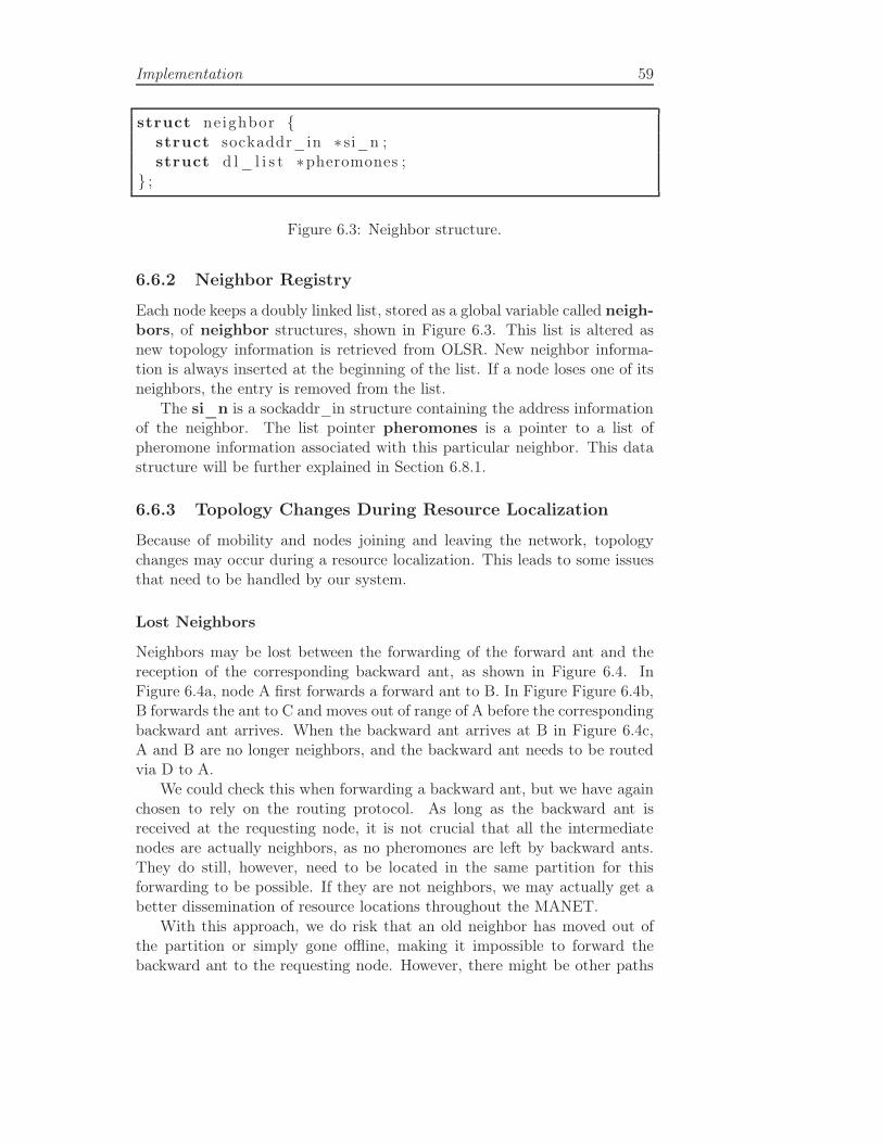
Implementation 59
struct neighbor {struct sockaddr_in ∗ si_n ;struct d l_ l i s t ∗pheromones ;
} ;
Figure 6.3: Neighbor structure.
6.6.2 Neighbor Registry
Each node keeps a doubly linked list, stored as a global variable called neigh-bors, of neighbor structures, shown in Figure 6.3. This list is altered asnew topology information is retrieved from OLSR. New neighbor informa-tion is always inserted at the beginning of the list. If a node loses one of itsneighbors, the entry is removed from the list.
The si_n is a sockaddr_in structure containing the address informationof the neighbor. The list pointer pheromones is a pointer to a list ofpheromone information associated with this particular neighbor. This datastructure will be further explained in Section 6.8.1.
6.6.3 Topology Changes During Resource Localization
Because of mobility and nodes joining and leaving the network, topologychanges may occur during a resource localization. This leads to some issuesthat need to be handled by our system.
Lost Neighbors
Neighbors may be lost between the forwarding of the forward ant and thereception of the corresponding backward ant, as shown in Figure 6.4. InFigure 6.4a, node A first forwards a forward ant to B. In Figure Figure 6.4b,B forwards the ant to C and moves out of range of A before the correspondingbackward ant arrives. When the backward ant arrives at B in Figure 6.4c,A and B are no longer neighbors, and the backward ant needs to be routedvia D to A.
We could check this when forwarding a backward ant, but we have againchosen to rely on the routing protocol. As long as the backward ant isreceived at the requesting node, it is not crucial that all the intermediatenodes are actually neighbors, as no pheromones are left by backward ants.They do still, however, need to be located in the same partition for thisforwarding to be possible. If they are not neighbors, we may actually get abetter dissemination of resource locations throughout the MANET.
With this approach, we do risk that an old neighbor has moved out ofthe partition or simply gone offline, making it impossible to forward thebackward ant to the requesting node. However, there might be other paths

60 Chapter 6
AB C
D
(a) Forward antmoves from A to B.
AC
D
B
(b) Forward antmoves from B toC, B moves outsiderange of A but intorange of D.
AC
D
B
(c) Backward ant hasto travel via D backto A.
Figure 6.4: Neighbor is lost between forwarding of forward ant and receptionof corresponding backward ant. Arrows show where the ants are moving.
neighbor
physically
lost
neighbor
chosen
as next
hop
topology
update
received
time
Figure 6.5: Neighbor is chosen as next hop before topology update is receivedby the ant application.
to this node. Thus, it might be a good idea to, in addition to the backwardant, send a request reply directly from the resource-holding node to therequesting node, increasing the possibility that the requesting node actuallygets a reply. This would introduce a slight overhead, but might be worth itif the node mobility is high enough. However, this has been left as furtherwork.
Delayed Topology Updates
Topology updates are delivered over a TCP connection from the OLSR dae-mon. There will always be a slight delay from the actual topology changeoccurs to the topology update information is delivered from OLSR to theant application. Information on new routes only makes the new neighborimpossible to select as a next hop until the topology update is received, andshould thus not cause any problems. Delayed route loss updates, however,make it possible to choose as next hop a node that is no longer a neighbor,as shown in Figure 6.5.
The chances of choosing a lost next hop neighbor during this very shortinterval is of course very small, but it might still happen and should thus behandled. However, as we are depending on the underlying routing protocol,a message sent to a lost neighbor should be received at this node as longas there is an alternative route to this node. Only if the node is completelyoutside the partition will the ant not be delivered there. This will make
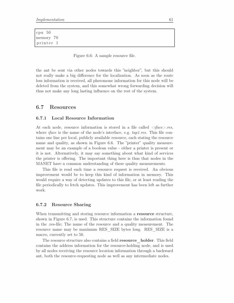
Implementation 61
cpu 50memory 70p r i n t e r 1
Figure 6.6: A sample resource file.
the ant be sent via other nodes towards this ”neighbor”, but this shouldnot really make a big difference for the localization. As soon as the routeloss information is received, all pheromone information for this node will bedeleted from the system, and this somewhat wrong forwarding decision willthus not make any long lasting influence on the rest of the system.
6.7 Resources
6.7.1 Local Resource Information
At each node, resource information is stored in a file called <iface>.res,where iface is the name of the node’s interface, e.g. tap1.res. This file con-tains one line per local, publicly available resource, each stating the resourcename and quality, as shown in Figure 6.6. The ”printer” quality measure-ment may be an example of a boolean value - either a printer is present orit is not. Alternatively, it may say something about what kind of servicesthe printer is offering. The important thing here is thus that nodes in theMANET have a common understanding of these quality measurements.
This file is read each time a resource request is received. An obviousimprovement would be to keep this kind of information in memory. Thiswould require a way of detecting updates to this file, or at least reading thefile periodically to fetch updates. This improvement has been left as furtherwork.
6.7.2 Resource Sharing
When transmitting and storing resource information a resource structure,shown in Figure 6.7, is used. This structure contains the information foundin the .res-file; The name of the resource and a quality measurement. Theresource name may be maximum RES_SIZE bytes long. RES_SIZE is amacro, currently set to 50.
The resource structure also contains a field resource_holder. This fieldcontains the address information for the resource-holding node, and is usedby all nodes receiving the resource location information through a backwardant, both the resource-requesting node as well as any intermediate nodes.

62 Chapter 6
struct r e s ource {char name [RES_SIZE ] ;int qua l i t y ;struct sockaddr_in resource_holder ;
} ;
Figure 6.7: Resource structure.
struct r e s ource_in f o {struct r e s ource r e source ;time_t expiry_time ;
} ;
Figure 6.8: Resource info structure.
6.7.3 Resource Location Info
Gathered resource location information is stored in resource_info struc-tures, as shown in Figure 6.8. Each node keeps a doubly linked list,known_best_resources, containing all gathered resource location infor-mation. A resource info structure contains a resource structure, as explainedin section 6.7.2, as well as an expiry time.
The expiry_time entry tells how long the snooped resource informationis valid, and should be adjusted according to the network characteristics. Atthe time, this value is equal for all nodes. Alternatively, it might be set bythe node holding the resource.
At the time, only the best known resources are stored, meaning that weonly store one location per resource name. This eases resource knowledgelookup and minimizes the storage needed. If a new resource is found, itsquality is compared to the quality of any previously found resource with thesame name. If the quality is better, the old entry is replaced with the new.If not, the new resource location is not recorded.
Unfortunately, for simplicity, entries are only removed from this list ifthe node receives a forward ant looking for the resource and the entry hasexpired. There is no automatic removal upon expiry. This may lead to verylong lists and makes the solution less scalable, but for the networks it issupposed to handle, it should work fairly good. This could be handled by a”garbage collector” thread that periodically ran through the list and removedexpired entries. However, this has been left as further work.
Implementation 63
6.8 Pheromone Traces
6.8.1 Pheromone Data Structure
Pheromone traces are recorded for each {neighbor, resource} couple. In otherwords, we need to store information for each resource and each neighbor. Tobe able to do this, we need to record all possible resources. As all possibleresources are not known, we restrict ourselves to all resources ever heard ofby the node. In addition to the list of known best resources, each node keepsa list all_known_resources, containing all resources the node has everheard about. Unlike the list of best resources, this list is add only — thereis no expiry time and no entries are ever removed from this list.
The easiest approach, which is also used by many other ant systems,would be to use a two-dimensional array with neighbors along one dimensionand resources along the other. However, both the number of neighbors andthe number of resources which someone will look for are unknown, makingit harder to declare a suitable array, although possible with dynamicallyallocated arrays. Also, there is no obvious mapping from resource namesand node identifiers to array indices.
Another possibility is to use ”two-dimensional linked lists”. This ap-proach, however, introduces a lot of redundancy and would require a lot ofwork to update.
Better solutions are possible, for example to use some kind of hash map,where the keys would be the {neighbor, resource} couple and the valueswould be the pheromone values. Although independent C libraries for hash-ing are available, we have chosen to use the list approach, as this introducedless implementation issues.
When using the two-dimensional list approach, we need to decide whatinformation should be stored on which list dimension. If the first level list isthe neighbors and the second level is one resource list per neighbor, we onlyhave to register each neighbor once, which is good. Adding and removingneighbors from this list is easy and cheap. Resources don’t need to be re-moved from the lists, so we only need to add these, even though they wouldneed to be added to every single neighbor when they first appear. How-ever, summarizing elapsed times for each neighbor for each resource, whichis needed when choosing the next hop for a forward ant, would in the worstcase require looping over the entire list structure.
On the other hand, if the first level list is a list of all resources, we haveto register all neighbors for all resources. As neighbors might come and go,this might require us to update each of these lists quite frequently, bothadding and deleting entries. Summarizing would be a lot easier, however, aswe only need to loop through the list of neighbors for the requested resourceand sum these, thus we only need to loop through one list, not the entiretwo-dimensional data structure.

64 Chapter 6
N1 N2 Nn
R1
R2
Rm
...
...
R1
R2
Rm
...
R1
R2
Rm
...
...
...
...
...
Figure 6.9: Two-dimensional linked list structure. First level list consists ofn neighbors, second level list consists of m resources.
struct pheromone {struct r e s ource ∗ r e s ource ;time_t last_used ;
} ;
Figure 6.10: Pheromone structure.
Which approach to choose depends on the usage. What happens mostfrequently: Neighbor updates or resource requests? If nodes move arounda lot, this implies a large amount of updates to the neighbor lists, and itwill thus be good to keep only one neighbor list. If resource requests aremore frequent, however, it will be more beneficial to keep only one resourcelist. For this system, neighbor updates will probably occur more frequentlythan resource requests. Thus, we have chosen the former approach. Theprinciples of the data structure is shown in Figure 6.9.
As the first level list is the list of neighbors, we may use the existing list ofneighbors also for pheromone value storage. As explained in Section 6.6.2,each neighbor structure includes a pointer to a list of pheromones. Morespecifically, this is a pointer to a list of pheromone structures, as shown inFigure 6.10.
This structure keeps a pointer to the corresponding entry in the

Implementation 65
all_known_resources list and the actual ”pheromone”: A timestampshowing when this neighbor was last used to look for this particular resource.
6.8.2 Pheromone Initialization
Whenever a new neighbor is discovered, it is added to the list of neighborsand a new pheromone list is created and added to the neighbor data struc-ture. The pheromone list contains all the resources from theall_known_resources list. The last_used entry is initialized to the boottime of the application on this node, giving all neighbors the same probabil-ity of being chosen if none are previously used, and a higher probability ofchoosing unused neighbors than previously used neighbors if some are usedand some are unused.
Whenever a node receives a resource request for a resource that is notstored in the all_known_resources list, it is added to this list and to allexisting neighbor-pheromone lists. The last_used entry is again initializedto the application boot time.
6.8.3 Pheromone Updates
Whenever a node is used as next hop to search for a given resource, thecorresponding {neighbor, resource} last_used entry is set to the time ofusage.
At the time, if a neighbor is lost, the entire neighbor and its associatedpheromone list is deleted. It might perhaps be a good idea to keep theselists, at least for a little while, in case the neighbor moves back into range.In systems with high mobility, nodes may move in and out of range of eachother quite frequently, and thus cause frequent building of new pheromonelists, as well as re-initializing all timestamps associated with each {neighbor,resource pair}.
6.9 Ants and Ant Memory
Both forward as well as backward ants consist of an ant structure followed bya number of struct sockaddr_in structures. These structures were chosento ease the forwarding of backward ants, as these may be used unchanged incalls to sendto(), the function used for sending messages. The address infor-mation is added by the receiving node, not the sending node. There are twoadvantages with this approach: The ant size is increased one step later intothe procedure, putting less load on the network, and the address informationis easily available as this is returned by the call to recvfrom(). The C structused for ants is shown in Figure 6.11. The type field must be either ’F’, forforward ants, or ’B’, for backward ants. preceding_ants is the number ofants that have previously been sent to look for the same resource. This is
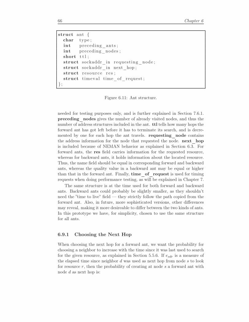
66 Chapter 6
struct ant {char type ;int preceding_ants ;int preceding_nodes ;short t t l ;struct sockaddr_in request ing_node ;struct sockaddr_in next_hop ;struct r e s ource r e s ;struct t imeva l time_of_request ;
} ;
Figure 6.11: Ant structure.
needed for testing purposes only, and is further explained in Section 7.6.1.preceding_nodes gives the number of already visited nodes, and thus thenumber of address structures included in the ant. ttl tells how many hops theforward ant has got left before it has to terminate its search, and is decre-mented by one for each hop the ant travels. requesting_node containsthe address information for the node that requested the node. next_hopis included because of NEMAN behavior as explained in Section 6.3. Forforward ants, the res field carries information for the requested resource,whereas for backward ants, it holds information about the located resource.Thus, the name field should be equal in corresponding forward and backwardants, whereas the quality value in a backward ant may be equal or higherthan that in the forward ant. Finally, time_of_request is used for timingrequests when doing performance testing, as will be explained in Chapter 7.
The same structure is at the time used for both forward and backwardants. Backward ants could probably be slightly smaller, as they shouldn’tneed the ”time to live” field — they strictly follow the path copied from theforward ant. Also, in future, more sophisticated versions, other differencesmay reveal, making it more desireable to differ between the two kinds of ants.In this prototype we have, for simplicity, chosen to use the same structurefor all ants.
6.9.1 Choosing the Next Hop
When choosing the next hop for a forward ant, we want the probability forchoosing a neighbor to increase with the time since it was last used to searchfor the given resource, as explained in Section 5.5.6. If esdr is a measure ofthe elapsed time since neighbor d was used as next hop from node s to lookfor resource r, then the probability of creating at node s a forward ant withnode d as next hop is:

Implementation 67
struct neighbor_prob {struct neighbor ∗neighbor ;struct pheromone ∗pheromone ;
} ;
Figure 6.12: Neighbor_prob structure.
psdr =
{
esdrPn
i=0esir
, if d ∈ Ns,
0, if d /∈ Ns
where Ns is the set of neighbors of node s, excluding the forward ant’s lastpredecessor.
The actual choosing is implemented by generating a random numberin the interval [0, 1]. Let’s say we have a list of all neighbors and theirassociated probabilities for the given resource, and a variable sum. Then weloop through the list of neighbors, and for each neighbor add the probabilityassociated with the neighbor to sum. Then, we check if sum is less thanor equal to the random number. If it is, we choose this neighbor, if not, weproceed to the next neighbor in the list.
To do this, we use the pheromone data structure explained in section6.8.1. This structure contains the time of last use for each {neighbor, re-source} pair available. Because of the choice of primary (neighbor) andsecondary (resource) lists in this two-dimensional list structure, this endedup getting a bit more ugly that we had hoped: To find all available neigh-bors and the associated time of last use for the requested resource, we haveto loop through the entire two-dimensional list structure. To avoid loop-ing over this entire structure more than once, we build a new temporarystructure containing only the appropriate {neighbor, resource} pairs, wherethe appropriate pairs are those with same resource name and quality. Theappropriate pairs are stored in a list of neighbor_prob structures, eachrepresenting a neighbor-resource pair. This structure is shown in Figure6.12. The temporary list is deleted when the next hop has been chosen.
The entire pheromone struct is included instead of just the resource, asthe time of last usage, which is stored in the pheromone structure, needs tobe updated if the neighbor is chosen.
When building the list of appropriate {neighbor, resource} couples, thelast hop neighbor from which the ant arrived is skipped, and thus not addedto the list of available neighbors. This is done to avoid sending the requestback to this node. However, if the list of available nodes is empty after thisphase, meaning that this last hop node is the only neighbor, the request issent back to this node. The alternative would be throwing the ant away, butby doing this, we allow the ant to try another path instead.

68 Chapter 6
A
B
C D
E
B B - C - D
A - B - E - B - C - D
A - B - C - D
source node
scanning direction
scanning for node B
first occurrence of B
from destination node
Final path
...
Figure 6.13: Loop elimination in backward ants.
6.9.2 Loop Elimination
As backward ants should not travel in loops, all loops are removed from thebackward ant before it is sent from the resource-holding node. This is doneby looping through the list of visited nodes starting at the source node, andfor each node, a reversed search through the same list is used to look forequal entries. If one is found, every node in between is removed from thelist. The fundamentals of the approach are shown in Figure 6.13. In thisfigure, the forward ant has visited node B twice. During loop elimination,the loop, i.e. nodes B and node E, is removed from the list of visited nodes.
This approach also works if the same node is visited more than twice, asthe occurrences in between first and last visit are removed the first time aloop is discovered.
The number of preceding nodes is updated correspondingly to matchthe length of the path that the backward ant is going to walk back to therequesting node.
6.9.3 Ant Communication
All nodes are listening for incoming ants on port 3456.
6.10 Resource Localization
In this section, we will explain how a resource localization is initiated andterminated.
6.10.1 Search Initiation
All nodes listen for incoming resource requests. Resource requests are sentto a node via UDP segments to port 3457. Resource requests contain in-formation about the resource, and should be on the form ”<resource name><minimum quality>”. We do not check that resource requests are sent fromthe same device as the one that received the request, thus, anyone may senda request for a resource to any node, provided there is a path from the actualrequesting node. The result, however, is only written to file on the node thatreceived the request.

Implementation 69
Before a forward ant is produced and sent, we check if a suitable resourcelocalization is already known and listed in known_best_resources. If itis, it is not necessary to do a search. This check is performed again everytime a new forward ant is about to be sent, as new resource information mayhave been snooped since the last ant was sent max_sleep_time secondsago.
When a search is initiated, the requested resource is added to a list ofongoing searches, not_found_resources.
6.10.2 Search Termination
A search is terminated when the requested resource is found. While theresource is not located, a new search for the same resource is initiated everymax_sleep_time seconds, a value which is provided by the user uponstartup. Currently, there is no possibility to terminate the search in anyother way.
When a backward ant arrives at the requesting node having found aproper resource, the resource is removed from the list of ongoing searches.When doing this, all nodes satisfied by the localized resource is removed.
After max_sleep_time seconds, we check if the list of ongoing searchesstill includes the requested resource. If it does, the resource was not found,and we initiate a new search. If not, the resource was found and the searchis terminated.
When a backward ant arrives at the resource-requesting node, the re-quested resource is removed from not_found_resources. After each se-arch has had max_sleep_time seconds to terminate, we check if the re-source is still listed in not_found_resources. If it is, the resource is notyet found, and a new search is initiated. If it has been removed from the list,this means that the resource has been localized, and the search is terminated.
6.11 Utilities
As most of the data structures are doubly linked lists, we have made a”generic” doubly linked list implementation used to handle all these lists.The structure for the lists is shown in Figure 6.14.
Each list element is thus of this data type. The void pointer entry isa pointer to the actual entry. This may for example be a neighbor structor a resource struct. This approach introduces an extra step to access theactual information stored in the list, but makes it possible to use the samefunctions for adding and deleting entries in lists of any data type.
Along with the structure, we have implemented functions for inserting anelement at the beginning of the list, deleting a specified element and deleting(with freeing of memory) an entire list.

70 Chapter 6
struct d l_ l i s t {struct d l_ l i s t ∗prev ;struct d l_ l i s t ∗next ;void ∗ entry ;
} ;
Figure 6.14: Doubly linked list structure.
6.12 Program Flow
6.12.1 Threads
As the program should be able to manage several tasks at once, it is dividedinto several threads:
• The main process: Listens for incoming ants, forward as well as back-ward.
• Thread 1: Listens for incoming topology updates and handles the listof neighbors. Created by the main process shortly after startup.
• Thread 2: Listens for incoming resource requests. Created by the mainprocess shortly after startup.
• Thread 3: Initiates a new search every max_sleep_time seconds. Cre-ated by Thread 2 for every incoming resource request.
• Thread 4 and 5: Handles backward and forward ants, respectively.Created by the main process whenever receiving an ant.

Chapter 7
Test Setup
”Experience is the worst teacher. It always gives the test first
and the instruction afterward.”
— Source unknown
In this chapter we explain the setup used during our tests, includingexplanations of the tools used, the network scenarios in which the tests areperformed as well as the setup of the actual experiments done.
When performing a performance analysis, several choices must be made:Which evaluation technique to use, which environment to perform tests inand which metrics to evaluate the system on. This chapter gives a gen-eral overview of some of the available techniques and tools, as well as anexplanation of the specific tests used to analyze our system.
When testing our resource localization solution, we need to perform teststhat reflect the goal and requirements for our solution, stated in Chapter 5.The tests should verify that the goals for the solution are reached, thus thatnodes looking for a resource are able to locate this resource if it is presentin the MANET. We also test how well the solution performs with regard tothe requirements stated in Section 5.3, thus how well the solution utilizesthe resources present in the network, both in terms of networking resourcesand local processing power at each node. We also take a look at how fastthe solution is able to localize a given resource. An explanation of how ourtests are set up and performed in provided in Sections 7.5 through 7.9.
In Section 7.4, we present an alternative to the ant solution, used to getcomparable results for our analysis.
7.1 Evaluation Techniques
Evaluation techniques may be split into three different approaches [17]:

72 Chapter 7
• Analytical modeling: Involves mathematical models and formal proofs,and requires simplifications and assumptions to make usable models.Gives quite low accuracy, but requires relatively little time, given thatyou are trained in making such models, and also does not require thesystem to actually exist when ”testing”.
• Simulation: The system is tested within a controlled and, probably,somewhat simplified environment. This gives a higher accuracy thanmodeling, but requires more time and resources to perform. One maytest only parts of the system, making it possible to perform tests beforea complete running system is made.
• Measurements: Measurements means doing real-world testing, i.e. totest the system in its natural environment. Performing measurementsrequires the system in question to actually exist and be ready for fulltesting. Measurements also require a full testing environment, resultingin a high cost and low repeatability. However, as the system is testedin the environment it is supposed to run in, this technique may givevery reliable and accurate results. However, environmental parameterssuch as system configuration, workload and time of the measurementmay affect the results. The accuracy may thus vary between none andhigh [17].
Analytical modeling requires substantial knowledge in areas like math-ematics and queuing theory, as well as the time to develop good models.This, along with the potentially low level of accuracy, makes this techniqueunsuitable for our testing. As real-world measurements require a lot of timeand resources and provides low repeatability, also this solution is ratherunsuitable for our purposes. Simulation, on the other hand, both gives mod-erate accuracy and takes relatively short time to perform, and is thus theevaluation technique chosen to perform our testing.
The techniques listed above may also be used in combination. For ex-ample, one might use analytical modeling together with simulation to verifyand validate the results obtained from each technique. In [17, p. 32], Jainstates the three rules of validation:
• ”Do not trust the results of a simulation model until they have beenvalidated by analytical modeling or measurements.”
• ”Do not trust the results of an analytical model until they have beenvalidated by a simulation model or measurements.”
• ”Do not trust the results of a measurement until they have been vali-dated by simulation or analytical modeling.”
According to these rules, we should thus not rely only on the results fromour simulations, but have them validated by either analytical modeling or

Test Setup 73
real-world measurements. However, this has, because of time issues, beenleft as further work.
7.2 Testing Environment
7.2.1 Simulation vs Emulation
Above, we used the word ”simulation” for testing a system within a con-trolled and simplified environment. However, this kind of ”simulation” maybe further divided into simulation and emulation. One goal of simulators,such as GloMoSim [43] and ns-2 [40], is to give a detailed representationof the physical layer [31]. Simulators are suitable for large-scale networks,and provide reproducible results [30]. However, code written for a simula-tor needs to be rewritten before it can be used on a real platform. Also,simulators take a substantial amount of time to learn to use and program.
In emulators, such as NEMAN [31] and MobiNet [22], parts of the pro-tocol stack may be simulated while the rest is the real implementation inquestion. This code requires very little adjustments to work on a real plat-form, possibly saving a lot of time during implementing. Like simulators,emulators produce reproducible results. However, emulators tend to pro-vide less scalability than simulators, although this depends on the emulatorimplementation.
7.2.2 ns-2
ns-2 [40] is a network simulator which for a long time has been used toperform simulations in the ad-hoc network research area. When using ns-2, the user specifies a network topology and the movement patterns of thenodes within this topology, called a scenario. The scenario file provides adetailed description of all the nodes in the network and their behavior duringthe emulation, for example their start position, their distance to all othernodes in the network and in which direction they are moving at what speedat different times during the emulation. The simulator is able to ”play”this scenario, enabling the user to perform measurements and analyses ofimplemented applications without having to set up a real life test scenario,which may be a costly and highly time consuming operation.
7.2.3 NEMAN
NEMAN is a network emulator. Because of the availability of researcherswith high expertise on NEMAN within the research group, we have chosento use NEMAN to perform the performance analysis for this thesis.
For NEMAN to be able to emulate a given network topology, this topol-ogy needs to be specified in a scenario file, just like ns-2. NEMAN uses

74 Chapter 7
standard ns-2 scenario files, which enables us to use any available ns-2 sce-nario file generator to make scenario files for NEMAN. NEMAN scenariofiles also allow scenario files to define messages to be sent to specific nodesat certain times during the emulation. This may for example be used toactivate certain functionality within the applications.
NEMAN Components
NEMAN consists of three elements [31]:
• User processes: The applications and protocols that are to be tested.
• Topology manager: Manages virtual network interfaces and performspacket switching according to the topology information at a certainmoment in time.
• Graphical user interface: Provides a graphical interface to the emula-tor. Visualizes the emulated network, i.e. nodes, node ranges and nodemovement. Induces topology information to the topology manager.
The user processes hook to virtual Ethernet network devices called TAPdevices. These may be used together with the classical socket API, enablinguser processes to send and receive data. However, all user processes mustbind to a specific TAP device using the option SO_BINDTODEVICE toavoid interference with traffic addressed to other processes.
The virtual interface tap0 is reserved as monitoring channel. This inter-face has an open bidirectional connection to all other virtual interfaces, andthus hears all traffic in the emulated network.
7.2.4 OLSR daemon
The OLSR daemon olsrd [1] is an implementation of OLSR. olsrd supportsmesh routing for any network equipment with a wifi card with ad-hoc sup-port, as well as all ethernet devices. In our experiments, we have used olsrdversion 0.4.10.
7.3 Emulation and Analysis Tools
7.3.1 setdest
The scenario files needed by NEMAN and ns-2 may be created by hand, butthere also exists programs that, based on some simple parameters, createready-to-use scenario files for you. setdest [15] is an example of such aprogram.
setdest exists in two different versions, the original 1999 CMU version(version 1) and the modified 2003 U.Michigan version (version 2). For our

Test Setup 75
experiments, we will be using the original version. This version takes sevenparameters:
./setdest -v <1> -n <nodes> -p <pause time> -M <max speed>
-t <simulation time> -x <max X> -y <max Y>
This command creates a scenario consisting of nodes nodes, moving witha maximum speed of max speed meters/second for a time period of lengthsimulation time seconds, initially placed within the area defined by the maxX and max Y coordinates. setdest nodes move according to the randomwaypoint model (RWM) [18]. In RWM, nodes move between waypoints,which are uniformly distributed over the given area. Nodes may pause forup to pause time seconds at each waypoint.
7.3.2 tcpdump
tcpdump [2] is a tool for intercepting and displaying the network traffic ona specified network interface. The output from tcpdump is a description ofall captured packets. This description may, amongst other things, containinformation about source and destination of all packages, tcpdump uses thelibpcap library to capture all packets.
Running tcpdump with the -w flag produces a file containing all packetdata for later analysis. Our tests will be run with this option, enabling usto use other analysis tools on the data on a later stage.
7.4 A Flooding Solution
The results from the ant solution alone are not enough to say anything aboutthe quality of the solution. Thus, we need some other system to comparethe performance of the ant solution with.
As a comparative solution, we have implemented a simple flooding solu-tion. In this solution, instead of sending forward ants, a resource-requestingnode broadcasts a resource request. Each receiving node re-broadcasts therequest if the resource is not present. If the resource is present, a resourcereply is sent directly back to the requesting node.
7.4.1 Issues with Flooding
Flooding is a very efficient solution where one wants quick dissemination ofmessages into the network. In our case, we want to find a certain resourcethat might be located at some unknown node in the network. By flooding aresource request, all nodes in the network (partition) will get the request ina minimal number of hops, and if a resource-holding node exists, it will beable to reply quickly, thus minimizing the response time.

76 Chapter 7
However, there are also issues with flooding, especially within MANETs.In a MANET, communication is performed with the CSMA/CA scheme, asexplained in Section 2.1.2. In such a network, flooding comes with severaldrawbacks [24]. First of all, not only the resource-holding node receives therequest. So does also all other nodes in the entire network. In the mostbasic flooding approach, every node re-broadcasts every single request if theresource is not present at the node. As broadcast messages will go back andforth between neighboring nodes, this will lead to endless flooding, againleading to massive load on the network if the request is not at some pointstopped, for example after a given number of hops.
The same broadcast message will also be picked up by all neighbors atapproximately the same time. Those neighbors that do not hold the resourcewill decide to re-broadcast, again approximately at the same time. Chancesare, at least some of these neighbors are within range of each other. Their re-broadcasts will then most likely contend with each other. The re-broadcastmessages may also collide with each other.
A ”massive load” is not wanted in any network, and certainly not ina MANET. A lot of adjustments may be made to the basic flooding ap-proach to make it less resource demanding. An obvious improvement, whichaddresses the re-broadcasting problem mentioned above, is to only allow re-broadcasting of a certain message once at each node. To make this possible,some sort of message identification is needed, together with registration ofwhich messages have already been re-broadcast.
Other mechanisms are also available, such as the probabilistic scheme,counter-based scheme, distance-based scheme, location-based scheme andcluster-based scheme. Generally, these schemes use different techniques toreduce the number of redundant re-broadcasts, and thus also contention andcollision. For a review of these schemes, see [24].
7.4.2 Flooded Requests
A node looking for a resource broadcasts a request, currently to its one hopneighbors (IP address 10.0.255.255). All receiving nodes check if they havethe resource. If they do, they reply to the requesting node. If not, theyre-broadcast the request to all their one-hop neighbors.
In our simple flooding solution, we have used only one load-reducingtechnique, namely the one stopping nodes from re-broadcasting the sameresource request more than once. In the ant solution, we kept a maximumnumber of hops to keep requests from living ”forever” in case the requestedresource is not present within the network. In the flooding solution, however,these requests will be stopped by the former technique when all nodes havereceived the request once. Thus, such a time-to-live value is not used in theflooding solution.

Test Setup 77
7.5 Monitoring
A monitor is a tool that is used to observe the activities within a system.They observe system performance, collect performance statistics, analyzedata and display results, and may also identify problem areas and suggestremedies [17]. Monitoring is a key step in measuring system performance, asthis is the phase where all data is collected.
Monitors may be placed inside or ”outside” the system in question. Tobe able to place a monitor inside a system, we need to have access to andbe able to modify the system’s source code. This approach may give a veryhigh level of detail, but may also add additional overhead to the system inquestion, as the system is modified to make room for the monitor.
A monitor placed outside the system does (probably) not get the samelevel of detail, as the only data available to the monitor is the system inputand output. However, no additional overhead is added to the system inquestion, giving a high level of result correctness.
In our testing, we use both kinds of monitors: Response time monitor-ing is implemented in the source code, and is inside the system. Resourceutilization monitoring, however, is performed outside the system.
7.6 Metrics
To be able to measure the performance of our system, we must define a setof metrics. The metrics are the performance criteria that the system will betested upon.
The outcome of a system request may be one out of three [17]: Theservice is performed correctly, incorrectly or not performed at all. The metricsassociated with these three outcomes are speed, reliability and availability,respectively.
During our performance testing, we will only be concerned with the firstkind of outcomes, thus we assume correct performance at all times. Per-formance analysis of correctly performed tasks may be measured by thetime taken to perform the task (responsiveness), the rate at which the taskis performed (productivity) and the resource consumption while the task isperformed (utilization). These metrics are often referred to as response time,throughput and utilization, respectively. In this thesis, we will focus on theresponse time and the resource utilization achieved by our solution.
Metrics may be further divided into individual metrics, concerning theutilization experienced by one user only, or global, reflecting the utilizationexperienced by the system as a whole.
To get dependable results, experiments should be performed several times.The final result for one metric will then often be the mean value of the re-sults from all experiments. However, one should be aware of the variance
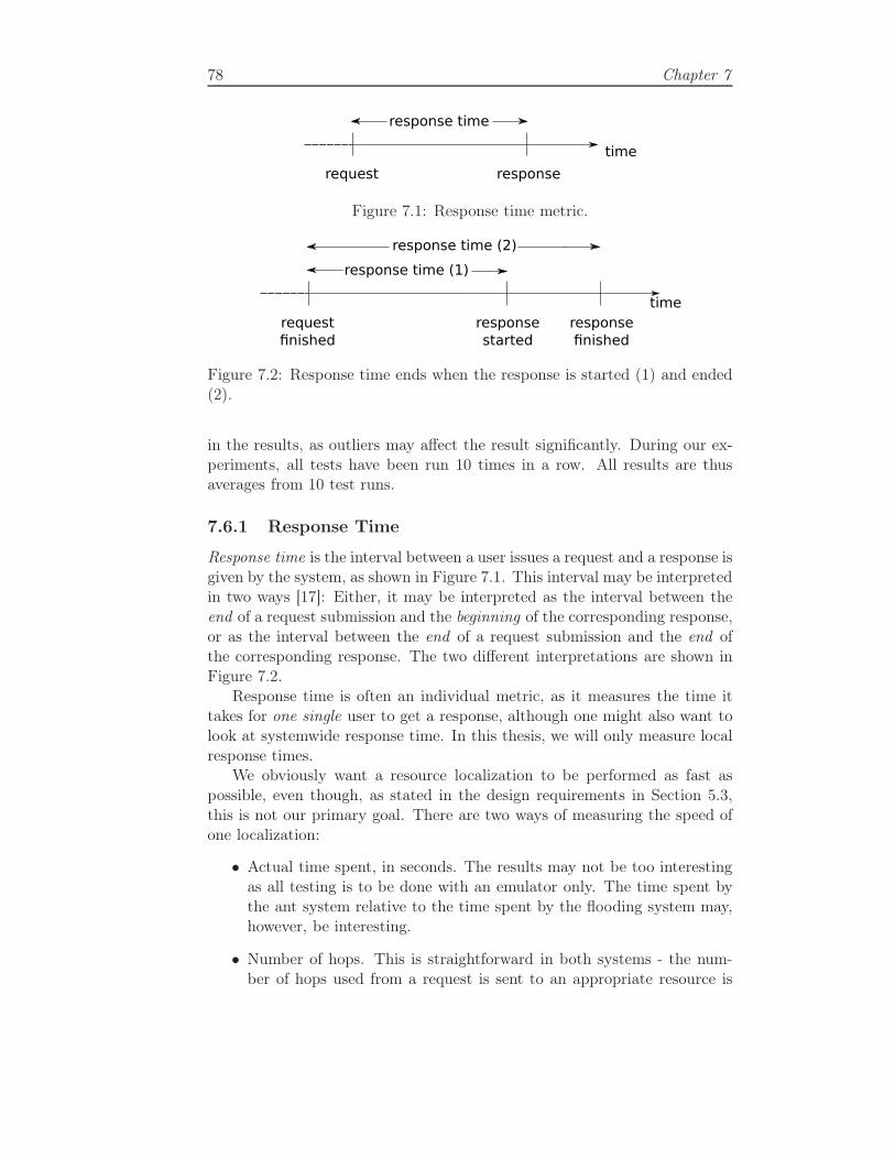
78 Chapter 7
response
time
request
response time
Figure 7.1: Response time metric.
time
request
finished
response time (1)
response
started
response
finished
response time (2)
Figure 7.2: Response time ends when the response is started (1) and ended(2).
in the results, as outliers may affect the result significantly. During our ex-periments, all tests have been run 10 times in a row. All results are thusaverages from 10 test runs.
7.6.1 Response Time
Response time is the interval between a user issues a request and a response isgiven by the system, as shown in Figure 7.1. This interval may be interpretedin two ways [17]: Either, it may be interpreted as the interval between theend of a request submission and the beginning of the corresponding response,or as the interval between the end of a request submission and the end ofthe corresponding response. The two different interpretations are shown inFigure 7.2.
Response time is often an individual metric, as it measures the time ittakes for one single user to get a response, although one might also want tolook at systemwide response time. In this thesis, we will only measure localresponse times.
We obviously want a resource localization to be performed as fast aspossible, even though, as stated in the design requirements in Section 5.3,this is not our primary goal. There are two ways of measuring the speed ofone localization:
• Actual time spent, in seconds. The results may not be too interestingas all testing is to be done with an emulator only. The time spent bythe ant system relative to the time spent by the flooding system may,however, be interesting.
• Number of hops. This is straightforward in both systems - the num-ber of hops used from a request is sent to an appropriate resource is

Test Setup 79
localized.
Measuring the Response Time
In the flooding approach, a resource reply is sent directly from the resourceholder to the requesting node. In the ant solution, however, the backwardant travels the whole search path back to the requesting node (excluding anyloops).
As mentioned above, there are two different definitions of response time,where the difference is where the response time measurement is stopped.When measuring the time spent on one resource localization, we thus needto define the term ”resource localization” - does this include the reply backto the requesting node? If the duration of the response is long, the preferreddefinition is the latter, where the duration of the system response is includedin the response time. If we use this definition, the ant solution may needtwice as many hops as if we excluded the reply. One might argue thatthese hops should be included, as it doesn’t help the requesting node muchthat some node out there knows the location of the resource - it needs thisinformation itself. However, there is an obvious possible improvement tothe ant solution here: The resource holder may, in addition to sending thebackward ant towards the source, also send a direct resource reply like inthe flooding system. This introduces a slight overhead, as the requestingnode will also receive the backward ant at a later point, but will improve theresponse time. This improvement is not implemented in our solution, butmakes it possible to exclude the reply from the hop count and use the firstdefinition - the response time is the interval from the forward ant is sent toit is received at a resource-holding node.
In the ant system, the requesting node sometimes needs to send morethan one forward ant. During testing, we assume each forward ant that doesnot produce a reply has reached the time to live-limit, and thus count timeto live hops times the number of non-returning ants plus the number of hopstraveled by the ant that actually found the resource. Also, the response timein number of seconds is measured from the first forward ant is sent to searchfor a given resource.
Logging
Requesting nodes log the time at which a request is received, righ before thefirst forward ant or resource request is sent. Each ant and flooded requestcontains a field keeping track of the number of preceding nodes, and forwardants also how many ants have already tried to localize the resource withoutreturning. Receiving resource holders log both the time of reception as wellas the number of hops the request (counting ttl hops for every non-returningforward ant) has traveled. All values are written to the global result log.

80 Chapter 7
7.6.2 Resource Usage and Utilization
The utilization of one resource is the fraction of time the resource is busyservicing requests [17]. As stated in the design requirements in Section 5.3,the main requirement for our solution is that a resource localization consumesas little resources, both local as well as network resources, as possible. Thus,we divide our resource usage measurements into two parts: Bandwidth usageand local processing power usage.
Bandwidth Usage
In general, the bandwidth usage should be measured from a search is startedto the requesting node receives a reply. As opposed to the response timemeasurements, when measuring the resource usage, the reply traffic maynot be omitted. Thus, for the ant system, the message count includes bothforward as well as backward ants. If a search is initialized and no replyis received within max_sleep_time seconds, a new forward ant should besent, and resource usage monitoring is continued until a reply is received. Itmight happen, however, that a new search is started before a backward antfrom a previous search reaches the requesting node. Thus, we need to keepmonitoring until there is no network activity.
The same holds for the flooding solution. The message count consistsof the number of broadcast messages plus the one message needed to replyto the requesting node. We cannot stop the monitoring when a reply isreceived, as the flooding might still be going on in other parts of the network— other nodes will not know that a resource is already localized. Thus, asin the ant solution, we need to keep monitoring until there is no activity inthe network.
Message Count To get a view of the bandwidth usage of the two systems,the number of messages sent in the entire network during one resource local-ization is measured. By measuring the number of sent messages, a broadcastmessage will count as one message, no matter how many nodes receive themessage.
The message count MCbw in a network of n nodes is thus:
MCbw =
n∑
i=1
(messages sent from n). (7.1)
Byte Count Counting the number of messages may give a good pictureof the resource usage of the two systems, but the resource usage dependsnot only of the number of messages sent, but also the size of the messages.Sending a few large messages might take just as much resources as sendingseveral smaller messages. Thus, we also measure the number of bytes sent

Test Setup 81
during resource localization. Comparing the number of bytes sent with thenumber of messages sent tells us if the message count is accurate enough, orif the size difference is large enough to affect the results of the two systems.
The byte count for bandwidth usage, BCbw in a network of n nodes isthus:
BCbw =
n∑
i=1
(bytes sent from n). (7.2)
Utilization In general, the message count alone is not enough to concludeon the bandwidth utilization. We need to know how many of the messagesthat were sent that were actually used for something.
In the ant system, all messages are either forwarded or replied to, exceptfor forward ants with ttl = 0. Thus, we expect almost full bandwidth utiliza-tion. In the flooding system, however, a sent message is regarded utilized,in bandwidth manner, if at least one of the recipients either re-broadcast itor answers to it. The utilization Ubw in a network with n nodes is thus:
Ubw =
∑ni=1(messages replied to at n)∑n
i=1(messages sent from n). (7.3)
However, the ant solution bandwidth utilization should be ≈ 1, as allreceived messages should be either answered to, if the resource is present,or forwarded, if the resource is not present. The only reason for this not tohappen is if the forward ant has a ttl = 0. In this case, the ant dies and thewhole search is wasted, not only the last jump. Thus, we have not conductedany measurements of the bandwidth utilization.
Local Processing Power Usage
The measured bandwidth usage provides information on the network load.However, one characteristic of wireless transmission is that all nodes withinrange of a transmitter will pick up the message and check if it is destinedfor itself. If it is, the resources used to handle this message were not wasted.However, if the message was not destined for this node and is thus thrownaway, this resource usage was a complete waste.
This characteristic is not very well exploited in the ant solution. Here,all messages are destined for one specific node. Thus, there is one recipient,so the message will not be wasted in terms of bandwidth, but all nodes thatpick up the message but find it to be destined for some other node, do wastesome processing power on this message handling.
In the flooding solution, on the other hand, this characteristic is exploitedand used to spread the request as fast throughout the network as possible.Still, a lot of messages that have already been re-broadcast may be receivedagain from other sources, and are thus wasted, as each node will only re-broadcast the same message once.

82 Chapter 7
There is a difference between wasted messages in the ant solution andwasted messages in the flooding solution, however. In the ant solution,wasted messages are thrown away at the network layer when the routingprotocol discovers that this message was not destined for this node. In theflooding solution, however, ”waste” is not discovered before the message is tothe application layer and the application finds out this message has alreadybeen re-broadcast, and thus waste even more resources than those in the antapplication. However, for simplicity, in our analysis, all wasted messages areregarded equal.
Message Count In this case, we count the number of received messages.Even if a message is broadcast and is thus only sent once from the source,every receiving node needs to handle the message.
The message count MClpp in a network if n nodes is thus:
MClpp =n∑
i=1
(messages received at n). (7.4)
Byte Count As in the bandwidth measurements, we also look at the num-ber of bytes sent by the two systems. The byte count for local processingpower usage, BClpp in a network of n nodes is:
BClpp =
n∑
i=1
(bytes received at n). (7.5)
Utilization As with bandwidth, we want to know how good the localprocessing power utilization is. The utilization is the fraction of messages orbytes that are actually ”used” to the total number of received messages orbytes. Thus, the utilization Ulpp in a network of n nodes is:
Ulpp =
∑ni=1(messages replied to at n)∑n
i=1(messages received at n), (7.6)
or alternatively
Ulpp =
∑ni=1(bytes replied to at n)∑n
i=1(bytes received at n). (7.7)
Topology Update Messages
In the ant system, we communicate with olsr to get topology information. Asthis is only communication between two ports on the same (virtual) node, itonly imposes local load on each node, not on the network, and these messagesare thus omitted from message and byte counts.

Test Setup 83
1n
Figure 7.3: Chain topology.
7.7 Test Scenarios
The test scenarios are the virtual environments in which the solutions aretested. The scenarios define the network topology and node mobility, as wellas the node behavior, meaning resource localization initialization.
For the tests to give as realistic results as possible, the node mobilityand behavior should be as close to that in real life usage of the system.The best is to use real world traces to define node mobility. However, realworld traces are not highly available, and are typically quite advanced. Inthis thesis we instead use only a few, quite basic scenarios to show and verifybasic functionality and the most important principles. One scenario includesnode mobility, but no node joins or leaves are included in any scenario.
7.7.1 Chain Scenario
The simplest possible topology is a static chain, as shown in Figure 7.3. Inthis scenario, every node has minimum one neighbor (the chain ends) andmaximum two neighbors (the middle nodes).
In this scenario, we expect both solutions to behave similarly until aresource is located, as the only possible path for the forward ant to travel isstraight through the chain, which should also be the path of the broadcastmessages.
7.7.2 Grid Scenario
In the grid scenario, in which we still use static nodes, the number of neigh-bors per node increases. The four corner nodes have two neighbors, otheredge nodes have three neighbors and the middle nodes have four neighbors,as shown in Figure 7.4. The number of possible paths for an ant increasesdrastically, and so does also the number of re-broadcasting nodes in theflooding solution.
In this setup, we expect the forward ants to use a longer time to find aresource, as it needs a bit more luck to find what it is looking for. Dependingon the time to live value, we might also need to issue several forward ants inorder to find the requested resource. However, if several ants are looking forthe same resource, we should see a decrease in the response time over time,as resource location information is spread throughout the network.
The flooding solution, on the other hand, is expected to give relativelyquick answers, but also to put a lot more load on the network. The response

84 Chapter 7
1
n
Figure 7.4: Grid topology.
time should also be constant, as no nodes learn anything from previousresource localizations.
7.7.3 Mobility Scenario
In this scenario we introduce mobility. All nodes are moving according tothe random waypoint model [18].
What we want to do in this scenario, is to exploit the movement ofthe middle nodes and the fact that they, when using the ant solution, willremember the location of the resources that have been located in the nearpast. To do this, we use several requesting nodes, initially located a bit apartfrom each other in the network (but still in the same partition). The resourceis placed quite close to the first requesting node, but still a few hops away tomake sure we actually have some nodes containing the resource informationafter the first search. An example initial setup is shown in Figure 7.5.
What we expect in this scenario is that the average response time andresource usage decreases with the number of requesting nodes, as these utilizestored resource information.
The flooding solution will not be able to exploit the mobility of the nodesin any way, and we thus expect average response time and resource usage tobe more or less constant even if the number of requests increases.
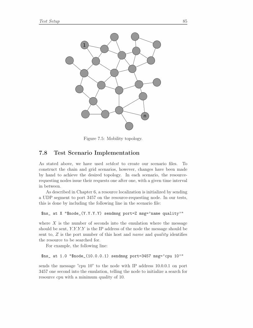
Test Setup 85
1
n
Figure 7.5: Mobility topology.
7.8 Test Scenario Implementation
As stated above, we have used setdest to create our scenario files. Toconstruct the chain and grid scenarios, however, changes have been madeby hand to achieve the desired topology. In each scenario, the resource-requesting nodes issue their requests one after one, with a given time intervalin between.
As described in Chapter 6, a resource localization is initialized by sendinga UDP segment to port 3457 on the resource-requesting node. In our tests,this is done by including the following line in the scenario file:
$ns_ at X "$node_(Y.Y.Y.Y) sendmsg port=Z msg=’name quality’"
where X is the number of seconds into the emulation where the messageshould be sent, Y.Y.Y.Y is the IP address of the node the message should besent to, Z is the port number of this host and name and quality identifiesthe resource to be searched for.
For example, the following line:
$ns_ at 1.0 "$node_(10.0.0.1) sendmsg port=3457 msg=’cpu 10’"
sends the message ”cpu 10” to the node with IP address 10.0.0.1 on port3457 one second into the emulation, telling the node to initialize a search forresource cpu with a minimum quality of 10.
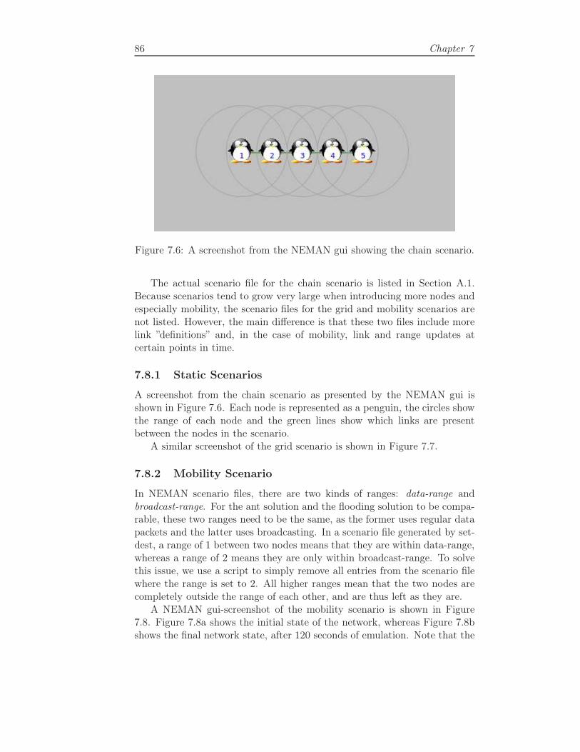
86 Chapter 7
Figure 7.6: A screenshot from the NEMAN gui showing the chain scenario.
The actual scenario file for the chain scenario is listed in Section A.1.Because scenarios tend to grow very large when introducing more nodes andespecially mobility, the scenario files for the grid and mobility scenarios arenot listed. However, the main difference is that these two files include morelink ”definitions” and, in the case of mobility, link and range updates atcertain points in time.
7.8.1 Static Scenarios
A screenshot from the chain scenario as presented by the NEMAN gui isshown in Figure 7.6. Each node is represented as a penguin, the circles showthe range of each node and the green lines show which links are presentbetween the nodes in the scenario.
A similar screenshot of the grid scenario is shown in Figure 7.7.
7.8.2 Mobility Scenario
In NEMAN scenario files, there are two kinds of ranges: data-range andbroadcast-range. For the ant solution and the flooding solution to be compa-rable, these two ranges need to be the same, as the former uses regular datapackets and the latter uses broadcasting. In a scenario file generated by set-dest, a range of 1 between two nodes means that they are within data-range,whereas a range of 2 means they are only within broadcast-range. To solvethis issue, we use a script to simply remove all entries from the scenario filewhere the range is set to 2. All higher ranges mean that the two nodes arecompletely outside the range of each other, and are thus left as they are.
A NEMAN gui-screenshot of the mobility scenario is shown in Figure7.8. Figure 7.8a shows the initial state of the network, whereas Figure 7.8bshows the final network state, after 120 seconds of emulation. Note that the

Test Setup 87
Figure 7.7: A screenshot from the NEMAN gui showing the grid scenario.
ranges of the nodes are left out, as for some reason, the ranges generatedby setdest do not always correspond with the physical node locations, alsoprovided by setdest — sometimes we get a link between nodes that shouldhave been outside the range of each other.
7.9 Workload
The workload is the load that is put on the system during usage. We maydiffer between two kinds of workload: test workload and real workload [17].The real workload is the workload that the system will be exposed to duringnormal operation, whereas the test workload is the workload under whichthe system is tested, and which is used to compare different systems. Forthe tests to give as realistic results as possible, the test workload should besimilar to the real workload. The test workload may, however, just like testscenarios, be simplified to ease the configuration of the workload.
In our experiments, the workload is made up by the number of resource-holding nodes, resource-requesting nodes, number of requests and node lo-cation and mobility. As stated in the design assumptions in Section 5.2, weassume that both resource-requesting and resource-holding nodes are ran-domly placed within the MANET. To reflect this, we should place these atrandom positions in our scenarios. However, because we need our tests to

88 Chapter 7
(a) Initial state.
(b) Final state.
Figure 7.8: Screenshots from the NEMAN gui showing the mobility scenario.

Test Setup 89
be repeatable, random placement is not desireable. Instead, we have triedto place them as ”randomly” as possible. This will be further explained foreach scenario below.
In all scenarios, we have, for simplicity, restricted ourselves to onlyone resource-holding node per MANET. The number of resource-requestingnodes varies, as explained below. Tests are divided between single location,with only one resource-requesting node, and location learning, where thereare several resource-requesting nodes. In all experiments, the requestingnode is looking for a resource named ”memory” with a quality of at least90. The resource-holding node holds a resource with name ”memory” and aquality 100 + its tap number, thus, resource memory at tap number 4 hasa quality of 104. The only reason for this is to make it easier to verify whenreading output files that the resource was located at the correct node — theonly actual requirement is that the quality is ≥ 90.
7.9.1 Parameters
For all tests, we have set the time to live value for all ants and floodedmessages equal to the number of nodes in the network minus one. If thisvalue is too small, the possibility that an ant actually finds a resource issmall, as it might never get to walk far enough. If the value is too large,we risk that ants ”get lost” in parts of the network where the resource is notpresent. We have chosen to set this value equal to the number of nodes inthe MANET. The ant should then have the possibility to walk the entirediameter of the network, but still not walk ”forever”.
The expiry time of learned resource location information is set to infinity.This is a rather unrealistic value, but makes our test cases simpler.
The max_sleep_time for the ant solution is set to 2 seconds.
7.9.2 Scenario Properties
Chain Scenario
As this is a static scenario, the size of the area in which the network islocated is unimportant. The scenario consists of five nodes linked togetherin a chain. The purpose of this setup is mainly to show that the algorithm issound and the functionality works as expected. Because of the characteristicsof the chain topology, we do not conduct any experiments with more thanone requesting node.
Grid Scenario
Our grid scenario consists of 25 nodes, in a 5 x 5 grid.

90 Chapter 7
1 2 3 4 5
Figure 7.9: A chain topology with requesting and resource-holding nodes atthe ends. A dashed line represents a requester, and a dotted line representsa resource holder.
Mobility Scenario
This scenario consists of 25 mobile nodes. These move within an area ofsize 700m x 700m, with a maximum speed of 15 metres per second and amaximum pause time of 8 seconds for a duration of 120 seconds.
7.9.3 Single Localization
In these experiments, we use one resource-requesting and one resource-holdingnode for all three scenarios.
Chain Scenario
In our simplest experiments, we use a chain with five nodes, where we placethe requesting node at one end of the chain and the requested node in theother end, as shown in Figure 7.9.
Grid Scenario
There are several possibilities when it comes to placing the requesting node aswell as the resources requested in the grid. With only one available resource,one possibility is to place the requesting node and the requested resource indiagonally opposite corners. To obtain a more ”random” placement of thesetwo nodes, we have placed them one hop into the network, giving them fourinstead of two neighbors, as shown in Figure 7.10, which is more likely thana real corner placement with only two neighbors. Thus, in the figure, node7 is the requesting node and node 19 is the resource-holding node.
Mobility Scenario
In an experiment with one single localization, we do not really experienceany effects of the mobility. We have still included this experiment for com-pleteness’ sake. The scenario also provides a picture of how the ant solutionbehaves in a network with a more irregular topology, where some nodes havefew neighbors and others may have more neighbors.
Resource-requesting and resource-holding nodes have been chosen suchthat intially the shortest path between them is 4 hops, as this gives a largenumber of possible paths for the forward ant. Thus, this case is quite similarto the grid scenario when performing only one localization. The position of

Test Setup 91
1 2 3 4 5
11 12 13 14 15
21 22 23 24 25
Figure 7.10: A grid topology with 25 nodes: One requesting node (node 7)and one resource-holding node at diagonally opposite ”corners”. A dashedline represents a requester, and a dotted line represents a resource holder.
these nodes are shown in Figure 7.11, where node 12 is the requesting nodeand node 4 is the resource-holding node.
7.9.4 Location Learning
In this range of test scenarios, we introduce several resource-requesting nodes.These all request exactly the same resource. Thus, in the ant solution, assoon as the first forward ant has located the resource, the location informa-tion starts spreading throughout the network.
Grid Scenario
To show the real effect of the ant approach and resource location learning,we use a grid with three different requesting nodes. These are placed in near-”corners” (nodes 7, 9, and 17) except for the one holding the resource-holdingnode (node 19), as shown in figure 7.12. The shortest path from these nodesto the resource-holding node is thus 4, 2 and 2 hops, respectively.
The requesting nodes issue their requests in numerical order, startingwith the lowest numbered node. Requests are issued every 15 seconds, givingeach node up to 8 tries to locate the given resource before the next nodestarts. If the first node does not locate the resource in 8 tries, the requestingnodes will continue resource localization simultaneously.

92 Chapter 7
Figure 7.11: A mobility topology with 25 nodes; One resource-requestingnode (node 12) and one resource-holding node (node 4). A dashed circlerepresents a requester, and a dotted circle represents a resource holder.

Test Setup 93
1 2 3 4 5
11 12 13 14 15
21 22 23 24 25
Figure 7.12: A grid topology with 25 nodes; Three resource-requesting nodes(nodes 7, 9 and 17). one resource-holding node (node 19). A dashed linerepresents a requester, and a dotted line represents a resource holder.
Mobility Scenario
Initially, the resource-requesting nodes are placed around the edge, andthe resource-holding node in the ”middle”. We use five different resource-requesting nodes, each requesting a resource with 25 seconds in between.This gives nodes time to move a bit around between each search, and thusspreading any learned location information. However, even if requestingnodes were initially placed around the edge, this may have changed be-fore they actually get to issue a request. The scenario with requesting andresource-holding nodes in their initial positions is shown in Figure 7.13.
Like in the grid scenario, nodes receive the initial resource requests innumerical order, starting with the lowest numbered node. To give nodes timeto move around a bit between each initiated resource localization, requestsare issued by different requesting nodes every 25 seconds.

94 Chapter 7
Figure 7.13: A mobility topology with 25 nodes; One resource-holding node(node 22) and five resource-requesting nodes (nodes 4, 5, 6, 10 and 25). Adashed circle represents a requester, and a dotted circle represents a resourceholder.

Chapter 8
Performance Evaluation
”Software and cathedrals are much the same — first we build
them, then we pray.”
— Sam Redwine
In this chapter we present the results from our performance tests. Westart by explaining some factors that may have an impact on the tests results.Then we compare the results from the ant and flooding solutions, and lookat which solution performs best in each test scenario and analyze why thesolutions perform as they do. We also give a few suggestions to what may bedone differently to address some of the problems observed when analyzingthe test results.
8.1 Influencing Factors
8.1.1 Topology Initialization and Updates
During our testing, we have experienced some problems with OLSR usinga very long time to get all topology information and set up routes. In thevery simple chain scenario with only five nodes, it took up to 15 secondsto establish a route between nodes 1 and 5. For the ant solution, this isnot a problem, as ants move between neighbors, and neighbor informationappears much faster than longer distance routes. However, for the floodingsolution’s resource replies to get delivered from the resource-holding to theresource-requesting nodes, we need several hops-routes to be established.
To solve this, we have introduced a delay between the time a scenariois started and the first resource request is sent from the scenario file to aresource-requesting node. In the stationary scenarios this is trivial, as thenetwork looks the same after 30 seconds as it did when the scenario wasstarted. In the mobility scenario, however, the node positions may be very

96 Chapter 8
different after 30 seconds. In the single localization mobility scenario, this isnot a problem, as we still do not exploit the mobility. Note, however, thatthe topology when the resource request is sent is not the same as the initialtopology shown in Figure 7.11.
In the location learning mobility scenario, however, we ”loose” 30 secondsof mobility, leaving less time to allow nodes to move in between resourcelocalizations. To avoid this, we have added 30 seconds of non-mobility tothis scenario file between the node range initialization and the first rangeupdates. Thus, this scenario actually lasts for 150 seconds instead of 120,but only the last 120 seconds are exploited by the ant and flooding solutions.
In Section 7.6.1, we stated that during performance testing, we will onlybe concerned with successful tests. In Section 6.6.3, we stated that nodemobility should not be a problem for the ant solution, as any lost neighborswould be handled by the routing protocol. It turns out, however, that atsome occasions, topology updates are too slow, and some ants are thus lostwhen a node tries to forward it to a newly lost neighbor. Unfortunately,time issues inhibited us in adjusting the code to this. During our testing,this happened in around 2 out of 10 single test runs. The experiments wherethis occurred do not count as ”successful”: If an ant is lost, a new forwardant will be sent by the requesting node, so a resource will still eventuallybe found if present. However, the system will count the lost ant as an antreaching time to live = 0 and assume it has traveled its maximum numberof hops, which may not be correct. To get as correct performance results aspossible, we have thus left out those experiments where an ant is lost. Wehave thus run more than 10 experiments in these cases, and left out thosewhere an ant was lost due to transmission errors. Making the ant solutionmore robust to such transmission errors is thus left as further work.
8.1.2 Time Inaccuracy
The timing of one resource localization has been performed by using thegettimeofday() function. This is possible without any clock synchroniza-tion as the whole system is running on the same machine. However, due todifferences in the ant and flooding solution source code, it is not possibleto start and stop these measurements at the exact same position in bothsystems. Thus, these are approximate times.
8.1.3 Average Neighborhood Size
For the chain and grid scenarios, the number of neighbors per node is con-stant, as there is no mobility or link changes. In the chain scenario, theaverage number of neighbors per node is 1.6, and in the grid scenario theaverage number of neighbors per node is the double, namely 3.2. In themobility scenarios, however, the number of neighbors per node varies over
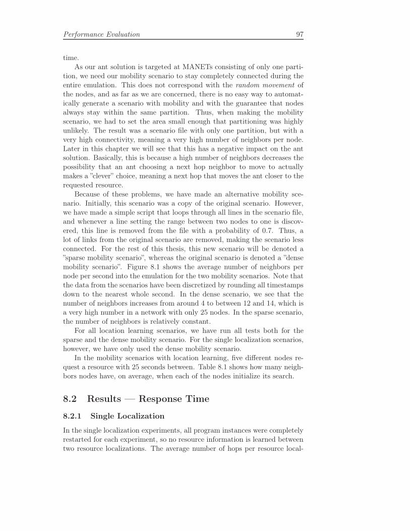
Performance Evaluation 97
time.As our ant solution is targeted at MANETs consisting of only one parti-
tion, we need our mobility scenario to stay completely connected during theentire emulation. This does not correspond with the random movement ofthe nodes, and as far as we are concerned, there is no easy way to automat-ically generate a scenario with mobility and with the guarantee that nodesalways stay within the same partition. Thus, when making the mobilityscenario, we had to set the area small enough that partitioning was highlyunlikely. The result was a scenario file with only one partition, but with avery high connectivity, meaning a very high number of neighbors per node.Later in this chapter we will see that this has a negative impact on the antsolution. Basically, this is because a high number of neighbors decreases thepossibility that an ant choosing a next hop neighbor to move to actuallymakes a ”clever” choice, meaning a next hop that moves the ant closer to therequested resource.
Because of these problems, we have made an alternative mobility sce-nario. Initially, this scenario was a copy of the original scenario. However,we have made a simple script that loops through all lines in the scenario file,and whenever a line setting the range between two nodes to one is discov-ered, this line is removed from the file with a probability of 0.7. Thus, alot of links from the original scenario are removed, making the scenario lessconnected. For the rest of this thesis, this new scenario will be denoted a”sparse mobility scenario”, whereas the original scenario is denoted a ”densemobility scenario”. Figure 8.1 shows the average number of neighbors pernode per second into the emulation for the two mobility scenarios. Note thatthe data from the scenarios have been discretized by rounding all timestampsdown to the nearest whole second. In the dense scenario, we see that thenumber of neighbors increases from around 4 to between 12 and 14, which isa very high number in a network with only 25 nodes. In the sparse scenario,the number of neighbors is relatively constant.
For all location learning scenarios, we have run all tests both for thesparse and the dense mobility scenario. For the single localization scenarios,however, we have only used the dense mobility scenario.
In the mobility scenarios with location learning, five different nodes re-quest a resource with 25 seconds between. Table 8.1 shows how many neigh-bors nodes have, on average, when each of the nodes initialize its search.
8.2 Results — Response Time
8.2.1 Single Localization
In the single localization experiments, all program instances were completelyrestarted for each experiment, so no resource information is learned betweentwo resource localizations. The average number of hops per resource local-

98 Chapter 8
5
6
7
8
9
10
11
12
13
14
0 20 40 60 80 100 120
Num
ber
of n
eigh
bors
Seconds into emulation
Dense scenario Sparse scenario
Figure 8.1: Average number of neighbors per second into the simulation inthe mobility scenarios.
Request number 1 2 3 4 5
Dense scenario 5.52 9.36 12.0 12.4 12.48Sparse scenario 5.52 6.32 6.4 6.4 6.4
Table 8.1: Average number of neighbors per node in the dense and sparsemobility scenarios when requests are issued.

Performance Evaluation 99
Solution Chain Scenario Grid Scenario Mobility
ant 4.0 21.0 51.8flood 4.0 4.0 2.0
Table 8.2: Average number of hops used in one resource localization in eachscenario.
Solution Chain Scenario Grid Scenario Mobility
ant 13.02 848.8 3130.0flood 1.5 14.3 13.2
Table 8.3: Average time in milliseconds spent on one resource localization ineach scenario.
ization for each scenario is shown in Table 8.2, and the average time spentper resource localization for each scenario is shown in Table 8.3.
Chain Scenario
As we expected, the two solutions use the same number of hops in the verysimple chain scenario. This scenario consists of five nodes that all need tobe visited to find the resource in the other end, giving four hops. This fitsperfectly with the observed results.
For the time spent, however, we see that the flooding solution uses lesstime than the ant solution: The ant solution uses almost nine times moretime than the flooding solution. This is probably due to the fact that theant solution requires quite a lot more processing in each intermediate nodethan the flooding solution, which only re-broadcasts received messages. Theant solution also handles incoming topology updates, and thus simply hasmore to do than the flooding solution.
Grid Scenario
For the grid scenario, the difference in the response time for the two solutionsreally starts to show. The response time in number of hops is 7.7 times aslarge in the ant solution as in the flooding solution. As expected, the floodingsolution still uses 4.0 hops, which is the length of the shortest path fromthe resource-requesting to the resource-holding node, in average to localizea resource. The ant solution uses almost 60 times as much clock time tolocalize a resource as the flooding solution.

100 Chapter 8
Mobility Scenario
In these scenarios, the difference between the response time in the ant so-lution and the flooding solution gets even more significant. The floodingsolution, which always reaches the resource-holding node in the shortestpossible number of hops, has a response time of 2 hops in the dense scenario,whereas the ant solution uses on average 51.8 hops, or almost 26 times morehops than the flooding solution. In the sparse scenario, the flooding solutionuses 3.2 hops, whereas the ant solution uses 105.67 hops, approximately 33times as many as the flooding solution. The same is shown by the measuredtimes: In the sparse scenario, the ant solution uses a whooping 381.69 timeslonger to locate the given resource.
This is a scenario with mobility. However, as we are only performingone resource localization, the duration of an experiment is too short for themobility to make a difference on the results. However, there is a possibilitythat the topology changes between two subsequent forward ants if more thanone is needed. The network topology might thus be different when the lastforward ant is sent than it was during the resource localization in the floodingsolution, making the minimum number of hops smaller or larger.
8.2.2 Location Learning
Grid Scenario
Figure 8.2 shows the average response time against the number of requestingnodes in the grid scenario with location learning. The response time asnumber of hops is shown in Figure 8.2a, and the response time in millisecondsis shown in Figure 8.2b. Response times are plotted per resource-requestingnode, thus the first pair of columns shows average response time for thefirst requesting node, the second pair of columns shows the average responsetime for the second requesting node and so on. Note also that the responsetimes in both figures are plotted with base 2 logarithmic scale. This is donebecause of the large span in response time results: When using a linearscale, most results do not show on the plot because of the large difference inresponse time from the first resource-requesting node in the ant solution toall subsequent resource-requesting nodes in the ant solution and all floodingsolution results.
From the plot, we see that for the ant solution, the tendency in thisscenario is quite clear: The response time, both in number of hops as wellas in milliseconds, decreases drastically from the first, with 40.2 hops, tothe second requesting node, with 3.5 hops. From the second to the thirdrequesting node, there is little difference, and we actually see a small increasein number of hops, but a small decrease in number of seconds.
For the flooding solution, however, we get the expected results: Thefirst requesting node uses more hops, but this is due to the fact that the

Performance Evaluation 101
1
2
4
8
16
32
64
1 2 3
Num
ber
of h
ops
used
Requesting node number
Ant solutionFlood solution
(a) Number of hops.
0.25 1 4
16 64
256 1024 4096
1 2 3
Tim
e us
ed (
seco
nds)
Requesting node number
Ant solutionFlood solution
(b) Number of milliseconds.
Figure 8.2: Average response time per resource-requesting node in grid sce-nario with location learning. Note: y-axis plotted with base 2 logarithmicscale.
0.25
1
4
16
64
1 2 3 4 5
Num
ber
of h
ops
used
Requesting node number
Ant solutionFlood solution
(a) Number of hops.
4 8
16 32 64
128 256 512
1024 2048 4096 8192
1 2 3 4 5
Tim
e us
ed (
seco
nds)
Requesting node number
Ant solutionFlood solution
(b) Number of milliseconds.
Figure 8.3: Average response time per resource-requesting node in densemobility scenario with location learning. Note: y-axis plotted with base 2logarithmic scale.
first requesting node is located 4 hops away from the resource-holding node,whereas the second and third are only two hops away. In one of the floodexperiments, one flooded package from the second requesting node reachedthe resource-holding node via a longer path before the one traveling theshortest path. The flooding solution only handles the first incoming copyof the same message, thus, there is a slight difference between the averagenumber of hops for the second (2.2 hops) and the third (2 hops) requestingnode.
Mobility Scenario — Dense
In Figure 8.3, we see how the average response time per resource localizationchanges with the number of nodes requesting the same resource. Figure 8.3ashows the response time in number of hops, whereas Figure 8.3b shows thenumber of milliseconds spent.
We see here the same tendency as we saw in the grid scenario: Thereis a dramatic decrease in the response time from the first to the second
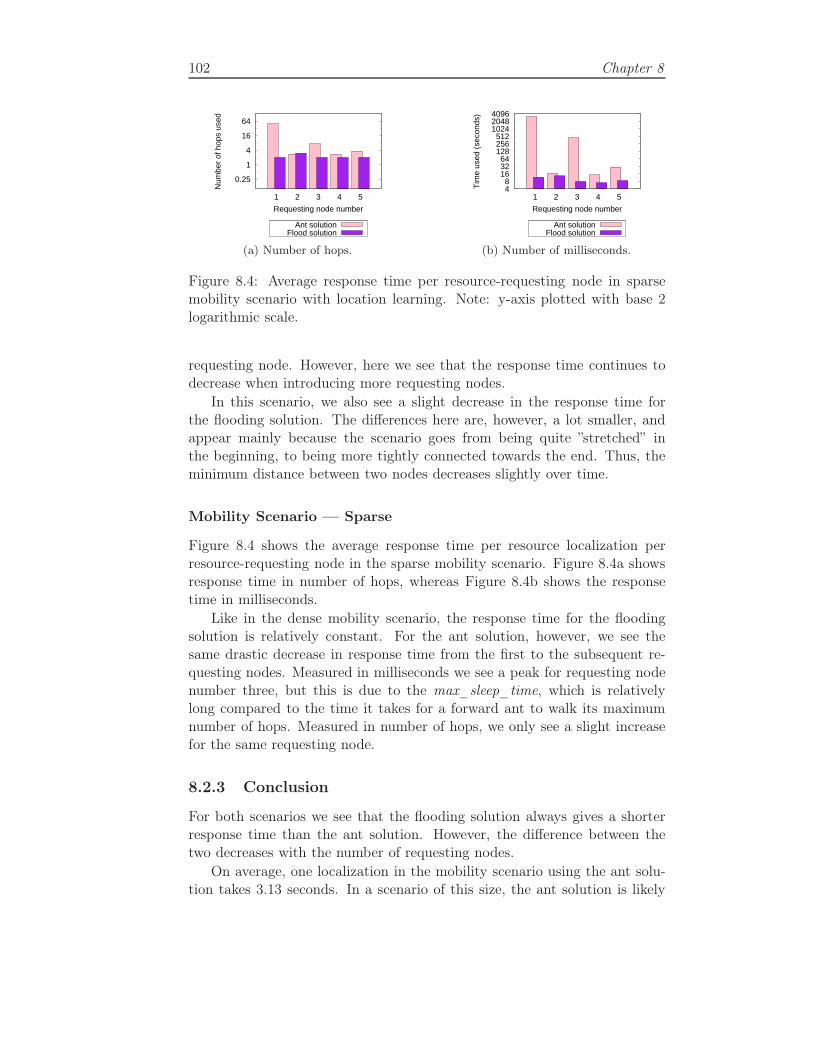
102 Chapter 8
0.25
1
4
16
64
1 2 3 4 5
Num
ber
of h
ops
used
Requesting node number
Ant solutionFlood solution
(a) Number of hops.
4 8
16 32 64
128 256 512
1024 2048 4096
1 2 3 4 5
Tim
e us
ed (
seco
nds)
Requesting node number
Ant solutionFlood solution
(b) Number of milliseconds.
Figure 8.4: Average response time per resource-requesting node in sparsemobility scenario with location learning. Note: y-axis plotted with base 2logarithmic scale.
requesting node. However, here we see that the response time continues todecrease when introducing more requesting nodes.
In this scenario, we also see a slight decrease in the response time forthe flooding solution. The differences here are, however, a lot smaller, andappear mainly because the scenario goes from being quite ”stretched” inthe beginning, to being more tightly connected towards the end. Thus, theminimum distance between two nodes decreases slightly over time.
Mobility Scenario — Sparse
Figure 8.4 shows the average response time per resource localization perresource-requesting node in the sparse mobility scenario. Figure 8.4a showsresponse time in number of hops, whereas Figure 8.4b shows the responsetime in milliseconds.
Like in the dense mobility scenario, the response time for the floodingsolution is relatively constant. For the ant solution, however, we see thesame drastic decrease in response time from the first to the subsequent re-questing nodes. Measured in milliseconds we see a peak for requesting nodenumber three, but this is due to the max_sleep_time, which is relativelylong compared to the time it takes for a forward ant to walk its maximumnumber of hops. Measured in number of hops, we only see a slight increasefor the same requesting node.
8.2.3 Conclusion
For both scenarios we see that the flooding solution always gives a shorterresponse time than the ant solution. However, the difference between thetwo decreases with the number of requesting nodes.
On average, one localization in the mobility scenario using the ant solu-tion takes 3.13 seconds. In a scenario of this size, the ant solution is likely

Performance Evaluation 103
to need more than one forward ant to locate a resource because an ant’stime to live-value reaches 0. The response time in milliseconds is thus highlydependent on the size of max_sleep_time, the time before a forward antis considered unsuccessful by the requesting node and a new forward antis sent. As the max_sleep_time between two forward ants in our tests is 2seconds, this tells us that in this scenario, the ant solution on average neededmore than one forward ant to locate the resource (it is highly unlikely thatthe first ant used such a large amount of time to move the maximum of25 hops). Thus, had the max_sleep_time been different, then the responsetime would be equally different.
Another observation is that the ant solution performs particularly badin the mobility scenarios, especially in the single location case but also inthe location learning case, there especially for the first requesting node. InSection 8.1.3, we saw that the number of neighbors per node is a lot higherin the dense mobility scenario than in the other two scenarios, and also abit higher in the sparse mobility scenario. For a forward ant, this meansthat when standing in a node selecting which neighbor to use as next hop,it has a high number of neighbors to choose from. With only one resource-holding node present in the entire network, the chance of making a cleverchoice in this situation decreases with the number of neighbors. From thetcpdump files from the mobility scenario, we see that in many cases, thefirst requesting node may have to send up to six forward ants to look for thesame resource before it is actually located. The reason for this is that thereare too many available neighbors and thus too little chance of making the”right” choice — the forward ant needs a bit of luck to be able to locate theresource fast. The node needs more tries to find out which paths lead to theresource and which paths do not.
This is also reflected by the difference between the two mobility scenarios:For the first requesting node, the number of hops is 69.7 and 50.1 for thedense and sparse scenarios respectively. There is thus a decrease in thenumber of hops needed in the sparse scenario. The much smaller number ofneighbors in the sparse scenario increases the possibility that a forward antmakes a ”smart” choice when choosing a next hop. As soon as the locationlearning kicks in, there is little difference between the sparse and the densescenario.
8.3 Results — Bandwidth Usage
8.3.1 Single Localization
The results from our bandwidth experiments are shown in Tables 8.4 and8.5, under ”Messages Sent” and ”Bytes Sent”. These show the total numberof messages and bytes that were, in some way, sent from all nodes in thescenario during the different scenarios. By ”sent”, we mean both from our

104 Chapter 8
Scenario Solution Messages Sent Messages Received Utilization
ChainAnt 8.0 14.0 57.14
Flood 8.0 14.0 57.14
GridAnt 26.7 91.7 29.12
Flood 35.0 92.0 38.04
MobilityAnt 56.6 660.1 8.57
Flood 40.0 271.0 14.76
Table 8.4: Messages sent and received and message utilization for both so-lutions in each single localization scenario.
Scenario Solution Bytes Sent Bytes Received Utilization
ChainAnt 1216.0 2128.0 57.14
Flood 524.0 1400.0 57.14
GridAnt 6584.0 22440.0 29.34
Flood 3604.0 9680.0 37.23
MobilityAnt 15940.8 186308.8 8.56
Flood 4064.0 28852.0 14.09
Table 8.5: Bytes sent and received and message utilization for both solutionsin each single localization scenario.
application as well as those messages that were only forwarded to other nodeson the transport layer.
Note that as a neighbor may be lost between the forwarding of a forwardant and the reception of the corresponding ant, as explained in Section 6.6.3,the number of sent messages may be slightly larger than the actual numberof nodes visited by the forward ant, as the backward ant may need to beforwarded via other nodes to reach the lost neighbor.
If we look at the number of bytes sent, we see that in each scenario, theflooding solution performs significantly better than the ant solution, eventhough the ant solution nodes sent less messages in the grid scenario. Thisis due to the large message size in the ant solution: A forward ant is initially128 bytes large, whereas a flood solution resource request is only 108 bytes.In addition to this, the size of a forward ant increases for every hop as addressinformation for the last hop is appended. The size of one unit of addressinformation is 16 bytes. Thus, the size of a forward ant increases linearlywith 16 bytes per hop, whereas the size of a flood request is constant. Figure8.5 shows the relationship between ant and flooding solution message sizesduring resource search (backward ant/resource reply not included). The size

Performance Evaluation 105
0
100
200
300
400
500
5 10 15 20
Mes
sage
siz
e
Number of hops
Ant solutionFlooding solution
Figure 8.5: Message size during resource search in both solutions plottedagainst the number of hops traveled.
of a backward ant is the same as a forward ant, as these use the same datastructure. The only difference is that the size of the backward ant decreaseswith the number of hops. A flood resource reply, on the other hand, is only92 bytes.
Note also that these sizes are including some information needed fortesting purposes, and may be removed during normal system use.
8.3.2 Location Learning
Tables 8.6 and 8.7, columns ”Messages Sent” and ”Bytes Sent” respectively,show the number of messages and bytes sent in each of the location learningscenarios. Again, we see that the ant solution benefits from the introduc-tion of location learning, as in all three scenarios, the ant solution performssignificantly better than the flooding solution with respect to the number ofmessages sent: The flooding solution nodes send approximately 61% moremessages than the ant solution nodes in the dense scenario and 88% moremessages in the sparse scenario. However, like in the single localization sce-narios we see that the large size of the ant still makes the ant solution senda significantly higher number of bytes than the flooding solution.
When comparing the results from the two mobility scenarios, we see thatthe sparse scenario gives better performance than the dense scenario: Nodesin the ant solution send approximately 18% more messages in the dense thanin the sparse scenario. This is probably due to the difference in number ofneighbors: Fewer neighbors increases the possibility of choosing the ”correct”neighbor as next hop. For the flooding solution, the numbers are more orless equal.

106 Chapter 8
Scenario Solution Messages Sent Messages Received Utilization
GridAnt 57.0 195.2 29.2
Flood 88.1 258.8 34.04
M-DenseAnt 91.9 763.1 12.04
Flood 148.4 1316.0 11.28
M-SparseAnt 77.7 553.0 14.05
Flood 146.0 813.6 17.94
Table 8.6: Messages sent and received and message utilization for both so-lutions in each location learning scenario. M-dense and M-sparse are denseand sparse mobility scenarios, respectively.
Scenario Solution Bytes Sent Bytes Received Utilization
GridAnt 14291.2 48908.8 29.22
Flood 9257.2 27457.6 33.71
M-DenseAnt 24612.8 193644.8 12.71
Flood 15572.4 140800.0 11.06
M-SparseAnt 19454.4 137593.6 14.14
Flood 15352.0 86867.2 17.67
Table 8.7: Bytes sent and received and message utilization for both solutionsin each location learning scenario. M-dense and M-sparse are dense andsparse mobility scenarios, respectively.
Performance Evaluation 107
8.3.3 Conclusion
What the bandwidth tests show us is that the ant solution has the potentialto outperform the flooding solution when the network size and/or the numberof requesting nodes increase. Increasing network size causes a higher degreeof flooding, whereas the number of nodes requesting nodes has an impacton how much we get out of the resource location learning. However, in alltest scenarios, the large ant size causes the ant solution to behave poorlywith respect to the number of bytes sent. As stated in Chapter 6, the antdata structure is not optimized with respect to size, and it should thus bepossible to decrease the size of the ants. However, there will always be aneed of appending address information to forward ants for the correspondingbackward ant to be able to retrace its path. Thus, the size of a forward antwill always have to increase with the number of hops traveled. However, onemight consider other, better scalable ways to store this information than the16 bytes large sockaddr_in structure that is currently used.
Also, in our experiments, the ant time to live was equal to the numberof nodes in the network minus one. This means that our ants are allowed togrow from 128 bytes to 496 bytes, or almost four times its own size, in thegrid and mobility scenarios consisting of 25 nodes. From our results, we seethat the time to live-value should probably be set to a smaller number. Bydoing this, we limit the maximum size of a forward ant. However, we alsomake it harder for a forward ant to find the resource during its search, as itis allowed to visit a smaller number of nodes.
Another interesting observation is that if we compare the results fromthe ant solution response time measurements in number of hops with thecorresponding number of sent messages, we see that the latter numbers areonly slightly smaller than the former. Remember that the response time ismeasured from a forward ant is sent from the resource-requesting node tothe resource-holding node is reached, whereas the number of sent messagesalso includes the backward ant. If we did not eliminate loops traveled bythe forward ant before sending the corresponding backward ant, we wouldexpect the number of sent messages to be approximately twice as large asthe number of hops traveled by the forward ant. However, as any loopsare eliminated, the number of hops traveled by the backward ant, and thusthe number of sent messages, may be lower than that of the correspondingforward ant.
If we look at the chain scenario with a single requesting node, we see thatthe number of hops is 4.0 and the number of sent messages is 8.0, exactlytwice as much. This fits well with what we expect for this scenario, as thecharacteristics of the chain scenario makes it impossible for the forward antto travel in loops. For the grid scenario, however, the number of hops is21.0, whereas the number of sent messages is 26.7, only approximately 21%larger. Thus, the length of the path traveled by the backward ant back to

108 Chapter 8
the requesting node is drastically reduced. The reason for this is that theforward ant traveled in a long loop, which was later eliminated. The sameholds for the mobility scenario, where the number of sent messages is onlyapproximately 9% larger than the number of hops.
This will have an impact on the results we get from location learning. Thegain from this concept is highly dependent of the learned location informationspreading to as many nodes as possible, rising the possibility for subsequentants searching for similar resources reaching nodes with resource locationinformation. However, by decreasing the length of the path traveled bythe backward ant, we limit the number of nodes picking up the new locationinformation. Thus, from these results, we see that one might want to considerallowing also backward ants to travel in loops.
Loops were eliminated because we wanted to use as little bandwidth andprocessing power as possible to get the backward ant to the requesting node.Thus, we are dealing with a tradeoff: We can either spend less resources, orwe can get a good location information spreading. Which approach to usedepends on the application: If it is likely that several subsequent ants lookfor similar resources, a good location information dissemination could weighup for the expensive first localization. If, in most cases, only one node will berequesting a certain resource, however, most requests will be expensive first-time requests, and we do not get to utilize the well-disseminated locationinformation.
8.4 Results — Processing Power Usage
Processing power usage is measured in the number of received messages,thus the number of messages that, in some way, need to be handled by thereceiving node. This includes both messages that are delivered all the way upto the application layer as well as those that are received but only forwardedor discarded at the transport layer.
In the ant solution, we expect the number of sent messages from theapplication level to be equal to the number of received messages, as all nodesreceiving an ant should either re-forward it or, if the ant is a forward ant andthe resource is present: Reply with a backward ant. An intuitive thought isthat if a forward ant ”dies” because of a too low time to live-value, there willonly be a received message, not a sent message. However, this will lead tothe requesting node sending a new forward ant. This node will only get onereply back, though, thus the extra sent message from the requesting node”eliminates” the extra received message at the node receiving the forwardant with time to live = 0.
However, as mentioned above, these results contain both application layerand network layer messages. As stated earlier, the ant solution does not ex-ploit the fact that all nodes within range of a transmitting node will overhear

Performance Evaluation 109
the transmitted package and have to check if it is destined for itself or someother node. In the flooding solution, however, all nodes hearing a messagepick it up, but only retransmit if an equal message has not already beenreceived and retransmitted.
8.4.1 Single Localization
The results from our single localization experiments are shown in Table 8.4,column ”Messages Received” and 8.5, column ”Bytes Received”.
Chain Scenario
As expected, the number of received messages is equal for both solutions inthe chain scenario, as all messages follow the exact same path. As observedin the above bandwidth experiments, the number of bytes is quite a bit largerfor the ant solution than for the flooding solution, again because of the muchlarger ant solution message size.
Grid Scenario
In the grid scenario, the two solutions perform approximately equally; theant solution receives on average 0.3 messages less than the flooding solution.As the network size and number of hops needed increases, the number ofbytes also increases, and the difference between the ant solution and theflooding solution is even larger than in the chain scenario.
Mobility Scenario
In the mobility scenario, however, the number of received messages in theant solution increases dramatically, and is approximately 2.4 times higherthan that of the flooding solution. This is also shown in the number of bytesreceived, and in this scenario, the nodes in the ant solution receives approx-imately 6.5 times as many bytes as the nodes in the flooding solution. Thelarge increase is due to the large number of neighbors receiving everythingtransmitted from their neighbors.
8.4.2 Location Learning
The results from the location learning experiments are listed in Table 8.6and 8.7 under the columns ”Messages Received” and ”Bytes Received” re-spectively.
Grid Scenario
The flooding solution here uses approximately 32.6% more messages to lo-calize the requested resources. When measuring in number of bytes, the

110 Chapter 8
0 20 40 60 80
100
Chain
GridM
obility
Per
cent
age
Scenario
Ant solutionFlood solution
(a) Message utilization
0 20 40 60 80
100
Chain
GridM
obility
Per
cent
age
Scenario
Ant solutionFlood solution
(b) Byte utilization
Figure 8.6: Total utilization percentage in each scenario.
ant solution is still outperformed by the flooding solution, as the ant solu-tion nodes receive approximately 78% more bytes than the flooding solutionnodes.
Mobility Scenario
In the dense scenario, the flooding solution nodes receive 72.5% more mes-sages than the ant solution, but still the ant solution nodes receive 37.5%more bytes. In the sparse scenario, the difference is smaller, but the floodingsolution still receives approximately 47% more messages. We also see thesame as in the bandwidth usage experiments: The ant solution performsbetter in the sparse scenario than in the dense: Nodes in the dense scenarioreceive approximately 38% more messages than nodes in the sparse scenario.
8.4.3 Conclusion
In these experiments, we see the same tendency as in the bandwidth exper-iments: When introducing more requesting nodes, the ant solution localizesthe requested resource using less resources than the flooding solution, giventhat we measure in number of messages. Still, the ant size makes the antsolution perform quite a bit worse than the flooding solution with respect tothe number of bytes received. We also see that the ant solution benefits fromhaving a low number of neighbors, as for local processing powers, a lowernumber of neighbors means a lower number of overheard messages.
8.5 Results — Processing Power Utilization
The local processing power utilization is the ratio of sent messages to receivedmessages, and expresses the percentage of received messages that a nodefound worth either forwarding or replying to, meaning the messages that thenode received and actually used to contribute to the resource localization.
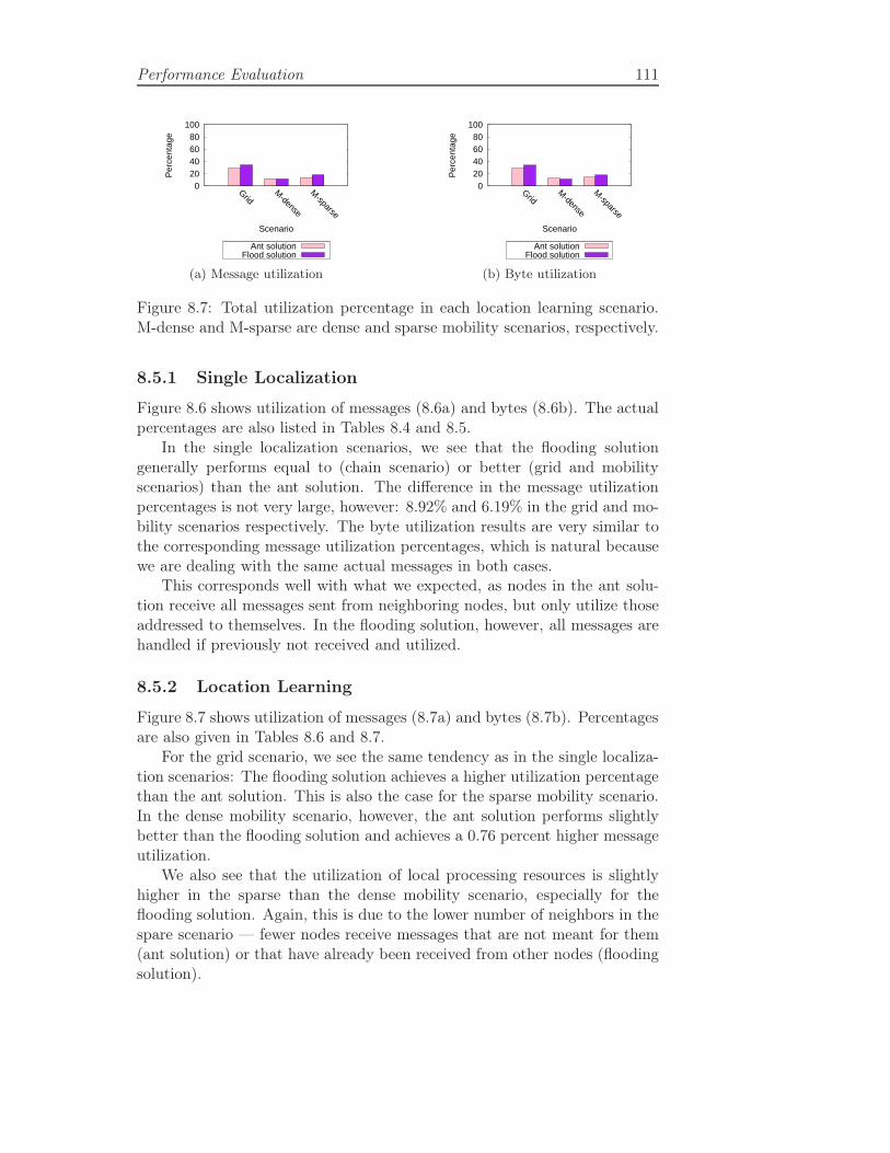
Performance Evaluation 111
0 20 40 60 80
100
GridM
-dense
M-sparse
Per
cent
age
Scenario
Ant solutionFlood solution
(a) Message utilization
0 20 40 60 80
100
GridM
-dense
M-sparse
Per
cent
age
Scenario
Ant solutionFlood solution
(b) Byte utilization
Figure 8.7: Total utilization percentage in each location learning scenario.M-dense and M-sparse are dense and sparse mobility scenarios, respectively.
8.5.1 Single Localization
Figure 8.6 shows utilization of messages (8.6a) and bytes (8.6b). The actualpercentages are also listed in Tables 8.4 and 8.5.
In the single localization scenarios, we see that the flooding solutiongenerally performs equal to (chain scenario) or better (grid and mobilityscenarios) than the ant solution. The difference in the message utilizationpercentages is not very large, however: 8.92% and 6.19% in the grid and mo-bility scenarios respectively. The byte utilization results are very similar tothe corresponding message utilization percentages, which is natural becausewe are dealing with the same actual messages in both cases.
This corresponds well with what we expected, as nodes in the ant solu-tion receive all messages sent from neighboring nodes, but only utilize thoseaddressed to themselves. In the flooding solution, however, all messages arehandled if previously not received and utilized.
8.5.2 Location Learning
Figure 8.7 shows utilization of messages (8.7a) and bytes (8.7b). Percentagesare also given in Tables 8.6 and 8.7.
For the grid scenario, we see the same tendency as in the single localiza-tion scenarios: The flooding solution achieves a higher utilization percentagethan the ant solution. This is also the case for the sparse mobility scenario.In the dense mobility scenario, however, the ant solution performs slightlybetter than the flooding solution and achieves a 0.76 percent higher messageutilization.
We also see that the utilization of local processing resources is slightlyhigher in the sparse than the dense mobility scenario, especially for theflooding solution. Again, this is due to the lower number of neighbors in thespare scenario — fewer nodes receive messages that are not meant for them(ant solution) or that have already been received from other nodes (floodingsolution).

112 Chapter 8
8.5.3 Conclusion
The differences in local processing power utilization are not very large, andseem to decrease with the size of the network and number of neighbors. Thisis natural, as the number of flooded messages will increase drastically whenthe total number of nodes and the number of neighbors per node increases.Under such circumstances, it will be harder for the forward ant to actuallylocate the requested resource in a larger network, but the mere fact thatthe network grows will not have an impact on the utilization, but only thenumber of hops needed to localize a resource, and thus also the number ofsent and received messages. However, if the average number of neighborsper node increases, more messages will be unnecessarily overheard, loweringthe utilization.

Chapter 9
Conclusion and Further Work
”A conclusion is simply the place where someone got tired of
thinking.”
— Arthur Block
In this last chapter we provide a summary of this thesis and its contribu-tion. We also give a summary of the performance analysis and observationsdone during performance testing and analysis and discuss some possible so-lutions and improvements to some of the observed problems and flaws. Wealso take a step back and look at the entire process from beginning to end.At last, we look at how our work may be continued, both in terms of furthertesting, to learn more about the solution’s performance, as well as how thesolution may be extended.
9.1 Contribution
The purpose for this thesis has been to design and develop a system enablingnodes in need of a resource to autonomously localize this resource if presentwithin the same partition of a MANET. The system is proposed as a so-lution if no other framework for resource location information sharing anddissemination is present, and is thus a general-purpose solution, not tailoredto function with any specific applications. When a node in the MANETfinds that it needs a certain resource not present within the node itself, ituses our solution to issue a resource request. If the resource is present atsome node within the same network partition, the requesting node should,eventually, get a resource reply from this node.
The characteristics of MANETs make design and implementation harder,as one always needs to consider the low availability of resources, such asbandwidth and processing power, as well as the (possibly) ever-changing
114 Chapter 9
network topology. Our aim has thus been to develop a system that requiredas little of these resources as possible rather than lowering the system’sresponse time.
Our system should be able to function autonomously, and should thuspreserve the self-* properties, such as self-organizing, self-configuration, self-optimization, self-protection and self-healing. Systems with such character-istics have always existed in nature, and may be used as inspiration whendesigning computer systems. In this thesis we have looked at stigmergy —the foraging behavior of ants, who communicate indirectly with one anotherby leaving pheromone trails on the ground. These trails, together with thefact that ants tend to prefer paths with high pheromone concentration, areused to make most ants walk the same, most optimal path between theirnest and a food source when gathering food.
The difference between our system and ants, is that we want our artificialants to spread out through the network to be able to search every corner forthe requested resource. To do this, we have turned ants’ behavior around anddesigned a system using what we call opposite stigmergy. In this approach,instead of walking the most used, or most recently used, path from a resource-requesting node, we choose the least recently used path.
In addition to the ant solution, we have designed and developed a verysimple flooding-based solution. The goal for this solution is the same asfor the ant solution: To localize a given resource — if present — withinthe MANET partition. However, the characteristics of flooding makes thisapproach behave and perform quite different from the ant approach. Whatwe expected was low response times but high resource usage. The aim ofthis solution was to provide alternative performance results for comparisonwith the ant solution.
We have tested our two solutions in a range of test scenarios and analyzedtheir performance in terms of response time, bandwidth usage and localprocessing power usage and utilization.
9.2 Performance Evaluation
The ant solution is designed according to two requirements. The first is anabsolute requirement:
• If a requested resource is present within the network, it must eventuallybe found.
The other requirement reflects the desired performance and relates to theenvironment in which the solution is designed to run, namely MANETs:
• The solution should consume as little resources, network wide as wellas node local, on one resource localization.

Conclusion and Further Work 115
• The solution should have a good resource utilization, both with respectto transmissions and local processing power.
Although low response time is also an advantage, this is, because of MANETcharacteristics, considered less important than good resource utilization.
Metrics were developed according to these requirements, and all resultsfrom the ant solution have been compared to the corresponding results fromthe flooding solution to see if the ant solution is actually worth using overother, simpler solutions.
From our test results we see that in many cases, the flooding solutionboth has a lower response time as well as a lower resource usage. However,we also see that when introducing more than one resource-requesting node,both the response time and the number of sent and received messages forthe ant solution decreases drastically. As expected, the ant solution didnot perform better than the flooding solution in any of the response timetest cases, but some of this is due to the much larger amount of processingneeded on each node in the ant solution. Data structures and algorithms canprobably be optimized to lower this delay somewhat, but there will always bea need for more extensive processing in the ant solution than in the floodingsolution.
If we look at the number of messages sent (bandwidth usage) and received(local processing power usage) in the two location learning test scenarios, wesee that the ant solution outperforms the flooding solution, thus, in numberof messages, we have managed to get a lower resource usage than that ofa flooding system, which was our primary goal. If we measure in numberof bytes, however, the large size of the virtual ants makes the ant solutionperform worse than the flooding solution. Again, it it possible to optimizethe data structures used, and thus lowering the amounts of bytes sent andreceived. As stated in Section 8.2.3, this also tells us that our time to live-limit was too high — using a lower limit might have helped, but might ofcourse also cause the need of more tries to be able to locate a resource. Thus,more tests are needed to figure out how small we may set this value withoutintroducing this new problem instead.
From the mobility scenario test cases, we also learned that a too highnumber of neighboring nodes makes it too hard for the ant to choose the”correct” way — it needs too many tries to choose the set of neighbors thatactually leads to the resource.
9.3 Critical Assessments
When we first started the work with this thesis, a lot of time was spentsearching for information regarding similar work. A lot of information isavailable on how stigmergy may be used for routing, both in traditional,

116 Chapter 9
wired networks as well as in MANETs, and also for a handful of other prob-lems related to optimization.
In the beginning, we imagined that our approach would be fairly simi-lar to the existing ACO approaches. The deeper into the problem we dove,however, the more we realized that our problem was, in some senses, funda-mentally different from that of the algorithms and approaches we had studiedto gather background information. We realized that what we were lookingfor was the opposite of anything we had seen — we wanted our artificial antsto spread throughout the network, not to gather themselves on one path. Insome areas, this lead to a lot of thinking, experimenting, failing and morethinking, whereas in other areas, it simplified things a lot. For example, ourpheromones are, at least at this stage, reduced to a timestamp, providingbuilt-in pheromone evaporation. The hardest part was thus in many casesto realize the solutions and to see, and also to accept, their simplicity, notthe actual implementation of the system.
The test setup and actual test phases were cumbersome. The lack of ex-perience with emulators such as NEMAN, together with a somewhat unrulytest computer, slowed the process down a bit, but we did manage to runthe most important test cases, although we would have liked to get a morecomplete set of test results.
We see from our performance analysis that there are a handful of thingsthat probably could have been done better another way. We also see thatour results do not paint the whole picture — more tests are needed to clarifyexactly which scenarios may benefit from our solution and which will proba-bly not. However, we do see a clear tendency and a potential that in certainscenarios and under certain circumstances, an ant approach to the resourcelocalization problem in MANETs is feasible.
Had we known when we started what we know now, a lot of problemsand design choices would obviously have been a lot easier and less timeconsuming. However, this is part of the process: Designing, implementing,testing, analyzing and then starting all over again, trying to address theproblems discovered when analyzing.
9.4 Further Work
9.4.1 Resource Localization in Sparse Networks
The solution developed in this thesis only works for dense networks, i.e.consisting of one partition only. However, MANETs are often sparse. Insome situations, the network may consist of more than one partition. Oursolution will then only search for a requested resource within the partitioncontaining the requesting node.
If a resource satisfying the demand is located within the partition, thereis probably no reason to start searching in other partitions. It is probably

Conclusion and Further Work 117
much easier for the requesting node to utilize the resource if it is located inthe same partition. However, the requesting node may be able to adapt ifthe only available resource is located in another partition, for example bymoving to that partition itself, or by utilizing delay tolerant techniques asdescribed in Section 2.1.3.
A natural expansion of our system is thus to enable searching in otherpartitions. To do this, we need a way to get the request and any replies toother partitions and back. We imagine an approach inspired by for exampleepidemic routing, where nodes could carry forward ants for a while, and ifno corresponding backward ant is received, the request could be forwardedif the node should meet new nodes. The difficult part here is figuring outwhich new nodes to forward the request to and not, as it is not necessary toforward the request to nodes in the same partition as the requesting node.Also, we need a way to stop the whole process if a resource is found, whichis difficult when nodes in several partitions may be working on solving thesame problem, but are unable to (easily) communicate with each other.
9.4.2 Resource Goodness
The existing solution does not differ between resource qualities as long asthey fulfill the demands of the requesting node. The ”goodness” of a resourcecan reflect the quality measurement of the resource, but also for examplehow close to the requesting node the resource holder is currently placed, howstable the resource is, both in terms of resource concentration (if appropriatefor the given resource), node mobility and node up-time, or perhaps the load,both on the path between requesting and holding nodes and on the actualresource on the holding node. If several nodes hold the requested resource,it might thus be good to locate several resource-holding nodes and pick theone that best satisfies the needs of the requesting node.
Locating several resources will put a higher load on the network, andshould thus only be done in MANETs that can deal with this extra cost.However, choosing for example the resource-holding node closest to the re-questing node might save resources if the requesting node decides to actuallyutilize the located resource in some way.
If we introduce some sort of goodness, this needs to be reflected in thepheromone values, so that subsequent ants can use this information whenlooking for a given resource. As mentioned in Section 5.5.5, there is a funda-mental difference in the information given by our pheromone values and theinformation provided by a goodness value: A goodness value is informationon a resource that has actually been localized, whereas our pheromone valuesprovide information about where ants have looked for a resource. One thusneeds to find a way to combine these two values.
One should also consider keeping track of every located resource, notonly the best like the current solution does. It is then possible to for example

118 Chapter 9
return the lowest quality matching resource if several are available, savingbetter resources for those that actually demand such high quality.
9.4.3 Further Implementation, Testing and Analysis
The tests and analyses from Chapter 8 give an indication of how the antsolution works, but are not enough to finally conclude on the performanceof the system. More tests are needed, and in addition to this, from theperformance analysis we have learned a few things about which changesshould be made to the system in order to increase its performance.
• In our grid and mobility scenarios, there are 25 nodes, one of whichis the node holding the requested resource. The very low resourcedensity makes the probability that an ant stumbles upon this nodequite low — the ant needs quite a bit of luck to locate the resource.This is reflected by our test results, where we see that a forward antneeds a very high number of hops to locate a resource in the two largerscenarios. More resource-holding nodes increases the possibility that aforward ant stumbles upon a satisfying resource. Tests should thus beperformed with more than one resource-holding node to see how thisimpacts the performance of the system.
• There are several parameters that may be tuned to the network charac-teristics, such as forward ant time to live-values and sleep time betweentwo subsequent forward ants. Extensive testing may be needed to findout the best ways to set these values. For example, it might be a goodidea to start with a quite low time to live-value, and if no resource islocated, increase this value incrementally until a resource is found.
• As stated in Section 8.3.3, one should consider allowing loops to get abetter resource location information dissemination. An alternative isallowing for example loops up to a certain length to avoid wasting toomuch resources on very long loops.
• Tests should be performed to see how many neighbors nodes may haveon average before this lowers the system performance.
• We should consider keeping pheromone lists for a neighbor for a whileafter it is lost in case it comes back.
• Implement an alternative ant solution which combines a reactive andproactive approach to scheduling as explained in Section 5.5.1.
• We should consider making the ant solution more robust to trans-mission errors, as explained in Section 8.1.1. However, if such errorhandling introduces too much overhead to the system, it might be best

Conclusion and Further Work 119
to skip this. As long as the resource-requesting node does not get abackward ant back, it will continue searching, so the resource will stilleventually be found. Whether this should be handled or not also de-pends on the level of mobility in the MANET — with relatively lownode mobility, the chance of sending a forward ant to a very recentlylost neighbor is quite small.

Bibliography
[1] olsrd - an adhoc wireless mesh routing daemon. Available [online]http://www.olsr.org/ (Retrieved 22.03.2010).
[2] TCPDUMP/LIBCAP public repository. Available [online] http://www.tcpdump.org/ (Retrieved 22.03.2010).
[3] Christian Blum and Xiaodong Li. Swarm intelligence in optimization. InChristian Blum and Daniel Merkle, editors, Swarm Intelligence, NaturalComputing Series, pages 43–85. Springer, 2008.
[4] G. Di Caro and M. Dorigo. Antnet: Distributed stigmergetic controlfor communications networks. J. Artif. Intell. Res. (JAIR), 9:317–365,1998.
[5] Gianni Di Caro, Frederick Ducatelle, and Luca Maria Gambardella.Swarm intelligence for routing in mobile ad hoc networks. In In Pro-ceedings of the 2005 IEEE Swarm Intelligence Symposium (SIS, 2005.
[6] Daily News From Cornell University Cornell Chronicle Online.Chemical helps ants remember where they left their food, showspromise for alzheimer’s disease, cornell scientists report, 1998.Available [online] http://www.news.cornell.edu/releases/Feb98/
antpheromone.hrs.html (Retrieved 31.03.2010).
[7] A. K. Dey. Understanding and using context. Personal UbiquitousComputing, 5(1):4–7, 2001.
[8] Gianni Di Caro, Frederick Ducatelle, and Luca Maria Gambardella.Anthocnet: an ant-based hybrid routing algorithm for mobile ad hocnetworks. In Parallel Problem Solving from Nature - PPSN VIII, volume3242 of LNCS, pages 461–470, Birmingham, UK, 18-22 September 2004.Springer-Verlag.
[9] M. Dorigo, E. Bonabeau, and G. Theraulaz. Ant algorithms and stig-mergy. Future Gener. Comput. Syst., 16(9):851–871, 2000.
[10] Marco Dorigo and Thomas Stützle. Ant Colony Optimization. The MITPress, 2004.

122 Bibliography
[11] Thomas D. Dyer and Rajendra V. Boppana. A comparison of TCPperformance over three routing protocols for mobile ad hoc networks.In MobiHoc, pages 56–66. ACM, 2001.
[12] Erling Falck-Ytter. Brannen i majorstutunnelen. Available [on-line] http://arkiv.brannmannen.no/?cid=11&aid=44980/ (Retrieved04.03.2010).
[13] Laura Marie Feeney. A taxonomy for routing protocols in mobile adhoc networks. Technical Report T99-07, Swedish Institute of ComputerScience, November 1, 1999.
[14] Dina Q. Goldin and David Keil. Toward domain-independent formal-ization of indirect interaction. In WETICE, pages 393–394. IEEE Com-puter Society, 2004.
[15] Marc Greis. Marc greis’ tutorial for the UCB/LBNL/VINT net-work simulator ”ns”, Chapter XI: Generating traffic-connection andnode-movement files for large wireless scenarios. Available [on-line] http://www.isi.edu/nsnam/ns/tutorial/nsscript7.html (Re-trieved 24.03.2010).
[16] International Organization for Standardization. Programming Language– C. ISO/IEC 9899.
[17] R. Jain. The Art of Computer Systems Performance Analysis. JohnWiley & Sons, Inc., New York, NY, 1991.
[18] David B. Johnson and David A. Maltz. Dynamic source routing in adhoc wireless networks. In Mobile Computing, pages 153–181. KluwerAcademic Publishers, 1996.
[19] Philo Juang, Hidekazu Oki, Yong Wang, Margaret Martonosi, Li-ShiuanPeh, and Daniel Rubenstein. Energy-efficient computing for wildlifetracking: design tradeoffs and early experiences with zebranet. In AS-PLOS, pages 96–107, 2002.
[20] J. O. Kephart and D. M. Chess. The vision of autonomic computing.IEEE Computer, 36(1):41–50, 2003.
[21] B. W. Kernighan and D. M. Ritchie. The C Programming Language,2nd edition. Prentice-Hall, 1988.
[22] Priya Mahadevan, Adolfo Rodriguez, David Becker, and Amin Vahdat.Mobinet: a scalable emulation infrastructure for ad hoc and wirelessnetworks. In WiTMeMo ’05: Papers presented at the 2005 workshop onWireless traffic measurements and modeling, pages 7–12, Berkeley, CA,USA, 2005. USENIX Association.
Bibliography 123
[23] S. Mehfuz and M. N. Doja. Swarm intelligent power-aware detection ofunauthorized and compromised nodes in manets. J. Artif. Evol. App.,2008:1–16, 2008.
[24] Sze-Yao Ni, Yu-Chee Tseng, Yuh-Shyan Chen, and Jang-Ping Sheu. Thebroadcast storm problem in a mobile ad hoc network. In MobiCom ’99:Proceedings of the 5th annual ACM/IEEE international conference onMobile computing and networking, pages 151–162, New York, NY, USA,1999. ACM.
[25] Hean Kuan Ong, Hean Loong Ong, Elok Robert Tee, andR. Sureswaran. Scalability study of ad-hoc wireless mobile network rout-ing protocol in sparse and dense networks. In Distributed Frameworksfor Multimedia Applications, 2006. The 2nd International Conferenceon, pages 1 –8, may 2006.
[26] Grassé P. La reconstruction du nid et les coordinations inter-individuelles chez Bellicostitermes natalensis et Cubitermes sp. Lathéorie de la stigmergie: Essai d’interpretation du comportement destermites constructeurs. Insectes Sociaux, 6:41–81, 1959.
[27] Margie Patlak, Thomas Baker, May Berenbaum, Ring Cardé, ThomasEisner, Jerrold Meinwald, Wendell Roelofs, and David Wood. Insectpheromones: Chemicals of communication. Beyond Discovery, 2003.
[28] J. Postel. RFC 768: User datagram protocol, August 1980.
[29] J. Postel. RFC 793: Transmission control protocol, September 1981.
[30] Matija Pužar. Towards Secure and Reliable Information Sharing inEmergency and Rescue Operations. PhD thesis, University of Oslo,2010.
[31] Matija Pužar and Thomas Plagemann. NEMAN: A network emulatorfor mobile ad-hoc networks. Technical report, Department of Informat-ics, University of Oslo, 2005.
[32] David Rising. Battlefield internet helps forces in iraq, April 2003.Available [online] http://www.redorbit.com/news/technology/
705/battlefield_internet_helps_forces_in_iraq/index.html
(Retrieved 04.03.2010).
[33] Elva J.H. Robinson, Duncan Jackson, Mike Holcombe, and Francis L.W.Ratnieks. Insect communication: ’no entry’ signal in ant foraging. Na-ture, 438(7067):443, 11 2005.

124 Bibliography
[34] S. Schmid, M. Sifalakis, and D. Hutchison. Towards autonomic net-works. In Autonomic Networking, First International IFIP TC6 Confer-ence, AN 2006, Paris, France, September 27-29, 2006, Proceedings, vol-ume 4195 of Lecture Notes in Computer Science, pages 1–11. Springer,2006.
[35] G. Di Marzo Serugendo, J. Fitzgerald, A. Romanovsky, and N. Guelfi.Dependable self-organising software architectures - an approach for self-managing systems. Technical report, School of Computer Science andInformation Systems, Birkbeck College, London, 2006.
[36] G. Di Marzo Serugendo, M. P. Gleizes, and A. Karageorgos. Self-organisation and emergence in MAS: An overview. Informatica (Slove-nia), 30(1):45–54, 2006.
[37] M. Sloman. Policy driven management for distributed systems. Journalof Network and Systems Management, 2:333, 1994.
[38] Jun-Zhao Sun. Mobile ad hoc networking: An essential technology forpervasive computing. In Proc. International Conferences on Info-tech& Info-net, Beijing, China.
[39] A. Toninelli. Semantic-Based Middleware Solutions to Support Context-Aware Service Provisioning in Pervasive Environments. PhD thesis,Università di Bologna, 2008.
[40] USC/ISI UC Berkeley, LBL and Xerox PARC. The network simulator- ns-2. Available [online] http://www.isi.edu/nsnam/ns/ (Retrieved06.04.2010).
[41] Amin Vahdat and David Becker. Epidemic routing for partially-connected ad hoc networks, May 08 2000.
[42] Tristram D. Wyatt. Pheromones and Animal Behaviour: Communica-tion by Smell and Taste. Cambridge University Press, 2003.
[43] Xiang Zeng, Rajive Bagrodia, and Mario Gerla. Glomosim: a libraryfor parallel simulation of large-scale wireless networks. SIGSIM Simul.Dig., 28(1):154–161, 1998.
[44] Wenrui Zhao, Mostafa H. Ammar, and Ellen W. Zegura. A messageferrying approach for data delivery in sparse mobile ad hoc networks.In Jun Murai, Charles E. Perkins, and Leandros Tassiulas, editors, Mo-biHoc, pages 187–198. ACM, 2004.
[45] Jim Zyren and Al Petrick. IEEE 802.11 Tutorial, 2002.Available [online] http://www.techonline.com/learning/techpaper/193101922 (Retrieved 04.03.2010).

Appendices


Appendix A
A Sample Scenario File
This chapter provides a quite simple sample scenario file. The differentcomponents of the scenario file is explained in comments within the file.Please note that, for aesthetic purposes, some lines have been split. This,however, would not be accepted by NEMAN.
A.1 Chain Scenario
The following is a simple chain scenario file where the node with IP address10.0.0.1, port 3457, is instructed to search for a resource with name memoryand quality 90 at 10 seconds into the emulation.
## nodes : 5 , pause : 0 . 00 , max speed : 0 . 00 ,
max x : 300 .00 , max y : 300 .00#
# Set node l o c a t i o n s :$node_ (0) s e t X_ 10.000000000000$node_ (0) s e t Y_ 10.000000000000$node_ (0) s e t Z_ 0.000000000000$node_ (1) s e t X_ 60.000000000000$node_ (1) s e t Y_ 10.000000000000$node_ (1) s e t Z_ 0.000000000000$node_ (2) s e t X_ 110.000000000000$node_ (2) s e t Y_ 10.000000000000$node_ (2) s e t Z_ 0.000000000000$node_ (3) s e t X_ 160.000000000000$node_ (3) s e t Y_ 10.000000000000$node_ (3) s e t Z_ 0.000000000000$node_ (4) s e t X_ 210.000000000000$node_ (4) s e t Y_ 10.000000000000

128 Appendix A
$node_ (4) s e t Z_ 0.000000000000
# Set which nodes are with in range o f each other :
$god_ set−d i s t 0 1 1$god_ set−d i s t 1 2 1$god_ set−d i s t 2 3 1$god_ set−d i s t 3 4 1
# Needed to make the t e s t l a s t f o r 20 seconds$ns_ at 20 .0 "$god_ set−d i s t 0 1 1"
# Send a reques t f o r r e s ource memory o f qua l i t y 3 to tap1 :$ns_ at 10.000000000000 "$node_ ( 1 0 . 0 . 0 . 1 )sendmsg port=3457 msg=’memory 3 ’"
# Set broadcas t range to get a# co r r e c t view in the NEMAN gui :# broadcast_range : 75 .00# data_range : 75 .00
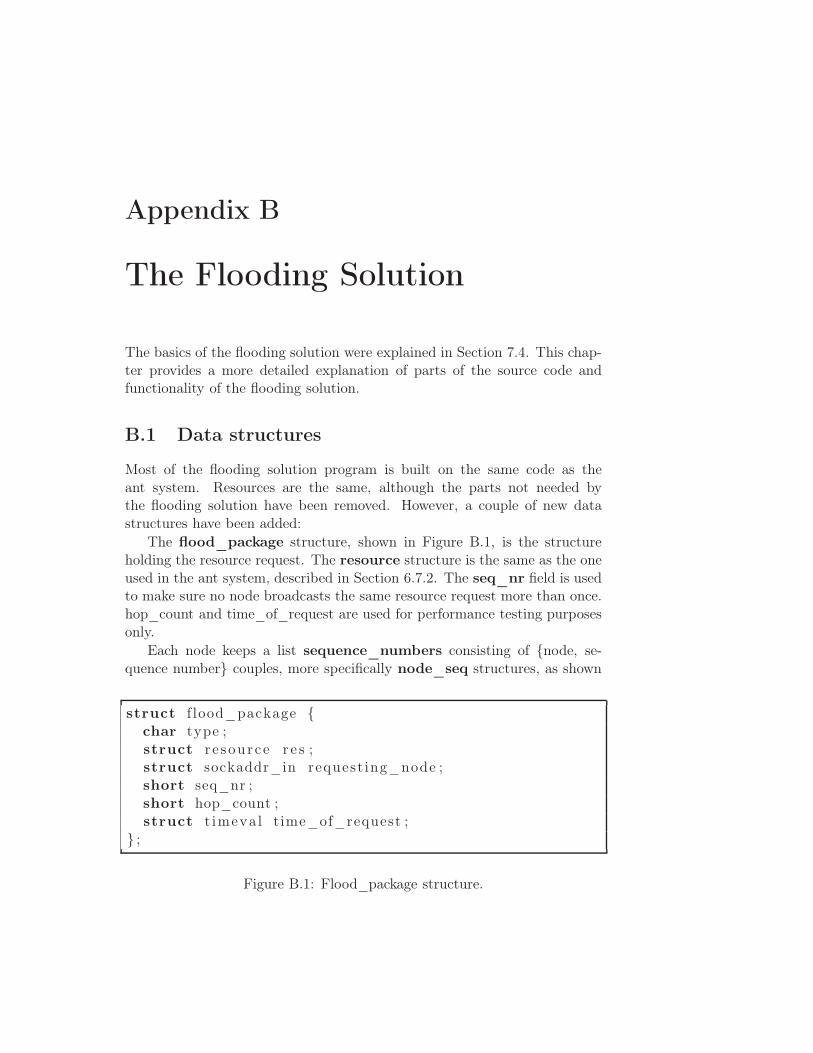
Appendix B
The Flooding Solution
The basics of the flooding solution were explained in Section 7.4. This chap-ter provides a more detailed explanation of parts of the source code andfunctionality of the flooding solution.
B.1 Data structures
Most of the flooding solution program is built on the same code as theant system. Resources are the same, although the parts not needed bythe flooding solution have been removed. However, a couple of new datastructures have been added:
The flood_package structure, shown in Figure B.1, is the structureholding the resource request. The resource structure is the same as the oneused in the ant system, described in Section 6.7.2. The seq_nr field is usedto make sure no node broadcasts the same resource request more than once.hop_count and time_of_request are used for performance testing purposesonly.
Each node keeps a list sequence_numbers consisting of {node, se-quence number} couples, more specifically node_seq structures, as shown
struct f lood_package {char type ;struct r e s ource r e s ;struct sockaddr_in request ing_node ;short seq_nr ;short hop_count ;struct t imeva l time_of_request ;
} ;
Figure B.1: Flood_package structure.

130 Appendix B
struct node_seq {struct sockaddr_in ∗node ;short highest_seen_seq ;
} ;
Figure B.2: Node_seq structure.
struct request_answer {char type ;struct r e s ource r e s ;struct sockaddr_in request ing_node ;
} ;
Figure B.3: Request_answer structure.
in Figure B.2. The list contains one entry for every other node this nodehas ever heard of and the highest seen sequence number for this node. Ifa request with sequence number less than or equal to this number for thecorresponding node, it is thrown away. If requests should, for some reason,appear out of order, this functionality may make a node throw away requeststhat should have been re-broadcast. In this very simple solution, however,we have chosen not to handle this, as this should not happen very often.
The last new structure is the request_answer structure, shown in FigureB.3. This structure is used for answers to requests.
B.1.1 Logging
Logging is done as in the ant solution, see Section 6.5 for details.
B.1.2 Program Flow
Threads
As the program should be able to manage several tasks at once, it is dividedinto several threads:
• The main process: Listens for incoming resource requests and resourcereplies.
• Thread 1: Listens for incoming resource requests. Created by the mainprocess shortly after startup.
• Thread 2: Initiates a resource search. Created by Thread 1 for everyincoming resource request.

Appendix C
Source Code
This chapter will go through some of the source code for the ant solution.
C.1 Program Layout — Ant Solution
The source code is divided into a number of files with respect to each func-tions purpose. These files are:
• main.c Initialization, reception of incoming resource requests and se-arch initiation.
• ant.[ch] The ant structure, all functions regarding ant sending, receiv-ing and handling.
• neighbor.[ch] The neighbor and neighbor_prob structures, topologyupdate reception and neighbor adding/deleting.
• resource.[ch] The resource and resource_info structures, resource in-formation registry and lookup.
• pheromone.[ch] The pheromone structure, building and updating ofpheromone lists.
• communication.[ch] All functions used to handle sockets, establish-ing connections and own address information retrieval.
• util.[ch] Type definitions and various utility functions, such as list op-erations, log file operations and uniformly distributed random numbergeneration.
C.2 Program Layout — Flooding Solution
This program is quite a bit smaller than the ant solution, but is still dividedinto several files:

132 Appendix C
• flood_main.c Initialization, reception of incoming resource requestsand search initiation.
• flood.[ch] The resource request and resource reply structures, all func-tions regarding request sending, receiving and handling.
• resource.[ch] The resource and resource_info structures, resource in-formation registry and lookup.
• communication.[ch] All functions used to handle sockets, establish-ing connections and own address information retrieval.
• util.[ch] Type definitions and various utility functions, such as listoperations and log file operations
Most of the code, unless the code in flood_main.c and flood.[ch] is moreor less identical to the corresponding ant solution code. Redundant functionsand variables have, however, been removed.
C.3 Building the Source Code
In addition to the source code, there are also makefiles (one for each solu-tion) which may be used to compile the source code. There are two optionswhen building the solution: Running make with the default target and withthe ”test” target. Building with the test target makes the system producean additional log file when run, namely the ant_test.log/flood_test.log file.This file is written to whenever a request for a resource either present at thereceiving node or with a known location is received. The information loggedincludes receiving node, requesting node, time spent on localization (in mil-liseconds, requiring synchronized clocks) and the number of hops traveled bythe forward ant/resource request, loops included.
C.4 Running the Source Code
The ant application may be run with the following command:
./ant <device> <ant_ttl> <max_sleep_time>
where device is the name of the network interface the program should use,ant_ttl is the number of hops one ant should be allowed to travel, andmax_sleep_time is the time one search may last before a new search isinitiated.
The flooding application is run with the following command:
./flood <device>
where device is the name of the network interface the program instanceshould use.

Appendix D
Code Examples
This chapter shows the source code of some of the most important parts ofthe ant solution, namely the sending and receiving of ants. Please note thatall code concerned with test information and debug information has beenleft out from this listing.
D.1 send_forward_ant()
send_forward_ant() is the function that is used to send forward ants fromneighbor to neighbor. It takes a ready made ant structure as argument,registers the requested resource in the list of all resources ever heard of,chooses a next hop neighbor and sends the forward ant there.
/∗ This func t ion takes a forward ant as argument , p i c k s a neighbor and∗ forwards the forward ant to t h i s neighbor ∗/
void send_forward_ant ( struct ant ∗ f_ant ){
int sock fd = get_unbound_udp_socket ( i f a c e ) ;
r e g i s t e r_re s ou r c e ( ( f_ant)−>re s ) ;
struct sockaddr_in ∗ ant_source = NULL;i f ( f_ant−>preceding_nodes > 0){
ant_source = ( struct sockaddr_in ∗) ( ( ( char ∗) f_ant )+ s izeof ( struct ant )+ ( f_ant−>preceding_nodes − 1)∗ s izeof ( struct sockaddr_in ) ) ;
}/∗ Find a neighbor to forward the ant to ∗/struct neighbor ∗n = get_neighbor (&((( struct ant ∗) f_ant)−>re s ) ,
ant_source ) ;i f (n == NULL){
f r e e ( f_ant ) ;c l o s e ( sock fd ) ;return ;
}struct sockaddr_in ∗ s i_des t = n−>si_n ;

134 Appendix D
memcpy(&f_ant−>next_hop , s i_dest , s izeof ( struct sockaddr_in ) ) ;s i_dest−>sin_port = htons ( a to i (ANT_PORT) ) ;
/∗ Calcu la t e s i z e o f new ant and forward ∗/int ant_size = s izeof ( struct ant )
+ ( ( struct ant ∗) f_ant)−>preceding_nodes∗ s izeof ( struct sockaddr_in ) ;
int s ent = sendto ( sockfd ,f_ant ,ant_size ,0 ,( struct sockaddr ∗) s i_dest ,( s izeof ( struct sockaddr_in ) ) ;
i f ( s ent == −1){
c l o s e ( sock fd ) ;f r e e ( f_ant ) ;return ;
}
c l o s e ( sock fd ) ;f r e e ( f_ant ) ;
}
D.2 receive_ants()
receive_ants() listens for incoming ants and calls new functions for furtherhandling:
/∗ This func t ion l i s t e n s f o r incoming ants ,∗ forward as we l l as backward ∗/
void ∗ rece i ve_ants ( ){
struct sockaddr_in s i_src ;s i ze_t addr_len = s izeof ( s i_s rc ) ;socklen_t ∗ __res tr i c t a l ;a l = ( socklen_t ∗)&addr_len ;
char ant [MAXANTLEN] ;
while (1){
int rv = recvf rom ( receive_ants_sockfd ,ant ,MAXANTLEN,0 ,( struct sockaddr ∗)& s i_src ,a l ) ;
i f ( rv == −1){
continue ;}
/∗ Check t ha t ant i s a c t u a l l y l a r g e enough∗ to contain an ant ∗/
struct ant ∗ rcvd_ant = ( struct ant ∗) ant ;i f ( rv >= s izeof ( struct ant ) &&

Code Examples 135
rv >= ( s izeof ( struct ant ) +rcvd_ant−>preceding_nodes ∗ s izeof ( struct sockaddr_in ) ) )
{/∗ Check i f ant was des t ined f o r t h i s node .
∗ Only needed during NEMAN emulation . ∗/i f ( rcvd_ant−>next_hop . sin_addr . s_addr !=
get_own_addr ( ) . sin_addr . s_addr ){
continue ;}
handle_received_ant ( rcvd_ant , s i_s rc ) ;}
}c l o s e ( rece ive_ants_sockfd ) ;
}
D.3 handle_received_ant()
handle_received_ant() is called by receive_ants(). It checks the typeof the incoming ant and calls functions for further handling based on the anttype. This function is also responsible for appending the address informationfor the last hop source to the forward ant (if the ant is actually a forwardant).
{/∗ This func t ion checks i f t he incoming ant was a forward or backward∗ ant , and c r ea t e s a new thread to f u r t he r handle the incoming ant ∗/
void handle_received_ant ( struct ant ∗ant_to_handle ,struct sockaddr_in s i_src )
{pthread_t t i d ;
i f ( ant_to_handle−>type == ’F ’ ){
/∗ Get new thread sa f e ant wi th updated address i n f o ∗/struct ant ∗ ts_f_ant =
( struct ant ∗) add_prev_address_info ( ant_to_handle , s i_s rc ) ;pthread_create(&tid , NULL, handle_forward_ant , (void ∗) ts_f_ant ) ;
}else i f ( ant_to_handle−>type == ’B ’ ){
/∗ Make t h r eadsa f e copy of the ant ∗/struct ant ∗ts_b_ant = mal loc ( s izeof ( struct ant )
+ ( ant_to_handle−>preceding_nodes∗ s izeof ( struct sockaddr_in ) ) ) ;
memcpy( ts_b_ant ,ant_to_handle ,
( s izeof ( struct ant ) + ( ant_to_handle−>preceding_nodes∗ s izeof ( struct sockaddr_in ) ) ) ) ;
pthread_create(&tid , NULL, handle_backward_ant , (void ∗) ts_b_ant ) ;}
}

136 Appendix D
D.4 handle_forward_ant()
handle_forward_ant() is called by handle_received_ant(). It checksif the requested resource is present. If not, it checks if any resource informa-tion for the requested resource is present. If not, the ant’s time to live valueis checked. If more hops are still allowed, send_forward_ant() is calledfor forwarding to a neighbor.
/∗ This f unc t i on t ak e s a forward ant as argument and checks i f∗ e i t h e r the reques t ed resource i s present , l o c a t i on informat ion∗ i s pre sent or the node should be forwarded to a neighbor ∗/
void ∗ handle_forward_ant (void ∗ant ){
struct ant ∗ f_ant = ( struct ant ∗) ant ;struct r e s ou r c e ∗ r e s = lookup_resource ( f_ant−>re s ) ;
i f ( r e s != NULL){
produce_backward_ant( res , f_ant ) ;f r e e ( r e s ) ;
}else
{struct r e s ou r c e ∗ r e s = lookup_resource_locat ion_info ( f_ant−>re s ) ;i f ( r e s != NULL){
produce_backward_ant( res , f_ant ) ;}else
{i f ( f_ant−>t t l == 1) /∗ No more hops a l lowed ∗/{
f r e e ( f_ant ) ;return NULL;
}/∗ Forward the forward ant to one neighbor ∗/send_forward_ant ( f_ant ) ;
}}return NULL;
}
D.5 handle_backward_ant()
handle_backward_ant() is called by handle_received_ants(). It ch-ecks whether the backward ant was a reply to itself or if it should be for-warded according to the address information in the ant.
void ∗ handle_backward_ant(void ∗ant ){
struct ant ∗ b_ant = ( struct ant ∗) ant ;r e g i s t e r_re s ou r c e_ l o ca t i on_ in f o (b_ant−>re s ) ;
i f (b_ant−>preceding_nodes == 0){
reg i s te r_resource_as_located (b_ant−>re s ) ;

Code Examples 137
}else
{/∗Forward ant according to ant informat ion ∗/forward_backward_ant ( b_ant ) ;
}return NULL;
}


Appendix E
CD Contents
This chapter describes the contents of the CD appended to this thesis. TheCD consists of three folders as described below.
E.1 /implementation
The implementation folder contains the C source code for both solutions.
E.1.1 /implementation/ant_solution
This folder contains the entire C code for the ant solution. The code isorganized as explained in Section C.1, and may be compiled as explained inSection C.3 and run as explained in Section C.4.
E.1.2 /implementation/flooding_solution
This folder holds the entire source code for the flooding solution. The organi-zation of the code is explained in Section C.2. The code is built as explainedin Section C.3 and run as explained in Section C.4.
E.2 /test_setup
The test_setup folder contains the tools used during the test phase. Theroot folder contains the following files:
• change_range.py: Removes all links with range 2 from a given sce-nario file, as explained in Section 7.8.2.
• delay_mobility.py: Delays all mobility in a given scenario file for 30seconds, as explained in Section 8.1.1.
• remove_links.py: Removes links from a given scenario file with aprobability of 0.7, as explained in Section 8.1.3.
140 Appendix E
• run_neman.sh: Runs a given scenario in NEMAN with the -no-guioption.
• run_nodes_ant.sh: Runs the ant solution with the given start andend nodes (tap device number), time to live value and max_sleep_time.
• run_nodes_flood.sh: Runs the flooding solution with the givenstart and end nodes (tap device number).
• run_tests.sh: Runs a complete set of tests for a given solution. Han-dles running of the three other run_*-scripts. Takes the following pa-rameters: number of repeated tests, name of scenario file, number ofnodes in scenario, name of output folder, and if ant solution also timeto live-value and max_sleep_time.
• tunnel.py: Needed when running emulations to tunnel control mes-sages from the NEMAN gui to the nodes.
E.2.1 /test_setup/scenarios
This folder contains the scenario files used during testing. The scenarios are:
• chain.sim: Chain scenario with one resource-requesting and one re-source-holding node.
• grid.sim: Grid scenario with one resource-requesting and one resour-ce-holding node.
• grid_3.sim: Grid scenario with three resource-requesting nodes andone resource-holding node.
• mobility.sim: Mobility scenario with one resource-requesting and oneresource-holding node.
• mobility_5_dense.sim: Dense mobility scenario with five resource-requesting nodes and one resource-holding node.
• mobility_5_sparse.sim: Sparse mobility scenario with five resour-ce-requesting nodes and one resource-holding node.
E.3 /analysis
The analysis folder contains the scripts used for analyzing the data outputfrom the tests. The following files were used:
• find_avg_hops.py: Parses a given <solution>.log file and prints theaverage number of hops and milliseconds used to localize a resource intests with only one resource-requesting node.

CD Contents 141
• multiple_find_avg_hops.py: Parses a given <solution>.log fileand prints the average number of hops and milliseconds per requestingnode used to localize a resource in tests with several resource-requestingnodes.
• find_connectivity.py: Parses a given scenario file and computes theadjacency matrix and average number of neighbors per node per secondinto the scenario. Output is written to a file, and each line of the fileis on the format ”time number_of_neighbors”.
• parse_tcpdump.py: Crawls the test output directory and parsesall nodes’ tcpdump files. Computes the number of sent and receivedmessages as well as the resource utilization.
The gnuplot-files for making plots from the output from these scripts arenot included.
