anova: analysis of variance - university of new...
TRANSCRIPT

Marc Mehlman
ANOVA: Analysis of Variance
Marc H. [email protected]
University of New Haven
“The analysis of variance is (not a mathematical theorem but) asimple method of arranging arithmetical facts so as to isolateand display the essential features of a body of data with theutmost simplicity.” – Sir Ronald A. Fisher
Marc Mehlman (University of New Haven) ANOVA: Analysis of Variance 1 / 31

Marc Mehlman
Table of Contents
1 ANOVA: One Way Layout
2 Comparing Means
3 ANOVA: Two Way Layout
4 Chapter #11 R Assignment
Marc Mehlman (University of New Haven) ANOVA: Analysis of Variance 2 / 31
Marc Mehlman
ANOVA (analysis of variance) is for testing if the means of k differentpopulations are equal when all the populations are independent, normaland have the same unknown variance.
An ANOVA test compares the randomness (variance) within groups(populations) to the randomness between groups. To test if the means ofall the populations are equal, one considers the ratio
variance between groups
variance within groups
as a test statistic. A large ratio would indicate a difference between inmeans between the groups.
Marc Mehlman (University of New Haven) ANOVA: Analysis of Variance 3 / 31

Marc Mehlman
ANOVA: One Way Layout
ANOVA: One Way Layout
ANOVA: One Way Layout
Marc Mehlman (University of New Haven) ANOVA: Analysis of Variance 4 / 31
Marc Mehlman
ANOVA: One Way Layout
7
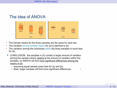
The sample means for the three samples are the same for each set. The variation among sample means for (a) is identical to (b). The variation among the individuals within the three samples is much less
for (b).
CONCLUSION: the samples in (b) contain a larger amount of variation among the sample means relative to the amount of variation within the samples, so ANOVA will find more significant differences among the means in (b)− assuming equal sample sizes here for (a) and (b).− Note: larger samples will find more significant differences.
The Idea of ANOVA
Marc Mehlman (University of New Haven) ANOVA: Analysis of Variance 5 / 31
Marc Mehlman
ANOVA: One Way Layout
Note:
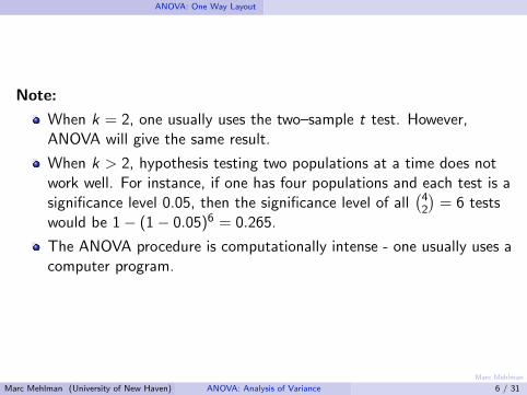
When k = 2, one usually uses the two–sample t test. However,ANOVA will give the same result.
When k > 2, hypothesis testing two populations at a time does notwork well. For instance, if one has four populations and each test is asignificance level 0.05, then the significance level of all
(42
)= 6 tests
would be 1− (1− 0.05)6 = 0.265.
The ANOVA procedure is computationally intense - one usually uses acomputer program.
Marc Mehlman (University of New Haven) ANOVA: Analysis of Variance 6 / 31

Marc Mehlman
ANOVA: One Way Layout
Assumptions for doing ANOVA
1 the populations are normal.
2 the populations have same (unknown) variance.
The above conditions are robust in the sense one can use ANOVA if thepopulations are approximately normal (otherwise the Kruskal–Wallis Test –a nonparametric test) and the population variances are approximatelyequal.
Convention: Rule for establishing equal variance
If the largest sample standard deviation is less than twice the smallestsample standard deviation, one can use ANOVA techniques under theassumption the variances are all the same.
Some textbooks use four times the smallest sample variance instead of justtwice.
Marc Mehlman (University of New Haven) ANOVA: Analysis of Variance 7 / 31

Marc Mehlman
ANOVA: One Way Layout
The Treatment or Factor is what differs between populations.
Example
A Blood pressure drug is administered to k populations in k differentdoses. One samples from each of the the k populations.
dosage #1 X11, · · · ,X1n1
......
dosage #k Xk1, · · · ,Xknk
Marc Mehlman (University of New Haven) ANOVA: Analysis of Variance 8 / 31
Marc Mehlman
ANOVA: One Way Layout
Definition
Let
kdef= # of levels (populations)
njdef= sample size of random sample from j th population
Ndef= n1 + n2 + · · ·+ nk = total number of random varibles
x̄jdef= sample mean from j th population
s2j
def= sample variance from j th population
x̄def= the grand mean =
1
N
k∑i=1
ni∑j=1
xij
Marc Mehlman (University of New Haven) ANOVA: Analysis of Variance 9 / 31
Marc Mehlman
ANOVA: One Way Layout
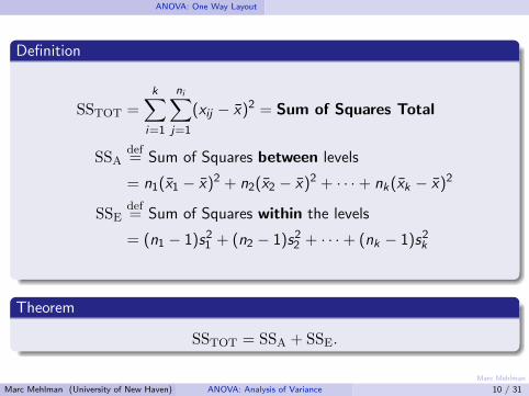
Definition
SSTOT =k∑
i=1
ni∑j=1
(xij − x̄)2 = Sum of Squares Total
SSAdef= Sum of Squares between levels
= n1(x̄1 − x̄)2 + n2(x̄2 − x̄)2 + · · ·+ nk(x̄k − x̄)2
SSEdef= Sum of Squares within the levels
= (n1 − 1)s21 + (n2 − 1)s2
2 + · · ·+ (nk − 1)s2k
Theorem
SSTOT = SSA + SSE.
Marc Mehlman (University of New Haven) ANOVA: Analysis of Variance 10 / 31
Marc Mehlman
ANOVA: One Way Layout
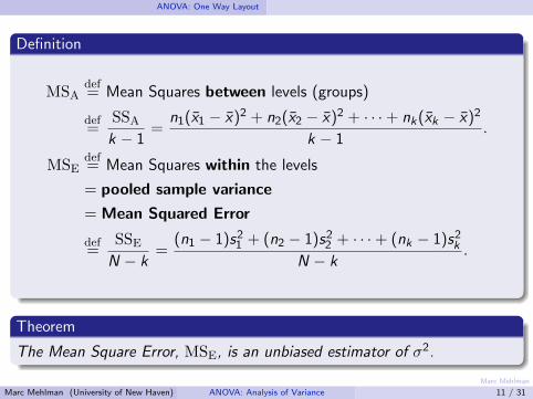
Definition
MSAdef= Mean Squares between levels (groups)
def=
SSAk − 1
=n1(x̄1 − x̄)2 + n2(x̄2 − x̄)2 + · · ·+ nk(x̄k − x̄)2
k − 1.
MSEdef= Mean Squares within the levels
= pooled sample variance
= Mean Squared Error
def=
SSEN − k
=(n1 − 1)s2
1 + (n2 − 1)s22 + · · ·+ (nk − 1)s2
k
N − k.
Theorem
The Mean Square Error, MSE, is an unbiased estimator of σ2.
Marc Mehlman (University of New Haven) ANOVA: Analysis of Variance 11 / 31

Marc Mehlman
ANOVA: One Way Layout
Theorem (ANOVA F Test)
To testH0 : µ1 = · · · = µk vs HA : not H0
use test statistic
F =MSAMSE
∼ F (k − 1,N − k) under H0.
Not H0 ⇒ F large, so use right tail test.
One creates an ANOVA table:
Source df SS MS F p
Between k − 1 SSA MSAMSAMSE
P(F(k − 1,N − I ) ≥ f )
Within N − k SSE MSE
Total N − 1 SSTOT
Marc Mehlman (University of New Haven) ANOVA: Analysis of Variance 12 / 31

Marc Mehlman
ANOVA: One Way Layout
Example
Judges at the Parisian photography contest, FotoGras, numerically scoredphotographs submitted by a number of photographers on a scale 0–10. AOne–Way Anova Test was performed to see which type of camera thephotograph was taken with had anything to do with the judges numericalscores. A summary of the data is given below:
Brand Sample Size Sample Mean Sample VarianceCanon 11 7.6 2.1Nikon 9 8.0 3.3Pentax 5 8.7 2.9Samsung 3 8.3 2.0Sony 8 8.0 1.9
The scores awarded from each brand was verified as being (mostly)normally distributed and independent from the scores awarded from otherbrands.Create an ANOVA Table from the scores and decide whether there was no“brand effect” at a 0.05 significance level.
Marc Mehlman (University of New Haven) ANOVA: Analysis of Variance 13 / 31

Marc Mehlman
ANOVA: One Way Layout
Example (cont.)
Solution:Since the largest sample standard deviation,
√3.3, is less than twice the size of the smallest sample variance,
√1.9, we can
assume the population variances are all the same.
k = 5
N = 11 + 9 + 5 + 3 + 8 = 36
x̄ =11(7.6) + 9(8.0) + 5(8.7) + 3(8.3) + 8(8.0)
36= 8.0
SSA = 11(7.6− 8.0)2 + 9(8.0− 8.0)2 + 5(8.7− 8.0)2 + 3(8.3− 8.0)2 + 8(8.0− 8.0)2 = 4.48
SSE = (11− 1)2.1 + (9− 1)3.3 + (5− 1)2.9 + (3− 1)2.0 + (8− 1)1.9 = 76.3
SSTOT = SSG + SSE = 4.48 + 76.3 = 80.78
MSA =SSA
k − 1=
4.48
5− 1= 1.12
MSE =SSE
N − k=
76.3
36− 5= 2.46129
f =MSA
MSE
=1.12
2.46129= 0.4550459
p–value = P(F(4, 31) ≥ f ) = 0.7679706
Source df SS MS F pBetween 4 4.48 1.12 0.45505 0.76797Within 31 76.3 2.46129Total 35 80.78
One accepts the hypothesis that there is no “brand” effect.
Marc Mehlman (University of New Haven) ANOVA: Analysis of Variance 14 / 31
Marc Mehlman
ANOVA: One Way Layout
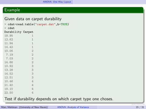
Example
Given data on carpet durability> cdat=read.table("carpet.dat",h=TRUE)
> cdat
Durability Carpet
18.95 1
12.62 1
11.94 1
14.42 1
10.06 2
7.19 2
7.03 2
14.66 2
10.92 3
13.28 3
14.52 3
12.51 3
10.46 4
21.40 4
18.10 4
22.50 4
Test if durability depends on which carpet type one choses.
Marc Mehlman (University of New Haven) ANOVA: Analysis of Variance 15 / 31
Marc Mehlman
ANOVA: One Way Layout
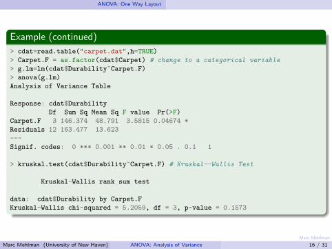
Example (continued)
> cdat=read.table("carpet.dat",h=TRUE)
> Carpet.F = as.factor(cdat$Carpet) # change to a categorical variable
> g.lm=lm(cdat$Durability~Carpet.F)
> anova(g.lm)
Analysis of Variance Table
Response: cdat$Durability
Df Sum Sq Mean Sq F value Pr(>F)
Carpet.F 3 146.374 48.791 3.5815 0.04674 *
Residuals 12 163.477 13.623
---
Signif. codes: 0 *** 0.001 ** 0.01 * 0.05 . 0.1 1
> kruskal.test(cdat$Durability~Carpet.F) # Kruskal--Wallis Test
Kruskal-Wallis rank sum test
data: cdat$Durability by Carpet.F
Kruskal-Wallis chi-squared = 5.2059, df = 3, p-value = 0.1573
Marc Mehlman (University of New Haven) ANOVA: Analysis of Variance 16 / 31

Marc Mehlman
Comparing Means
Comparing Means
Comparing Means
Marc Mehlman (University of New Haven) ANOVA: Analysis of Variance 17 / 31

Marc Mehlman
Comparing Means
If H0 is rejected, ie all means are not equal, how do you find how thepopulation means differ from each other?
Answer:
boxplots (all in one graph).
multiple comparison methods such as the Bonferroni MultipleComparison Test.
Marc Mehlman (University of New Haven) ANOVA: Analysis of Variance 18 / 31
Marc Mehlman
Comparing Means
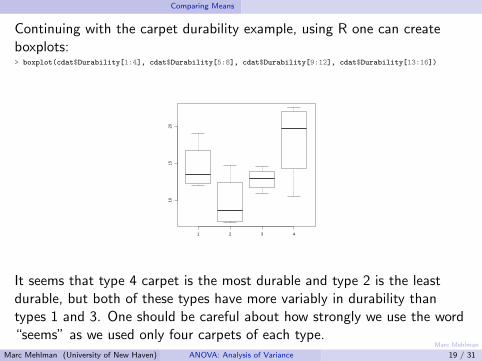
Continuing with the carpet durability example, using R one can createboxplots:> boxplot(cdat$Durability[1:4], cdat$Durability[5:8], cdat$Durability[9:12], cdat$Durability[13:16])
1 2 3 4
1015
20
It seems that type 4 carpet is the most durable and type 2 is the leastdurable, but both of these types have more variably in durability thantypes 1 and 3. One should be careful about how strongly we use the word“seems” as we used only four carpets of each type.
Marc Mehlman (University of New Haven) ANOVA: Analysis of Variance 19 / 31

Marc Mehlman
Comparing Means
Definition
A least significant differences (LDS) method is a multiple–comparisons procedurethat tests each pair of levels and rejects H0 : µ1 = · · · = µk if any of the
(k2
)tests is
significant.
The Bonferroni Multiple Comparison Test is a LDS method.
Theorem (Bonferroni Multiple Comparison Test)
To test H0 at the α significance level for every 1 ≤ i < j ≤ k:
Step #1 calculate the test statistic
tij =x̄j − x̄i√
MSE
(1ni
+ 1nj
) ∼ t(N − k).
Step #2 Test whether the means of levels i and j are equal at the α
(k2)level using
the a two–sided test with the test statistic tij .
If any of the(k2
)test are significant, reject H0. Otherwise accept H0.
Marc Mehlman (University of New Haven) ANOVA: Analysis of Variance 20 / 31

Marc Mehlman
Comparing Means
Example
> pairwise.t.test(cdat$Durability, Carpet.F, "bonferroni")
Pairwise comparisons using t tests with pooled SD
data: cdat$Durability and Carpet.F
1 2 3
2 0.564 - -
3 1.000 1.000 -
4 1.000 0.045 0.388
P value adjustment method: bonferroni
Marc Mehlman (University of New Haven) ANOVA: Analysis of Variance 21 / 31

Marc Mehlman
ANOVA: Two Way Layout
ANOVA: Two Way Layout
ANOVA: Two Way Layout
Marc Mehlman (University of New Haven) ANOVA: Analysis of Variance 22 / 31
Marc Mehlman
ANOVA: Two Way Layout
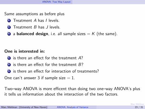
Same assumptions as before plus
1 Treatment A has I levels.
2 Treatment B has J levels.
3 a balanced design, i.e. all sample sizes = K (the same).
One is interested in:
1 is there an effect for the treatment A?
2 is there an effect for the treatment B?
3 is there an effect for interaction of treatments?
One can’t answer 3 if sample size = 1.
Two–way ANOVA is more efficent than doing two one–way ANOVA’s plusit tells us information about the interaction of the two factors.
Marc Mehlman (University of New Haven) ANOVA: Analysis of Variance 23 / 31
Marc Mehlman
ANOVA: Two Way Layout
Definition
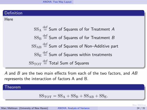
Here
SSAdef= Sum of Squares of for Treatment A
SSBdef= Sum of Squares of for Treatment B
SSABdef= Sum of Squares of Non–Additive part
SSEdef= Sum of Squares within treatments
SSTOTdef= Total Sum of Squares
A and B are the two main effects from each of the two factors, and ABrepresents the interaction of factors A and B.
Theorem
SSTOT = SSA + SSB + SSAB + SSE.
Marc Mehlman (University of New Haven) ANOVA: Analysis of Variance 24 / 31
Marc Mehlman
ANOVA: Two Way Layout
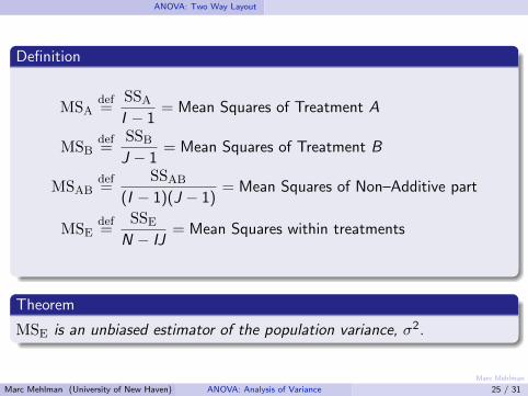
Definition
MSAdef=
SSAI − 1
= Mean Squares of Treatment A
MSBdef=
SSBJ − 1
= Mean Squares of Treatment B
MSABdef=
SSAB
(I − 1)(J − 1)= Mean Squares of Non–Additive part
MSEdef=
SSEN − IJ
= Mean Squares within treatments
Theorem
MSE is an unbiased estimator of the population variance, σ2.
Marc Mehlman (University of New Haven) ANOVA: Analysis of Variance 25 / 31
Marc Mehlman
ANOVA: Two Way Layout
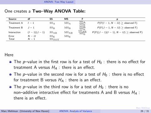
One creates a Two–Way ANOVA Table:
Source df SS MS F p
Treatment A I − 1 SSA MSAMSAMSE
P(F(I − 1,N − IJ) ≥ observed F)
Treatment B J − 1 SSB MSBMSBMSE
P(F(J − 1,N − IJ) ≥ observed F)
Interaction (I − 1)(J − 1) SSAB MSABMSABMSE
P(F((J − 1)(I − 1),N − IJ) ≥ observed F)
Error N − IJ SSE MSETotal N − 1 SSTOT
Here
The p–value in the first row is for a test of H0 : there is no effect fortreatment A versus HA : there is an effect.
The p–value in the second row is for a test of H0 : there is no effectfor treatment B versus HA : there is an effect.
The p–value in the third row is for a test of H0 : there is nonon–additive interactive effect for treatments A and B versus HA :there is an effect.
Marc Mehlman (University of New Haven) ANOVA: Analysis of Variance 26 / 31
Marc Mehlman
ANOVA: Two Way Layout
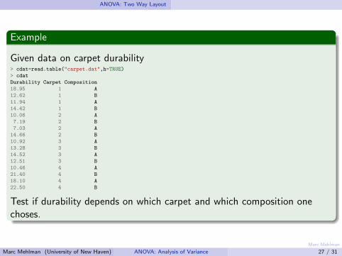
Example
Given data on carpet durability> cdat=read.table("carpet.dat",h=TRUE)
> cdat
Durability Carpet Composition
18.95 1 A
12.62 1 B
11.94 1 A
14.42 1 B
10.06 2 A
7.19 2 B
7.03 2 A
14.66 2 B
10.92 3 A
13.28 3 B
14.52 3 A
12.51 3 B
10.46 4 A
21.40 4 B
18.10 4 A
22.50 4 B
Test if durability depends on which carpet and which composition onechoses.
Marc Mehlman (University of New Haven) ANOVA: Analysis of Variance 27 / 31
Marc Mehlman
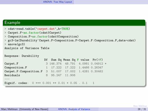
ANOVA: Two Way Layout
Example
> cdat=read.table("carpet.dat",h=TRUE)
> Carpet.F=as.factor(cdat$Carpet)
> Composition.F=as.factor(cdat$Composition)
> gc3=lm(Durability~Carpet.F+Composition.F+Carpet.F:Composition.F,data=cdat)
> anova(gc3)
Analysis of Variance Table
Response: Durability
Df Sum Sq Mean Sq F value Pr(>F)
Carpet.F 3 146.374 48.791 4.0981 0.04912 *
Composition.F 1 17.222 17.222 1.4466 0.26347
Carpet.F:Composition.F 3 51.007 17.002 1.4281 0.30462
Residuals 8 95.247 11.906
---
Signif. codes: 0 *** 0.001 ** 0.01 * 0.05 . 0.1 1
Marc Mehlman (University of New Haven) ANOVA: Analysis of Variance 28 / 31

Marc Mehlman
Chapter #11 R Assignment
Chapter #11 R Assignment
Chapter #11 R Assignment
Marc Mehlman (University of New Haven) ANOVA: Analysis of Variance 29 / 31
Marc Mehlman
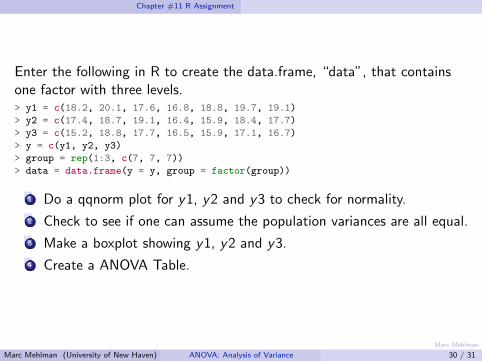
Chapter #11 R Assignment
Enter the following in R to create the data.frame, “data”, that containsone factor with three levels.> y1 = c(18.2, 20.1, 17.6, 16.8, 18.8, 19.7, 19.1)
> y2 = c(17.4, 18.7, 19.1, 16.4, 15.9, 18.4, 17.7)
> y3 = c(15.2, 18.8, 17.7, 16.5, 15.9, 17.1, 16.7)
> y = c(y1, y2, y3)
> group = rep(1:3, c(7, 7, 7))
> data = data.frame(y = y, group = factor(group))
1 Do a qqnorm plot for y1, y2 and y3 to check for normality.
2 Check to see if one can assume the population variances are all equal.
3 Make a boxplot showing y1, y2 and y3.
4 Create a ANOVA Table.
Marc Mehlman (University of New Haven) ANOVA: Analysis of Variance 30 / 31

Marc Mehlman
Chapter #11 R Assignment
The data file “data2way.csv”, found on
math.newhaven.edu/mhm/courses/bstat/items.html,
contains a hypothetical sample of 27 participants who are divided intothree stress reduction treatment groups (mental, physical and medical)and three age groups (young, mid, and old). The stress reduction valuesare represented on a scale that ranges from 0 to 10. Read this data into Rusingdata2way = read.csv("data2way.csv")
Create a two-way ANOVA table and use the table for the following fourproblems:
5 Consider a test that the treatments have no effect on stress versusthere is an effect. What is the p–value of this test.
6 Consider a test that age has no effect on stress versus there is aneffect. What is the p–value of this test.
7 What is SSTOT ?8 What is the degrees of freedom for SSTOT?
Marc Mehlman (University of New Haven) ANOVA: Analysis of Variance 31 / 31