anomalous and significant subgraph detection in attributed...
TRANSCRIPT

Anomalous and Significant Subgraph
Detection in Attributed Networks
Feng Chen 1, Petko Bogdanov 1, Daniel B. Neill 2, and
Ambuj K. Singh 3
1
Department of Computer Science
College of Engineering and Applied Sciences
University at Albany - SUNY
1
Event and Pattern Detection Laboratory
H.J. Heinz III College
Carnegie Mellon University
Department of Computer Science &
Biomolecular Science and Engineering
University of California at Santa Barbara
2
3

Roadmap
• Introduction and motivation
• Part 1: Subgraph detection in static
attributed networks
• Part 2: Subgraph detection in dynamic
attributed networks
• Conclusion and future directions
2
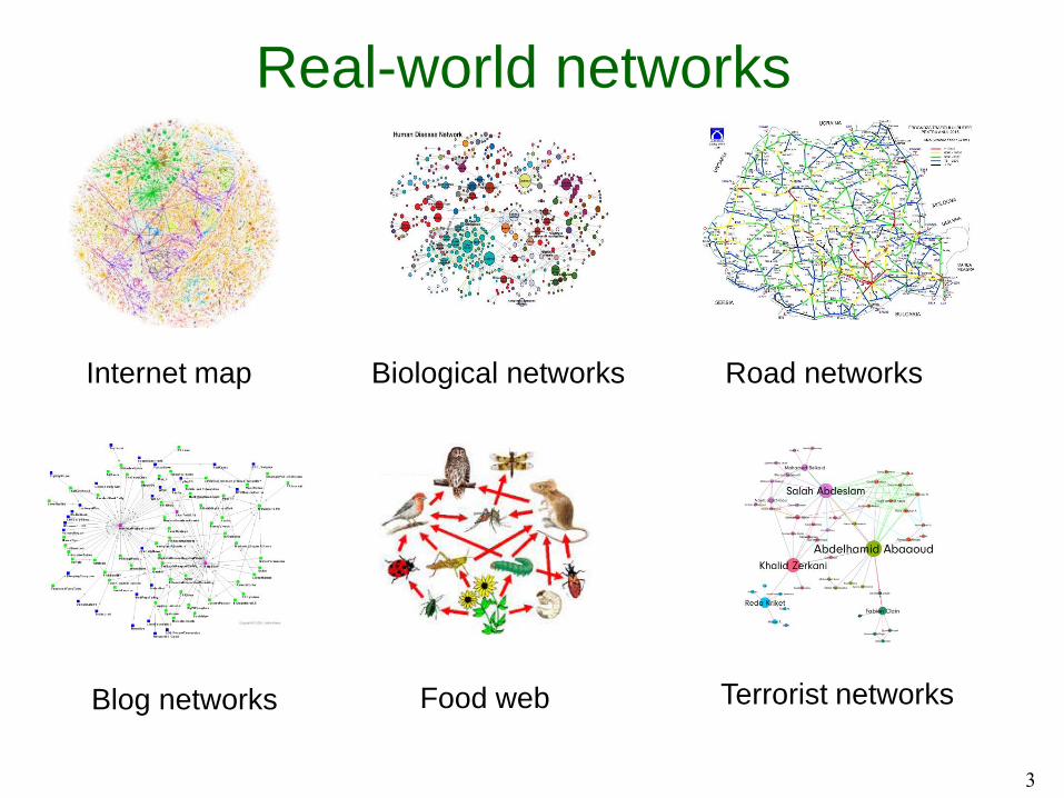
Real-world networks
3
Internet map
Food web Terrorist networksBlog networks
Biological networks Road networks

Real-world networks
4
Protein-protein
interaction networks
Retail networks Water distribution
networksFacebook friends’
networks
Power grid networks Dating networks

Anomalous and significant subgraphs refer
to subgraphs, in which the behaviors
(attributes) of the nodes or edges are
significantly different from the behaviors of
those outside the subgraphs.
5
Anomalous & significant subgraphs
This tutorial mainly reviews methods on
detection of anomalous and significant
subgraphs with connectivity constraint.

Anomalous & significant subgraphs
• Detection of subnetwork biomarkers
6
(Chuang et al. 2007)

Anomalous & significant subgraphs
7
• Detection of road traffic congestion events
https://mikethemadbiologist.com/2015/08/08/the-ripple-
effects-of-mass-transit/

Anomalous & significant subgraphs
• Detection of abnormally high breakage in a
distribution network
8
(de Oliveira et al., 2010)

Anomalous & significant subgraphs
9
• Detection of disease outbreaks
http://alfa-img.com/show/ebola-epidemic-map-2015.html

Other applications
10
Societal events in social media Malicious cargo
Image/video surveillance
Auction fraud, fake reviews, email spams, false advertising
New business discovery
Extreme weather events Crime hotspots
Brain activities Disease diagnosis Animal activities
New chemical structures New knowledge discovery

Subgraph detection: definition
• Univariate static networks
11
12
3
45
6 7
1 2 3 4 5 6 7
Network topology 𝔾 = 𝕍, 𝔼
Node ID
𝐹(𝑆) characterizes the
level of anomalousness
of S based on attributes.
Constraint is defined
based on network
topology.
Attributes (w)
max𝑆⊆𝕍
𝐹(𝑆)
𝑠. 𝑡. 𝑆 satisfies a predefinedtopological constraint (e.g.
connectivity).
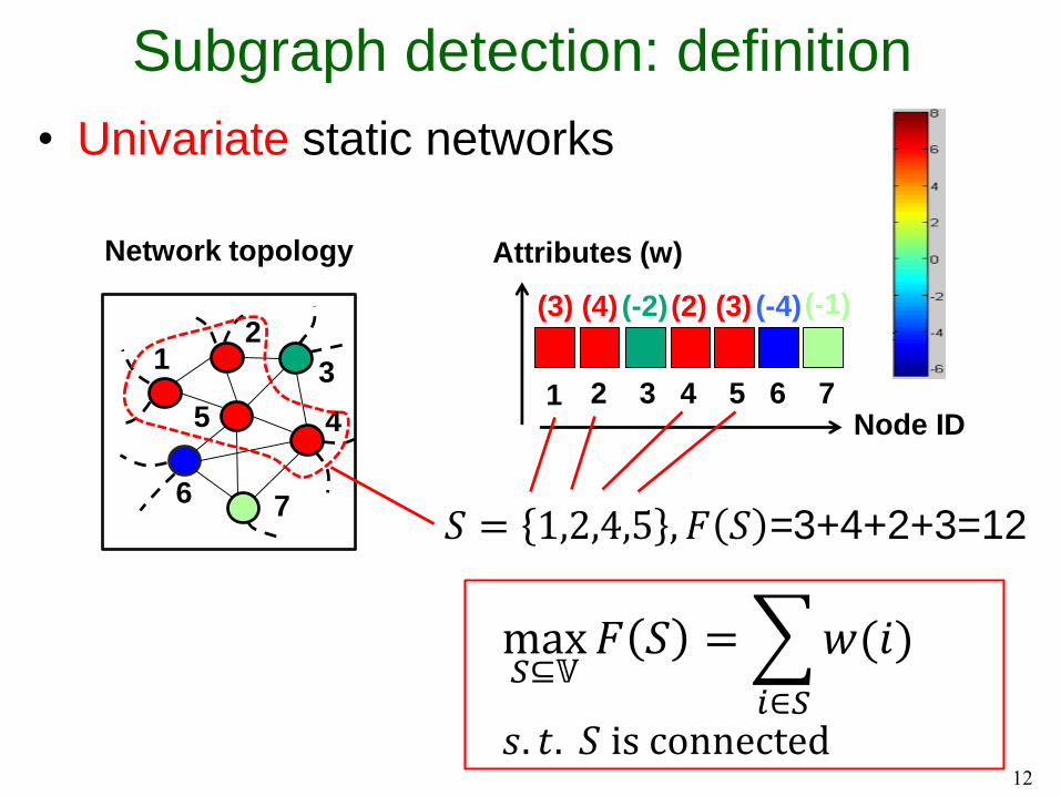
Subgraph detection: definition
• Univariate static networks
12
12
3
45
6 7
1 2 3 4 5 6 7
Network topology Attributes (w)
Node ID
(3) (4) (-2)(2) (3) (-4)(-1)
𝑆 = 1,2,4,5 , 𝐹 𝑆 =3+4+2+3=12
max𝑆⊆𝕍
𝐹 𝑆 =
𝑖∈𝑆
𝑤(𝑖)
𝑠. 𝑡. 𝑆 is connected

Subgraph detection: definition
• Multivariate static networks
13
12
3
45
6 7 1 2 3 4 5 6 7
Network topology
Node ID
Constraint is defined
based on network
topology.
Att
rib
ute
s (
w)
max𝑆,𝑅
𝐹(𝑆, 𝑅)
𝑠. 𝑡. 𝑆 satisfies a predefinedtopological constraint
𝑅=
1,2,4
𝑆 = 1,2,4,5

Subgraph detection: definition
• Multivariate static networks
14
12
3
45
6 7 1 2 3 4 5 6 7
Network topology
Node ID
Constraint is defined
based on network
topology.
Att
rib
ute
s (
w)
max𝑆,𝑅
𝐹(𝑆, 𝑅)
𝑠. 𝑡. 𝑆 satisfies a predefinedtopological constraint
𝑅=
1,2,4
𝑆 = 1,2,4,5

Subgraph detection: definition
• Multivariate static networks
15
12
3
45
6 7 1 2 3 4 5 6 7
Network topology
Node ID
Constraint is defined
based on network
topology.
Att
rib
ute
s (
w)
max𝑆,𝑅
𝐹(𝑆, 𝑅)
𝑠. 𝑡. 𝑆 satisfies a predefinedtopological constraint
𝑆 = 1,2,4,5
𝑅=
1,2,4

Subgraph detection: definition
• Multivariate dynamic networks
16
12
3
45
6 7 1 2 3 4 5 6 7
Network topology
Constraint is defined
based on network
topology.
Att
rib
ute
s
Nodes
max𝑆,𝑅,𝑊
𝐹(𝑆, 𝑅,𝑊)
𝑠. 𝑡. 𝑆 satisfies a predefinedtopological constraint

Subgraph detection: definition
17
12
3
45
6 7
Network topology
Constraint is defined
based on network
topology.
𝑆 = 1,2,4,5
Att
rib
ute
s
max𝑆,𝑅,𝑊
𝐹(𝑆, 𝑅,𝑊)
𝑠. 𝑡. 𝑆 satisfies a predefinedtopological constraint

Subgraph detection: definition
18
12
3
45
6 7
Network topology
Constraint is defined
based on network
topology.
max𝑆,𝑅,𝑊
𝐹(𝑆, 𝑅,𝑊)
𝑠. 𝑡. 𝑆 satisfies a predefinedtopological constraint
𝑆 = 1,2,4,5
𝑅=
1,2,4

Subgraph detection: definition
19
12
3
45
6 7
Network topology
Constraint is defined
based on network
topology.
max𝑆,𝑅,𝑊
𝐹(𝑆, 𝑅,𝑊)
𝑠. 𝑡. 𝑆 satisfies a predefinedtopological constraint
𝑆 = 1,2,4,5
𝑅=
1,2,4

Subgraph detection: definition
20
12
3
45
6 7
Network topology
Constraint is defined
based on network
topology.
max𝑆,𝑅,𝑊
𝐹(𝑆, 𝑅,𝑊)
𝑠. 𝑡. 𝑆 satisfies a predefinedtopological constraint
𝑆 = 1,2,4,5
𝑅=
1,2,4

Subgraph detection: definition
21
12
3
45
6 7
Network topology
Constraint is defined
based on network
topology.
max𝑆,𝑅,𝑊
𝐹(𝑆, 𝑅,𝑊)
𝑠. 𝑡. 𝑆 satisfies a predefinedtopological constraint
𝑆 = 1,2,4,5
𝑅=
1,2,4

Score function & constraints
• Score functions
• Parametric scan statistics
• Kulldorff’s statistic, Expectation-based statistic
• Nonparametric scan statistics
• Higher Criticism (HC) statistic, Berk-Jones’s statistic
• Network design based functions
• Prize Collecting Steiner Tree (PCST) objective
• Topological constraints
• Regular shapes, such as circles and rectangles.
• Connectivity (the focus of this tutorial)
• Compactness22

Computational Challenges
• Exponentially many possible subsets,
𝑂 2𝑁 ⋅ 2𝑀 , where 𝑁 and 𝑀 refer to the total
numbers of nodes and attributes,
respectively: computationally infeasible for
naïve search.
• Given a score function and a topological
constraint (e.g. connectivity) predefined by a
user, how we can identify the highest
scoring subgraphs efficiently and
effectively?
23
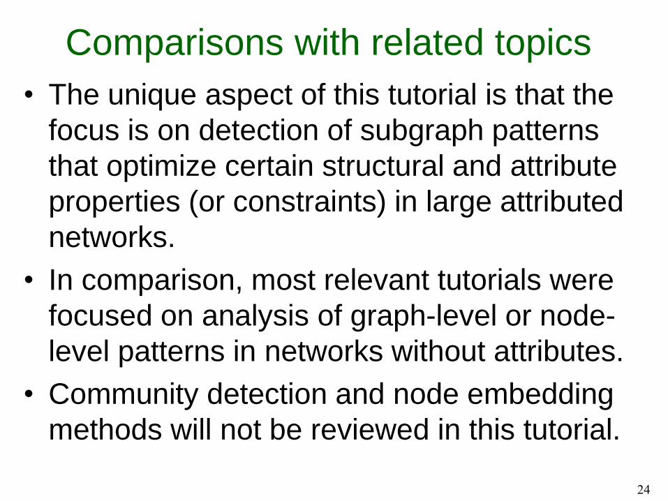
Comparisons with related topics
• The unique aspect of this tutorial is that the
focus is on detection of subgraph patterns
that optimize certain structural and attribute
properties (or constraints) in large attributed
networks.
• In comparison, most relevant tutorials were
focused on analysis of graph-level or node-
level patterns in networks without attributes.
• Community detection and node embedding
methods will not be reviewed in this tutorial.
24

Part 1: Subgraph Detection
in Static Attributed
Networks
25

Taxonomy
26
Anomalous & significant subgraph detection
Static attributed networks Dynamic attributed networks
Fast subset
scan
Complex networksSpatial networks
Graph
scan
Nonparametric
graph scan
Submodular
optimization
methods
Graph-structured
Sparse optimization
methods
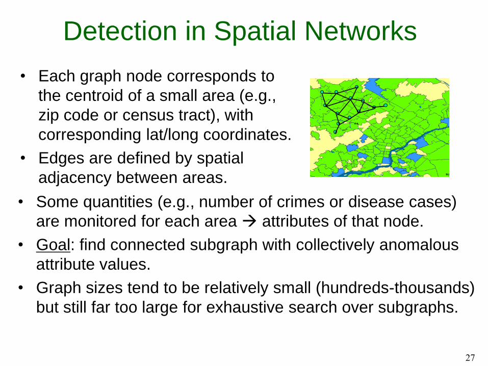
Detection in Spatial Networks
• Each graph node corresponds to
the centroid of a small area (e.g.,
zip code or census tract), with
corresponding lat/long coordinates.
• Edges are defined by spatial
adjacency between areas.
27
• Some quantities (e.g., number of crimes or disease cases)
are monitored for each area attributes of that node.
• Goal: find connected subgraph with collectively anomalous
attribute values.
• Graph sizes tend to be relatively small (hundreds-thousands)
but still far too large for exhaustive search over subgraphs.

28
Multivariate event detection
Spatial time series data from
spatial locations si (e.g. zip codes)
Time series of counts
ci,mt for each zip code si
for each data stream dm.
d1 = respiratory ED
d2 = constitutional ED
d3 = OTC cough/cold
d4 = OTC anti-fever
Outbreak detection
(etc.)
Main goals:
Detect any emerging events.
Pinpoint the affected subset of
locations and time duration.
Characterize the event by
identifying the affected streams.
Compare hypotheses:
H1(D, S, W)
D = subset of streams
S = subset of locations
W = time duration
vs. H0: no events occurring

29
Expectation-based scan statistics(Kulldorff, 1997; Neill and Moore, 2005)
We search for spatial regions
(subsets of locations) where the
recently observed counts for
some subset of streams are
significantly higher than expected.
Expected
counts
Historical
counts
Current counts
(3 day duration)
We perform time series analysis
to compute expected counts
(“baselines”) for each location and
stream for each recent day.
We then compare the actual and
expected counts for each subset
(D, S, W) under consideration.

30
We find the subsets with highest
values of a likelihood ratio statistic,
and compute the p-value of each
subset by randomization testing.
Maximum subset
score = 9.8
2nd highest
score = 8.4
Significant! (p = .013)
Not significant
(p = .098)
…
F1* = 2.4 F2* = 9.1 F999* = 7.0To compute p-value
Compare subset score
to maximum subset
scores of simulated
datasets under H0.
Expectation-based scan statistics(Kulldorff, 1997; Neill and Moore, 2005)
F(D,S,W ) =Pr(Data |H1(D,S,W ))
Pr(Data |H 0)

31
Which regions to search?Typical approach: “spatial scan” (Kulldorff, 1997)
Each search region S is a sub-region of space.• Choose some region shape (e.g. circles, rectangles) and
consider all regions of that shape and varying size.
• Low power for true events that do not correspond well to the chosen set of search regions (e.g. irregular shapes).
Our approach: “subset scan” (Neill, 2012)Each search region S is a subset of locations.
• Find the highest scoring subset, subject to some constraints (e.g. spatial proximity, connectivity).
• For multivariate, also optimize over subsets of streams.
• Exponentially many possible subsets, O(2N x 2M): computationally infeasible for naïve search.
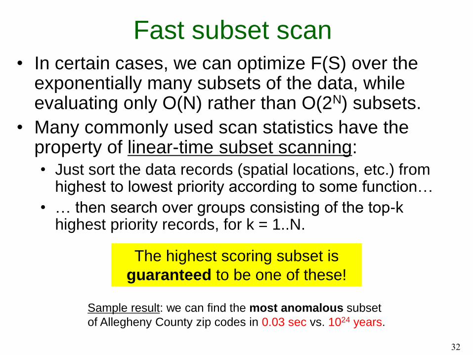
Fast subset scan• In certain cases, we can optimize F(S) over the
exponentially many subsets of the data, while evaluating only O(N) rather than O(2N) subsets.
• Many commonly used scan statistics have the property of linear-time subset scanning:• Just sort the data records (spatial locations, etc.) from
highest to lowest priority according to some function…
• … then search over groups consisting of the top-k highest priority records, for k = 1..N.
The highest scoring subset is
guaranteed to be one of these!
Sample result: we can find the most anomalous subset
of Allegheny County zip codes in 0.03 sec vs. 1024 years.
32

33
Fast subset scan with spatial
proximity constraints
• Maximize a likelihood ratio statistic over all subsets of the
“local neighborhoods” consisting of a center location si and
its k-1 nearest neighbors, for a fixed neighborhood size k.
• Naïve search requires O(N · 2k) time and is
computationally infeasible for k > 25.
• For each center, we search over all subsets of its local
neighborhood in O(k) time using LTSS, thus requiring a
total time of O(Nk) + O(N log N) for sorting the locations.
• In Neill (2012), we show that this approach dramatically
improves the timeliness and accuracy of outbreak
detection for irregularly-shaped disease clusters.

34
Incorporating connectivity constraints
Proximity-constrained subset scans may
return a disconnected subset of the data.
In some cases this may be undesirable, or we might have
non-spatial data so proximity constraints cannot be used.
Example: tracking
disease spread from
person-to-person contact.
Example: identifying a
connected subset of zip codes
(Allegheny County, PA)
Taxonomy
35
Anomalous & significant subgraph detection
Static attributed networks Dynamic attributed networks
Fast subset
scan
Complex networksSpatial networks
Graph
scan
Nonparametric
graph scan
Submodular
optimization
methods
Graph-structured
Sparse optimization
methods

36
Incorporating connectivity constraints
Our GraphScan algorithm* can
efficiently and exactly identify the
highest-scoring connected subgraph:
- Can incorporate multiple data streams
- With or without proximity constraints
- Graphs with several hundred nodes
Proximity-constrained subset scans may
return a disconnected subset of the data.
In some cases this may be undesirable, or we might have
non-spatial data so proximity constraints cannot be used.
We can use the LTSS property to rule out subgraphs that are
provably suboptimal, dramatically reducing our search space.
*Speakman, McFowland, Neill. Scalable detection of anomalous patterns with
connectivity constraints. J Comput Graph Stat 24(4): 1014-1033, 2015.

37
Incorporating connectivity constraints
We can use the LTSS property to rule out subgraphs that are
provably suboptimal, dramatically reducing our search space.
We represent groups of subsets
as strings of 0’s, 1’s, and ?’s.
Assume that the graph nodes
are sorted from highest priority
to lowest priority.The above bit string represents
four possible subsets: {1,4},
{1,4,5}, {1,4,6}, and {1,4,5,6}.
Priority
Ranking1 2 3 4 5 6
Bit
String1 0 0 1 ? ?
LTSS property without connectivity constraints:
“If node x ∈ S and node y ∉ S, for x > y,
then subset S cannot be optimal.”

38
Incorporating connectivity constraints
We can use the LTSS property to rule out subgraphs that are
provably suboptimal, dramatically reducing our search space.
We represent groups of subsets
as strings of 0’s, 1’s, and ?’s.
Assume that the graph nodes
are sorted from highest priority
to lowest priority.The above bit string represents
four possible subsets: {1,4},
{1,4,5}, {1,4,6}, and {1,4,5,6}.
Priority
Ranking1 2 3 4 5 6
Bit
String1 0 0 1 ? ?
3 2
1 5
4 6
LTSS property with connectivity constraints:
“If node x ∈ S and node y ∉ S, for x > y,
and S \ {x} and S U {y} are both connected,
then subset S cannot be optimal.”

39
Incorporating connectivity constraints
We can use the LTSS property to rule out subgraphs that are
provably suboptimal, dramatically reducing our search space.
We represent groups of subsets
as strings of 0’s, 1’s, and ?’s.
Assume that the graph nodes
are sorted from highest priority
to lowest priority.The above bit string represents
four possible subsets: {1,4},
{1,4,5}, {1,4,6}, and {1,4,5,6}.
Priority
Ranking1 2 3 4 5 6
Bit
String1 0 0 1 ? ?
LTSS property with connectivity constraints:
“If node x ∈ S and node y ∉ S, for x > y,
and S \ {x} and S U {y} are both connected,
then subset S cannot be optimal.”
3 2
1 5
4 6
X X
suboptimal

40
Incorporating connectivity constraints
Additional speedups can be gained by branch-and-bounding:
we use the unconstrained subset score as an upper bound on
the connected subgraph score, and rule out subsets which
cannot be higher-scoring than the best subset found so far.
We represent groups of subsets
as strings of 0’s, 1’s, and ?’s.
Assume that the graph nodes
are sorted from highest priority
to lowest priority.The above bit string represents
four possible subsets: {1,4},
{1,4,5}, {1,4,6}, and {1,4,5,6}.
Priority
Ranking1 2 3 4 5 6
Bit
String1 0 0 1 ? ?
LTSS property with connectivity constraints:
“If node x ∈ S and node y ∉ S, for x > y,
and S \ {x} and S U {y} are both connected,
then subset S cannot be optimal.”
3 2
1 5
4 6
X X
suboptimal

41
Evaluation: run times
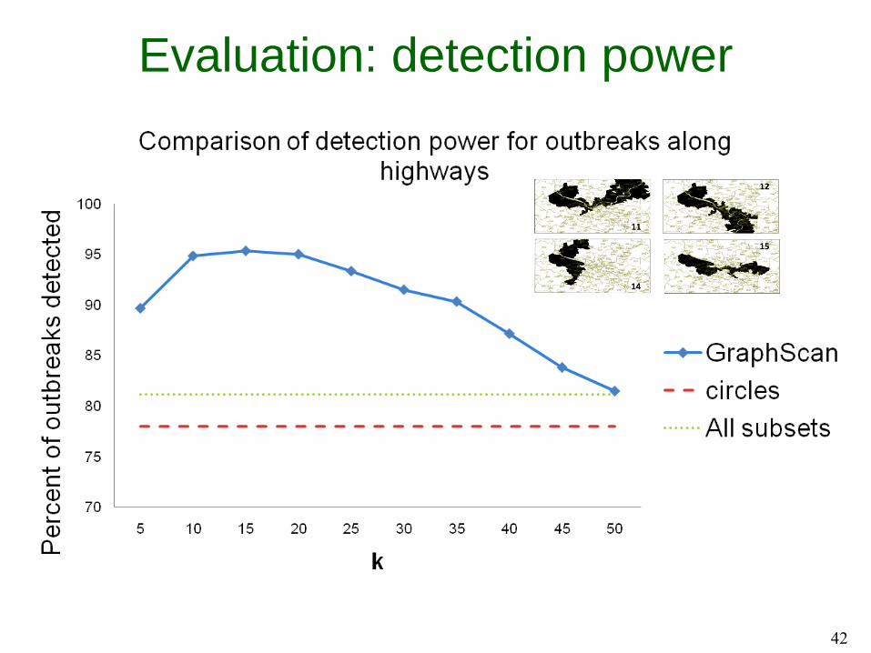
42
Evaluation: detection power

Extensions of GraphScan
What if we want to allow for
events which spread
dynamically over the
(static) graph structure?
Based on a new variant of the
LTSS property1, we can search
for dynamic patterns while
enforcing soft constraints on
temporal consistency.
We have applied this method for
accurate detection, tracking, and
source-tracing of contaminants
spreading through a water
distribution network.2
What if the underlying graph
structure is unknown?
We can accurately learn the
graph structure from unlabeled
outbreak data, and use the
learned structure for detection.
Often, the learned graph
enables even faster detection
of events than the true graph!3
1Speakman, Somanchi, McFowland, and
Neill. Penalized fast subset scanning. J
Comput Graph Stat 25(2): 382-404, 2016.
3Somanchi and Neill, submitted.
2Speakman, Zhang, Neill. Dynamic pattern
detection with temporal consistency and
connectivity constraints. Proc. ICDM 2013.
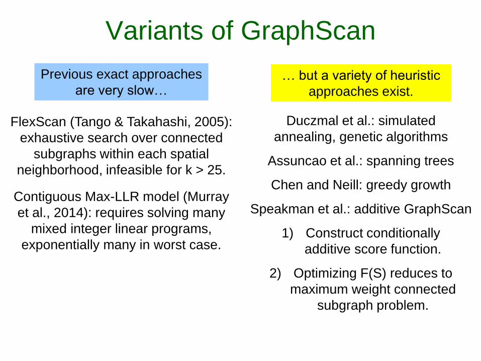
Variants of GraphScan
Previous exact approaches
are very slow…
FlexScan (Tango & Takahashi, 2005):
exhaustive search over connected
subgraphs within each spatial
neighborhood, infeasible for k > 25.
… but a variety of heuristic
approaches exist.
Duczmal et al.: simulated
annealing, genetic algorithms
Assuncao et al.: spanning trees
Chen and Neill: greedy growth
Speakman et al.: additive GraphScan
1) Construct conditionally
additive score function.
2) Optimizing F(S) reduces to
maximum weight connected
subgraph problem.
Contiguous Max-LLR model (Murray
et al., 2014): requires solving many
mixed integer linear programs,
exponentially many in worst case.

Taxonomy
45
Anomalous & significant subgraph detection
Static attributed networks Dynamic attributed networks
Fast subset
scan
Complex networksSpatial networks
Graph
scan
Nonparametric
graph scan
Submodular
optimization
methods
Graph-structured
Sparse optimization
methods

Event Detection from Social Media
Protest in Mexico, 7/14/2012 2012 Washington D.C. Traffic Tweet Map for 2011 VA Earthquake
(Chen and Neill, KDD 2014)
Social media is a real-time “sensor” of large-scale population
behavior, and can be used for early detection of emerging events...
… but it is very complex, noisy, and subject to biases.
We have developed a new event detection methodology:
“Non-Parametric Heterogeneous Graph Scan” (NPHGS)
Applied to: civil unrest prediction, rare disease outbreak detection,
and early detection of human rights events.

Technical Challenges
Integration of multiple
heterogeneous
information sources!

Technical Challenges
Hashtag “#Megamarch”
mentioned 1,000 times
Influential user “Zeka”
posted 10 tweets
Mexico City has
5,000 active users
and 100,000 tweets
Tweets that have been
re-tweeted 1,000 times
A specific link (URL)
was mentioned
866 times
Keyword “Protest”
mentioned 5,000 times
One week before Mexico’s 2012 presidential election:

Twitter Heterogeneous Network
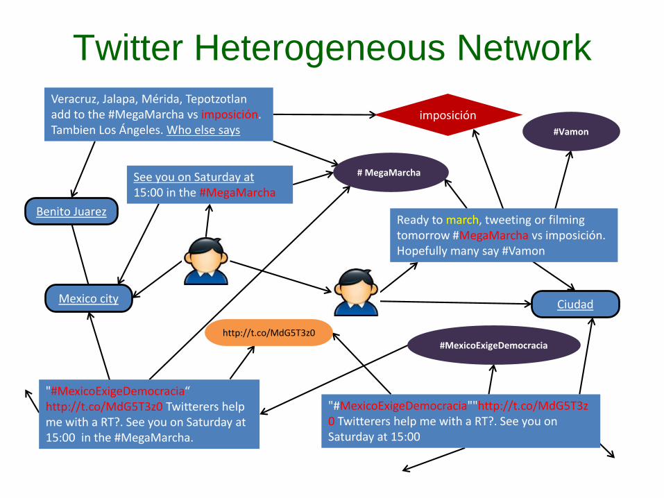
"#MexicoExigeDemocracia“ http://t.co/MdG5T3z0 Twitterers help me with a RT?. See you on Saturday at 15:00 in the #MegaMarcha.
"#MexicoExigeDemocracia""http://t.co/MdG5T3z0 Twitterers help me with a RT?. See you on Saturday at 15:00
Ready to march, tweeting or filming tomorrow #MegaMarcha vs imposición. Hopefully many say #Vamon
#MexicoExigeDemocraciahttp://t.co/MdG5T3z0
Veracruz, Jalapa, Mérida, Tepotzotlanadd to the #MegaMarcha vs imposición. Tambien Los Ángeles. Who else says
imposición
# MegaMarchaSee you on Saturday at15:00 in the #MegaMarcha
Mexico city
Benito Juarez
Ciudad
#Vamon
Twitter Heterogeneous Network
Twitter Heterogeneous Network

Nonparametric Heterogeneous Graph Scan
1) We model the heterogeneous social network as a sensor network.
Each node senses its local neighborhood, computes multiple
features, and reports the overall degree of anomalousness.
2) We compute an empirical p-value for each node:
• Uniform on [0,1] under the null hypothesis of no events.
• We search for subgraphs of the network with a higher than
expected number of low (significant) empirical p-values.
3) We can scale up to very large heterogeneous networks:
• Heuristic approach: iterative subgraph expansion (“greedy
growth” to subset of neighbors on each iteration).
• We can efficiently find the best subset of neighbors, ensuring
that the subset remains connected, at each step.
(Chen and Neill, KDD 2014)

empirical
calibration
empirical
calibration
Sensor network modeling
Object Type Features
User # tweets, # retweets, # followers, #followees,
#mentioned_by, #replied_by,
diffusion graph depth, diffusion graph size
Tweet Klout, sentiment, replied_by_graph_size, reply_graph_size,
retweet_graph_size, retweet_graph_depth
City, State, Country # tweets, # active users
Term # tweets
Link # tweets
Hashtag # tweets
Each node reports an empirical p-value measuring the current
level of anomalousness for each time interval (hour or day).
Individual p-value
for each featureFeatures
Minimum
empirical p-
value for
each node
Overall p-value
for each node
min
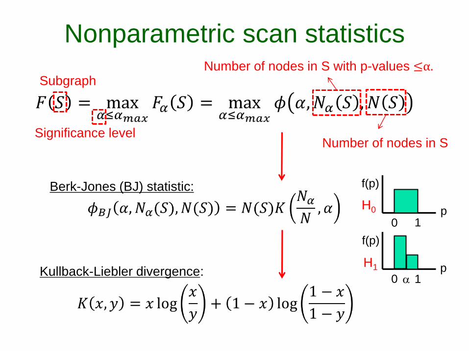
Nonparametric scan statistics
Subgraph
Berk-Jones (BJ) statistic:
Kullback-Liebler divergence:
Significance levelNumber of nodes in S
Number of nodes in S with p-values ≤α.
p
p
f(p)
f(p)
0
0
1
1
a
H0
H1
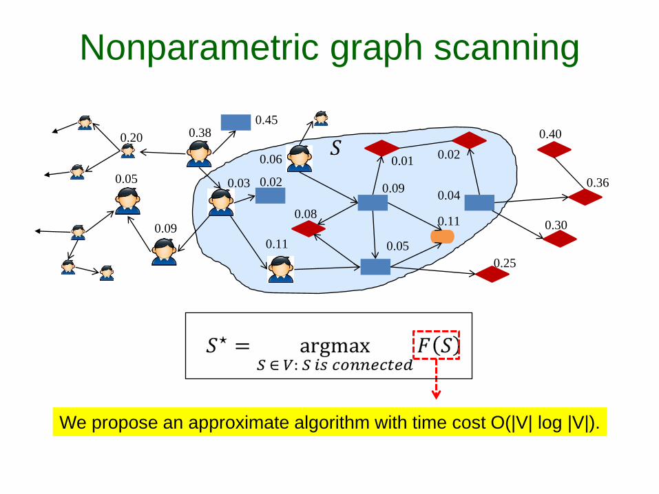
Nonparametric graph scanning
0.09
0.05
0.20
0.03
0.11
0.02
0.08
0.06
0.09
0.010.02
0.04
0.11
0.05
0.25
0.30
0.40
0.36
0.380.45
We propose an approximate algorithm with time cost O(|V| log |V|).

NPHGS evaluation- civil unrestCountry # of tweets News source*
Argentina 29,000,000 Clarín; La Nación; Infobae
Chile 14,000,000 La Tercera; Las Últimas Notícias; El Mercurio
Colombia 22,000,000 El Espectador; El Tiempo; El Colombiano
Ecuador 6,900,000 El Universo; El Comercio; Hoy
Gold standard dataset: 918 civil unrest events between July and December 2012.
We compared the detection performance of our NPHGS approach
to homogeneous graph scan methods and to a variety of state-of-
the-art methods previously proposed for Twitter event detection.
Example of a gold standard event label:
PROVINCE = “El Loa” COUNTRY = “Chile”
DATE = “2012-05-18” LINK = “http://www.pressenza.com/2012/05/...”
DESCRIPTION = “A large-scale march was staged by inhabitants of the
northern city of Calama, considered the mining capital of Chile, who
demanded the allocation of more resources to copper mining cities”

NPHGS results- civil unrest
NPHGS outperforms existing representative techniques for both event
detection and forecasting, increasing detection power, forecasting
accuracy, and forecasting lead time while reducing time to detection.
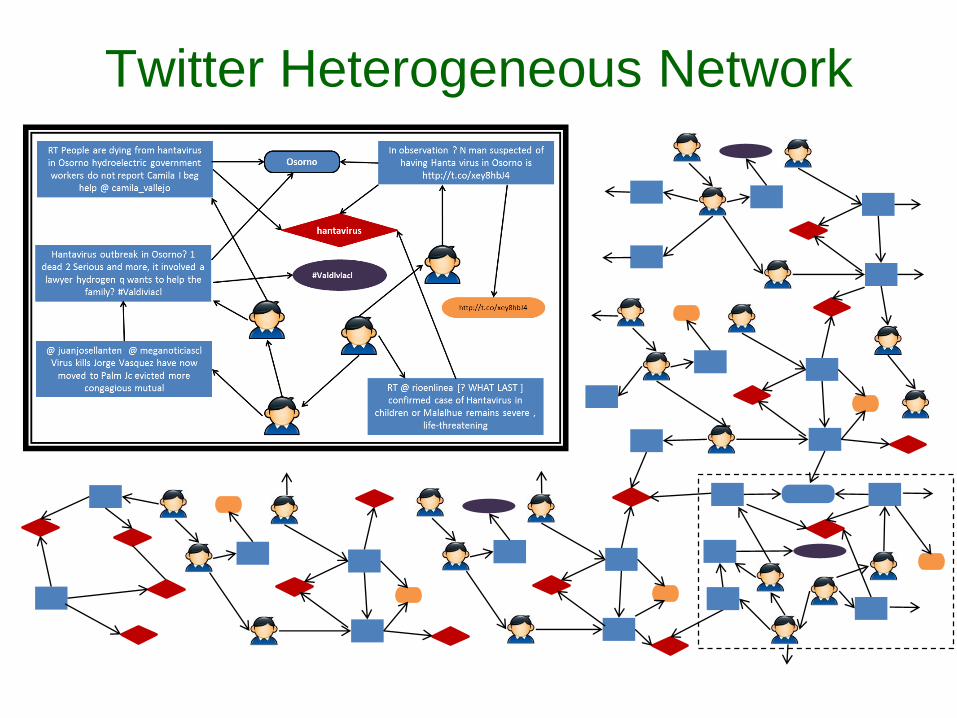
Similar improvements in performance were observed on a second task:
Early detection of rare disease outbreaks, using gold standard data
about 17 hantavirus outbreaks from the Chilean Ministry of Health.

Taxonomy
60
Anomalous & significant subgraph detection
Static attributed networks Dynamic attributed networks
Fast subset
scan
Complex networksSpatial networks
Graph
scan
Nonparametric
graph scan
Submodular
optimization
methods
Graph-structured
Sparse optimization
methods

Subgraph detection via submodular
optimization• A class of subgraph detection problems can
be framed as a general submodular (but not
monotone) maximization problem:
61
maxS F(S)+l ×D(S)
A submodular score function that
characterizes the level of
anomalousness of the subset of
nodes S.
A submodular compactness
function that gives a higher
score if the subset of nodes S is
more compact.
(Rozenshtein et al.,
KDD 2014)

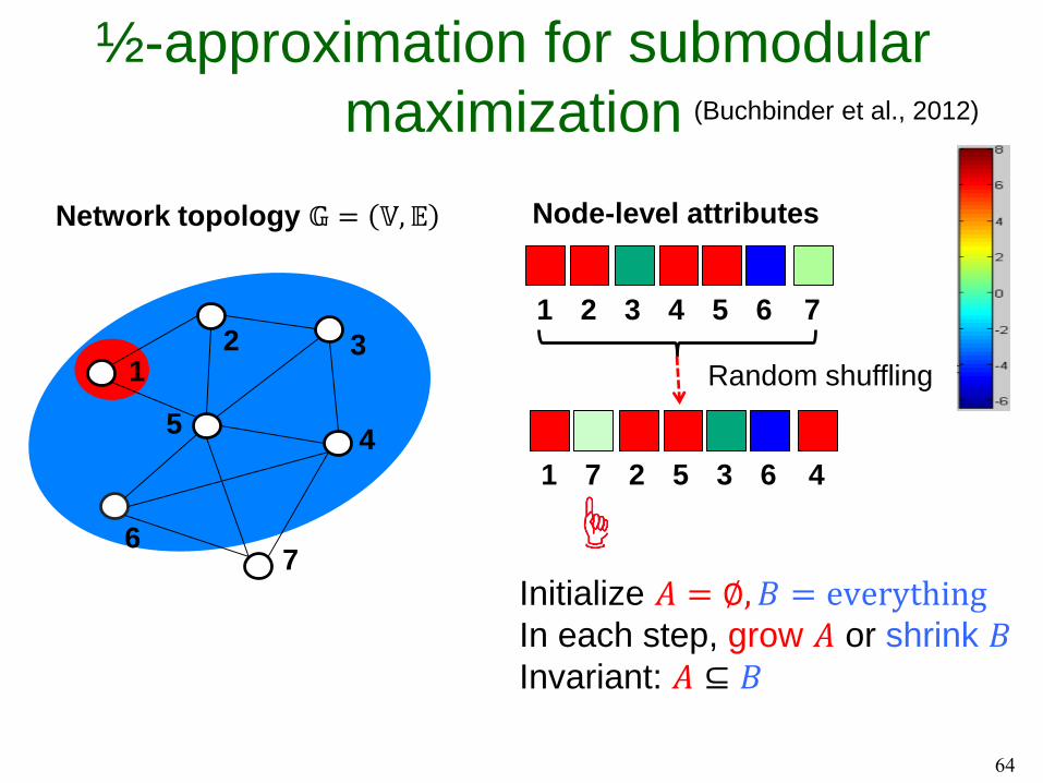
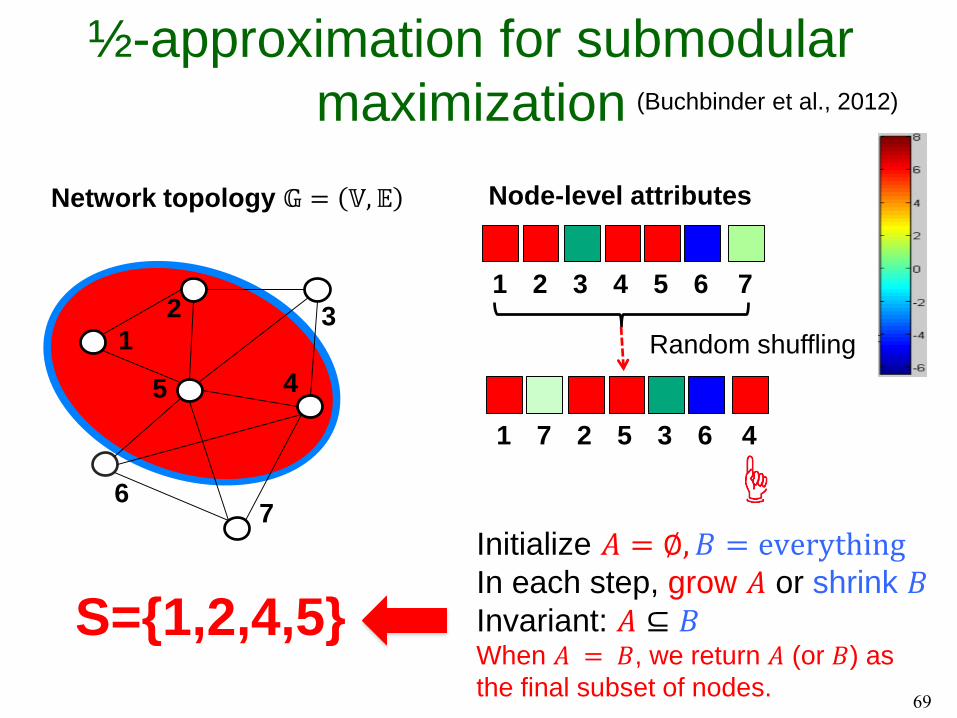
½-approximation for submodular
maximization
62
12 3
45
67
1
Network topology 𝔾 = 𝕍, 𝔼
Initialize 𝐴 = ∅, 𝐵 = everythingIn each step, grow 𝐴 or shrink 𝐵Invariant: 𝐴 ⊆ 𝐵
Node-level attributes
Random shuffling
2 3 4 5 6 7
1 7 2 5 3 6 4
(Buchbinder et al., 2012)
∅

½-approximation for submodular
maximization
63
12 3
45
67
1
Network topology 𝔾 = 𝕍, 𝔼
Initialize 𝐴 = ∅, 𝐵 = everythingIn each step, grow 𝐴 or shrink 𝐵Invariant: 𝐴 ⊆ 𝐵
Node-level attributes
Random shuffling
2 3 4 5 6 7
1 7 2 5 3 6 4
(Buchbinder et al., 2012)
½-approximation for submodular
maximization
64
12 3
45
67
1
Network topology 𝔾 = 𝕍, 𝔼 Node-level attributes
Random shuffling
2 3 4 5 6 7
1 7 2 5 3 6 4
Initialize 𝐴 = ∅, 𝐵 = everythingIn each step, grow 𝐴 or shrink 𝐵Invariant: 𝐴 ⊆ 𝐵
(Buchbinder et al., 2012)

½-approximation for submodular
maximization
65
1
2 3
45
67
1
Network topology 𝔾 = 𝕍, 𝔼 Node-level attributes
Random shuffling
2 3 4 5 6 7
1 7 2 5 3 6 4
Initialize 𝐴 = ∅, 𝐵 = everythingIn each step, grow 𝐴 or shrink 𝐵Invariant: 𝐴 ⊆ 𝐵
(Buchbinder et al., 2012)

½-approximation for submodular
maximization
66
1
2 3
45
67
1
Network topology 𝔾 = 𝕍, 𝔼 Node-level attributes
Random shuffling
2 3 4 5 6 7
1 7 2 5 3 6 4
Initialize 𝐴 = ∅, 𝐵 = everythingIn each step, grow 𝐴 or shrink 𝐵Invariant: 𝐴 ⊆ 𝐵
(Buchbinder et al., 2012)

½-approximation for submodular
maximization
67
1
2 3
45
67
1
Network topology 𝔾 = 𝕍, 𝔼 Node-level attributes
Random shuffling
2 3 4 5 6 7
1 7 2 5 3 6 4
Initialize 𝐴 = ∅, 𝐵 = everythingIn each step, grow 𝐴 or shrink 𝐵Invariant: 𝐴 ⊆ 𝐵
(Buchbinder et al., 2012)

½-approximation for submodular
maximization
68
1
2 3
45
67
1
Network topology 𝔾 = 𝕍, 𝔼 Node-level attributes
Random shuffling
2 3 4 5 6 7
1 7 2 5 3 6 4
Initialize 𝐴 = ∅, 𝐵 = everythingIn each step, grow 𝐴 or shrink 𝐵Invariant: 𝐴 ⊆ 𝐵
(Buchbinder et al., 2012)
½-approximation for submodular
maximization
69
1
2 3
45
67
1
Network topology 𝔾 = 𝕍, 𝔼 Node-level attributes
Random shuffling
2 3 4 5 6 7
1 7 2 5 3 6 4
S={1,2,4,5}
Initialize 𝐴 = ∅, 𝐵 = everythingIn each step, grow 𝐴 or shrink 𝐵Invariant: 𝐴 ⊆ 𝐵When 𝐴 = 𝐵, we return 𝐴 (or 𝐵) as
the final subset of nodes.
(Buchbinder et al., 2012)

Case studies: event detection
• Bicing sensor networks
70
(Rozenshtein et al.,
KDD 2014)
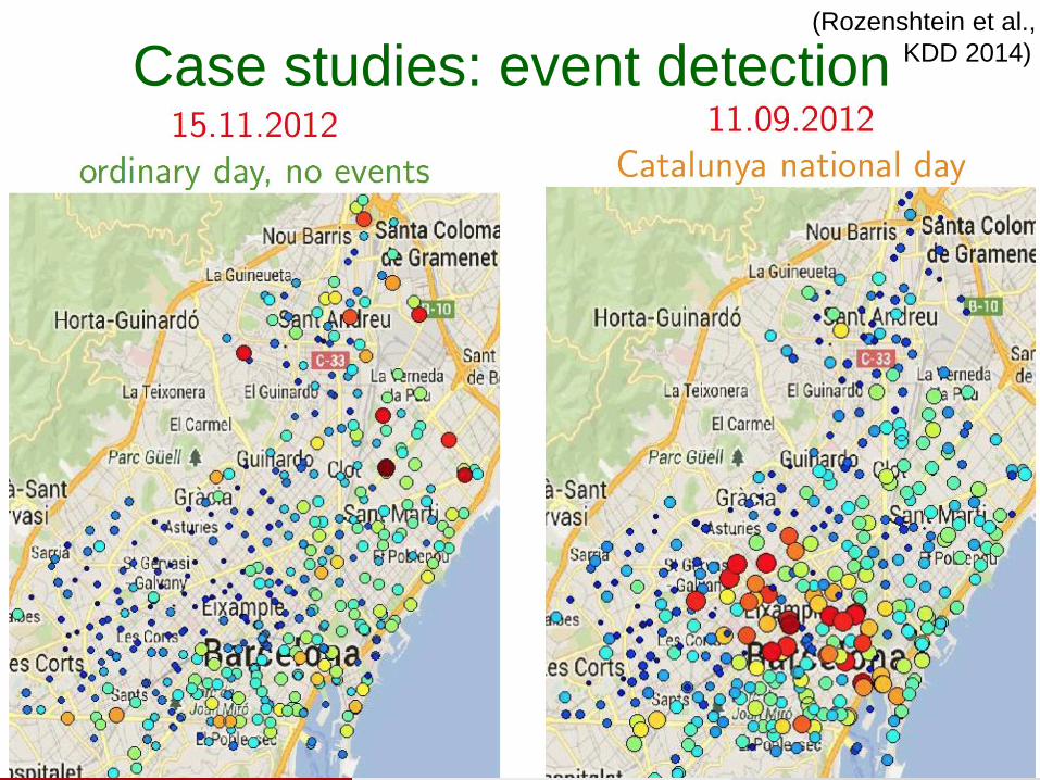
Case studies: event detection
• Sensor networks and traffic networks
71
(Rozenshtein et al.,
KDD 2014)

Case studies: event detection
• Events discovered with bicing data
72
(Rozenshtein et al.,
KDD 2014)

Taxonomy
73
Anomalous & significant subgraph detection
Static attributed networks Dynamic attributed networks
Fast subset
scan
Complex networksSpatial networks
Graph
scan
Nonparametric
graph scan
Submodular
optimization
methods
Graph-structured
Sparse optimization
methods

Graph structured sparse optimization
The problem of subgraph detection
can be reformulated as
where supp 𝒚 = 𝑖 | 𝑦𝑖 > 0 and 𝑆 can be identified as
𝑆 = supp 𝒚 , and 𝑓 𝒚 = 𝐹(𝑆)
74
max𝑆⊆𝑉
𝐹(𝑆) 𝑠. 𝑡. 𝑆 satisfies a predefinedtopological constraint.
max𝒚⊆ 0,1 𝑛
𝑓(𝒚) 𝑠. 𝑡. supp(𝒚) satisfies a predefinedtopological constraint.

Graph structured sparse optimization
• This approach solves the relaxed problem
• Three novel sparse optimization algorithms
• Graph-structured iterative hard thresholding
(Graph-IHT).
• Graph-structured gradient hard thresholding
Pursuit (Graph-GHTP).
• Graph-structured matching pursuit (Graph-MP)
75
max𝒚⊆ 0,1 𝑛
𝑓(𝒚) 𝑠. 𝑡. supp(𝒚) satisfies a predefinedtopological constraint.
(Zhou and Chen, ICDM, 2016)
(Zhou and Chen, ICDM, 2016)
(Chen and Zhou, IJCAI, 2016)

Interpretation of projection oracle
• A projection oracle P(𝒃) is defined as
76
P 𝒃 = arg min𝒚∈ℝ𝑛
𝒚 − 𝒃 22 s.t. supp 𝒚 is a connected
subset of size at most 4.
𝒃
Feasible set of
connected subsets
of size at most 4.
P 𝒃
Contour of 𝑓 𝒚
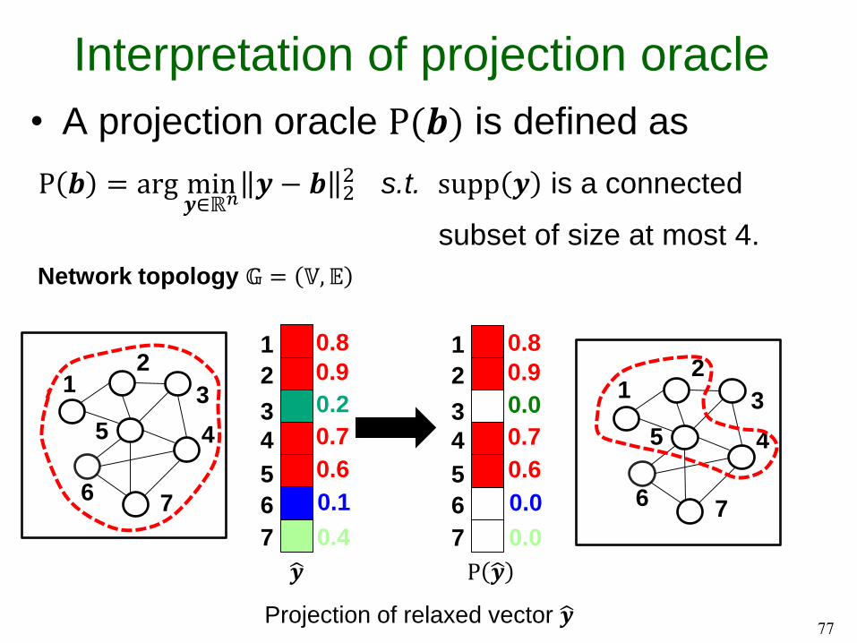
Interpretation of projection oracle
• A projection oracle P(𝒃) is defined as
77
12
3
45
6 7
1
Network topology 𝔾 = 𝕍, 𝔼
2
3
4
5
6
7
0.8
0.9
0.2
0.7
0.6
0.1
0.4
1
2
3
4
5
6
7
12
3
45
6 7
0.8
0.9
0.0
0.7
0.6
0.0
0.0
Projection of relaxed vector 𝒚
𝒚 P 𝒚
P 𝒃 = arg min𝒚∈ℝ𝑛
𝒚 − 𝒃 22 s.t. supp 𝒚 is a connected
subset of size at most 4.

Interpretation of projection oracle
• A projection oracle P(𝒃) is defined as
78
12
3
45
6 7
1
Network topology 𝔾 = 𝕍, 𝔼
2
3
4
5
6
7
P 𝒃 = arg min𝒚∈ℝ𝑛
𝒚 − 𝒃 22 s.t. supp 𝒚 is a connected
subset of size at most 4.
+2
+3
-1
+4
+2
-4
-1
1
2
3
4
5
6
7
+0
+3
-0
+4
+2
-4
-0
12
3
45
6 7
Projection of a gradient 𝛻𝑓 𝒚 .
𝛻𝑓 𝒚 P 𝛻𝑓 𝒚

Description of the Graph-IHT algorithm
79
Projection on the
gradient 𝛻𝑓 𝒚𝑖
Projection on an
intermediate solution 𝒃
(Zhou and Chen, ICDM, 2016)
+
supp

ℳ 𝔾,𝑘 = 5 = 𝒚 | 𝒚 ∈ 0,1 𝑛, supp 𝒚 ∈ 𝕄 𝔾, 𝑘 = 5Network instance 𝔾
𝑓 𝒚
Illustration of the Graph-IHT algorithm(Zhou and Chen, ICDM, 2016)
𝕄 𝔾, 𝑘 = 5 represents the space of
connected subsets of size at most 5.

ℳ 𝔾,𝑘 = 5 = 𝑦 | 𝑦 ∈ 0,1 𝑛, supp 𝑦 ∈ 𝕄 𝔾, 𝑘 = 5Network instance 𝔾
𝔾supp 𝒚⋆
𝑓 𝒚
Illustration of the Graph-IHT algorithm(Zhou and Chen, ICDM, 2016)

ℳ 𝔾,𝑘 = 5 = 𝒚 | 𝒚 ∈ 0,1 𝑛, supp 𝒚 ∈ 𝕄 𝔾, 𝑘 = 5
𝒚0
Network instance 𝔾
𝔾supp 𝒚𝑖
𝑓 𝒚
Illustration of the Graph-IHT algorithm(Zhou and Chen, ICDM, 2016)

ℳ 𝔾,𝑘 = 5 = 𝒚 | 𝒚 ∈ 0,1 𝑛, supp 𝒚 ∈ 𝕄 𝔾, 𝑘 = 5
𝒚0
𝔾supp 𝒚𝑖
𝔾supp 𝒚0
𝑓 𝒚
Network instance 𝔾
Illustration of the Graph-IHT algorithm(Zhou and Chen, ICDM, 2016)

ℳ 𝔾,𝑘 = 5 = 𝒚 | 𝒚 ∈ 0,1 𝑛, supp 𝒚 ∈ 𝕄 𝔾, 𝑘 = 5
𝑦0
𝔾supp 𝒚𝑖
𝔾supp 𝒚0
𝛻𝑓 𝒚0
𝑓 𝒚
Network instance 𝔾
Illustration of the Graph-IHT algorithm(Zhou and Chen, ICDM, 2016)

ℳ 𝔾,𝑘 = 5 = 𝒚 | 𝒚 ∈ 0,1 𝑛, supp 𝒚 ∈ 𝕄 𝔾, 𝑘 = 5
𝑦0
𝔾supp 𝒚𝑖
𝔾supp 𝒚0
𝛻𝑓 𝒚𝟎
𝑓 𝒚 P 𝛻𝑓 𝒚0
Network instance 𝔾
Illustration of the Graph-IHT algorithm(Zhou and Chen, ICDM, 2016)

ℳ 𝔾,𝑘 = 5 = 𝒚 | 𝒚 ∈ 0,1 𝑛, supp 𝒚 ∈ 𝕄 𝔾, 𝑘 = 5
𝑦0
𝔾supp 𝒚𝑖
𝔾supp 𝒚0
P 𝛻𝑓 𝒚0
𝛻𝑓 𝒚0
𝑓 𝒚
𝐛 = 𝐲0 + 𝜂 ⋅ P 𝛻𝑓 𝒚0
Network instance 𝔾
Illustration of the Graph-IHT algorithm(Zhou and Chen, ICDM, 2016)

ℳ 𝔾,𝑘 = 5 = 𝒚 | 𝒚 ∈ 0,1 𝑛, supp 𝒚 ∈ 𝕄 𝔾, 𝑘 = 5
𝑦0
𝔾supp 𝒚𝑖
𝔾supp 𝒚0
H 𝛻𝑓 𝑦0
𝛻𝑓 𝒚0
𝑓 𝒚
𝐛 = 𝐲0 + 𝜂 ⋅ H 𝛻𝑓 𝒚0
𝒚1 = T(𝒃)
Network instance 𝔾
Illustration of the Graph-IHT algorithm(Zhou and Chen, ICDM, 2016)

ℳ 𝔾,𝑘 = 5 = 𝒚 | 𝒚 ∈ 0,1 𝑛, supp 𝒚 ∈ 𝕄 𝔾, 𝑘 = 5
𝑦0
𝔾supp 𝒚𝑖
𝔾supp 𝒚0
H 𝛻𝑓 𝒚0
𝛻𝑓 𝒚0
𝑓 𝒚
𝐛 = 𝐲0 + 𝜂 ⋅ H 𝛻𝑓 𝒚0
𝒚1 = T(𝒃)
𝔾supp 𝒚1
Network instance 𝔾
Illustration of the Graph-IHT algorithm(Zhou and Chen, ICDM, 2016)

ℳ 𝔾,𝑘 = 5 = 𝒚 | 𝒚 ∈ 0,1 𝑛, supp 𝒚 ∈ 𝕄 𝔾, 𝑘 = 5
𝑦0
𝔾supp 𝒚𝑖
𝔾supp 𝒚0
H 𝛻𝑓 𝑦0
𝛻𝑓 𝒚0
𝑓 𝒚
𝐛 = 𝐲0 + 𝜂 ⋅ H 𝛻𝑓 𝒚0
𝒚1 = T(𝒃)
𝔾supp 𝒚1
Network instance 𝔾
Illustration of the Graph-IHT algorithm(Zhou and Chen, ICDM, 2016)

ℳ 𝔾,𝑘 = 5 = 𝒚 | 𝒚 ∈ 0,1 𝑛, supp 𝒚 ∈ 𝕄 𝔾, 𝑘 = 5
𝑦0
𝔾supp 𝒚𝑖
𝔾supp 𝒚0
H 𝛻𝑓 𝑦0
𝛻𝑓 𝒚0
𝑓 𝒚
𝐛 = 𝐲0 + 𝜂 ⋅ H 𝛻𝑓 𝒚0
𝒚1 = T(𝒃)
𝔾supp 𝒚1
Network instance 𝔾
Illustration of the Graph-IHT algorithm(Zhou and Chen, ICDM, 2016)

ℳ 𝔾,𝑘 = 5 = 𝒚 | 𝒚 ∈ 0,1 𝑛, supp 𝒚 ∈ 𝕄 𝔾, 𝑘 = 5
𝑦0
𝔾supp 𝒚𝑖
𝔾supp 𝒚0
H 𝛻𝑓 𝑦0
𝛻𝑓 𝒚0
𝑓 𝒚
𝐛 = 𝐲0 + 𝜂 ⋅ H 𝛻𝑓 𝒚0
𝒚1 = T(𝒃)
𝔾supp 𝒚1
Network instance 𝔾
Illustration of the Graph-IHT algorithm(Zhou and Chen, ICDM, 2016)

ℳ 𝔾,𝑘 = 5 = 𝒚 | 𝒚 ∈ 0,1 𝑛, supp 𝒚 ∈ 𝕄 𝔾, 𝑘 = 5
𝑦0
𝔾supp 𝒚𝑖
𝔾supp 𝒚0
H 𝛻𝑓 𝑦0
𝛻𝑓 𝒚0
𝑓 𝒚
𝐛 = 𝐲0 + 𝜂 ⋅ H 𝛻𝑓 𝒚0
𝒚1 = T(𝒃)
𝔾supp 𝒚1
Network instance 𝔾
Illustration of the Graph-IHT algorithm(Zhou and Chen, ICDM, 2016)

ℳ 𝔾,𝑘 = 5 = 𝒚 | 𝒚 ∈ 0,1 𝑛, supp 𝒚 ∈ 𝕄 𝔾, 𝑘 = 5
𝑦0
𝔾supp 𝒚𝑖
𝔾supp 𝒚0
H 𝛻𝑓 𝑦0
𝛻𝑓 𝒚0
𝑓 𝒚
𝐛 = 𝐲0 + 𝜂 ⋅ H 𝛻𝑓 𝒚0
𝒚1 = T(𝒃)
𝔾supp 𝒚1
Network instance 𝔾
Illustration of the Graph-IHT algorithm(Zhou and Chen, ICDM, 2016)
𝒚𝑖

Theoretical Guarantees
• The proposed algorithms have the following
nice theoretical properties
• Nearly-linear time complexity.
• Let 𝒚⋆ be the optimal solution of the relaxed
problem. Under practical assumptions, we have
the tight error bound
where
• 𝑐 is a constant value, and
• 𝐼 = argmaxS
𝛻𝑆𝑓 𝒚⋆ 2 s. t. 𝑆 satisfies the predefined
topological constraint.
𝒚⋆ − 𝒚𝑖2≤ 𝑐 ⋅ 𝛻𝐼𝑓 𝒚⋆ 2
(Zhou and Chen, ICDM, 2016)

Experiments
• Four real datasets for anomalous subgraph
detection
95
Comparison on
scores of the
identified subgraphs

Review of other methods
• Scalable anomaly ranking of attributed
neighborhoods• Rank a predefined set of neighborhoods (subgraphs)
based on internal connectivity, boundary, and node-level
attributes in quadratic time in the neighborhood size.
• Focused cluster or subgraph outlier
detection• Given an initial set of nodes provided by a user
• Step 1: Identify a subset of attributes that the given
nodes agree on (called “focus attributes”)
• Step 2: Find densely connected subgraphs that also
agree on these attributes (called “focused clusters”)
96
(Perozzi et al., KDD, 2016)
(Perozzi and Akoglu, SDM, 2016)
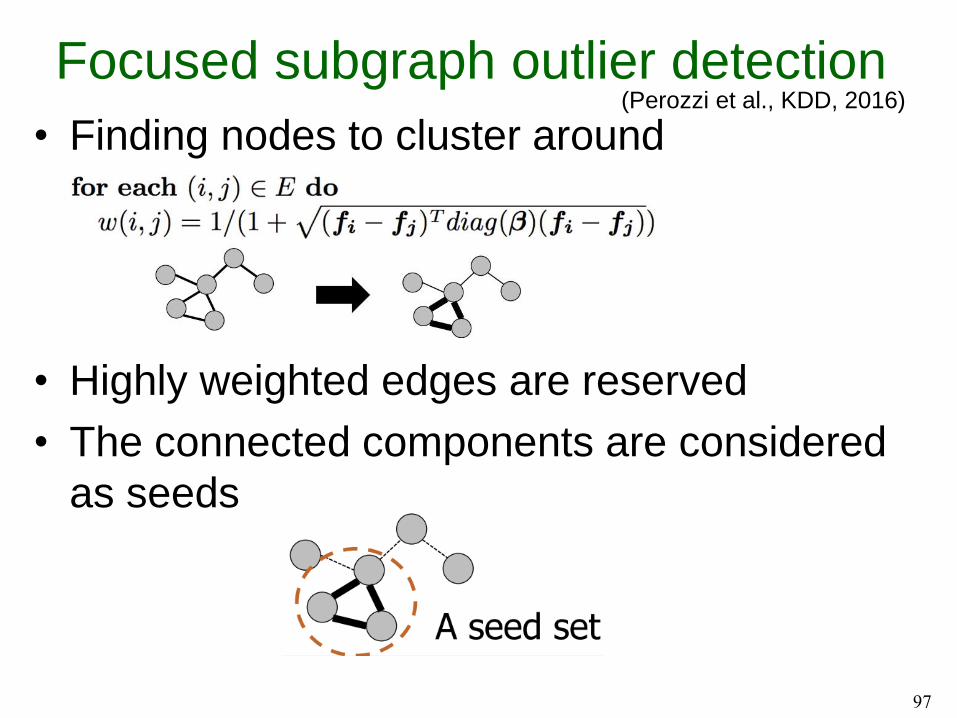
Focused subgraph outlier detection
• Finding nodes to cluster around
• Highly weighted edges are reserved
• The connected components are considered
as seeds
97
(Perozzi et al., KDD, 2016)

Focused subgraph outlier detection
1. Clustering objective: subgraph
conductance weighted by focus
2. At each edge in subgraph
expansion
1. Examine boundary nodes
2. Add node with the best marginal
gain
98
𝐹 𝑆 =WeightedOutDegree(S)
WeightedDensity S
(Perozzi et al., KDD, 2016)
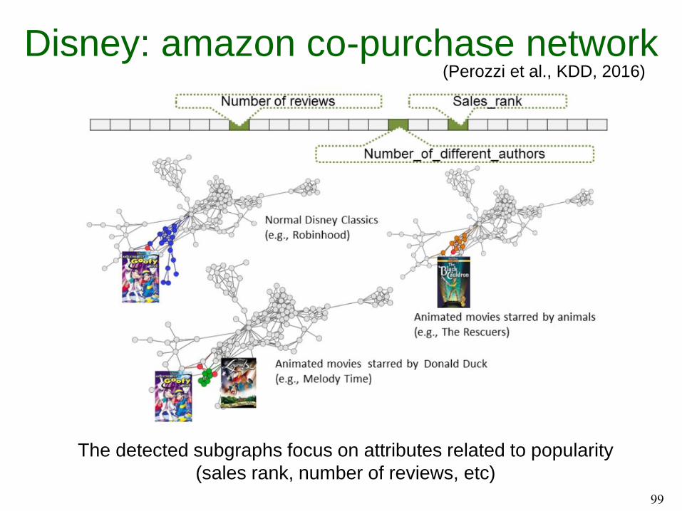
Disney: amazon co-purchase network
99
The detected subgraphs focus on attributes related to popularity
(sales rank, number of reviews, etc)
(Perozzi et al., KDD, 2016)

Political blogs citation network
100
A focused cluster of liberal blogs in Pol-Blogs with a focus on
Iraq ware debate
(Perozzi et al., KDD, 2016)

Part I: References• Kulldorff, M. (1997). A spatial scan statistic. Communications in Statistics-
Theory and methods, 26(6), 1481-1496.
• Neill, D. B., & Moore, A. W. (2005, August). Anomalous spatial cluster
detection. In Proceedings of the KDD 2005 Workshop on Data Mining
Methods for Anomaly Detection.
• Neill, D. B. (2012). Fast subset scan for spatial pattern detection. Journal
of the Royal Statistical Society: Series B (Statistical Methodology), 74(2),
337-360.
• Speakman, S., McFowland III, E., & Neill, D. B. (2015). Scalable detection
of anomalous patterns with connectivity constraints. Journal of
Computational and Graphical Statistics, 24(4), 1014-1033.
• Speakman, S., Somanchi, S., McFowland III, E., & Neill, D. B. (2016).
Penalized fast subset scanning. Journal of Computational and Graphical
Statistics, 25(2), 382-404.
• Speakman, S., Zhang, Y., & Neill, D. B. (2013, December). Dynamic
pattern detection with temporal consistency and connectivity constraints.
In 2013 IEEE 13th International Conference on Data Mining (pp. 697-706).
IEEE.101

Part I: References• Chen, F., & Neill, D. B. (2014, August). Non-parametric scan statistics for
event detection and forecasting in heterogeneous social media graphs.
In Proceedings of the 20th ACM SIGKDD international conference on
Knowledge discovery and data mining (pp. 1166-1175). ACM.
• Chen, F., & Neill, D. B. (2015). Human rights event detection from
heterogeneous social media graphs. Big Data, 3(1), 34-40.
• Rozenshtein, P., Anagnostopoulos, A., Gionis, A., & Tatti, N. (2014,
August). Event detection in activity networks. In Proceedings of the 20th
ACM SIGKDD international conference on Knowledge discovery and data
mining(pp. 1176-1185). ACM.
• Chen, F., & Zhou, B. (2016). A Generalized Matching Pursuit Approach for
Graph-Structured Sparsity. In Proc. IJCAI (pp. 1389-1395).
• Zhou, B., & Chen, F. (2016). Graph-Structured Sparse Optimization for
Connected Subgraph Detection. In Proc. ICDM (to appear).
• Buchbinder, N., Feldman, M., Naor, J. S., & Schwartz, R. (2012,
October). A Tight Linear Time (1/2)-Approximation for Unconstrained
Submodular Maximization. In Proc. FOCS (pp. 649-658).
102

Part I: References• Neill, D. B., McFowland, E., & Zheng, H. (2013). Fast subset scan for
multivariate event detection. Statistics in medicine, 32(13), 2185-2208.
• Neill, D. B., & Cooper, G. F. (2010). A multivariate Bayesian scan statistic
for early event detection and characterization. Machine learning, 79(3),
261-282.
• Perozzi, B., & Akoglu, L. (2015). Scalable anomaly ranking of attributed
neighborhoods. In Proc. SDM, 207-215.
• Perozzi, B., Akoglu, L., Iglesias Sánchez, P., & Müller, E. (2014).
Focused clustering and outlier detection in large attributed graphs. In Proc.
KDD, 1346-1355.
• Akoglu, L., Tong, H., & Koutra, D. (2015). Graph based anomaly detection
and description: a survey. Data Mining and Knowledge Discovery, 29(3),
626-688.
• Bindu, P. V., & Thilagam, P. S. (2016). Mining social networks for
anomalies: Methods and challenges. Journal of Network and Computer
Applications, 68, 213-229.
103

Part I: References• Kuo, T. W., Lin, K. C. J., & Tsai, M. J. (2015). Maximizing submodular set
function with connectivity constraint: Theory and application to
networks. IEEE/ACM Transactions on Networking (TON), 23(2), 533-546.
• Hegde, C., Indyk, P., & Schmidt, L. (2015). A nearly-linear time framework
for graph-structured sparsity. In Proceedings of the 32nd International
Conference on Machine Learning (ICML-15) (pp. 928-937).
• Chuang, H. Y., Lee, E., Liu, Y. T., Lee, D., & Ideker, T. (2007).
Network‐based classification of breast cancer metastasis. Molecular
systems biology, 3(1), 140.
• de Oliveira, D. P., Neill, D. B., Garrett Jr, J. H., & Soibelman, L. (2010).
Detection of patterns in water distribution pipe breakage using spatial scan
statistics for point events in a physical network. Journal of Computing in
Civil Engineering, 25(1), 21-30.
104

5 minutes break: Q/A
105