announcements - university of california, irvinejutts/8/lecture20.pdfannouncements: •discussion...

Announcements:•Discussion today is review for midterm, no credit. You may attend more than one discussion section. •Bring 2 sheets of notes and calculator to midterm. We will provide Scantron form.

Homework: (Due Wed)Chapter 10: #5, 22, 42

Copyright ©2004 Brooks/Cole, a division of Thomson Learning, Inc., updated by Jessica Utts Feb 2010

Estimating Proportions

with Confidence

Chapter 10

Reminder from when we started Chapter 9 Five situations we will cover for the rest of this quarter:

Parameter name and description Population parameter Sample statistic For Categorical Variables: One population proportion (or probability) p p̂ Difference in two population proportions p1 – p2 21 ˆˆ pp − For Quantitative Variables: One population mean µ x Population mean of paired differences (dependent samples, paired) µd d Difference in two population means (independent samples) µ1 − µ2 21 xx −

For each situation will we: √ Learn about the sampling distribution for the sample statistic • Learn how to find a confidence interval for the true value of the

parameter • Test hypotheses about the true value of the parameter


3

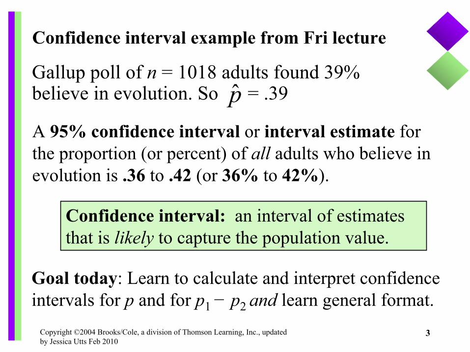
Confidence interval example from Fri lecture

Gallup poll of n = 1018 adults found 39% believe in evolution. So = .39

A 95% confidence interval or interval estimate for the proportion (or percent) of all adults who believe in evolution is .36 to .42 (or 36% to 42%).

Confidence interval: an interval of estimates that is likely to capture the population value.

Goal today: Learn to calculate and interpret confidence intervals for p and for p1− p2 and learn general format.

p̂


4

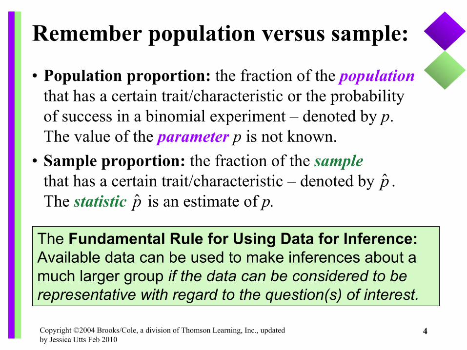
Remember population versus sample:

• Population proportion: the fraction of the populationthat has a certain trait/characteristic or the probability of success in a binomial experiment – denoted by p. The value of the parameter p is not known.

• Sample proportion: the fraction of the samplethat has a certain trait/characteristic – denoted by . The statistic is an estimate of p.

The Fundamental Rule for Using Data for Inference: Available data can be used to make inferences about a much larger group if the data can be considered to be representative with regard to the question(s) of interest.

p̂p̂


5

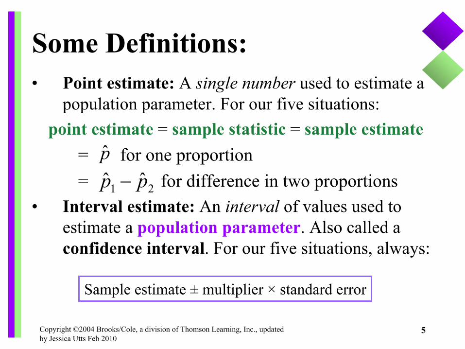
Some Definitions:• Point estimate: A single number used to estimate a

population parameter. For our five situations:point estimate = sample statistic = sample estimate

= for one proportion= for difference in two proportions

• Interval estimate: An interval of values used to estimate a population parameter. Also called a confidence interval. For our five situations, always:

p̂

21 ˆˆ pp −

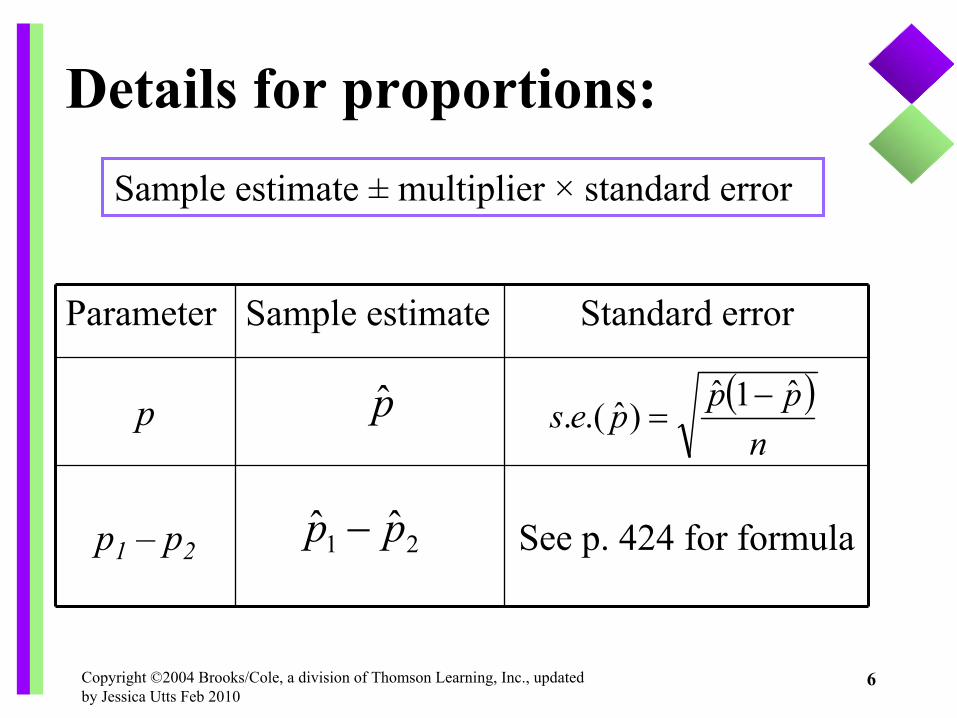
Sample estimate ± multiplier × standard error


6

Details for proportions:Sample estimate ± multiplier × standard error

Parameter Sample estimate Standard error

p

p1 – p2 See p. 424 for formula

p̂

21 ˆˆ pp −

( )n

pppesˆ1ˆ

)ˆ.(. −=


7

Multiplier and Confidence Level

• The multiplier is determined by the desired confidence level.

• The confidence level is the probability that the procedure used to determine the interval will provide an interval that includes the population parameter. Most common is .95.

• If we consider all possible randomly selected samples of same size from a population, the confidence level is the fraction or percent of those samples for which the confidence interval includes the population parameter.See picture on board.

• Often express the confidence level as a percent. Common levels are 90%, 95%, 98%, and 99%.


8

Note: Increase confidence level => larger multiplier.

More about the Multiplier

Multiplier, denoted as z*, is the standardized score such that the area between −z* and z* under the standard normal curve corresponds to the desired confidence level.


9

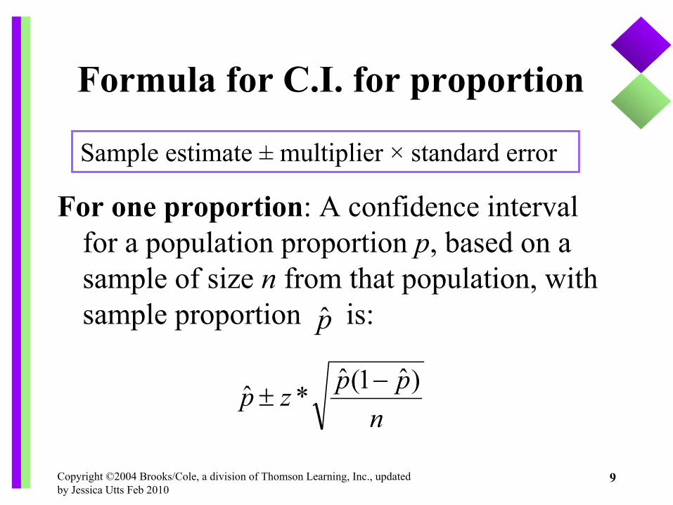
Formula for C.I. for proportion

For one proportion: A confidence interval for a population proportion p, based on a sample of size n from that population, with sample proportion is:


nppzp )ˆ1(ˆ

*ˆ −±

p̂


10

Example of different confidence levels

Poll on belief in evolution:n = 1018Sample proportion = .39Standard error =

90% confidence interval.39 ± 1.65(.0153) or .39 ± .025 or .365 to .41595% confidence interval:.39 ± 2(.0153) or .39 ± .03 or .36 to .4299% confidence interval.39 ± 2.58(.0153) or .39 ± .04 or .35 to .43

0153.1018

)39.1(39.)ˆ1(ˆ=

−=

−n

pp


11

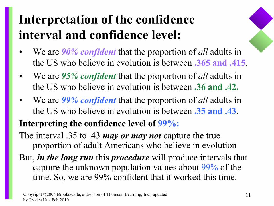
Interpretation of the confidence interval and confidence level:• We are 90% confident that the proportion of all adults in

the US who believe in evolution is between .365 and .415.• We are 95% confident that the proportion of all adults in

the US who believe in evolution is between .36 and .42.• We are 99% confident that the proportion of all adults in

the US who believe in evolution is between .35 and .43.Interpreting the confidence level of 99%:The interval .35 to .43 may or may not capture the true

proportion of adult Americans who believe in evolutionBut, in the long run this procedure will produce intervals that

capture the unknown population values about 99% of the time. So, we are 99% confident that it worked this time.


12

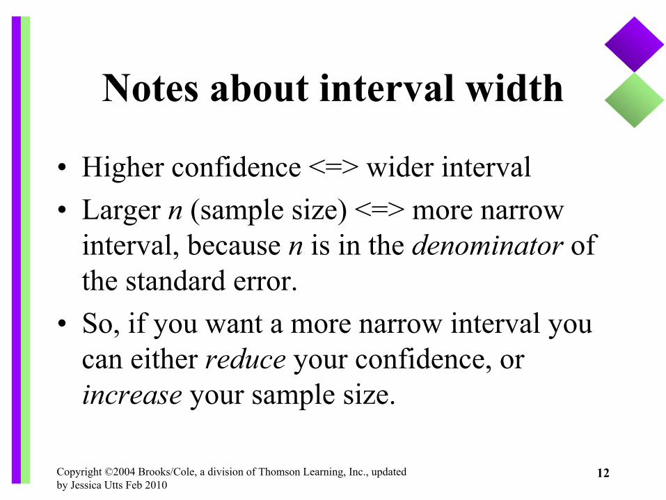
Notes about interval width

• Higher confidence <=> wider interval• Larger n (sample size) <=> more narrow

interval, because n is in the denominator of the standard error.

• So, if you want a more narrow interval you can either reduce your confidence, or increase your sample size.


13

Reconciling with Chapter 3formula for 95% confidence interval

Sample estimate ± Margin of errorwhere (conservative) margin of error was

n1

Now, “margin of error” is n

pp )ˆ1(ˆ2 −

These are the same when . The new margin of error is smaller for any other value of So we say the old version is conservative. It will give a wider interval.

5.ˆ =pp̂


14

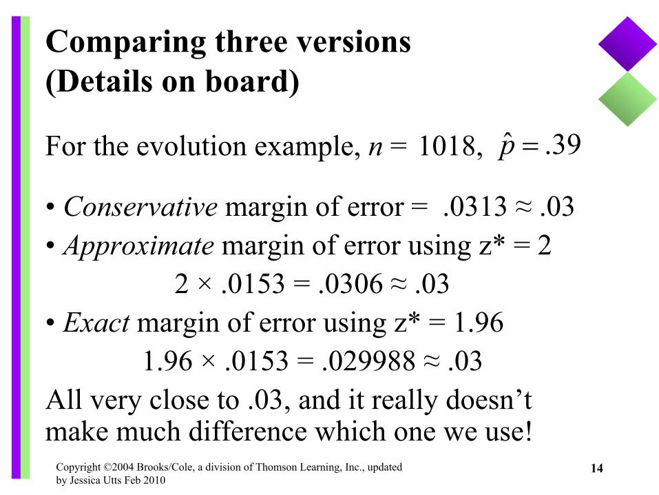
Comparing three versions(Details on board)

For the evolution example, n = 1018,

• Conservative margin of error = .0313 ≈ .03• Approximate margin of error using z* = 2

2 × .0153 = .0306 ≈ .03• Exact margin of error using z* = 1.96

1.96 × .0153 = .029988 ≈ .03All very close to .03, and it really doesn’t make much difference which one we use!

39.ˆ =p


15

New example: compare methods

Marist Poll in Oct 2009 asked “How often do you text while driving?” n = 1026

Nine percent answered “Often” or “sometimes” so and

• Conservative margin of error = .0312• Approximate margin of error = 2 × .009 = .018.This time, they are quite different! The conservative one is too conservative, it’s double

the approximate one!

009.1026

)91(.09.)ˆ.(. ==pes09.ˆ =p


16

Comparing margin of error• Conservative margin of error will be okay for

sample proportions near .5.• For sample proportions far from .5, closer to

0 or 1, don’t use the conservative margin of error. Resulting interval is wider than needed.

• Note that using a multiplier of 2 is called the approximate margin of error; the exact one uses multiplier of 1.96. It will rarely matter if we use 2 instead of 1.96.


17

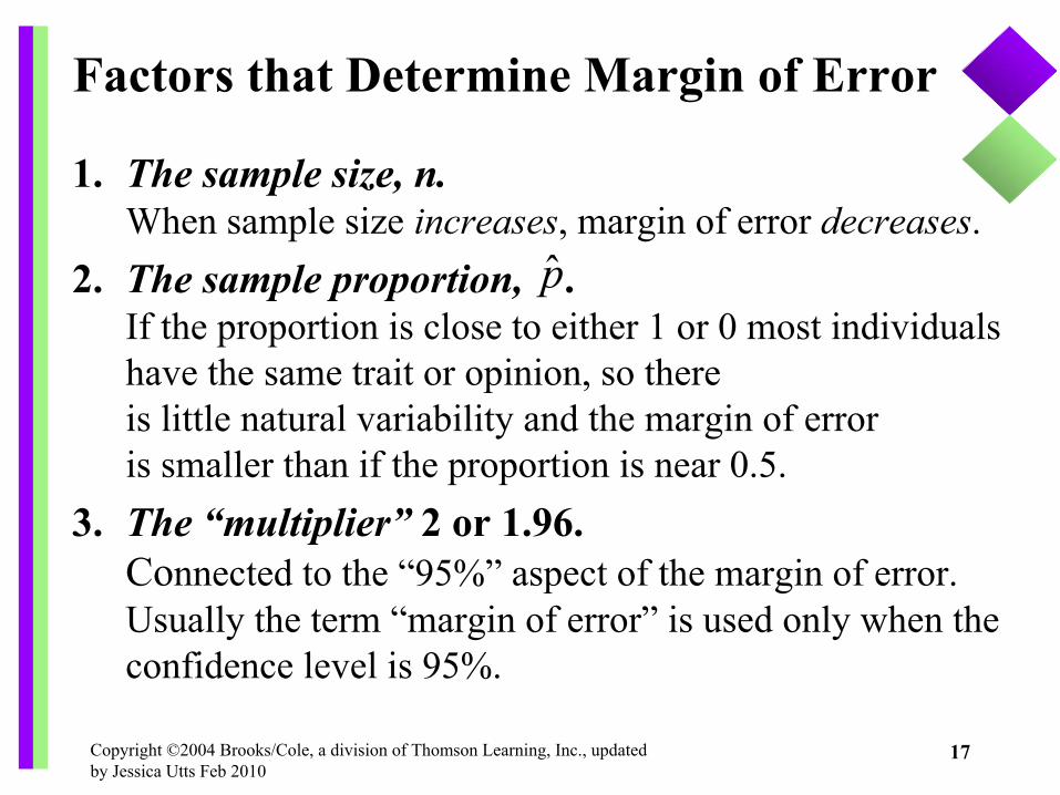
Factors that Determine Margin of Error

1. The sample size, n. When sample size increases, margin of error decreases.

2. The sample proportion, . If the proportion is close to either 1 or 0 most individuals have the same trait or opinion, so there is little natural variability and the margin of error is smaller than if the proportion is near 0.5.

3. The “multiplier” 2 or 1.96. Connected to the “95%” aspect of the margin of error. Usually the term “margin of error” is used only when the confidence level is 95%.

p̂


18

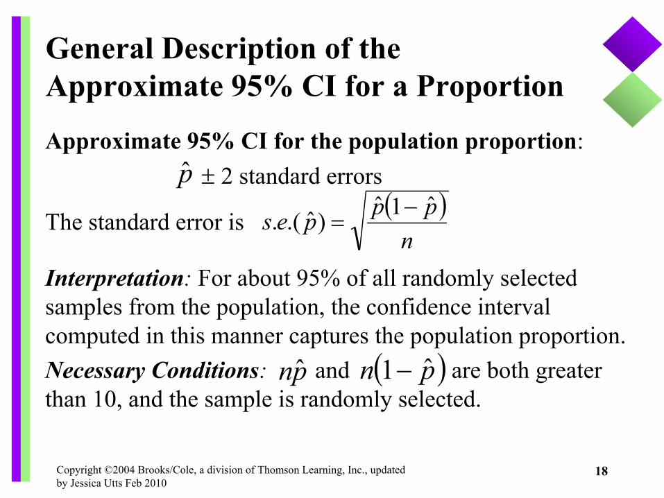
Approximate 95% CI for the population proportion:± 2 standard errors

The standard error is

Interpretation: For about 95% of all randomly selected samples from the population, the confidence interval computed in this manner captures the population proportion.Necessary Conditions: and are both greater than 10, and the sample is randomly selected.

General Description of the Approximate 95% CI for a Proportion

p̂( )

npppesˆ1ˆ

)ˆ.(. −=

pnˆ ( )pn ˆ1−


19

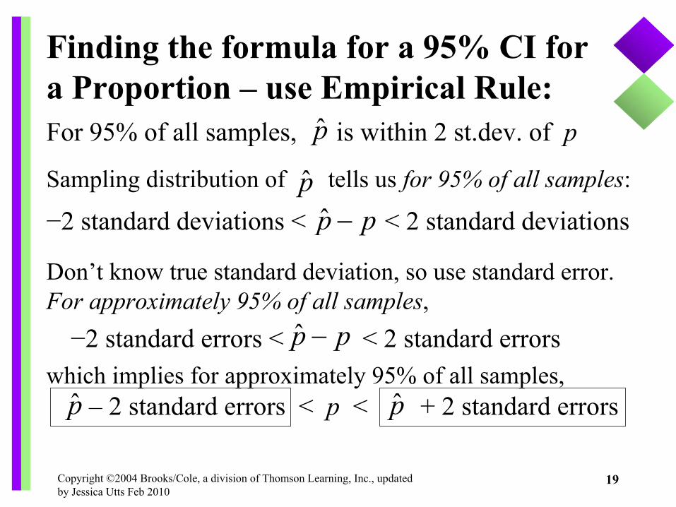
Sampling distribution of tells us for 95% of all samples:

−2 standard deviations < < 2 standard deviations

Don’t know true standard deviation, so use standard error.For approximately 95% of all samples, −2 standard errors < < 2 standard errors

which implies for approximately 95% of all samples, – 2 standard errors < p < + 2 standard errors

Finding the formula for a 95% CI for a Proportion – use Empirical Rule:For 95% of all samples, is within 2 st.dev. of p

p̂ p−p̂

p̂p̂

p̂

p̂ p−


20

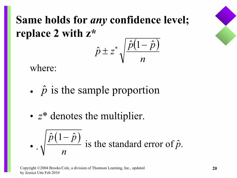
where:

•

• z* denotes the multiplier.

• .

Same holds for any confidence level; replace 2 with z*

( )ˆ ˆ1ˆis the standard error of .

p pp

n−

( )n

ppzpˆ1ˆˆ −

± ∗

ˆ is the sample proportionp


21

Example 10.3 Intelligent Life Elsewhere?Poll: Random sample of 935 AmericansDo you think there is intelligent life on other planets?

Note: entire interval is above 50% => high confidence that a majority believe there is intelligent life.

Results: 60% of the sample said “yes”, = .60

( ) ( ) 016.935

6.16.ˆ.. =−

=pes

90% Confidence Interval: .60 ± 1.65(.016), or .60 ± .026.574 to .626 or 57.4% to 62.6%

98% Confidence Interval: .60 ± 2.33(.016), or .60 ± .037.563 to .637 or 56.3% to 63.7%

p̂


22

Confidence intervals and “plausible”values• Remember that a confidence interval is an

interval estimate for a population parameter.• Therefore, any value that is covered by the

confidence interval is a plausible value for the parameter.

• Values not covered by the interval are still possible, but not very likely (depending on the confidence level).


23

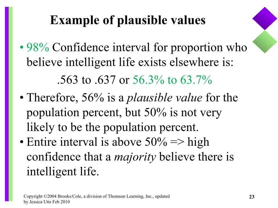
Example of plausible values

• 98% Confidence interval for proportion who believe intelligent life exists elsewhere is:

.563 to .637 or 56.3% to 63.7%• Therefore, 56% is a plausible value for the

population percent, but 50% is not very likely to be the population percent.

• Entire interval is above 50% => high confidence that a majority believe there is intelligent life.


24

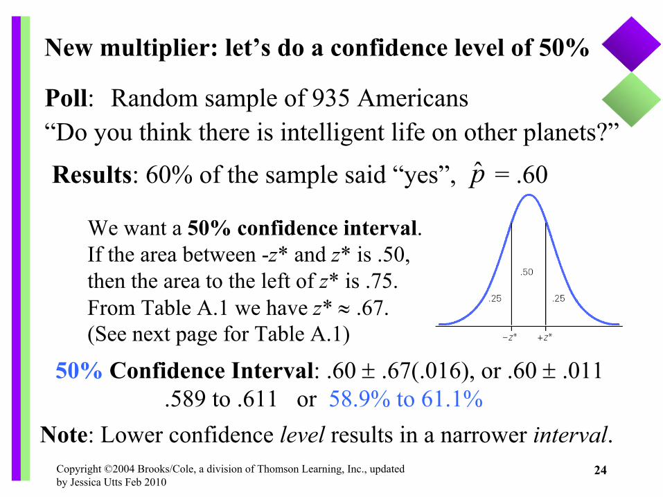
New multiplier: let’s do a confidence level of 50%

Poll: Random sample of 935 Americans“Do you think there is intelligent life on other planets?”

Note: Lower confidence level results in a narrower interval.

Results: 60% of the sample said “yes”, = .60

50% Confidence Interval: .60 ± .67(.016), or .60 ± .011.589 to .611 or 58.9% to 61.1%

p̂

We want a 50% confidence interval. If the area between -z* and z* is .50, then the area to the left of z* is .75. From Table A.1 we have z* ≈ .67. (See next page for Table A.1)

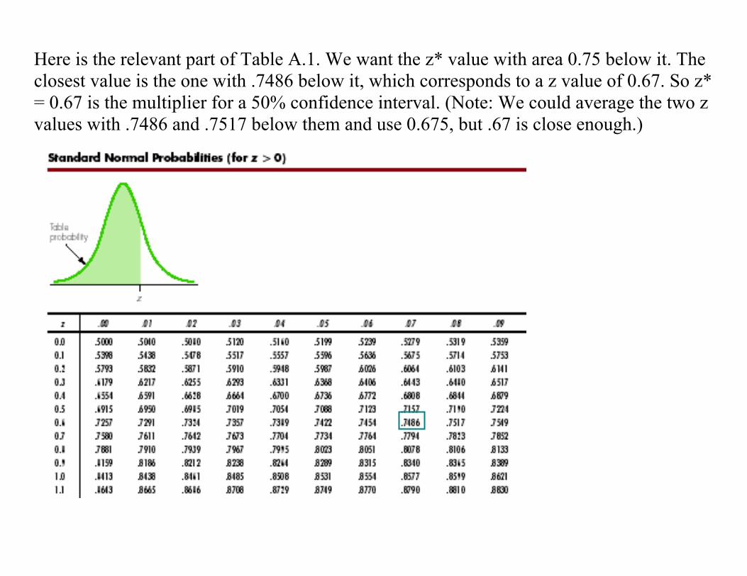
Here is the relevant part of Table A.1. We want the z* value with area 0.75 below it. The closest value is the one with .7486 below it, which corresponds to a z value of 0.67. So z* = 0.67 is the multiplier for a 50% confidence interval. (Note: We could average the two z values with .7486 and .7517 below them and use 0.675, but .67 is close enough.)


25

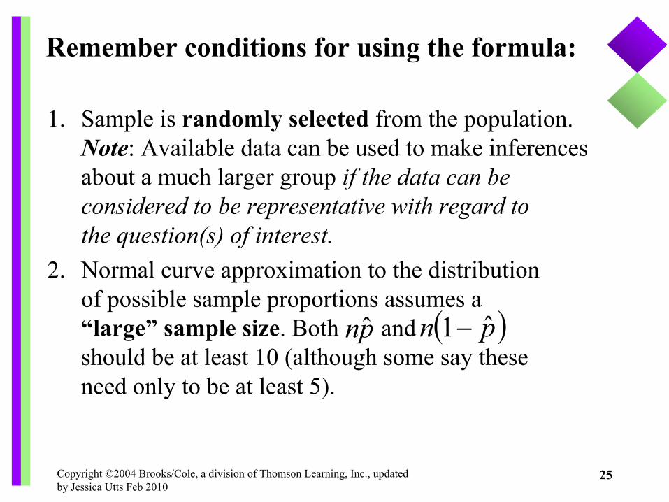
Remember conditions for using the formula:

1. Sample is randomly selected from the population.Note: Available data can be used to make inferences about a much larger group if the data can be considered to be representative with regard to the question(s) of interest.

2. Normal curve approximation to the distribution of possible sample proportions assumes a “large” sample size. Both and should be at least 10 (although some say these need only to be at least 5).

pnˆ ( )pn ˆ1−


26

General CI for p:

In Summary: Confidence Interval for a Population Proportion p

( )n

ppzpˆ1ˆˆ −

± ∗

Approximate 95% CI for p:

( )n

pppˆ1ˆ

2ˆ −±

Conservative 95% CI for p: n

p 1ˆ ±


27

Section 10.4: Comparing two population proportions

• Independent samples of size n1 and n2• Use the two sample proportions as data.• Could compute separate confidence intervals

for the two population proportions and see if they overlap.

• Better to find a confidence interval for the difference in the two population proportions,


28

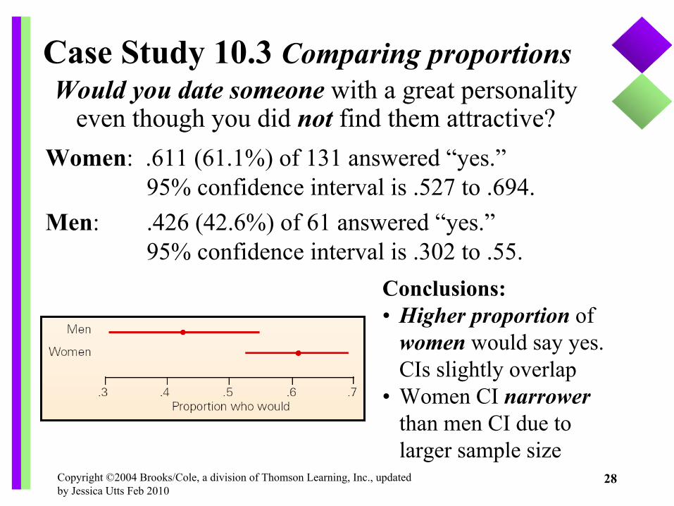
Case Study 10.3 Comparing proportionsWould you date someone with a great personality

even though you did not find them attractive?Women: .611 (61.1%) of 131 answered “yes.”

95% confidence interval is .527 to .694.Men: .426 (42.6%) of 61 answered “yes.”

95% confidence interval is .302 to .55.Conclusions:• Higher proportion of

women would say yes.CIs slightly overlap

• Women CI narrowerthan men CI due to larger sample size


29

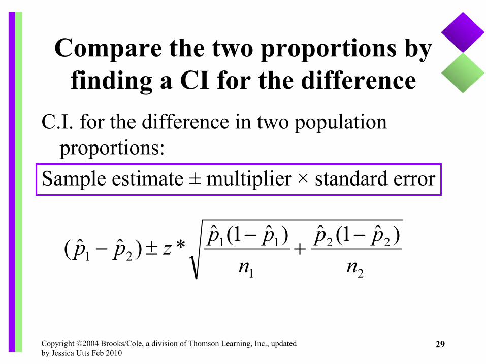
Compare the two proportions by finding a CI for the difference

C.I. for the difference in two population proportions:


2

22

1

1121

)ˆ1(ˆ)ˆ1(ˆ*)ˆˆ(

npp

nppzpp −

+−

±−


30

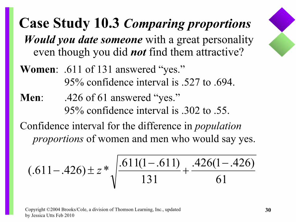
Case Study 10.3 Comparing proportionsWould you date someone with a great personality

even though you did not find them attractive?Women: .611 of 131 answered “yes.”

95% confidence interval is .527 to .694.Men: .426 of 61 answered “yes.”

95% confidence interval is .302 to .55.Confidence interval for the difference in population

proportions of women and men who would say yes.

61)426.1(426.

131)611.1(611.*)426.611(. −+

−±− z


31

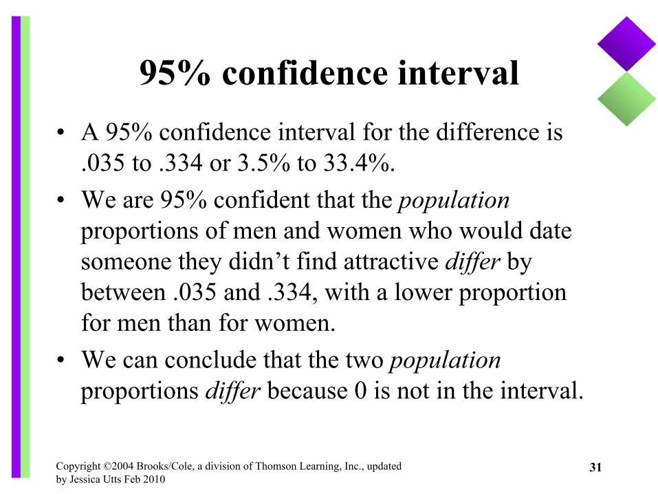
95% confidence interval• A 95% confidence interval for the difference is

.035 to .334 or 3.5% to 33.4%.• We are 95% confident that the population

proportions of men and women who would date someone they didn’t find attractive differ by between .035 and .334, with a lower proportion for men than for women.

• We can conclude that the two populationproportions differ because 0 is not in the interval.


32

Section 10.5: Using confidence intervals to guide decisions• A value not in a confidence interval can be rejected

as a likely value for the population parameter.• When a confidence interval for p1 − p2 does not cover

0 it is reasonable to conclude that the two population values differ.

• When confidence intervals for p1 and p2 do not overlap it is reasonable to conclude they differ, but if they do overlap, no conclusion can be made. In that case, find a confidence interval for the difference.

33

From the Midterm 2 review sheet for Chapter 10 - you should know these now

1. Understand how to interpret the confidence level2. Understand how to interpret a confidence interval3. Understand how the sampling distribution for leads to

the confidence interval formula (pg. 417-418)4. Know how to compute a confidence interval for one

proportion, including conditions needed.5. Know how to compute a confidence interval for the

difference in two proportions, including conditions needed.6. Understand how to find the multiplier for desired

confidence level.7. Understand how margin of error from Chapter 3 relates to

the 95% confidence interval formula in Chapter 108. Know the general format for a confidence interval for the 5

situations defined in Chapter 9 (see summary on page 483).

p̂

announcements - university of california, irvinejutts/8/lecture20.pdfannouncements: •discussion...

Documents