annex ii task 1.1 generic and site-related wave energy data

AANNNNEEXX IIII TTaasskk 11..11 GGeenneerriicc aanndd SSiittee--rreellaatteedd WWaavvee EEnneerrggyy DDaattaa

SSeepptteemmbbeerr 22001100

IEA OES|Oc ean Energy Systems

Ocean Energy Systems

IEA | OES

A report prepared by the RAMBOLL and LNEG to the OES-IA

under the Annex II – Guidelines for Development and Testing of

Ocean Energy Systems

September 2010 OES-IA Document nº T02-1.1

Generic and Site-related Wave Energy Data Final Technical Report OES-IA Document No: T02-1.1 Author(s) Kim Nielsen Ramboll, Denmark & Teresa Pontes LNEG, Portugal

Customer

This report was prepared to the OES IA under ANNEX II: Guidelines for Development and Testing of Ocean Energy Systems Task 1.1 Generic and Site-related Wave Energy Data

Disclaimer The OES IA, whose formal name is the Implementing Agreement for a Co-operative Programme on Ocean Energy Systems, functions within a framework created by the International Energy Agency (IEA). Views, findings and publications of the OES IA do not necessarily represent the views or policies of the IEA Secretariat or of all its individual member countries. Neither the authors nor the organizations participating in or funding the OES IA make any warranty or representations, expressed or implied, with respect to use of any information contained in this report, or assumes any liabilities with respect to use of or for damages resulting from the use of any information disclosed in this document.

Availability of Report

A PDF file of this report is available at: www.iea-oceans.org

Suggested Citation

The suggested citation for this report is: K. Nielsen & T. Pontes (2010) Report T02-1.1 OES IA Annex II Task 1.2 Generic and Site-related Wave Energy Data.

http://www.iea-oceans.org/�

Report 02-1.1 OES-IA Annex II Task 1.1

1

Annex II Task 1.1 Generic and Site-related Wave Energy Data Kim Nielsen, Ramboll & Teresa Pontes, LNEG March 2010 (Revision 3, September 3, 2010)


2

Table of Contents

1 Introduction 3

2 Acknowledgement 3

3 Generic and Site Specific Wave Energy Data 4 3.1 The Global Wave Energy Resource 4 3.2 The Nature of Wind-Generated Ocean Waves 5

4 Generic Ocean Wave Data 7 4.1 Data Preparation and Presentation 12 4.2 Data from Haltenbanken Norway 13 4.3 Data from AUK in the North Sea 14 4.4 Danish Part of North Sea Wave Power Levels 15 4.5 Atlas of UK Marine Renewable Energy Resources 16

4.5.1 Design Wave Height Mapping in the United Kingdom 17 4.6 Belmullet Ireland 18 4.7 Lisboa Portugal 19

5 Data from Wave Test Sites 20 5.1 Guideline for Test Site Information 22

5.1.1 Site Host Address and Contact Details 22 5.1.2 Site Location & Infrastructure 22 5.1.3 Grid Connection 22 5.1.4 Water Depth and Seabed Conditions 22 5.1.5 Distance to Shore 22 5.1.6 Design Wave Data 22 5.1.7 Design Wind Data 22 5.1.8 Design Current Data 22 5.1.9 Design Water Level Variation 22 5.1.10 Joint Probability Diagram (Scatter Diagram) 23 5.1.11 Additional information 23

6 Specific Wave Energy Test Site Data 24 6.1 Pilot Zone, S. Pedro Muel, Portugal 25 6.2 Test Sites in Denmark 27

6.2.1 Nissum Bredning 27 6.2.2 Hanstholm 29

6.3 Test Sites in the United Kingdom 31 6.4 European Marine Energy Centre (EMEC) 31 6.5 Wave Hub 33 6.6 Galway Bay, Ireland 34 6.7 Biscay Marine Energy Platform (bimep), Spain 36 6.8 Port Kembla, Australia 38

7 Bibliography 40


3

1 Introduction

The first part of Annex II was completed in 2003(1), focussing on tank test facilities and methodologies for testing wave power systems in model scales. In 2007 Annex II was extended to focus on guidelines for open sea testing of wave energy converters. Task 1.1 of the extended Annex II proposes wave data to be used as reference data for preliminary evaluation and economic assessment of wave energy converters. Locations are chosen in the northern, middle and southern parts of the North-eastern Atlantic Ocean, as well as the fetch-limited North Sea. The offshore data presented will provide an upper estimate of the energy that can be produced in these areas compared to near shore data at specific locations, where directionality needs to be taken into account. However, the chosen data reflect different ocean conditions, which are seen from the presented bi-variate distributions of significant wave height (Hs) and energy period (Te). Guidelines for site-specific data that will enable designers to evaluate the dimensions and resources at a specific test site are given. Examples of available data relating to selected test sites for testing Wave Power Converters are provided. Each site has different information available, which is presented in different formats. The study has its main focus and most examples from Europe, but the methodology presented can be applied to any ocean area of the world. 2 Acknowledgement

The authors gratefully acknowledge the discussions and input from Fred Gardner, Jens Peter Kofoed, Jose Luis Villate Martinez, Tony Lewis and his team and Tom Denniss, as well as the financial contribution from the Danish Energy Agency, Ramboll and LNEG.


4

3 Generic and Site Specific Wave Energy Data

3.1 The Global Wave Energy Resource Wave energy is a global resource as shown on the world map in Figure 1. The annual power levels range from 5kW/m in sheltered and closed seas and in tropical regions - to more than 60 kW/m in oceanic areas, such as found in the northern and southern hemispheres. The map shows that the oceans are most energetic at latitudes at about 50-60 deg. The blue and green colours indicate power levels below 20 kW/m and the yellow, red and brown colours indicate power levels above 20 kW/m up to more than 60 kW/m.

Figure 1 Ocean Wave Energy resource indicated in kW/m "The data originate from the ECMWF (European Centre for Medium-Range Weather Forecasts) WAM model archive

and are calibrated and corrected (by OCEANOR) against a global buoy and Topex satellite altimeter database."

The highest power levels more than 60 kW/m are found offshore along the coastlines of southern Chile, Africa, Australia, New Zealand, Northwest Canada, west of Scotland (UK) and Ireland. The data presented on Figure 1 are based on 10-year / 6-hourly time-series of wave energy at each point, the model data being validated and calibrated against 10 years of Topex satellite altimeter data for each point, as well as buoy data where available. The points are all offshore and do not reflect the coastal wave climate, which will normally be very different due to various shallow water effects and coastal sheltering. Different software can be used to derive the near shore wave climate from open-ocean, e.g., the Worldwaves package, as well as various shallow-water models such as the SWAN model. In addition to wave power levels, other design criteria are important such as the maximum wave height, design current and wind velocity, the intervals between storms (for maintenance and installation), the water depth and water level variations from tidal action and storm surges and the distance to the coast and infrastructure for installation of devices and power transmission.


5

Information such as seasonal wave power maps (variation of energy through the year) and maps of the ratio of average wave height (this is indicative of the income from a wave power device) and the extreme wave height (indicating the design costs for the wave power plant - or the expenditure) can be obtained from the database. The areas of the world with a good stable resource and low extremes can also be pinpointed using the global database WorldWaves data/OCEANOR/ECMWF. 3.2 The Nature of Wind-Generated Ocean Waves Ocean waves are generated by winds blowing over its surface. If the wind is blowing from the shore, one will observe that initially waves are just ripples; with a trained eye from the ripples you can assess the strength and direction of the wind. Imagine you sit in a boat drifting with the wind further and further to shore. You will observe that the waves are growing in height and length; short waves break as they become too steep and form longer waves that travel faster. After drifting to a certain distance (fetch) the waves do not become larger – they have reached equilibrium with the wind speed and the sea is said to be “fully developed”. The Energy Spectrum of fully developed sea was proposed by Pierson & Moskowitz(2) expressed by the wind speed (U). measured 19.5 metres above the sea level as:

𝑆(𝑓,𝑈) = 𝛼(2𝜋4)

𝑔2𝑓−5𝑒−𝛽�𝑓(𝑈)𝑜𝑓 �

4

(1)

where the constants involved are 𝛼 = 0,0081 𝛽 = 0,74 𝑓(𝑈)0 =

𝑔2𝜋𝑈

Later variations of this spectrum have been used to describe the energy distribution in frequency in an irregular sea surface. Also spreading functions f(θ) have been proposed.

S(f,θ)=S(f)*f(θ) (2)

More information on the spectra and their derivatives can be found in the Annex II report from 2003, (1). For practical purposes, the sea state is characterized by the energy period Te and the significant wave height Hs and the mean direction of propagation. In deep water, the global power level (from all directions) of a sea state is given by:

𝑃𝑤(𝐻𝑠 ,𝑇𝑒) = 𝜌𝑔2

64𝜋𝐻𝑠2𝑇𝑒 ≅ 0,49𝐻𝑠2𝑇𝑒 (3)

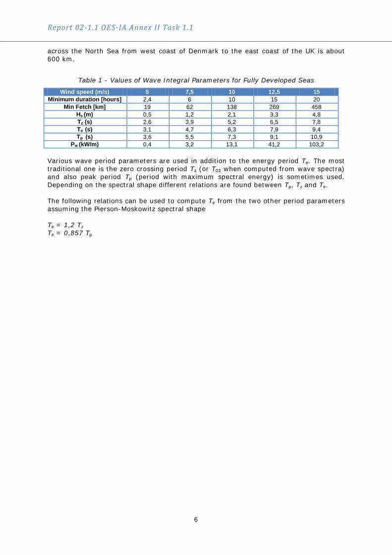
Pw is expressed in (kW/m) if the significant wave height (Hs) is expressed in metres and the energy period (Te) in seconds. Table 1 below indicates at different wind speeds the corresponding significant wave height, periods and power levels for fully developed seas, as well as the minimum fetch and duration required to generate fully developed seas. For comparison the distance


6

across the North Sea from west coast of Denmark to the east coast of the UK is about 600 km.

Table 1 - Values of Wave Integral Parameters for Fully Developed Seas

Wind speed (m/s) 5 7,5 10 12,5 15 Minimum duration [hours] 2,4 6 10 15 20

Min Fetch [km] 19 62 138 269 458 Hs (m) 0,5 1,2 2,1 3,3 4,8 Tz (s) 2,6 3,9 5,2 6,5 7,8 Te (s) 3,1 4,7 6,3 7,9 9,4 Tp (s) 3,6 5,5 7,3 9,1 10,9

Pw (kW/m) 0,4 3,2 13,1 41,2 103,2 Various wave period parameters are used in addition to the energy period Te. The most traditional one is the zero crossing period Tz (or T02 when computed from wave spectra) and also peak period Tp (period with maximum spectral energy) is sometimes used. Depending on the spectral shape different relations are found between Tp, Tz and Te. The following relations can be used to compute Te from the two other period parameters assuming the Pierson-Moskowitz spectral shape Te = 1,2 Tz Te = 0,857 Tp


7

4 Generic Ocean Wave Data

Generic wave data for wave energy systems evaluation was discussed in the first Workshop of the CA-OE project (Coordinated Action on Ocean Energy, EC Contract Contract N°: 502701, 2004-2007) in Aalborg in March 2005. Teamwork Technology presented the wave data information from WERATLAS(3) and showed how four different zones could be defined. The generic scatter diagrams are described in the paper presented at the 6th EWTEC conference in Glasgow in 2006(4). It appears that there are specific trends in terms of the energy content in the waves and typical annual distribution of Te and Hs in different areas of the North-eastern Atlantic. The wave energy resource is generated by the wind and the wind fields are related to the depressions passing from west to east. Ireland and the UK are more frequently hit by strong depressions compared to more southern regions like Portugal. To illustrate the trends four different locations have been chosen as illustrated on the Google map below. The locations are: 1. North-eastern North Atlantic, Norwegian Sea, Haltenbanken, Norway, 42 kW/m 2. Fetch limited conditions as in the North Sea, AUK, 20 kW/m 3. North-eastern Central Atlantic conditions Belmullet, Ireland, 72 kW/m 4. South Atlantic conditions illustrated by Lisboa, PT, 37 kW/m

Figure 2 The four locations chosen in order to show generic trends in the distribution of sea states and their Wave Energy contribution.


8

The highest average power level is found in the Atlantic Ocean west of Ireland and off Scotland (UK), it being higher than 70 kW/m. In the most northern and southern European Atlantic sites, power levels are found to be of similar magnitude (around 40 kW/m). However, the distribution of wave period shows that waves of longer periods are more common at the Lisboa location compared to Haltenbanken in Norway. The power levels around 20 kW/m occur in the fetch limited central region of the North Sea where wind-sea is predominant thus shorter wave periods are found. The annual distribution of energy period Te at the four selected sites is shown on the Figure 3 below (all directions).

Figure 3 Distribution of energy periods at the four sites

To evaluate the relationship between significant wave height Hs and the average energy period Te, the best linear fit between Hs and average Te ave has been determined from the scatter diagrams (in WERATLAS) for each site as follows: Te ave = A*Hs + B [sec] The position of the site, the annual average power level and the four distinct relations between average Hs and Te ave are shown in Table 2, as well as the respective period of observations.

Table 2 Key data from four selected sites

Location Position Pave (kW/m)

Te ave Observation period

Haltenbanken, Norway 65,1° N, 7,4° E 42 0,75*Hs + 5,65 1980 - 88 AUK, North Sea 56,23° N, 2,03° E 20 0,75*Hs + 4,98 1984 - 94 Belmullet,Ireland 54° N, 12° W 72 0,90*Hs + 6,34 1987 - 94 Lisboa, Portugal 39° N, 12° W 37 1,09*Hs + 6,47 1987 - 94

Distibution of Energy Periods

0

50

100

150

200

250

300

2,5 3,5 4,5 5,5 6,5 7,5 8,5 9,5 10,5 11,5 12,5 13,5 14,5 15,5

Te Sec.

Parts

per

thou

sand

s

LisboaBelmulletNorth SeaHaltenbanken, NO


9

The relations between Hs and Te ave are plotted on a common graph shown on Figure 4.

Figure 4 - Linear Relationship between Hs and Te ave for the Selected Sites

In Figure 4 it should be noted that the average energy period is about 2 to 3 seconds larger at the Lisboa site compared to the North Sea site for the same significant wave height Hs. This is due to the fact that in the North Sea wind-sea conditions are dominant, while in Lisboa swell prevails. It appears from Figure 4 that different linear relations can be used to describe the most likely wave energy period Te for the different locations as a function of the significant wave height Hs. Such relations can be useful, e.g., if it is desired to present and evaluate the most likely performance curve of a wave power converter based on its performance matrix. In this way the three-dimensional performance matrix is simplified to a two dimensional power curve related to a generic location.

Average relation between Hs and Te ave

0

1

2

3

4

5

6

7

8

9

10

11

12

13

0 1 2 3 4 5 6

Hs [m]

Te a

ve [s

ec]

Te ave, Lisboa, PT

Te ave, Belmullet UK

Te ave, Haltenbanken, NO

Te ave, North Sea


10

Figure 5 - Annual Distributions of Hs (hours per year) for the Four Selected Sites

In Figure 5 sea states with Hs between 1,5 meter and 2,5 meter occur at all sites for more than 2,500 hours per year. Sea states with Hs between 2,5 meter and 3,5 meter occur more than 1,500 hours per year. At the Lisboa site and in the North Sea, the significant wave height Hs exceeds 5,5 meter about 125 hours per year (5 days per year). In the north, at Haltenbanken in the Norwegian Sea, this level is exceeded more than 500 hours per year (20 days per year) and at the Belmullet site more than 1,000 hours per year (41 days per year).

Annual Distribution of Hs

0

500

1000

1500

2000

2500

3000

3500

4000

Hs Meter

Hours / year

North Sea 272 3224 2742 1480 631 254 123

Haltenbanken, NO 18 2059 2786 1708 1060 552 526

Belmullet UK 0 1077 2751 1875 1226 788 1007

Lisboa, PT 0 1586 3513 2234 894 368 131

< 0,5 0,5 - 1,5 1, 5 - 2,5 2,5 - 3,5 3,5 - 4,5 4,5 - 5,5 >5,5


11

Figure 6 - Annual Energy Contribution for each Sea State at the Four Locations.

Figure 6 shows the annual energy contribution from each sea state characterized by Hs, and one can notice that up to Hs = 3,5 meter the wave conditions at Lisboa provide most energy. For sea states with Hs above 3,5 metres the north and central East-Atlantic locations Haltenbanken and Belmullet respectively provide most energy. Further almost half of the energy at Belmullet comes from seas states above 5,5 metres. Tables 3 to 6 below show how many hours per year five sea states (Hs from 1 metre to 5 metres) occur and for each Hs, the most likely energy period Te and the energy contribution per meter per year.

Table 3 - Haltenbanken Norway

Hs [m] 1 2 3 4 5 >5,5 Total Energy period Te [sec] 6,40 7,16 7,91 8,66 9,41 >9,79 Hours per year 2059 2786 1708 1060 552 526 8707 Energy [kWh/m/year] 8228 40079 61155 73389 64226 128877 375957

Table 4 - North Sea (AUK)

Hs [m] 1m 2m 3m 4m 5m >5,5m Total Energy period Te [sec] 5,73 6,47 7,22 7,96 8,71 >9,08 Hours per year 3224 2742 1480 631 254 123 8725 Energy [kWh/m/year] 10233 35737 48198 39296 27097 22153 182757

Table 5 – Belmullet, Ireland


Table 6 - Lisboa, Portugal


Energy contributions from sea states

0

50000

100000

150000

200000

250000

300000

350000

Hs meter

kWh/y/m

Haltenbanken, NO 3 8228 40079 61155 73389 64226 128877

North Sea 43 10233 35737 48198 39296 27097 22153

Belmullet UK 0 5859 44836 75443 98358 105514 311718

Lisboa, PT 0 8857 61559 97729 76228 52473 29154

< 0,5 0,5 - 1,5 1, 5 - 2,5 2,5 - 3,5 3,5 - 4,5 4,5 - 5,5 >5,5


12

4.1 Data Preparation and Presentation The wave data analysed have been obtained from the WERATLAS (3). Data for Belmullet and Lisboa are results from the ECMWF wind-wave WAM model, covering an 8-year period (1987-1994); for AUK (North Sea) and Haltenbanken, buoy data were used covering 1980-1988 and 1983-1994, respectively. The wave data analysed refers to all directions. For each location a scatter table of Hs and Te is shown. Each cell represents an interval that for the energy period Te spans over 1 second and for Hs is 0,5 metre. The value in each cell shows the relative frequency of occurrence of the respective combination (Hs, Te). For each row of Hs the average energy period Te ave is calculated and shown in the column (Te ave) this value is the most likely energy period associated with the value of Hs. Central values of Hs and Te for each bin are used assuming an even distribution within each bin. The probability of each row is shown representing a specific level of Hs is shown in the column (sum), the accumulated probability in column (Acc) and the power contribution from this level of Hs in column (dP). Summing up the power contributions (dP) for each row an estimate of the power resource in kW/m at the site is obtained as a sum of the column (dP). A plot of the average energy period Te as a function of Hs is shown below at the corresponding scatter table. A trend line giving the best linear fit between the plotted points is shown; from the corresponding formula the linear coefficient and constant has been derived as showed for all sites in Table 2. The probability of occurrence in each bin is given in parts per thousands without decimal points. This can be seen as the sum of occurrence is not 1,000. In the WEARATLAS the decimals are included when calculating the power levels for the four sites and this gives rise to slightly different values as shown in the table below. For practical purpose this difference is of minor importance.

Table 7 Comparison between calculations based on the truncated information to the original source WERATLAS

Location WERATLAS Pave (kW/m)

This Report Pave (kW/m)

Haltenbanken, Norway 42 42 AUK, North Sea 21 20 Belmullet,Ireland 75 72 Lisboa, PT 39 37


13

4.2 Data from Haltenbanken Norway

Figure 7 - Plot of the Average Energy Period Te Ave as a Function of the Significant Wave Height Hs, including the Linear Trend Line (In Black) fitted to the Data for Haltenbanken,

Norway.

Bivariate Frequency Table of (Hs,Te)

LOCATION: ATL.37 HALTENBANKEN ( 65,1° N ; 7,4° E ) DATA: Directional spectra from buoy measurements (1980 - 1988)SEASON: Annual

Hs\Te 2,5 3,5 4,5 5,5 6,5 7,5 8,5 9,5 10,5 11,5 12,5 13,5 14,5 15,5 sum Acc Te ave dP0,25 1 1 2 2 6,00 0,000,75 9 28 24 9 2 1 73 75 6,09 0,121,25 11 53 57 28 10 3 162 237 6,39 0,801,75 2 36 57 47 22 5 2 171 408 6,93 1,792,25 14 51 44 25 9 3 1 147 555 7,34 2,702,75 2 27 37 27 12 4 1 110 665 7,83 3,213,25 11 32 24 11 4 2 1 85 750 8,21 3,643,75 2 22 24 13 5 2 1 69 819 8,60 4,124,25 11 21 13 5 2 52 871 8,85 4,104,75 3 14 11 4 2 1 35 906 9,24 3,605,25 1 10 10 5 1 1 28 934 9,43 3,595,75 4 7 4 2 1 18 952 9,89 2,906,25 2 6 3 1 1 13 965 9,96 2,506,75 4 3 1 8 973 10,13 1,827,25 3 3 1 7 980 10,21 1,857,75 1 3 1 5 985 10,50 1,568,25 3 1 4 989 10,75 1,448,75 1 1 2 991 11,00 0,839,25 1 1 2 993 11,00 0,939,75 0 993 0,00

10,25 1 1 994 11,50 0,6010,75

sum: 0 0 22 134 230 234 185 109 53 21 6 0 0 0 994 42,11

Haltenbanken, NO

y = 0,7514x + 5,6523

0,00

2,00

4,00

6,00

8,00

10,00

12,00

0 1 2 3 4 5 6

Hs meter

Te a

ve s

ec


14

4.3 Data from AUK in the North Sea

Figure 8 Plot of the average energy period Te ave as a function of the significant wave height Hs, including the linear trend line (in black) fitted to the data for AUK, North Sea.


LOCATION: ATL.32 AUK ( 56,23° N ; 2,03° E ) DATA: Directional spectra from buoy measurements (1984 - 1994)SEASON: Annual

Hs \ Te 2,5 3,5 4,5 5,5 6,5 7,5 8,5 9,5 10,5 11,5 12,5 13,5 14,5 15,5 Sum Acc Te ave dP0,25 4 14 7 4 2 31 31 5,05 0,000,75 9 64 56 23 10 6 2 1 171 202 5,45 0,261,25 38 93 41 15 7 2 1 197 399 5,84 0,891,75 2 75 64 21 9 4 1 176 575 6,36 1,692,25 23 76 25 8 4 1 0 137 712 6,75 2,312,75 2 49 32 10 4 1 1 99 811 7,22 2,673,25 19 38 9 3 1 0 0 70 881 7,49 2,733,75 3 27 12 2 1 0 0 45 926 7,86 2,454,25 13 12 2 0 0 27 953 8,09 1,954,75 3 11 2 1 0 0 17 970 8,56 1,625,25 1 8 3 0 0 0 12 982 8,67 1,415,75 3 3 1 0 0 7 989 9,21 1,056,25 1 2 1 0 0 4 993 9,50 0,736,75 1 1 2 995 10,00 0,457,25 1 0 0 1 996 9,50 0,257,75

0 13 118 256 279 187 96 35 11 1 0 0 0 0 996 20,47

AUK, North Sea

y = 0,7453x + 4,9804

0,00

1,00

2,00

3,00

4,00

5,00

6,00

7,00

8,00

9,00

10,00

0 1 2 3 4 5 6

Hs [m]

Te a

ve [s

]


15

4.4 Danish Part of North Sea Wave Power Levels Typical wind generated waves within a sea area of limited fetch are found in the North Sea, the Baltic Sea and in the Mediterranean. In these areas the power levels vary between 5 and 20 kW/m. The Danish part of the North Sea has been investigated in great detail, using numerical wind-wave models calibrated with wave measurements at the Gorm Oil production field and also using measurements at Fjaltring, th is closer to shore. Data have been extracted in six data points that are represented the map below enabling in this way to show how the wave power levels and design waves vary within the borders of the Danish part of the North Sea. The data are given in Table 7 below.

Figure 9 Map showing Six Selected Points in the Danish Part of the North Sea(5) It is estimated that if a 200 km-long line of wave power converters were deployed along the north-south direction and 25% of the wave power could be converted this could cover about 20% of the Danish electricity consumption (5).

Table 8 - Wave Data at the six points shown in Figure 9

Location Average Wave Power

Distance to shore

Water depth

50 years Design

(kW/m)

(km)

(m)

Hs (m)

Tp (s)

Point 1 7 64 20 5,7 10,0 Point 2 12 100 31 8,4 12,1 Point 3 16 150 39 9,6 12,9 Point 4 17 150 40 9,3 12,7 Point 5 14 100 58 11,4 14,1 Point 6 11 68 166 10,6 13,6 Fjaltring 7 4 20 6,4 10,5 Ekofisk 24 300 71 12,6 14,8

0 50 100 150 km

5030

NORWAY

DENMARK

DENMARKGERMANY

50

30

Fjaltring

5

6

4

3

1

Denmark

30

Ekofisk

Gorm C

2


16

4.5 Atlas of UK Marine Renewable Energy Resources

Figure 10 - Variation of Wave Power Levels (in kW/m) around UK

In Figure 10 one can observe that the power level varies from more than 70 kW/m at large distances from the Scottish west coast until 15 - 20 kW/m, as the coast is approached(6).


17

4.5.1 Design Wave Height Mapping in the United Kingdom The power level is influenced by the location the same happens with the design wave height. A study has been carried out also to map the variation in design wave heights in UK waters such as found in (7), the 100-year Hs contour map being presented in Figure 11.

Figure 11 – 100-year Hs contour map (Reproduced under the terms of the Click-Use Licence). Important note: the information displayed on this map is intended as a guide

and should not be treated as a substitute for site-specific study.(7)


18

4.6 Belmullet Ireland

Figure 12 - Plot of the average energy period Te ave as a function of the significant wave height Hs, including the linear trend line (in black) fitted to the data for Belmullet,

Ireland


LOCATION: ATL.23 BELMULLET ( 54° N ; 12° W ) DATA: Directional spectra from WAM (1987 - 1994)SEASON: Annual

Hs \ Te 2,5 3,5 4,5 5,5 6,5 7,5 8,5 9,5 10,5 11,5 12,5 13,5 14,5 15,5 Sum Acc Te ave dP0,25 0 0 0,000,75 1 5 6 1 13 13 7,04 0,031,25 8 28 44 23 7 110 123 7,44 0,631,75 8 38 48 45 24 5 168 291 7,82 1,982,25 1 28 37 30 33 14 3 146 437 8,32 3,032,75 7 34 30 25 18 6 1 121 558 8,79 3,963,25 1 16 28 20 18 9 1 93 651 9,24 4,473,75 0 4 21 17 15 12 5 1 75 726 9,89 5,144,25 1 14 19 14 10 5 2 65 791 10,13 5,864,75 0 4 15 14 10 5 3 51 842 10,62 6,025,25 0 1 9 13 9 4 2 1 39 881 10,91 5,785,75 0 3 11 9 5 2 1 31 912 11,34 5,726,25 2 7 6 5 2 1 23 935 11,54 5,116,75 4 5 4 2 1 16 951 11,94 4,297,25 2 4 3 2 1 12 963 12,17 3,787,75 0 1 3 4 2 1 11 974 12,41 4,048,25 2 2 2 1 7 981 12,79 3,008,75 0 1 2 2 1 6 987 13,00 2,949,25 0 0 1 1 2 989 13,00 1,109,75 1 1 1 3 992 13,50 1,90

10,25 0 2 1 3 995 13,83 2,1510,75 1 1 996 14,50 0,8312,75

Sum 0 0 0 18 107 190 197 174 136 89 48 26 11 0 996 71,74


19

4.7 Lisboa Portugal

Figure 13 - Plot of the Average Energy Period Te ave as a Function of Significant wave height Hs, including the linear trend line (in black) fitted to the data for Lisboa, Portugal.


LOCATION: ATL.13 LISBOA ( 39° N ; 12° W ) DATA: Directional spectra from WAM (1987 - 1994)SEASON: Annual

Hs \ Te 2,5 3,5 4,5 5,5 6,5 7,5 8,5 9,5 10,5 11,5 12,5 13,5 14,5 15,5 Sum Acc Te ave dP0,25 00,75 1 6 7 2 1 17 17 7,26 0,031,25 9 38 63 41 12 1 164 181 7,57 0,961,75 7 45 46 48 36 23 6 1 212 393 8,25 2,642,25 1 29 36 31 31 29 26 5 1 189 582 9,00 4,252,75 7 29 26 23 21 28 16 4 154 736 9,73 5,603,25 0 15 19 16 15 15 14 6 1 101 837 10,16 5,353,75 0 2 13 12 12 7 8 7 2 63 900 10,63 4,654,25 5 9 6 5 6 4 3 1 39 939 11,19 3,894,75 0 2 5 4 6 4 3 3 1 28 967 11,61 3,625,25 0 2 4 2 2 2 1 1 14 981 11,86 2,265,75 0 1 2 2 1 1 1 8 989 11,75 1,536,25 2 1 1 4 993 11,25 0,876,75 1 1 2 995 12,00 0,547,25 1 1 996 12,50 0,327,75

Sum 0 0 0 18 125 198 187 148 119 99 60 28 11 3 996 36,51

Lisboa

y = 1,0859x + 6,4695

0,00

2,00

4,00

6,00

8,00

10,00

12,00

14,00

0 1 2 3 4 5 6

Hs [m]

Te a

ve [s

]


20

5 Data from Wave Test Sites

Since year 2005 the number of ocean test sites proposed and used for testing of wave energy systems has increased significantly. Figure 14 below shows some of the European sites.

Figure 14 - Test Sites for Testing Ocean Energy Systems in Particular Wave Energy Systems [Map provided by HMRC, 2009]

In Portugal the first grid-connected OWC plant was build on the Azores island of Pico, being completed in 1999. The milder climate and, more recently, the favourable feed-in tariff have attracted several wave energy developers to Portugal, pioneered by AWS, followed by Wave Roller and Pelamis. Negotiations with other developers are underway having in view the deployment of their devices in this country. In 2008 a large dedicated area for deployment of prototypes, pre-commercial and commercial wave farms has been defined (the Wave Energy Pilot Zone). One of the first well-established test sites within Europe is the European Marine Energy Centre (EMEC) on the Orkney Islands in Scotland. This site is exposed to the Atlantic waves with strong tidal streams between the Scottish isles. Both tidal and wave energy systems can be tested at EMEC. Marine energy converters like Pelamis (wave energy converter) and OpenHydro (tidal energy converter) have been tested there and the Aquamarine wave power system is currently deployed there. In the UK the Wave Hub in southwestern England is being prepared for testing arrays of wave energy converters. It will be possible to test four different technologies with grid connections at the same time. In contrast to these exposed sites the sheltered site Nissum Bredning in Denmark has become well known from the testing of the Wave Dragon scaled 1:4,5 prototype and the


21

Wave Star scaled 1:10 prototype. In addition an exposed location within Denmark DANWEC has been founded as a Danish wave energy test site in the North Sea off the coast of Hanstholm. A section of a half-scale prototype of the Wave Star is presently being carried out at this location. Data from some of these wave energy test sites including information on power level, water depth and maximum significant wave height is shown on Table 8 below for a selected number of testing sites.

Table 9 - Summary Test Site Data

Site Country Power level

[kW/m]

Water depth

[meter]

Hs max (estimate) [meter]

EMEC UK 21 50 15 Wave Hub UK 17 50-65 14,4

Pilot Zone PT 25 30-90 15,5 (d=30m)

bimep Spain 21 50-90 11,4

Hanstholm DK 6 20 - 30 6,5 Nissum Bredning DK 0,2 5-8 1,2

Galway Bay Ireland 2,4 20-25 5

Port Kembla Australia 6,7 6 7 More detailed data collected from some of these sites are presented in the following sections of this chapter. The data has been collected initially from available data in literature and on the Internet and the available data types were found to vary from site to site. As a consequence some guidelines have been drawn to indicate the typical information that is needed to make a preliminary design of a wave energy converter to a specific site or evaluate the results obtained at a specific site. A questionnaire (8) including these guidelines has been circulated within the OES-IA to obtain information. Some of the information received has been included in this report as examples (Bimep, Galway Bay and Port Kembla). In order to prepare preliminary planning and design of any ocean energy converter for testing at a specific site, the data described in the guidelines below are required. Further, these guidelines will encourage test sites to make such data available, e.g., on their web pages. The summary data presented for various sites are in any case indicative and thus cannot be used in a detailed design study; this will require further information provided by the site, where the tests it is planned to be carried out.


22

5.1 Guideline for Test Site Information In order to obtain comparable information from different wave energy test sites, the guidelines below show what type of information would be helpful to be made publicly available for preliminary planning purposes. 5.1.1 Site Host Address and Contact Details Name and Address: e-mail: Web page: 5.1.2 Site Location & Infrastructure A short description of the site, offices, and permits, including a map indicating the site, the size of the area and the co-ordinates of the location must be given. Ongoing projects and previous project/systems tested should be mentioned. Distance to large town Distance to nearest airport Distance from nearest service port to site Distance from nearest access harbour to site Restrictions, availability & conditions if any 5.1.3 Grid Connection

o On land o Off/shore (at what depth)

Connection voltage and power level 5.1.4 Water Depth and Seabed Conditions Water depth at the site and the seabed material – mud, sand, gravel or rock - is useful for mooring and installation. 5.1.5 Distance to Shore The shortest distance to shore should be indicated as well as the distance to the nearest harbour for maintenance. 5.1.6 Design Wave Data The design wave conditions can be determined based on statistical information. The method used should be indicated as well as the chosen return period (10, 50 or 100 years). In this report the direction from where the (design) wave is coming should be indicated (nautical convention). In more detailed studies directionality is recommended. 5.1.7 Design Wind Data Depending on the freeboard of the wave energy converter, the wind forces can have an impact on the design loads, the maximum wind speed (and most likely direction) with the same return period as the waves should be indicated. 5.1.8 Design Current Data Depending on the submerged part of the wave energy converter, the current forces can have an impact on the design loads; the maximum current speed with the same return period as the waves and wind should be indicated as well as the expected direction. 5.1.9 Design Water Level Variation High and low water conditions can have an impact on the mooring design of the converter; such extreme levels can be indicated relative to the MWL.


23

5.1.10 Joint Probability Diagram (Scatter Diagram) The annual average power level of a given site (all year and all directions) is calculated from a scatter diagram that includes the frequency of occurrence of different combinations of sea states, described by intervals of Te and Hs. Hs - Significant wave height [meter] Te – Energy Period [seconds] or Tz – Zero-crossing Period [seconds] The width of the period intervals (bins) is normally 1 second and for wave height intervals is 0,5 metre or 1 metre, depending on the wave climate (benign test sites for smaller scale testing, such as Nissum Bredning, will be presented with smaller intervals). In each cell the frequency of occurrence can be given in hours per year, in parts per thousands (ppt) and sometimes in percent. Diagrams can also be generated for each month to illustrate the power variation over the year or representing waves coming from different directions. Variation in power from year to year is normal and thus the under laying data must cover a period of more than ten years to provide a fair average estimate.

Table 10 Example of the layout of a Joint probability diagram showing the annual number of hours each combination of Hs and Te prevail.

Energy Period Te or Zero-crossing Period Tz

Hs\T 3,5 4,5 5,5 6,6 7,5 8,5 9,5 10,5 11,5 12,5 13,5 14,5 sum

Si

gnifi

cant

Wav

e H

eigh

t Hs

0,25 0,75 1,25 1,75 2,25 2,75 3,25 3,75 4,25 4,75 5,25 5,75 6,25 6,75 7,25

sum 5.1.11 Additional information Facilities available: Vessels, Cranes, Engineering, Industry Equipment available at site: Wave measurements (yes/no) Wind measurements (yes/no) Water level measurements (yes/no) Current measurements (yes/no) Water/air temperature measurements (yes/no) Can additional information be obtained such as, typical wave spectra, directional spectra, tidal current profiles and turbulence? The guidelines are based on the questions included in the test site questionnaire(8)


24

6 Specific Wave Energy Test Site Data

Specific test sites chosen to be included in this report are shown on the map below except the site at Port Kembla, 100 km south of Sydney, Australia.

Figure 15 - Test Sites along the Atlantic Coast


25

6.1 Pilot Zone, S. Pedro Muel, Portugal Portugal has been able to attract many wave energy companies from abroad due to its favorable wave resource, its mild climate, and attractive testing conditions such as providing permits and favorable feed-in tariffs for produced energy. As such many of the first large scale tests such as the 2 MW Archimedes Wave Swing, tested near Porto in the period 2000 – 2006 (9) and Pelamis prototype tests in 2008 of three 750 kW devices have taken place in Portugal (10), as well as the Finish Wave Roller 2006 – 2007(11). In 2007 it was decided to provide a dedicated area for testing wave energy systems known as the Pilot Zone. Site Location The Pilot Zone is located off the west coast of Portugal about 130 km north of Lisboa, near a village S. Pedro de Muel. The area is about 320 km2. It is planned for demonstration, pre-commercial and commercial exploitation, with a planed maximum grid integration of 250 MW [OES-IA newsletter 12]. Water Depth and Seabed Conditions The pilot zone was defined between 30 and 90 m water depth. In the area sand is abundant; a geological survey is planned. The distance from the 30 m bathymetric to shore is 4,5 km and the 50m bathymetric is 7 km off the coast. Some initial data related to the site are provided below.

Table 11 - Main characteristics of the Wave Energy Pilot Zone

Location: Pilot Zone Portugal 39º54' N 9º06' W Water depth 30 – 90 [m] Design significant wave height Hs (at 30m depth) 11 [m] Design energy period Te (at 30m depth) 19 [sec] Max wind speed 25 [m/s] Max Current speed 3,4 [m/s] Max high water level - (m) Min low water level - (m) Maximum ice thickness - [m] Wave power annual average (50 meter depth) 25 [kW/m]

The scatter diagram in Table 12 is obtained from buoy data 2004 – 2005 at 50 meter water depth. Using the full expression for group velocity taking the water depth into account the annual power calculated is 23,3 kW/m. Correcting this value to the 11-year period (1989 – 1999) the value becomes 25 kW/m as shown in summary Table 11. Using the deepwater approximation for wave power calculation and the one year data shown in the scatter diagram Table 12 the annual wave power average is 21,1 kW/m.

Figure 16 - Pilot Zone in Portugal


26

Table 12 Joint probability diagram from the Pilot Zone in Portugal

References, (OES-IA Test site info provided by LNEG; Teresa Pontes)

Figure 17 - Relationship between Significant Wave Height (Hs) and the average energy

period (Te)

Hs \ Te ≤5 5,5 6,5 7,5 8.5 9.5 10,5 11,5 12,5 13,5 14,5 15,5 ≥17 Sum Te ave dP0,25 1 3 4 5,25 0,000,75 10 26 42 43 14 8 1 1 145 6,90 0,291,25 3 21 41 54 47 41 17 5 229 7,97 1,451,75 8 36 48 47 34 35 17 6 4 235 8,73 3,192,25 15 30 37 36 30 18 7 2 175 9,23 4,152,75 3 18 17 19 19 16 6 1 99 9,61 3,653,25 6 9 8 9 14 6 2 1 55 10,09 2,973,75 1 1 3 6 6 7 3 27 11,28 2,174,25 1 6 3 4 2 16 11,44 1,684,75 1 1 3 1 1 7 11,36 0,915,25 1 1 1 3 11,83 0,505,75 1 1 9,50 0,166,25

≥7Sum 14 58 137 200 174 151 124 83 38 16 0 1 0 996 21,11


27

6.2 Test Sites in Denmark

Figure 18 - Sheltered Test Site in Nissum Bredning and the Test Site in Hanstholm exposed to the North Sea.

Hanstholm is located in the NW part of Denmark at the North Sea with a fetch of about 600km to the west – sheltered by the UK. There is a large harbour, fishing industries and ferry traffic to Norway. During the period 1987–1996, Danish Wave Power Aps carried out experiments with point absorber system, initially with 6 metre diameter buoy - a 40 kW grid connected wave power converter, followed by a second test with a smaller 2,5 metre float, equipped with data collecting equipment, transmitting performance taken over 20 minutes, 6 times per day over a period of six months September 1996 – January 1997(12). One lesson learned from these tests was to start with the smaller scale tests at sea before the large scale. Most recently in September 2009 WaveStar Energy (13) installed a platform including two floats of 5 meter diameter each installed with a generator power of 55 kW. This combined with other wave energy systems planning to install at Hanstholm, has led to the formation of the Danish Wave Energy Center (DanWEC) in Hanstholm(14). The sheltered test site in Nissum Bredning was established in 1999, during the Danish wave energy program(15), as a site for inventors to test their wave energy ideas in real sea waves. It is located in Nissum Bredning with a fetch of about 10 km in direction SW and water depth of about maximum 5-8 meter some 500 meter from shore. 6.2.1 Nissum Bredning The facility includes a 200-meter long bridge, leading from the shore to a water depth of about 3 meter. Several small-scale devices have been tested from this platform, i.e., the Ecofys/Rossen Wave Rotor(16).


28

At some distance from the pier systems like the Point absorber system has been tested at a water depth of 5-6 meter in year 2000, for a period of 3 month(17). The 20 kW WaveDragon prototype was installed in 2003 and connected to the grid. WaveDragon has been in operation on and off since then, also exploring another site approximately 13 km further to the south-east (18), as shown by the lower green arrow on the map (Figure 19).

Since 2006 the Wave Star Energy device was build and installed at the site connected to the pier. The results of the tests of a 5,5 kW device comprising 40 floats of 1-meter diameter are described in (19). The test site is hosted by the Folkecentre for Renewable Energy in Thy(20).

Table 13 - Main Data from Nissum Bredning Site

Location: Nissum Bredning Water depth 3-5 [m] Design significant wave height Hs, 1 year 1,3 [m] Design zero-crossing period Tz, 1 year 4 [sec] Max wind speed 30 [m/s] Max Current speed 3,4 [m/s] Max High Water level 1,6 (m) Min Low Water level -1,5 (m) Maximum Ice thickness 0,15 [m] Wave power annual average 0,2 [kW/m]

Table 14 - Joint Probability Diagram from Nissum Bredning(21)

Hs\ Tp 1,5 1,7 1,9 2,1 2,3 2,5 2,7 2,9 3,1 3,3 3,5 3,7 3,9 Sum Tp ave dP0,05 3,3 11,1 6,6 3,6 2,4 3,3 0,8 0,7 0,7 0,3 0,1 0,1 0,1 33,1 2,00 0,000,15 1,6 2,2 1,4 0,6 0,8 1,4 1,7 1,5 0,8 0,4 12,4 2,47 0,000,25 0,1 1,3 1,1 1,6 1,3 0,4 0,9 0,5 1 0,7 8,9 2,57 0,010,35 0,8 1,3 3,7 1,6 1,2 0,7 1,6 1,6 0,2 12,7 2,80 0,020,45 0,7 2,6 1,9 1,9 0,8 0,4 0,7 0,1 9,1 2,79 0,020,55 1,7 2,5 1,3 1,2 0,5 0,1 7,3 2,81 0,030,65 0,2 1,1 1,5 1 1 0,3 5,1 2,99 0,030,75 0,1 0,2 1,3 0,7 1,8 0,5 4,6 3,33 0,040,85 0,2 0,4 0,3 0,8 1,4 3,1 3,48 0,030,95 0,1 0,1 0,2 0,6 0,9 1,9 3,70 0,031,05 0,1 0,1 0,1 0,4 0,7 3,44 0,011,15 0,1 0,2 0,3 3,57 0,011,25 0 0 0,001,35 0,2 0,2 3,50 0,011,45

3,3 12,8 10,1 6,9 6,6 13,6 9,8 9,8 8,3 6,8 6,9 3,5 1 99,4 0,22

Figure 19 Nissum Breding power levels up to 500 W/m


29

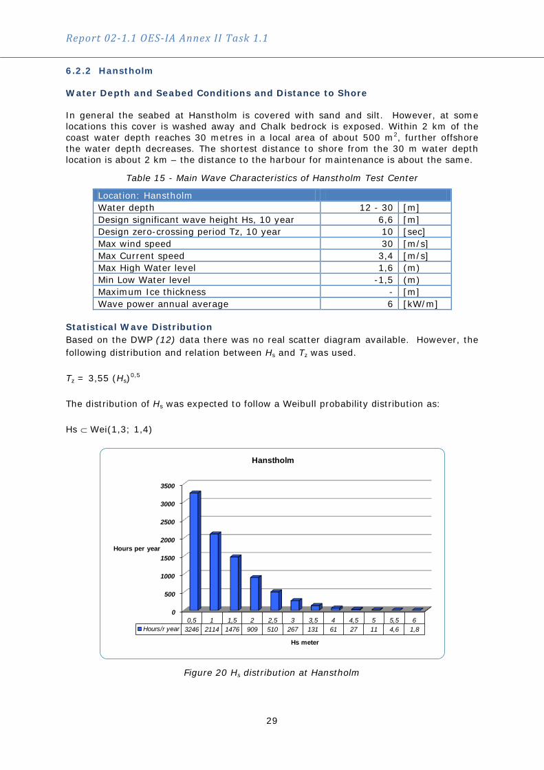
6.2.2 Hanstholm Water Depth and Seabed Conditions and Distance to Shore In general the seabed at Hanstholm is covered with sand and silt. However, at some locations this cover is washed away and Chalk bedrock is exposed. Within 2 km of the coast water depth reaches 30 metres in a local area of about 500 m2, further offshore the water depth decreases. The shortest distance to shore from the 30 m water depth location is about 2 km – the distance to the harbour for maintenance is about the same.

Table 15 - Main Wave Characteristics of Hanstholm Test Center

Location: Hanstholm Water depth 12 - 30 [m] Design significant wave height Hs, 10 year 6,6 [m] Design zero-crossing period Tz, 10 year 10 [sec] Max wind speed 30 [m/s] Max Current speed 3,4 [m/s] Max High Water level 1,6 (m) Min Low Water level -1,5 (m) Maximum Ice thickness - [m] Wave power annual average 6 [kW/m]

Statistical Wave Distribution Based on the DWP (12) data there was no real scatter diagram available. However, the following distribution and relation between Hs and Tz was used. Tz = 3,55 (Hs)0,5 The distribution of Hs was expected to follow a Weibull probability distribution as: Hs ⊂ Wei(1,3; 1,4)

Figure 20 Hs distribution at Hanstholm

0

500

1000

1500

2000

2500

3000

3500

0,5 1 1,5 2 2,5 3 3,5 4 4,5 5 5,5 6Hours/r year 3246 2114 1476 909 510 267 131 61 27 11 4,6 1,8

Hours per year

Hs meter

Hanstholm


30

A recent study (22) completed at AAU has analysed measured wave data from Hanstholm (over the period 01/11/2005 – 25/02/2009) measured at a water depth of 20 metres. Based on the reported data the scatter diagram below has been prepared and it confirms that the average power at Hanstholm is about 6 kW/m. The distribution of Hs compares well to previous assumptions. In the study the period Tmo1 is used and this period is shown to relate to the energy period Te as Tmo1=1,055 Te

Table 16 Joint probability diagram from Hanstholm

Figure 21 Linear Relationship between Hs and Te ave at Hanstholm

Hs\Tmo1 3 3,5 4 4,5 5 5,5 6 6,5 7 7,5 8 8,5 9 >9,5 sum Tmo1ave Te ave dPw hours0,125 0,0050 0,0081 0,0090 0,0048 0,0016 0,0004 0,0003 0,0002 0,0001 0,0001 0,0087 0,039 5,14 5,43 0,00 339

0,5 0,0240 0,0613 0,0677 0,0483 0,0316 0,0172 0,0081 0,0029 0,0016 0,0014 0,0008 0,0007 0,0002 0,0035 0,270 4,31 4,55 0,15 23611 0,0026 0,0161 0,0683 0,0815 0,0621 0,0429 0,0165 0,0056 0,0017 0,0004 0,0001 0,0006 0,298 4,72 4,98 0,73 2614

1,5 0,0001 0,0010 0,0099 0,0524 0,0608 0,0350 0,0156 0,0049 0,0031 0,0006 0,0002 0,0001 0,0002 0,184 5,06 5,34 1,08 16112 0,0003 0,0005 0,0031 0,0365 0,0420 0,0181 0,0046 0,0017 0,0007 0,0004 0,0003 0,0002 0,0001 0,108 5,48 5,78 1,23 950

2,5 0,0003 0,0013 0,0213 0,0220 0,0059 0,0012 0,0005 0,0003 0,0001 0,053 5,85 6,18 1,00 4643 0,0003 0,0002 0,0008 0,0102 0,0127 0,0023 0,0007 0,0004 0,0002 0,0002 0,0003 0,028 6,39 6,74 0,84 247

3,5 0,0002 0,0003 0,0002 0,0043 0,0045 0,0010 0,0003 0,0002 0,0001 0,0001 0,011 6,78 7,15 0,48 994 0,0001 0,0001 0,0001 0,0020 0,0022 0,0002 0,0001 0,005 7,15 7,54 0,29 43

4,5 0,0001 0,0007 0,0010 0,0003 0,0001 0,002 7,53 7,94 0,18 205 0,0002 0,0001 0,0003 0,0003 0,0002 0,0001 0,001 7,89 8,32 0,11 9

5,5 0,0001 0,000 36 0,000 0

6,5 0,0007 0,000

7,5 0,000sum 0,028 0,087 0,155 0,191 0,194 0,160 0,091 0,041 0,018 0,008 0,004 0,002 0,001 0,001 1,000 6,09 8760

y = 0,8534x + 4,107

0,00

1,00

2,00

3,00

4,00

5,00

6,00

7,00

8,00

9,00

0 1 2 3 4 5 6

Te av

e

Hs

Te ave

Linear (Te ave)

Linear (Te ave)


31

6.3 Test Sites in the United Kingdom The UK being exposed to strong ocean waves it has been one of the first countries to realise the potential energy supply that could come from waves. Pioneers like Stephen Salter from the Edinburgh University(23) have inspired a new generation of engineers leading to the formation, i.e., of the team behind Pelamis. Other teams such as the one team at Queen’s University, Belfast (followed by WaveGen) developed in the beginning of 1990 the OWC, leading to the construction of the 500 kW LIMPET device on the shore at the Scottish island of Islay(24). More recently a 300 kW prototype of the nearshore Oyster device (also developed with contribution of Queen´s University) was installed at the EMEC test site on 20 November 2009 (25). 6.4 European Marine Energy Centre (EMEC) The European Marine Energy Centre (EMEC) test facility was established in 2002 to create a North Atlantic test base for both tidal end wave energy devices. Much information is available on the website(26) from EMEC – related to guidelines and preliminary standards. EMEC has contributed the Task 3.3 report on design basis for wave energy converters. The summary data below is extracted from the preliminary survey that was carried out in 2001(27). More detailed data can be obtained from EMEC at a moderate cost.

Figure 22 - Refraction Points used to calculate Nearshore Wave Conditions at 50 metre and 30 metre water depth


32

Table 17 - Main Characteristics of the Billia Croo Wave Site at EMEC Test Centre

Location: EMEC 59.00 N, 3.66W Water depth [m] 50 [m] Design significant wave height Hs 14 -15 [m] Design peak period Tz 14 [sec] Max wind speed [m/s] Max Current speed [m/s] Max High Water level 2,5 (m) Min Low Water level -1,7 (m) Maximum Ice thickness [m] Wave power annual average 21 [kW/m]

Table 18 - Joint probability diagram (Hs andTz) for the EMEC location RP5OS 59,00°N;3,66°W (absolute numbers of occurrences, all directions, all year)

Hs \ Tz <3 3,5 4,5 5,5 6,5 7,5 8,5 9,5 10,5 11,5 12,5 13,5 14,5 Sum Tz ave dP0,25 2653 3618 1943 791 356 250 137 31 2 9781 4,89 0,020,75 2273 9363 5794 2063 734 182 85 40 2 20536 5,05 0,341,25 453 6484 6977 2946 1131 328 106 38 9 7 2 18481 5,48 0,931,75 130 2035 7652 2823 1029 352 139 21 0 5 14186 5,81 1,482,25 288 5405 3838 1081 319 184 66 9 11190 6,20 2,062,75 26 1135 5072 1135 234 137 52 17 2 2 7812 6,65 2,313,25 5 137 3278 2002 250 106 35 19 7 5839 7,01 2,543,75 14 713 2714 415 92 14 9 2 3973 7,49 2,464,25 57 1725 550 94 40 19 0 5 5 2495 7,88 2,094,75 7 430 861 118 26 14 5 1461 8,35 1,625,25 45 767 144 31 5 992 8,68 1,405,75 0 267 255 7 2 5 536 9,05 0,946,25 2 5 54 227 14 5 307 9,35 0,666,75 5 5 142 80 5 237 9,82 0,627,25 66 111 2 179 10,15 0,567,75 31 109 2 2 144 10,33 0,538,25 7 31 21 59 10,74 0,258,75 26 26 52 11,00 0,269,25 2 19 5 26 11,62 0,159,75 14 2 16 11,63 0,10

10,25 7 2 9 11,72 0,0710,75 2 2 12,50 0,0211,25 5 5 12,50 0,0511,75 0

Sum 0 5509 21819 29057 21590 12392 4834 2070 774 197 50 17 9 98318 21,46


33

6.5 Wave Hub The Wave Hub test site is a project in the Southwest of England, located 16 km offshore near Cornwall St. Ives Bay (28)(29)(30). It will be the UK's first offshore facility for demonstration and proving of the operation of arrays of wave energy conversion devices. Up to four different technologies can be placed within a 1 km x 2 km sea area at any one time. This area will be leased to each developer for installation from 2010 onwards. Leases will run for five years, or maybe longer, and will allow each developer to generate a maximum of 4-5 MW of power. Wave Hub will record the incoming waves and will enter into a power purchase agreement on behalf of all developers using the project.

Table 19 Summary data from the Wave Hub.

Location: Wave Hub 50,36° N 5,67° W Water depth [m] 50 [m] Design significant wave height Hs 14,4 [m] Design peak period Tz 14,1 [sec] Max wind speed 33,2 [m/s] Max Current speed 3,8 [m/s] Max High Water level 4 (m) Min Low Water level -4 (m) Maximum Ice thickness - [m] Wave power annual average 17 [kW/m]

Table 20 Joint probability diagram for Wave Hub all directions all year (2005 – 2006)

Hs \ Tz 4,5 5,5 6,5 7,5 8,5 9,5 10,5 11,5 12,5 Sum Tz ave dp0,25 3 9 5 2 190,75 57 95 56 16 2 226 5,66 0,421,25 21 120 69 35 8 3 1 257 6,12 1,441,75 67 80 38 17 6 3 1 212 6,69 2,552,25 11 61 29 14 5 1 121 7,04 2,532,75 27 26 12 3 1 1 70 7,47 2,323,25 3 20 14 5 1 43 8,06 2,153,75 9 11 4 2 26 8,46 1,824,25 1 5 3 1 1 11 9,14 1,074,75 3 2 1 6 9,17 0,735,25 2 3 1 6 9,33 0,915,75 2 1 3 9,83 0,576,25 1 1 9,50 0,22

Sum 81 302 301 176 88 37 13 2 1 1001 16,73


34

6.6 Galway Bay, Ireland The Irish test site at Galway Bay is an Intermediate Scale Test Site (quarter scale Atlantic seas) located at Spiddal, County Galway, Ireland. Two systems have been tested at the site so far:

1. WaveBob (April-May 2006, September-October 2007) (31) 2. OE Buoy (December 2006–August 2007, October 2007–August 2009) (32)

There are no onshore facilities at the site. Individual developers have made their own arrangements for data transmission, etc. Vessels and cranes are available in Galway Docks. A number of engineering companies exist in Galway, one heavy steel fabrication company is located on the Galway Docks site. The site access is pre-permitted with conditions set down by the Marine Institute (33) The most relevant information for this test site follows: Distance to large town – 15km, Distance to nearest airport – 20km, Distance from nearest service port to site – 20km, Distance from nearest access harbour to site – 1,5km, Distance from site to shore – 1km, Restrictions, availability & conditions if any – Access Harbour Tidal – 2 hours either side of high water Water depth at site is about 22m. Tidal range up to 5m (Spring tidal) The seabed material is mud, sand, gravel or rock – sand / mud Wave measurements have taken place since 2005 – directional buoy deployed since end of 2008. During this period the highest sea state was measured on 31 December 2006 with 4,3 meter Hs.

Table 21 – Summary Data for Galway Bay

Location: Galway Bay 43º 28´ 22.6´´ N; 2º 51´ 15.9´´ W Water depth 22 [m] Design significant wave height Hs (estimate) 5 [m] Design peak period Tp (estimate) 10 [sec] Max wind speed NA [m/s] Max Current speed NA [m/s] Max High Water level 2,5 (m,MSL) Min Low Water level -2,5 (m,MSL) Maximum Ice thickness - [m] Wave power annual average 2,4 [kW/m]


35

Figure 23 Sea Conditions in Galway Bay

Table 22 Joint Probability Diagram from Galway Bay

Galway Bay test site: pos 53,228°N; 9,266°WHs\Tz 2,25 2,75 3,25 3,75 4,25 4,75 5,25 5,75 6,25 6,75 7,25 7,75 Sum Tz ave dP

0,25 4,21 9,04 6,66 5,65 5,14 4,38 3,6 2,45 1,3 0,73 0,1 0,02 43,28 3,85 0,060,75 2,48 9,21 8,15 4,41 3,05 2,11 1,2 0,77 0,12 0,05 31,55 3,95 0,411,25 0,36 4,21 6 2,86 0,83 0,45 0,15 0,01 14,87 4,30 0,591,75 0,12 1,72 3,15 0,85 0,17 0,03 0,03 6,07 4,70 0,512,25 0,02 0,85 1,72 0,08 0,01 0,02 2,7 5,11 0,412,75 0,61 0,41 0,01 1,03 5,46 0,253,25 0,28 0,07 0,35 5,85 0,133,75 0,01 0,14 0,15 6,22 0,084,25 0

Sum 4,21 11,52 16,23 18,13 17,29 14,29 9,72 5,05 2,48 0,91 0,15 0,02 100 2,44


36

6.7 Biscay Marine Energy Platform (bimep), Spain The Biscay Marine Energy Platform (bimep) test site is located in the sea off the coast of the village of Armintza, in the municipal area of Lemoiz, some 30 kilometres north of Bilbao in the Basque Country, Spain. Reserved offshore area of 4 x 2 km, marked with navigation buoys. These dimensions include a 500 m guard area between the outer limits of the converter sites and the edge of the reserved area. bimep is expected to start operation in 2011.

Figure 24

bimep will be associated to a marine energy research centre located in the town of Lemoiz. Applications for permits have been handed in according to Spanish legislation. Applications have been submitted for “Consultation for the necessity of Environmental Impact Assessment, Electric installations under special regime, and Occupation of public maritime domain”, so the licensing is now in process. Distance to large town: 30 km Distance to nearest airport: 24 km Distance from nearest service port to site: 10 Nautical Miles [NM] (1NM = 1,852 Km) Distance from nearest access harbour to site: small harbour at 1 NM, bigger ones at 6NM and 10NM. Distance from site to shore: nearest point at 0.54 Nautical mile (NM), distance from closest test berth to shore: 1 NM Restrictions, availability & conditions if any: interference with singular geological formation and shadow to nearby beaches have been avoided. Water depth and seabed conditions Water depths at site: 50-90 m The seabed material: sedimentary material filling old river bed, composed by gravelly sand to sandy gravel grain size sediment, in between rocky outcrops


37

The WECs can be connected to the grid at 4 offshore power connection points, one for each of the 4 export power cables. Each connection point basically consists of a 13,2 kV and a 5 MW submarine junction box designed for easy connection /disconnection of WECs and allowing several WECs to be connected to a single power cable. Connection voltage and power level: 13,2kV, 5 MW

Table 23 - Summary data from the bimep Test Center

Location: bimep, Spain 43º 28´ 22.6´´ N; 2º 51´ 15.9´´ W Water depth 50 – 90 [m] Design significant wave height Hs 11,45 [m] Design peak period Tp 15,4 [sec] Max wind speed 47 [m/s] Max Current speed 1,4 [m/s] Max High Water level 5,37 (m) Min Low Water level -0,49 (m) Maximum Ice thickness - [m] Wave power annual average 21 [kW/m]

Table 24 - Joint Probability Diagram (all year, all directions) for the Bimep Site.

A directional wave buoy (WaveScan from FUGRO:Oceanor) has been deployed at the site, it can transmit real time data and store spectral data

Hs \ Tz 5 7 9 11 13 15 17 19 Sum Tz ave dP0.75 0,017 0,025 0,009 0,002 0,000 0,000 0,000 0,052 6,79 0,121.5 0,098 0,327 0,165 0,058 0,009 0,001 0,000 0,000 0,657 7,56 6,572.5 0,000 0,085 0,064 0,037 0,018 0,004 0,000 0,000 0,208 8,83 6,753.5 0,010 0,030 0,007 0,006 0,004 0,001 0,058 9,66 4,014.5 0,000 0,012 0,004 0,001 0,001 0,001 0,020 10,20 2,435.5 0,001 0,003 0,000 0,000 0,000 0,005 10,45 0,856.5 0,000 0,000 0,000 0,000 12,85 0,127.5 0,000 0,000 0,000 14,33 0,01

Sum 0,115 0,447 0,279 0,111 0,035 0,010 0,002 0,000 1,000 20,87


38

6.8 Port Kembla, Australia Port Kembla in Australia is the site where the Oceanlinx OWC (34) system has been tested on the east side of the country. The Port Kembla Wave Energy Barge is located about 80m offshore from Rockwall Road, Port Kembla in a licenced area bounded by the Rockwall Road to the West, the Groyne to the North, a line of longitude 15º 054’ 10,4” E and a line of latitude 34º 27’11,8” S Adjacent shore facilities include a security hut, trial generator and load bank plus switchboard enclosure for LV grid connection. Oceanlinx maintains a small office near number 6 berth within the Port Kembla harbour for the administration of maintenance crew. The main characteristics are: Distance to large town: 3 km Distance to nearest airport: 75 km Distance from nearest service port to site: 1 km Distance from nearest access harbour to site: 1 km Distance from site to shore: 100 m. Water depths at site: 6 m. The seabed material: mainly sand, with occasional rock.

Table 25- Summary Data for Port Kembla Test Centre

Location: Port Kelemba, Australia 34º27’11,8”E 15º54’10,4”S Water depth 6 [m] Design significant wave height Hs, 10 year 6,6 [m] Design zero-crossing period Tz, 10 year 10 [sec] Max wind speed 50 [m/s] Max Current speed 1 [m/s] Max High Water level 1,25 (m) Min Low Water level -1,25 (m) Maximum Ice thickness - [m] Wave power annual average 6,7 [kW/m]

Table 26 - Joint Probability Diagram from Port Kembla (all year all directions)

Hs \ Te 1,5 2,5 3,5 4,5 5,5 6,5 7,5 8,5 9,5 10,5 11,5 12,5 13,5 14,5 15,5 16,5 17,5 18,5 19,5 20,5 Sum Te ave dp0,125 16 68 38 10 2 2 72 18 29 49 39 32 13 4 2 0 0 0 0 0 394 7,59 0,000,375 0 177 68 48 188 393 316 834 1762 2226 1323 1619 748 131 79 25 1 0 0 1 9939 10,38 0,030,625 0 32 531 724 1896 3019 3695 5495 6414 7045 3842 4214 1841 699 481 130 28 3 0 0 40089 9,64 0,350,875 0 0 119 1332 2904 5221 7107 10412 10404 10206 3964 3761 1471 534 343 78 13 0 1 0 57870 9,18 0,951,125 0 0 1 656 1816 3961 5683 8114 8682 8980 3461 3230 1156 325 269 82 13 7 0 0 46436 9,33 1,281,375 0 0 0 62 601 1820 3254 4526 5285 5768 2171 1856 774 236 159 79 3 4 0 0 26598 9,59 1,121,625 0 0 0 0 59 598 1470 2157 2607 3118 1233 1072 526 155 129 53 5 0 0 0 13182 9,94 0,801,875 0 0 0 0 1 154 591 956 1224 1871 772 675 326 130 54 27 1 0 0 0 6782 10,28 0,572,125 0 0 0 0 0 25 168 417 774 1162 476 377 130 63 37 12 1 0 0 0 3642 10,48 0,402,375 0 0 0 0 0 4 63 251 480 726 368 293 62 39 35 9 0 0 0 0 2330 10,65 0,332,625 0 0 0 0 0 0 25 120 142 305 186 259 26 11 37 16 0 0 0 0 1127 11,08 0,202,875 0 0 0 0 0 0 6 56 40 147 108 210 25 8 21 12 0 0 0 0 633 11,51 0,143,125 0 0 0 0 0 0 3 19 31 112 112 148 28 4 7 7 0 0 0 0 471 11,58 0,123,375 0 0 0 0 0 0 0 9 11 53 83 126 26 4 6 9 0 0 0 0 327 11,98 0,103,625 0 0 0 0 0 0 0 6 11 18 51 87 16 1 6 9 0 0 0 0 205 12,15 0,083,875 0 0 0 0 0 0 0 5 15 13 36 44 21 1 2 4 0 0 0 0 141 11,92 0,064,125 0 0 0 0 0 0 0 0 8 11 39 30 9 2 2 2 0 0 0 0 103 11,94 0,054,375 0 0 0 0 0 0 0 0 4 13 23 22 17 0 0 1 0 0 0 0 80 12,00 0,044,625 0 0 0 0 0 0 0 0 2 11 25 21 9 1 0 0 0 0 0 0 69 11,89 0,044,875 0 0 0 0 0 0 0 0 1 5 10 24 7 1 0 0 0 0 0 0 48 12,21 0,035,125 0 0 0 0 0 0 0 0 0 4 2 5 6 4 0 0 0 0 0 0 21 12,69 0,025,375 0 0 0 0 0 0 0 0 0 0 1 6 2 3 0 0 0 0 0 0 12 13,08 0,015,625 0 0 0 0 0 0 0 0 0 0 0 3 0 2 0 0 0 0 0 0 5 13,30 0,005,875 0 0 0 0 0 0 0 0 0 0 0 0 0 2 0 0 0 0 0 0 2 14,50 0,006,125 0 0 0 0 0 0 0 0 0 0 0 2 0 0 0 0 0 0 0 0 2 12,50 0,00

Sum 16 277 757 2832 7467 15197 22453 33395 37926 41843 18325 18116 7239 2360 1669 555 65 14 1 1 210508 6,74


39

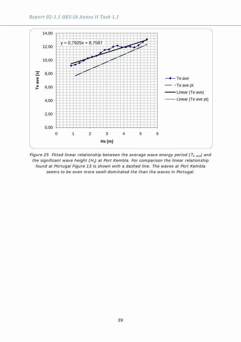
Figure 25 Fitted linear relationship between the average wave energy period (Te ave) and the significant wave height (Hs) at Port Kembla. For comparison the linear relationship

found at Portugal Figure 13 is shown with a dashed line. The waves at Port Kembla seems to be even more swell-dominated the than the waves in Portugal.

y = 0,7925x + 8,7587

0,00

2,00

4,00

6,00

8,00

10,00

12,00

14,00

0 1 2 3 4 5 6

Te a

ve [s

]

Hs [m]

Te ave

Te ave pt

Linear (Te ave)

Linear (Te ave pt)


40

7 Bibliography

1. Nielsen, K. Development of recomended practices for testing and evaluating oceanenergy systems. s.l. : IEA-OES, 2003. 2. Pierson W.J., Moskowitz L. A proposed Spectral Form for fully developed seas Based on the Similarity Theory of S.A Kitaigorodskii. s.l. : J. of Ggeophysical Research, vol 69 no 24 Dec 1964, 1964. 3. Pontes, M.T. Assessing the European Wave Energy Resource. s.l. : Journal of Offshore Mechanics and Arctic Engineering, vol 120, P226-231, 1998. 4. M.F.Burger, P.H.A.J.M. Van Gelder,F.Gardner. Wave Energy Converter Performance Stardard "A Commercial tool". s.l. : EWTEC, 2006. 5. K. Nielsen Ramboll, M. Rubjerg DHI, M. Hesselberg DMI. Wave Atlas for the Danish part of the North Sea. 1999. 6. The Met Office, Proudman Oceanographic Laboratory. Atlas of UK Marine Renewable Energy Resources. s.l. : Beer, 2008. 7. Williams, Martin O. Wave mapping in UK waters, RESEARCH REPORT 392. 2005. 8. K.Nielsen; T.Lewis. Testsite questionaire. s.l. : IA-OES, 2009. 9. www.awsocean.com/archimedes_waveswing.aspx. [Online] AWS Ocean Energy Ltd. 10. www.pelamiswave.com/. [Online] Pelamis Wave Power Ltd, 2010 йил. 11. www.aw-energy.com. [Online] AW Energy. 12. Nielsen, K. Hanstholm phase 2B, Offshore Wave Energy Test. s.l. : Danish Wave Power Aps, November 1996. 13. www.wavestarenergy.com. [Online] Wave Star A/S, 2010 йил. 14. www.danwec.com. [Online] DANWEC. 15. K. Nielsen, N. I. Meyer. The Danish Wa Energy Programme, Second Year Status. s.l. : Proceedings of the fourth European Wave Energy Conference, 2000. 16. www.ecofys.com/com/news/pressreleases2002/pressrelease02aug2002.htm. [Online] 17. Nielsen, K. Pointabsorber survival testing. s.l. : RAMBOLL, 2000. 18. www.wavedragon.net/. [Online] Wave Dragon Aps, 2010 йил. 19. P. Frigaard P, T. L. Andersen. Effektmålinger på Wave Star i Nissum Bredning. s.l. : Aalborg Universitet, 2009. 20. www.folkecenter.dk/da/wave-test-site/wave-test-site.htm. [Online] 2010 йил. 21. P.Frigaard P, J.P. Kofoed. Determination of hydraulic responce of the wave energy converter Wave Dragon. s.l. : Dept. of Civil Engineering, Aalborg University, 2004. 22. Alvarez, Aina Figueras. Estimation of available wave power in the near shore area around Hanstholm harbour. s.l. : Aalborg University, 2010. 23. Stephen, Salter. http://www.mech.ed.ac.uk/research/wavepower/. [Online] 24. www.wavegen.co.uk/index.html. [Online] Wavegen, 2010 йил. 25. www.aquamarinepower.com. [Online] 26. www.emec.org.uk. [Online] 2010 йил. 27. Marine Energy Test Center, Stromness, Orkney. s.l. : Highlands & Islands Enterprise, November 2001. report EX 4471. 28. Kenny, JP. SW Wave Hub Metocean Design Basis. April 2009. 29. The wavepower climate at the Wave Hub site. Aplied Wave Reseach. s.l. : South West Regional Development Agency, November 2006. 30. Wave Hub Development and Design Phase, Wave Energy Converters Mooring System Study. May 2006. 31. www.wavebob.com/. [Online] Wavebob, 2010 йил. 32. www.oceanenergy.ie. [Online] OceanEnergy, 2010 йил. 33. www.marine.ie . [Online] 34. www.oceanlinx.com. [Online] 2010 йил.

annex ii task 1.1 generic and site-related wave energy data

Documents