anl-et/02-23 development of comprehensive models
TRANSCRIPT

ARGONNE NATIONAL LABORATORY
9700 South Cass Avenue, Argonne Illinois 60439
ANL-ET/02-23
DEVELOPMENT OF COMPREHENSIVE MODELS FOR OPACITIES AND RADIATION TRANSPORT FOR
IFE SYSTEMS
By
V. Tolkach, V. Morozov, and A. Hassanein
Energy Technology Division
July 2002

Argonne National Laboratory, a U.S. Department of Energy Office of Science laboratory, is operated by The University of Chicago under contract W-31-109-Eng-38.
DISCLAIMER This report was prepared as an account of work sponsored by an agency of the United States Government. Neither the United States Government nor any agency thereof, nor The University of Chicago, nor any of their employees or officers, makes any warranty, express or implied, or assumes any legal liability or responsibility for the accuracy, completeness, or usefulness of any information, apparatus, product, or process disclosed, or represents that its use would not infringe privately owned rights. Reference herein to any specific commercial product, process, or service by trade name, trademark, manufacturer, or otherwise, does not necessarily constitute or imply its endorsement, recommendation, or favoring by the United States Government or any agency thereof. The views and opinions of document authors expressed herein do not necessarily state or reflect those of the United States Government or any agency thereof.
Available electronically at http://www.doe.gov/bridge Available for a processing fee to U.S. Department of Energy and its contractors, in paper, from: U.S. Department of Energy Office of Scientific and Technical Information P.O. Box 62 Oak Ridge, TN 37831-0062 phone: (865) 576-8401 fax: (865) 576-5728 email: [email protected]


ii
CONTENTS ABSTRACT.....................................................................................................................................1 1. INTRODUCTION .......................................................................................................................1 2. BASE MODELS FOR LOW-Z PLASMA..................................................................................3
2.1. Calculation of Energy Level Structure of Atoms and Ions.................................................5 2.2. Calculation of Transition Probabilities ...............................................................................7 2.3. Collisional-Radiation Equilibrium Model ..........................................................................8 2.4. Opacities ...........................................................................................................................11 2.5. Broadening of Spectral Lines............................................................................................13 2.6. Accounting for Effects Enhancing the CRE Model..........................................................15
2.6.1. Escape Probability Approximation..........................................................................15 2.6.2. Photoionization Process ...........................................................................................15 2.6.3. Auger Process ..........................................................................................................16
2.7. Nonsteady State Approximation .......................................................................................18 3. MODEL OF OPACITIES FOR HIGH-Z PLASMA.................................................................19
3.1. Theory of Electrostatic and Spin-Orbit Splitting ..............................................................20 3.2. Numerical Calculation of Angular Functions fk, ak, bk .....................................................23 3.3. Calculation of Spin-Orbit Splitting...................................................................................24 3.4. Relative Intensities and Transition Probabilities in Lined Spectrum................................26 3.5. Ion Balance and Populations of Levels.............................................................................27
4. RADIATION TRANSFER MODEL.........................................................................................29 4.1. Method of Inward/Outward Directions.............................................................................30 4.2. Approximation of Multigroup Opacities ..........................................................................33 4.3. Radiation Transport in Continuum Spectrum...................................................................34 4.4. Radiation Transport in Lined Spectrum............................................................................35 4.5. Three Modes of Opacity Calculations ..............................................................................36
5. NUMERICAL RESULTS .........................................................................................................36 5.1. ICF Reactor Design Concept ............................................................................................37 5.2. Opacities at Given Pressure ..............................................................................................38 5.3. Preliminary Calculations of Hydrodynamic Processes.....................................................39 5.4. Significance of Line Radiation Transfer...........................................................................41 5.5. Numerical Simulation in Self-Consistent Non-steady State Model .................................44 5.6. Importance of Electrostatic and Spin-Orbit Splitting .......................................................47 5.7. Radiation Flux into Wall for Various Initial Pressure Values ..........................................51
6. SUMMARY...............................................................................................................................55 ACKNOWLEDGMENTS .............................................................................................................56 REFERENCES ..............................................................................................................................57

iii
FIGURES Fig. 1: Radiation to inner zone.................................................................................................32 Fig. 2: Radiation in proper zone ..............................................................................................32 Fig. 3: Radiation to outer zone.................................................................................................33 Fig. 4: Typical ranges of absorption coefficient ......................................................................39 Fig. 5: Hydrodynamics and radiation transport in continuum .................................................40 Fig. 6: Amount of energy at chamber wall for 0.05 torr Xe....................................................42 Fig. 7: Spectral distribution of radiation flux at chamber wall ................................................43 Fig. 8: Fragments of spectral intervals of radiation flux at the wall ........................................43 Fig. 9: Spatial distribution of radiation flux in two models.....................................................44 Fig. 10: Spatial distribution of secondary radiation at 100 sµ ................................................45 Fig. 11: Spatial distributions of temperature and average charge............................................46 Fig. 12: Radiation flux at 20 ns................................................................................................48 Fig. 13: Percentage of prim/sec over gas absorbed energy at the wall ....................................48 Fig. 14: Absorption coefficient of Xe plasma at 50 eV............................................................49 Fig. 15: Absorption coefficient of Xe plasma at 500 eV..........................................................50 Fig. 16: Spatial distribution of radiation flux in three models.................................................51 Fig. 17: Total prim/second radiation fluxes at chamber wall for 0.05 torr Xe........................52 Fig. 18: X-ray spectrum at the chamber wall...........................................................................53 Fig. 19: Radiation flux at the wall by line splitting model ......................................................53 Fig. 20: Amount of initial fluxes arriving to the chamber wall as function of pressure..........54

1
ABSTRACT
An ignition in an inertial confinement fusion (ICF) reactor results in X-ray spectra and ion fluxes moving toward the chamber wall with different velocities. During flight, parts of the energy will be deposited either in the residual and/or protective chamber gas or in the initial vapor cloud developed near the wall surface from vaporization. The deposited energy will be re-radiated to the chamber wall long after the ignition process. The exact amount of energy deposited/radiated and time of deposition are key issues in evaluating the chamber response and the economical feasibility of an ICF reactor.
The radiation processes in the protective gas layer or in the vapor cloud developed above the first wall play an important role in the overall dynamics of the ICF chamber. A self-consistent field method has been developed to calculate ionization potentials, atom and ion energy levels, transition probabilities, and other atomic properties used to calculate thermodynamic and optical characteristics of the plasma by means of collisional-radiation equilibrium (CRE). The methodology of solving radiation transport equations in spherical geometry and the dependence of results on the chosen theoretical model are demonstrated using the method of inward/outward directions.
1. INTRODUCTION
The chamber walls in inertial confinement fusion (ICF) reactors are exposed to harsh conditions following each target implosion. Key issues of the cyclic operation include intense photon and ion deposition, wall thermal and hydrodynamic evolution, wall erosion and fatigue lifetime, and chamber clearing and evacuation to ensure desirable conditions prior to the next target implosion. Several methods for wall protection have been proposed in the past, each having advantages and disadvantages. These methods include use of solid bare walls, gas-filled cavities, and liquid walls/jets. Detailed models have been developed for reflected laser light, emitted photons, and target debris deposition and interaction with chamber components. These models have been implemented in the comprehensive HEIGHTS software package.
The intense power to the first wall resulting from X-rays, neutrons, energetic particles, and photon radiation is high enough to damage and dynamically affect the ability to reestablish chamber conditions prior to the next target implosion. In the case of a dry-wall protection scheme, the resulting target debris will interact with the surface wall materials in different ways. This can result in the emission of atomic (vaporization) and macroscopic particles (i.e., liquid droplets or carbon flakes), thereby limiting the lifetime of the wall. The mass loss in the form of macroscopic particles can be much larger than the mass loss due to surface vaporization and has not been properly considered in past studies as part of the overall cavity response and re-establishment. These processes could seriously affect the power requirements and the economic feasibility of an ICF reactor.
The overall objective of this work is to create a fully integrated model within the HEIGHTS software package [1] to study chamber dynamic behavior after target implosion. The model includes cavity gas hydrodynamics, the particle/radiation interaction, the effects of various heat sources (e.g., direct particle and debris deposition, gas conduction, convection, and

2
photon radiation), chamber wall response and lifetime, and the cavity clearing. The model emphasizes the relatively long-time phenomena following the target implosion up to the chamber clearing in preparation for the next target injection. It takes into account both micro- and macroscopic particles (mechanisms of generation, dynamics, vaporization, condensation, and deposition due to various heat sources: the direct laser/particle beam, debris and target conduction, convection, and radiation). These processes are detrimental and of importance to the success of inertial fusion energy (IFE) devices [2].
The hydrodynamic response of gas-filled cavities has also been calculated in detail by means of new and advanced numerical techniques [3]. In addition, fragmentation models of liquid jets as a result of the deposited energy have also been developed, and the impact on chamber clearing dynamics has been evaluated [4].
The focus of this study is to critically assess the gas protection method by studying the impact of changing chamber gas parameters such as temperature, pressure, and density. For these varying conditions, we determined radiation flux in the chamber as a function of initial gas pressure. We also estimated the dependence of the secondary plasma radiation to the chamber wall, as well as the time- and frequency-dependent radiation properties as a function of the power of the ignition and initial pressure in the chamber. The goal of the report is to demonstrate the dependence and sensitivity of plasma characteristics on the chosen atomic and plasma models. Theoretical analysis of physical processes inside the chamber is essential in choosing adequate physical models and in performing accurate numerical simulation [5, 6].
The Hartree-Fock-Slater (HFS) and Hartree-Fock (HF) self-consistent field methods are both used in this report to calculate atomic quantum behavior. The exchange potential of the HFS method is used in statistical form, while spin-orbit level splitting for non-filled shells is neglected. From the numerical implementation standpoint, the HFS method is easier and significantly more stable than the pure HF method. The HFS equations are solved by an iterative method, yielding wavefunctions, ionization potentials, and energy levels. These values are used to calculate oscillator strengths of discrete transitions, photo-ionization cross-sections, line broadening constants, and other atomic data.
Based upon the obtained atomic data, the collisional-radiation equilibrium model (CRE) is used to calculate the ion population balance of the plasma, thermodynamic functions, and the coefficients of absorption and emission. Ion balance of plasma and populations of atomic levels are determined from detailed analysis of collisional and radiative atomic processes. Collisional processes include collisional excitation and re-excitation, collisional ionization, and three-body recombination. Radiative processes include discrete spontaneous transitions, photo-recombination, and dielectronic recombination.
In calculating the structures of energy levels and ionization potentials for low-Z elements, we employed the non-relativistic approximation of HFS [7, 8 9]. In this approximation, electrostatic and spin-orbit splitting of energy levels are usually neglected. In calculating energy level structures of intermediate- and high-Z elements, the situation is more complicated, because relativistic effects become noticeable, and the electrostatic and spin-orbit splitting is comparable to the ionization potential. The use of HF with full self-consistency is complicated because the self-consistent calculations need to be done separately for each term J
SL , where S, L, J are the

3
corresponding spin-, orbit-, and total momenta of the shell. The implementation of this procedure is especially difficult for non-filled d and f shells.
In this report, we propose a method of calculation for electrostatic and spin-orbit splitting of non-filled p, d, and f shells. The method is based upon perturbation theory using HFS wavefunctions. This method allows calculation of energy level splitting and wavelength, as well as relative strength of spectral lines for ions which have up to three non-filled shells. If the energy level splitting is comparable to the energy transitions between levels, the former may influence the rates of collisional and radiative transitions. Such effects are taken into account by the CRE model extended for high-Z elements.
The processes of radiative excitation and photoionization are neglected in the CRE model [10]. Detailed analysis of the processes of radiative excitation is possible by combined resolution of the equations of atomic-level kinetics and radiation transport in the whole plasma volume, so that the solution is self-consistent for radiation. In such a case, the problem becomes nonlocal, and its implementation requires significant computational resources. In this report, we consider the self-consistent effects in simplified form of the escape factor for line transitions and direct photoionization for the continuum spectrum.
The structure of internal energy levels for high-Z elements is greatly different from the structure of levels for low-Z elements [11]. In photoionization of an electron from the inner shell of a high-Z element, the energy of an appearing vacancy may appreciably exceed the ionization potential. In this case, Auger processes, or processes of ionization without radiation, may take place. At electron photoionization from the inner shell, the effective ionization degree may exceed one. Our proposed model accounts for these processes.
The micro-target ignition in a chamber runs for a very short time, approximately 10-20 ns. In this case, the characteristic time of changing macro parameters in the plasma becomes comparable to that of the micro processes, and the steady-state approximation of the CRE model may become inaccurate. Usually, this simulation reveals inconsistencies in the plasma ionization degree and local values of temperature and density at a given period. Such possible effects were also taken into account by including the non-steady state case in our model.
The calculations are carried out by a computer code developed by the authors, which is now part of the HEIGHTS package [1]. Section 2 describes the major mathematical models used in calculating the atomic and optical characteristics for low-Z elements. An extension of the model to high-Z elements is discussed in Section 3. Section 4 presents a modified method involving inward/outward directions to resolve the radiation transport equation in 1-D spherical geometry. Considering several variants of a micro-target ignition in a chamber, we demonstrate in Section 5 the consequences of accounting for, or neglecting, particular processes in the simulation of dynamic progress for plasma macro parameters and the total characteristics of the plasma radiation fluxes to the chamber wall. Section 6 summarizes the obtained results.
2. BASE MODELS FOR LOW-Z PLASMA
Plasma dynamic problems are usually complex in their initial statement and consist of several independent but interconnected parts. They generally involve calculation of hydrodynamics, radiation transport in the plasma, equations of state, and opacities, dependent

4
upon hydrodynamic macro parameters. Either hydrodynamics or radiation transport can be the most important part, depending upon the physical conditions and plasma state.
Hydrodynamic equations are traditionally written in terms of pressure and internal energy (or enthalpy), whereas the equations of radiation transport are in terms of temperature and density. The hydrodynamic and radiation transport equations are generally resolved self-consistently, because the solution of the radiation transport equations involves the redistribution of internal energy by means of radiation processes in the plasma. The equations of state establish a unique correspondence between parameters used in hydrodynamics and parameters used in radiation transport. They play a part as a connecting link between hydrodynamic and radiation transport parameters. However, these equations also use additional information on the ionic and electronic concentrations in the plasma, which, in turn, depend on the charge distribution in the plasma and populations of atomic levels.
In the radiation transport equations, the optic coefficients of absorption and emission are used. These coefficients correspondingly define the portion of absorbed or emitted energy in the hydrodynamic zone. Opacities not only depend upon temperature and density of the plasma, but also on complicated non-monotonic functions regarding the frequency of absorbed or emitted radiation. Experimental data for these values are incomplete, available for a limited number of elements, and given in restricted ranges. Numerical computation of opacities by means of simplified models leads to unsatisfactory results, but in practice, the use of highly accurate methods results in complex and intricate theoretical solutions and intensive computations. In general, it is assumed that the processes of absorption and emission in the plasma are defined by populations of levels and cross-sections of various atomic processes.
The calculation of populations of atomic levels and ion structure of the plasma is essential for the complete solution of the whole problem. The diversity of methods to find these characteristics is determined by the type of assumptions made, by accounting for or neglecting different atomic processes, and by the modes of numerical implementation.
The major computational models described in this section use atomic parameters calculated by means of such self-consistent field methods as HF and HFS approximations. The calculated values for energy levels, radial wavefunctions, and oscillator strengths are later used to calculate other energetic and probabilistic characteristics, such as the probabilities of spontaneous transitions, the photoionization cross-sections, and the constants of radiation broadening of spectral lines. Our method using the balance condition for collision and radiation processes, will calculate the populations of atomic levels with help from the CRE model approximation; the limits of its applicability are discussed in this section. The situations that are studied exceed the constraints of the CRE model approximation, and methods are suggested to extend the model. We suggest that the CRE model account for photoionization and photoexcitation processes in the form of the escape factor for spectral lines, and direct photoionization from ground and inner states. The photoionization from deep inner states may generate cascades of Auger processes. Special attention is paid to the calculation of populations of atomic levels in the non-steady state approximation. Its applicability is essential in description of fast processes.
The HFS and CRE models were repeatedly tested for several individual elements and mixtures, and appropriate results were calculated for the atomic and plasma characteristics of
5
low-Z elements [12, 13]. In calculation of the atomic and plasma characteristics for high-Z materials, one must take into account the complex structure of their atomic levels [14]. We shall show in this report that appropriately modified models yield satisfactory results for high-Z elements.
2.1. Calculation of Energy Level Structure of Atoms and Ions
Atomic properties are normally calculated by means of quantum mechanics. For example, the wavefunction of a many-electron atom is found from resolution of the Schrödinger equation. In its general state, this equation is quite difficult to resolve. Several methods are in use to simplify the problem. These methods account first of all for symmetry of a quantum system, different forms of the equation itself, and the representation of a wavefunction in some fashion. We will not discuss several well-known methods, such as the method of effective charge of a nucleus, and the Thomas-Fermi method, because their results are very approximate and inaccurate [15]. To describe a spherically symmetrical quantum system, the self-consistent field method is believed to be the most effective, and the HF method is one of the most accurate [16, 17]. However, for our purposes the HF method is not stable enough and quite complicated to implement. The HFS method is a simplification of the HF method. Despite insignificant deterioration in the accuracy, this method is very convenient for numerical implementation because of its stability [7, 8]. The HFS method allows one to implement modified realizations, which remarkably improve the quality of the obtained atomic information. The basis of the numerical calculation of the major atomic properties of a many-electron atom in our study is a combination of HF and HFS methods.
In the condition of central symmetry, a wavefunction of an N-electron atom can be represented in the form of the product of radial and angular constituents
),,,( 21 Nrrr rK
rrΨ ),,,( 21 NrrrR K= ),,,( 2211 NNY ϕθϕθϕθ K× . The methods for calculating angular wavefunction Y are defined by the theory of angular momenta and discussed in Section 3. Further simplifications of the radial wavefunction R are defined by the type of approximation. In the HFS method the potential of direct electron interaction is calculated from the radial wavefunction of participating electrons, and exchanged interactions are averaged in the form of exchanged potential. The radial wavefunction of an atom can be presented as the product of radial wavefunctions of the electrons: ),,,( 21 NrrrR K )()()( 21 2211 Nlnlnln rPrPrP
NN××= K . It is
assumed that equivalent electrons have the same wavefunction.
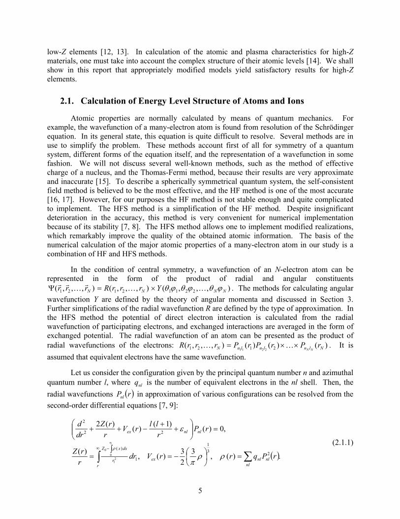
Let us consider the configuration given by the principal quantum number n and azimuthal quantum number l, where nlq is the number of equivalent electrons in the nl shell. Then, the radial wavefunctions ( )rPnl in approximation of various configurations can be resolved from the second-order differential equations [7, 9]:
( ).)(,323)(,)(
,0)()1()()(2
231
1
)(
22
2
21
1
00
∑∫ =
−=
∫=
=
+
+−++
∞ −
nlnlnlex
rr
dxxZ
nlnlex
rPqrrVdrrrZ
rPrllrV
rrZ
drd
r
ρρπ
ε
ρ (2.1.1)

6
Traditionally, in atomic physics, the energies are expressed in Rydberg, 1Ry = 13.6 eV, and distances are in 0a or Bohr units, ma 11
0 1029.5 −×= :
nlε − binding energy of the electron, Ry,
)(rZ − effective charge of the ion field,
)(rVex − potential of exchanged interactions, Ry,
0Z − the charge of the nucleus,
)(rρ − the electron density, Bohr units.
The following normalization condition is applied for radial wavefunctions:
∫∞
=0
2 1)( drrPnl . (2.1.2)
Numerical resolution of Eq. (2.1.1) is performed by an iterative Newton-Raphson-like method. As an initial guess, a hydrogen-like wavefunction 0
nlP was chosen. At iteration i, improved solution i
nlP was obtained from the previous iteration 1−inlP [9]:
inl
inl
inl PPP )1(1 αα −+= − , (2.1.3)
where α is a defining coefficient of the method. Herman and Skillman [9] suggest α between 0.3 and 1. Strictly speaking, ),( inlαα = is a vector and depends upon both configuration nl and iteration number i. However, the convergence of HFS equations is smooth enough, and α may be taken as 0.5 for all configurations and iterative steps without significant increase in the number of iterations.
In the numerical procedure involving Eq. (2.1.1), the eigenvalues nlε and eigen-wavefunctions )(rPnl are found, from which the distribution of the charge in the atom ( )rZ and exchanged potential ( )rVex are calculated. The solution is considered to be calculated when all
eigenvalues converge to δεεε ≤− − inl
inl
inl
1 , where the parameter δ is chosen to be small enough. Koopman’s theorem implies that the binding energy of the electron in the atom is equal to the eigenvalue [18]. From )(rZ and )(rVex , the binding energies and wavefunctions of excited states, and the wavefunctions of the continuum spectrum for given energy E of free electron are derived. The calculation of the wavefunctions for the continuum spectrum has its own specifics, because these functions are normalized to a δ function:
)()()(0
llEEdrPrP lEEl ′−′−=′′
∞
∫ δδ . (2.1.4)

7
The set of binding energies nlε for maxnn ≤ forms the structure of the energy levels, and each value represents the energy required to remove a given electron from the atom. Because the value of the binding energy of an excited electron is inversely proportional to 2n , the choice
10max =n provides that 99% of a discrete spectrum is taken into account.
2.2. Calculation of Transition Probabilities
The wavefunctions found from resolution of the HFS equations can be used to calculate energetic and probabilistic ion properties. The wavelengths and spin-orbit splitting constants are the main energetic properties. The probabilistic properties, such as oscillator strengths and photoionization cross-sections, are expressed through the matrix elements of two or more radial wavefunctions of participating initial and final states.
In approximation of the one-electron atom, or in the case of the only electron above the filled shell, the oscillator strength ( )11, lnnlf of a transition from one state, given by the set of quantum numbers nl with q equivalent electrons, to another state, given by the set of numbers
11ln , is expressed [19]:
( ) ( )2111
11
12,max
32),( ln
nlRl
llmlnnlf+
=−h
ω . (2.2.1)
Standard notation is used here for the electron mass m, the electron charge e, and the Planck constant h . At the transition from one state to another state, the absorbed or emitted photon has frequency ω . The matrix element of the radial wavefunction 11ln
nlR is defined as
∫∞
⋅⋅⋅=0
)()(11
11 drrPrrPR lnnlln
nl , in Bohr units. (2.2.2)
The summation rule is valid for oscillator strengths, i.e., the sum of all oscillator strengths from the given state a to the other states is equal to the number of the electrons in this state:
ab
ab qf =∑ . (2.2.3)
The transitions to the continuum are expressed in terms of photoionization cross-sections ( )ωσ nl , which determine the relative probability of absorption of a photon by the atom, when
radiation is passing through the area:
( ) ( )2
1max
22
1234)( lE
nlll
nl Rlle ′
±=′∑+
=ωπωσ , 2cm . (2.2.4)
To calculate the photoionization cross-sections, dipole transitions are summed to states 1+=′ ll and 1−=′ ll . The energy of passing radiation is equal to ωh . Matrix element lE
nlR ′ is defined by the integral

8
drrPrrPR lEnllE
nl )()(0
′
∞′ ⋅⋅= ∫ . (2.2.5)
The Einstein coefficient abA , which defines the probability of spontaneous transition from level a to level b, is expressed through the oscillator strength [19]
( )ab
baab f
cmEEeA 23
222h
−= , 1−s , (2.2.6)
where c is speed of light, and aE and bE are the binding energies of the electron in the upper and lower states, respectively. The Einstein coefficients are also used later in determining the constants of radiation broadening. In calculating the photoionization cross-sections for a free electron with energy E and wavefunction in the final state )(rElΨ , the wavefunction is also calculated by the HFS method following an additional procedure that accounts for splitting of the absorption threshold. This procedure is discussed in Section 3.4.
2.3. Collisional-Radiation Equilibrium Model
The ionization structure of the plasma and populations of atomic levels are generally found from the system of non-steady kinetic equations, which can be written
jiji
jij
ijii KNKN
dtdN ∑∑
≠≠
+−= , 13 −scm . (2.3.1)
The population iN of atomic level i is determined by the set of transitions from this level to other levels j with transition rates ijK , as well as transitions from other levels j to this level i with transition rates jiK . One equation is written for each atomic level. If level i defines the ground state, then the population of this atomic level gives the concentration of the ion in the plasma.
Electronic transition rates depend on such macro parameters of the plasma as temperature and density. If one assumes that the atomic transition processes are significantly faster than typical thermodynamic processes of the plasma, then the atomic system is in an equilibrium state at each hydrodynamic time step. This observation means that the populations of atomic levels do not depend on time, and Eq. (2.3.1) can be transformed to a system of equations in a steady-state approximation. This system is written in the form of homogeneous algebraic equations:
0=+− ∑∑≠≠
jiji
jij
iji KNKN , 0=dt
dNi . (2.3.2)
In addition to the kinetic equations, Eqs. (2.3.1) and (2.3.2) have to contain the frequency-dependent equations of radiation transport, because the kinetic rates of radiation excitation and photoionization depend on the radiation flux. The problem is spatially non-local and defined by the radiation processes in the whole plasma domain. In some cases, the processes of photoexcitation are used to account for local formulation by means of the so-called escape
9
factor approximation [20, 21]. However, this approximation is not universally applicable but restricted to several conditions.
The CRE approximation accounts for collisional processes, as well the processes of photo de-excitation and photorecombination. It neglects the processes of photoexcitation and photoionization. Remaining local, the CRE model satisfactorily describes the state of an optically thin plasma in wide ranges of temperature and density. Further simplifications of the CRE model leads to important particular cases, which narrow the limits of model applicability. Neglecting all radiation processes, for example, results in an approximation of the local thermodynamic equilibrium (LTE), which is very often used in the simulation of a low-temperature dense plasma. Another limiting case is the coronal model. Excited states in the coronal approximation are connected only with the ground state. As a consequence, only collisional excitation and radiation de-excitation are considered. Such effects are typical for a very hot, optically thick plasma. Because the CRE model includes all effects mentioned for the limiting cases of LTE and coronal approximations, we considered it as a major model. Later on, this model becomes more complicated as the situation demands.
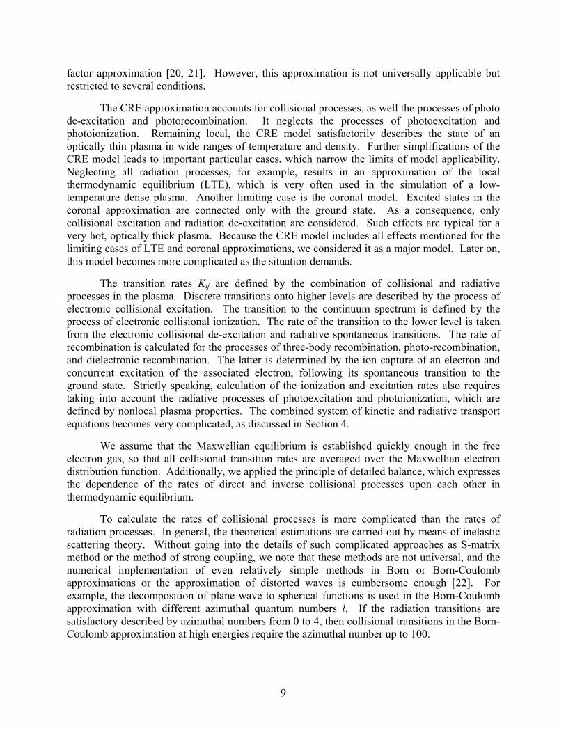
The transition rates Kij are defined by the combination of collisional and radiative processes in the plasma. Discrete transitions onto higher levels are described by the process of electronic collisional excitation. The transition to the continuum spectrum is defined by the process of electronic collisional ionization. The rate of the transition to the lower level is taken from the electronic collisional de-excitation and radiative spontaneous transitions. The rate of recombination is calculated for the processes of three-body recombination, photo-recombination, and dielectronic recombination. The latter is determined by the ion capture of an electron and concurrent excitation of the associated electron, following its spontaneous transition to the ground state. Strictly speaking, calculation of the ionization and excitation rates also requires taking into account the radiative processes of photoexcitation and photoionization, which are defined by nonlocal plasma properties. The combined system of kinetic and radiative transport equations becomes very complicated, as discussed in Section 4.
We assume that the Maxwellian equilibrium is established quickly enough in the free electron gas, so that all collisional transition rates are averaged over the Maxwellian electron distribution function. Additionally, we applied the principle of detailed balance, which expresses the dependence of the rates of direct and inverse collisional processes upon each other in thermodynamic equilibrium.
To calculate the rates of collisional processes is more complicated than the rates of radiation processes. In general, the theoretical estimations are carried out by means of inelastic scattering theory. Without going into the details of such complicated approaches as S-matrix method or the method of strong coupling, we note that these methods are not universal, and the numerical implementation of even relatively simple methods in Born or Born-Coulomb approximations or the approximation of distorted waves is cumbersome enough [22]. For example, the decomposition of plane wave to spherical functions is used in the Born-Coulomb approximation with different azimuthal quantum numbers l. If the radiation transitions are satisfactory described by azimuthal numbers from 0 to 4, then collisional transitions in the Born-Coulomb approximation at high energies require the azimuthal number up to 100.

10
Despite the many theoretical studies to express the cross-section for both collisional and radiative processes, semi-empirical formulas are practically more suitable for numerical estimation of cross-sections of collisional excitation ijσ in transition from level i to level j with oscillator strength of the transition fij and the energy of the transition ijE∆ . In various applications, modifications of the Bethe formula [23, 24, 25] are often used. These modifications do not practically differ from each other. This study utilizes the modification of the Van Regemorter formula [10, 26], which is appropriate to obtain the rate ijvσ of the collision dipole transition of electrons:
).(2
3)(,
,),()exp(102.3 13212
3
7
βπ
ββ
βββσ
−≈∆
=
−
∆⋅×= −−
EipTE
scmpE
Ryfv
ij
ijijij
(2.3.3)
In the expression above, the function ( )β−Ei is known as the exponential integral, and T is the temperature of the plasma.
The rate of the inverse process of collisional electronic de-excitation is defined from the detailed balance condition:
jjiiij NvNv σσ = , 1−s . (2.3.4)
To estimate the rate of the collisional electronic ionization, Lotz [27] has suggested the universal formula with number of equivalent electrons in the shell q and ionization potential of an ion I:
( ) ( ) ( ).exp,
,),(106 1321
23
8
βββββ
ββσ
−−==
⋅
⋅×= −−−
EifTI
scmfI
Ryqv i (2.3.5)
In the case of ionization, accounting for detailed balance conditions gives the rate coefficient rvv σ21 of three-body recombination [10]:
( ) ,,exp22
1623
2
121
−
+
= scmv
mTggvv i
z
zr σβπσ h (2.3.6)
where zg is the statistical weight of ion z; the other values are defined as above.
The Kramers formula gives a quite good approximation for the rate of photo-recombination ( νχ ) on the hydrogen-like levels [10,19]:

11
( )( ) [ ]
,
,,)()exp(13733
32
2
2
1323
30
TnRyz
scmEizm
ha
n
nnn
=
−⋅−⋅⋅⋅= −
β
βββπ
χν
(2.3.7)
where 0a is the Bohr radius, and z is the spectroscopy symbol.
Dielectronic recombination is a two-electron process. By exciting an atomic electron, a free electron is captured in the upper state of the ion. The exciting electron transits radiation to its initial state. Accounting for the captured electron, the ion charge is decreased by a unit, i.e., the process of recombination has occurred. The rate of dielectronic recombination is comparable to the rate of photorecombination [28] and, therefore, cannot be neglected. Many efforts have been made to improve the accuracy of the dielectronic recombination rate. Some authors pointed out that different approaches still tend to disagree by factors of two or more [29, 30]. For many ions, and Xe is among them, the Burgess formula [28] is the only choice. In notation introduced above, this formula may be written
( ) ( )[ ]( )
( ) ( ).
1,
1015.01,1
,1015.01105.014.13
480
,),exp(10)(
2
1
2
32
1222
1323
13
RyzE
zz
TRyz
zzz
zfB
scmB
ijd
ijd
ddd
+
∆=
++=
+=
⋅+⋅++⋅++
=
−=
−
−
−−
χχχβ
χχχχββακ
(2.3.8)
2.4. Opacities
In accordance with the general scheme of allowed energy states of an atomic system, the electronic transitions and their accompanying absorption and emission of photons are subdivided into three types: bremsstrahlung, photoionization from ground, excited and inner shells, and discrete transitions. The latter is approximated in the form of dipole transitions between ground and excited states, the transitions between excited states, and partly, the transitions from inner shells. Because of their importance, the profiles of spectral lines are processed very carefully by means of all major broadening mechanisms, including radiation, Stark, Doppler, and resonance broadenings [31].
In collision-radiation equilibrium, the total absorption coefficient Ktot depends on local values of temperature T, density ρ , and ionization Z of the plasma. It is usually expressed as a summation of absorption coefficients, containing the contribution for each free-free, bound-free, and bound-bound transition. Each effect is defined by its cross-section. The total absorption coefficient is then given as
Ktot T,ρ,hω( )= K ff T,ρ,hω( )+ Kbf T,ρ,hω( )+ Kbb T,ρ,hω( ), cm -1, (2.4.1)
where
12
K ff (T,ρ,hω) = Ne T,ρ( )× σ i
ff T,hω( )i
∑ 1− e−hω kT( )Ni T,ρ( ), cm−1,
,),,()(),,( 1−⋅= ∑∑ cmTNTK iji j
bfijbf ρωσωρ hh
.),,()(),,( 1−⋅= ∑∑ cmTNTK iji j
bbijbb ρωσωρ hh
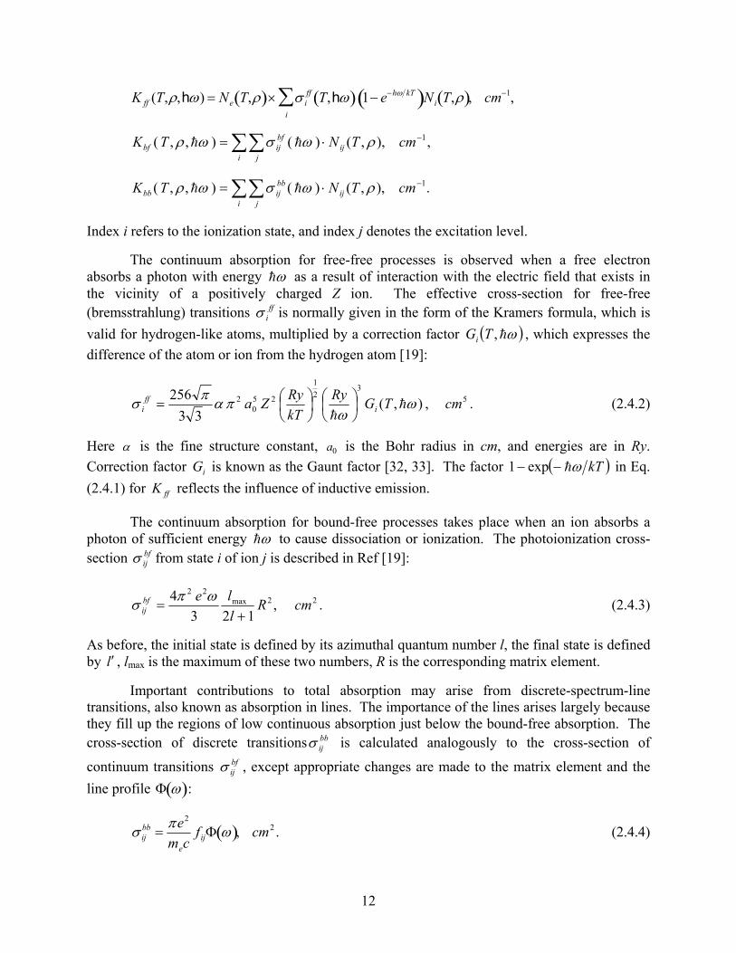
Index i refers to the ionization state, and index j denotes the excitation level.
The continuum absorption for free-free processes is observed when a free electron absorbs a photon with energy ωh as a result of interaction with the electric field that exists in the vicinity of a positively charged Z ion. The effective cross-section for free-free (bremsstrahlung) transitions ff
iσ is normally given in the form of the Kramers formula, which is valid for hydrogen-like atoms, multiplied by a correction factor ( )ωh,TGi , which expresses the difference of the atom or ion from the hydrogen atom [19]:
),(33
256 321
250
2 ωω
παπσ hh
TGRykTRyZa i
ffi
= , 5cm . (2.4.2)
Here α is the fine structure constant, 0a is the Bohr radius in cm, and energies are in Ry. Correction factor iG is known as the Gaunt factor [32, 33]. The factor ( )kTωh−− exp1 in Eq. (2.4.1) for ffK reflects the influence of inductive emission.
The continuum absorption for bound-free processes takes place when an ion absorbs a photon of sufficient energy ωh to cause dissociation or ionization. The photoionization cross-section bf
ijσ from state i of ion j is described in Ref [19]:
,123
4 2max22
Rllebf
ij +=
ωπσ 2cm . (2.4.3)
As before, the initial state is defined by its azimuthal quantum number l, the final state is defined by l ′ , lmax is the maximum of these two numbers, R is the corresponding matrix element.
Important contributions to total absorption may arise from discrete-spectrum-line transitions, also known as absorption in lines. The importance of the lines arises largely because they fill up the regions of low continuous absorption just below the bound-free absorption. The cross-section of discrete transitions bb
ijσ is calculated analogously to the cross-section of
continuum transitions bfijσ , except appropriate changes are made to the matrix element and the
line profile Φ ω( ):
σ ijbb =
πe2
mecfijΦ ω( ), cm2 . (2.4.4)
13
The calculation the line profile is discussed in the next section.
2.5. Broadening of Spectral Lines
Atomic and ionic spectral lines originate from specified electronic transitions between energy levels of atoms and ions, respectively. These transitions are not precisely sharp because of several broadening mechanisms. The result of these mechanisms is that any observed line has a finite width and is described by its profile. Four processes may contribute to the finite width of a spectral line and, consequently, to the line profile: natural broadening, Doppler broadening, Stark broadening, and interaction with neighboring particles.
Natural broadening, or radiation damping, arises from the finite lifetime of an ion in some given state, which leads by the Heisenberg principle to the corresponding energy spectrum. This type of broadening yields the Lorenz profile. Despite the other broadening mechanisms usually being more effective, radiation damping always exists even if there is not any collision, say, in low-density plasmas.
Doppler broadening is due to the thermal motion of the emitting or absorbing atoms. The well-known “Doppler effect” results in shifting the wavelength of moving radiating particles. For a Maxwellian velocity distribution, the Doppler broadened line has a Gaussian profile.
Collisional broadening, or pressure broadening, presents a large problem in spectral modeling and serious complexity in formulating appropriate methodology. Particular mechanisms, which contribute to pressure broadening, are identified with the names of Stark broadening and Holtzmark broadening.
Stark broadening appears at atomic collisions to the charged particles. At each moment, an electron of an atom is subject to a variable outer electric field. Fast changes of the field result in a splitting effect. Consequently, for the level with quantum numbers n, l is split by quantum numbers m and shifted from its unperturbed value. Note also that broadening of hydrogen-like ions is essentially different from the broadening of the other types of the ions, because hydrogen-like ions have l-number degeneracy, which is taken away by the field. The broadening of hydrogen-like ions is thus significantly larger.
It was supposed above that all collisions are paired, and collective effects are negligible. For high densities under the influence of the long-range interaction potential, it is not easy to separate paired collisions from collective collisions. Holzmark broadening is considered as a limiting case, when collective collisions are dominant. The atom is considered to be subject to a fluctuating micro-field generated by the other particles. The fluctuations of atomic levels result in the broadening effect. Holzmark broadening is mostly considered important for hydrogen-like ions, because for the ions of other types, atomic fields may be considered as short-range fields, and collective effects can be described by means of paired effects.
In a low-temperature plasma, the most-mentioned broadening mechanisms may be ineffective. Collisional broadening is negligible at temperatures lower than 1 eV, because the plasma is represented by neutral atoms, and the electronic density is very low. Doppler broadening at low temperature is also very small. Transition rates in neutral atoms are high

14
enough, and this lowers the radiation width. However, if an atom is in an excited state, it can non-radiatively transmit its excitement to the neutral atom by the collision. Reducing the lifetime of the atom in the excited state broadens the level; this effect produces resonant broadening. Denoting statistical weights of upper i and lower j levels as gi and gj, the width of the resonance line width is given as [19]:
ji
jij
ijrez N
gg
fEm
e∆
=∆2
ω , 1−s , (2.5.1)
where Nj is the population of the lower level.
In highly ionized and moderately dense plasmas, Stark broadening dominates all major broadening mechanisms. The energy levels within single atoms may be modified due to the electric field of nearby atoms and ions. This effect is known as the Stark effect, which becomes more pronounced when the density of the plasma becomes greater. Denoting the distance to the nearest level as iE∆ for level i, the Stark line width under binary collisions has a Lorenz profile and may be expressed by the Griem formula [31]:
∆+
∆
=∆
jieS E
kTGjarj
EkTGi
ariN
kTRy
mah
23
23
38 2
0
2
20
202
3
πω , s –1. (2.5.2)
Here, the matrix element is evaluated by using the HFS radial wavefunction ( )rPi :
drrPrrPiari ii )()( 2
020
2
∫∞
= . (2.5.3)
The Griem formula describes inelastic electron broadening, while the collisional Gaunt factor G effectively accounts for the elastic part of the broadening.
To calculate the line profile Φ ω( ), we utilize all broadening mechanisms. For the case of a moderately ionized plasma, it is quite difficult to strictly separate the mechanisms from one another. All broadenings are calculated in the neighborhood of the line center. Natural and Stark broadenings are composed together as they both have a Lorenz profile. Other mechanisms have different profiles, and the correct profile would be the result of convolution of all three profiles, which is a numerically complicated procedure. Instead, we substitute for the two-profile convolution, accounting for the most dominant mechanism for each case. For example, the result of the Gaussian profile with line width Gω∆ and Lorenz profile with line width
Lω∆ convolution is a well-known Voigt profile. The formula [19] is given as
Φ(ω) = κ0aπ
e−y 2
dyu − y( )2 + u2∫ , u =
ω −ω0
∆ωG
, a =∆ωL
2∆ωG
, (2.5.4)
where 0κ is the absorption coefficient in the center of the line, given in cm-1.

15
2.6. Accounting for Effects Enhancing the CRE Model
When an external energy source is absent, the above CRE model satisfactorily describes the optically thin steady-state plasma. However, an optically thick plasma or plasma subject to the external energy flux needs to be characterized by the model in a manner self-consistent with radiation. This self-consistent model is nonlocal and, therefore, laborious for practical use.
One of the methods to include self-consistency in description of the populations of atomic levels is expansion of the CRE model by additional effects. The nature and order of the expansion tend to be adequately conditional and depend upon the initial state of the problem in question. The general approach is introducing such additional nonlocal effects as decreasing the probability of spontaneous transitions (usually in the form of an escape probability approximation), including the probability of photoionization and accounting for Auger processes.
2.6.1. Escape Probability Approximation
A high-temperature quasi-isothermal plasma in large volume is transparent in the local statement of the problem. Such a plasma is balanced as a coronal plasma, and a major part of its radiation belongs to lines that allow one to neglect the process of absorption in the continuum spectrum. For some lines, their optical thickness )(ωκτ l= appears to be greater than unity, i.e., the probability that a photon with frequency ω would move distance l and would not be absorbed appeared to be less than unity. This probability depends on the absorption coefficient
( )ωκ in the line profile, linear dimension of plasma l , and, of course, the profile itself Φ = Φ T,ρ,ω( ). In the case of isothermal plasma, nonlocal effects can be successfully reduced to a local statement: absorption of some of the photons is equivalent to decreasing their spontaneous emission. Therefore, in balancing of the process, accounting for absorption leads to substitution of the probability of spontaneous transition ijW by the value ΘijW , where Θ is the escape factor. In spherical geometry domains, the escape factor is defined as [34]:
( ) ( )( ) ωωτω dΦexpΦ20
sphere−=Θ ∫
∞
, (2.6.1)
where l0κτ = is the optical thickness, and 0κ is the absorption coefficient in the center of the line. The Doppler region in the center of the line usually has optical thickness significantly exceeding unity, whereas “Lorentz wings” usually belong to the region with 1<<τ . That is why the escape factor values are usually situated in the interval 10 <Θ< . The escape factor is defined for all the profile types discussed above.
2.6.2. Photoionization Process
The presence of hard X-ray radiation from powerful sources with a nearly Planckian spectrum is essential for the ICF reactor plasma environment. Accordingly, the initially cold plasma is subject to hard X-ray radiation of a given spectrum, the description of which is best given in terms of the spatial distribution of radiative intensity ( )ωhr,rI . The line spectrum of the

16
plasma absorbs only a very little part of the outer radiation because the line width is negligibly small compared with the width of the emitting spectrum. Moreover, the lines are situated in the long wave part of the spectrum. The photoionization from the ground state and inner shells dominates the absorption outer radiation. Because the power of Planckian radiation is proportional to 4T , the process of photoionization is particularly important in description of a plasma with high-temperature gradients and may dominate over other processes in the kinetic equations of the CRE model, especially at initial time steps.
The probability of photoionization is determined by the integral over all frequencies exceeding the electron binding energy 0ω [34]:
ωωσω
ω
ω
drIW ii )(),(
0
∫∞
=h
hr
, (2.6.2)
where )(ωσ i is the photoionization cross-section. The method for calculating the photo-ionization cross-section was discussed in Section 2.4. The iW values appear in the system of kinetic equations (2.3.2) for the CRE model as additional terms describing photoionization as part of the total energy balance.
As mentioned above, the typical energy of the outer radiation significantly exceeds the binding energy of the electrons in ground and excited states. The photoionization cross-section far off the threshold has an asymptotic behavior close to ( )3
0 ωω . However, since the population of excited states is low enough, photoionization from the excited states can be neglected. Therefore, the number of kinetic equations, specific to absorbing radiation, will be considerably lower than the total number of kinetic equations in solving the problem with complete self-consistency. Additionally, note that accounting for photoionization may be important only if an outer powerful plasma source is present; otherwise, photoionization can easily be neglected. The plasma cannot generate radiation that is energetically higher than the ionization potential of its major ion. The main part of the radiation is situated in the region of the ionization potential of the major ion of the plasma, and the photoionization from the inner shells is negligibly small.
2.6.3. Auger Process
The photoionization of an electron from ground or excited states is a paired inverse process, which involves photorecombination to one of those states. The cross-section and the rate of photorecombination can be determined from the detailed balance condition, if the cross-section and the rate of the direct process are known. Photoionization of inner electrons is somewhat different. Besides the photorecombination, there is a concurrent process called autoionization, i.e., nonradiating transition of an upper electron to a lower level with filling of the vacant state and ionization of one or more outer electrons.
The process of nonradiant filling of an inner vacant state with immediate ionization of an outer electron is called the Auger process, which appears to be a special case of autoionization. Inner vacancies may be formed not only as a result of photoionization by means of an outer
17
source, but also by direct ionization of inner shells subject to external hard electron or ion energy fluxes. The study of those processes exceeds the scope of this report.
Typically, high-Z elements have very complicated structures of inner levels, the energy of which may exceed by several orders of magnitude the ionization potential of a neutral atom. For example, the ionization potential of xenon is nearly 10 eV, while the energy of the inner 1s electron is close to 40 keV. The vacant state formed in the 1s level may be filled up from the shell with n = 2. In turn, the vacant state of the n = 2 shell may be filled up from the shell with n = 3, and so on. Consequently, in accounting for the successive filling of the vacancies, one energy quantum may cause an avalanche of ionized electrons. Typical energies of inner electrons significantly exceed those of outer electrons, and one may assume that the autoionization and cascade formation appear “simultaneously” compared to the time scale of outer electron processes. Because of this, one may calculate the probability of autoionization under the assumption of a steady-state approximation, and the processes of photorecombination to the inner vacant state can be neglected.
Consider the processes of autoionization with probability aW and the processes of radiative stabilization with probability radW . The relative proportion of autoionization electrons
( )radaa WWW +/ depends greatly on the principal quantum number n and effective charge Z. The radiative probability is proportional to 4Z , while the autoionization probability is proportional to Z . The latter explains why the importance of autoionization becomes greater with increasing Z material.
The autoionization probability may be found by a method described in Ref. [10]. Assume an electron with state 1α and orbital momentum 1l jumps to the state 0α with orbital momentum 0l . Then,
( ) ( ) ( ) ( ) ( )[ ] 10101010101 ,,,,,, −∑ ′′⋅′′+′⋅= sllnlWQllnlWQRylnWa
χχχχχ αααααα
h,
where probabilities of direct χW ′ and exchange χW ′′ transitions are defined in terms of direct and
exchange integrals dRχ , eR χχ ′′ , and χQ , χQ ′′ , respectively. We do not write out the formulas for the Q-factors because of their awkwardness; the expressions can be found elsewhere [19]. Just note that radial integrals define the value of the Coulomb and exchange interactions of the electrons, while Q-factors are the relative intensities of different transition components. Parameter χ defines the multiplicity of the process.
We did not study different scenarios for the appearance of the vacancies and their stabilization. Accounting for the factor ( )radaa WWW +/ , the average number of ionized electrons was calculated in forming the vacancy in the nl-shell. In this case, a successive cascade is effectively equivalent to the process of many-electron ionization neAA n +→+ +ωh . Note that the CRE model is usually restricted by eAeA nn 21 +⇔+ +++ and ωh+→+ +++ nn AeA 1 processes. The relative contribution of Auger processes increases with growing Z. However, the

18
effective charge of the shell quickly decreases when the principal quantum number n is increased, and the contribution from the Auger processes also decreases.
2.7. Nonsteady State Approximation
The population levels in the CRE model do not depend on time because the model assumes that the atomic processes occur significantly faster than the typical time of changes for temperature and density of a macroscopic system. In such an approximation, the microscopic system always advances to relax. Simple estimations show that, in our particular case, this assumption is wrong.
Sviatoslavsky et al. [35] report that the target emits 22.5 MJ of incident X-ray radiation during 20 ns. The maximal intensity of X-ray radiation corresponds to the energy interval of photons as 0.1-1 keV. The absorption coefficient of such photons in a plasma with density
16108.1 × cm-3 and temperature 0.3 eV is approximately 0.02 cm-1. In our calculations, the radius of the central zone was chosen as 10 cm, and the optical thickness of this zone is τ = 0.02 cm-1 × 10 cm = 0.2. The zone will absorb 18.082.011 =−=− −τe of total radiative energy, or 0.2 MJ ≈
24102.1 × eV, during the first nanosecond. The central zone contains 7.54 × 10¹⁹ atoms, i.e., the average energy of absorption per atom is approximately 10 keV. Using the CRE model, we estimated that such energy corresponds to temperature 235 eV and mean charge 24.
The ionic charge should be changed since Z = 0 to 25 during 1 ns. It is possible to estimate the ionization time for state Z to Z + 1, using the Lotz formula:
,zez
z
vNNNt
σ∆
=∆ s, (2.7.1)
If we assume that the plasma consists of ions with charge Z, then zz NN =∆ and
ze vNt σ1=∆ . Electron concentration would then be equal to 31710 3.4 −×= cmN e . The
transition from state Z = 0 to Z = 1 is defined by the rate 1360 103.1 −− ⋅×≈ scmνσ . In such a
way, the time required to ionize neutral atoms is equal to nst 0018.0≈∆ . Note that the time required to change from state Z = 23 to Z = 24 is nst 30~∆ , because the ionization rate
131123 10 3.7 −− ⋅×≈ scmvσ in this case is noticeably less.
where zN − concentration of ions with charge Z, cm-3,
eN − electron concentration, cm-3,
zvσ − ionization rate, cm-3 s-1,
zN∆ − number of ions, which change the ionization level from Z to Z + 1 during time step t∆ .

19
Our estimations show that the time required ionizing neutral atoms to the state Z = 24 considerably exceed 1 ns. Consequently, the steady-state approximation of the CRE model is unacceptable. In our case, the ionization states and population levels are to be calculated with Eq. (2.3.1), the nonsteady state kinetic equation.
The transition rates ijK include both collisional processes and the processes of photoabsorption, photorecombination, and dielectronic recombination. We assume that free electrons are in thermodynamic equilibrium, in compliance with the Maxwellian distribution. Otherwise, it would be necessary to solve the kinetic Bolzmann equation, which is essentially more complicated than Eq. (2.3.1). Note also that Eq. (2.3.1) is restricted by the following conditions:
Kijh >> Kij
g , hg tt ∆>>∆ , (2.7.2)
where gt∆ and ht∆ are typical times for the kinetic process from ground and excited states, respectively. These conditions may be easily obtained from the general form of the rates of collisional transitions: these rates have the dependence Kij ~ exp(−∆Eij T). For the transition from the ground state, the ratio TEij∆ is much more than one, but for the transition from the excited states, it is less than 1. The characteristic time of a transition from the highly excited state is quite low, 10-11-10-13 s, which is several orders of magnitude less than the typical hydrodynamic time. As a result, it is unnecessary to solve the system of nonsteady state kinetic equations for all levels. One may use a quasi-stationary approximation in which Eq. (2.3.1) is solved only for ground states of the ions. The populations of excited levels are determined further from the system of linear algebraic equations (2.3.2), in which the populations of ground states are yet known.
3. MODEL OF OPACITIES FOR HIGH-Z PLASMA
Resolution of the Schrödinger equation depends, to a great extent, on the nuclear charge of the element in question and the ionization level of the plasma. This resolution is easier for low-Z elements rather than high-Z elements, and simpler models are able to yield an accurate solution. For example, HFS and HF equations describe the ionic structure sufficiently well until Z is less than 20. Starting from Z = 21, the shells have d electrons. As a result, the amount of computation increases while the accuracy decreases. Continuing further, the shells have f electrons, starting from Z = 58, and the computation becomes very complicated. For such elements, the spin-orbit splitting approximation is inappropriate, and accounting for relative corrections is important. Additionally, electronic collapse may become apparent for d and f electrons, and the interaction between configurations grows. Experimental atomic data for high-Z elements are incomplete and less accurate than those of low-Z elements. This situation reduces the possibility that semi-empirical methods will improve the accuracy of calculations [11]. Nevertheless, calculations for high-Z elements must take into account all distinctive features discussed above because the response of radiation transport at the macro level will depend to a greater extent on the accuracy and details of obtained energy levels.

20
Let us repeat the notation introduced in Section 2. Suppose that an atom is not subject to an outer field. The wavefunction of atom Ψ is equal to the product of the radial function R and the angular function Y:
Ψ(r r 1,
r r 2,...,
r r N ) = R(r1,r2,...,rN ) ×Y (θ1ϕ1,θ2ϕ2,K ,θN ϕN ) .
Further simplification of functions R and Y depends on the properties of the chosen models. In this report we use the following models. The radial wavefunctions and energy levels are found by the HFS method, while relativistic corrections, and electrostatic and spin-orbit splitting of energy levels and lines are found by perturbation theory. We also account for the summation of momenta for s, p, d, and (partly) f electrons. Note, that the mathematical apparatus becomes confusing when the azimuthal quantum number grows large enough.
3.1. Theory of Electrostatic and Spin-Orbit Splitting
The terminology and mathematical techniques of atomic physics are very complex. We shall briefly describe some basic concepts to help the reader better understand the further presentation. As mentioned above, an atomic wavefunction may be decomposed into multiplication of radial and angular parts, and these parts are calculated and treated separately. For example, the radial wavefunctions obtained by the HFS approximation are used later to calculate the whole set of other energetic and probabilistic properties, such as relativistic corrections to energy levels; wavelengths of linear transitions; Slater integrals, which define the direct and exchange electronic interactions; oscillator strengths; and photoionization cross-sections. After deriving the radial wavefunctions, one may calculate all these parameters and save them for future use.
The angular wavefunctions are found separately by summation of electron momenta. The arithmetic addition of orbit and spin momenta is not commutative in quantum mechanics, and its result depends on the order of additives in the mathematical expression. Despite there being ( )!2n ways to carry out the summation for n different electrons, directional methods that regulate the summation are used in practice. One may assume that the strongest interaction is the most probable. Thus in calculating the total momentum, the greater values should be added first; then, the smaller values are added to the result, and so on. This method is called the “parentage scheme approximation” [36].
For low-Z elements with Z less than 30, the electrostatic interaction is high while the spin-orbit interaction can be considered negligibly small. In this case, the total orbit momentum L is calculated first as a sum of the electrostatic momenta for all the electrons of the atom. Then, the total spin momentum S is found separately. Finally, the total momentum is determined from J = L + S. For low-Z elements, LS coupling is said to be a better approximation for the total momentum.
With increasing atomic number of an element, the energy of the interaction of electron orbit momentum to its own spin also increases. For elements with atomic numbers nearly 90, these two types of interaction are comparable, and JJ coupling becomes the more appropriate computation scheme. In this case, the total momentum j is initially calculated for each electron as j = l + s; subsequently, all total momenta j are summed.

21
Let us consider some qnl shell given by its corresponding principal quantum number n, azimuthal quantum number l, and number of equivalent electrons q in the shell. The parentage scheme approximation for a group of equivalent electrons is not appropriate because all these electrons have similar energies of interaction, and one cannot choose any preferred summation scheme. In such cases, the linear combination is carried out for all possible summation schemes with weight coefficients called “parentage coefficients”. In general, the square of the parentage coefficient is defined as the probability to form the term with the set of quantum numbers 11SL after removal of electron ls from the term 00SL . The greater the value of l, the larger the number of possible variants that may occur for the values LS. When two groups of equivalent electrons are considered, the total momentum is calculated by means of the parentage approximation scheme.
Racah [37,38] has presented a detailed analysis of the calculation of parentage coefficients and classification of groups of equivalent electrons. This methodology is widely used and now called the Racah technique.
As mentioned above, the summation of momentum in quantum mechanics is a noncommutative operation. In several cases, it is required to perform the transformation of a value calculated in approximation of one type of coupling to the value calculated in another type. The coefficients of such transformations are conveniently expressed in terms of so-called 3n j symbols, where 3j, 6j, 9j, and 12j are more often used [39- 41]. The number of a symbol denotes the number of moments and intermediate summands. Below, we use the LS coupling approximation and parentage approximation scheme. Any deviation from this approximation will be specified.
As described in Section 2.1, the HFS method may be used to calculate the spectroscopic characteristics, which makes possible determination of the energy levels of the configuration
qln . In the case of filled shells, the total orbital moment L and total spin moment S both equal zero. In the case of unfilled shells, various values of L and S are possible. Furthermore, the splitting of configuration qln is interpreted as a switch to the energy level being dependent upon quantum numbers L, S, J, and quantum numbers that uniquely specify the energy of a term for
ns and np shells. Considering a nd shell, one may have several terms with different energies but the same set of L and S quantum values. To separate different terms, one needs to introduce the seniority quantum number ν , which defines the minimal q, when the first LS term appears. To describe the terms for f shells, two more quantum numbers U and W need to be set. Hereafter, a set of ν , U, and W quantum numbers would be denoted α for short.
Even the Hartree-Fock approximation is not accurate enough to calculate the structure of levels and transitions for high-Z elements because the inter-configuration interactions become much more apparent than those in low-Z elements. The number of interacted configurations with principal quantum number 7,,4 K=n is large enough, and the configurations are described by the total momentum J rather than by numbers LS. The state of electronic collapse complicates the calculations for d and f shells. To gain high enough accuracy for computation and take into account the peculiarities mentioned above, the so-called multi-configuration Hartree-Fock (MCHF) method is required for high-Z elements [42-44]. In this method, the same term S1 , for

22
instance, may form several configurations, such as 23s , 23p , and 23d . Then, S1 terms are presented as a linear combination of those configurations, and weighting factors are generated by the variational principle. For high-Z elements, the numbers L and S are also approximate, and the interactions of configurations need to be accounted for each J level. Despite these measures, the use of MCHF for nonfilled d and f shells is limited by the diversity of possible terms for those shells. For example, the number of possible terms in the 5d shell is equal to 161 =N , while that for 7f is 1192 =N . Accounting for the interaction of these two shells would give
21 NNN ×= possible terms. These estimations correspond to LS coupling approximation; J splitting would give an even larger number of possible terms.
We utilize a relatively simple method to account for numerous splittings in energy levels and lines. With the first-order approximation of perturbation theory, one can obtain the energetic corrections which give the energy of electron interaction [45]:
kk
kkk
kkk
k blnnlGalnnlFfnlnlFSLqlnE ),(),(),(),,,,,( ′′+′′+= ∑∑∑α . (3.1.1)
In this formula, the three successive components on the right side express the interaction between equivalent electrons inside the shell followed by the direct and exchange electron interaction for nl and ln ′′ shells. The Slater integrals kF , and kG and the angular functions kf ,
ka , and kb will be discussed below.
To calculate the Slater integrals, we use [46] the following:
Fk (n1 l1,n2 l2) = Pn1 l1
(r) Pn2 l2(r1)
r<k
r>k +1 Pn1 l1
(r) Pn2 l2(r1) dr dr1∫∫ , (3.1.2)
,
)()()()();(
2121
11112211 22112211
llkll
drdrrPrPrrrPrPlnlnG lnlnk
k
lnlnk
+≤≤−
= ∫∫ +>
<
, (3.1.3)
where 11lnP and
22lnP are the HFS radial wavefunctions for 11ln and 22ln quantum states. The values <r and r> , respectively, correspond to the smaller 1r and greater r radii of electron trajectories, and k determines multiplicity.
In addition to radial characteristics, atomic physics utilizes several angular parameters, which define the type of coupling, relative intensities of spectral lines, fractional parentage coefficients, and other factors. These values do not depend on the nuclear charge Z, but the combination of interacted shells. In principle, once the angular part of a wavefunction is calculated, the angular parameters may also be obtained and saved for future use. Nevertheless, the number of them is significantly larger than the number of radial parameters, and it becomes cumbersome in practice. That is why the most computationally simple values (like 3n j symbols, Q factors, kf , ka , kb angular functions for unsophisticated shells) are numerically estimated on the fly when opacities are calculated. Other computationally intensive values (such as parentage

23
coefficients for d and f electrons, and kf , ka , kb angular functions for two or three unfilled shells) are preliminarily tabulated in the data bank together with the energetic values.
3.2. Numerical Calculation of Angular Functions fk, ak, bk
Angular functions kf are used to calculate the energy of interaction between the equivalent electrons within a shell, whereas functions ka and kb are used to calculate the energy of direct and exchange interaction between the electrons of different shells. Because the formulas are awkward, we describe a calculation function kf with the help of several standard atomic physics functions and expressions. Among them, particular attention will be paid to the parentage coefficients, reduced matrix elements of the spherical function, sub-matrix elements of the tensor operator, and 3nj symbols. A detailed description of these and other terms may be found in the literature dedicated to the theory of atomic structures [47, 48].
Let the initial state of an atom be given by the set of quantum numbers 1α , 1L , and 1S . When removing an electron, the probability that the atom will move to the state described by the set 2α , 2L , 2S is defined by the square of the parentage coefficient and denoted 2)( 222
111
SLSLGα
α . Real-valued parentage coefficients may be recurrently expressed one to another. In this study, we use the parentage coefficients for the qp , qd , f 2 − f 4, and f 10 − f 14 shells.
The computation of several atomic parameters, including angular functions kf , ka , and
kb , depends on the values for the matrix elements. The matrix element itself is an integral expression derived from functions depending in a complicated fashion on the set of quantum numbers. The number of different quantum numbers is large, and hence, the number of possible configurations is also very large. Computing the matrix elements can be simplified by specifically choosing an integrant. For example, according to the Wigner-Eckert theorem, the matrix element of a symmetric function kC , which in turn is a part of the angular wavefunction Y, may be separated into the part dependent only upon the azimuthal number l, the reduced matrix element, and the part dependent only upon magnet number m [49, 50]. This allows one to tabulate preliminary values of reduced matrix elements of the symmetric function ( )1lCl k , dependent only on the azimuthal quantum number l and multiplicity k.
The state of a many-electron atom is defined by the state of each electron in the atom, which, in turn, is given by the set of quantum numbers. In mathematical terms, a wavefunction of an atom is an eigenvalue of a specifically constructed linear operator, which is totally defined by the state of the atom. To avoid writing extremely awkward formulas, atomic physics expressions are formulated in terms of Wigner 3j, 6j, or 9j symbols. In essence, these symbols are real-valued algebraic expressions derived from different quantum numbers.
The sub-matrix elements of the tensor operators ( )111 αα SLlUSLl qkq and
( )1111 αα SLlVSLl qkq determine the interactions among various terms of the same
configuration. The interaction of two electrons is given by the matrix element
24
( ) ( )rrr jiji ΨΨ 1 , and its angular part can be expressed through the standard elements kU and kV 1 [17].
Following Sobelman [19], the final variant of the formula that estimates the interaction energy between the electrons belonging to the same shell can be written as
( ) ( )
−⋅++
⋅×+
×= ∑11
112121
1222
111
2
1
SL
qkq
k
k SLlUSLlLl
qllClqf αα . (3.2.1)
The formulas for functions ka and kb contain similar expressions, but they are cumbersome, and we have omitted them here. If interested, the reader is advised to consult to more exact theoretical works.
Electrostatic splitting appears as a result of being able to look for the total momentum of an electron by several ways. The largest number of different variants arises when the electron shell is half-filled. For example, the shell 3p has three LS terms; the shell 5d has 16 terms, and
7f has 119 terms! An entirely filled shell may only have one term S1 .
The total electrostatic energy of electron interaction depends on the values of 0f ,
lff 22 ,,K . If the common for all terms part 0f is excluded from the energy, then the relative splitting of an energy level is only defined by the difference of the values containing kf .
The notation of functions kf , ka , and kb depends on the type of coupling between the electrons. Eq. (3.2.1) is written for LS coupling, but a similar formula can be written in another limit case, JJ coupling. In reality, both electrostatic and spin-orbit splittings always occur, but joint consideration is extremely complex. Usually, one of the interactions is considered small compared with the other. To compute the splitting for the intermediate type of coupling, we use an approximation of the linear combination of LS and JJ couplings.
3.3. Calculation of Spin-Orbit Splitting
In this subsection we briefly outline the method for calculating spin-orbit splitting interaction and list the major numerical formulas. Spin-orbit splitting is meant as either one-particle interaction of the electron spin to its own orbit, or the interaction of total spin of a shell to the total orbit momentum of this shell. More complicated effects, such as the interaction of two spins, and two orbits, as described by the Breit-Pauli equation cross spin-orbit interaction [51], are neglected.
The basis for determining the spin-obit interaction independently of the chosen type of coupling is the value nlξ , which defines the difference of the energy levels with moments
5.02,1 ±= lj for the one-electron atom [19]:

25
drrPdrdU
rcm nlnl )(12
222
2
∫=hξ , (3.3.1)
where U is the potential of the atom inside the shell.
The value nlξ depends only upon radial wavefunctions nlP and is calculated for each function taken into account at the HFS level. Spin-orbit splitting of a many-electron atom with one electron above the filled shell is also represented by Eq. (3.3.1). The splitting of unfilled shells with equivalent electrons is given by more cumbersome formulas and depends on the type of coupling. Without going into a detailed derivation of these formulas, we note that, for the LS coupling approximation, the spin-orbit splitting is determined by the Lande rule [52, 36]:
( ))1()1()1(),,(5.0 +−+−+⋅⋅=∆ SSLLJJSLAEJ α , (3.3.2)
where A is the Lande constant, expressed in terms of nlξ values and standard elements kV 1 :
( ))12)(1()12)(1(
)12)(1(),,,( 1111
++++++
=LLLSSS
lllSLlVSLlSLlA qkqnl
q ααξα .
In the case of several unfilled shells, the splitting is defined by the combination of Lande constants.
For the JJ coupling approximation, the splitting is given by a simpler formula [52]:
.21where,
43)1()1(
21
±=
−+−+=∆ ljlljjE nlJ ξ (3.3.3)
In the formulas above, the splitting values are defined in Ry. To obtain splitting for the intermediate coupling approximation, one must solve the secular equation containing elements of both LS and JJ coupling. In our calculation, the splitting is estimated by the linear combination of the values for LS and JJ coupling.
Numerical implementation of energy-level splitting is utilized in several procedures including calculation of optical coefficients of absorption and emission, the photo-absorption threshold, and the kinetic matrix for generating populations of levels. The procedure of splitting is realized similarly for all mentioned calculations, and its algorithm depends on the type of splitting level.
We call qp , qd , 2f - 4f , and 10f - 14f shells “unsophisticated” because the splitting of these shells may be implemented relatively easily. As mentioned in our discussion of the models of splitting, the most laborious part is the numerical procedure for calculating the angular functions ka and kb . The electrostatic interaction of two shells, one of which contains the only electron, and the second one is unfilled, is a very particular case, important for optimized practical implementation. The probability of such interaction appearing is very high, but the numerical procedure for calculating angular functions ka and kb is simplified, allowing us to

26
incorporate this procedure into the whole numerical process. The probability of two unfilled shells in many-charged ion, when each shell has more than one electron, is much lower. To calculate such rare events, the values of angular functions ka and kb for unsophisticated shells are preliminarily tabulated and used later in the whole numerical procedure as required.
The 5f - 9f shells are conditionally called “sophisticated” because they are split to a noticeably larger number of constituents than unsophisticated shells. To split the level, one needs to find the number of split constituents and the energy value of each. In this report we assume, for sophisticated shells, that the distribution of split constituents between upper and lower levels is nearly normal. In such a way, the bound levels are initially calculated, after which split constituents are normally distributed in between them.
3.4. Relative Intensities and Transition Probabilities in Lined Spectrum
As shown in Section 2.2, the probability of a spectral line transition for two configurations may be calculated by means of HFS wavefunctions. In this report, we suppose that, by using corresponding oscillator strength of the transition, one can calculate relative probabilities for split components with the help of the Racah technique [53].
Suppose that accounting for splitting, upper and lower configurations of the lined transition are given by the sets of quantum numbers n, l, q, L, S, α , and n′ , l ′ , q′ , L′ , S ′ ,α′ . A typical case is the transition from the shell of equivalent electrons J
SSqJ
Sq LlnLlnLln ′′− ′′′→ ][ 0
1 0 . If one considers this transition as an approximation of LS coupling, then the following equation represents the transition of one electron with the qnl configuration from the J
S L energy level to
the state with the residual parent term 01 0 Lnl Sq− and final state J
S L ′′ ′ [19]:
( ) ( )( )
( ) ( ) ( ) .;;
1212123
2;
200
0
2
2 00
lnnl
LSSL
JJe
eRJLSSLJQLlLlLLQ
LSGqJe
mJJf
′′
′
′′′′×
×++×+
×=′′−ωαα
h (3.4.1)
We suppose here that after the transition of the electron from the shell with quantum numbers l, L, S, J, the quantum numbers of the new shell become 0L and 0S . In the above equation, SL
SLG00 is the parentage coefficient of the transition. Finally, the system “residual shell
plus excited electron” is turned up to the state 1l , 1L , 1S , 1J . The Q factors of Eq. (3.4.1) are written via the 6j symbol [19]:
( )2
112)12()12(;
′′++′+
=′′LJ
SJLS
JJJLSJLSQ . (3.4.2)
The first Q factor in Eq. (3.4.1) describes electrostatic splitting, and the second one is spin-orbit splitting of the constituents of the oscillator strength. The selection rules are applied for the transition components of dipole radiation: 1±=∆ l , 1,0 ±=∆L , 1,0 ±=∆J , 0=∆S .

27
Similar formulas can also be written for the JJ coupling approximation. The oscillator strength of the 1
221
112211+−− pqpq lnlnlnln transition is calculated with Wigner 6j and 9j symbols by a
complicated formula, which is omitted in this report.
3.5. Ion Balance and Populations of Levels
Accounting for splitting results in essential changes of the structural arrangement of energy levels. How much does that change the transition rates (collisional, above all) and influence the ion balance and population of levels? This question does not have an easy answer.
In this report, we assume that the splitting value is low and contained within the limits of perturbation theory. This assumption is applied to atoms with p equivalent electrons and many-charged ions with d and f shells. The latter is important because perturbation theory regarding electrostatic interaction cannot be applied to neutral rare earth and transuranic elements because of the large strength of this interaction.
To calculate the ion balance and population of energy levels by means of the CRE model approximation, one must solve a system of linear algebraic equations, with the number of these equations equal to the number of levels. In accounting for electrostatic and spin-orbit splittings, each qnl configuration may have tens or hundreds of energy levels, and the total number of levels in ions may reach several thousand. Solving such a system of equations is an intractable problem. Note that radiative dipole transitions are restricted for high-Z elements by selective rules ( )1=∆ l , but collisional transitions are still valid. In such a way, the number of collisional transitions will greatly exceed the number of radiative transitions.
Neglecting intercombinative and multipole radiation, one may assume the Bolzmann equilibrium is reached between split components of the same configuration. This assumption significantly simplifies the calculation of relative populations in that configuration. Then, the ionization state and relative populations of levels can be derived by means of the traditional collisional-radiation model for the qnl configuration. Collisional transition rates will also be derived for various configurations, ignoring their dependence upon quantum numbers L, S, and α . Then, the transition rates between configurations are integral values consisting of a large number of constituent transitions.
If one configuration is split into 1N levels, and the second one into 2N levels, then the number of possible collisional transitions between these two configurations is approximated by
21 NN × . For the transitions between lnnl ′′− configurations in the limits for the principal number 10≤n , the number of such transitions grows up to several hundred for each ion without accounting for splitting by L, S, J, α . The charge states are calculated by an iterative method, which requires a huge amount of computing resources. Further simplifications are needed.
Let us consider the most widespread case, when one electron is situated above the filled shell. For instance, such a configuration is pf 54 4 . The 44 f shell has 47 terms, which differ from one another by the quantum numbers L, S, α . The interaction of, say, the 5p electron to each LS term results in new (usually six) SL ′′ terms, and the total number of levels in the configuration reaches 250. Analogously, we estimate that the number of energy levels for the

28
df 54 4 configuration is nearly 450. In such a way, the total number of constituents for the collisional transition dfpf 5454 44 − will be close to 510 . To account for these transitions in detail, one needs to estimate each of these 510 constituents. Note, also, that the values of splitting for the pf 54 4 configuration belong to two different scales. The scale of splitting the
44 f shell to LS terms is comparable to the binding energy of the 44 f shell and its ionization potential. The splitting concerned with the interaction of the 5p electron to the LSα term is noticeably less than the binding energy of the 44 f shell. The L,S,α quantum numbers of the shell are left unchanged in the transition pf 54 4 − df 54 4 . The wavelengths of all 510 transitions are slightly different from each other, and it is sufficient to find the mean energy of the transition and to choose the average transition rate for all constituents.
Modeling such transitions as dff 544 34 − or dpfpf 55454 34 − is noticeably more complicated because the scale of the line splitting is defined by the scale of splitting the
44 f shell into LS terms, as well as the parentage structure of 34 f shell and its SL ′′ terms. The differences in transition energies are comparable to the total energy, and all constituents of the transition must be accounted for in the calculations.
Different approaches are implemented in this work to account for collisional transitions of the types discussed. For transitions of the dfpf 5454 44 − type, the mean energy is calculated for later use to find the transition rates. For transitions of the 44 f − df 54 3 type, the differences in energies are essential, and the nonlinear dependence of the transition rate on the transition energy is taken into account.
Let us consider the typical rate of a collisional transition, given by the van Regemorter rule, Eq. (2.3.3). The largest nonlinear dependence on the transition energy E∆ is contained in the exponential factor, ( )TE∆−exp . As a result, ( )iE∆12σν is significantly different from
( )iEv ∆12σ [54, 55]. The first formula expresses the average rate of a collisional transition,
while the second represents the rate as a function of the mean energy of transition.
For each set of transition energy values and intervals between maximal and minimal constituents of the splitting, one may tabulate the corrections between ( )iE∆12σν and
( )iEv ∆12σ over a wide range of TE∆ ratios. The corrective function for the collisional
transitions is as follows:
( ) ( )icorri EvEEfE ∆×∆=∆ 1212 ),( σδσν , (3.5.1)
where Eδ is the energy interval between minimal and maximal split constituents.
The integral correlations for the transitions between dff 544 34 − configurations may be applied later with corresponding corrections. The transition rates are still calculated as an approximation of configurations. Such an approach significantly simplifies the problem, because

29
it avoids having to directly account for numerous transitions in the representation of the α,,,,,, JSLqln quantum numbers.
Functions similar to the corrective function may also be introduced for collisional ionization, photo-recombination, and spontaneous transitions. These functions are preliminarily tabulated for later use. As a consequence, the problem of calculating the ionization balance and populations of energy levels by means of the CRE model is simplified by an approximation of configurations.
4. RADIATION TRANSFER MODEL
Plasma dynamics problems usually involve three major calculations: the equations of state and opacities, radiation transport, and hydrodynamic processes. Practical realization may be even more complicated and include other constituents. The equations of state define univocal correspondence of plasma temperature, its density, internal energy, and pressure. Considerable correction to this correspondence may be introduced by redistribution of energy by means of radiant energy transport. For that reason, the hydrodynamic and radiation transport equations are usually solved in combination.
Depending upon the typical temperature and density of the plasma, the radiation may play a different part in the total energy balance of the system. In aerodynamic calculations, at low temperatures and high densities, for instance, the radiation transport merely introduces slight corrections to the energy balance. However, at high temperatures and low densities, as in fusion problems or powerful electric discharges, the radiation may be a key issue in the energy balance and an essential influence on the hydrodynamic macro parameters.
The radiation transport equation may be written in the general form [56]:
( ) ( ) ( )
′′−+′
′′−′= ∫∫∫
′
s
s
s
s
s
s
sdIsdsdsI00
expexp)( 0 εχεχεχ εε , (4.0.1)
where ( )sIε − frequency-dependent radiative intensity along the ray s,
0εI − radiative intensity from other zones,
( )εχ ′ − frequency-dependent emission coefficient, 1−cm , and
( )εχ − frequency-dependent absorption coefficient, 1−cm .
In Eq. (4.0.1), ( )∫ ′′s
s
sd'
εχ is the radiative intensity generated in the “proper” zone (defined
later), and ( )
′′− ∫
s
s
sd0
exp εχ is the coefficient of radiative reduction for the zone ss −0 .
Integration is performed along the ray sr . The intensities are given in sreVcmMW ⋅⋅⋅ −− 42 , and
30
the lengths are in cm. With the radiation transport model, the problem becomes three dimensional in space and must be solved for numerous spectral points. Consequently, the problem is formally very simple but constrained by computational difficulties. The simplifications define the possible models and approximations.
4.1. Method of Inward/Outward Directions
Independent of initial geometry, the problem of radiation transport is essentially three dimensional, but special symmetry and some additional assumptions are needed to significantly simplify the general form. One such simplified method is the so-called approximation of inward/outward directions.
The method of inward/outward directions, or the forward-reverse method, was initially designed and used for the problem with plain one-dimensional geometry [57, 58]. Let us assume a plasma of large spatial dimensions is nonisothermal in the X direction, and quasi-isothermal in the directions of axes Y and Z. One may assume that the fluxes along the Y, Z axes mutually compensate each other, and it is unnecessary to compute them. Additionally, assuming that the radiation is quasi-isotropic in the right and left semispheres of our spherical domain, the radiation transport equation (4.0.1) is integrated over the angles of the rays, yielding two differential equations for the components of radiation flux in the left- and right-hand directions along the X axis. In such a way, the spherical geometry of our problem takes into account the assumptions of radiative isotropy in semi-spheres and the isothermal property along the X-axis. The method of inward/outward directions is more applicable than the diffusion approximation methods and will be the basis of our solution of the radiation transport equation for the ICF reactor problem.
The computational domain is generated from the area filled by the plasma. The domain is cut into several isothermal zones of width 0xxl −= . In each zone, temperature const)( =sT , and ( ) ( )εχεχ =s, . Generally, the path length in the isothermal zone 00 xxss −≥− , because those rays come at an angle to the axis X. Equation (4.0.1) may be transformed to
( ) ( )( ) ( )[ ]( ) ( )[ ]lIlII εχεχεχεχε εε −+−−
′= expexp1 0
0 . (4.1.1)
The spherical modification of the method involves substituting two inward and outward fluxes by the flux to the inner zone, the flux inside the proper zone, and the flux to the outer zone. The fluxes coming through the zone are neglected, assuming that the radiation is totally absorbed by the neighboring zone. This constraint is justified. The major energy source is situated in the center of the sphere, and our method will give accurate results for the outward fluxes even if the plasma is very thin. As designed in the initial method, we are only interested in normal constituents of the fluxes. The geometrical schemes are presented in Figs. 1-3 for calculating the constituents of the flux for the three zones. The value jj RR −+1 defines the width of the zone in the spherical geometry. We summarize here the final results for flux intensities into the inner zone, inside the proper zone, and to the outer zone.
The total inward intensity into the inner zone from Fig. 1 is equal to

31
( ) ΨΨ= ∫ dlII δπα
εε cossin20
, (4.1.2)
where Iε (l), length-dependent intensity, given by Eq. (4.1.1),
,sin 1+= jj RRα where 1, +jj RR are the radii of the inner and proper zones, cm,
ΨΨ dsin2π , spherical angle, and
Ψ+= ϕδ , angle between the ray of light and the normal direction to the sphere.
Numerical implementation of the radiation transport equation includes a vast number of calculations ( )xe−−1 -law functions as a part of the Planck function. To significantly simplify the numerical procedure, this function can be expanded into a series with interval 0 ≤ x ≤10. When x >10, the blackbody approximation for the Planck function is a very good estimation. Using the set of 51 ,, aa K values as the coefficient of the polynomial series, the total inward intensity and the width of the inner zone can be written:
( )
.sincos
,cossin2
221
21
5
1 0
Ψ−−Ψ=
ΨΨ≈
++
=∑ ∫
jjj
n
nnn
RRRl
dlaI δεχπα
ε (4.1.3)
From Fig. 2 the total direct intensity and the width of the proper zone are written:
( )
.cos2
,2
cossin2
1
2
Ψ=
Ψ
Ψ−Ψ=
+
−
∫jRl
dlII ππαπ
αεε (4.1.4)
From Fig. 3 the total outward intensity and the width of the outer zone are as follows:
( ) ( )
.sincos
,cossin2
2221
2
Ψ−+Ψ−=
Ψ−ΨΨ=
+
∫
jjj RRRl
dlII ϕππ
πεε
(4.1.5)

32
RRj+2
RRjj
RRj+1
RRjj
LLϕϕ ψψaa
Fig. 1: Radiation to inner zone
RRj+2
RRjj
RRj+1
RRjj
L/2
ϕϕ ψψaa
Fig. 2: Radiation in proper zone

33
RRj+2
RRjj
RRj+1
RRjj
LLϕϕ ψψaa
RRj+1
Fig. 3: Radiation to outer zone
4.2. Approximation of Multigroup Opacities
The equations of state and opacities are normally calculated independently from the hydrodynamic computations for a wide range of temperatures and densities. In practical use of tabulated opacities for numerical simulation, one must interpolate with macro parameters. This procedure is not trivial, especially if one accounts for spectral line splitting for high-Z elements.
The tables of opacities are usually generated with logarithmic steps as functions of both temperature and density. The distinguishing feature of high-Z elements with opened d and f shells is that the ionization level of the plasma changes very quickly when temperature rises. It may happen that at some frequency 0ω a spectral line belonging to ion i at temperature jT has a large absorption coefficient, but at temperature 1+jT and the same frequency, the absorption is mainly due to a continuum with low absorption coefficient, because instead of i, the major ion is i + 1. The interpolation of the coefficient in the low-scale temperature interval ],[ 1+jj TT would involve boundary points that differ from each other by several orders of magnitude. That procedure is incorrect. In our work, the interpolation problem is solved by directly incorporating the opacity calculations into the hydrodynamic process, and generating required data as a function of temperature and density without the tabulated information. Note also that the interpolation procedure in the continuum spectrum is more stable, because absorption is an aggregate of several transitions from different ions.

34
Besides simplifications concerned with geometrical properties of the domain, another traditional way to reduce the complexity of the radiation transfer problem for practical implementation is averaging spectral coefficients in groups, where the group is a previously chosen energy interval. In such a way, the mean value )(εχ is used in some energy interval [ ]δεεε +, instead of the true value )(εχ . To increase the accuracy of the averaging procedure, one needs to be very careful in choosing energy groups so that the absorption coefficient changes only slightly in the group bounds. The most usable methods of averaging in energy groups are the following [5,56]:
∫
∫+
+
= δεε
ε
δεε
ε
εε
εεεχ
χdI
dI
Pl
)(
)()(
0
0
, 1−cm , (4.2.1)
∫
∫+
+
= δεε
ε
δεε
ε
εε
εεεχ
χd
dTTdI
ddT
TdI
R ),(
),()(
11
0
0
, cm. (4.2.2)
where, Plχ is Planck mean value, and R
χ is the Rosseland mean value of the absorption coefficient in the given energy interval; also, 0I is the Planck function. The energies are in eV. From Eqs. (4.2.1) and (4.2.2), the Planck function needs change slightly in the group bounds.
4.3. Radiation Transport in Continuum Spectrum
In this section, the term “absorption in continuum spectrum” includes the effects of photoionization and inverse bremsstrahlung, and the term “emission in continuum spectrum” includes the effects of photo-recombination and bremsstrahlung. It is quite difficult to make the sharp boundary between the continuum spectrum and lined spectrum. For instance, in a dense plasma situated near the photoionization threshold, the large broadening of spectral lines practically eliminates the distinction. Note that such effects are negligible at typical densities in our problem.
The radiation transport in the continuum spectrum is the easiest to calculate. It is also a very important constituent. The absorption and emission coefficients are piece-wise smooth functions, and a moderately small number of energy groups will adequately describe their behavior. The radiation transport in lines is locked for a dense plasma, and the transport in the continuum spectrum is the major constituent of the total transfer. The importance of the radiation transport in the lined spectrum grows for a high temperature plasma, but even in this case, the transport effects in the continuum spectrum may give a lower estimate of the impact of radiative processes to the total energy balance.

35
The tabulated opacities were calculated in a wide range of energies, temperatures, and densities. The energies in the interval from 0.03 eV to 100 keV were combined into 1350 spectral groups. This number guarantees a very detailed scale, allowing us to account for essential features of absorption and emission spectra. The upper limit was chosen on the safe side, because we do not rely upon preliminary estimations of the possible maximal temperature in the gas, which results in several energy deposition processes. The lower limit in choosing temperature bounds may be arbitrarily selected, because the xenon plasma contains neutral atoms for temperatures lower that 0.5 eV. The upper limit was chosen as 10 keV. The density varies in the range 32010 1010 −− cm .
4.4. Radiation Transport in Lined Spectrum
Practically implementing radiation transport in a lined spectrum is complicated because of two factors. First, the number of spectral lines in the xenon spectrum is enormous. Second, each line should be resolved in detail, because the line is virtually optically thick in the center, and might by optically thin in the wings. The numerical computation of radiation transport in the lined spectrum is implemented in two modes − HFS lines alone, and by means of HFS lines split into components.
To implement the first mode, approximately two HFS lines were chosen for each ion, so that the total number of the strongest spectral lines reached 86. Important lines result in important transitions. The phrases “strong spectral line” or “important line” mean that the line has the largest oscillator strength, and the lower levels of the transition are either ground states or inner levels. The latter is very significant because the transitions from excited states may also have large oscillator strengths, but the populations of excited levels are normally small. For the
qp5 shell, such transitions as fpp qq 455 1−− and dpp qq 555 1−− are important. For qd4 shells, important transitions are fdd qq 444 1−− , pdd qq 544 1−− , and 156 4444 +− qq dpdp . To monitor the accuracy and correctness of selecting important transitions, the check variant was calculated by means of 240 important HFS lines. The difference in radiation transport between two variants with 86 and 240 spectral lines never exceeded 2%. That was used as a guideline for correct selection of the lines. In numerical computation of radiation transport in a lined spectrum, the line profile was described in details by 40 points, and the width of the line was defined by means of all broadening mechanisms, discussed in Section 2.5.
The second mode involves splitting HFS lines into components. The number of split components is so large that it becomes impossible to choose several tens or hundreds of important lines from the numerous lines with nearly similar intensities. To some extent, a spectrum consisting of a tremendous number of split lines crossing over each other represents some quasi-continuum. This feature allows us to use an averaging technique in relatively broad energy groups. The method was practically implemented so that the continuum spectrum and HFS split into component-lined spectrum were averaged jointly in the same energy groups.

36
4.5. Three Modes of Opacity Calculations
Let us summarize Section 4. To solve the problem of radiation transport, the following three numerical procedures were implemented. The first procedure is based upon the use of tabulated opacity coefficients, obtained by averaging the continuum spectrum. This procedure is fast, allowing one to obtain appropriate results in a broad range of time steps up to hundreds of milliseconds. In the following sections, this procedure is called “Continuum.” The second procedure also utilizes tabulated opacities, averaged for the continuum spectrum, but detail resolution was added for 86 important HFS lines. We call this procedure “HFS Lines”. The last procedure is based on the combination of continuum and split lined spectra, averaged in 1350 groups and tabulated for later use. We call this procedure “Line Splitting.” “HFS Lines” and “Line Splitting” procedures can be used in practice to obtain numerical results in time intervals up to several milliseconds.
5. NUMERICAL RESULTS
An ignition in an ICF reactor results in hard X-rays and ion fluxes moving toward the chamber wall with high, but at the same time different, velocities. During the stopping process, some parts of their energies may be deposited in the residual and/or protective chamber gas and be re-radiated to the chamber wall long after the ignition. Because of such micro-explosions, the first wall of an ICF reactor is subject to particle and X-ray fluxes from the target, as well as the ultraviolet radiation of the gas. The deposited energy and time during which the energy is being deposited are key issues in estimating the modes of reliable operation of the ICF reactor. These modes depend upon the temperature of the chamber wall; the possible change of its physical state in melting, evaporation, or sublimation; physical or chemical sputtering of the wall; amplification by radiation sublimation of carbon-based materials; macroscopic erosion from splashing, scabbing, and cracking; and condensation and re-deposition. Analysis of these and other processes can be found in Refs. [2, 59].
The spectrum of radiation coming to the chamber wall may conditionally be subdivided to (1) the hard component, emitting directly from the target, and (2) the re-emission spectrum of the heated gas and chamber wall vapors. The hard part of the spectrum has its maximal distribution in the region of several keV. It may partly be absorbed by the gas, but basically this energy is deposited on the chamber wall and does not contribute any significant amount to the balance of absorbed and re-deposited energy.
The main source of the gas energy comes from the stopping of ion fluxes. The study of the stopping processes is a very complicated quantum-mechanical problem. Inelastic scattering of high-Z ions on atom is considered to be even more complicated than electronic scattering. Depending upon the energy of the flux, different methods are applied. At present, existing mathematical models and computer programs do not provide systematic treatment of these processes for required materials [60].
The influence of the above processes in practice can be determined with intuitive and reductive formulas like Bethe-Linhard, which utilize simple empirical dependences [61, 62]. With experimental results as input, these simplified methods achieve appropriate accuracy in numerical simulation of stopping power.

37
The interaction of gas and particle flux can be described by the following:
),,( ρTEfdxdE
= ,
where function f defines the ratio of energy transferred from the particle to the gas, E is the energy of the particle; T is the temperature and ρ is the density of the gas. Function f usually has an E-dependent maximum. The area of major energy deposition as a function of energy may happen in the gas itself or in the chamber wall. Passing through the gas, the particles significantly (and differently) change their energy and may even stop in the gas. Detailed analysis of stopping processes can be found elsewhere [2].
All energy deposited in the gas contributes to its internal energy, i.e., the heat and ionization of the gas. The heated plasma, in its turn, is a source of secondary radiation or re-radiation. For spherical geometry, the density of the deposited energy and the temperature in the chamber will monotonically decrease from the central area to the walls. The radiation of the most heated central regions is transferred to the boundaries, being re-radiated several times, until it reaches the wall; that behavior is particularly true for the lined spectrum. The time for this secondary radiation to reach the chamber wall is orders of magnitude larger than that for the direct X-rays; the chamber gas plays a buffer role, making it possible to spread the chamber wall loading in time and reduce wall erosion.
5.1. ICF Reactor Design Concept
The properties and implementation peculiarities are different for the modern conceptual designs of ICF reactors. Nevertheless, each concept basically utilizes an ignition chamber, where target micro-explosion is generated. The source of laser light or ion beams can heat and press the fuel targets to such conditions that ignition results in fusion reactions. The products of fusion reaction and target collapse are directional fluxes of X-ray radiation and ion beams. The radiation is absorbed by the gas, which fills the chamber, and the chamber wall. The ions also deposit their energy in the gas and wall. In this way, ignition in an ICF reactor results in a large amount of energy deposited in the chamber wall at very short time (less than 10 ns), generating a hydrodynamic stress wave.
Fast destruction of unprotected parts of the chamber wall is one of the major effects of repeating micro-explosions. To provide the chamber integrity and protect the first wall of the reactor, methods of wall shielding must be developed. At the same time, the goal of ICF construction is to effectively transform the heat generated in the ignition chamber and its surrounding cover to useful energy. To do so, the protective system must provide not only first wall shielding but also recover the absorbed energy in a form suitable for later use in the energy generation. The protection system is an integral and essential part of each ICF design, which regulates most critical properties of the reactor.
One of the frequently suggested techniques for first wall protection is filling the ignition chamber by an appropriate gas. Xenon is considered to be the most promising material because of its high-Z properties. Its chemical inactivity is also very important because it prevents different chemical reactions with the wall materials. Xenon has a very complicated atomic

38
structure. The binding energy of its most inner 1s electron is approximately 35 keV. This level is important because the X-ray radiation spectrum resulting from target ignition reaches up to 100 keV. To absorb such a radiation spectrum, a low-Z element would be ineffective because the absorption cross-section far away from the threshold is inversely proportional to the third power of the frequency. The gas may redistribute absorbed energy either to internal energy or to thermal heat. Xenon redistributes the major part of the absorbed energy into internal energy, then restores or re-radiates in the form of soft secondary radiation.
Later on in this study we suppose that conceptual design of the ICF corresponds to the inertial fusion reactor project “SOMBRERO” [35]. SOMBRERO is driven by an almost symmetrical ignition system, based on a 1000 MWe KrF laser. This laser system contains 60 beams, each of which has 3.4 MJ energy and 6.7 Hz repetition rate. A moving Li2O breeder is located inside an isolative material made of low-active, carbon-fiber composite. The Li2O particles heated to 740°C move under gravity and reach the heat exchanger, where they are cooled to 550°C, releasing the excess energy for later utilization. The efficiency of the heat exchanger reaches 47%. The first wall of the chamber has a 6.5 m radius. It is protected from X-rays and ion fluxes by xenon gas at torr5.0 pressure.
In the majority of ICF designs, the fuel target contains a mixture of deuterium (D) and tritium (T), as well as thermal insulation low-Z elements (e.g., C and O,) and high-Z elements (e.g., Fe, Ta, Au, Pb.) The target surface is intensively heated by an external powerful energy beam and ablates. The generated high pressure drives internal particles of the target. When pressure and temperature reach critical values in the center of the target, a micro-explosion ignites the fusion reaction.
For a relatively simple design of the target, released energy is portioned to X-ray energy, reflected laser light, fluxes of protons and other fast high-energetic particles, low-energy ion fluxes, and neutron flux. Spectral energy distribution among species depends to a great extent on the target design [63]. In our study we use the target design suggested in Refs. [64, 65]. The spectral energy distribution of the X-ray radiation and ion fluxes for that target is accessible thanks to J. Perkins [66]. According to this data, the total output of the micro-explosion is 154 MJ, X-ray radiation results in 2.1 MJ, the energy of fast ions is 19.3 MJ, and the energy of debris ions is 24.9 MJ.
5.2. Opacities at Given Pressure
The absorption coefficient values for cold xenon gas are shown in Fig. 4 at temperature 0.3 eV and density 315108.1 −× cm . Such density corresponds to initial gas pressure in the chamber equal to 0.05 torr. As seen from the figure, the coefficient has three typical ranges. When photon energy is less than 12 eV, the plasma is optically thin, 1<<τ , because the electron concentration is very low. The coefficient of bremsstrahlung, which is proportional to the square of electron density, is nearly zero. This energy range is the first optically thin interval.
The second range may conditionally be set for the photon energies from 12 eV to eV2000 . The photons of such energies are intensively absorbed by xenon inner shells. The
whole energy range may practically be treated as optically thick, and the radiation is absorbed.

39
In this case, radiation generated in the central zones of the chamber cannot reach the chamber wall and will be absorbed by the cold xenon layers and heat the gas.
In the third energy range of photon energies higher than 2000 eV, the plasma again becomes optically thin, forming the so-called second window of transparency. 63p , 23s , 22 p ,
22s , 21s shells absorb the photons of such high energies, but this effect is very low. The radiation directly reaches the wall. This is the case especially for the hard part of the primary X-ray spectrum, and partly for the secondary radiation from the central zones of the chamber, when ions start depositing their energy.
10-10
10-8
10-6
10-4
10-2
100
102
10-1 100 101 102 103 104 105
Abs
orpt
ion
coef
ficie
nt, c
m-1
Energy, eV
R=650 cm, τ=1
Optically thickOptically thin 1 Optically thin 2
t = 0.3 eV
ρ = 1.8x1015cm-3
Fig. 4: Typical ranges of absorption coefficient
5.3. Preliminary Calculations of Hydrodynamic Processes
This subsection presents preliminary results of hydrodynamic processes calculated by means of several opacity models. The case of reduced initial xenon pressure to 0.05 torr is considered as a basic variant of the problem. The dynamics of evolution of the shock wave in the chamber was studied at time intervals up to 1 ms, i.e., up to the time when the wave arrives at the chamber wall.
The most time-consuming computing process is the resolution of radiation transport. The model, which restricts the radiation processes by the continuum spectrum, estimates the progress of both hydrodynamic and radiation processes over large time steps. Accounting for radiation processes in the lined spectrum specifies the numerical procedure, but vastly slows down the calculation. As a result, the simulated time interval should be reduced. The line splitting procedure results in even a larger decrease in computing rates. To completely and qualitatively

40
study the physical processes, one must consider a combination of these models, applying detailed analysis at critical time steps and simplified simulation at the steps where high accuracy is not essential.
The spatial distributions of temperature, density, pressure, and radiation flux are presented in Fig. 5. Numerical simulation was provided by means of the CRE model. Opacities were calculated by the “continuum” scheme, which restricts the radiation processes by the continuum spectrum.
10-1
100
101
102
103
0 100 200 300 400 500 600 700
1 µs2 µs100 µs1 ms
Tem
pera
ture
, eV
Distance, cm
10-1
100
101
102
103
104
105
0 100 200 300 400 500 600 700
10 ns1 µs2 µs100 µs1 ms
Pres
sure
, tor
r
Distance, cm
10-6
10-5
10-4
10-3
10-2
10-1
100
0 100 200 300 400 500 600 700
1 µs2 µs100 µs1 ms
Rad
iatio
n flu
x, M
W/c
m2
Distance, cm0 100
1 1015
2 1015
3 1015
4 1015
5 1015
6 1015
7 1015
8 1015
0 100 200 300 400 500 600 700
10 µs100 µs300 µs1 ms
Den
sity
, cm
-3
Distance, cm Fig. 5: Hydrodynamics and radiation transport in continuum
The radiation flux sharply rises for a very short period of time, but the temperature of the plasma in the chamber changes significantly slower. At 10 ns, the hard part of the direct X-ray spectrum of the target passes through the gas via the second optically thick window. There are no other energy sources until sµ1 , and the temperature falls slightly. When the ions start depositing their energy after sµ1 , the temperature rapidly increases and reaches maximal values up to 300 eV. The radiation of the plasma is situated in the optically thick range and absorbed by outer zones of cold xenon. Next, the warming wave of the gas starts forming in front of the shock wave. Later on, the secondary radiation starts playing an essential role in forming the flux

41
that reaches to the chamber wall, and the temperature decreases in central zones of the chamber and increases near the borders. When temperature decreases to 3-10 eV, the major part of the radiation energy is situated in the first optically thin range (the photon energies are up to 12 eV), and the radiation is freely coming through the gas to the chamber wall. This forms the second wave of low-frequency radiation flux, or the re-radiation flux, into the wall.
In accord with the movement of the shock wave from the central zones, the pressure and the radiation flux decrease in front of the wave. This occurs because of the spherical geometry of the domain and the reduction in specific internal energy of the gas. When time passes, the maximal radiation flux can be observed in front of the shock wave, because the temperature grows exactly at that point, and the gas is adiabatically compressed.
5.4. Significance of Line Radiation Transfer
Energy release in the central zone will be maximal because the energy loss in this zone is proportional to the zone width r∆ , but the volume of the zone expands when moving from the center as rr ∆2 . As discussed earlier, hydrodynamic calculations show that the temperature of the first zone may reach up to several hundred eV when ions pass through this zone and deposit part of their energy. Heated to such high temperatures, the plasma is situated in nearly coronal equilibrium. The major part of the radiation originates in the lined spectrum.
A spectral line normally has regions of strong absorption (Doppler’s center of the line) and low absorption (Lorentz’s wings of the line). If two neighboring zones have almost similar temperatures, then the same line may emit radiation in one zone and absorb this radiation in the neighboring zone. A strong absorption in the lined spectrum occurs in this case.
The situation is different when the line is generated by d shells. nd4 and 14 −nd shells have similar values of ionization potential, and consequently, when temperature rises, the major ions quickly change in the plasma. When the temperature of neighboring zones differs by 10-15%, the major ion of the plasma may disappear, and the lined spectrum of this ion will only partly be absorbed by the continuum spectrum of the neighboring zone. This radiation may spread out without any obstruction through the other zones and even father right to the wall of the chamber. The effect will become apparent in continuum spectral regions with optical thickness less than one. Its importance strongly depends upon the initial gas pressure in the chamber and the evolution of hydrodynamic processes.
Assume the total energy generated by micro-explosion of the fuel target in the ICF reactor includes the amount of energy absorbed by xenon gas; the amount of radiation energy reaching the chamber wall; and the amount of energy brought to the chamber wall by the ion fluxes. Fig. 6 combines two graphs with joint time scale on the abscissa and similar percentage scale on the ordinate. The first graph represents the percentage ratio of the radiation energy reaching the wall to the energy absorbed by xenon gas. During the first 10 ns, the radiation energy from direct X-rays which arrived at the wall amounted to only 4% of the energy absorbed by the gas. After nearly sµ1 , the energy still does not arrive at the wall, because while the direct X-ray has already arrived, the ions have not yet begun energy deposition yet. When the ions begin to pass through the gas and deposit their energy, the plasma re-radiates this energy in

42
the form of secondary radiation. The second part of Fig. 6 shows the percentage ratio between the amount of secondary radiation energy, reaching the wall and the amount of energy absorbed by the gas. Because the continuum spectrum does not emit that much energy, only 7% of the
0
2
4
6
8
10
12
14
10-4 10-3 10-2 10-1 100 101 102 103
ContinuumHFS LinesLine Splitting
Time, µs
Direct X-ray
Re-radiation
Eph
at wall E
gas
%E
rerad at wall
Egas
%
10 1001
0
2
4
6
8
µs
Fig. 6: Amount of energy at chamber wall for 0.05 torr Xe
absorbed energy reached the wall by 1 ms. Strong HFS lines in the radiation spectrum significantly change these estimates; more precisely, nearly 12% of the absorbed energy will reach the wall by 1 ms. Line splitting increases the percentage estimations even more, and this reduces the assessments of the required time to regenerate the chamber to its initial state. Nevertheless, to re-radiate the total amount of absorbed energy, 1 ms is insufficient. Additional simulation of significantly longer time steps is required to correctly perform such estimates.
The frequency radiation flux is an extremely important energetic characteristic, making possible a preliminary evaluation of the response of the chamber wall to the micro-explosion impact. The spectral distribution of radiation energy calculated during the time of impact would provide a detailed analysis of the impact. Fig. 7 shows such spectral distribution of the flux that reaches the wall by sµ100 for a wide range of energy points. The fragments of two energy intervals (10-20 eV and 20-100 eV) are shown in Fig. 8. The emission coefficient in the continuum spectrum is low in the emitting spectral region of 12-20 eV. At the same time, the lined radiation transfer is essential and leads to a significant increase in the integral flux, while line splitting increases the total radiation background due to the cross-over of the profiles of separate lines. The situation in the interval 30-90 eV is different. The continuum spectrum passes external radiation through the region, and accounting for the lined spectrum does not change the profile that much, but because of the increased background radiation, the line splitting declines over the interval. In conclusion, line splitting may influence, in different ways, the radiation intensity at different spectral intervals.
As shown in Fig. 6, different models result in essential differences starting from sµ1 of the simulation. Later on, these differences only expand further in time. Fig. 9 presents

43
numerical simulation results of the spatial distribution of radiation in the chamber for time steps of 10 µs and 100 µs. The lined radiation spectrum generates higher flux at all spatial points. In the spectrum for 10 µs, radiation in the continuum is practically unnoticeable beyond cm100 . The radiation in the lined spectrum, however, warms the gas up at distances to cm300 and even farther. In the spectrum for sµ100 , this gap reaches the values of cm200 and cm650 . Without doubt, such a difference in the spatial distribution of the radiation flux will lead to a corresponding re-distribution of temperature and other macro parameters.
10-7
10-5
10-3
10-1
101
103
105
1 10 100 1000
ContinuumHFS LinesLine Splitting
Rad
iatio
n flu
x to
wal
l, M
W/c
m2
Photon energy, eV
0.05 torr Xe @ 100 µs
Fig. 7: Spectral distribution of radiation flux at chamber wall
10-4
10-2
100
102
104
10 12 14 16 18 20
ContinuumHFS LinesLine Splitting
Rad
iatio
n flu
x to
wal
l, M
W/c
m2
Photon energy, eV
10-7
10-5
10-3
10-1
101
103
105
20 30 40 50 60 70 80 90 100
ContinuumHFS LinesLine Splitting
Rad
iatio
n flu
x to
wal
l, M
W/c
m2
Photon energy, eV Fig. 8: Fragments of spectral intervals of radiation flux at the wall

44
The increase of the radiation flux due to additional transport in the lined spectrum leads to important corrections of the temperature estimations. By sµ10 the model for the continuum spectrum gives the temperature of the central zone equal to eV125 at acting total radiation flux from the zone equal to 243.0 −⋅ cmkW . Accounting for the lined spectrum reduces the temperature estimations to 101 eV at acting total radiation flux from the zone equal to
28.5 −⋅ cmkW . This difference redistributes the energy of the central zone to the outer zones and the chamber wall. When new energy due to ion deposition stopped after several microseconds, the plasma in the central zone cooled down, and the relative importance of the radiation effects in this zone was reduced.
-0.1
0
0.1
0.2
0.3
0.4
0.5
0.6
0 100 200 300 400 500 600 700
Continuum HFS Lines
Rad
iatio
n flu
x, M
W/c
m2
Distance, cm
0.05 torr Xe, 10µs
-0.01
0
0.01
0.02
0.03
0.04
0 100 200 300 400 500 600 700
Continuum HFS Lines
Distance, cm
0.05 torr Xe, 100µs
Rad
iatio
n flu
x, M
W/c
m2
Fig. 9: Spatial distribution of radiation flux in two models
An increase of initial pressure in the chamber increases the deposited amount of energy, and, consequently, mitigates the direct impact of the ion fluxes to the chamber wall. This undoubtedly leads to a temperature rise and increase of the ionization state of the plasma and, later in time, to an increase of the secondary radiation flux to the wall, as well as to displacement of its spectrum to higher frequencies. Fig. 10 presents a numerical simulation at sµ100 for secondary radiation flux at initial pressure up to 0.5 torr. As one expects, increasing the initial pressure from 0.05 torr to 0.50 torr greatly increases the secondary radiation flux. This finding confirms that higher pressure intensifies the transformation of the energy of direct X-ray radiation and kinetic energy of ion fluxes to softer ultraviolet radiation, widening in time its impact on the chamber wall.
5.5. Numerical Simulation in Self-Consistent Non-steady State Model
A key term of the CRE model concerns the absence or negligence of external sources of radiation. In the problem under investigation, the presence of an external energy source is essential. During the first 20 ns, the plasma is subject to a very powerful X-ray energy source, which results in the micro-explosion of the fuel target. Later on, when ions start depositing their energy, temperature gradients and growth of radiation flux from the heated zones of the plasma can also be considered as external sources.

45
The formal coupling of external energy sources to the steady-state model will lead to a contradiction in the energy balance. Preliminary estimations made with the steady-state model simulations have shown that during a short period of time, the ionization level of the plasma would reach very high values. To reach such high ionization levels in the plasma, one needs to inject a much higher amount of energy from the external source than was used during the simulation. This contradiction is caused by displacement of time scales for the micro- and macro-processes. In the isothermal zone, the ionization rate of the plasma quickly decreases when the level of plasma ionization grows. The steady-state approximation assumes that all atomic processes instantly take place against a background macro-process. For the problem in question, the typical time of temperature and density changes is comparable to the characteristic time of the ionization processes. In this case, the atomic system does not advance well enough to set the equilibrium during the time step of the hydrodynamic simulations. The use of a non-steady state approximation would correctly account for the nonequilibrium state of the plasma. The nonequilibrium state is very important only when large temperature and density changes take place during a very short time. Such changes occur during the first several nanoseconds after the target ignition. Later on, when the plasma is cooled down, the influence of non-steady effects becomes negligible.
0
1
2
3
4
5
6
7
0 50 100 150 200 250 300
0.05 torr Xe, Continuum0.05 torr Xe, HFS lines0.50 torr Xe, HFS lines
Rad
iatio
n flu
x, M
W/c
m2
Distance, cm Fig. 10: Spatial distribution of secondary radiation at 100 sµ
After X-rays pass through the central zone of the chamber, the plasma increases in ionization level and heats up to very high temperatures so that a powerful flux of secondary radiation appears. At these moments, the plasma is in coronal equilibrium. In this state, electron excitation occurs due to electron collisions, and the ionization rate is proportional to the electronic concentration. The number of excited electrons over time is proportional to both the electronic concentration and plasma density, or on the whole, to the square of plasma density. The electrons are de-excited and emitted by means of spontaneous transitions. In coronal equilibrium the plasma generates such radiation, the power of which is proportional to the square of plasma density.

46
Generated in the central zone, the radiation flux will be absorbed by the outer zones of the cold plasma. The absorption coefficient of the cold plasma is proportional to the plasma density, and the total amount of absorbed radiation energy is proportional to the cube of plasma density. One may assume that when density is higher, and thus when initial pressure is higher, the amount of the radiation flux is higher. As was shown in Section 5.4, the total radiation flux at initial pressure equal to 0.05 torr did not change much in simulation of kinetic processes, while an increase of initial pressure to 0.5 torr led to drastic growth in the radiation flux, which could not have left the kinetic processes unchanged.
The temperature gradient is very high during the first time steps of the simulation. To provide stable results for the hydrodynamic and radiation transport computations, one needs to set up a very small time step, in the range of 0.1-0.01 ns. An increased time step would lead to radiation instability. But such a time step is less than the typical time of collisional ionization. The simulation of the plasma is converging to set up an equilibrium state at one step, but fails because such a small time step is insufficient. The results of the numerical simulation by means of the steady-state approximation are overestimated for the level of plasma ionization, and, according to the energy conservation law, underestimated for the temperature distribution.
Fig. 11 presents a numerical simulation of the spatial temperature and average charge distributions in the plasma at ns20 . By that time, the initial X-ray radiation has totally penetrated through the first zone, and the differences between the steady-state and non-steady-state approximations have become noticeable.
10-1
100
101
102
103
104
100 200 300 400 500 600
SteadyNon-Steady
Tem
pera
ture
, eV
Distance, cm
0.5 torr Xe, 20 ns
0
10
20
30
40
50
0 100 200 300 400 500 600
SteadyNon-Steady
Ave
rage
cha
rge
Distance, cm
0.5 torr Xe, 20 ns
Fig. 11: Spatial distributions of temperature and average charge
According to the results obtained with of the non-steady-state approximation, the initial X-ray radiation has heated the plasma in the central zone to keV3 , with average ionization level approximately 7.3. Higher temperatures result in higher secondary radiation flux, as can be deduced from Fig. 12. The steady-state approximation overestimates the average ionization level. Therefore, strong absorption is generated in the stopping spectrum (due to bremsstrah-lung), and as discussed above, such absorption is proportional to the square of density. Since the stopping spectrum absorbs more strongly in the steady-state approximation, the amount of radiation reaching the wall becomes lower.

47
Similarly to Fig. 6, Fig. 13 is complex and combines the distributions of the radiation energy reaching the chamber wall as direct X-ray radiation (during first time steps of the simulation), or as secondary ultra-violet radiation (during longer time steps of the simulation), over the amount of energy absorbed by the gas. The non-steady-state approximation increases, by about a factor of two, the preliminary estimations of the ratio of direct X-ray radiation, which freely reaches the chamber wall. Such an increase changes the estimations of the impact of the implosion to the reactor first wall and, consequently, the wall response to that impact. In longer processes, when the plasma is cooling down, the average ionization level of the non-steady-state approximation will be slightly higher, and the temperature will be slightly lower, than those obtained by the steady-state approximation. Generally, however, the non-steady effects are insignificant. The ion fluxes start depositing their energy after sµ1 of the simulation. However, because of the constraints in implementation of the non-steady-state approximation, connected with the large computational intensity of the simulation and the absence of the distribution of deposited energy between heating and ionization processes, this approximation is unable to provide detailed computation for longer times. That is why the differences in modeling the secondary radiation are negligible.
5.6. Importance of Electrostatic and Spin-Orbit Splitting
Accounting for electrostatic and spin-orbit splitting of atomic shells may influence the quantitative and qualitative characteristics of radiation transport effects calculated for the plasma. The most important is splitting of d and f shells, which appear in average-Z and high-Z elements. Practical use of opacities with detailed resolution of several thousand spectral lines becomes more sophisticated.
The results of computation of the absorption coefficient of the xenon plasma for our simulation density of 315101 −× cm and temperatures of 50 eV and 500 eV are shown in Fig. 14 and Fig. 15. For each temperature value, the absorption coefficient is plotted over a wide range of photon energies. Additionally, detailed resolution is given for several important energy ranges. The computations are from the CRE model with several modifications: continuum absorption, continuum and HFS lined absorption, and continuum and split lined absorption. Major differences are observed in the energy interval from eV10 to eV3000 . At around eV100 (see Fig. 14), the lines are split, corresponding to transitions fdd qq 444 1−− , −qd4 pd q 54 1− , and
156 4444 +− qq dpdp . The amplitudes of the split lines are not very high; however, the number of lines is very large, and practically all lines are optically thin in the energy range in question.
In the range eV1400700 − for Fig. 15, important lines are split, corresponding to transitions fdd qq 433 1−− and pdd qq 433 1−− ; in the range close to eV250 , the lines of transition are 156 3333 +− qq dpdp . Having been computed without splitting, several HFS lines are optically thick, as shown by absorption coefficients up to 10 in their central parts. Almost all split components of these lines are optically thin. Therefore, accounting for line splitting should always lead to an increase of the radiation flux from the heated parts of the plasma.
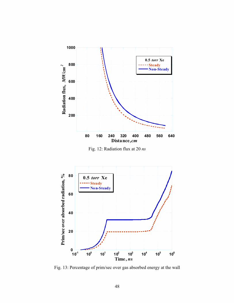
48
200
400
600
800
1000
80 160 240 320 400 480 560 640
SteadyNon-Steady
Rad
iatio
n flu
x, M
W/cm
2
Distance, cm
0.5 torr Xe
Fig. 12: Radiation flux at 20 ns
0
20
40
60
80
10-1 100 101 102 103 104 105 106
SteadyNo n-Steady
Prim
/sec o
ver a
bsor
bed
radi
atio
n, %
Time, ns
0.5 torr Xe
Fig. 13: Percentage of prim/sec over gas absorbed energy at the wall

49
Fig. 14: Absorption coefficient of Xe plasma at 50 eV
Numerical simulations by three models for radiation fluxes in the xenon plasma are essentially different and depend on the quality of the optical coefficients. According to results discussed earlier for the CRE model, during the first 20 ns the temperature of the central zone increases to 280 eV, and by sµ1 , decreases to 100 eV. At such temperatures the nd4 shell is opened, and splitting is taken into account. Within sµ1 after the ions start depositing their energy, the temperature quickly grows to 1 keV ( nd3 shells are opened at that temperature), and then decays to 60 eV by sµ10 .
The spatial distribution of the radiation flux is presented in Fig. 16 for several time steps starting from 10 µs. By that time, the input of new energy to the plasma has been finished, because all ions have deposited their energy either in the plasma or the chamber wall. The fluxes start falling, but the differences in values are still high until 30 µs. At 30 µs the value of radiation flux in the split-lined spectrum is noticeably higher. This condition surely leads to cooling of the plasma. By 100 µs the situation is changed to the opposite: the temperature decrease changes the major ions in the plasma to those corresponding to 5s and 5p shells, and the splitting effect is unimportant to those shells. Nevertheless, at that time, the temperature in the

50
model with HFS lines is higher than that of the line splitting model, and the flux is also higher. As time continues, the fluxes in the central zone gradually decline. By 500 µs the heat effect from the central zone becomes small and comparable to the heat effect in the front of the shock wave due to the adiabatic compression. The front of the radiation fluxes has two distinctive maximums. The large compression is situated in the front of the wave, and the radiation transport in the lined spectrum is optically thin, providing similar results for the models.
Accordingly, the major part of radiation energy is transferred in the lined spectrum. The accuracy and detailed accounting for radiation transfer in the lined spectrum determine the quality of the computations of integral radiation fluxes to the chamber wall, temperature distribution in the plasma, and other important properties and processes in the reactor.
10-11
10-9
10-7
10-5
10-3
10-1
100 101 102 103 104
HFS LinesLine SplittingContinuum
Abs
orpt
ion
coef
ficie
nt,
cm
-1
Photon energy, eV
500 eV, 1015cm-3
10-11
10-9
10-7
10-5
10-3
10-1
200 220 240 260 280 300
HFS LinesLine SplittingContinuum
Abs
orpt
ion
coef
ficie
nt,
cm
-1
Photon energy, eV
3p-3dtransitions
10-9
10-7
10-5
10-3
10-1
101
103
160 180 200 220 240
HFS LinesLine SplittingContinnuum
Abs
orpt
ion
coef
ficie
nt,
cm
-1
Photon energy, eV
4d-5f,6f,6p,7p
3p63dq-3p53dq+1
transitions
10-11
10-9
10-7
10-5
10-3
10-1
101
700 800 900 1000 1100 1200 1300 1400
HFS LinesLine SplittingContinuum
Abs
orpt
ion
coef
ficie
nt,
cm
-1
Photon energy, eV
3d - 4f, 3d - 4p transitions
Fig. 15: Absorption coefficient of Xe plasma at 500 eV

51
0
0.01
0.02
0.03
0.04
0 100 200 300 400 500 600 700
ContinuumHFS LinesLine Splitting
Rad
iatio
n flu
x, M
W/cm
2
Distance, cm
0.05 torr Xe, 100 µs
0
0.2
0.4
0.6
0.8
1
0 100 200 300 400 500 600 700
ContinuumHFS LinesLine Splitting
Rad
iatio
n flu
x, M
W/cm
2
Distance, cm
0.05 torr Xe, 10 µs
0
0.1
0.2
0.3
0.4
0 100 200 300 400 500 600 700
ContinuumHFS LinesLine Splitting
Rad
iatio
n flu
x, M
W/cm
2
Distance, cm
0.05 torr Xe, 30 µs
0
0.0002
0.0004
0.0006
0.0008
0.001
0.0012
0 100 200 300 400 500 600 700
ContinuumHFS LinesLine Splitting
Rad
iatio
n flu
x, M
W/c
m2
Distance, cm
0.05 torr Xe, 500 µs
Fig. 16: Spatial distribution of radiation flux in three models
5.7. Radiation Flux into Wall for Various Initial Pressure Values
In the numerical simulation of the frequency-integrated radiation flux reaching the chamber wall over a long time, one may mark out four typical intervals: direct impact of X-ray radiation until 10 ns, absence of energy surge up to sµ1 , energy deposition of ion fluxes to the chamber gas up to sµ10 , and long-lasting secondary ultraviolet radiation after sµ10 . Fig. 17 shows these intervals, presenting the distribution in time of the radiation flux reaching the chamber wall.
The first interval corresponds to the time for direct impact of X-ray radiation to the chamber wall. The differences in results of several models are small, but they are essential for estimating the later properties and behavior of the plasma in the chamber. The initial gas pressure is a determinative parameter of the following processes. The plasma does not have enough time to be warmed up during the first 10 ns, and it only absorbs hard X-ray radiation from the target. The amount of absorbed energy and the spectrum of this energy are determined by the gas pressure or, to be precise, by the density corresponding to the pressure distribution in the chamber. Fig. 18 shows the initial X-ray spectrum [66] after the target implosion, along with several initial pressure values resulting from the X-ray spectra, which came to the wall after
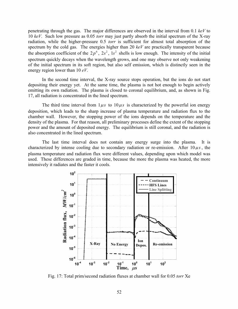
52
penetrating through the gas. The major differences are observed in the interval from 0.1 keV to 10 keV. Such low pressure as 0.05 torr may just partly absorb the initial spectrum of the X-ray radiation, while the higher-pressure 0.5 torr is sufficient for almost total absorption of the spectrum by the cold gas. The energies higher than 20 keV are practically transparent because the absorption coefficient of the 62 p , 22s , 21s shells is low enough. The intensity of the initial spectrum quickly decays when the wavelength grows, and one may observe not only weakening of the initial spectrum in its soft region, but also self emission, which is distinctly seen in the energy region lower than 10 eV.
In the second time interval, the X-ray source stops operation, but the ions do not start depositing their energy yet. At the same time, the plasma is not hot enough to begin actively emitting its own radiation. The plasma is closed to coronal equilibrium, and, as shown in Fig. 17, all radiation is concentrated in the lined spectrum.
The third time interval from sµ1 to sµ10 is characterized by the powerful ion energy deposition, which leads to the sharp increase of plasma temperature and radiation flux to the chamber wall. However, the stopping power of the ions depends on the temperature and the density of the plasma. For that reason, all preliminary processes define the extent of the stopping power and the amount of deposited energy. The equilibrium is still coronal, and the radiation is also concentrated in the lined spectrum.
The last time interval does not contain any energy surge into the plasma. It is characterized by intense cooling due to secondary radiation or re-emission. After sµ10 , the plasma temperature and radiation flux were different values, depending upon which model was used. These differences are graded in time, because the more the plasma was heated, the more intensively it radiates and the faster it cools.
10-6
10-5
10-4
10-3
10-2
10-1
100
101
102
10-4 10-3 10-2 10-1 100 101 102
ContinuumHFS LinesLine Splitting
Rad
iatio
n flu
x,
MW
/cm
2
Time, µs
X-Ray Re-emissionNo Energy IonDepos.
Fig. 17: Total prim/second radiation fluxes at chamber wall for 0.05 torr Xe
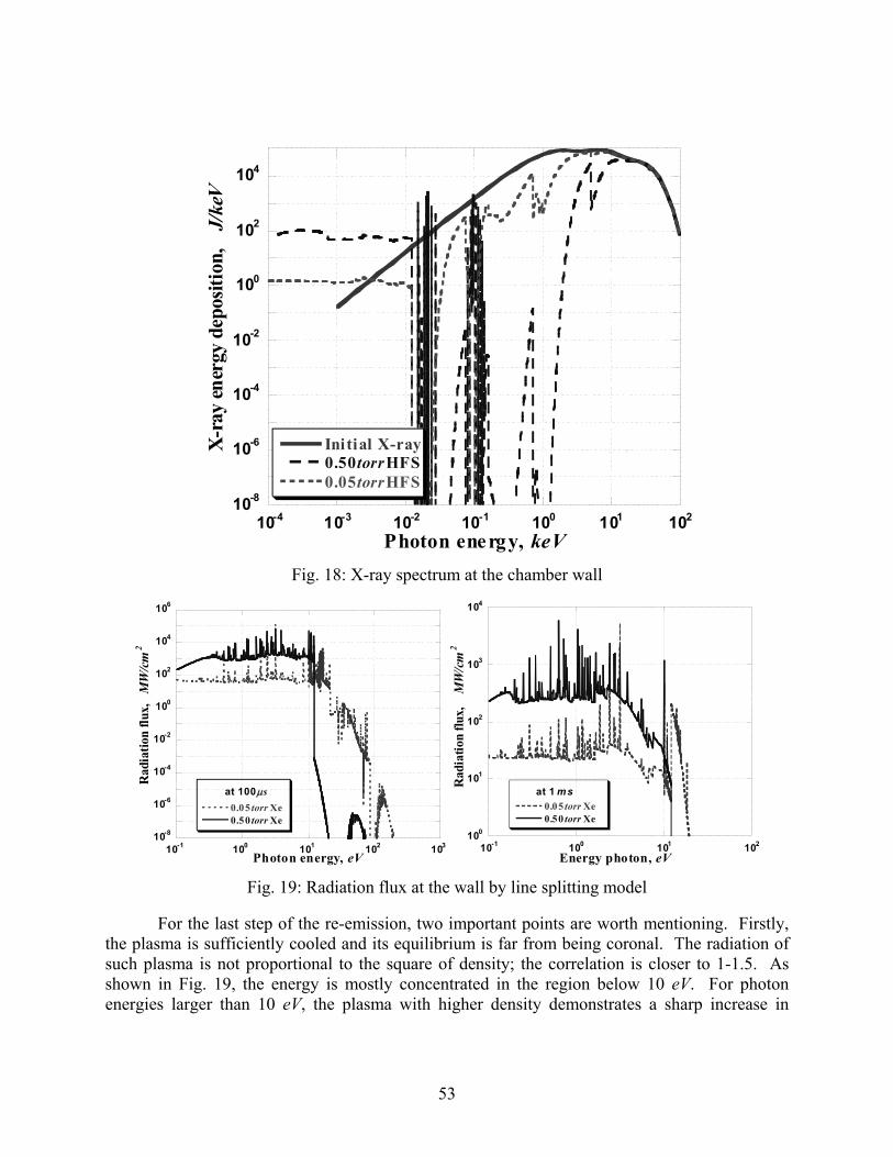
53
10-8
10-6
10-4
10-2
100
102
104
10-4 10-3 10-2 10-1 100 101 102
Initial X-ray0.50 torr HFS0.05 torr HFS
X-r
ay en
ergy
dep
ositi
on,
J/ke
V
Photon energy, keV Fig. 18: X-ray spectrum at the chamber wall
10-8
10-6
10-4
10-2
100
102
104
106
10-1 100 101 102 103
0.05 torr Xe0.50 torr Xe
Rad
iatio
n flu
x,
MW
/cm2
Photon energy, eV
at 100 µs
100
101
102
103
104
10-1 100 101 102
0.05 torr Xe0.50 torr Xe
Rad
iatio
n flu
x,
MW
/cm
2
Energy photon, eV
at 1 ms
Fig. 19: Radiation flux at the wall by line splitting model
For the last step of the re-emission, two important points are worth mentioning. Firstly, the plasma is sufficiently cooled and its equilibrium is far from being coronal. The radiation of such plasma is not proportional to the square of density; the correlation is closer to 1-1.5. As shown in Fig. 19, the energy is mostly concentrated in the region below 10 eV. For photon energies larger than 10 eV, the plasma with higher density demonstrates a sharp increase in
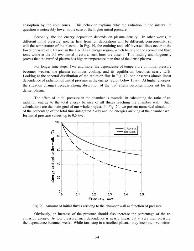
54
absorption by the cold zones. This behavior explains why the radiation in the interval in question is noticeably lower in the case of the higher initial pressure.
Secondly, the ion energy deposition depends on plasma density. In other words, at different initial pressure, specific heat from ion depositions will be different; consequently, so will the temperature of the plasma. In Fig. 19, the emitting and self-inversed lines occur at the lower pressure of 0.05 torr in the 10-100 eV energy region, which belong to the second and third ions, while at the 0.5 torr initial pressure, such lines are absent. This finding unambiguously proves that the rarefied plasma has higher temperature than that of the dense plasma.
For longer time steps, ms1 and more, the dependence of temperature on initial pressure becomes weaker, the plasma continues cooling, and its equilibrium becomes nearly LTE. Looking at the spectral distribution of the radiation flux in Fig. 19, one observes almost linear dependence of radiation on initial pressure in the energy region below 10 eV. At higher energies, the situation changes because strong absorption of the 65p shells becomes important for the denser plasma.
The effect of initial pressure in the chamber is essential in calculating the ratio of re-radiation energy to the total energy balance of all fluxes reaching the chamber wall. Such calculations are the main goal of our whole project. In Fig. 20, we present numerical simulation of the percentage of the total time-integrated X-ray and ion energies arriving at the chamber wall for initial pressure values, up to 0.5 torr.
0
20
40
60
80
100
0 0.1 0.2 0.3 0.4 0.5
X-Ray fluxIon fluxes
Ene
rgy
arri
ved
to th
e w
all,
%
Pressure, torr Fig. 20: Amount of initial fluxes arriving to the chamber wall as function of pressure
Obviously, an increase of the pressure should also increase the percentage of the re-emission energy. At low pressure, such dependence is nearly linear, but at very high pressure, the dependence becomes weak. While ions stop in a rarefied plasma, they keep their velocities,

55
but when the plasma is dense, their velocities are strongly changed. If one takes into account that the dependence of ion energy deposition on ion velocity is a somewhat complicated function with a maximum, then the nonlinear dependence of energy deposition on pressure is more easily understood. Similar behavior is observed for absorption X-ray radiation. At low pressure, a slight pressure increase will lead to an almost linear increase of absorbed energy, but at higher pressure, the energy increase is much less. This result is confirmed by our simulation: the change of initial pressure from 0.025 torr to 0.05 torr gives an almost linear increase of the ratio of the secondary radiation, whereas the further increase of the pressure by one order of magnitude (0.5 torr) changes the percentage of secondary radiation from 13% to 46%, and that for the ions from 24% to 72%.
6. SUMMARY
In our numerical simulation of the properties and behavior of the plasma in an ICF reactor, radiation processes play a crucial role in the energy balance of the system. They define the dynamics of the plasma processes in many respects. In turn, the accurate resolution of the radiation transport problem depends on the level of details in thermodynamic coefficients and opacities, as well as the correctness of the correspondence between (1) such macro parameters of the plasma as temperature, pressure, or density, and (2) the ionization level and other atomic properties.
Using initial parameters and design of the conceptual ICF reactor SOMBRERO, we have shown that successful numerical simulation essentially depends on the theoretical assumptions and the choice of models. Several models are suggested and implemented to calculate the ionization structure of the plasma. We have provided their complex analysis and determined their limits of applicability. The self-consistent, non-steady-state CRE model was found to be essential for successful modeling of the plasma behavior in the ICF reactor at the very initial moments after ignition. The use of the steady-state-model was proven for a wide time range after ion fluxes have arrived and deposited their energy either to the plasma or to the chamber wall. A method for solving the radiation transport equation for spherical geometry was developed and implemented. This method is based upon the approximation of inward/outward directions. Numerical simulations showed that the radiation fluxes significantly depend on the quality and detailed resolution of opacities. In numerical simulation of the radiation transport in the ICF reactor chamber, the finding that the radiation is transferred mainly in the lined spectrum is of no small importance. Using xenon gas for the reference, we calculated opacities for high-Z elements, based upon the modified use of HF and HFS with line splitting methods for computation of atomic properties.
We have additionally shown that the processes occurring in the reactor chamber are not well modeled by simplified methods of simulation of the atomic processes, including calculation of the ionization structure and populations of atomic levels, reductive methods of averaging opacities, and other intuitive estimations, which may often be successfully used in other problems of plasma physics. Preliminary qualitative and quantitative estimations of thermodynamic, optical, and plasma characteristics, obtained in the report, are encouraging. We will work to further improve the atomic models, models of radiation transfer in the lined spectrum, and models of ion energy deposition in the plasma. Additional research is required of

56
initial time steps for detailed simulation of the formation of Auger cascades, non-steady effects, and the influence of external radiation on plasma parameters.
ACKNOWLEDGMENTS
This work is supported by the U.S. Department of Energy, Office of Fusion Energy Sciences and the U.S. Department of Defense.

57
REFERENCES
1. A. Hassanein and I. Konkashbaev, Comprehensive Physical Models and Simulation Package for Plasma/Material Interaction during Plasma Instabilities, J. Nucl. Mater. 273, 326, 1999.
2. A. Hassanein and V. Morozov, Development of Comprehensive and Integrated Models for IFE Cavity Dynamics, Argonne National Laboratory Report ANL-ET/02-04, 2002.
3. V. Sizyuk and A. Hassanein, Hydrodynamic Phenomena of Gas-Filled Chamber due to Target Implosion in IFE Systems, Argonne National Laboratory Report ANL-ET/02-26, 2002.
4. A. Hassanein and I. Konkashbaev, Fragmentation of Liquid-Metal First Wall in ICF Reactors, Proc. 2000 Int. Congress on Plasma Physics (ICPP), Quebec City, Canada, Vol. II, p. 552, 2000.
5. Ya B. Zeldovich, and Yu P. Raizer, Physics of Shock Waves and High-Temperature Hydrodynamic Phenomena, Vol. 1, Academic Press, New York and London, p. 464, 1966.
6. B. N. Bazylev, I. N. Burdonskii, V. I. Tolkach, et al., Laser Particle Beams, 12, 3, 355, 1994.
7. H. A. Bethe, Intermediate Quantum Mechanics, Walter Benjamin, New York, p. 276, 1964.
8. J. C. Slater, Phys. Rev. 81, 385, 1951.
9. F. Herman and S. Skillman, Atomic Structure Calculations, Prentice-Hall, Englewood Cliffs, NJ, 1963.
10. I. I. Sobelman, L. A. Vainstain, and E. A. Yukov, Excitation of Atoms and Broadening of Spectral Lines, Springer-Verlag, New York, 1981.
11. Ch. E. Moore, Atomic Energy Levels as Derived from the Analyses of Optical Spectra, U.S. Dept. Of Commerce, National Bureau of Standards, Washington D.C. p. 3, 1949.
12. B. N. Bazylev, L. V. Golub, G. S. Romanov, and V. I. Tolkach, J. Eng. Phys. Thermophys. 58, 1012-1017, 1990.
13. B. N. Bazylev, L. V. Golub, G. S. Romanov, and V. I. Tolkach, Ibid, 59, 62-65, 1990.
14. G. S. Romanov, and V. I. Tolkach, Ibid, 72, 1039-1046, 1999.
15. M. G. Mayer, Phys. Rev, 60, 184, 1941.
16. D. R. Hartree, The Calculation of Atomic Structures, John Wiley, New York, p. 272, 1957.
17. J. C. Slater, Quantum Theory of Atomic Structures, Vol. II, McGraw-Hill Book Company, Inc., New York, 1960.
18. T. Koopmans, Physica 1, 104, 1934.
19. I. I. Sobelman, Introduction to the Theory of Atomic Spectra, Pergamon Press, New York, 1972.
58
20. T. Holstein, Phys. Rev. 72, 12, 1212, 1947.
21. J. P. Apruzese, et al., J. Quant. Spectrosc. Radiat. Transfer, 23, 479, 1980.
22. P. G. Burke and H. M. Schey, Phys. Rev. 129, 1258, 1963.
23. H. W. Drawin, Report EUP-VEA-FC-383, Assoc. EURATOM-CEA, Frontier-aux-Roses, France, 1967.
24. R. Mewe, Astron. Astrophys. 20, 215, 1972.
25. M. Gryzinski, Phys. Rev. 115, 374, 1959.
26. H. Van Regemorter, Astrophys. J. 132, 906, 1962.
27. W. Lotz, Zs. Physik 232, 101, 1970.
28. A. Burgess, Astrophys. J. 139, 776, 1964.
29. D. W. Savin, Dielectronic Recombination: An Overview of Theory and Experiment, and Some Astrophysical Implications, RevMexAA (Series of Conferences), 9 115-122, 2000.
30. P. Mazzotta, et al., Astron. and Astrophys. 133, 403, 1998.
31. H. R. Griem, Spectral Line Broadening by Plasmas, Academic Press, New York, 1974.
32. J. R. Stallop and K. W. Billman, Plasma Phys. 16, 1187, 1974.
33. W. J. Karzus and R. Latter, Appl. J. Suppl. Ser. 6, 167, 1961.
34. V. I. Derzhiev, A. G. Zhidkov, and G. I. Yakovlenko, Study of Ions in a Nonequilibrium Dense Plasma, Energoatomizdat, Moscow, 1986 (in Russian.)
35. I. A. Sviatoslavsky et al., Fusion Tech. 21, 1470, 1992.
36. R.D. Cowan, The Theory of Atomic Structure and Spectra, Univ. of California Press, 1981.
37. G. Racah, Phys. Rev. 76, 1352, 1949.
38. G. Racah, Phys. Rev. 85, 381, 1952.
39. E. P. Wigner, Quantum Theory of Angular Momentum, in L. C. Biedenharn and H. van Dam, eds, Academic Press, New York, 1965.
40. A. R. Edmonds, Angular Momentum in Quantum Mechanics, 2nd ed., Princeton University Press, Princeton, NJ, 1960.
41. K. Smith and J. W. Stefenson, Argonne National Laboratory Report ANL-5776, 1958.
42. U. Fano, Phys. Rev. 140, A67, 1965.
43. H. A. Jahn, Proc. Roy, Soc. London, A205, 192, 1951.
44. L. Armstrong, Jr., Phys. Rev. 172, 12, 18, 1968.
45. A. P. Jucis and A. J. Savukynas, Mathematical Foundations of the Atomic Theory, Vilnus, p. 480, 1973 (in Russian.)

59
46. C. W. Nielson and G. F. Koster, Spectroscopic Coefficients for the np , nd , and nf Configurations, MIT Press, Cambridge, MA, 1963.
47. B. R. Judd, Operator Techniques in Atomic Spectroscopy, McGraw-Hill, New York, 1963.
48. B. G. Wybourne, Symmetry Principles and Atomic Spectroscopy, Wiley-Interscience, New York, 1970.
49. E. Wigner, Z. Physik 43, 624, 1927.
50. C. Eckart, Rev. Mod. Phys. 2, 305, 1930.
51. H. Marvin, Phys. Rev. 71, 102, 1947.
52. A. Lande, Z. Physik 15, 189, 1923.
53. U. Fano and G. Racah, Irreducible Tensorial Sets, Academic Press, New York, 1959.
54. B. N. Bazylev, V. I. Tolkach, et al., The Calculation of Optical Properties of Atoms and Ions, Kernforschungzentrum Karlsruhe, Interner Bericht, 1994.
55. H. Würz, S. Pestchanyi, I. Landman, B. Bazylev, V. Tolkach, and F. Kappler, Fusion Sci. Technol. 40, N3, 191-246, 2001.
56. Ya B. Zeldovich and Yu P. Raizer, Elements of gas dynamics and the classical theory of shock waves, Academic Press, New York, 1968.
57. A. Schuster, Astrophys, J. 21, 1, 1905.
58. K. Schwarzschild, Göttinger Nachrichten, p. 41, 1906.
59. A. Hassanein and V. Morozov, Fusion Eng. Design 63-64, 609, 2002.
60. L. P. Presnyakov, Charge-exchange of highly charged ions in neutral atoms, in Proc. X Int. Conf. On Phys. Of Electron. And Atom. Collisions, Electronic and Atomic Collisions, North – Holland, p. 407, 1978.
61. T. A. Melhorn, A Finite Material Temperature Model for Ion Energy Deposition in Ion-Driven ICF Targets, Sandia Nat’l Lab. Report SAND80-0038, Albuquerque, NM, 1980.
62. J. Lindhard and M. Scharff, Phys. Rev. 124, 128, 1961.
63. D. A. Callahan-Miller and M. Tabak, Phys. of Plasmas 7, 2083, 2000.
64. D. A. Callahan-Miller and M. Tabak, Nucl. Fusion 39, 11, 1547, 1999.
65. M. Tabak, et al., Target Design Activities for Inertial Fusion Energy at Lawrence Livermore National Laboratory, Proc. 18th IEAE Fusion Energy Conf., Sorento, Italy, October 4-10, 2000.
66. J. Perkins, http://aries.ucsd.edu/ARIES/WDOCS/ARIES-IFE/SPECTRA/

60
Distribution List for ANL-ET/02-23 Internal:
J. P. Allain
J. N. Brooks
H. Drucker
R. Foote
D. Gruen
J. Harmon
A. Hassanein (20)
Z. Insepov
I. Konkashbaev
V. Morozov (5)
J. Norem
R. B. Poeppel
W. Shack
V. A. Sizyuk
S. W. Tam
V. I. Tolkach (5)
R. A. Valentin
TIS Files
External:
DOE-SC (5)
ANL Libraries: ANL-E ANL-W Main Library: Brookhaven National Laboratory
Fermi National Accelerator Laboratory
Lawrence Berkeley National Laboratory
Lawrence Livermore National Laboratory
Los Alamos National Laboratory
Naval Research Laboratory
Sandia National Laboratories
Energy Technology Division Review Committee: H.K. Birnbaum, University of Illinois at Urbana-Champaign
I. -W. Chen, University of Pennsylvania
F. P. Ford, Rexford, N.Y.
S.L. Rohde, University of Nebraska-Lincoln
H.S. Rosenbaum Fremont, CA
S.L. Sass, Cornell University
R. Zoughi, University of Missouri-Rolla

61
External: I. Agurok, Physical Optics Corporation-Torrance, CA M. Akiba, Japan Atomic Energy Research Institute, Japan C. Baker, University of California-San Diego S. Berk, U.S. Department of Energy T. Bernat, Lawrence Livermore National Laboratory G. Besenbruch, General Atomics C. Bibeau, Lawrence Livermore National Laboratory D. Bittner, Lawrence Livermore National Laboratory D. Blackfield, Lawrence Livermore National Laboratory D. Colombant, Naval Research Laboratory B. Cook, Lawrence Livermore National Laboratory J. Dahlburg, General Atomics F. Elsner, General Atomics G. Federici, ITER International Team, Garching, Germany M. Friedman, Naval Research Laboratory J. Gardner, Naval Research Laboratory N. Ghoneim, University of California-Los Angeles J. Giuliani, Naval Research Laboratory D. Goodin, General Atomics-San Diego C. Halvorson, Schafer Laboratories R. Hawryluk, Princeton Plasma Physics Laboratory D. Haynes, Los Alamos National Laboratory F. Hegeler, Naval Research Laboratory J. Hoffer, Los Alamos National Laboratory J. Hunn, Oak Ridge National Laboratory S. A. Khalik, Georgia Tech Y. Kozaki, Osaka University, Japan P. Lamarche, Princeton Plasma Physics Laboratory B. Lehmberg, Naval Research Laboratory J. Lindl, Lawrence Livermore National Laboratory Y. Martynenko, Kurchatov Institute, Russia W. Meier, Lawrence Livermore National Laboratory M. Monsler, Schafer Laboratories- Livermore, CA M. Myers, Naval Research Laboratory G. Nardella, U.S. Department of Energy

62
External:(cont)
A. Nobile, Los Alamos National Laboratory R. Nygren, Sandia National Laboratories-Albuquerque S. Obenschain, Naval Research Laboratory A. Opdenaker, U.S. Department of Energy J. Perkins, Lawrence Livermore National Laboratory R. Peterson, Los Alamos National Laboratory R. Petzold, General Atomics F. Powell, Luxel Corporation - Friday Harbor, WA J. Sater, Lawrence Livermore National Laboratory M. Sawan, University of Wisconsin J. Sethian, Naval Research Laboratory R. Schneider, U.S. Department of Energy D. Schroen, Sandia National Laboratories K. Schultz, General Atomics M. Seki, Japan Atomic Energy Research Institute, Japan J. Shillito, Schafer Laboratories-Livermore, CA C. Skinner, Princeton Plasma Physics Laboratory L. Snead, Oak Ridge National Laboratory D. Steiner, Rensselaer Polytechnic Institute J. Swadener, Los Alamos National Laboratory T. Norimatsu, Institute of Laser Engineering, Osaka University, Japan M. Tillack, University of California, San Diego Y. Ueda, Osaka University, Japan L. Wagner, Boeing, St. Louis D. Weidenheimer, Titan Corporation M. Wolford, Naval Research Laboratory S. Zinkle, Oak Ridge National Laboratory Bibliothek, Max-Planck-Institute für Plasmaphysik, Germany C.E.A. Library, Fontenay-aux-Roses, France Librarian, Culham Laboratory, England Thermonuclear Library, Japan Atomic Energy Research Institute, Japan University of Wisconsin Library