ankit sharma(dsp)
TRANSCRIPT

8/6/2019 Ankit sharma(dsp)
http://slidepdf.com/reader/full/ankit-sharmadsp 1/33
Digital
Signal
Processing
BY:- Ankit Sharma
Roll No:- 0657013108
BTECH(IT)
8/6/2019 Ankit sharma(dsp)
http://slidepdf.com/reader/full/ankit-sharmadsp 2/33
Experiment No. 1
Aim: To study MATLAB and various commands and file types associated with it and henceappreciate the use of MATLAB in signal processing.
THEORY
MATLAB (short for Matrix Laboratory) is a special purpose computer program organized to
perform engineering and scientific calculations.
MATLAB has many advantages compared to conventional computer languages for technical
problem solving .Among them are:
1) Ease of use:->Programs may be easily written and modified with the built in integrateddevelopment environment and debugged with the MATLAB debugger. Because the language is
so easy to use, it is ideal for the rapid prototyping of new programs.
2) Platform independence:->MATLAB is supported on many different computer systems ,
providing a large measure of platform independence. As a result, programs written in MATLAB
can migrate to new platforms when the needs of the user change.
3) Predefined functions:->MATLAB comes complete with an extensive library of predefined
functions that provide tested and pre-packaged solutions to many basic technical tasks.
4) Device independent plotting:->The plots and images can be displaced on any graphical outputdevice supported by the computer on which MATLAB is running. This capability makes
MATLAB an outstanding tool for visualizing technical data.
5) Graphical user interface:->MATLAB includes tools that allow a programmer to interactively
construct a graphical user interface for program.
6) MATLAB compiler:-> MATLAB¶s flexibility and platform independence is achieved by
compiling MATLAB programs into a device independent p-code and then interpreting the p-
code at run time.
Commands & Essential functions in MATLAB:
y clc- clear the command window only.
y clear-removes all variables from workspace.
y clear all- removes all variables, globals & functions.

8/6/2019 Ankit sharma(dsp)
http://slidepdf.com/reader/full/ankit-sharmadsp 3/33
y Ls-listing of cursor directory.
y Pwd- present, working, directory.
y Load-load data from a file
y «-continues a MATLAB statement in the following line.
y Date-current date
y Title-adds a title to a plot
y Save-save data from workspace in a file.
y Print-prints a figure window.
y Max(x)-returns the maximum value in vector x, and optionally the location of that value.
y Min(x)-returns the minimum value in vector x, and optionally the location of that value.
y Log(x)-calculates natural logarithm of x.
y Help«.(command name)-give brief description of asked command.
y doc«.(command name)-full description.
y Whos-list all variables in current workspace,size.edit-matlab editor «.etc.
y edit-matlab editor
y Size(a)-return size of matrix a.
y Length(a)-maximum dimension of matrix.
y A¶-to change column vector to row.
y Logspace-generates logarithmic generated spaced vectors.
y Find(a)-returns indexes (row and column no. of non-zero elements).
y Disp-accepts an array arguments and displays the value .
y Abs(x)-calculates the absolute value of x.
y Ans-default variable used to store the result of expression not assigned to another
variable.
y Acos(x)-calculates inverse cosine of x.
y Asin(x)- calculates inverse sine of x.
y Atan(x)- calculates inverse tangent of x.
y Ceil(x)-rounds x to the nearest integer towards positive infinity.
y Char-converts a matrix of nos. into a character string.
y Clock-current time
y Cos(x)-calculates cosine of x.
y Eps-represents machine precision.
y Inf-represents machine infinity.
y Mod(n,m)-remainder or modulo function
y Sqrt-calculates square of a no.

8/6/2019 Ankit sharma(dsp)
http://slidepdf.com/reader/full/ankit-sharmadsp 4/33
Experiment No. 2
Aim:Write a program to develop elementary signal function modules (m-files) for unit sample,
unit step, exponential and unit ramp sequences.
THEORY
Exponential Function:
A function f(x)=ex
is defined as:
0<f(x)�1; for -��x�0
1�f(x)<�; for 0�x��
Unit impulse Function:
Unit impulse is a signal that is 0 everywhere except at n=0 where it is 1. In discrete time domain
the unit impulse signal is defined as:
�(n) = 1; n=0
= 0; elsewhere
Unit Step Function:
The integral of the impulse function is a unit step signal. In discrete time unit step signal is
defined as:
U(n) = 1; n>=0
= 0; n<0
Ramp signal:
Ramp signal increases linearly with sample number n. It is defined as
R(n) = n; n>=0
= 0; n<0

8/6/2019 Ankit sharma(dsp)
http://slidepdf.com/reader/full/ankit-sharmadsp 5/33
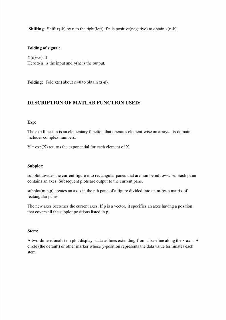
DESCRIPTION OF MATLAB FUNCTION USED:
Exp:
The exp function is an elementary function that operates element-wise on arrays. Its domain
includes complex numbers.
Y = exp(X) returns the exponential for each element of X.
Subplot:
subplot divides the current figure into rectangular panes that are numbered rowwise. Each pane
contains an axes. Subsequent plots are output to the current pane.
subplot(m,n,p) creates an axes in the pth pane of a figure divided into an m-by-n matrix of
rectangular panes.
The new axes becomes the current axes. If p is a vector, it specifies an axes having a position
that covers all the subplot positions listed in p.
Stem:
A two-dimensional stem plot displays data as lines extending from a baseline along the x-axis. Acircle (the default) or other marker whose y-position represents the data value terminates each
stem.
stem(X,Y) plots X versus the columns of Y. X and Y must be vectors or matrices of the same
size. Additionally, X can be a row or a column vector and Y a matrix with length(X) rows.
Xlabel:
xlabel('string') labels the x-axis of the current axes.
Ylabel:
ylabel('string') labels the y-axis of the current axes.

8/6/2019 Ankit sharma(dsp)
http://slidepdf.com/reader/full/ankit-sharmadsp 6/33
PROGRAM:
%TO PLOT EXPONENTIAL SIGNAL
t=0:7;
a=1;
y2=exp(a*t);
subplot(2,2,1);
stem(t,y2);
ylabel('amplitude-->');
xlabel('n-->')
%TO PLOT UNIT SAMPLE SIGNAL
clc;
clear all;
clear all;
t=-2:1:2;
y=[zeros(1,2),ones(1,1),zeros(1,2)];
subplot(2,2,2);
stem(t,y);
ylabel('amplitude-->');
xlabel('n-->');
8/6/2019 Ankit sharma(dsp)
http://slidepdf.com/reader/full/ankit-sharmadsp 7/33
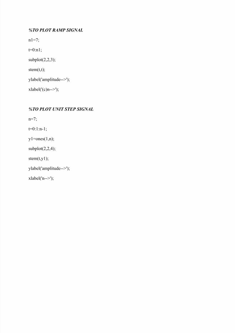
%TO PLOT RAMP SIGNAL
n1=7;
t=0:n1;
subplot(2,2,3);
stem(t,t);
ylabel('amplitude-->');
xlabel('(c)n-->');
%TO PLOT UNIT STEP SIGNAL
n=7;
t=0:1:n-1;
y1=ones(1,n);
subplot(2,2,4);
stem(t,y1);
ylabel('amplitude-->');
xlabel('n-->');

8/6/2019 Ankit sharma(dsp)
http://slidepdf.com/reader/full/ankit-sharmadsp 8/33
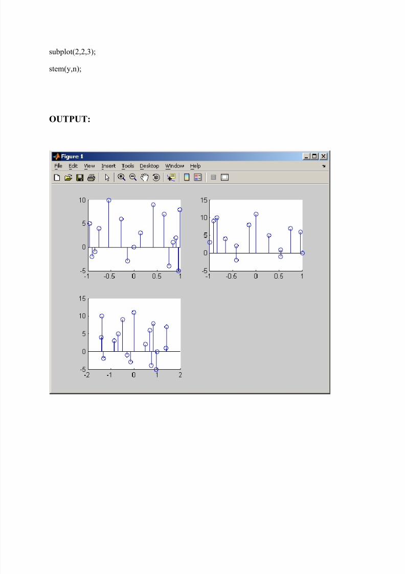
OUTPUT:

8/6/2019 Ankit sharma(dsp)
http://slidepdf.com/reader/full/ankit-sharmadsp 9/33
Experiment No. 3
Aim:Write a program to develop program modules based on operation on sequences like signal
shifting,signal folding,signal addition and signal multiplication.
THEORY Signal processing is group of basic operations applied to an input signal resulting in another
signal as the output. There are various operations which can be performed on a signal.
Signal addition:
{x1(n)}+{x2(n)}={x1(n)+x2(n)}
Summation: Sum all the values of the sequence to obtain the value of the output at a given
time.
Signal multiplication:
{x1(n)}*{x2(n)}={x1(n)*x2(n)}
Multiplication: Multiply x1(n) by x2(n) to obtain the value of the output sequence.
Scaling of signal:
S*{x(n)}={s*x(n)}
Shifting of signal:
The shift signal takes the input sequence and shifts the values by an increment of the independent
variable. The shifting may delay or advance the sequences in time.
Y(n)={x(n-k)}
8/6/2019 Ankit sharma(dsp)
http://slidepdf.com/reader/full/ankit-sharmadsp 10/33
Shifting: Shift x(-k) by n to the right(left) if n is positive(negative) to obtain x(n-k).
Folding of signal:
Y(n)=x(-n)
Here x(n) is the input and y(n) is the output.
Folding: Fold x(n) about n=0 to obtain x(-n).
DESCRIPTION OF MATLAB FUNCTION USED:
Exp:
The exp function is an elementary function that operates element-wise on arrays. Its domain
includes complex numbers.
Y = exp(X) returns the exponential for each element of X.
Subplot:
subplot divides the current figure into rectangular panes that are numbered rowwise. Each pane
contains an axes. Subsequent plots are output to the current pane.
subplot(m,n,p) creates an axes in the pth pane of a figure divided into an m-by-n matrix of
rectangular panes.
The new axes becomes the current axes. If p is a vector, it specifies an axes having a position
that covers all the subplot positions listed in p.
Stem:
A two-dimensional stem plot displays data as lines extending from a baseline along the x-axis. A
circle (the default) or other marker whose y-position represents the data value terminates each
stem.

8/6/2019 Ankit sharma(dsp)
http://slidepdf.com/reader/full/ankit-sharmadsp 11/33
stem(X,Y) plots X versus the columns of Y. X and Y must be vectors or matrices of the same
size. Additionally, X can be a row or a column vector and Y a matrix with length(X) rows.
Xlabel:
xlabel('string') labels the x-axis of the current axes.
Ylabel:
ylabel('string') labels the y-axis of the current axes.
Sin:
The sin function operates element-wise on arrays. The function's domains and ranges include
complex values. All angles are in radians.
Y = sin(X) returns the circular sine of the elements of X.
Cos:
The cos function operates element-wise on arrays. The function's domains and ranges include
complex values. All angles are in radians.
Y = cos(X) returns the circular cosine for each element of X.
Max:
C = max(A) returns the largest elements along different dimensions of an array.
Min:
C = min(A) returns the smallest elements along different dimensions of an array.

8/6/2019 Ankit sharma(dsp)
http://slidepdf.com/reader/full/ankit-sharmadsp 12/33
Zeros:
Creates an array of all zeros.
B = zeros(m,n) or B = zeros([m n]) returns an m-by-n matrix of zeros.
Fliplr:
B = fliplr(A) returns A with columns flipped in the left-right direction, that is, about a vertical
axis.
Disp:
disp(X) displays an array, without printing the array name. If X contains a text string, the stringis displayed.
PROGRAM:
%% Signal addition
n1=[-5:10];
n2=[-2:11];
x1=sin(n1);
x2=cos(n2);
subplot(2,2,1);stem(x1,n1);
subplot(2,2,2);stem(x2,n2);
n=min(min(n1),min(n2)): max(max(n1),max(n2));
y1=zeros(1,length(n));
y2=y1;
y2(find((n>=min(n2))&(n<=max(n2))==1))=x2;
y1(find((n>=min(n1))&(n<=max(n1))==1))=x1;
y=y1+y2;
8/6/2019 Ankit sharma(dsp)
http://slidepdf.com/reader/full/ankit-sharmadsp 13/33
subplot(2,2,3);
stem(y,n);
OUTPUT:

8/6/2019 Ankit sharma(dsp)
http://slidepdf.com/reader/full/ankit-sharmadsp 14/33
%% Signal multiplication
n1=[-5:10];
n2=[-2:11];
x1=sin(n1);
x2=cos(n2);
n=min(min(n1),min(n2)): max(max(n1),max(n2));
y1=zeros(1,length(n));
y2=y1;
y2(find((n>=min(n2))&(n<=max(n2))==1))=x2;
y1(find((n>=min(n1))&(n<=max(n1))==1))=x1;
y=y1.*y2;
stem(n,y);
OUTPUT:

8/6/2019 Ankit sharma(dsp)
http://slidepdf.com/reader/full/ankit-sharmadsp 15/33
%% Signal Shifting
a=8;
n1=[3:18];
x1=n1;
subplot(1,2,1);stem(n1,x1);
n=a+n1;
y=x1;
subplot(1,2,2);stem(n,y);
OUTPUT:
8/6/2019 Ankit sharma(dsp)
http://slidepdf.com/reader/full/ankit-sharmadsp 16/33
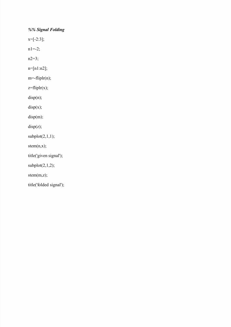
%% Signal Folding
x=[-2:3];
n1=-2;
n2=3;
n=[n1:n2];
m=-fliplr(n);
z=fliplr(x);
disp(n);
disp(x);
disp(m);
disp(z);
subplot(2,1,1);
stem(n,x);
title('given signal');
subplot(2,1,2);
stem(m,z);
title('folded signal');

8/6/2019 Ankit sharma(dsp)
http://slidepdf.com/reader/full/ankit-sharmadsp 17/33
OUTPUT:
8/6/2019 Ankit sharma(dsp)
http://slidepdf.com/reader/full/ankit-sharmadsp 18/33
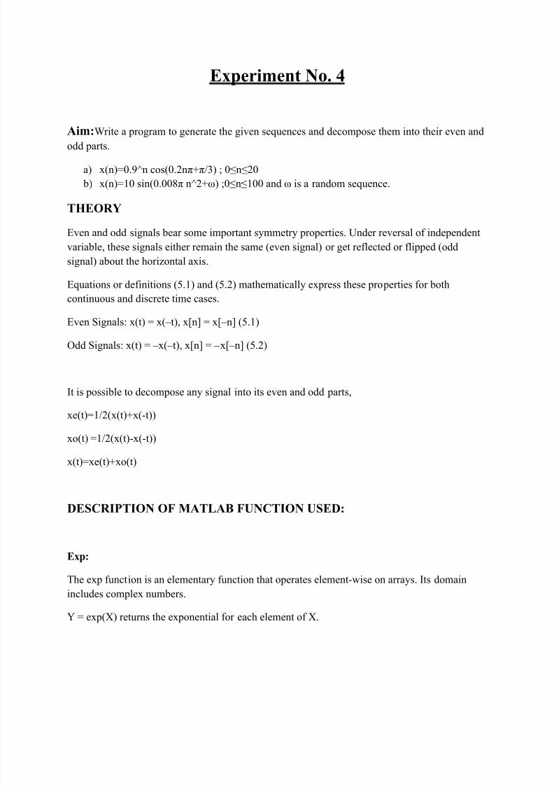
Experiment No. 4
Aim:Write a program to generate the given sequences and decompose them into their even and
odd parts.
a) x(n)=0.9^n cos(0.2n+/3) ; 0�n�20
b) x(n)=10 sin(0.008 n^2+) ;0�n�100 and is a random sequence.
THEORY
Even and odd signals bear some important symmetry properties. Under reversal of independent
variable, these signals either remain the same (even signal) or get reflected or flipped (odd
signal) about the horizontal axis.
Equations or definitions (5.1) and (5.2) mathematically express these properties for both
continuous and discrete time cases.
Even Signals: x(t) = x(±t), x[n] = x[±n] (5.1)
Odd Signals: x(t) = ±x(±t), x[n] = ±x[±n] (5.2)
It is possible to decompose any signal into its even and odd parts,
xe(t)=1/2(x(t)+x(-t))
xo(t) =1/2(x(t)-x(-t))
x(t)=xe(t)+xo(t)
DESCRIPTION OF MATLAB FUNCTION USED:
Exp:
The exp function is an elementary function that operates element-wise on arrays. Its domain
includes complex numbers.
Y = exp(X) returns the exponential for each element of X.
8/6/2019 Ankit sharma(dsp)
http://slidepdf.com/reader/full/ankit-sharmadsp 19/33
Subplot:
subplot divides the current figure into rectangular panes that are numbered rowwise. Each pane
contains an axes. Subsequent plots are output to the current pane.
subplot(m,n,p) creates an axes in the pth pane of a figure divided into an m-by-n matrix of rectangular panes.
The new axes becomes the current axes. If p is a vector, it specifies an axes having a position
that covers all the subplot positions listed in p.
Stem:
A two-dimensional stem plot displays data as lines extending from a baseline along the x-axis. A
circle (the default) or other marker whose y-position represents the data value terminates each
stem.
stem(X,Y) plots X versus the columns of Y. X and Y must be vectors or matrices of the same
size. Additionally, X can be a row or a column vector and Y a matrix with length(X) rows.
Xlabel:
xlabel('string') labels the x-axis of the current axes.
Ylabel:
ylabel('string') labels the y-axis of the current axes.
Clf:
clf deletes from the current figure all graphics objects whose handles are not hidden (i.e., their
HandleVisibility property is set to on).
Figure:
figure(h) does one of two things, depending on whether or not a figure with handle h exists. If h
is the handle to an existing figure, figure(h) makes the figure identified by h the current figure,

8/6/2019 Ankit sharma(dsp)
http://slidepdf.com/reader/full/ankit-sharmadsp 20/33
makes it visible, and raises it above all other figures on the screen. The current figure is the target
for graphics output. If h is not the handle to an existing figure, but is an integer, figure(h) creates
a figure and assigns it the handle h. figure(h) where h is not the handle to a figure, and is not an
integer, is an error.
Cos:
The cos function operates element-wise on arrays. The function's domains and ranges include
complex values. All angles are in radians.
Y = cos(X) returns the circular cosine for each element of X.
Fliplr:
B = fliplr(A) returns A with columns flipped in the left-right direction, that is, about a vertical
axis.
a)
PROGRAM:
n=[0:20];
x=(0.9.^n).*cos((0.2.*n.*pi)+(pi/3));
[xe,xo,m]=evenodd(x,n);
figure(1),clf;
subplot(2,2,1);stem(n,x);
title('Main');
subplot(2,2,2);stem(m,xo);
title('ODD');
subplot(2,2,3);stem(m,xe);
title('EVEN');

8/6/2019 Ankit sharma(dsp)
http://slidepdf.com/reader/full/ankit-sharmadsp 21/33
FUNCTION:
function[xo,xe,m]=evenodd(x,n)
if any(imag(x)~=0)
error('X is not a real sequence');
end
m=-fliplr(n);
m1=min([m,n]); m2=max([m,n]);
m=m1:m2;
nm=n(1)-m(1); n1=1:length(n);
x1=zeros(1,length(m));
x1(n1+nm)=x; x=x1;
xe=0.5*(x+fliplr(x));
xo=0.5*(x-fliplr(x));
OUTPUT:

8/6/2019 Ankit sharma(dsp)
http://slidepdf.com/reader/full/ankit-sharmadsp 22/33
b)
PROGRAM:
n=[0:100];
x=10.*sin(0.008.*pi.*(n.^2)+randn(1,101));
[xe,xo,m]=evenodd(x,n);
figure(1),clf;
subplot(2,2,1);stem(n,x);
title('Main');
subplot(2,2,2);stem(m,xo);
title('ODD');
subplot(2,2,3);stem(m,xe);
title('EVEN');
function:
function[xo,xe,m]=evenodd(x,n)
if any(imag(x)~=0)
error('X is not a real sequence');
end
m=-fliplr(n);
m1=min([m,n]); m2=max([m,n]);
m=m1:m2;
nm=n(1)-m(1); n1=1:length(n);
x1=zeros(1,length(m));
x1(n1+nm)=x; x=x1;
xe=0.5*(x+fliplr(x));xo=0.5*(x-fliplr(x));

8/6/2019 Ankit sharma(dsp)
http://slidepdf.com/reader/full/ankit-sharmadsp 23/33
OUTPUT:

8/6/2019 Ankit sharma(dsp)
http://slidepdf.com/reader/full/ankit-sharmadsp 24/33
Experiment No. 6
Aim: Write a program to show the application of cross correlation in comparing the signals.
THEORY
In signal processing, cross-correlation is a measure of similarity of two waveforms as a function
of a time-lag applied to one of them. This is also known as a sliding dot product or inner-
product . It is commonly used to search a long duration signal for a shorter, known feature. It also
has applications in pattern recognition, single particle analysis, electron tomographic
averaging, cryptanalysis, and neurophysiology.
For continuous functions, f and g , the cross-correlation is defined as:
where f * denotes the complex conjugate of f .
Similarly, for discrete functions, the cross-correlation is defined as:
DESCRIPTION OF MATLAB FUNCTION USED:
Exp:
The exp function is an elementary function that operates element-wise on arrays. Its domain
includes complex numbers.
Y = exp(X) returns the exponential for each element of X.
Subplot:
subplot divides the current figure into rectangular panes that are numbered rowwise. Each pane
contains an axes. Subsequent plots are output to the current pane.

8/6/2019 Ankit sharma(dsp)
http://slidepdf.com/reader/full/ankit-sharmadsp 25/33
subplot(m,n,p) creates an axes in the pth pane of a figure divided into an m-by-n matrix of
rectangular panes.
The new axes becomes the current axes. If p is a vector, it specifies an axes having a position
that covers all the subplot positions listed in p.
Stem:
A two-dimensional stem plot displays data as lines extending from a baseline along the x-axis. A
circle (the default) or other marker whose y-position represents the data value terminates each
stem.
stem(X,Y) plots X versus the columns of Y. X and Y must be vectors or matrices of the same
size. Additionally, X can be a row or a column vector and Y a matrix with length(X) rows.
Xlabel:
xlabel('string') labels the x-axis of the current axes.
Ylabel:
ylabel('string') labels the y-axis of the current axes.
Xcorr:
c = xcorr(x,y) returns the cross-correlation sequence in a length 2*N-1 vector, where x and y are
length N vectors (N>1).
If x and y are not the same length, the shorter vector is zero-padded to the length of the longer
vector. By default, xcorr computes raw correlations with no normalization.

8/6/2019 Ankit sharma(dsp)
http://slidepdf.com/reader/full/ankit-sharmadsp 26/33
PROGRAM:
x=[1,2,3,4];
y=[4,3,2,1];
nx=[0:8];
[c,lags]=xcorr(x,y);
subplot(1,1,1);
stem(lags,c);
xlabel('n');
ylabel('a');
OUTPUT:
8/6/2019 Ankit sharma(dsp)
http://slidepdf.com/reader/full/ankit-sharmadsp 27/33
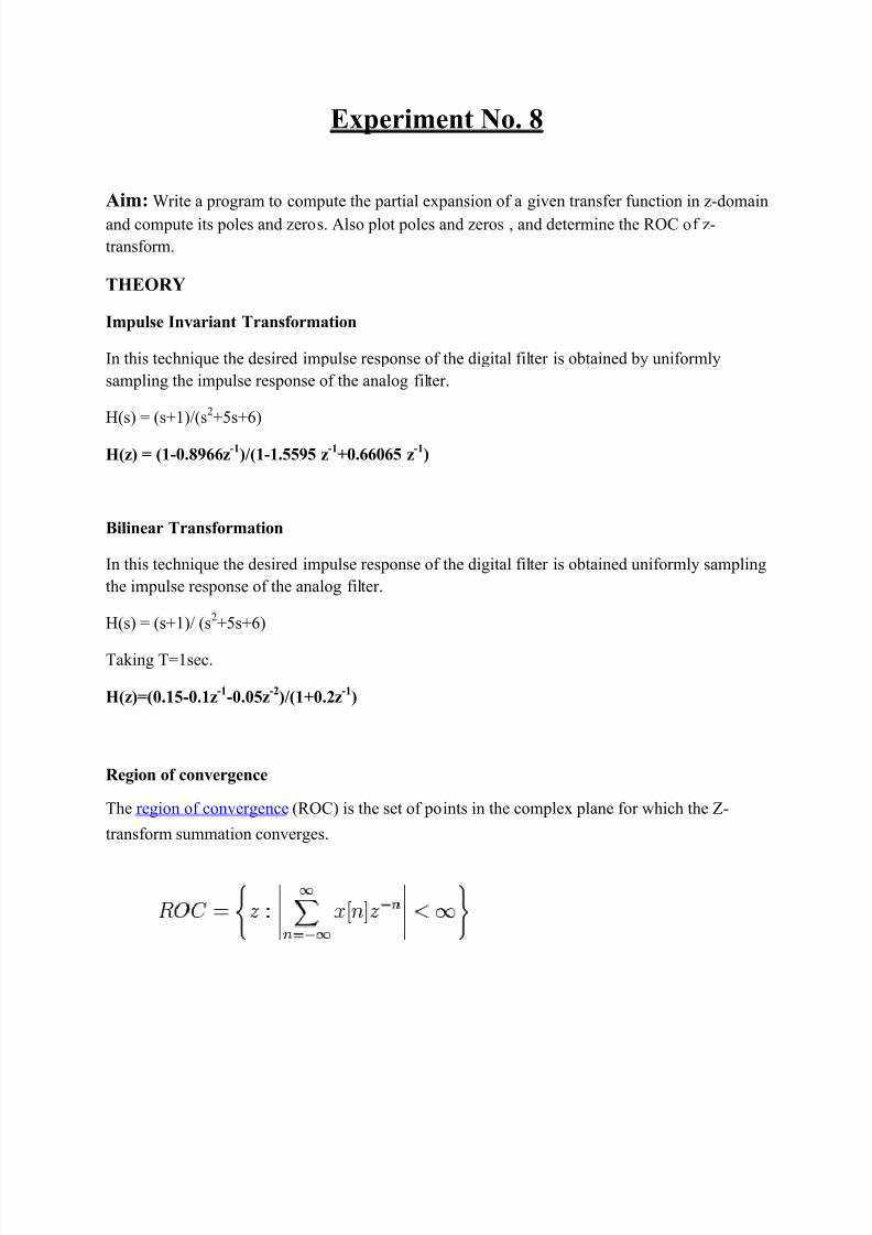
Experiment No. 8
Aim: Write a program to compute the partial expansion of a given transfer function in z-domain
and compute its poles and zeros. Also plot poles and zeros , and determine the ROC of z-
transform.
THEORY
Impulse Invariant Transformation
In this technique the desired impulse response of the digital filter is obtained by uniformly
sampling the impulse response of the analog filter.
H(s) = (s+1)/(s2+5s+6)
H(z) = (1-0.8966z-1
)/(1-1.5595 z-1
+0.66065 z-1
)
Bilinear Transformation
In this technique the desired impulse response of the digital filter is obtained uniformly sampling
the impulse response of the analog filter.
H(s) = (s+1)/ (s2+5s+6)
Taking T=1sec.
H(z)=(0.15-0.1z-1
-0.05z-2
)/(1+0.2z-1
)
Region of convergence
The region of convergence (ROC) is the set of points in the complex plane for which the Z-
transform summation converges.

8/6/2019 Ankit sharma(dsp)
http://slidepdf.com/reader/full/ankit-sharmadsp 28/33
DESCRIPTION OF MATLAB FUNCTION USED:
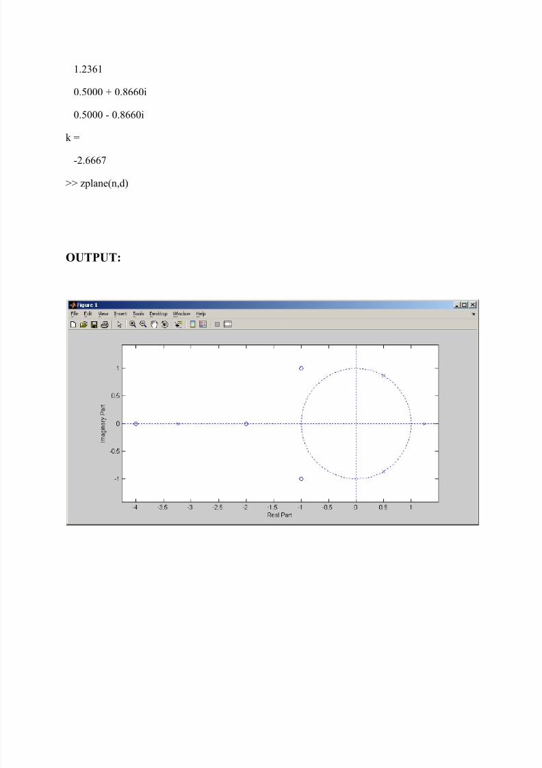
Zplane:
This function displays the poles and zeros of quantized filters, as well as the poles and zeros of
the associated unquantized reference filter.
Residue:
[r,p,k] = residue(b,a) finds the residues, poles, and direct terms of a partial fraction expansion of
the ratio of two polynomials, b(z) and a(z). Vectors b and a specify the coefficients of the
polynomials of the discrete-time system b(z)/a(z) in descending powers of z
PROGRAM:
>> n=[2 16 44 56 32]
n =
2 16 44 56 32
>> d=[3 3 -15 18 -12]
d =
3 3 -15 18 -12
>> [r,p,k]=residue(n,d)
r =
-0.0177
9.4914
-3.0702 + 2.3398i
-3.0702 - 2.3398i
p =
-3.2361
8/6/2019 Ankit sharma(dsp)
http://slidepdf.com/reader/full/ankit-sharmadsp 29/33
1.2361
0.5000 + 0.8660i
0.5000 - 0.8660i
k =
-2.6667
>> zplane(n,d)
OUTPUT:

8/6/2019 Ankit sharma(dsp)
http://slidepdf.com/reader/full/ankit-sharmadsp 30/33
Experiment No. 7
Aim: To compute the circular convolution of two sequences using MATLAB functions andusing the fold, shift and multiply procedure, then compare the result with that obtained using
DFT & IDFT.
THEORY
Let x1(n) and x2(n) are finite duration sequences both of length N with DFTs X1(k) and
X2(k).Now we find a sequence x3(n) for which the DFT is X3(k), where
X3(K)=X1(K)*X2(K)
We know from earlier computations that
N-1
X3(n)= x1(m)x2(n-m)N
m=0
This equation represents circular convolution of x1(n) and x2(n) which is represented as
X3( n)=x1(n) x x2(n)
We find that DFT of:
DFT[x1(n) x2(n)]=X1(K)*X2(K)
PROGRAM:
%% circular convolution
clc;
clear all;
close all;
N
N
8/6/2019 Ankit sharma(dsp)
http://slidepdf.com/reader/full/ankit-sharmadsp 31/33
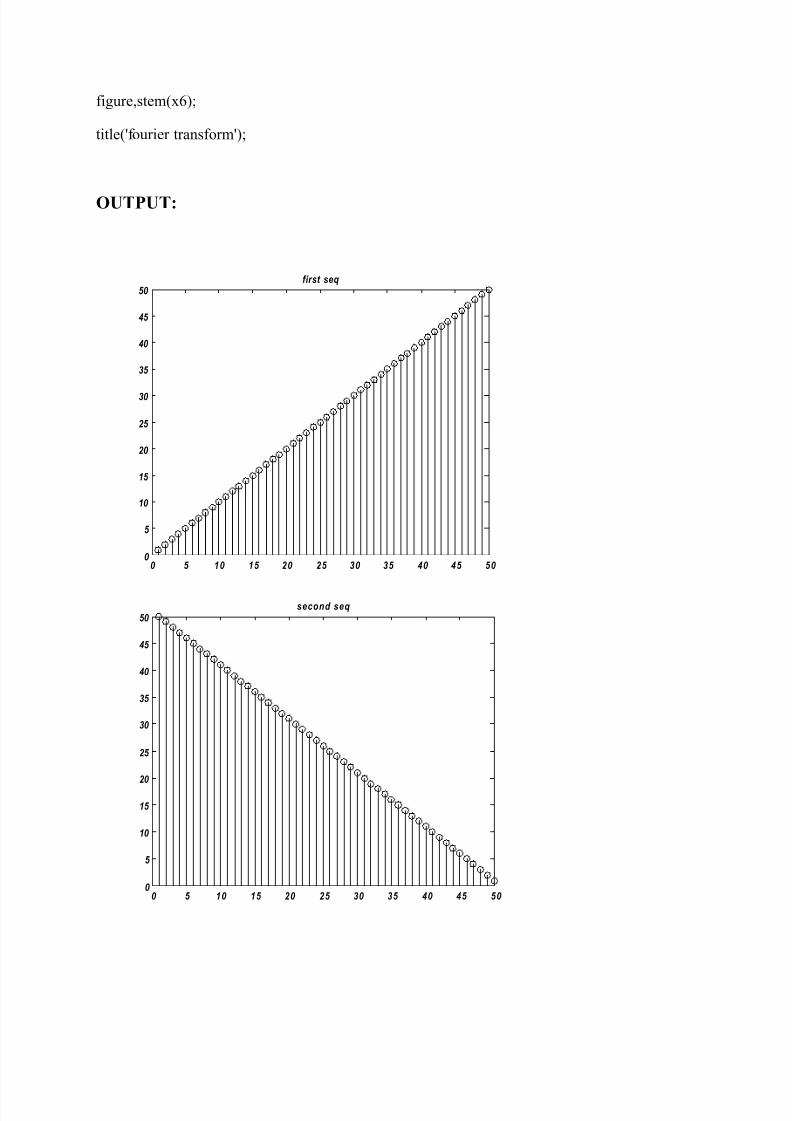
n=50;
x1=1:n;
figure,stem(x1);
title('first seq');
x2=n:-1:1;
figure,stem(x2);
title('second seq');
x3=cconv(x1,x2,n);
figure,stem(x3);
title('Circular convolution using conv');
x4=fliplr(x1);
x4=circshift(x4,[0,1]);
for i=1:n
x5(i)=sum(x2.*circshift(x4,[0,i-1]));
end
figure,stem(x5);
title(' circular convolution using shift for n multiply procedure');
x6=fft(x1).*fft(x2);
x6==ifft(x6);
8/6/2019 Ankit sharma(dsp)
http://slidepdf.com/reader/full/ankit-sharmadsp 32/33
figure,stem(x6);
title('fourier transform');
OUTPUT:
0 5 10 15 20 25 30 35 40 45 50 0
5
10
15
20
25
30
35
40
45
50 first seq
0 5 10 15 20 25 30 35 40 45 50 0
5
10
15
20
25
30
35
40
45
50 second seq

8/6/2019 Ankit sharma(dsp)
http://slidepdf.com/reader/full/ankit-sharmadsp 33/33