anintroductionto inla withacomparisonto jagsstatistica.it/gianluca/talks/inla.pdf · gianluca baio...
TRANSCRIPT

An introduction to INLA with a comparison to JAGS
Gianluca Baio
University College LondonDepartment of Statistical Science
(Thanks to Havard Rue, University of Science and Technology Trondheim, Norway)
Bayes 2013
Rotterdam, Tuesday 21 May 2013
Gianluca Baio ( UCL) Introduction to INLA Bayes 2013, 21 May 2013 1 / 92

Laplace’s liberation army (?)
Gianluca Baio ( UCL) Introduction to INLA Bayes 2013, 21 May 2013 2 / 92

Laplace’s liberation army (?)
Gianluca Baio ( UCL) Introduction to INLA Bayes 2013, 21 May 2013 2 / 92

Outline of presentation
1 9.00 – 9.45: (Quick & moderately clean) introduction to Bayesiancomputation
– MCMC– Latent Gaussian models– Gaussian Markov Random Fields
2 9.45 – 10.00: Coffee break
3 10.00 – 10.45: Introduction to INLA
– Basic ideas– Some details– A simple example
4 10.45 – 11.00: Coffee break
5 11.00 – 12.00: Using the package R-INLA
– How does it work?– Some simple examples– (Slightly) more complex examples
Gianluca Baio ( UCL) Introduction to INLA Bayes 2013, 21 May 2013 3 / 92

(Quick & moderately clean)introduction to Bayesian
computation
Gianluca Baio ( UCL) Introduction to INLA Bayes 2013, 21 May 2013 4 / 92

Bayesian computation
• In a (very small!) nutshell, Bayesian inference boils down to the computationof posterior and/or predictive distributions
p(θ | y) =p(y | θ)p(θ)∫p(y | θ)p(θ)dθ
p(y∗ | y) =
∫p(y∗ | θ)p(θ | y)dθ
Gianluca Baio ( UCL) Introduction to INLA Bayes 2013, 21 May 2013 5 / 92

Bayesian computation
• In a (very small!) nutshell, Bayesian inference boils down to the computationof posterior and/or predictive distributions
p(θ | y) =p(y | θ)p(θ)∫p(y | θ)p(θ)dθ
p(y∗ | y) =
∫p(y∗ | θ)p(θ | y)dθ
• Since the advent of simulation-based techniques (notably MCMC), Bayesiancomputation has enjoyed incredible development
• This has certainly been helped by dedicated software (eg BUGS and thenWinBUGS, OpenBUGS, JAGS)
• MCMC methods are very general and can effectively be applied to “any”model
• However:– Even if in theory, MCMC can provide (nearly) exact inference, given perfect
convergence and MC error → 0, in practice, this has to be balanced withmodel complexity and running time
– This is particularly an issue for problems characterised by large data or verycomplex structure (eg hierarchical models)
Gianluca Baio ( UCL) Introduction to INLA Bayes 2013, 21 May 2013 5 / 92

MCMC — Gibbs sampling
• The objective is to build a Markov Chain (MC) that converges to the desiredtarget distribution p (eg the unknown posterior distribution of someparameter of interest)
• Usually easy to create a MC, under mild “regularity conditions”
Gianluca Baio ( UCL) Introduction to INLA Bayes 2013, 21 May 2013 6 / 92

MCMC — Gibbs sampling
• The objective is to build a Markov Chain (MC) that converges to the desiredtarget distribution p (eg the unknown posterior distribution of someparameter of interest)
• Usually easy to create a MC, under mild “regularity conditions”
• The Gibbs sampling (GS) is one of the most popular schemes for MCMC
1. Select a set of initial values (θ(0)1 , θ
(0)2 , . . . , θ
(0)J )
2. Sample θ(1)1 from the conditional distribution p(θ1 | θ
(0)2 , θ
(0)3 , . . . , θ
(0)J , y)
Sample θ(1)2 from the conditional distribution p(θ2 | θ
(1)1 , θ
(0)3 , . . . , θ
(0)J , y)
. . .
Sample θ(1)J from the conditional distribution p(θJ | θ
(1)1 , θ
(1)2 , . . . , θ
(1)J−1, y)
3. Repeat step 2. for S times until convergence is reached to the targetdistribution p(θ | y)
4. Use the sample from the target distribution to compute all relevant statistics:(posterior) mean, variance, credibility intervals, etc.
• If the full conditionals are not readily available, they need to be estimated(eg via Metropolis-Hastings or slice sampling) before applying the GS
Gianluca Baio ( UCL) Introduction to INLA Bayes 2013, 21 May 2013 6 / 92

MCMC — convergence
−2 0 2 4 6 8
23
45
67
After 10 iterations
µ
σ
1
2
3
4
56
7
89
10
Gianluca Baio ( UCL) Introduction to INLA Bayes 2013, 21 May 2013 7 / 92

MCMC — convergence
−2 0 2 4 6 8
23
45
67
After 30 iterations
µ
σ
1
2
3
4
56
7
89
10
11
12
13
14
15
1617
18
19 2021
22
23
24
25 26
27
28
29
30
Gianluca Baio ( UCL) Introduction to INLA Bayes 2013, 21 May 2013 7 / 92

MCMC — convergence
−2 0 2 4 6 8
23
45
67
After 1000 iterations
µ
σ
1
2
3
4
56
7
89
10
11
12
13
14
15
1617
18
19 2021
22
23
24
25 26
27
28
29
30
31
32
33
34
35
36
37
38 39
40
41
42
43
44
45
46
47
484950
51
52
53
5455
56
57
58
59
60
61
62 63
646566
67
68
69
70
71
72 73
74
75
76
77
78
79
80
81
82
83
8485
86
87
88
89
90
91
92
93
9495
96
97
9899100
101
102
103
104105
106
107 108
109
110
111
112
113
114
115116117118119
120
121122
123
124
125126
127
128129
130
131132
133
134
135136
137
138
139140141142
143
144
145
146
147
148
149150
151152
153 154
155156
157158
159
160
161
162 163164
165
166
167
168169
170
171
172
173
174
175
176
177
178
179180181182
183
184
185
186187
188 189
190
191 192
193
194
195
196197
198199
200201
202203
204
205
206
207
208
209
210
211 212213
214
215
216
217
218219
220
221
222
223
224225
226
227
228
229
230
231
232
233
234
235
236237238
239
240
241
242
243
244
245
246
247
248
249
250251252
253254
255
256257
258
259
260
261262
263
264
265
266
267
268
269
270
271
272
273
274
275
276277
278279
280
281
282
283
284
285
286287288
289
290291
292
293
294
295296
297
298
299300
301
302 303
304305
306307
308
309
310
311312
313
314
315
316
317
318
319
320
321
322
323
324 325326327
328
329
330
331
332
333
334335336
337338339
340
341
342
343
344
345
346
347
348349
350
351
352
353
354355
356
357
358
359360
361362
363
364
365
366
367
368
369
370
371
372373
374
375
376377378
379
380
381382
383
384
385
386
387
388
389390391
392
393
394
395
396
397398
399
400
401402403
404
405
406
407
408409
410
411
412
413
414415
416
417418419
420
421
422423
424
425426 427
428
429
430431
432433
434435
436
437438439
440
441
442
443 444445446
447
448449
450
451
452453
454
455
456
457
458
459460
461
462463
464
465
466
467
468
469
470
471472 473
474
475
476
477
478
479
480
481
482
483
484
485
486
487
488489490
491
492493
494
495
496 497
498
499
500501
502503
504505
506
507
508509
510
511
512513
514515
516
517
518
519520
521522
523
524
525
526
527
528
529530
531532
533534
535
536
537538
539
540541
542
543
544
545
546
547
548
549550
551
552
553
554
555
556
557
558
559560
561
562
563
564
565
566
567
568
569570
571572
573
574575
576577
578
579
580
581
582
583
584
585
586
587
588589
590
591592
593594595
596
597
598
599
600
601602603604
605
606
607608609
610
611
612
613
614
615
616
617618
619
620621
622623
624
625
626
627
628629
630
631
632
633
634
635636637
638
639640
641
642
643
644
645
646
647
648
649
650
651
652
653
654 655
656
657658
659
660
661
662663
664
665
666
667
668
669
670671
672
673
674
675
676
677
678
679
680
681
682
683
684
685
686
687
688
689690
691
692
693
694
695
696
697
698699
700701
702703
704
705706707
708709
710
711712
713
714715716
717
718
719
720
721722 723
724
725
726727
728
729
730
731
732
733
734735736737
738
739740
741
742
743
744
745
746 747
748
749
750
751
752
753754
755
756
757758
759
760
761
762
763764
765766
767 768
769
770771
772
773
774
775
776
777
778779
780
781
782
783
784
785
786
787
788789
790791
792
793
794
795796797
798799
800
801
802
803804805
806
807
808
809
810
811
812
813
814
815
816
817
818
819
820
821
822
823
824
825
826
827
828
829
830831
832
833
834835
836837
838
839840
841
842843
844
845
846
847
848
849
850
851852
853
854
855
856857858
859
860
861
862
863
864
865
866
867
868869
870
871
872
873
874875
876
877878
879
880
881
882
883
884885886 887
888
889
890
891892
893
894895
896
897
898
899 900
901902
903
904
905
906907908
909
910
911
912 913
914
915 916917
918919 920921
922
923
924925
926
927
928929
930
931
932933
934
935
936
937
938
939
940941
942
943944
945
946
947
948
949950
951
952953954
955
956957
958
959
960
961
962963964
965
966
967
968
969970
971972
973
974
975
976
977
978
979
980
981
982
983
984
985
986
987
988
989
990
991
992
993
994
995
996
997
998
999
1000
Gianluca Baio ( UCL) Introduction to INLA Bayes 2013, 21 May 2013 7 / 92
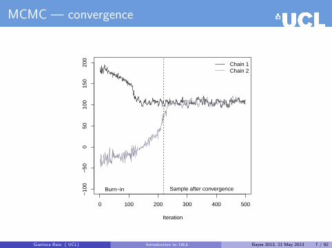
MCMC — convergence
0 100 200 300 400 500
−10
0−
500
5010
015
020
0
Iteration
Chain 1Chain 2
Burn−in Sample after convergence
Gianluca Baio ( UCL) Introduction to INLA Bayes 2013, 21 May 2013 7 / 92
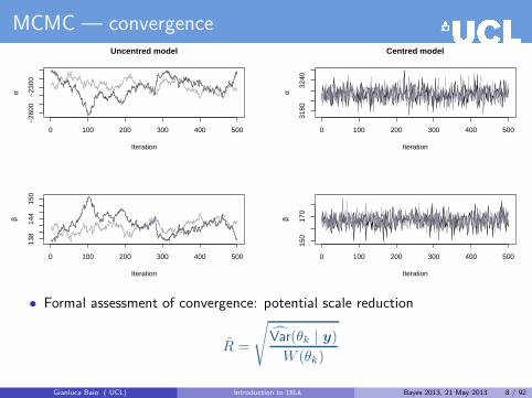
MCMC — convergence
0 100 200 300 400 500
−26
00−
2300
Uncentred model
Iteration
α
0 100 200 300 400 500
138
144
150
Iteration
β
0 100 200 300 400 500
3180
3240
Centred model
Iteration
α
0 100 200 300 400 500
150
170
Iteration
β
• Formal assessment of convergence: potential scale reduction
R =
√Var(θk | y)
W (θk)
Gianluca Baio ( UCL) Introduction to INLA Bayes 2013, 21 May 2013 8 / 92

MCMC — autocorrelation
0 5 10 15 20 25 30
0.0
0.2
0.4
0.6
0.8
1.0
Lag
Autocorrelation function for α − Uncentred model
0 5 10 15 20 25 30
0.0
0.2
0.4
0.6
0.8
1.0
Lag
Autocorrelation function for α − Centred model
• Formal assessment of autocorrelation: effective sample size
neff =S
1 + 2∑∞t=1 ρt
Gianluca Baio ( UCL) Introduction to INLA Bayes 2013, 21 May 2013 9 / 92

MCMC — brute force
0 100 200 300 400 500
−28
00−
2000
Uncentred model with thinning
Iteration
α
0 100 200 300 400 500
125
140
155
Iteration
β
0 5 10 15 20 25 300.
00.
20.
40.
60.
81.
0
Lag
Autocorrelation function for α − Uncentred model with thinning
Gianluca Baio ( UCL) Introduction to INLA Bayes 2013, 21 May 2013 10 / 92

MCMC — pros & cons
• “Standard” MCMC sampler are generally easy-ish to program and are in factimplemented in readily available software
• However, depending on the complexity of the problem, their efficiency mightbe limited
Gianluca Baio ( UCL) Introduction to INLA Bayes 2013, 21 May 2013 11 / 92

MCMC — pros & cons
• “Standard” MCMC sampler are generally easy-ish to program and are in factimplemented in readily available software
• However, depending on the complexity of the problem, their efficiency mightbe limited
• Possible solutions1 More complex model specification
• Blocking• Overparameterisation
2 More complex sampling schemes• Hamiltonian Monte Carlo• No U-turn sampling (eg stan — more on this later!)
3 Alternative methods of inference• Approximate Bayesian Computation (ABC)• INLA
Gianluca Baio ( UCL) Introduction to INLA Bayes 2013, 21 May 2013 11 / 92

Basics of INLA
The basic ideas revolve around
• Formulating the model using a specific characterisation
– All models that can be formulated in this way have certain features incommon, which facilitate the computational aspects
– The characterisation is still quite general and covers a wide range of possiblemodels (more on that later!)
– NB: This implies less flexibility with respect to MCMC — but in many casesthis is not a huge limitation!
Gianluca Baio ( UCL) Introduction to INLA Bayes 2013, 21 May 2013 12 / 92

Basics of INLA
The basic ideas revolve around
• Formulating the model using a specific characterisation
– All models that can be formulated in this way have certain features incommon, which facilitate the computational aspects
– The characterisation is still quite general and covers a wide range of possiblemodels (more on that later!)
– NB: This implies less flexibility with respect to MCMC — but in many casesthis is not a huge limitation!
• Use some basic probability conditions to approximate the relevantdistributions
• Compute the relevant quantities typically using numerical methods
Gianluca Baio ( UCL) Introduction to INLA Bayes 2013, 21 May 2013 12 / 92

Latent Gaussian models (LGMs)
• The general problem of (parametric) inference is posited by assuming aprobability model for the observed data, as a function of some relevantparameters
y | θ,ψ ∼ p(y | θ,ψ) =
n∏
i=1
p(yi | θ,ψ)
Gianluca Baio ( UCL) Introduction to INLA Bayes 2013, 21 May 2013 13 / 92

Latent Gaussian models (LGMs)
• The general problem of (parametric) inference is posited by assuming aprobability model for the observed data, as a function of some relevantparameters
y | θ,ψ ∼ p(y | θ,ψ) =
n∏
i=1
p(yi | θ,ψ)
• Often (in fact for a surprisingly large range of models!), we can assume thatthe parameters are described by a Gaussian Markov Random Field(GMRF)
θ | ψ ∼ Normal(0,Σ(ψ))
θl ⊥⊥ θm | θ−lm
where
– The notation “−lm” indicates all the other elements of the parameters vector,excluding elements l and m
– The covariance matrix Σ depends on some hyper-parameters ψ
• This kind of models is often referred to as Latent Gaussian models
Gianluca Baio ( UCL) Introduction to INLA Bayes 2013, 21 May 2013 13 / 92

LGMs as a general framework
• In general, we can partition ψ = (ψ1,ψ2) and re-express a LGM as
ψ ∼ p(ψ) (“hyperprior”)
θ | ψ ∼ p(θ | ψ) = Normal(0,Σ(ψ1)) (“GMRF prior”)
y | θ,ψ ∼∏
i
p(yi | θ,ψ2) (“data model”)
ie ψ1 are the hyper-parameters and ψ2 are nuisance parameters
Gianluca Baio ( UCL) Introduction to INLA Bayes 2013, 21 May 2013 14 / 92
LGMs as a general framework
• In general, we can partition ψ = (ψ1,ψ2) and re-express a LGM as
ψ ∼ p(ψ) (“hyperprior”)
θ | ψ ∼ p(θ | ψ) = Normal(0,Σ(ψ1)) (“GMRF prior”)
y | θ,ψ ∼∏
i
p(yi | θ,ψ2) (“data model”)
ie ψ1 are the hyper-parameters and ψ2 are nuisance parameters
• The dimension of θ can be very large (eg 102-105)
• Conversely, because of the conditional independence properties, thedimension of ψ is generally small (eg 1-5)
Gianluca Baio ( UCL) Introduction to INLA Bayes 2013, 21 May 2013 14 / 92

LGMs as a general framework
• A very general way of specifying the problem is by modelling the mean forthe i-th unit by means of an additive linear predictor, defined on a suitablescale (e.g. logistic for binomial data)
ηi = α+
M∑
m=1
βmxmi +
L∑
l=1
fl(zli)
where
– α is the intercept;– β = (β1, . . . , βM ) quantify the effect of x = (x1, . . . , xM ) on the response;– f = {f1(·), . . . , fL(·)} is a set of functions defined in terms of some covariatesz = (z1, . . . , zL)
and then assumeθ = (α,β,f) ∼ GMRF(ψ)
Gianluca Baio ( UCL) Introduction to INLA Bayes 2013, 21 May 2013 15 / 92

LGMs as a general framework
• A very general way of specifying the problem is by modelling the mean forthe i-th unit by means of an additive linear predictor, defined on a suitablescale (e.g. logistic for binomial data)
ηi = α+
M∑
m=1
βmxmi +
L∑
l=1
fl(zli)
where
– α is the intercept;– β = (β1, . . . , βM ) quantify the effect of x = (x1, . . . , xM ) on the response;– f = {f1(·), . . . , fL(·)} is a set of functions defined in terms of some covariatesz = (z1, . . . , zL)
and then assumeθ = (α,β,f) ∼ GMRF(ψ)
• NB: This of course implies some form of Normally-distributed marginals forα,β and f
Gianluca Baio ( UCL) Introduction to INLA Bayes 2013, 21 May 2013 15 / 92

LGMs as a general framework — examples
Upon varying the form of the functions fl(·), this formulation can accommodate awide range of models
Gianluca Baio ( UCL) Introduction to INLA Bayes 2013, 21 May 2013 16 / 92

LGMs as a general framework — examples
Upon varying the form of the functions fl(·), this formulation can accommodate awide range of models
• Standard regression
– fl(·) = NULL
Gianluca Baio ( UCL) Introduction to INLA Bayes 2013, 21 May 2013 16 / 92

LGMs as a general framework — examples
Upon varying the form of the functions fl(·), this formulation can accommodate awide range of models
• Standard regression
– fl(·) = NULL
• Hierarchical models
– fl(·) ∼ Normal(0, σ2f ) (Exchangeable)
σ2f | ψ ∼ some common distribution
• Spatial and spatio-temporal models
– Two components: f1(·) ∼ CAR (Spatially structured effects)Two components: f2(·) ∼ Normal(0, σ2
f2) (Unstructured residual)
• Spline smoothing
– fl(·) ∼ AR(φ, σ2ε)
• Survival models / logGaussian Cox Processes
– More complex specification in theory, but relatively easy to fit within the INLAframework!
Gianluca Baio ( UCL) Introduction to INLA Bayes 2013, 21 May 2013 16 / 92

Gaussian Markov Random Field
In order to preserve the underlying conditional independence structure in a GMRF,it is necessary to constrain the parameterisation
Gianluca Baio ( UCL) Introduction to INLA Bayes 2013, 21 May 2013 17 / 92

Gaussian Markov Random Field
In order to preserve the underlying conditional independence structure in a GMRF,it is necessary to constrain the parameterisation
• Generally, it is complicated to do it in terms of the covariance matrix Σ
– Typically, Σ is dense (ie many of the entries are non-zero)– If it happens to be sparse, this implies (marginal) independence among the
relevant elements of θ — this is generally too stringent a requirement!
• Conversely, it is much simpler when using the precision matrix Q =: Σ−1
– As it turns out, it can be shown that
θl ⊥⊥ θm | θ−lm ⇔ Qlm = 0
– Thus, under conditional independence (which is a less restrictive constraint),the precision matrix is typically sparse
– We can use existing numerical methods to deal with sparse matrices (eg the R
package Matrix)– Most computations in GMRFs are performed in terms of computing Cholesky’s
factorisations
Gianluca Baio ( UCL) Introduction to INLA Bayes 2013, 21 May 2013 17 / 92

Precision matrix and conditional independence
Gianluca Baio ( UCL) Introduction to INLA Bayes 2013, 21 May 2013 18 / 92

Precision matrix and conditional independence
Gianluca Baio ( UCL) Introduction to INLA Bayes 2013, 21 May 2013 18 / 92

Precision matrix and conditional independence
——————————————————–
Gianluca Baio ( UCL) Introduction to INLA Bayes 2013, 21 May 2013 18 / 92

MCMC and LGMs
• (Standard) MCMC methods tend to perform poorly when applied to(non-trivial) LGMs. This is due to several factors
– The components of the latent Gaussian field θ tend to be highly correlated,thus impacting on convergence and autocorrelation
– Especially when the number of observations is large, θ and ψ also tend to behighly correlated
ρ = 0.95 ρ = 0.20
θ1 θ1
θ2θ2
Gianluca Baio ( UCL) Introduction to INLA Bayes 2013, 21 May 2013 19 / 92

MCMC and LGMs
• (Standard) MCMC methods tend to perform poorly when applied to(non-trivial) LGMs. This is due to several factors
– The components of the latent Gaussian field θ tend to be highly correlated,thus impacting on convergence and autocorrelation
– Especially when the number of observations is large, θ and ψ also tend to behighly correlated
ρ = 0.95 ρ = 0.20
θ1 θ1
θ2θ2
• Again, blocking and overparameterisation can alleviate, but rarely eliminatethe problem
Gianluca Baio ( UCL) Introduction to INLA Bayes 2013, 21 May 2013 19 / 92

Summary so far
• Bayesian computation (especially for LGMs) is in general difficult
• MCMC can be efficiently used in many simple cases, but becomes a bittrickier for complex models
– Issues with convergence– Time to run can be very long
Gianluca Baio ( UCL) Introduction to INLA Bayes 2013, 21 May 2013 20 / 92

Summary so far
• Bayesian computation (especially for LGMs) is in general difficult
• MCMC can be efficiently used in many simple cases, but becomes a bittrickier for complex models
– Issues with convergence– Time to run can be very long
• A wide class of statistical models can be represented in terms of LGM
• This allows us to take advantage of nice computational properties
– GMRFs– Sparse precision matrices
• This is at the heart of the INLA approach
Gianluca Baio ( UCL) Introduction to INLA Bayes 2013, 21 May 2013 20 / 92

Introduction to INLA
Gianluca Baio ( UCL) Introduction to INLA Bayes 2013, 21 May 2013 21 / 92

Integrated Nested Laplace Approximation (INLA)
• The starting point to understand the INLA approach is the definition ofconditional probability, which holds for any pair of variables (x, z) — and,technically, provided p(z) > 0
p(x | z) =:p(x, z)
p(z)
which can be re-written as
p(z) =p(x, z)
p(x | z)
Gianluca Baio ( UCL) Introduction to INLA Bayes 2013, 21 May 2013 22 / 92

Integrated Nested Laplace Approximation (INLA)
• The starting point to understand the INLA approach is the definition ofconditional probability, which holds for any pair of variables (x, z) — and,technically, provided p(z) > 0
p(x | z) =:p(x, z)
p(z)
which can be re-written as
p(z) =p(x, z)
p(x | z)
• In particular, a conditional version can be obtained further considering a thirdvariable w as
p(z | w) =p(x, z | w)
p(x | z, w)
which is particularly relevant to the Bayesian case
Gianluca Baio ( UCL) Introduction to INLA Bayes 2013, 21 May 2013 22 / 92

Integrated Nested Laplace Approximation (INLA)
• The second “ingredient” is Laplace approximation
Gianluca Baio ( UCL) Introduction to INLA Bayes 2013, 21 May 2013 23 / 92

Integrated Nested Laplace Approximation (INLA)
• The second “ingredient” is Laplace approximation
• Main idea: approximate log g(x) using a quadratic function by means of aTaylor’s series expansion around the mode x
log g(x) ≈ log g(x) +∂ log g(x)
∂x(x− x) +
1
2
∂2 log g(x)
∂x2(x− x)2
= log g(x) +1
2
∂2 log g(x)
∂x2(x − x)2
(since ∂ log g(x)
∂x= 0
)
• Setting σ2 = −1/∂2 log g(x)
∂x2 we can re-write
log g(x) ≈ log g(x)−1
2σ2(x− x)2
or equivalently∫g(x)dx =
∫elog g(x)dx ≈ const
∫exp
[−(x− x)2
2σ2
]dx
• Thus, under LA, g(x) ≈ Normal(x, σ2)
Gianluca Baio ( UCL) Introduction to INLA Bayes 2013, 21 May 2013 23 / 92

Laplace approximation — example
• Consider a χ2 distribution: p(x) =g(x)
c=xk2−1e
−x2
c
Gianluca Baio ( UCL) Introduction to INLA Bayes 2013, 21 May 2013 24 / 92

Laplace approximation — example
• Consider a χ2 distribution: p(x) =g(x)
c=xk2−1e
−x2
c
1 l(x) = log g(x) =
(
k
2− 1
)
log x−x
2
Gianluca Baio ( UCL) Introduction to INLA Bayes 2013, 21 May 2013 24 / 92

Laplace approximation — example
• Consider a χ2 distribution: p(x) =g(x)
c=xk2−1e
−x2
c
1 l(x) = log g(x) =
(
k
2− 1
)
log x−x
2
2 l′(x) =
∂ log g(x)
∂x=
(
k
2− 1
)
x−1 −
1
2
Gianluca Baio ( UCL) Introduction to INLA Bayes 2013, 21 May 2013 24 / 92

Laplace approximation — example
• Consider a χ2 distribution: p(x) =g(x)
c=xk2−1e
−x2
c
1 l(x) = log g(x) =
(
k
2− 1
)
log x−x
2
2 l′(x) =
∂ log g(x)
∂x=
(
k
2− 1
)
x−1 −
1
2
3 l′′(x) =
∂2 log g(x)
∂x2= −
(
k
2− 1
)
x−2
Gianluca Baio ( UCL) Introduction to INLA Bayes 2013, 21 May 2013 24 / 92

Laplace approximation — example
• Consider a χ2 distribution: p(x) =g(x)
c=xk2−1e
−x2
c
1 l(x) = log g(x) =
(
k
2− 1
)
log x−x
2
2 l′(x) =
∂ log g(x)
∂x=
(
k
2− 1
)
x−1 −
1
2
3 l′′(x) =
∂2 log g(x)
∂x2= −
(
k
2− 1
)
x−2
• Then
– Solving l′(x) = 0 we find the mode: x = k − 2
– Evaluating −1
l′′(x)at the mode gives σ2 = 2(k − 2)
Gianluca Baio ( UCL) Introduction to INLA Bayes 2013, 21 May 2013 24 / 92
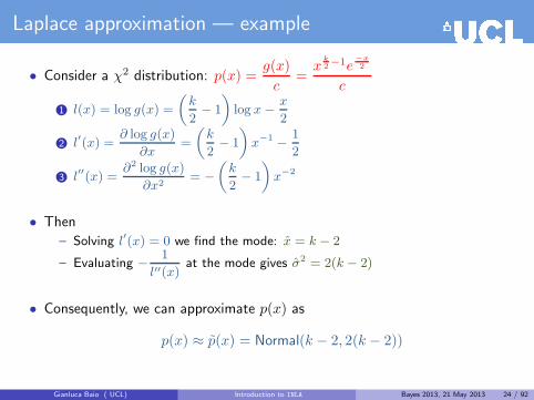
Laplace approximation — example
• Consider a χ2 distribution: p(x) =g(x)
c=xk2−1e
−x2
c
1 l(x) = log g(x) =
(
k
2− 1
)
log x−x
2
2 l′(x) =
∂ log g(x)
∂x=
(
k
2− 1
)
x−1 −
1
2
3 l′′(x) =
∂2 log g(x)
∂x2= −
(
k
2− 1
)
x−2
• Then
– Solving l′(x) = 0 we find the mode: x = k − 2
– Evaluating −1
l′′(x)at the mode gives σ2 = 2(k − 2)
• Consequently, we can approximate p(x) as
p(x) ≈ p(x) = Normal(k − 2, 2(k − 2))
Gianluca Baio ( UCL) Introduction to INLA Bayes 2013, 21 May 2013 24 / 92

Laplace approximation — example
0 2 4 6 8 10
0.00
0.05
0.10
0.15
0.20
0.25
0.30
0 5 10 15
0.00
0.05
0.10
0.15
0 5 10 15 20
0.00
0.02
0.04
0.06
0.08
0.10
0 10 20 30 40
0.00
0.02
0.04
0.06
— χ2(3)
- - - Normal(1, 2)
— χ2(6)
- - - Normal(4, 8)
— χ2(10)
- - - Normal(8, 16)
— χ2(20)
- - - Normal(18, 36)
Gianluca Baio ( UCL) Introduction to INLA Bayes 2013, 21 May 2013 25 / 92

Integrated Nested Laplace Approximation (INLA)
• The general idea is that using the fundamental probability equations, we canapproximate a generic conditional (posterior) distribution as
p(z | w) =p(x, z | w)
p(x | z, w),
where p(x | z, w) is the Laplace approximation to the conditional distributionof x given z, w
Gianluca Baio ( UCL) Introduction to INLA Bayes 2013, 21 May 2013 26 / 92

Integrated Nested Laplace Approximation (INLA)
• The general idea is that using the fundamental probability equations, we canapproximate a generic conditional (posterior) distribution as
p(z | w) =p(x, z | w)
p(x | z, w),
where p(x | z, w) is the Laplace approximation to the conditional distributionof x given z, w
• This idea can be used to approximate any generic required posteriordistribution
Gianluca Baio ( UCL) Introduction to INLA Bayes 2013, 21 May 2013 26 / 92

Integrated Nested Laplace Approximation (INLA)
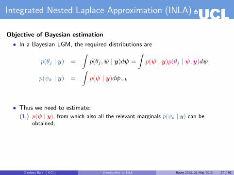
Objective of Bayesian estimation
• In a Bayesian LGM, the required distributions are
p(θj | y) =
∫p(θj ,ψ | y)dψ =
∫p(ψ | y)p(θj | ψ,y)dψ
p(ψk | y) =
∫p(ψ | y)dψ−k
Gianluca Baio ( UCL) Introduction to INLA Bayes 2013, 21 May 2013 27 / 92
Integrated Nested Laplace Approximation (INLA)
Objective of Bayesian estimation
• In a Bayesian LGM, the required distributions are
p(θj | y) =
∫p(θj ,ψ | y)dψ =
∫p(ψ | y)p(θj | ψ,y)dψ
p(ψk | y) =
∫p(ψ | y)dψ−k
• Thus we need to estimate:
(1.) p(ψ | y), from which also all the relevant marginals p(ψk | y) can beobtained;
Gianluca Baio ( UCL) Introduction to INLA Bayes 2013, 21 May 2013 27 / 92

Integrated Nested Laplace Approximation (INLA)
Objective of Bayesian estimation
• In a Bayesian LGM, the required distributions are
p(θj | y) =
∫p(θj ,ψ | y)dψ =
∫p(ψ | y)p(θj | ψ,y)dψ
p(ψk | y) =
∫p(ψ | y)dψ−k
• Thus we need to estimate:
(1.) p(ψ | y), from which also all the relevant marginals p(ψk | y) can beobtained;
(2.) p(θj | ψ,y), which is needed to compute the marginal posterior for theparameters
Gianluca Baio ( UCL) Introduction to INLA Bayes 2013, 21 May 2013 27 / 92
Integrated Nested Laplace Approximation (INLA)
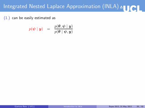
(1.) can be easily estimated as
p(ψ | y) =p(θ,ψ | y)
p(θ | ψ,y)
Gianluca Baio ( UCL) Introduction to INLA Bayes 2013, 21 May 2013 28 / 92

Integrated Nested Laplace Approximation (INLA)
(1.) can be easily estimated as
p(ψ | y) =p(θ,ψ | y)
p(θ | ψ,y)
=p(y | θ,ψ)p(θ,ψ)
p(y)
1
p(θ | ψ,y)
Gianluca Baio ( UCL) Introduction to INLA Bayes 2013, 21 May 2013 28 / 92

Integrated Nested Laplace Approximation (INLA)
(1.) can be easily estimated as
p(ψ | y) =p(θ,ψ | y)
p(θ | ψ,y)
=p(y | θ,ψ)p(θ,ψ)
p(y)
1
p(θ | ψ,y)
=p(y | θ)p(θ | ψ)p(ψ)
p(y)
1
p(θ | ψ,y)
Gianluca Baio ( UCL) Introduction to INLA Bayes 2013, 21 May 2013 28 / 92

Integrated Nested Laplace Approximation (INLA)
(1.) can be easily estimated as
p(ψ | y) =p(θ,ψ | y)
p(θ | ψ,y)
=p(y | θ,ψ)p(θ,ψ)
p(y)
1
p(θ | ψ,y)
=p(y | θ)p(θ | ψ)p(ψ)
p(y)
1
p(θ | ψ,y)
∝p(ψ)p(θ | ψ)p(y | θ)
p(θ | ψ,y)
Gianluca Baio ( UCL) Introduction to INLA Bayes 2013, 21 May 2013 28 / 92

Integrated Nested Laplace Approximation (INLA)
(1.) can be easily estimated as
p(ψ | y) =p(θ,ψ | y)
p(θ | ψ,y)
=p(y | θ,ψ)p(θ,ψ)
p(y)
1
p(θ | ψ,y)
=p(y | θ)p(θ | ψ)p(ψ)
p(y)
1
p(θ | ψ,y)
∝p(ψ)p(θ | ψ)p(y | θ)
p(θ | ψ,y)
≈p(ψ)p(θ | ψ)p(y | θ)
p(θ | ψ,y)
∣∣∣∣θ=θ(ψ)
=: p(ψ | y)
where
– p(θ | ψ,y) is the Laplace approximation of p(θ | ψ,y)– θ = θ(ψ) is its mode
Gianluca Baio ( UCL) Introduction to INLA Bayes 2013, 21 May 2013 28 / 92

Integrated Nested Laplace Approximation (INLA)
(2.) is slightly more complex, because in general there will be more elements in θthan there are in ψ and thus this computation is more expensive
Gianluca Baio ( UCL) Introduction to INLA Bayes 2013, 21 May 2013 29 / 92

Integrated Nested Laplace Approximation (INLA)
(2.) is slightly more complex, because in general there will be more elements in θthan there are in ψ and thus this computation is more expensive
• One easy possibility is to approximate p(θj | ψ,y) directly using a Normaldistribution, where the precision matrix is based on the Choleskydecomposition of the precision matrix Q. While this is very fast, theapproximation is generally not very good
• Alternatively, we can write θ = {θj , θ−j}, use the definition of conditionalprobability and again Laplace approximation to obtain
p(θj | ψ,y) =p ({θj , θ−j} | ψ,y)
p(θ−j | θj ,ψ,y)
Gianluca Baio ( UCL) Introduction to INLA Bayes 2013, 21 May 2013 29 / 92

Integrated Nested Laplace Approximation (INLA)
(2.) is slightly more complex, because in general there will be more elements in θthan there are in ψ and thus this computation is more expensive
• One easy possibility is to approximate p(θj | ψ,y) directly using a Normaldistribution, where the precision matrix is based on the Choleskydecomposition of the precision matrix Q. While this is very fast, theapproximation is generally not very good
• Alternatively, we can write θ = {θj , θ−j}, use the definition of conditionalprobability and again Laplace approximation to obtain
p(θj | ψ,y) =p ({θj , θ−j} | ψ,y)
p(θ−j | θj ,ψ,y)=p ({θj , θ−j},ψ | y)
p(ψ | y)
1
p(θ−j | θj ,ψ,y)
∝p (θ,ψ | y)
p(θ−j | θj ,ψ,y)
Gianluca Baio ( UCL) Introduction to INLA Bayes 2013, 21 May 2013 29 / 92

Integrated Nested Laplace Approximation (INLA)
(2.) is slightly more complex, because in general there will be more elements in θthan there are in ψ and thus this computation is more expensive
• One easy possibility is to approximate p(θj | ψ,y) directly using a Normaldistribution, where the precision matrix is based on the Choleskydecomposition of the precision matrix Q. While this is very fast, theapproximation is generally not very good
• Alternatively, we can write θ = {θj , θ−j}, use the definition of conditionalprobability and again Laplace approximation to obtain
p(θj | ψ,y) =p ({θj , θ−j} | ψ,y)
p(θ−j | θj ,ψ,y)=p ({θj , θ−j},ψ | y)
p(ψ | y)
1
p(θ−j | θj ,ψ,y)
∝p (θ,ψ | y)
p(θ−j | θj ,ψ,y)∝p(ψ)p(θ | ψ)p(y | θ)
p(θ−j | θj ,ψ,y)
≈p(ψ)p(θ | ψ)p(y | θ)
p(θ−j | θj ,ψ,y)
∣∣∣∣θ−j=θ−j(θj,ψ)
=: p(θj | ψ,y)
Gianluca Baio ( UCL) Introduction to INLA Bayes 2013, 21 May 2013 29 / 92

Integrated Nested Laplace Approximation (INLA)
• Because (θ−j | θj ,ψ,y) are reasonably Normal, the approximation worksgenerally well
• However, this strategy can be computationally expensive
Gianluca Baio ( UCL) Introduction to INLA Bayes 2013, 21 May 2013 30 / 92

Integrated Nested Laplace Approximation (INLA)
• Because (θ−j | θj ,ψ,y) are reasonably Normal, the approximation worksgenerally well
• However, this strategy can be computationally expensive
• The most efficient algorithm is the “Simplified Laplace Approximation”
– Based on a Taylor’s series expansion up to the third order of both numeratorand denominator for p(θj | ψ,y)
– This effectively “corrects” the Gaussian approximation for location andskewness to increase the fit to the required distribution
• This is the algorithm implemented by default by R-INLA, but this choice canbe modified
– If extra precision is required, it is possible to run the full Laplaceapproximation — of course at the expense of running time!
Gianluca Baio ( UCL) Introduction to INLA Bayes 2013, 21 May 2013 30 / 92

Integrated Nested Laplace Approximation (INLA)
Operationally, the INLA algorithm proceeds with the following steps:i. Explore the marginal joint posterior for the hyper-parameters p(ψ | y)
ψ1
ψ2
Gianluca Baio ( UCL) Introduction to INLA Bayes 2013, 21 May 2013 31 / 92

Integrated Nested Laplace Approximation (INLA)
Operationally, the INLA algorithm proceeds with the following steps:i. Explore the marginal joint posterior for the hyper-parameters p(ψ | y)
– Locate the mode ψ by optimising log p(ψ | y), eg using Newton-likealgorithms
– Compute the Hessian at ψ and change co-ordinates to standardise thevariables; this corrects for scale and rotation and simplifies integration
ψ1
ψ2
z 1z 2
E[z] = 0
V[z] = σ2I
Gianluca Baio ( UCL) Introduction to INLA Bayes 2013, 21 May 2013 31 / 92

Integrated Nested Laplace Approximation (INLA)
Operationally, the INLA algorithm proceeds with the following steps:i. Explore the marginal joint posterior for the hyper-parameters p(ψ | y)
– Locate the mode ψ by optimising log p(ψ | y), eg using Newton-likealgorithms
– Compute the Hessian at ψ and change co-ordinates to standardise thevariables; this corrects for scale and rotation and simplifies integration
– Explore log p(ψ | y) and produce a grid of H points {ψ∗
h} associated with thebulk of the mass, together with a corresponding set of area weights {∆h}
ψ1
ψ2
z 1z 2
Gianluca Baio ( UCL) Introduction to INLA Bayes 2013, 21 May 2013 31 / 92
Integrated Nested Laplace Approximation (INLA)
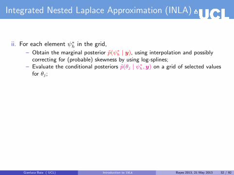
ii. For each element ψ∗h in the grid,
– Obtain the marginal posterior p(ψ∗
h | y), using interpolation and possiblycorrecting for (probable) skewness by using log-splines;
– Evaluate the conditional posteriors p(θj | ψ∗
h,y) on a grid of selected valuesfor θj ;
Gianluca Baio ( UCL) Introduction to INLA Bayes 2013, 21 May 2013 32 / 92

Integrated Nested Laplace Approximation (INLA)
ii. For each element ψ∗h in the grid,
– Obtain the marginal posterior p(ψ∗
h | y), using interpolation and possiblycorrecting for (probable) skewness by using log-splines;
– Evaluate the conditional posteriors p(θj | ψ∗
h,y) on a grid of selected valuesfor θj ;
iii. Marginalise ψ∗h to obtain the marginal posteriors p(θj | y) using numerical
integration
p(θj | y) ≈
H∑
h=1
p(θj | ψ∗h,y)p(ψ
∗h | y)∆h
Gianluca Baio ( UCL) Introduction to INLA Bayes 2013, 21 May 2013 32 / 92

Integrated Nested Laplace Approximation (INLA)
So, it’s all in the name...
Integrated Nested Laplace Approximation
• Because Laplace approximation is the basis to estimate the unknowndistributions
• Because the Laplace approximations are nested within one another
– Since (2.) is needed to estimate (1.)– NB: Consequently the estimation of (1.) might not be good enough, but it
can be refined
• Because the required marginal posterior distributions are obtained by(numerical) integration
Gianluca Baio ( UCL) Introduction to INLA Bayes 2013, 21 May 2013 33 / 92

INLA — example
• Suppose we want to make inference on a very simple model
yij | θj , ψ ∼ Normal(θj , σ20) (σ2
0 assumed known)
θj | ψ ∼ Normal(0, τ) (ψ = τ−1 is the precision)
ψ ∼ Gamma(a, b)
Gianluca Baio ( UCL) Introduction to INLA Bayes 2013, 21 May 2013 34 / 92

INLA — example
• Suppose we want to make inference on a very simple model
yij | θj , ψ ∼ Normal(θj , σ20) (σ2
0 assumed known)
θj | ψ ∼ Normal(0, τ) (ψ = τ−1 is the precision)
ψ ∼ Gamma(a, b)
• So, the model is made by a three-level hierarchy:
1 Data y = (yij) for i = 1, . . . , nj and j = 1, . . . , J2 Parameters θ = (θ1, . . . , θJ )3 Hyper-parameter ψ
• NB: This model is in fact semi-conjugated, so inference is possiblenumerically or using simple MCMC algorithms
Gianluca Baio ( UCL) Introduction to INLA Bayes 2013, 21 May 2013 34 / 92

INLA — example
• Because of semi-conjugacy, we know that
θ,y | ψ ∼ Normal(·, ·)
and thus we can compute (numerically) all the marginals
Gianluca Baio ( UCL) Introduction to INLA Bayes 2013, 21 May 2013 35 / 92

INLA — example
• Because of semi-conjugacy, we know that
θ,y | ψ ∼ Normal(·, ·)
and thus we can compute (numerically) all the marginals
• In particular
p(ψ | y) ∝ p(y | ψ)p(ψ)
∝
Gaussian︷ ︸︸ ︷p(θ,y | ψ) p(ψ)
p(θ | y, ψ)︸ ︷︷ ︸Gaussian
• Moreover, because p(θ | y) ∼ Normal(·, ·) and so are all the resultingmarginals (ie for every element j), it is easy to compute
p(θj | y) =
∫p(θj | y, ψ)︸ ︷︷ ︸
Gaussian
p(ψ | y)︸ ︷︷ ︸Approximated
dψ
Gianluca Baio ( UCL) Introduction to INLA Bayes 2013, 21 May 2013 35 / 92

INLA — example
1. Select a grid of H points for ψ ({ψ∗
h}) and the associated area weights ({∆h})
Posterior marginal for ψ : p(ψ | y) ∝ p(θ,y|ψ)p(ψ)p(θ|y,ψ)
1 2 3 4 5 6
0.0
0.2
0.4
0.6
0.8
1.0
Log precision
Exp
onen
tial o
f log
den
sity
Gianluca Baio ( UCL) Introduction to INLA Bayes 2013, 21 May 2013 36 / 92

INLA — example
2. Interpolate the posterior density to compute the approximation to the posterior
Posterior marginal for ψ (interpolated)
1 2 3 4 5 6
0.0
0.2
0.4
0.6
0.8
1.0
Log precision
Exp
onen
tial o
f log
den
sity
Gianluca Baio ( UCL) Introduction to INLA Bayes 2013, 21 May 2013 37 / 92

INLA — example
3. Compute the posterior marginal for each θj given each ψ on the H−dimensional grid
Posterior marginal for θ1, conditional on each {ψ∗h} value (unweighted)
−14 −12 −10 −8
0.0
0.2
0.4
0.6
0.8
1.0
Den
sity
θ1
Gianluca Baio ( UCL) Introduction to INLA Bayes 2013, 21 May 2013 38 / 92

INLA — example
4. Weight the resulting (conditional) marginal posteriors by the density associated with eachψ on the grid
Posterior marginal for θ1, conditional on each {ψ∗h} value (weighted)
−14 −12 −10 −8
0.00
0.02
0.04
0.06
0.08
Den
sity
θ1
Gianluca Baio ( UCL) Introduction to INLA Bayes 2013, 21 May 2013 39 / 92

INLA — example
5. (Numerically) sum over all the conditional densities to obtain the marginal posterior foreach of the elements θj
Posterior marginal for θ1 : p(θ1 | y)
−14 −12 −10 −8
0.0
0.1
0.2
0.3
0.4
0.5
Den
sity
θ1
Gianluca Baio ( UCL) Introduction to INLA Bayes 2013, 21 May 2013 40 / 92

INLA — Summary
• The basic idea behind the INLA procedure is simple
– Repeatedly use Laplace approximation and take advantage of computationalsimplifications due to the structure of the model
– Use numerical integration to compute the required posterior marginaldistributions
– (If necessary) refine the estimation (eg using a finer grid)
Gianluca Baio ( UCL) Introduction to INLA Bayes 2013, 21 May 2013 41 / 92

INLA — Summary
• The basic idea behind the INLA procedure is simple
– Repeatedly use Laplace approximation and take advantage of computationalsimplifications due to the structure of the model
– Use numerical integration to compute the required posterior marginaldistributions
– (If necessary) refine the estimation (eg using a finer grid)
• Complications are mostly computational and occur when
– Extending to more than one hyper-parameter– Markedly non-Gaussian observations
Gianluca Baio ( UCL) Introduction to INLA Bayes 2013, 21 May 2013 41 / 92

Using the package R-INLA
Gianluca Baio ( UCL) Introduction to INLA Bayes 2013, 21 May 2013 42 / 92

The INLA package for R
Good news is that all the procedures needed to perform INLA are implemented ina R package. This is effectively made by two components
Gianluca Baio ( UCL) Introduction to INLA Bayes 2013, 21 May 2013 43 / 92

The INLA package for R
Good news is that all the procedures needed to perform INLA are implemented ina R package. This is effectively made by two components
1 The GMRFLib library– This is a C library for fast and exact simulation of GMRFs, used to perform
• Unconditional simulation of a GMRF;• Various types of conditional simulation from a GMRF;• Evaluation of the corresponding log-density;• Generation of blockupdates in MCMC-algorithms using GMRF-approximations
or auxilliary variables, construction of non-Gaussian approximations to hiddenGMRFs, approximate inference using INLA
2 The inla program– A standalone C program that
• Interfaces with GMRFLib• Performs the relevant computation and returns the results in a standardised way
NB: Because the package R-INLA relies on a standalone C program, it is notavailable directly from CRAN
Gianluca Baio ( UCL) Introduction to INLA Bayes 2013, 21 May 2013 43 / 92

The INLA package for R — Installation
• Visit the websitewww.r-inla.org
and follow the instructions
• The website contains source code, examples, papers and reports discussingthe theory and applications of INLA
Gianluca Baio ( UCL) Introduction to INLA Bayes 2013, 21 May 2013 44 / 92

The INLA package for R — Installation
• Visit the websitewww.r-inla.org
and follow the instructions
• The website contains source code, examples, papers and reports discussingthe theory and applications of INLA
• From R, installation is performed typingsource("http://www.math.ntnu.no/inla/givemeINLA.R")
• Later, you can upgrade the package by typinginla.upgrade()
• A test-version (which may contain unstable updates/new functions) can beobtained by typinginla.upgrade(testing=TRUE)
• R-INLA runs natively under Linux, Windows and Mac and it is possible to domulti-threading using OpenMP
Gianluca Baio ( UCL) Introduction to INLA Bayes 2013, 21 May 2013 44 / 92
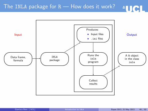
The INLA package for R — How does it work?
Input
Produces:
• Input files
• .ini files
Output
Data frame,formula
INLApackage
Runs theinla
program
A R objectin the class
inla
Collectresults
Gianluca Baio ( UCL) Introduction to INLA Bayes 2013, 21 May 2013 45 / 92

The INLA package for R — Documentation
• There has been a great effort lately in producing quite a lot user-frienly(-ish)documentation
• Tutorials are (or will shortly be) available on
– Basic INLA (probably later this year)– SPDE (spatial models based on stochastic partial differential equations)
models
Gianluca Baio ( UCL) Introduction to INLA Bayes 2013, 21 May 2013 46 / 92

The INLA package for R — Documentation
• There has been a great effort lately in producing quite a lot user-frienly(-ish)documentation
• Tutorials are (or will shortly be) available on
– Basic INLA (probably later this year)– SPDE (spatial models based on stochastic partial differential equations)
models
• Much of the recent development in R-INLA is devoted to extending theapplications of INLA for spatial and spatio-temporal models as well asproducing detailed information
• The website also has a discussion forum and a FAQ page
Gianluca Baio ( UCL) Introduction to INLA Bayes 2013, 21 May 2013 46 / 92

Step by step guide to using R-INLA
1. The first thing to do is to specify the model
• For example, assume we have a generic model
yiiid∼ p(yi | θi)
ηi = g(θi) = β0 + β1x1i + β2x2i + f(zi)
where
– x = (x1, x2) are observed covariates for which we are assuming a linear effecton some function g(·) of the parameter θi
– β = (β0, β1, β2) ∼ Normal(0, τ−11 ) are unstructured (“fixed”) effects
– z is an index. This can be used to include structured (“random”), spatial,spatio-temporal effect, etc.
– f ∼ Normal(0,Q−1f (τ2)) is a suitable function used to model the structured
effects
Gianluca Baio ( UCL) Introduction to INLA Bayes 2013, 21 May 2013 47 / 92

Step by step guide to using R-INLA
1. The first thing to do is to specify the model
• For example, assume we have a generic model
yiiid∼ p(yi | θi)
ηi = g(θi) = β0 + β1x1i + β2x2i + f(zi)
where
– x = (x1, x2) are observed covariates for which we are assuming a linear effecton some function g(·) of the parameter θi
– β = (β0, β1, β2) ∼ Normal(0, τ−11 ) are unstructured (“fixed”) effects
– z is an index. This can be used to include structured (“random”), spatial,spatio-temporal effect, etc.
– f ∼ Normal(0,Q−1f (τ2)) is a suitable function used to model the structured
effects
• As mentioned earlier, this formulation can actually be used to represent quitea wide class of models!
Gianluca Baio ( UCL) Introduction to INLA Bayes 2013, 21 May 2013 47 / 92
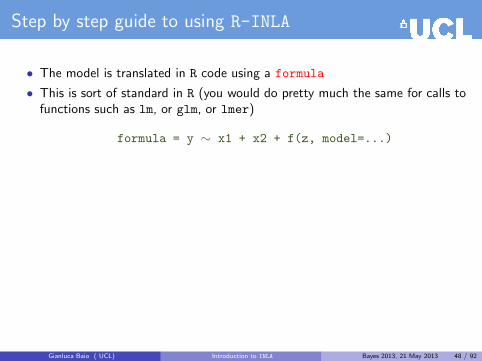
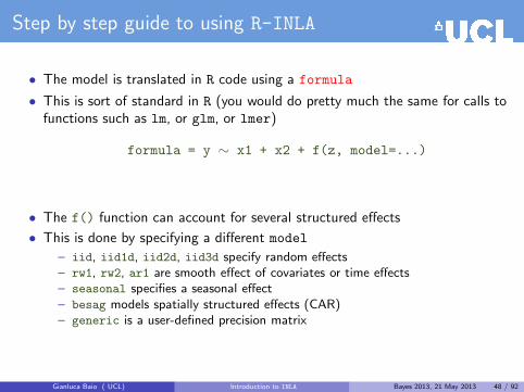
Step by step guide to using R-INLA
• The model is translated in R code using a formula
• This is sort of standard in R (you would do pretty much the same for calls tofunctions such as lm, or glm, or lmer)
formula = y ∼ x1 + x2 + f(z, model=...)
Gianluca Baio ( UCL) Introduction to INLA Bayes 2013, 21 May 2013 48 / 92
Step by step guide to using R-INLA
• The model is translated in R code using a formula
• This is sort of standard in R (you would do pretty much the same for calls tofunctions such as lm, or glm, or lmer)
formula = y ∼ x1 + x2 + f(z, model=...)
• The f() function can account for several structured effects
• This is done by specifying a different model
– iid, iid1d, iid2d, iid3d specify random effects– rw1, rw2, ar1 are smooth effect of covariates or time effects– seasonal specifies a seasonal effect– besag models spatially structured effects (CAR)– generic is a user-defined precision matrix
Gianluca Baio ( UCL) Introduction to INLA Bayes 2013, 21 May 2013 48 / 92

Step by step guide to using R-INLA
2. Call the function inla, specifying the data and options (more on this later),eg
m = inla(formula, data=data.frame(y,x1,x2,z))
Gianluca Baio ( UCL) Introduction to INLA Bayes 2013, 21 May 2013 49 / 92

Step by step guide to using R-INLA
2. Call the function inla, specifying the data and options (more on this later),eg
m = inla(formula, data=data.frame(y,x1,x2,z))
• The data need to be included in a suitable data.frame
• R returns an object m in the class inla, which has some methods available
– summary()
– plot()
• The options let you specify the priors and hyperpriors, together withadditional output
Gianluca Baio ( UCL) Introduction to INLA Bayes 2013, 21 May 2013 49 / 92
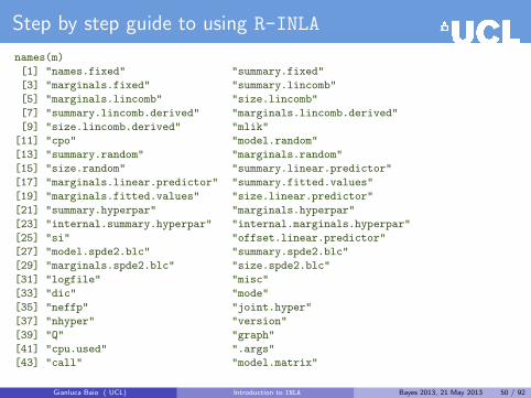
Step by step guide to using R-INLA
names(m)
[1] "names.fixed" "summary.fixed"
[3] "marginals.fixed" "summary.lincomb"
[5] "marginals.lincomb" "size.lincomb"
[7] "summary.lincomb.derived" "marginals.lincomb.derived"
[9] "size.lincomb.derived" "mlik"
[11] "cpo" "model.random"
[13] "summary.random" "marginals.random"
[15] "size.random" "summary.linear.predictor"
[17] "marginals.linear.predictor" "summary.fitted.values"
[19] "marginals.fitted.values" "size.linear.predictor"
[21] "summary.hyperpar" "marginals.hyperpar"
[23] "internal.summary.hyperpar" "internal.marginals.hyperpar"
[25] "si" "offset.linear.predictor"
[27] "model.spde2.blc" "summary.spde2.blc"
[29] "marginals.spde2.blc" "size.spde2.blc"
[31] "logfile" "misc"
[33] "dic" "mode"
[35] "neffp" "joint.hyper"
[37] "nhyper" "version"
[39] "Q" "graph"
[41] "cpu.used" ".args"
[43] "call" "model.matrix"
Gianluca Baio ( UCL) Introduction to INLA Bayes 2013, 21 May 2013 50 / 92

Example — Binary data with individual random effect
First, generate some data from an assumed model
yi ∼ Binomial(πi, Ni), for i = 1, . . . , n = 12
library(INLA)
# Data generationn=12Ntrials = sample(c(80:100), size=n, replace=TRUE)eta = rnorm(n,0,0.5)prob = exp(eta)/(1 + exp(eta))y = rbinom(n, size=Ntrials, prob = prob)data=data.frame(y=y,z=1:n,Ntrials)
Gianluca Baio ( UCL) Introduction to INLA Bayes 2013, 21 May 2013 51 / 92

Example — Binary data with individual random effect
data
y z Ntrials1 50 1 952 37 2 973 36 3 934 47 4 965 39 5 806 67 6 977 60 7 898 57 8 849 34 9 8910 57 10 9611 46 11 8712 48 12 98
Gianluca Baio ( UCL) Introduction to INLA Bayes 2013, 21 May 2013 52 / 92

Example — Binary data with individual random effect
data
y z Ntrials1 50 1 952 37 2 973 36 3 934 47 4 965 39 5 806 67 6 977 60 7 898 57 8 849 34 9 8910 57 10 9611 46 11 8712 48 12 98
We want to fit the following model
yi ∼ Binomial(πi, Ni), for i = 1, . . . , n = 12
logit(πi) = α+ f(zi)
α ∼ Normal(0, 1 000) (“fixed” effect)
f(zi) ∼ Normal(0, σ2) (“random” effect)
p(σ2) ∝ σ−2 = τ (“non-informative” prior)
≈ log σ ∼ Uniform(0,∞)
This can be done by typing in R
formula = y ∼ f(z,model="iid",hyper=list(list(prior="flat")))
m=inla(formula, data=data,family="binomial",Ntrials=Ntrials,control.predictor = list(compute = TRUE))
summary(m)
Gianluca Baio ( UCL) Introduction to INLA Bayes 2013, 21 May 2013 52 / 92
Example — Binary data with individual random effect
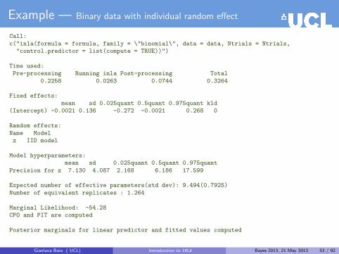
Call:
c("inla(formula = formula, family = \"binomial\", data = data, Ntrials = Ntrials,"control.predictor = list(compute = TRUE))")
Time used:Pre-processing Running inla Post-processing Total
0.2258 0.0263 0.0744 0.3264
Fixed effects:
mean sd 0.025quant 0.5quant 0.975quant kld(Intercept) -0.0021 0.136 -0.272 -0.0021 0.268 0
Random effects:
Name Modelz IID model
Model hyperparameters:mean sd 0.025quant 0.5quant 0.975quant
Precision for z 7.130 4.087 2.168 6.186 17.599
Expected number of effective parameters(std dev): 9.494(0.7925)
Number of equivalent replicates : 1.264
Marginal Likelihood: -54.28CPO and PIT are computed
Posterior marginals for linear predictor and fitted values computed
Gianluca Baio ( UCL) Introduction to INLA Bayes 2013, 21 May 2013 53 / 92

Exploring the R-INLA output
Fixed effects:mean sd 0.025quant 0.5quant 0.975quant kld
(Intercept) -0.0021 0.136 -0.272 -0.0021 0.268 0
Gianluca Baio ( UCL) Introduction to INLA Bayes 2013, 21 May 2013 54 / 92

Exploring the R-INLA output
Fixed effects:mean sd 0.025quant 0.5quant 0.975quant kld
(Intercept) -0.0021 0.136 -0.272 -0.0021 0.268 0
• For each unstructured (“fixed”) effect, R-INLA reports a set of summarystatistics from the posterior distribution
Gianluca Baio ( UCL) Introduction to INLA Bayes 2013, 21 May 2013 54 / 92
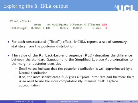
Exploring the R-INLA output
Fixed effects:mean sd 0.025quant 0.5quant 0.975quant kld
(Intercept) -0.0021 0.136 -0.272 -0.0021 0.268 0
• For each unstructured (“fixed”) effect, R-INLA reports a set of summarystatistics from the posterior distribution
• The value of the Kullback-Leibler divergence (KLD) describes the differencebetween the standard Gaussian and the Simplified Laplace Approximation tothe marginal posterior densities
– Small values indicate that the posterior distribution is well approximated by aNormal distribution
– If so, the more sophisticated SLA gives a “good” error rate and therefore thereis no need to use the more computationally intensive “full” Laplaceapproximation
Gianluca Baio ( UCL) Introduction to INLA Bayes 2013, 21 May 2013 54 / 92

Exploring the R-INLA output
Random effects:Name Modelz IID model
Model hyperparameters:mean sd 0.025quant 0.5quant 0.975quant
Precision for z 7.130 4.087 2.168 6.186 17.599
• Also for each hyper-parameter, the summary statistics are reported todescribe the posterior distribution
• NB: INLA reports results on the precision scale (more on this later)
Gianluca Baio ( UCL) Introduction to INLA Bayes 2013, 21 May 2013 55 / 92

Exploring the R-INLA output
Expected number of effective parameters(std dev): 9.494(0.7925)Number of equivalent replicates : 1.264
Gianluca Baio ( UCL) Introduction to INLA Bayes 2013, 21 May 2013 56 / 92
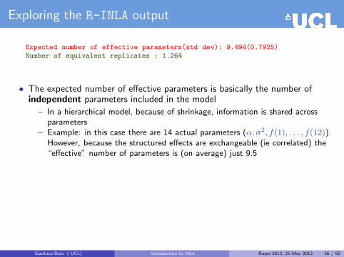
Exploring the R-INLA output
Expected number of effective parameters(std dev): 9.494(0.7925)Number of equivalent replicates : 1.264
• The expected number of effective parameters is basically the number ofindependent parameters included in the model
– In a hierarchical model, because of shrinkage, information is shared acrossparameters
– Example: in this case there are 14 actual parameters (α, σ2, f(1), . . . , f(12)).However, because the structured effects are exchangeable (ie correlated) the“effective” number of parameters is (on average) just 9.5
Gianluca Baio ( UCL) Introduction to INLA Bayes 2013, 21 May 2013 56 / 92
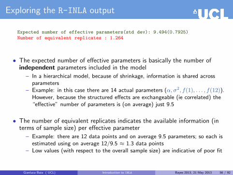
Exploring the R-INLA output
Expected number of effective parameters(std dev): 9.494(0.7925)Number of equivalent replicates : 1.264
• The expected number of effective parameters is basically the number ofindependent parameters included in the model
– In a hierarchical model, because of shrinkage, information is shared acrossparameters
– Example: in this case there are 14 actual parameters (α, σ2, f(1), . . . , f(12)).However, because the structured effects are exchangeable (ie correlated) the“effective” number of parameters is (on average) just 9.5
• The number of equivalent replicates indicates the available information (interms of sample size) per effective parameter
– Example: there are 12 data points and on average 9.5 parameters; so each isestimated using on average 12/9.5 ≈ 1.3 data points
– Low values (with respect to the overall sample size) are indicative of poor fit
Gianluca Baio ( UCL) Introduction to INLA Bayes 2013, 21 May 2013 56 / 92

Exploring the R-INLA output
Marginal Likelihood: -54.28CPO and PIT are computed
• R-INLA can produce two types of “leave-one-out” measures of fit1 Conditional Predictive Ordinate (CPO): p(yi | y−i)
• “Extreme” values for CPO indicate a surprising observation
2 Probability Integral Transforms (PIT): Pr(ynewi ≤ yi | y−i)• “Extreme” values for PIT indicate outliers• A histogram of PIT that does not look Uniformly distributed indicate lack of fit
for the current model
Gianluca Baio ( UCL) Introduction to INLA Bayes 2013, 21 May 2013 57 / 92

Exploring the R-INLA output
Marginal Likelihood: -54.28CPO and PIT are computed
• R-INLA can produce two types of “leave-one-out” measures of fit1 Conditional Predictive Ordinate (CPO): p(yi | y−i)
• “Extreme” values for CPO indicate a surprising observation
2 Probability Integral Transforms (PIT): Pr(ynewi ≤ yi | y−i)• “Extreme” values for PIT indicate outliers• A histogram of PIT that does not look Uniformly distributed indicate lack of fit
for the current model
• If the optioncontrol.compute=list(cpo=TRUE)
is added to the call to the function inla then the resulting object containsvalues for CPO and PIT, which can then be post-processed
– NB: for the sake of model checking, it is useful to to increase the accuracy ofthe estimation for the tails of the marginal distributions
– This can be done by adding the option
control.inla = list(strategy = "laplace", npoints = 21)
to add more evaluation points (npoints=21) instead of the defaultnpoints=9
Gianluca Baio ( UCL) Introduction to INLA Bayes 2013, 21 May 2013 57 / 92

Exploring the R-INLA output
0 20 40 60 80 100
0.0
0.4
0.8
The PIT−values, n.fail0
index
Pro
babi
lity
The PIT−values, n.fail0
Probability
Fre
quen
cy
0.0 0.2 0.4 0.6 0.8 1.0
02
46
8
0 20 40 60 80 100
02
46
812
The CPO−values, n.fail0
index
Pro
babi
lity
Histogram of the CPO−values, n.fail0
Probability
Fre
quen
cy
0 2 4 6 8 10 12
02
46
812
Gianluca Baio ( UCL) Introduction to INLA Bayes 2013, 21 May 2013 58 / 92
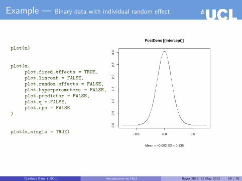
Example — Binary data with individual random effect
plot(m)
plot(m,plot.fixed.effects = TRUE,plot.lincomb = FALSE,plot.random.effects = FALSE,plot.hyperparameters = FALSE,plot.predictor = FALSE,plot.q = FALSE,plot.cpo = FALSE
)
plot(m,single = TRUE)−0.5 0.0 0.5
0.0
0.5
1.0
1.5
2.0
2.5
3.0
PostDens [(Intercept)]
Mean = −0.002 SD = 0.136
Gianluca Baio ( UCL) Introduction to INLA Bayes 2013, 21 May 2013 59 / 92
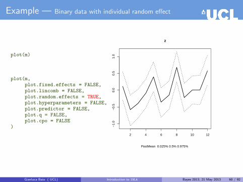
Example — Binary data with individual random effect
plot(m)
plot(m,plot.fixed.effects = FALSE,plot.lincomb = FALSE,plot.random.effects = TRUE,plot.hyperparameters = FALSE,plot.predictor = FALSE,plot.q = FALSE,plot.cpo = FALSE
)
2 4 6 8 10 12
−1.
0−
0.5
0.0
0.5
1.0
z
PostMean 0.025% 0.5% 0.975%
Gianluca Baio ( UCL) Introduction to INLA Bayes 2013, 21 May 2013 60 / 92

Manipulating the results from R-INLA
• The elements of the object m can be used for post-processing
m$summary.fixed
mean sd 0.025quant 0.5quant 0.975quant kld(Intercept) -0.002092578 0.1360447 -0.2720331 -0.002101465 0.2680023 1.866805e-08
m$summary.random
$zID mean sd 0.025quant 0.5quant 0.975quant kld
1 1 0.117716597 0.2130482 -0.29854459 0.116540837 0.54071007 1.561929e-062 2 -0.582142549 0.2328381 -1.05855344 -0.575397613 -0.14298960 3.040586e-053 3 -0.390419424 0.2159667 -0.82665552 -0.386498698 0.02359256 1.517773e-05
4 4 -0.087199172 0.2174477 -0.51798771 -0.086259111 0.33838724 7.076793e-075 5 0.392724605 0.2220260 -0.03217954 0.388462164 0.84160800 1.604348e-05
6 6 -0.353323459 0.2210244 -0.79933142 -0.349483252 0.07088015 1.242953e-057 7 -0.145238917 0.2122322 -0.56726042 -0.143798605 0.26859415 2.047815e-068 8 0.679294456 0.2279863 0.25076022 0.672226639 1.14699903 4.145645e-05
9 9 -0.214441626 0.2141299 -0.64230245 -0.212274011 0.20094086 4.577080e-0610 10 0.001634115 0.2131451 -0.41797579 0.001622300 0.42152562 4.356243e-09
11 11 0.001593724 0.2190372 -0.42961274 0.001581019 0.43309253 3.843622e-0912 12 0.580008923 0.2267330 0.15173745 0.573769187 1.04330359 3.191737e-05
Gianluca Baio ( UCL) Introduction to INLA Bayes 2013, 21 May 2013 61 / 92

Manipulating the results from R-INLA
alpha <- m$marginals.fixed[[1]]plot(inla.smarginal(alpha),t="l")
Marginal posterior: p(α | y)
−0.5 0.0 0.50.
00.
51.
01.
52.
02.
53.
0
Gianluca Baio ( UCL) Introduction to INLA Bayes 2013, 21 May 2013 62 / 92

Manipulating the results from R-INLA
alpha <- m$marginals.fixed[[1]]plot(inla.smarginal(alpha),t="l")
inla.qmarginal(0.05,alpha)[1] -0.2257259
Marginal posterior: p(α | y)
−0.5 0.0 0.50.
00.
51.
01.
52.
02.
53.
0
Gianluca Baio ( UCL) Introduction to INLA Bayes 2013, 21 May 2013 62 / 92

Manipulating the results from R-INLA
alpha <- m$marginals.fixed[[1]]plot(inla.smarginal(alpha),t="l")
inla.qmarginal(0.05,alpha)[1] -0.2257259
inla.pmarginal(-.2257259,alpha)[1] 0.04999996
inla.dmarginal(0,alpha)[1] 3.055793
inla.rmarginal(4,alpha)[1] 0.05307452 0.07866796 -0.09931744 -0.02027463
Gianluca Baio ( UCL) Introduction to INLA Bayes 2013, 21 May 2013 62 / 92

Example — Binary data with individual random effect
NB: INLA works by default with precisions
plot(m,plot.fixed.effects = FALSE,plot.lincomb = FALSE,plot.random.effects = FALSE,plot.hyperparameters = TRUE,plot.predictor = FALSE,plot.q = FALSE,plot.cpo = FALSE
)
0 20 40 60 80
0.00
0.02
0.04
0.06
0.08
0.10
0.12
0.14
PostDens [Precision for z]
Gianluca Baio ( UCL) Introduction to INLA Bayes 2013, 21 May 2013 63 / 92

Example — Binary data with individual random effect
NB: INLA works by default with precisions
plot(m,plot.fixed.effects = FALSE,plot.lincomb = FALSE,plot.random.effects = FALSE,plot.hyperparameters = TRUE,plot.predictor = FALSE,plot.q = FALSE,plot.cpo = FALSE
)
0 20 40 60 80
0.00
0.02
0.04
0.06
0.08
0.10
0.12
0.14
PostDens [Precision for z]
Problem: usually, we want to make inference on more interpretable parameters,eg standard deviations
Gianluca Baio ( UCL) Introduction to INLA Bayes 2013, 21 May 2013 63 / 92

Example — Binary data with individual random effect
• Using some built-in INLA functions
– model$marginals.hyperpar
– inla.expectation
– inla.rmarginal
it is possible to compute the structured variability, for example on thestandard deviation scale, based on nsamples (default=1000) MC simulationsfrom the estimated precision
s <- inla.contrib.sd(m,nsamples=1000)s$hyper
mean sd 2.5% 97.5%sd for z 0.416862 0.1098968 0.2332496 0.6478648
Gianluca Baio ( UCL) Introduction to INLA Bayes 2013, 21 May 2013 64 / 92

Example — Binary data with individual random effect
• Using some built-in INLA functions
– model$marginals.hyperpar
– inla.expectation
– inla.rmarginal
it is possible to compute the structured variability, for example on thestandard deviation scale, based on nsamples (default=1000) MC simulationsfrom the estimated precision
s <- inla.contrib.sd(m,nsamples=1000)s$hyper
mean sd 2.5% 97.5%sd for z 0.416862 0.1098968 0.2332496 0.6478648
• The object s contains a vector of simulations from the induced posteriordistribution for the standard deviation scale, than can then be used for plots
hist(s$samples)plot(density(s$samples,bw=.1),xlab="sigma",main="")
Gianluca Baio ( UCL) Introduction to INLA Bayes 2013, 21 May 2013 64 / 92
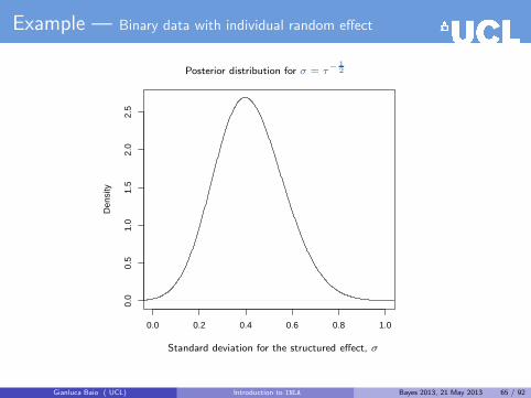
Example — Binary data with individual random effect
Posterior distribution for σ = τ− 1
2
0.0 0.2 0.4 0.6 0.8 1.0
0.0
0.5
1.0
1.5
2.0
2.5
Den
sity
Standard deviation for the structured effect, σ
Gianluca Baio ( UCL) Introduction to INLA Bayes 2013, 21 May 2013 65 / 92

Example — Binary data with individual random effect
If we wanted to perform MCMC on this model, we could
1 Program it in JAGS/BUGS and save it as model.txt
model {for (i in 1:n) {
y[i] ∼ dbinom(pi[i],Ntrials[i])logit(pi[i]) <- alpha+f[i]f[i] ∼ dnorm(0,tau)
}alpha ∼ dnorm(0,.001)
log.sigma ∼ dunif(0,10000)sigma <- exp(log.sigma)
tau <- pow(sigma,-2)}
Gianluca Baio ( UCL) Introduction to INLA Bayes 2013, 21 May 2013 66 / 92

Example — Binary data with individual random effect
If we wanted to perform MCMC on this model, we could
1 Program it in JAGS/BUGS and save it as model.txt
model {for (i in 1:n) {
y[i] ∼ dbinom(pi[i],Ntrials[i])logit(pi[i]) <- alpha+f[i]f[i] ∼ dnorm(0,tau)
}alpha ∼ dnorm(0,.001)
log.sigma ∼ dunif(0,10000)sigma <- exp(log.sigma)
tau <- pow(sigma,-2)}
2 In R, use the library R2jags (or R2WinBUGS) to interface with the MCMC software
library(R2jags)filein <- "model.txt"
dataJags <- list(y=y,n=n,Ntrials=Ntrials,prec=prec)params <- c("sigma","tau","f","pi","alpha")
inits <- function(){ list(log.sigma=runif(1),alpha=rnorm(1),f=rnorm(n,0,1)) }n.iter <- 100000
n.burnin <- 9500n.thin <- floor((n.iter-n.burnin)/500)mj <- jags(dataJags, inits, params, model.file=filein,n.chains=2, n.iter, n.burnin,
n.thin, DIC=TRUE, working.directory=working.dir, progress.bar="text")print(mj,digits=3,intervals=c(0.025, 0.975))
Gianluca Baio ( UCL) Introduction to INLA Bayes 2013, 21 May 2013 66 / 92

Example — Binary data with individual random effect
Inference for Bugs model at "model.txt", fit using jags,
2 chains, each with 1e+05 iterations (first 9500 discarded), n.thin = 181n.sims = 1000 iterations saved (Time to run: 4.918 sec)
mu.vect sd.vect 2.5% 97.5% Rhat n.effalpha -0.005 0.146 -0.270 0.292 1.001 1000
f[1] 0.122 0.220 -0.347 0.582 1.001 1000f[2] -0.564 0.238 -1.051 -0.115 1.008 190
f[3] -0.386 0.229 -0.880 0.050 1.000 1000f[4] -0.086 0.225 -0.549 0.367 1.002 780
f[5] 0.392 0.227 -0.047 0.828 1.002 870f[6] -0.351 0.229 -0.805 0.081 1.000 1000f[7] -0.141 0.221 -0.578 0.286 1.001 1000
f[8] 0.672 0.236 0.246 1.200 1.002 860f[9] -0.224 0.210 -0.643 0.178 1.000 1000
f[10] 0.016 0.219 -0.396 0.463 1.006 1000f[11] -0.001 0.221 -0.441 0.416 1.002 780f[12] 0.585 0.245 0.153 1.093 1.001 1000
sigma 0.414 0.120 0.230 0.693 1.000 1000tau 7.415 4.546 2.080 18.951 1.000 1000
deviance 72.378 5.497 64.016 84.715 1.000 1000
For each parameter, n.eff is a crude measure of effective sample size,and Rhat is the potential scale reduction factor (at convergence, Rhat=1).
DIC info (using the rule, pD = var(deviance)/2)pD = 15.1 and DIC = 87.5
DIC is an estimate of expected predictive error (lower deviance is better).
Gianluca Baio ( UCL) Introduction to INLA Bayes 2013, 21 May 2013 67 / 92

Example — Binary data with individual random effect
Structured effects−1.0 −0.5 0.0 0.5 1.0
f(1)
f(2)
f(3)
f(4)
f(5)
f(6)
f(7)
f(8)
f(9)
f(10)
f(11)
f(12) JAGSINLA
Gianluca Baio ( UCL) Introduction to INLA Bayes 2013, 21 May 2013 68 / 92

Example — Binary data with individual random effect
Posterior distribution for σ = τ− 1
2
0.0 0.2 0.4 0.6 0.8 1.0
0.0
0.5
1.0
1.5
2.0
2.5
3.0
3.5
Den
sity
JAGSINLA
Standard deviation for the structured effect, σ
Gianluca Baio ( UCL) Introduction to INLA Bayes 2013, 21 May 2013 69 / 92

Example — Binary data with individual random effect
• R-INLA allows to make predictive inference based on the observed model
• Suppose for example that the (n+ 1)−th value is not (yet) observed for theresponse variable y
– NB: for R-INLA, a missing value in the response means no likelihoodcontribution
Gianluca Baio ( UCL) Introduction to INLA Bayes 2013, 21 May 2013 70 / 92

Example — Binary data with individual random effect
• R-INLA allows to make predictive inference based on the observed model
• Suppose for example that the (n+ 1)−th value is not (yet) observed for theresponse variable y
– NB: for R-INLA, a missing value in the response means no likelihoodcontribution
• We can code this in R, by augmenting the original datasety[n+1] <- NANtrials[n+1] <- sample(c(80:100),size=1,replace=TRUE)data2 <- data.frame(y=y,z=1:(n+1),Ntrials=Ntrials)
formula2 = y ∼ f(z,model="iid",hyper=list(list(prior="flat")))m2=inla(formula2,data=data2,
family="binomial",Ntrials=Ntrials,control.predictor = list(compute = TRUE))
summary(m2)
Gianluca Baio ( UCL) Introduction to INLA Bayes 2013, 21 May 2013 70 / 92

Example — Binary data with individual random effect
Time used:Pre-processing Running inla Post-processing Total
0.0883 0.0285 0.0236 0.1404(0.2258) (0.0263) (0.0744) (0.3264)
Fixed effects:mean sd 0.025quant 0.5quant 0.975quant kld
(Intercept) -0.0021 0.136 -0.272 -0.0021 0.268 0(-0.0021) (0.136) (-0.272) (-0.0021) (0.268) (0)
Random effects:Name Model
z IID model
Model hyperparameters:mean sd 0.025quant 0.5quant 0.975quant
Precision for z 7.130 4.087 2.168 6.186 17.599
(7.130) (4.087) (2.168) (6.168) (17.599)
Expected number of effective parameters(std dev): 9.494(0.7925)Number of equivalent replicates : 1.264
Marginal Likelihood: -54.28CPO and PIT are computed
Posterior marginals for linear predictor and fitted values computed
Gianluca Baio ( UCL) Introduction to INLA Bayes 2013, 21 May 2013 71 / 92

Example — Binary data with individual random effect
• The estimated value for the predictive distribution can be retrieved using thefollowing code
pred <- m2$marginals.linear.predictor[[n+1]]plot(pred,xlab="",ylab="Density")lines(inla.smarginal(pred))
which can be used to generate, eg a graph of the predictive density
−2 −1 0 1 2
0.0
0.2
0.4
0.6
0.8
Den
sity
Gianluca Baio ( UCL) Introduction to INLA Bayes 2013, 21 May 2013 72 / 92

Specifying the model — options
• It is possible to specify link functions that are different from the default usedby R-INLA
• This is done by specifying suitable values for the option control.family tothe call to inla, eg
m = inla(formula, data=data, family="binomial", Ntrials=Ntrials,control.predictor=list(compute=TRUE),control.family = list(link = "probit"))
Gianluca Baio ( UCL) Introduction to INLA Bayes 2013, 21 May 2013 73 / 92

Specifying the model — options
• It is possible to specify link functions that are different from the default usedby R-INLA
• This is done by specifying suitable values for the option control.family tothe call to inla, eg
m = inla(formula, data=data, family="binomial", Ntrials=Ntrials,control.predictor=list(compute=TRUE),control.family = list(link = "probit"))
• More details are available on the R-INLA website:
– http://www.r-inla.org/models/likelihoods
Gianluca Baio ( UCL) Introduction to INLA Bayes 2013, 21 May 2013 73 / 92

Specifying the model — options
• R-INLA has a set of default priors for the different components of theLGM/GMRF
• For example, in a standard hierarchical formulation, R-INLA assumes
– Unstructured (“fixed”) effects: β ∼ Normal(0, 0.001)– Structured (“random”) effects: f(zi) ∼ Normal(0, τ )
Structured (“random”) effects: log τ ∼ logGamma(1, 0.00005)
• NB: It is possible to see the default settings using the function
inla.model.properties(<name>, <section>)
Gianluca Baio ( UCL) Introduction to INLA Bayes 2013, 21 May 2013 74 / 92

Specifying the model — options
• R-INLA has a set of default priors for the different components of theLGM/GMRF
• For example, in a standard hierarchical formulation, R-INLA assumes
– Unstructured (“fixed”) effects: β ∼ Normal(0, 0.001)– Structured (“random”) effects: f(zi) ∼ Normal(0, τ )
Structured (“random”) effects: log τ ∼ logGamma(1, 0.00005)
• NB: It is possible to see the default settings using the function
inla.model.properties(<name>, <section>)
• However, there is a wealth of possible formulations that the user can specify,especially for the hyperpriors
• More details are available on the R-INLA website:
– http://www.r-inla.org/models/likelihoods
– http://www.r-inla.org/models/latent-models
– http://www.r-inla.org/models/priors
Gianluca Baio ( UCL) Introduction to INLA Bayes 2013, 21 May 2013 74 / 92

Specifying the model — options
Models for the observed data
Model NameNegative Binomial nbinomialPoisson poissonBinomial binomialClustered Binomial cbinomialGaussian gaussianSkew Normal snLaplace laplaceStudent-t TGaussian model for stochastic volatility stochvolStudent-t model for stochastic volatility stochvol.tNIG model for stochastic volatility stochvol.nigZero inflated Poisson zeroinflated.poisson.x (x=0,1,2)Zero inflated Binomial zeroinflated.binomial.x (x=0,1)Zero inflated negative Binomial zeroinflated.nbinomial.x (x=0,1,2)Zero inflated beta binomial (type 2) zeroinflated.betabinomial.2Generalised extreme value distribution (GEV) gevBeta betaGamma gammaBeta-Binomial betabinomialLogistic distribution logisticExponential (Survival models) exponentialWeibull (Survival model) weibullLogLogistic (Survival model) loglogisticLogNormal (Survival model) lognormalCox model (Survival model) coxph
Gianluca Baio ( UCL) Introduction to INLA Bayes 2013, 21 May 2013 75 / 92
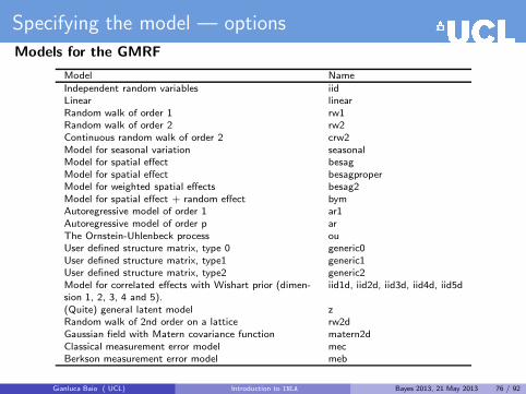
Specifying the model — options
Models for the GMRF
Model Name
Independent random variables iidLinear linearRandom walk of order 1 rw1Random walk of order 2 rw2Continuous random walk of order 2 crw2Model for seasonal variation seasonalModel for spatial effect besagModel for spatial effect besagproperModel for weighted spatial effects besag2Model for spatial effect + random effect bymAutoregressive model of order 1 ar1Autoregressive model of order p arThe Ornstein-Uhlenbeck process ouUser defined structure matrix, type 0 generic0User defined structure matrix, type1 generic1User defined structure matrix, type2 generic2Model for correlated effects with Wishart prior (dimen-sion 1, 2, 3, 4 and 5).
iid1d, iid2d, iid3d, iid4d, iid5d
(Quite) general latent model zRandom walk of 2nd order on a lattice rw2dGaussian field with Matern covariance function matern2dClassical measurement error model mecBerkson measurement error model meb
Gianluca Baio ( UCL) Introduction to INLA Bayes 2013, 21 May 2013 76 / 92

Specifying the model — options
Models for the hyper-parameters
Model NameNormal distribution normal, gaussianLog-gamma distribution loggammaImproper flat prior flatTruncated Normal distribution logtnormal, logtgaussianImproper flat prior on the log scale logflatImproper flat prior on the 1/ log scale logiflatWishart prior wishartBeta for correlations betacorrelationLogit of a Beta logitbetaDefine your own prior expression:
Gianluca Baio ( UCL) Introduction to INLA Bayes 2013, 21 May 2013 77 / 92

Internal vs user scale
• Hyper-parameters (eg correlation coefficients ρ or precisions τ) arerepresented internally using a suitable transformation, eg
ψ1 = log(τ)
orψ2 = log
(1 + ρ
1− ρ
)
to improve symmetry and approximate Normality
Gianluca Baio ( UCL) Introduction to INLA Bayes 2013, 21 May 2013 78 / 92

Internal vs user scale
• Hyper-parameters (eg correlation coefficients ρ or precisions τ) arerepresented internally using a suitable transformation, eg
ψ1 = log(τ)
orψ2 = log
(1 + ρ
1− ρ
)
to improve symmetry and approximate Normality
• Initial values are given on the internal scale
• Priors are also defined on the internal scale
• So, when specifying custom values, care is needed!
Gianluca Baio ( UCL) Introduction to INLA Bayes 2013, 21 May 2013 78 / 92

Specifying the prior (1)
Consider the model
yi | θi, σ2 ∼ Normal(θi, σ
2)
θi = α+ βxi
α, βiid∼ Normal(0, 0.001)
log τ = − logσ2 ∼ logGamma(1, 0.01)
n=100a = 1; b = 1x = rnorm(n)eta = a + b*xtau = 100scale = exp(rnorm(n))prec = scale*tauy = rnorm(n, mean = eta, sd = 1/sqrt(prec))data = list(y=y, x=x)formula = y ∼ 1 + xresult = inla(formula, family = "gaussian", data = data,
control.family = list(hyper = list(prec = list(prior = "loggamma",param = c(1,0.01),initial = 2))),
scale=scale, keep=TRUE)summary(result)
Gianluca Baio ( UCL) Introduction to INLA Bayes 2013, 21 May 2013 79 / 92

Specifying the prior (1)
Time used:Pre-processing Running inla Post-processing Total
0.0776 0.0828 0.0189 0.1793
Fixed effects:mean sd 0.025quant 0.5quant 0.975quant kld
(Intercept) 1.0013 0.0074 0.9868 1.0013 1.0158 0x 0.9936 0.0075 0.9788 0.9936 1.0083 0
The model has no random effects
Model hyperparameters:mean sd 0.025quant 0.5quant 0.975quant
Precision for the Gaussian observations 108.00 15.34 80.60 107.09 140.74
Expected number of effective parameters(std dev): 2.298(0.0335)Number of equivalent replicates : 43.52
Marginal Likelihood: 83.86CPO and PIT are computed
Gianluca Baio ( UCL) Introduction to INLA Bayes 2013, 21 May 2013 80 / 92

Specifying the prior (2)
Consider the model
yi | µ, σ2 ∼ Normal(µ, σ2)
µ ∼ Normal(0, 0.001)
log τ = − logσ2 ∼ Normal(0, 1)
n = 10y = rnorm(n)formula = y ∼ 1result = inla(formula, data = data.frame(y),
control.family = list(hyper = list(prec = list(prior = "normal",param = c(0,1))))
)summary(result)
Gianluca Baio ( UCL) Introduction to INLA Bayes 2013, 21 May 2013 81 / 92

Specifying the prior (2)
Consider the model
yi | µ, σ2 ∼ Normal(µ, σ2)
µ ∼ Normal(0, 0.001)
log τ = − logσ2 ∼ Normal(0, 1)
n = 10y = rnorm(n)formula = y ∼ 1result = inla(formula, data = data.frame(y),
control.family = list(hyper = list(prec = list(prior = "normal",param = c(0,1))))
)summary(result)
• NB: INLA thinks in terms of LGMs and GMRFs
• Thus, the common mean for all the observations is specified in terms of aregression!
Gianluca Baio ( UCL) Introduction to INLA Bayes 2013, 21 May 2013 81 / 92

Specifying the prior (2)
Time used:Pre-processing Running inla Post-processing Total
0.0740 0.0214 0.0221 0.1175
Fixed effects:mean sd 0.025quant 0.5quant 0.975quant kld
(Intercept) -0.3853 0.4077 -1.1939 -0.3853 0.4237 0
The model has no random effects
Model hyperparameters:mean sd 0.025quant 0.5quant 0.975quant
Precision for the Gaussian observations 0.6512 0.268 0.2590 0.6089 1.2919
Expected number of effective parameters(std dev): 1.00(0.00)Number of equivalent replicates : 9.999
Marginal Likelihood: -17.30CPO and PIT are computed
Gianluca Baio ( UCL) Introduction to INLA Bayes 2013, 21 May 2013 82 / 92

Specifying the prior (2)
Running the model in JAGS
model {for (i in 1:n) {
y[i] ∼ dnorm(mu,tau)
}mu ∼ dnorm(0,0.001)
log.tau ∼ dnorm(0,1)tau <- exp(log.tau)
}
produces similar results
Inference for Bugs model at "modelHyperPriorNormal.txt", fit using jags,2 chains, each with 1e+05 iterations (first 9500 discarded), n.thin = 181n.sims = 1000 iterations saved
mu.vect sd.vect 2.5% 97.5% Rhat n.effmu -0.384 0.447 -1.293 0.555 1.000 1000
tau 0.642 0.258 0.233 1.240 1.006 1000deviance 34.507 1.930 32.645 39.897 1.002 650
For each parameter, n.eff is a crude measure of effective sample size,and Rhat is the potential scale reduction factor (at convergence, Rhat=1).
DIC info (using the rule, pD = var(deviance)/2)
pD = 1.9 and DIC = 36.4DIC is an estimate of expected predictive error (lower deviance is better).
Gianluca Baio ( UCL) Introduction to INLA Bayes 2013, 21 May 2013 83 / 92

Specifying the prior (2)
• We can also assume different priors for the unstructured (“fixed”) effects, egsuppose we want to fit the model
yi | µ, σ2 ∼ Normal(µ, σ2)
µ ∼ Normal(10, 4)
log τ = − log σ2 ∼ Normal(0, 1)
Gianluca Baio ( UCL) Introduction to INLA Bayes 2013, 21 May 2013 84 / 92

Specifying the prior (2)
• We can also assume different priors for the unstructured (“fixed”) effects, egsuppose we want to fit the model
yi | µ, σ2 ∼ Normal(µ, σ2)
µ ∼ Normal(10, 4)
log τ = − log σ2 ∼ Normal(0, 1)
• This can be done by using the option control.fixed, eg
result = inla(formula, data = data.frame(y),control.family = list(hyper = list(
prec = list(prior = "normal",param = c(0, 1))))control.fixed=list(
mean.intercept=10,prec.intercept=4))
• NB: If the model contains fixed effects for some covariates, non-default priorscan be included using the option
control.fixed=list(mean=list(value),prec=list(value))
Gianluca Baio ( UCL) Introduction to INLA Bayes 2013, 21 May 2013 84 / 92

Specifying the prior (2)
Time used:Pre-processing Running inla Post-processing Total
0.0747 0.0311 0.0164 0.1222
Fixed effects:mean sd 0.025quant 0.5quant 0.975quant kld
(Intercept) 9.5074 0.502 8.5249 9.5067 10.4935 0-0.3853 0.407 -1.1939 -0.3853 0.4237 0
The model has no random effects
Model hyperparameters:mean sd 0.025quant 0.5quant 0.975quant
Precision for the Gaussian observations 0.0218 0.007 0.0105 0.0208 0.03910.6512 0.268 0.2590 0.6089 1.2919
Expected number of effective parameters(std dev): 0.0521(0.0129)1.0000(0.0000)
Number of equivalent replicates : 192.059.9999
Marginal Likelihood: 153.84-17.30
CPO and PIT are computed
Gianluca Baio ( UCL) Introduction to INLA Bayes 2013, 21 May 2013 85 / 92

Improving the estimation of the hyperparameters
• As mentioned earlier, for computational reasons, by default INLA uses arelatively rough grid to estimate the marginal posterior for thehyperparameters p(ψ | y)
• This is generally good enough, but the procedure can be refined
Gianluca Baio ( UCL) Introduction to INLA Bayes 2013, 21 May 2013 86 / 92

Improving the estimation of the hyperparameters
• As mentioned earlier, for computational reasons, by default INLA uses arelatively rough grid to estimate the marginal posterior for thehyperparameters p(ψ | y)
• This is generally good enough, but the procedure can be refined
• After the model has been estimated using the standard procedure, it ispossible to increase precision in the estimation by re-fitting it using thecommand
inla.hyperpar(m, options)
• This modifies the estimation for the hyperparameters and (potentially, butnot necessarily!) that for the parameters
Gianluca Baio ( UCL) Introduction to INLA Bayes 2013, 21 May 2013 86 / 92

A more complex model
• Consider the classic model for seizure counts in a RCT of anti-conversanttherapy in epilepsy (“Epil” in the BUGS manual)
• The data are as follows
Patient Visit 1 Visit 2 Visit 3 Visit 4 Trt Base Age1 5 3 3 3 0 11 312 3 5 3 3 0 11 30. . . . . . . . . . . . . . . . . . . . . . . .59 1 4 3 2 1 12 37
• We replicate the model presented in the BUGS manual, which uses slightlymodified version of the covariates
Gianluca Baio ( UCL) Introduction to INLA Bayes 2013, 21 May 2013 87 / 92

A more complex model
We model
yjk ∼ Poisson(µjk)
log(µjk) = α0 + α1 log(Bj/4) + α2Trtj +
α3Trtj × log(Bj/4) + α4 log(Agej) +
α5V 4k + uj + vik
α0, . . . α5iid∼ Normal(0, τα), τα known
uj ∼ Normal(0, τu), τu ∼ Gamma(au, bu)
vjk ∼ Normal(0, τv), τv ∼ Gamma(av, bv)
Gianluca Baio ( UCL) Introduction to INLA Bayes 2013, 21 May 2013 88 / 92

A more complex model
We model
yjk ∼ Poisson(µjk)
log(µjk) = α0 + α1 log(Bj/4) + α2Trtj +
α3Trtj × log(Bj/4) + α4 log(Agej) +
α5V 4k + uj + vik
α0, . . . α5iid∼ Normal(0, τα), τα known
uj ∼ Normal(0, τu), τu ∼ Gamma(au, bu)
vjk ∼ Normal(0, τv), τv ∼ Gamma(av, bv)
α = (α0, . . . α5) indicates a set of “fixed” effects for the relevant (re-scaled)covariates
Gianluca Baio ( UCL) Introduction to INLA Bayes 2013, 21 May 2013 88 / 92
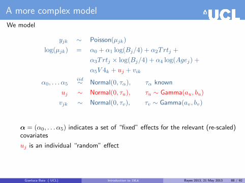
A more complex model
We model
yjk ∼ Poisson(µjk)
log(µjk) = α0 + α1 log(Bj/4) + α2Trtj +
α3Trtj × log(Bj/4) + α4 log(Agej) +
α5V 4k + uj + vik
α0, . . . α5iid∼ Normal(0, τα), τα known
uj ∼ Normal(0, τu), τu ∼ Gamma(au, bu)
vjk ∼ Normal(0, τv), τv ∼ Gamma(av, bv)
α = (α0, . . . α5) indicates a set of “fixed” effects for the relevant (re-scaled)covariates
uj is an individual “random” effect
Gianluca Baio ( UCL) Introduction to INLA Bayes 2013, 21 May 2013 88 / 92
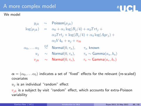
A more complex model
We model
yjk ∼ Poisson(µjk)
log(µjk) = α0 + α1 log(Bj/4) + α2Trtj +
α3Trtj × log(Bj/4) + α4 log(Agej) +
α5V 4k + uj + vik
α0, . . . α5iid∼ Normal(0, τα), τα known
uj ∼ Normal(0, τu), τu ∼ Gamma(au, bu)
vjk ∼ Normal(0, τv), τv ∼ Gamma(av, bv)
α = (α0, . . . α5) indicates a set of “fixed” effects for the relevant (re-scaled)covariates
uj is an individual “random” effect
vjk is a subject by visit “random” effect, which accounts for extra-Poissonvariability
Gianluca Baio ( UCL) Introduction to INLA Bayes 2013, 21 May 2013 88 / 92

A more complex model
data(Epil)head(Epil,n=3)
y Trt Base Age V4 rand Ind1 5 0 11 31 0 1 12 3 0 11 31 0 2 13 3 0 11 31 0 3 1
formula <- y ∼ log(Base/4) + Trt +I(Trt * log(Base/4)) + log(Age) + V4 +f(Ind, model = "iid") + f(rand, model="iid")
m <- inla(formula, family="poisson", data = Epil)
• NB: The variable Ind indicates the individual random effect uj , while thevariable rand is used to model the subject by visit random effect vjk
• Interactions can be indicated in the R formula using the notation
I(var1 * var2)
• The model assumes that the two structured effects are independent. This canbe relaxed and a joint model can be used instead
Gianluca Baio ( UCL) Introduction to INLA Bayes 2013, 21 May 2013 89 / 92
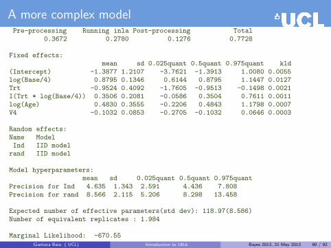
A more complex modelPre-processing Running inla Post-processing Total
0.3672 0.2780 0.1276 0.7728
Fixed effects:mean sd 0.025quant 0.5quant 0.975quant kld
(Intercept) -1.3877 1.2107 -3.7621 -1.3913 1.0080 0.0055log(Base/4) 0.8795 0.1346 0.6144 0.8795 1.1447 0.0127Trt -0.9524 0.4092 -1.7605 -0.9513 -0.1498 0.0021I(Trt * log(Base/4)) 0.3506 0.2081 -0.0586 0.3504 0.7611 0.0011log(Age) 0.4830 0.3555 -0.2206 0.4843 1.1798 0.0007V4 -0.1032 0.0853 -0.2705 -0.1032 0.0646 0.0003
Random effects:Name ModelInd IID modelrand IID model
Model hyperparameters:mean sd 0.025quant 0.5quant 0.975quant
Precision for Ind 4.635 1.343 2.591 4.436 7.808Precision for rand 8.566 2.115 5.206 8.298 13.458
Expected number of effective parameters(std dev): 118.97(8.586)Number of equivalent replicates : 1.984
Marginal Likelihood: -670.55
Gianluca Baio ( UCL) Introduction to INLA Bayes 2013, 21 May 2013 90 / 92
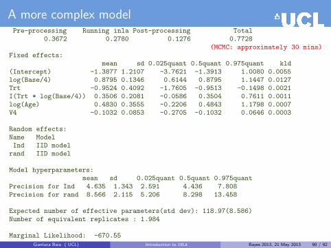
A more complex modelPre-processing Running inla Post-processing Total
0.3672 0.2780 0.1276 0.7728(MCMC: approximately 30 mins)
Fixed effects:mean sd 0.025quant 0.5quant 0.975quant kld
(Intercept) -1.3877 1.2107 -3.7621 -1.3913 1.0080 0.0055log(Base/4) 0.8795 0.1346 0.6144 0.8795 1.1447 0.0127Trt -0.9524 0.4092 -1.7605 -0.9513 -0.1498 0.0021I(Trt * log(Base/4)) 0.3506 0.2081 -0.0586 0.3504 0.7611 0.0011log(Age) 0.4830 0.3555 -0.2206 0.4843 1.1798 0.0007V4 -0.1032 0.0853 -0.2705 -0.1032 0.0646 0.0003
Random effects:Name ModelInd IID modelrand IID model
Model hyperparameters:mean sd 0.025quant 0.5quant 0.975quant
Precision for Ind 4.635 1.343 2.591 4.436 7.808Precision for rand 8.566 2.115 5.206 8.298 13.458
Expected number of effective parameters(std dev): 118.97(8.586)Number of equivalent replicates : 1.984
Marginal Likelihood: -670.55
Gianluca Baio ( UCL) Introduction to INLA Bayes 2013, 21 May 2013 90 / 92

Conclusions
• Integrated Nested Laplace Approximation is a very effective tool to estimateLGMs
– Estimation time can be much lower than for standard MCMC– Precision of estimation is usually higher than for standard MCMC
Gianluca Baio ( UCL) Introduction to INLA Bayes 2013, 21 May 2013 91 / 92

Conclusions
• Integrated Nested Laplace Approximation is a very effective tool to estimateLGMs
– Estimation time can be much lower than for standard MCMC– Precision of estimation is usually higher than for standard MCMC
• MCMC still provides a slightly more flexible approach
– Virtually any model can be fit using JAGS/BUGS– The range of priors available is wider in an MCMC setting than in INLA
– Documentation and examples is more extensive for standard MCMC models
• Nevertheless, INLA proves to be a very flexible tool, which is able to fit a verywide range of models
– Generalised linear (mixed) models– Log-Gaussian Cox processes– Survival analysis– Spline smoothing– Spatio-temporal models
• The INLA setup can be highly specialised (choice of data models, priors andhyperpriors) although this is a bit less intuitive than (most) MCMC models
Gianluca Baio ( UCL) Introduction to INLA Bayes 2013, 21 May 2013 91 / 92

Thank you!
Gianluca Baio ( UCL) Introduction to INLA Bayes 2013, 21 May 2013 92 / 92