ANIMATING CHARACTER NAVIGATION USING MOTION GRAPHS

A THESIS SUBMITTED TO

THE GRADUATE SCHOOL OF NATURAL AND APPLIED SCIENCES

OF

MIDDLE EAST TECHNICAL UNIVERSITY

BY

GAZIHAN ALANKUS

IN PARTIAL FULFILLMENT OF THE REQUIREMENTS

FOR

THE DEGREE OF MASTER OF SCIENCE

IN

COMPUTER ENGINEERING

JUNE 2005

Approval of the Graduate School of Natural and Applied Sciences

Prof. Dr. Canan OzgenDirector

I certify that this thesis satisfies all the requirements as a thesis for the degree ofMaster of Science.

Prof. Dr. Ayse KiperHead of Department

This is to certify that we have read this thesis and that in our opinion it is fullyadequate, in scope and quality, as a thesis for the degree of Master of Science

Assoc. Prof. Dr. Ferda NurAlpaslan

Supervisor

Examining Committee Members

Prof. Dr. Mehmet R. Tolun

Assoc. Prof. Dr. Veysi Isler

Assoc. Prof. Dr. Ferda Nur Alpaslan

Assist. Prof. Dr. Halit Oguztuzun

Dr. Aysenur Birturk

I hereby declare that all information in this document has been

obtained and presented in accordance with academic rules and ethical

conduct. I also declare that, as required by these rules and conduct,

I have fully cited and referenced all material and results that are not

original to this work.

Name, Last name :

Signature :

iii

ABSTRACT

ANIMATING CHARACTER NAVIGATION USING MOTION

GRAPHS

Alankus, Gazihan

M.Sc., Department of Computer Engineering

Supervisor: Assoc. Prof. Dr. Ferda Nur Alpaslan

June 2005, 60 Pages

Creating realistic human animations is a difficult and time consumig job. One

of the best solutions known is motion capture, which is an expensive process.

Manipulating existing motion data instead of capturing new data is an efficient

way of creating new human animations. In this thesis, we review the current

techniques for animation, navigation and ways of manipulating motion data. We

discuss strengths and weaknesses of interpolation techniques for creating new

motions. Then we present a system that uses existing motion data to create a

motion graph and automatically creates new motion data for character naviga-

tion suitable for user requirements. Finally, we give experimental results and

discuss possible uses of the system.

Keywords: Computer animation, computer graphics, motion planning

iv

OZ

HAREKET CIZGELERI KULLANILARAK KARAKTER YOL

BULMA ANIMASYONLARI URETILMESI

Alankus, Gazihan

Yuksek Lisans, Bilgisayar Muhendisligi Bolumu

Tez Yoneticisi: Doc. Dr. Ferda Nur Alpaslan

Haziran 2005, 60 Sayfa

Gercekci insan animasyonu yaratma zor ve vakit alıcı bir istir. Bilinen en iyi

cozumlerden biri, pahalı bir islem olan hareket yakalamadır. Yeni hareket yakala-

mak yerine var olan hareket verilerini degistirerek kullanmak, yeni hareketler

uretmek icin etkili bir yontemdir. Bu tezde, animasyon, yol bulma ve hareket

verilerini degistirme icin kullanılan teknikler gozden gecirilmistir. Yeni hareketler

uretmek icin kullanılan cesitli ic degerleme tekniklerinin iyi ve kotu yanları tartısıl-

mıstır. Daha sonra, var olan hareket verilerini kullanarak bir hareket cizgesi

olusturan ve kullanıcı kriterlerine uygun bir sekilde yol bulma icin otomatik olarak

hareket verisi ureten bir sistem sunulmustur. Son olarak deneysel sonuclar ver-

ilmis ve sistemin olası kullanım alanları tartısılmıstır.

Anahtar Kelimeler: Bilgisayar animasyonu, bilgisayar grafigi, hareket planlama

v

Table of Contents

PLAGIARISM . . . . . . . . . . . . . . . . . . . . . . . . . . . . . . . . iii

ABSTRACT . . . . . . . . . . . . . . . . . . . . . . . . . . . . . . . . . iv

OZ . . . . . . . . . . . . . . . . . . . . . . . . . . . . . . . . . . . . . . . . iv

TABLE OF CONTENTS . . . . . . . . . . . . . . . . . . . . . . . . . v

1 INTRODUCTION . . . . . . . . . . . . . . . . . . . . . . . . . . . . 1

2 COMPUTER ANIMATION . . . . . . . . . . . . . . . . . . . . . 3

2.1 Traditional Animation and Computer Animation . . . . . . . . . 4

2.2 2D Computer Animation . . . . . . . . . . . . . . . . . . . . . . . 5

2.3 3D Computer Animation . . . . . . . . . . . . . . . . . . . . . . . 5

2.3.1 Modeling . . . . . . . . . . . . . . . . . . . . . . . . . . . 6

2.3.2 Animation . . . . . . . . . . . . . . . . . . . . . . . . . . . 8

2.3.3 Rendering . . . . . . . . . . . . . . . . . . . . . . . . . . . 10

3 FULL BODY CHARACTER ANIMATION . . . . . . . . . . . . 11

3.1 Modeling . . . . . . . . . . . . . . . . . . . . . . . . . . . . . . . . 12

3.1.1 Hierarchical Modeling . . . . . . . . . . . . . . . . . . . . 12

3.2 Animation . . . . . . . . . . . . . . . . . . . . . . . . . . . . . . . 17

3.2.1 Keyframing . . . . . . . . . . . . . . . . . . . . . . . . . . 17

3.2.2 Physically Based Methods . . . . . . . . . . . . . . . . . . 25

3.2.3 Motion Capture . . . . . . . . . . . . . . . . . . . . . . . . 26

3.2.4 Motion Capture Based Methods . . . . . . . . . . . . . . . 27

3.3 Rendering . . . . . . . . . . . . . . . . . . . . . . . . . . . . . . . 32

vi

4 CHARACTER NAVIGATION . . . . . . . . . . . . . . . . . . . . 33

4.1 Motion Planning . . . . . . . . . . . . . . . . . . . . . . . . . . . 33

4.1.1 PRM . . . . . . . . . . . . . . . . . . . . . . . . . . . . . . 34

4.1.2 RRT . . . . . . . . . . . . . . . . . . . . . . . . . . . . . . 35

4.2 Character Navigation Using a Motion Graph . . . . . . . . . . . . 36

4.2.1 Related Work . . . . . . . . . . . . . . . . . . . . . . . . . 36

4.2.2 Our Approach . . . . . . . . . . . . . . . . . . . . . . . . . 37

5 PROPOSED SOLUTION . . . . . . . . . . . . . . . . . . . . . . . 39

5.1 Problem . . . . . . . . . . . . . . . . . . . . . . . . . . . . . . . . 39

5.2 Solution . . . . . . . . . . . . . . . . . . . . . . . . . . . . . . . . 39

5.3 Motion Graph . . . . . . . . . . . . . . . . . . . . . . . . . . . . . 40

5.3.1 The Distance Metric . . . . . . . . . . . . . . . . . . . . . 41

5.3.2 Finding Interpolation Regions . . . . . . . . . . . . . . . . 42

5.3.3 Interpolation . . . . . . . . . . . . . . . . . . . . . . . . . 43

5.3.4 Creation of the Motion Graph . . . . . . . . . . . . . . . . 49

5.4 Planning the Path . . . . . . . . . . . . . . . . . . . . . . . . . . 49

5.5 Planning the Motion . . . . . . . . . . . . . . . . . . . . . . . . . 51

5.6 Experimental Results . . . . . . . . . . . . . . . . . . . . . . . . . 53

6 CONCLUSION . . . . . . . . . . . . . . . . . . . . . . . . . . . . . . 57

REFERENCES . . . . . . . . . . . . . . . . . . . . . . . . . . . . . . . . 58

vii

CHAPTER 1

Introduction

3D Computer animation is a tool that has been a vital element of a number of

applications such as computer games, movies and virtual reality simulations. It

enables the user to view a life-like simulation of different events and improves

the quality of the experience. For example, a well prepared animated movie with

sounds provides a more impressive entertainment than a comic strip with still

images and captions. A well-animated character in a computer game makes it

more compelling and provides a realistic experience. A believeable virtual stunt

in a movie makes the movie more exciting anh lowers health risks of stuntmen.

Creating believeable motions for complex entities is a difficult task. There

are many things to consider when animating a complex entity. These include the

positions of the moving parts, their velocities in time and high level behaviors

created using primitive motions. Human characters are examples to complex

entities and are among the most frequently used elements in computer animations.

In addition to being complex, human motions have an important role in cog-

nitive science. In daily life, motions such as signs are a major way of communica-

tion after speech. In addition to using motion as a direct way of communication,

humans unconsciously extract meanings and feelings that are unconsciously in-

cluded in the motions of the subject. Therefore, if the animation of a character

gives the user the feeling of happiness and the character is supposed to be sad,

the coherence of the animation is affected in a negative way. Thus, animating

human characters requires special attention.

Creating human animations is a difficult task. If the animation to be created

contains complex patterns such as walking, the work to be done by animation

1

artists become even more demanding. Since motions like walking tend to be

repetitive, they can potentially be created in a more efficient way.

In this thesis, we review the current methods for creating human animations

and identify different parts of the animation pipeline. We then address the prob-

lem of navigating a walking human character in a realistic way. For this purpose

we repetitively use motion capture clips using a motion graph data structure.

We demonstrate our approach with experiments and discuss its strengths and

weaknesses.

2

CHAPTER 2

Computer Animation

The word ”animate” means ”give life to” [19]. ”Animating” can be used for mak-

ing puppets move with strings or making cartoon characters wander by certain

techniques. The word ”animation” is mostly used for the latter. In order to

convert a picture to an animation, many pictures including slight changes must

be shown to the human eye fast enough to make the eye perceive them as con-

tinuous. The production process of these still images, as well as the resulting

moving imagery are both called ”animation” traditionally.

Animation first appeared in the nineteenth century in the form of a turning

wheel called the Zoetrope, which lets the user see successive images inside the

wheel through holes around it. The discovery of film made animation become a

more serious form of entertainment. The individual still images, called ”frames”,

could be created separately and shown to the user by the same technology that

was used for live-action cinema.

Like many other processes in life, creating animated movies has dramatically

changed with the invent of computers. Computers started to be used in almost

every part of the animation pipeline, justifying the term ”computer animation”.

In this chapter we discuss the differences between traditional animation and com-

puter animation, as well as 2D animation and 3D animation. We then describe

the 3D animation pipeline and how computers are used to create 3D animations.

3

2.1 Traditional Animation and Computer Animation

The move from Zoetrope to film made animation an important form of enter-

tainment an a business of its own. Major animation companies like Disney were

formed and a great amount of effort was provided for making the animation

process better.

In the beginning, animators were drawing the complete scene on a paper, and

photographing them on the film. Afterwards, animators started to use transpar-

ent sheets, called cels, and drew the different elements of the scene on different

cels. This provided a layered approach in which static elements like the back-

ground was drawn once and dynamic elements were animated on it with different

cels. This technique, also called cel animation, dominated the 2D animation

process until the advent of computers.

Another method for creating animation was using real models, positioning

them for each frame and taking photographs. This technique became known as

stop-motion animation. Although it required accuracy and patience, it was used

in many different animated movies and is still being used today.

After the advent of computers, the animation process started to change grad-

ually. Computers started to be used for creating in-betweens from keyframes

automatically, a process that was previously done by less experienced anima-

tors. In time, with the creation of sophisticated programs, the whole still images

started to be created using computers, mimicking the cel approach in some ways.

Vector representations for drawings helped create better in-betweens and enabled

easy editing of existing animations.

As the capabilities of computers increased, virtual scenes with 3D geometry

became possible to be represented using computers. 2D projections of 3D scenes

were created using a similar approach as photography in the virtual world. This

advancement helped create a virtual stop-motion animation technique, called

3D animation. Creating and placing virtual 3D models became much easier

4

and consistent than creating puppets and positioning them, while enabling 3D

animations to have the realism of stop-motion animations.

Today, animation industry is mostly dominated by 3D animations, but there

are still popular 2D animations being produced, such as Japanese animes. In

the next sections we describe how computers are used in todays 2D and 3D

animations.

2.2 2D Computer Animation

In 2D animation, the role of computers is merely replacing the tools for manual cel

based animation. The 2D animation pipeline consists of creation of the story and

characters, creation of frames either by drawing every frame or using the computer

for inbetweening, and creation of the movie by displaying frames successively.

Creation of still images became fully computerized after the advent of tablets,

a device with a pencil-like device that senses the pencil movements to be realized

in the computer. Using tablets, artists can draw still images just like drawing

with pencil and paper in a layered approach that mimics cels.

Using computers, the inbetweening approach is also automated. Morphing

and moving point constraints [22] are used to create transitions between keyframes

whenever possible. However, these methods are not fully automated because some

of the the resulting in-between frames may contain artifacts that require post

processing by artists. The created frames are then used to create the animated

movie, by displaying in succession.

2.3 3D Computer Animation

Instead of being merely tools for the traditional pipeline, computers changed

the whole animation process in 3D computer animation. Generating a dupli-

cate of the imaginary world and applying the laws that govern the real world

dominates the new pipeline, which mimics stop-motion animation. The 3D ani-

5

mation pipeline consisits of modeling, animation and rendering, as explained in

the following sections.

2.3.1 Modeling

The word ”modeling” is traditionally used for the process of creating a physical

sculpture of an object. In computer animation, it is used as the three dimensional

geometric definition of the object in question. With such a definition, the object

can be viewed from different angles and can be deformed like a real physical

model. The way objects are modeled affects the realism of the user experience,

as detailed in the upcoming sections.

There are a number of different representations for models in computers. Dif-

ferent representations are preferred based on the application needs. While some

methods are more intuitive, they can be less efficient for complex models and vice

versa.

2.3.1.1 Polygonal Modeling

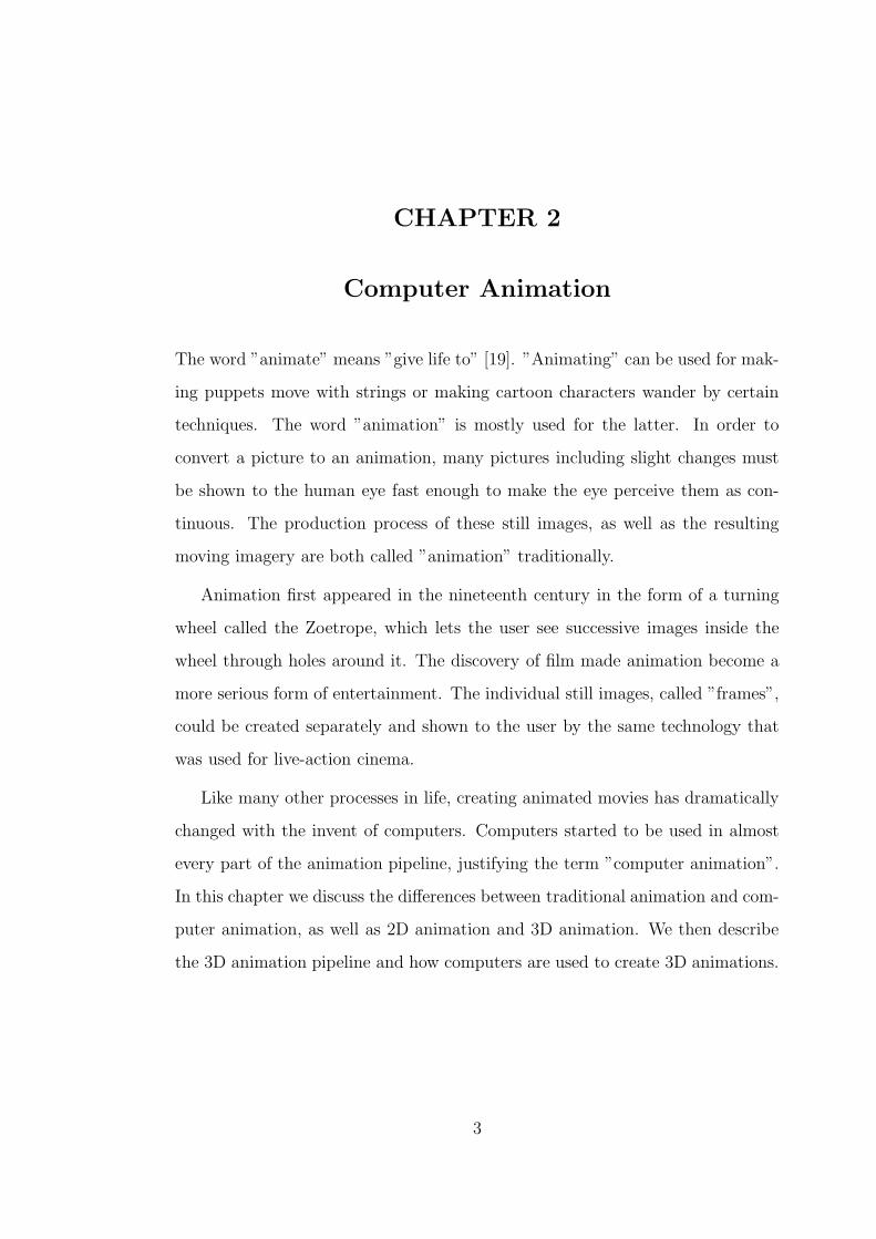
The most preferred modeling method is polygonal modeling. As seen in figure 2.1,

the primitives that polygonal models are defined by are, flat surfaces, straight

edges and vertices. Usually it is more efficient to represent polygonal models

as triangular meshes by triangulating the surfaces. This technique is simple

and intuitive for modelers because it simplifies the modeling process to defining

arbitrary vertex points in space. The complexity of the model is determined by

the number of vertices used.

Polygonal modeling is very useful for objects containing straight edges and

surfaces. As the complexity and the number of round surfaces increase, more

and more vertices need to be used in the model. Creating and managing high

number of vertices can be a very demanding task and there are a number of

modeling techniques that ease this process. Subdivision surfaces [6] is a useful

technique that iteratively approximates the B-spline surface defined by the input

6

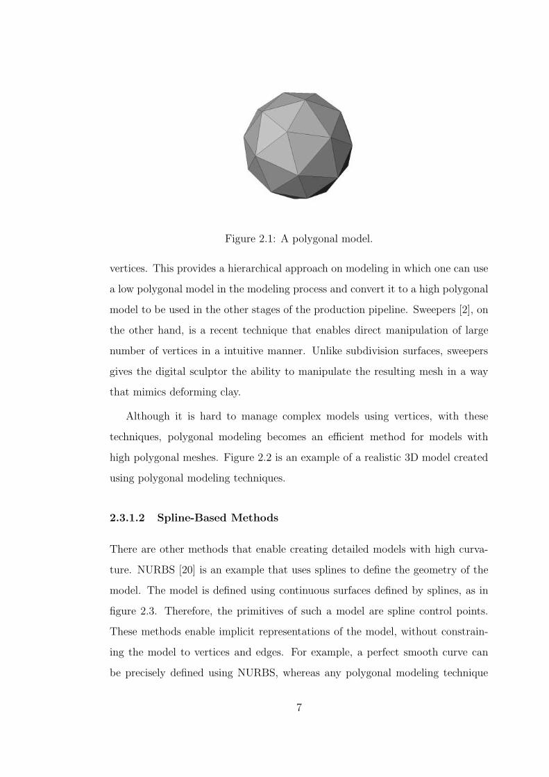
Figure 2.1: A polygonal model.

vertices. This provides a hierarchical approach on modeling in which one can use

a low polygonal model in the modeling process and convert it to a high polygonal

model to be used in the other stages of the production pipeline. Sweepers [2], on

the other hand, is a recent technique that enables direct manipulation of large

number of vertices in a intuitive manner. Unlike subdivision surfaces, sweepers

gives the digital sculptor the ability to manipulate the resulting mesh in a way

that mimics deforming clay.

Although it is hard to manage complex models using vertices, with these

techniques, polygonal modeling becomes an efficient method for models with

high polygonal meshes. Figure 2.2 is an example of a realistic 3D model created

using polygonal modeling techniques.

2.3.1.2 Spline-Based Methods

There are other methods that enable creating detailed models with high curva-

ture. NURBS [20] is an example that uses splines to define the geometry of the

model. The model is defined using continuous surfaces defined by splines, as in

figure 2.3. Therefore, the primitives of such a model are spline control points.

These methods enable implicit representations of the model, without constrain-

ing the model to vertices and edges. For example, a perfect smooth curve can

be precisely defined using NURBS, whereas any polygonal modeling technique

7

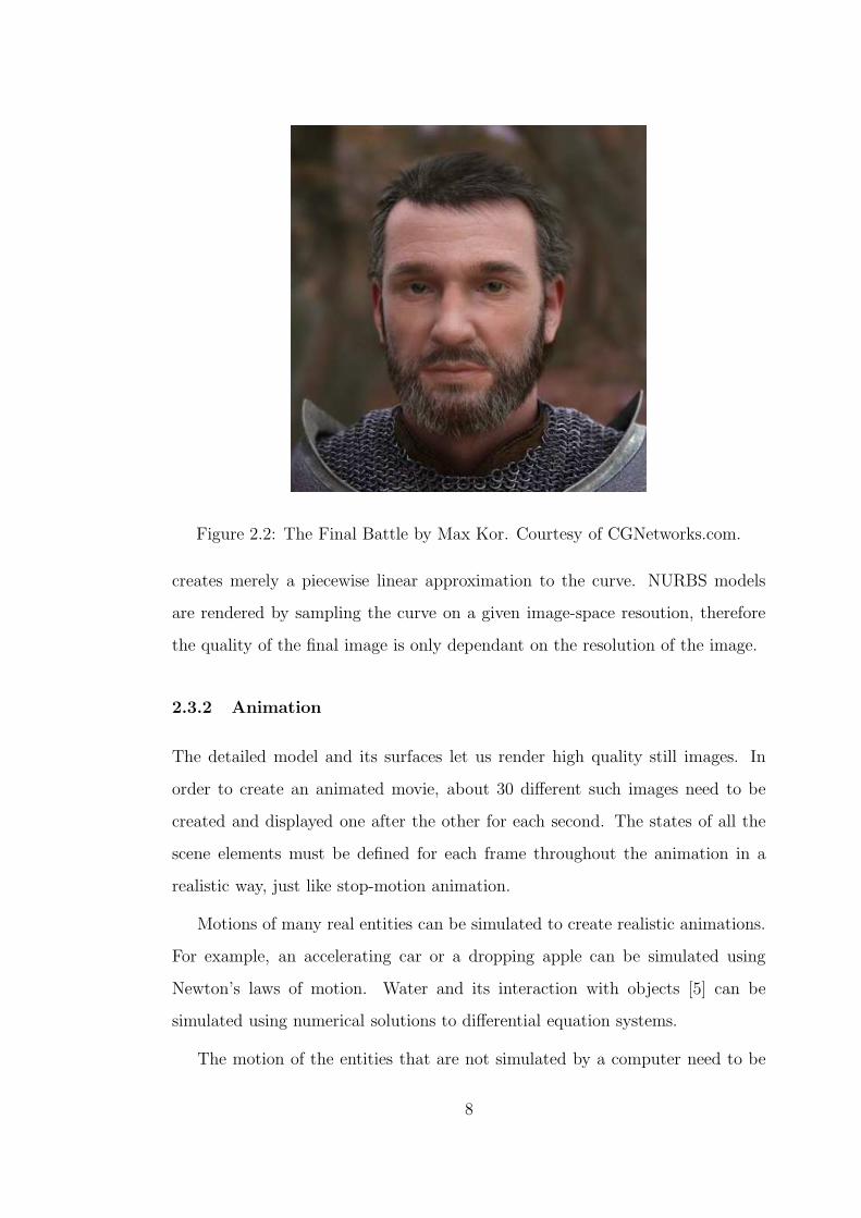
Figure 2.2: The Final Battle by Max Kor. Courtesy of CGNetworks.com.

creates merely a piecewise linear approximation to the curve. NURBS models

are rendered by sampling the curve on a given image-space resoution, therefore

the quality of the final image is only dependant on the resolution of the image.

2.3.2 Animation

The detailed model and its surfaces let us render high quality still images. In

order to create an animated movie, about 30 different such images need to be

created and displayed one after the other for each second. The states of all the

scene elements must be defined for each frame throughout the animation in a

realistic way, just like stop-motion animation.

Motions of many real entities can be simulated to create realistic animations.

For example, an accelerating car or a dropping apple can be simulated using

Newton’s laws of motion. Water and its interaction with objects [5] can be

simulated using numerical solutions to differential equation systems.

The motion of the entities that are not simulated by a computer need to be

8

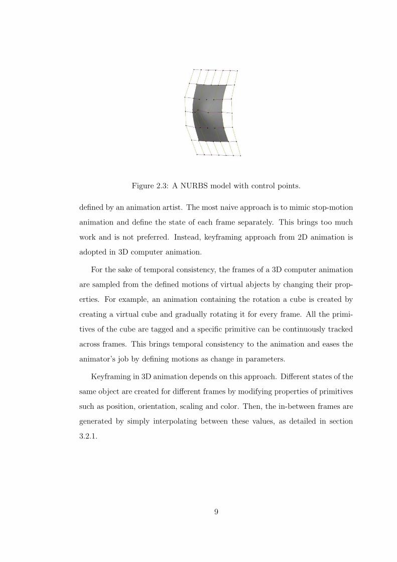
Figure 2.3: A NURBS model with control points.

defined by an animation artist. The most naive approach is to mimic stop-motion

animation and define the state of each frame separately. This brings too much

work and is not preferred. Instead, keyframing approach from 2D animation is

adopted in 3D computer animation.

For the sake of temporal consistency, the frames of a 3D computer animation

are sampled from the defined motions of virtual abjects by changing their prop-

erties. For example, an animation containing the rotation a cube is created by

creating a virtual cube and gradually rotating it for every frame. All the primi-

tives of the cube are tagged and a specific primitive can be continuously tracked

across frames. This brings temporal consistency to the animation and eases the

animator’s job by defining motions as change in parameters.

Keyframing in 3D animation depends on this approach. Different states of the

same object are created for different frames by modifying properties of primitives

such as position, orientation, scaling and color. Then, the in-between frames are

generated by simply interpolating between these values, as detailed in section

3.2.1.

9

2.3.3 Rendering

The animation created by the animator is sampled in discrete time steps to

create frames to be shown successively in the resulting animated movie, just like

taking photographs in a stop-mation animation. ”Rendering” is the process of

converting the 3D scene to a 2D image, similar to taking a virtual photograph.

In its simple definition, it requires the projection of 3D geometry into a 2D plane.

This is straightforward for simple points in space, but not all points are projected

as a simple point to the 2D plane. The projected image takes into account the

color and material of the point in space, how it is located relative to light sources,

whether it has other properties than just reflecting light, etc. In this respect, the

way the rendering algorithms create the final image determines the quality of the

resulting image.

The projection of a surface on the image has to convey the structure of the

surface in the space. Shadows and reflectance are real life properties of light

and object interaction and are simulated in rendering by lighting calculations.

Textures are 2D images mapped on a surface and they help creation realistic

images along with lighting.

10

CHAPTER 3

Full Body Character Animation

Creating three dimensional animations for complex entities is not an easy goal.

The tasks to be carried out in all the steps of the animation pipeline highly

depend on the complexity of the entity. As the entity gets more detailed, modeling

involves more work to be done, resulting with a model including higher number

of polygons. Animating such complex entities is also hard since the number of

parts that can move increases as the entity gets more complex. The animator

needs to consider all of these moving parts and create believeable animations for

them. The way that complex entities move is also usually complex. Constant

velocities and linear paths are usually not acceptable and there are implicit limits

on motion.

Human body is the most frequently used subject in computer animations and

it is a good example for a complex entity. There are 206 bones and 360 joints

in an adult human skeleton that all have special movement patterns. To cre-

ate a believable animation, the animator needs to simulate the movements of a

fair amount of these bones and joints. The H-Anim 200x specification in [10]

considers a humanoid figure with 14 joints to have a ”low level of articulation”,

compared to a figure with 72 joints, which is considered to have a ”high level of ar-

ticulation”. Some of these joints (e.g. shoulders) have crucial importance, where

others (e.g. vertebral joints) have less importance in the resulting animation.

The amount of joints considered affects the quality of the resulting animation as

well as the detail of generated motions.

Apart from joints and bones, there are many other factors that determine

quality of the animation. These include static properties of the image such as

11

the quality of the 3D model and the way it is shaded and projected into an

image. In the following sections we analyze the factors that affect the realism of

an animation in detail.

3.1 Modeling

Regardless of the representation method for the model, realistic human mod-

els are detailed and are hard to create. For example, The Ultimate Human by

cgCharacter [7], one of the best human models in existence, contains 772,500

polygons. Although for most applications models with a lower level of detail is

sufficient, human models usually require a high number of primitives. The num-

ber of primitives in the model depend on the level of detail and the level of detail

determines the realism of the model.

3.1.1 Hierarchical Modeling

Human models include a high number of primitives as well as a high number

of deformable parts (i.e. joints). Manipulation of such complex models requires

systematic approaches rather than manipulation of each primitive separately. For

example, when the animator wants to raise the arm of the model, she must be

able to do it easily without caring about every single primitive that needs to

move and deform. This is achieved by partitioning the model into rigid parts, or

bones, that are connected with joints and therefore imposing a hierarchy on the

model. The joints in human body are mostly hinge or ball and socket joints and

can be represented as rotations.

Figure 3.1 shows a skeleton hierarchy of a leg where the bones thigh, calf and

foot are connected by the joints knee and ankle. The bone thigh is the highest

bone in this hierarchy and foot is the lowest. The joints impose constraints on

this hierarchy and the movement of thigh automatically affects calf and foot. In

its simplest form, the bones that are lower in the hierarchy live in the coordinate

12

Calf

Ankle Foot

Knee

Thigh

Figure 3.1: A simple skeleton hierarchy of a leg.

frames that are defined by the bones that are higher in the hierarchy. The

geometric primitives that define the leg live in the coordinate frames of the bones

that they belong to. This way, the rotation of a joint higher in the hierarchy

automatically displaces the bones that are lower in the hierarchy and thus the

primitives are also displaced accordingly.

The ISO/IEC FCD 19774 - Humanoid animation (H-Anim) [10] is a standard

that defines a scalable framework for articulated humanoid models. Although

H-Anim defines joints and segments as separate entities, in practice, joints and

segments are usually merged into one structure called bones for the simplicity

in representation. Bones can be thought of as a hierarchy of segments in which

the connections implicitly define the joints. Since there are no closed chain kine-

matic structures on the human body, this representation does not introduce any

ambiguity. Figure 3.2 is an example of such a representation. Human characters

usually have the torso of the character as the root bone in the hierarchy.

Using a hierarchical model, different states of the complex model can be rep-

resented with a smaller number of parameters. This not only provides ease in

animating, but also ensures a consistency in the overall animation. If we have a

13

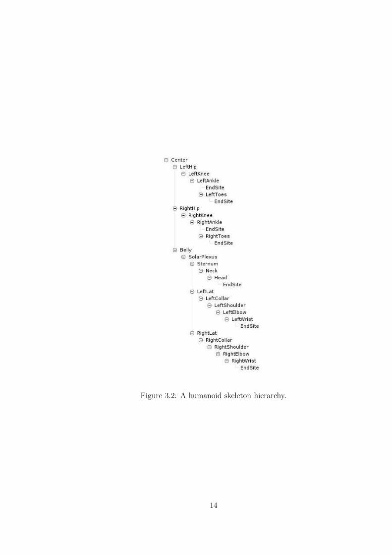
Figure 3.2: A humanoid skeleton hierarchy.

14

humanoid character with a model that has n+ 1 bones including the root bone,

we can define a configuration of the character as,

m(t) = (pr(t),qr(t),q1(t), . . . ,qn(t)) (3.1)

where pr(t) is the position of the root bone, qr(t) is the orientation of the

root bone and q1(t) . . .qn(t) are the orientations of the rest of the n bones in

hierarchy relative to the coordinate systems of their parents at time t. Using the

original hierarchical model and the configuration vector m(t), the state of the

model can be defined without any ambiguity.

A motion clip is defined as the configuration function m(t) as given in 3.1,

which is defined for an interval (ti, tf). For the movie clip to be played, the

character’s configurations between ti and tf must be displayed at the right time.

Note that m(t) defines the absolute position and orientation of the character’s

2D orientation in the xz-plane (i.e. floor plane). If all of the configurations that

define the motion clip are transformed in the xz-plane, the resulting motion clip

is also valid [14].

m′(ti) = Txz(x0, z0)Ry(θ0)m(ti) (3.2)

Where Txz(x0, z0) is a translation in the xz-plane by (x0, z0) and Ry(θ0) is a

rotation around y axis by θ0.

Although equation 3.2 generates a valid movie clip, it is not intuitive because

m(ti) is not necessarily in the origin of the xz-plane and the rotation Ry(θ0) will

also rotate the current displacement of m(ti) in the xz-plane. For this purpose,

it is intuitive to align one frame to origin, make the desired rotation and align it

back to the desired position, as in equation 3.4.

m(ti) = (pr(ti),qr(ti),q1(ti), . . . ,qn(ti)) (3.3)

m′(t) = Txz(x0, z0)Ry(θ0)Txz(−pr(ti))m(t) (3.4)

15

This approach enables us rotate the initial frame around itself with the angle

θ0 and position the character at (x0, z0) at the initial frame ti. Although it en-

ables enforcing the desired starting position of the character, it does not mention

exactly which way the character is facing. In addition to translating the initial

frame to origin, we can also make the character face the positive z axis at time

ti, which then allows us to explicitly define the orientation of the character. Note

that the character’s 2D orientation in the xz-plane solely depends on the 3D

orientation qr(t) of the root bone. We can rewrite qr(t) as three Euler angles in

zxy order as follows.

qr(t) = Ry(ψt)Rx(θt)Rz(φt) (3.5)

qr(t) = Ry(ψt)q0r(t) (3.6)

Therefore, we can rewrite the configuration of the character as follows.

m(t) = (pr(t),Ry(ψt)q0r(t),q1(t), . . . ,qn(t)) (3.7)

In order to start the motion clip at (x0, z0) with facing ψ0, we can apply the

following transformations to the motion clip.

m′(t) = Txz(x0, z0)Ry(ψ0)Ry(−ψti)Txz(−pr(ti))m(t) (3.8)

Where m(t) is as defined in equation 3.7. Then, equation 3.8 becomes

m′(t) = (Txz(x0, z0),Ry(ψ0)q0r(t),q1(t), . . . ,qn(t)) (3.9)

This representation gives us the freedom to explicitly set the position and

orientation of the character in xz-plane. We will use this representation for

interpolation in section 3.2.

16

3.2 Animation

The process of human animation is the focus of this thesis. Motions of many

real entities can be simulated to create realistic animations. On the other hand,

human motion is too complex to be modeled with equations since it needs to

obey the complex system of the human body as well as the laws of physics. The

physical properties of the human body such as muscles can be simulated, but

how the brain makes the muscles work is not easy to model because it depends

on many criteria that are beyond the scope of this thesis.

The general approach is to recreate human motion by either skilled animators

or by real motion data. Fortunately, animators do not have to specify the state of

the human body explicitly in each and every frame. Rather, a high level control

over a group of frames is created using hierarchical models, as detailed in section

3.1.1.

3.2.1 Keyframing

The word ”keyframing” has been an animation term since the early days of

animation. In 2D animation studios, a master artist would draw the important

frames that are enough to understand the animation. These frames are called

the keyframes. Afterwards, less skilled artists would draw the frames in between.

These frames are also called the in-betweens, and they fill in the motion defined

by keyframes [19]. The keyframes that serve as the important frames would

be enough to convey the overall motion and the in-betweens would merely be

transitions between them.

With the advent of 3D computer animation, the in-betweening approach be-

came a more concrete method. In 3D animation, the primitives corresponding to

the scene and the objects are all tagged and a state of the scene can be defined by

changing the properties of these primitives. Keyframes correspond to important

states of the scene that are defined by the parameters. Then, the in-between

17

frames are created using an interpolation function over the parameters that de-

fine the state of the scene and object primitives. This approach is also referred

to as parametric keyframing [25]. The parameters can be properties like position,

orientation, color, etc.

As explained in section 3.1.1, hierarchical approaches decrease the number of

parameters that are required to define the state of the model. In its simple form,

we can represent the state of a humanoid character as in equation 3.1, which is

as follows.

m(t) = (pr(t),qr(t),q1(t), . . . ,qn(t)) (3.10)

where pr(t) is the position of the root bone, qr(t) is the orientation of the

root bone and q1(t) . . .qn(t) are the orientations of the rest of the n bones in

hierarchy relative to the coordinate systems of their parents at time t.

In practice, the continuous functions in 3.10 are not explicitly defined. In

keyframing approach, the function values for a number of discrete values of t are

given and other values in between need to be computed using interpolation.

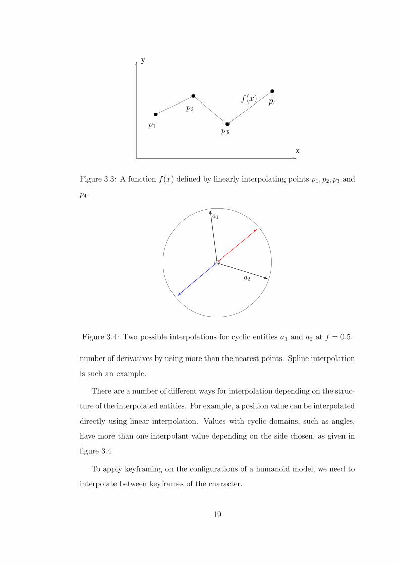
Interpolation can be defined as

inter(ai, ai+1, f) = ai+f (3.11)

where 0 ≤ f ≤ 1 is the fraction of interpolation. When f = 0, ai+f = ai and

when f = 1, ai+f = ai+1. The rest of the values are ”in between” ai and ai+1, as

shown in figure 3.3.

There are different ways for defining the interpolation function. Linear inter-

polation is the simplest interpolation technique and it is defined as follows.

lerp(ai, ai+1, f) = (1 − f)ai + fai+1 (3.12)

Although linear interpolation is intuitive, it does not provide continuity of

derivatives. There are other techniques that provide continuity up to a given

18

y

x

p1

p2

p3

p4f(x)

Figure 3.3: A function f(x) defined by linearly interpolating points p1, p2, p3 and

p4.

a1

a2

Figure 3.4: Two possible interpolations for cyclic entities a1 and a2 at f = 0.5.

number of derivatives by using more than the nearest points. Spline interpolation

is such an example.

There are a number of different ways for interpolation depending on the struc-

ture of the interpolated entities. For example, a position value can be interpolated

directly using linear interpolation. Values with cyclic domains, such as angles,

have more than one interpolant value depending on the side chosen, as given in

figure 3.4

To apply keyframing on the configurations of a humanoid model, we need to

interpolate between keyframes of the character.

19

m(t) = inter

(

m(ti),m(ti+1),t− titi+1 − ti

)

(3.13)

inter

(

m(ti),m(ti+1),t− titi+1 − ti

)

= (pr(t),qr(t),q1(t), . . . ,qn(t)) (3.14)

pr(t) = inter

(

pr(ti),pr(ti+1),t− titi+1 − ti

)

(3.15)

qr(t) = inter

(

qr(ti),qr(ti+1),t− titi+1 − ti

)

(3.16)

qk(t) = inter

(

qk(ti),qk(ti+1),t− titi+1 − ti

)

(3.17)

where ti ≤ t ≤ ti+1.

The interpolation function, inter, is required to interpolate between one po-

sition and n+1 orientation values that make up m(t), as in equations 3.13, 3.14,

3.15, 3.16, 3.17. Since the interpolation is done between static entities, the result

must be well defined. There are different techniques for interpolating between

these different entities and we discuss a number of possible techniques in the

following sections.

3.2.1.1 Interpolation of 3D Translations

A translation T in 3D consists of three parameters (x, y, z) that define the trans-

lation about the three axes, therefore a translation can be represented by a vector.

T (t) =

x(t)

y(t)

z(t)

(3.18)

Interpolation techniques such as linear interpolation or spline interpolation

can directly be applied to these parameters to create the inbetween values. If we

know T (ti) and T (ti+1), we can find T (t) for ti ≤ t ≤ ti+1 as follows.

20

x(t)

y(t)

z(t)

=

inter(

x(ti), x(ti+1),t−ti

ti+1−ti

)

inter(

y(ti), y(ti+1),t−ti

ti+1−ti

)

inter(

z(ti), z(ti+1),t−ti

ti+1−ti

)

(3.19)

For the interpolation function, we can use any kind of interpolation technique

depending on the application needs. Linear interpolation is the simplest technique

but it does not provide continuity of derivatives and produces unnatural results.

Spline interpolation is a better choice and it is the favorite interpolation technique

for keyframe animations.

3.2.1.2 Interpolation of 3D Rotations

Unlike translations, rotations require more attention for interpolation. In 2D,

we can represent rotations just by one angle and as shown in figure 3.4, there

can be more than one choices as the result of interpolation. In 3D, it gets more

complicated because not only there can be more than one cyclic parameters,

but also there are more than one representations of the same 3D rotation and

interpolation of these different representations create potentially different results.

Euler angles is the most naive representation for a rotation in 3D. Any rotation

in 3D can be represented as three consecutive rotations around the coordinate

axes. Thus, a rotation R can be represented as the composition of three rotations

R1, R2, R3 [16].

R = R1R2R3 (3.20)

The rotation axes corresponding to R1, R2 and R3 can be chosen arbitrarily.

One of the most common rotation orders in literature is the xyz order, which is

also called pitch-roll-yaw. The angles (φ, θ, ψ) are used to represent the rotations

around x, y and z axes in order.

An interpolation for R(t) can be written as follows.

21

R(t) = R1(t)R2(t)R3(t) (3.21)

R1(t) = inter

(

R1(ti),R1(ti+1),t− titi+1 − ti

)

(3.22)

R2(t) = inter

(

R2(ti),R2(ti+1),t− titi+1 − ti

)

(3.23)

R3(t) = inter

(

R3(ti),R3(ti+1),t− titi+1 − ti

)

(3.24)

The interpolations are carried out on the angle values as follows.

φ(t) = inter

(

φ(ti), φ(ti+1) + kφ2π,t− titi+1 − ti

)

(3.25)

θ(t) = inter

(

θ(ti), θ(ti+1) + kθ2π,t− titi+1 − ti

)

(3.26)

ψ(t) = inter

(

ψ(ti), ψ(ti+1) + kψ2π,t− titi+1 − ti

)

(3.27)

where kφ, kθ and kψ are adjusted to choose the side of interpolation as shown

in 3.4. For the interpolation function, linear interpolation or spline interpolation

can be used, spline interpolation creating smoother results.

There are a number of drawbacks in using Euler angles for interpolation.

First of all, Euler angles are prone to the gimbal lock problem [24]. When θ is

90 degrees in an xyz order of rotation, x and z axes are aligned over each other

and they affect the resulting rotation exactly the same, and it is impossible to

make a rotation around the axis that is perpendicular to the current x and y axes

without changing θ. This results in the loss of one degree of freedom and is not

desireable.

Another major drawback of using Euler angles for interpolation is that Euler

angles are ambiguous. The very same 3D rotation may be represented by more

than one Euler angle values (φ, θ, ψ). If one of the interpolants has such a con-

dition, the resulting interpolation will be different for different (φ, θ, ψ) values of

the interpolant, although they represent the exact same rotation.

22

A better alternative for interpolating rotations is spherical linear interpolation

(slerp) using quaternions [24]. Quaternions are four dimensional mathematical

constructs that are similar to complex numbers. A quaternion q has a scalar and

a three dimensional vector part and can be written as,

q = (s,v) (3.28)

A rotation in 3D around a vector n by angle θ can be represented by a unit

quaternion as follows.

q = (cos(θ/2),n sin(θ/2)) (3.29)

A vector v can be represented with a quaternion p = (0,v). Rotation of

a vector v represented by a quaternion p, with the rotation represented by a

quaternion q is as follows [24].

p′ = qpq−1 (3.30)

Where q−1 is the multiplicative inverse of q and multiplication of quaternions

is defined as

q1q2 = (s1,v1).(s2,v2) = (s1s2 − v1.v2, s1v2 + s2v1 + v1 × v2) (3.31)

The inverse of a unit quaternion is equal to its conjugate which is defined as

q−1 = (s,−v) (3.32)

Using equation 3.30, we can rotate a vector with any rotation represented as

in equation 3.29. Note that all the quaternions on a line that passes through the

origin of the 4D quaternion space represent the same rotation [24]. All quater-

nions in this domain are unit quaternions and except directly opposite ones, no

23

q2

q1

q2

q1

lerp slerp

Figure 3.5: lerp vs slerp. Note the growing distances on the sphere in the middle

of lerp.

two quaternions represent the same rotation. Therefore, an interpolation done

in this domain is well defined and unique. Furthermore, unlike Euler angles,

quaternion representation of rotation does not suffer from gimbal lock.

One way of interpolating between unit quaternions is interpolating between

the quaternion parameters directly using lerp and projecting the interpolation

steps back on the unit sphere. Although this is a straightforward way, the inter-

polation tends to speed up in the middle. A better way is, doing the interpolation

on the surface of the sphere, which ensures constant speed, as seen in figure 3.5.

This interpolation technique is called spherical linear interpolation or slerp

[24], and is formulated by

slerp(q1, q2, t) =sin(1 − t)θ

sin θq1 +

sin tθ

sin θq2 (3.33)

where |q1| = |q2| = 1 and q1.q2 = cos θ.

slerp is shown to perform better than other methods for interpolating ro-

tations [24], and is the choice of rotation interpolation in character animation.

There are spline based methods [12] that guarantee higher order derivatives and

incremental methods [4] that enable efficient computation of slerp.

With lerp for the root bone position and slerp for bone orientations, keyframe

24

animation is a powerful tool in 3D animation.

Keyframing is a helpful tool for animators, but creating the keyframes and ad-

justing motions require a fair amount of time of the artist. Creating keyframed

animations for a long animated movie including many characters is still a de-

manding job. To address this problem there are a number of techniques given in

the next sections.

3.2.2 Physically Based Methods

Instead of considering humanoid models as simple geometric objects, physically

based methods aim to apply laws of physics to the model by enriching the model

with physical properties of the human body. With a human model that is aware

of the physical constraints such as Newton’s laws and joint torque constraints,

the human motion can be created with less input from the user.

Pure physical methods are more popular in robotics than in animation. In

[15], the authors create a computer model of a real humanoid robot and using

motion planning techniques they create motions that can also be used to control

the real robot. The motions created include simple motions like reaching and

grabbing as well as complex full body motions like locomotion in an environment

with obstacles.

Although pure physical methods enable the creation of humanoid motions

by using simple constraints, the created motions are often too ”mechanical” and

inhuman. Therefore pure physical methods are not preferred in computer anima-

tion. Nevertheless, combined with other methods it can be a powerful tool, as

detailed in section 3.2.4.1.

[9] is another example for creating physically valid human motions. In this

approach, a given simple human animation is iteratively converted to a physically

valid animation. This approach can be classified as a hybrid method of keyfram-

ing and physically based methods. As far as realism is concerned, this approach

creates better animations since the animator supplies an initial animation and

25

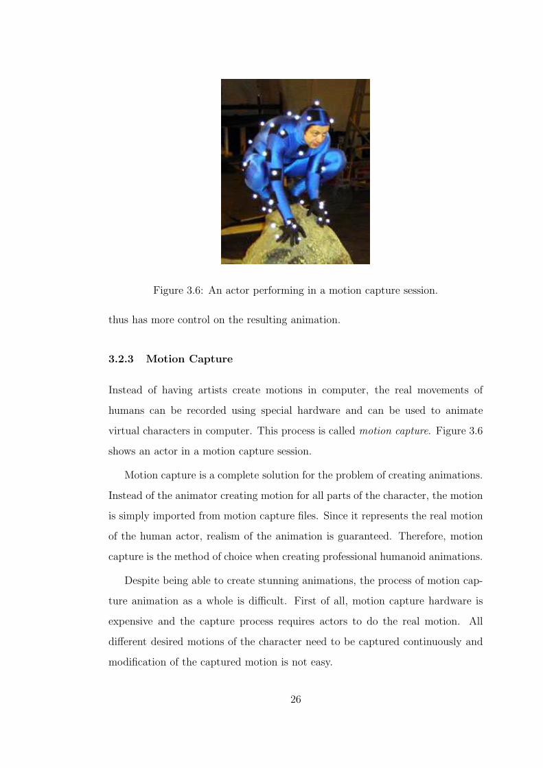
Figure 3.6: An actor performing in a motion capture session.

thus has more control on the resulting animation.

3.2.3 Motion Capture

Instead of having artists create motions in computer, the real movements of

humans can be recorded using special hardware and can be used to animate

virtual characters in computer. This process is called motion capture. Figure 3.6

shows an actor in a motion capture session.

Motion capture is a complete solution for the problem of creating animations.

Instead of the animator creating motion for all parts of the character, the motion

is simply imported from motion capture files. Since it represents the real motion

of the human actor, realism of the animation is guaranteed. Therefore, motion

capture is the method of choice when creating professional humanoid animations.

Despite being able to create stunning animations, the process of motion cap-

ture animation as a whole is difficult. First of all, motion capture hardware is

expensive and the capture process requires actors to do the real motion. All

different desired motions of the character need to be captured continuously and

modification of the captured motion is not easy.

26

Motion capture hardware captures positions and orientations of specific points

on the human body in discrete time intervals. These captured points are de-

termined by the placement of motion capture hardware on the actor’s body.

Therefore, the motion defined by the captured points is highly dependant on the

placement of motion capture sensors as well as the shape of the actor’s body

and it cannot be applied directly to a character with a different body shape. In

addition to all these problems, raw motion capture data includes noise that is

generated by the motion capture hardware.

In order to overcome these problems, raw motion capture data is modified

and converted into a more useable state by post processing. The noise is cleaned

and the motion is retargeted into a standard skeleton with bone hierarchy. The

resulting motion capture data that is used to drive the character is of the form

m(t) = (pr(t),qr(t),q1(t), . . . ,qn(t)) (3.34)

which is the same as equation 3.1. The motion function m(t) is defined in

discrete time intervals, usually 30 samples per second.

3.2.4 Motion Capture Based Methods

Although it can be a difficult task, motion capture is the best way to create

realistic human motions. The biggest problem with motion capture is that the

capture process needs to be repeated for every desired motion since manipulating

motion capture data is not easy. Many researchers have worked on the problem

of manipulating motion capture data while preserving its realism. These works

can be divided into two approaches: physically based and interpolation based.

Some researchers used the newly created motion capture data by one of these

two methods, and formed motion graphs in order to create a data structure that

will enable the creation of motions that are combinations of small motion clips.

These methods are given in the following sections.

27

3.2.4.1 Physically Based

As we have seen in section 3.2.2, physical properties of humans can be used to

create motions that abide user constraints as well as laws of physics. Motions that

are created from scratch are usually not realistic, but physically based motions

can be used to modify existing motions to make them more realistic. In [26],

motion capture data is modified by the user and balance constraints are used to

make the created motions physically valid. In [21], motion capture data is used to

create a model of human motion and that model is used to reconstruct motions

according to the user constraints and physical constraints.

In general, physical constraints are composed of static balance, dynamic bal-

ance, joint torque limits and minimum displaced mass. Static balance is obtained

by summing the forces and torques affecting to the character to zero. Although

static balance constraints are not satisfied in a moving character, they are useful

to create keyframes and statically stable trajectories that can be converted into

dynamically stable trajectories. Dynamic balance is a fuzzy concept and there

is no concrete definition to classify motions for dynamic stability. One good

approximation is keeping the zero moment point on the ground contact surface

[15]. This ensures that the character does not fall, but restricts it from perform-

ing more active motions, such as running. Different heuristics are also available,

but none of them give a consistent solution. Joint torque limits ensure that no

joint is overloaded with force than it normally can. Minimum displaced mass is a

heuristic used in motion reconstruction and it restricts the motion to be smooth.

Physically based motion generation using motion capture data is one of the

useful tools for creating transitions between two motion clips. We will see another

method in the next section, and in section 3.2.4.3, we describe the use of these

methods to create a motion graph.

28

y

x

f(x)

g(x)

x0 x1 x3x2

inter(

f(x), g(x), x−x0

x3−x0

)

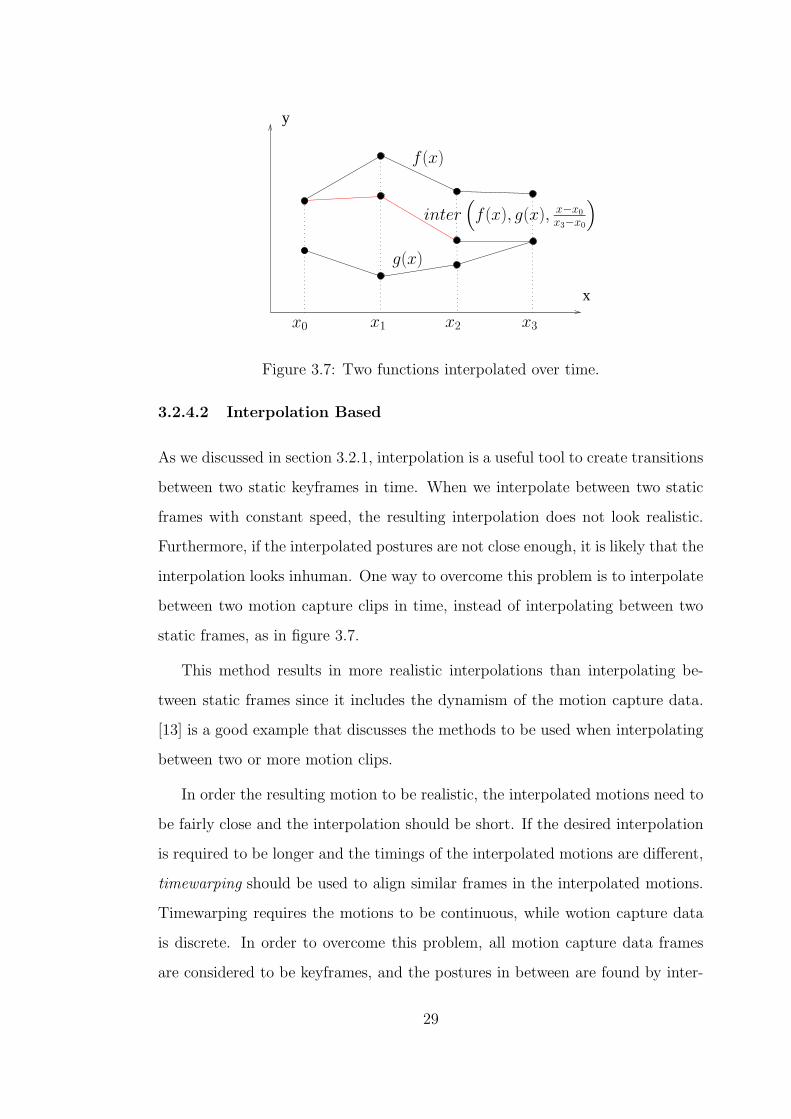
Figure 3.7: Two functions interpolated over time.

3.2.4.2 Interpolation Based

As we discussed in section 3.2.1, interpolation is a useful tool to create transitions

between two static keyframes in time. When we interpolate between two static

frames with constant speed, the resulting interpolation does not look realistic.

Furthermore, if the interpolated postures are not close enough, it is likely that the

interpolation looks inhuman. One way to overcome this problem is to interpolate

between two motion capture clips in time, instead of interpolating between two

static frames, as in figure 3.7.

This method results in more realistic interpolations than interpolating be-

tween static frames since it includes the dynamism of the motion capture data.

[13] is a good example that discusses the methods to be used when interpolating

between two or more motion clips.

In order the resulting motion to be realistic, the interpolated motions need to

be fairly close and the interpolation should be short. If the desired interpolation

is required to be longer and the timings of the interpolated motions are different,

timewarping should be used to align similar frames in the interpolated motions.

Timewarping requires the motions to be continuous, while wotion capture data

is discrete. In order to overcome this problem, all motion capture data frames

are considered to be keyframes, and the postures in between are found by inter-

29

x

y

g(x)

f(x)

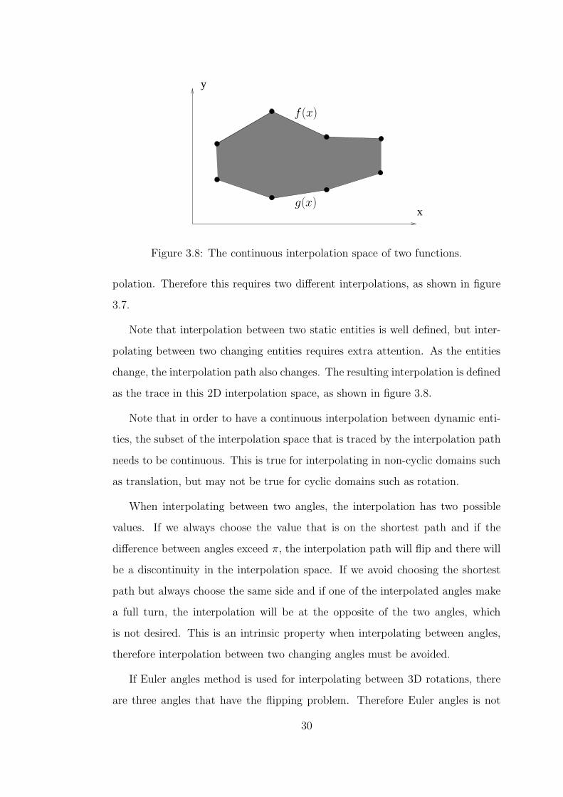
Figure 3.8: The continuous interpolation space of two functions.

polation. Therefore this requires two different interpolations, as shown in figure

3.7.

Note that interpolation between two static entities is well defined, but inter-

polating between two changing entities requires extra attention. As the entities

change, the interpolation path also changes. The resulting interpolation is defined

as the trace in this 2D interpolation space, as shown in figure 3.8.

Note that in order to have a continuous interpolation between dynamic enti-

ties, the subset of the interpolation space that is traced by the interpolation path

needs to be continuous. This is true for interpolating in non-cyclic domains such

as translation, but may not be true for cyclic domains such as rotation.

When interpolating between two angles, the interpolation has two possible

values. If we always choose the value that is on the shortest path and if the

difference between angles exceed π, the interpolation path will flip and there will

be a discontinuity in the interpolation space. If we avoid choosing the shortest

path but always choose the same side and if one of the interpolated angles make

a full turn, the interpolation will be at the opposite of the two angles, which

is not desired. This is an intrinsic property when interpolating between angles,

therefore interpolation between two changing angles must be avoided.

If Euler angles method is used for interpolating between 3D rotations, there

are three angles that have the flipping problem. Therefore Euler angles is not

30

InterpolationEdges

Similar Region

Clip 2

Clip 1

Figure 3.9: Creation of a motion graph using interpolation.

a good choice for interpolating between rotations. slerp using quaternions is a

better way since there are less chances of having a flip, i.e. the vector parts of

the quaternions have to get to the exact opposite poles of the unit sphere. Nev-

ertheless, if the quaternions are close to the opposite poles of the sphere, then

the middle point of the path will move much faster than the interpolated quater-

nions themselves, creating possible discontinuities. Therefore, choosing motion

clips that are close enough to each other ensures continuity in interpolation.

3.2.4.3 Motion Graphs

The techniques explained in sections 3.2.4.1 and 3.2.4.2 can be used to create

transitions between motion capture clips. Apart from being local solutions, such

transitions can be used to create a larger data structure containing all the movie

clips in the database and possible transitions between them. This data structure

is called a motion graph, was introduced by [3] and [14]. [3] considers graph nodes

as motion clips and [14] considers edges as motion clips. Both approaches have

their advantages and disadvantages, but the latter approach has been preferred

by more researchers and is more intuitive.

Assume we have two motion clips in our database, and we find a region in

these clips that have similar frames. By using physically based or interpolation

based methods, we can create transitions between these motion clips, as in figure

3.9.

These interpolations enable us start playing motion clip A, and using the

interpolation from A to B, continue with playing motion clip B. This powerful

31

construct, when applied to a large scale motion clip database, enables creation of

a motion graph. A motion graph is a directed graph G = (V,E) having motion

clips on its edges, E, and nodes in V connect the clips that can be played after

each other. Any traversal on this graph creates a valid string of motion clips and

the traversal can be constrained for specific purposes in order to create motions

that obey user constraints. The work that we present in this thesis also adopts a

motion graph approach, as detailed in chapter 5.

3.3 Rendering

The importance of rendering depends on the type of animated movie to be cre-

ated. If the created movie is a simple animation, basic rendering properties like

colored surfaces and simple lights will be sufficient. If the movie is intended to

look realistic as in figure 2.2, the rendering part of the animation pipeline becomes

more important. Elements of rendering such as lights and surface properties are

vital for an animation to look realistic. Realistic human models require detailed

surface properties. The skin should not be perfectly flat and homogeneous, the

hair needs to look like it is really made of many tiny hairs, eyes need to look

wet and reflective and clothes need to look like real fabric. Rendering is the final

polish on the animated movie and can give a professional look to the movie. The

detail of rendering process greatly affects the realism of the final image, therefore

in order to create a quality movie, rendering should not be overlooked.

32

CHAPTER 4

Character Navigation

Automating the character navigation process requires systematic approaches to

be taken. Using a motion graph we can create different paths, but we need to

be able to guide the graph traversal in order not to have exponential running

times dominated by trial and error. This guidance can be used for determining

the path to take and trying to approximate that path by graph traversals in the

motion graph. Fortunately, motion planning, which is a branch of robotics, deals

with this problem of path planning that will enable us find the path to follow

before moving our character.

4.1 Motion Planning

The problem of motion planning deals with finding a set of control commands for

a robot structure in order to make it carry out a certain task. The problem can

be generalized to finding a sequence of control commands to take a robot from an

initial state to a goal state. More formally [17], the problem is finding a series of

configurations q1,q2, . . . ,qn that will take the robot A in the workspace W, from

the initial configuration qinit to the goal configuration qgoal. A configuration of

the robot is defined as the variable properties of the robot that are relevant to

the motion planning task. The configuration space, or the C-Space, C of the

robot A is defined as all possible configurations that the robot may be in.

A path from qinit to qgoal in C-Space is defined as a continuous map τ :

[0, 1] → C with τ(0) = qinit and τ(1) = qgoal.

The region of W occupied by A when the robot is in configuration q is repre-

33

setned by A(q). The regions of the configuration space that are not feasible are

called configuration space obstacles or C-Obstacles that correspond to obstacle

regions B in W, and are defined as

CB = {q|A(q) ∩ B 6= ∅} (4.1)

The notation of configuration space simplifies the problem from motion plan-

ning for a robot to path planning, but possibly in a higher dimensional space.

A path found in the configuration space represents a motion trajectory for the

robot in the workspace.

There are a number of motion planning algorithms that operate by finding a

path in C-Space. Two fundamental probabilistic algorithms, PRM and RRT,

are given in the next sections.

4.1.1 PRM

Probabilistic roadmap method (PRM) [11] is the most popular probabilistic motion

planning algorithm. It runs in two phases, a learning phase and a query phase.

The main idea behind PRM is to construct a roadmap of the environment in the

learning phase, and to find the shortest path on that graph in the query phase.

The learning phase is a long process that requires the discovery of most of the

environment and the query phase enables fast queries on the precomputed graph.

The goal of the learning phase is to form a roadmap R = (N,E) that contains

the connectivity of the environment. The nodes N represent a set of probabilis-

tically selected configurations and the edges E represent possible simple paths

between these configurations. The nodes are selected using a probabilistic ap-

proach and connected by edges using a local planner using k-nearest neighbors

as shown in figure 4.1. The local planner is usually a simple planner like straight

line or A*.

The aim of the query phase is finding a path from an initial configuration qinit

34

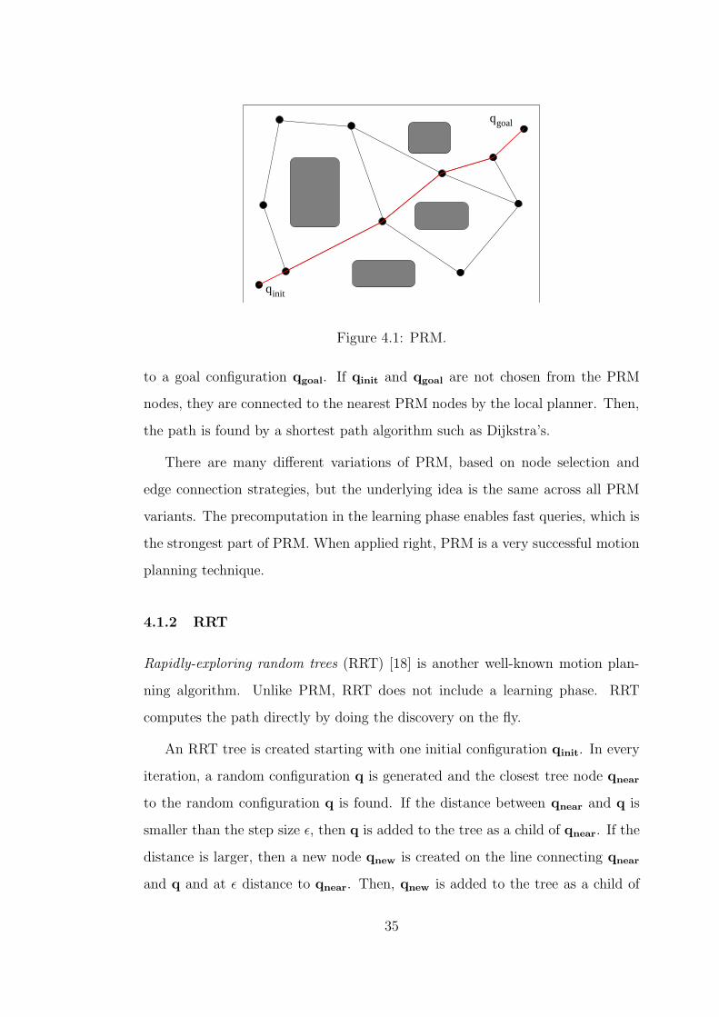
qinit

qgoal

Figure 4.1: PRM.

to a goal configuration qgoal. If qinit and qgoal are not chosen from the PRM

nodes, they are connected to the nearest PRM nodes by the local planner. Then,

the path is found by a shortest path algorithm such as Dijkstra’s.

There are many different variations of PRM, based on node selection and

edge connection strategies, but the underlying idea is the same across all PRM

variants. The precomputation in the learning phase enables fast queries, which is

the strongest part of PRM. When applied right, PRM is a very successful motion

planning technique.

4.1.2 RRT

Rapidly-exploring random trees (RRT) [18] is another well-known motion plan-

ning algorithm. Unlike PRM, RRT does not include a learning phase. RRT

computes the path directly by doing the discovery on the fly.

An RRT tree is created starting with one initial configuration qinit. In every

iteration, a random configuration q is generated and the closest tree node qnear

to the random configuration q is found. If the distance between qnear and q is

smaller than the step size ε, then q is added to the tree as a child of qnear. If the

distance is larger, then a new node qnew is created on the line connecting qnear

and q and at ε distance to qnear. Then, qnew is added to the tree as a child of

35

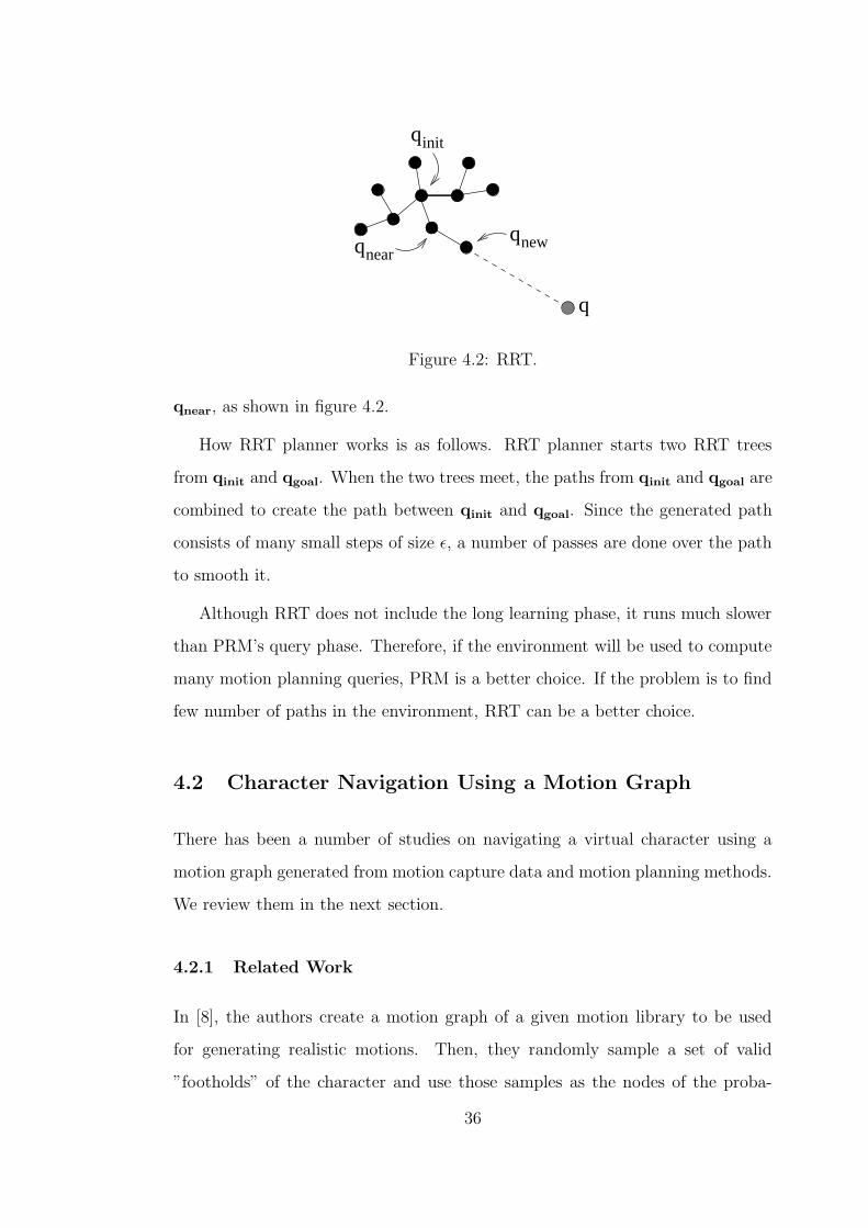
qinit

qnearqnew

q

Figure 4.2: RRT.

qnear, as shown in figure 4.2.

How RRT planner works is as follows. RRT planner starts two RRT trees

from qinit and qgoal. When the two trees meet, the paths from qinit and qgoal are

combined to create the path between qinit and qgoal. Since the generated path

consists of many small steps of size ε, a number of passes are done over the path

to smooth it.

Although RRT does not include the long learning phase, it runs much slower

than PRM’s query phase. Therefore, if the environment will be used to compute

many motion planning queries, PRM is a better choice. If the problem is to find

few number of paths in the environment, RRT can be a better choice.

4.2 Character Navigation Using a Motion Graph

There has been a number of studies on navigating a virtual character using a

motion graph generated from motion capture data and motion planning methods.

We review them in the next section.

4.2.1 Related Work

In [8], the authors create a motion graph of a given motion library to be used

for generating realistic motions. Then, they randomly sample a set of valid

”footholds” of the character and use those samples as the nodes of the proba-

36

bilistic roadmap algorithm. Then, the connection of these nodes are done using

the motion capture data. Since the motion capture frame entering to a node must

be compatible with the frame that is exiting it, the creation of the roadmap is

constrained by the motion capture data. The authors stretch the motions to fit

the random footholds as necessary, and create an embedded roadmap of walking

motions. Then, the queries are done on this roadmap just as in the original PRM.

In [23] the authors take a similar approach and create a motion graph. Then,

they discretize the workspace and find connections between motion clips starting

from the discrete cells in the workspace. As in [8], the motions are stretched

as necessary to fit the cells. Then, the motion graph is embedded into these

discrete cells. The graph created by these cells correspond to the roadmap of the

environment. In the query phase, they traverse this graph to find a path that

will take the character from the initial position to the goal position.

4.2.2 Our Approach

The two approaches reviewed in section 4.2.1 are successful techniques that en-

able fast queries once the roadmaps are set. They include a long learning phase in

which the roadmaps are formed by embedding the motion graph to the environ-

ment and finding and modifying motion clips to connect these roadmap nodes.

One property of both approaches is that they require a long learning phase and

the size of the embedded graphs depend on the size of the environment. This

property makes these methods hard to scale. This is not a problem in small

settings, but in large settings like multi-level games, the motion graph needs to

be embedded to all the maps in the game, causing extra preprocessing and stor-

age. Another drawback is that they include stretching of motions in the roadmap

generation, which means they may find a path with a stretched motion where a

unedited motion would do just fine. Embedding the motion graph also constrains

the motions that can be used, prohibiting satisfaction of runtime constraints that

could be satisfied by using a different motion clip than the one in the graph.

37

In our approach to this problem, we do not embed the motion graph on the

environment. We create a basic PRM roadmap of the environment and make our

queries on that roadmap to find a possible path between start and goal. Then we

traverse the motion graph on the fly to reach subgoals defined on the chosen path.

This way, the user is free to put runtime constraints on the planned motion. The

details of our method is given in chapter 5.

38

CHAPTER 5

Proposed Solution

In this chapter, we discuss the problem that we address and propose a solution

based on the related work that we discussed in previous chapters.

5.1 Problem

The problem that we are interested is automatically creation of human character

animation navigating from an initial position to a goal position in an environment

with obstacles. We want the system to enable the user to create obstacles and

set a start and a goal position in a virtual environment. Then, we want the

system to automatically generate a realistic walking animation that makes the

character walk from the initial position to the goal position, without colliding

with obstacles.

5.2 Solution

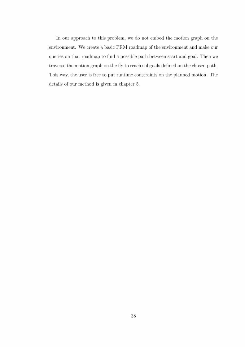
We created a system with a graphical user interface that lets the user place obsta-

cles, the start and the goal positions and creates an animation. The components

of our system is described in figure 5.1.

Inputs to the system are the motion capture data and the environment. The

motion analyzer module reads the motion capture library and creates a motion

graph, as a preprocessing step. The environment, with the initial and goal posi-

tions are given by the user to the planning module via the user interface. The

planning module first finds a collision-free path in the environment from the ini-

39

MotionPlanner

MotionAnalyzer

Path Planner

Motion CaptureData

Environment Subgoals

Motion Graph

Animation

Figure 5.1: Components of our system.

tial to the goal position. Then, it creates evenly distributed checkpoints on this

path that will be the subgoals. Using this path as a guide, the planning module

starts traversing on the motion graph to reach the subgoals one by one. After the

goal is reached, the corresponding graph traversal is converted to motion data

and is displayed to the user.

5.3 Motion Graph

As explained in chapter 3, creating character animations from scratch is difficult

and using existing motion capture data is a preferred method for creating new

motions. We adopt this approach and we use public domain stock motion cap-

ture data provided by University of Southern California, Institute for Creative

Technologies. The motion capture library includes straight and curved walking

motions of a human subject, which is suitable for creating animations of character

navigation. The motion capture data is in Biovision hierarchical format(BVH),

which includes a hierarchical skeleton and the configuration of the character for

each frame. The configuration is given in the following format.

m(t) = (pr(t),qr(t),q1(t), . . . ,qn(t)) (5.1)

where pr(t) is the position of the root bone, qr(t) is the orientation of the root

bone and q1(t) . . .qn(t) are the orientations of the rest of the n bones in hierarchy

relative to the coordinate systems of their parents at time t. All orientations are

40

free 3D rotations since BVH format does not include any specific constraints for

joints.

We create a motion graph from the input motions in order to create custom

animations. The motion graph data structure is introduced in section 3.2.4.3. We

use interpolation to connect the separate motion clips. The analysis of motion

capture data and creation of the motion graph are costly operations since every

frame in the motion library must be compared to every other frame. Therefore,

this step is performed offline as a preprocessing step and saved to the disk to be

used later.

Now we describe the motion graph creation process in detail.

5.3.1 The Distance Metric

In order to consider similarities between frames, we need a distance metric be-

tween frames of motion capture data. We use a distance metric similar to the

metric introduced by [14]. Using the configuration of character m(t), we can

find absolute positions of the body parts as a vector p(t). The distance metric

is defined over these position values. We define the distance between two frames

as the weighted sum of squared distances of the corresponding body parts. We

include two frames before and after the corresponding frames in order to capture

derivative information [14]. The distance metric is given in equation 5.2

D(ti, tj) =2∑

d=−2

n∑

k=1

wk|pk(ti+d) − pk(tj+d)|2 (5.2)

where wk is the weight for the kth body part and pk(t) is the kth element of

the vector p(t). Two body postures with the weighted distances are shown in

figure 5.2.

This distance metric allows us to find frames of motion capture data that are

close to each other for making interpolations.

41

Figure 5.2: Calculation of our distance metric. Note that the bones in the hand

are not included to prevent them from dominating the result.

(c)(b)(a)

Figure 5.3: (a) A similarity image of a motion capture data with itself. (b)

Regions lower than threshold. (c) Selected interpolation regions.

5.3.2 Finding Interpolation Regions

Using the distance metric, we find the similarity for all possible frame pairs in

the library. Figure 5.3(a) shows a similarity matrix between two motion files in

our motion library, represented by an intensity map. Darker regions correspond

to lower values.

We apply a threshold τ on the similarity matrices and find the regions that

have similarity values lower than τ , as shown in figure 5.3(b). Then we find re-

gions of length l that are under the threshold, as in figure 5.3(c). These regions

42

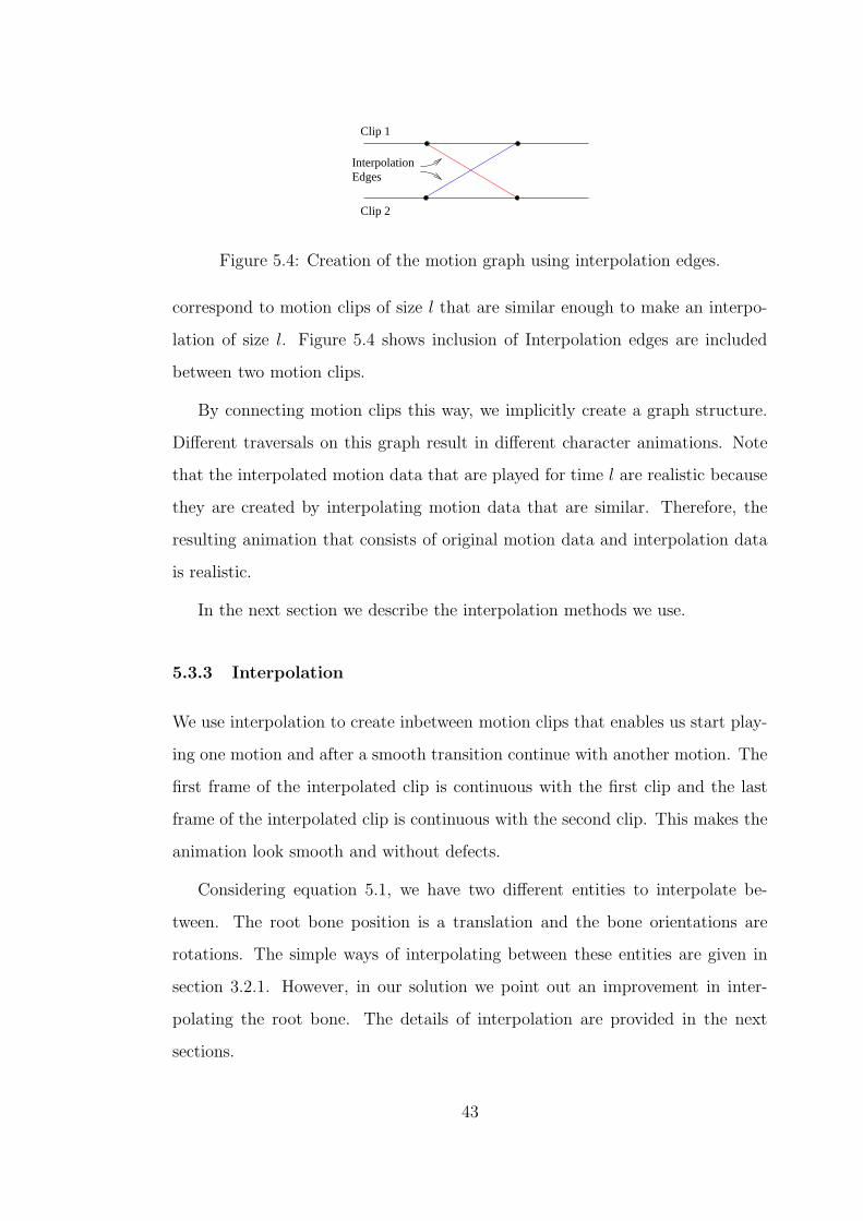
InterpolationEdges

Clip 1

Clip 2

Figure 5.4: Creation of the motion graph using interpolation edges.

correspond to motion clips of size l that are similar enough to make an interpo-

lation of size l. Figure 5.4 shows inclusion of Interpolation edges are included

between two motion clips.

By connecting motion clips this way, we implicitly create a graph structure.

Different traversals on this graph result in different character animations. Note

that the interpolated motion data that are played for time l are realistic because

they are created by interpolating motion data that are similar. Therefore, the

resulting animation that consists of original motion data and interpolation data

is realistic.

In the next section we describe the interpolation methods we use.

5.3.3 Interpolation

We use interpolation to create inbetween motion clips that enables us start play-

ing one motion and after a smooth transition continue with another motion. The

first frame of the interpolated clip is continuous with the first clip and the last

frame of the interpolated clip is continuous with the second clip. This makes the

animation look smooth and without defects.

Considering equation 5.1, we have two different entities to interpolate be-

tween. The root bone position is a translation and the bone orientations are

rotations. The simple ways of interpolating between these entities are given in

section 3.2.1. However, in our solution we point out an improvement in inter-

polating the root bone. The details of interpolation are provided in the next

sections.

43

Path for clip 2

Path

for

clip

1

Figure 5.5: Trajectory obtained by directly interpolating root bone parameters.

5.3.3.1 Interpolation of Position and Orientation of the Root Bone

The root bone is a special bone that is the parent of all the bones in the character

hierarchy. Therefore, the absolute position of the body depends on the placement

of the root bone and the direction the character’s torso faces depends on the

orientation of the root bone. The position of the root bone, pr(t), is a translation

from the origin and the orientation of the root bone, qr(t), is a 3D rotation. The

naive way of making an interpolation between these entities is to interpolate the

position and orientation separately. Although this seems like a good approach,

it has a drawback when doing long interpolations. The interpolated positions

of the rootbone in the two clips create a trajectory that the character takes in

the interpolated movie. In some examples, as given in figure 5.5 the created

trajectory may require the character to move in an unnatural way. Therefore,

directly interpolating between the positions and orientations of the root bone is

not the correct approach.

This problem has also been pointed out in [13] and the proposed solution is to

interpolate between the changes in the position and orientation of the root bone.

The motivation behind this approach is as follows. The character’s position and

44

orientation in the global frame depends on its initial state and the changes that

are introduced by the frames that have been played so far. The change in the

character’s position and orientation depends on the actions of the character that

are represented by the frames played. For example, when frames including step-

ping forwards are played, the character’s position changes towards the direction

that the character is facing. When a frame including stepping right is played,

the character’s position and orientation change accordingly. If we blend these

motions together, we expect the character to change its trajectory between these

two changes. Therefore, interpolating between changes of the character’s position

and orientation should give a better result than interpolating the position and

orientation separately.

For this purpose, we modify the motion representation given in equation 5.1

as follows

m(t) = (pr(t),Ry(ψt)q0r(t),q1(t), . . . ,qn(t)) (5.3)

where pr(t) is the position of the root bone, Ry(−ψt) is the rotation that

would make the model face the positive z axis, q0r(t) is the orientation of the root

bone and q1(t) . . .qn(t) are the orientations of the rest of the n bones relative to

the coordinate systems of their parents at time t. Note that Ry(ψt)q0r(t) = qr(t)

and the character’s 2D orientation in the xz-plane solely depends on pr(t) and

Ry(ψt).

For the sake of simplicity, we rewrite the motion representation as follows

m(t) = (c(t),q0r(t),q1(t), . . . ,qn(t)) (5.4)

where c(t) = (pr(t),Ry(ψt)) corresponds to the position and orientation of

the character.

This representation allows handling the interpolation of the character’s posi-

tion and orientation separate from the full body posture. The position and orien-

45

tation of the character’s absolute values are not important since they depend on

the initial position and orientation. On the other hand, the absolute values of the

joint orientations, including the root bone’s orientation except Ry(ψt), are im-

portant since they define the body posture. Therefore, when interpolating we can

consider the relative values of Ry(ψt) and q0r(t), but not of qi(t) for i = 1, . . . , n.

Another benefit of this representation is that it decouples the navigation prob-

lem from the motion capture data. Therefore we can use only c(t) alone to plan

the path of the character, which is simpler than considering the entire pose.

According to this, we define differential root bone interpolation as follows.

c(t) = c(tl) + lerp

(

(

c(t1u) − c(t1l ))

,(

c(t2u) − c(t2l ))

,t− titf − ti

)

t− tlδ

(5.5)

where

tku =⌈

t

δ

⌉

(5.6)

δk =δ

tf − ti(5.7)

for k = 1, 2.

In equation 5.5, subtraction of c(t) and multiplication with a scalar is used.

They are defined straightforwardly as follows

c(t1) − c(t2) = (pr(t1) − pr(t2),Ry(ψt1 − ψt2)) (5.8)

kc(t) = (kpr(t),Ry(kψt)) (5.9)

Figure 5.6 summarizes this interpolation process.

Figure 5.7 shows the paths taken by standard linear interpolation and dif-

ferential linear interpolation. The path taken in (a) makes the character slide

sideways, whereas the path in (b) is realistic.

46

∆c(t2)

∆c(t)

∆c(t1)

Figure 5.6: Trajectory obtained by differentially interpolating position and ori-

entation of the character.

Path for clip 2

Path

for

clip

1

basicdifferential

Figure 5.7: Basic interpolation vs differential interpolation.

47

Note that the two interpolated movie clips can be of different lengths and have

different δk’s. This technique is generic and any interpolation technique such as

linear interpolation or spline interpolation can be used in place of inter. In our

implementation we use linear interpolation for the interpolation function.

One thing to consider about differential interpolation is that the interpolation

must be defined over a unit interval δ. The resulting interpolation is still defined

as a continuous function of time, but the interval δ is a parameter that defines

the interpolation uniquely. When δ → 0, the two interpolated transformations

are done ”at the same time”, as detailed in [1].

5.3.3.2 Interpolation of Joint Orientations

As discussed in the previous chapter, character position and orientation are rela-

tive values and a whole motion clip can be translated or rotated in the floor plane

without distorting the motion in any way. On the other hand, orientations of the

bones in the skeleton hierarchy are absolute values and any arbitrary change in

their values lead to entirely different body postures. Therefore, a differential

interpolation approach is neither necessary nor useful.

Although it is more straightforward to interpolate bone orientations, there

are a number of important points to consider. As explained in 3.2.1, there are a

number of different methods for making interpolation between 3D rotations. As

long as the interpolated body postures are similar enough, slerp is a convenient

method. However, the interpolation we consider for creating the motion graph is

different than the one in 3.2.1 in the sense that there are two changing entities

to be interpolated between. As discussed in 3.2.4.2, the resulting interpolation is

likely to have discontinuities if the interpolated clips are not similar. This is not

a problem in our implementation since we choose similar regions of motion clips

for interpolation.

Interpolation of the orientation of one bone is carried out as follows

48

qk(t) = slerp(qk(t1),qk(t

2),t− titf − ti

) (5.10)

Using equation 5.5 and 5.10, the interpolation is uniquely defined.

5.3.4 Creation of the Motion Graph

The way we create the motion graph is as follows. Using the distance metric given

in section 5.3.1, we find the similarity matrices between all motion clips. Then, we

apply a threshold τ and find regions of size l that are under the threshold. Then

we calculate interpolations between these regions and form the motion graph.

We prune the end sites of the motion graph in order to make sure that it does

not have any dead ends.

The creation of the graph is a computationally expensive process, so it is done

once and saved to the disk for later use.

5.4 Planning the Path

In runtime, after loading the previously generated motion graph, the user is

enabled to create an environment and make path queries for the character. The

details of these processes are detailed in the upcoming sections.

5.4.0.1 Environment

The user is presented with an environment editing system where the user can

define a 2D map of the environment. The user can set the width and height

of a rectangular area, and create rectangular obstacles with various sizes. The

obstacles are assumed to be prismatic, starting from the ground and tall enough

that the character cannot climb on. Although we use simple obstacles, this

method can be used for complex interactions with obstacles if appropriate motion

capture data is available.

49

Figure 5.8: The character represented by a cylinder in the environment.

After creating the environment, the user sets a start and an end point. The

goal of the system is to find a walking motion from the given start to the goal.

5.4.0.2 Path Planning

The first step in planning the character’s motion is to find a feasible path from

the start to the goal. For this purpose we use PRM [11], which is explained in

4.1.1.

The character is assumed to be a robot with the shape of a cylinder, for

the sake of simplicity in collision detection. In the 2D environment map, the

character is represented with a circle, as in figure 5.8.

The radius r is determined so that the cylinder contains the whole body of

the character in various motions.

With these assumptions, the problem becomes planning a path for a circular

robot in a 2D environment. We find the C-Space by growing the obstacles by r

and use PRM to find the path as in figure 5.9.

We generate n randomly distributed nodes and connect the k nearest neigh-

bors. Then, using Dijkstra’s algorithm, we find the shortest path between start

and goal. The resulting path is the guide for the character to follow, as shown in

figure 5.10.

50

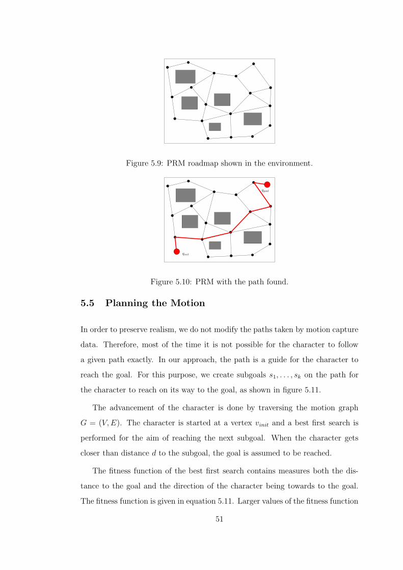
Figure 5.9: PRM roadmap shown in the environment.

qinit

qgoal

Figure 5.10: PRM with the path found.

5.5 Planning the Motion

In order to preserve realism, we do not modify the paths taken by motion capture

data. Therefore, most of the time it is not possible for the character to follow

a given path exactly. In our approach, the path is a guide for the character to

reach the goal. For this purpose, we create subgoals s1, . . . , sk on the path for

the character to reach on its way to the goal, as shown in figure 5.11.

The advancement of the character is done by traversing the motion graph

G = (V,E). The character is started at a vertex vinit and a best first search is

performed for the aim of reaching the next subgoal. When the character gets

closer than distance d to the subgoal, the goal is assumed to be reached.

The fitness function of the best first search contains measures both the dis-

tance to the goal and the direction of the character being towards to the goal.

The fitness function is given in equation 5.11. Larger values of the fitness function

51

qinit

qgoal

Figure 5.11: Subgoals on the path.

means worse states.

fit(t) = (2 − cosα(t))d(t) (5.11)

Where d is the distance to target and α is the angle that the orientation of

the character makes with the straight line between the character and the target.

Therefore, if the character is directed straight towards to the goal, f(x) = d. If

the character faces opposite direction from the goal, f(x) = 3d. We chose this

fitness function in order to promote making the character go straight to the target

and making the character walk straight is easier than making it manuever.

This method is summarized in algorithms 5.5.1 and 5.5.2.

Using this traversal, the subgoals are reached one by one and the motion

Algorithm 5.5.1 Find path(G = (V,E), (s1, . . . , sk), d)

1: path = ∅

2: subpath = ∅

3: t = 1

4: while t < k do

5: subpath = traverse(G, end(path), st, d)

6: path = path + subpath

7: t = t + 1

8: return path

52

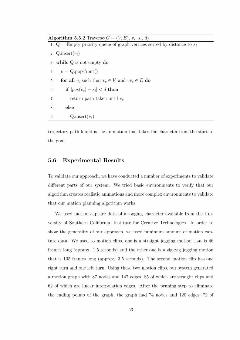
Algorithm 5.5.2 Traverse(G = (V,E), vi, si, d)

1: Q = Empty priority queue of graph vertices sorted by distance to si

2: Q.insert(vi)

3: while Q is not empty do

4: v = Q.pop-front()

5: for all vc such that vc ∈ V and vvc ∈ E do

6: if |pos(vc) − si| < d then

7: return path taken until vc

8: else

9: Q.insert(vc)

trajectory path found is the animation that takes the character from the start to

the goal.

5.6 Experimental Results

To validate our approach, we have conducted a number of experiments to validate

different parts of our system. We tried basic environments to verify that our

algorithm creates realistic animations and more complex environments to validate

that our mation planning algorithm works.

We used motion capture data of a jogging character available from the Uni-

versity of Southern California, Institute for Creative Technologies. In order to

show the generality of our approach, we used minimum amount of motion cap-

ture data. We used to motion clips, one is a straight jogging motion that is 46

frames long (approx. 1.5 seconds) and the other one is a zig-zag jogging motion

that is 105 frames long (approx. 3.5 seconds). The second motion clip has one

right turn and one left turn. Using these two motion clips, our system generated

a motion graph with 87 nodes and 147 edges, 85 of which are straight clips and

62 of which are linear interpolation edges. After the pruning step to eliminate

the ending points of the graph, the graph had 74 nodes and 120 edges, 72 of

53

which are straight clips and 48 of which are linear interpolation edges. We used

13 frames as the length of linear interpolations.

We showed that our system can use such small amounts of motion capture

data to generate long and complex motions. To show that the generated motion

data is realistic, we set up a simple environment with one obstacle and made the

character go around it to reach the goal, as seen in figures 5.12 a - d.

a b

c d

Figure 5.12: Simple environment.

In order to show that our algorithm creates complex motions for navigation

in a labyrinth, we set up a larcer scale environment with more obstacles. The

path planning algorithm successfully found a path as in figures 5.13 a -d, and

the motion planning algorithm successully traversed the motion graph and found

a suitable motion trajectory that passes through the subgoals to reach the goal,

as in 5.14 a - d. The accompanying videos also contain the resulting motions of

these two different cases.

The running times of our algorithm in simple cases were instantaneous, while

some of the complex casestook a longer time to complete. To explore the efficiency

54

a b

c d

Figure 5.13: Complex environment PRM screenshots.

of our algorithm, we prepared 6 complex environments and ran our algorithm for

them. The running times and the resulting animation times are shown in table

5.1.

Note that the graph generation phase takes a longer time than the querying

phase, but since it is preprocessing and it will not affect the use of this algorithm,

it is acceptable. The fast running times of our algorithm make it suitable for real-

Empty Map 1 Map 2 Map 3 Map 4 Map 5 Map 6 Map 7

Running time 0.004 2.651 4.991 0.118 0.272 0.021 0.028 0.136

Length 21.6 63.01 46.1 44.5 44.93 30.5 35.97 52.57

Table 5.1: Running times for different environments.

55

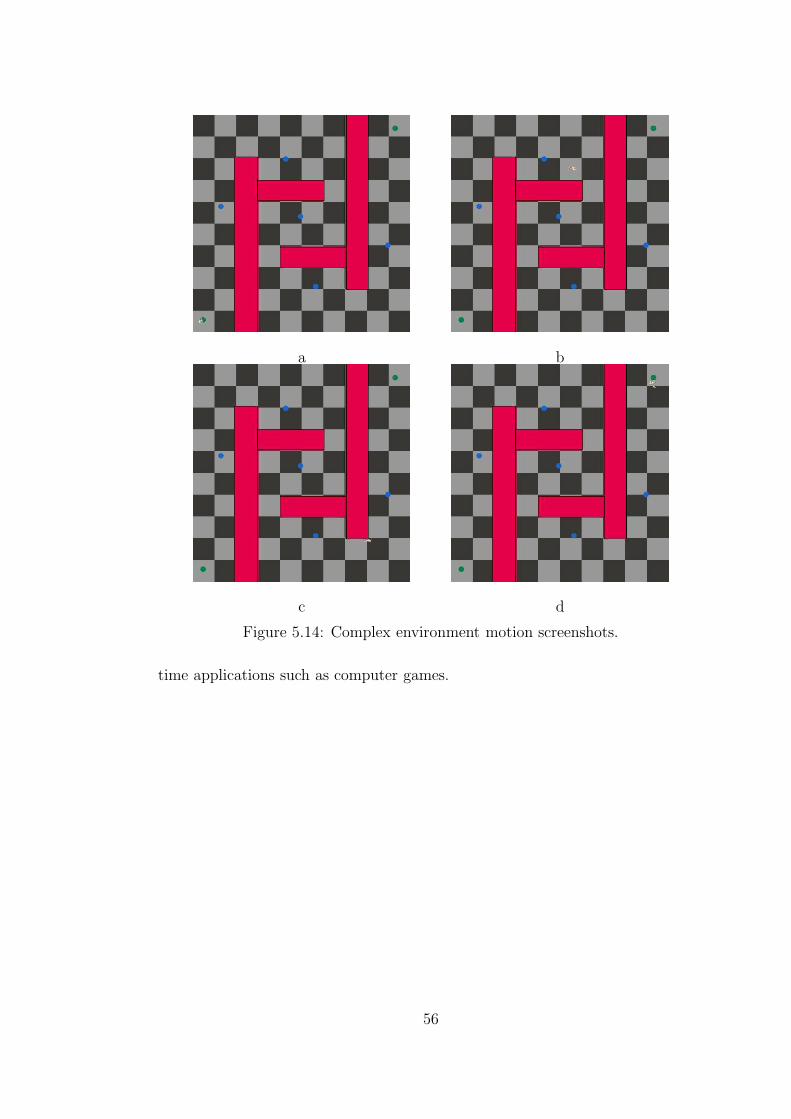
a b

c d

Figure 5.14: Complex environment motion screenshots.

time applications such as computer games.

56

CHAPTER 6

Conclusion

In this study, we presented a method for automatically generating realistic walk-

ing animations from a start position to a goal position in an environment with

obstacles. We reviewed current metods for animation and compared different

methods available. We described the use of motion capture data and different

ways of modifying it, along with a comparison of different interpolation tech-

niques. We identified problems that occur when interpolating the root bone, and

gave a detailed solution using differential interpolation. Using interpolation, we

described the creation of a motion graph, a useful data structure for creating

sequences of motions.

The runtime performance of the technique we presented depends on the path

planning and motion planning approaches, and the our experiments show the

efficiency of the approaches we used. This algorithm can be used for real-time

and interactive applications such as computer games. The only preprocessing

done is to create the motion graph, and it is possible to change our system to

enable addition of new motion capture data by constructing the graph incremen-

tally. It is also possible to extend this approach to moving obstacles with known

trajectories using corresponding extensions to prm.

This system can be used in computer games, movies or any other application

that requires a variety of human animations, dramatically easing the animator’s

job. Our future work includes the creation of an interactive avatar control system

and planning motions with behaviors using appropriate motion data.

57

References

[1] Marc Alexa. Linear combination of transformations. In SIGGRAPH ’02:Proceedings of the 29th annual conference on Computer graphics and inter-active techniques, pages 380–387, New York, NY, USA, 2002. ACM Press.

[2] Alexis Angelidis, Geoff Wyvill, and Marie-Paule Cani. Sweepers: Sweptuser-defined tools for modeling by deformation. In SMI ’04: Proceedings ofthe Shape Modeling International 2004 (SMI’04), pages 63–73, Washington,DC, USA, 2004. IEEE Computer Society.

[3] Okan Arikan, David A. Forsyth, and James F. O’Brien. Motion synthesisfrom annotations. ACM Trans. Graph., 22(3):402–408, 2003.

[4] Tony Barrera, Anders Hast, and Ewert Bengtsson. Incremental sphericallinear interpolation. In SIGRAD 2004: Special theme - Environmental visu-alization, Linkping electronic conference proceedings, pages 7–10. LinkpingUniversity Electronic Press, 2004.

[5] Mark Carlson, Peter J. Mucha, and Greg Turk. Rigid fluid: animating theinterplay between rigid bodies and fluid. ACM Trans. Graph., 23(3):377–384, 2004.

[6] E. Catmull and J. Clark. Recursively generated b-spline surfaces on arbitrarytopological meshes. In Seminal graphics: poineering efforts that shaped thefield, pages 183–188, New York, NY, USA, 1998. ACM Press.

[7] cgCharacter Software. http://www.cgcharacter.com.

[8] Min Gyu Choi, Jehee Lee, and Sung Yong Shin. Planning biped locomotionusing motion capture data and probabilistic roadmaps. ACM Trans. Graph.,22(2):182–203, 2003.

[9] Anthony C. Fang and Nancy S. Pollard. Efficient synthesis of physicallyvalid human motion. ACM Trans. Graph., 22(3):417–426, 2003.

[10] ISO/IEC FCD 19774 - humanoid animation (H-Anim). http://www.h-anim.org/Specifications/H-Anim200x.

[11] Lydia Kavraki, Petr Svestka, Jean-Claude Latombe, and Mark H. Overmars.Probabilistic roadmaps for path planning in high-dimensional configurationspaces. IEEE Trans. Robotics Automation, 12(4):566–580, August 1996.

[12] Myoung-Jun Kim, Myung-Soo Kim, and Sung Yong Shin. A general con-struction scheme for unit quaternion curves with simple high order deriva-tives. In SIGGRAPH ’95: Proceedings of the 22nd annual conference onComputer graphics and interactive techniques, pages 369–376, New York,NY, USA, 1995. ACM Press.

58

[13] Lucas Kovar and Michael Gleicher. Flexible automatic motion blendingwith registration curves. In SCA ’03: Proceedings of the 2003 ACM SIG-GRAPH/Eurographics Symposium on Computer animation, pages 214–224,Aire-la-Ville, Switzerland, Switzerland, 2003. Eurographics Association.

[14] Lucas Kovar, Michael Gleicher, and Frederic Pighin. Motion graphs. InSIGGRAPH ’02: Proceedings of the 29th annual conference on Computergraphics and interactive techniques, pages 473–482, New York, NY, USA,2002. ACM Press.

[15] James Kuffner, Koichi Nishiwaki, Satoshi Kagami, Masayuki Inaba, andHirochika Inoue. Dynamically-stable motion planning for humanoid robots.Autonomous Robots (special issue on Humanoid Robotics), 12:105–118, 2002.

[16] Jack B. Kuipers. Quaternions and Rotation Sequences : A Primer withApplications to Orbits, Aerospace and Virtual Reality. Princeton UniversityPress, 2002.

[17] Jean-Claude Latombe. Robot Motion Planning. Kluwer Academic Publish-ers, Boston, MA, 1991.

[18] Steven LaValle and James Kuffner. Rapidly-Exploring Random Trees:Progress and Prospects. In Proc. Int. Workshop on Algorithmic Founda-tions of Robotics (WAFR), pages SA45–SA59, 2000.

[19] Michael O’Rourke. Principles of Three-Dimensional Computer Animation:Modeling, Rendering, and Animating with 3d Computer Graphics. W. W.Norton & Co., Inc., New York, NY, USA, 1998.

[20] Les Piegl. On NURBS: a survey. IEEE Comput. Graph. Appl., 11(1):55–71,1991.

[21] Zoran Popovic and Andrew Witkin. Physically based motion transforma-tion. In SIGGRAPH ’99: Proceedings of the 26th annual conference onComputer graphics and interactive techniques, pages 11–20, New York, NY,USA, 1999. ACM Press/Addison-Wesley Publishing Co.

[22] William T. Reeves. Inbetweening for computer animation utilizing movingpoint constraints. In SIGGRAPH ’81: Proceedings of the 8th annual confer-ence on Computer graphics and interactive techniques, pages 263–269, NewYork, NY, USA, 1981. ACM Press.

[23] Paul S. A. Reitsma and Nancy S. Pollard. Evaluating motion graphs forcharacter navigation. In SCA ’04: Proceedings of the 2004 ACM SIG-GRAPH/Eurographics symposium on Computer animation, pages 89–98,New York, NY, USA, 2004. ACM Press.

[24] Ken Shoemake. Animating rotation with quaternion curves. In SIGGRAPH’85: Proceedings of the 12th annual conference on Computer graphics andinteractive techniques, pages 245–254, New York, NY, USA, 1985. ACMPress.

59

[25] Scott N. Steketee and Norman I. Badler. Parametric keyframe interpolationincorporating kinetic adjustment and phrasing control. In SIGGRAPH ’85:Proceedings of the 12th annual conference on Computer graphics and inter-active techniques, pages 255–262, New York, NY, USA, 1985. ACM Press.

[26] Victor Brian Zordan and Jessica K. Hodgins. Motion capture-driven sim-ulations that hit and react. In SCA ’02: Proceedings of the 2002 ACMSIGGRAPH/Eurographics symposium on Computer animation, pages 89–96, New York, NY, USA, 2002. ACM Press.

60