a–ne feedback policies for robust control with...
TRANSCRIPT

Affine Feedback Policies forRobust Control with Constraints
Paul James Goulart
Churchill College
Control GroupDepartment of EngineeringUniversity of Cambridge
A dissertation submitted for the degree of
Doctor of Philosophy
November 3, 2006Revised January 16, 2007


Abstract
This thesis is concerned with the optimal control of linear discrete-time systems with convexstate and input constraints and subject to bounded disturbances. It is shown that thenonconvex problem of finding a constraint admissible affine state feedback policy over afinite horizon can be converted to an equivalent convex problem, where the input at eachtime is modelled as an affine function of prior disturbances. This implies that a broad classof constrained finite horizon robust and optimal control problems can be solved efficientlyusing convex optimization methods. These policies can be then used in the design of robustreceding horizon control (RHC) laws such that the system constraints are satisfied for alltime and for all allowable disturbance sequences.
By choosing a control policy from this class that minimizes the expected value of a quadraticfunction of the states and inputs at each time, it is possible to provide sufficient conditionsunder which the policy optimization problem is convex at each time step, and for which suchan RHC control law renders the closed-loop system input-to-state stable. Alternatively,using a quadratic cost function where the disturbance is negatively weighted as in H∞
control, one can provide conditions under which the finite-horizon min-max control problemto be solved at each time step can be rendered convex-concave, and provide conditionsguaranteeing that the `2 gain of the resulting closed-loop system is bounded.
When all of the system constraints are linear, the complexity of solving these problems growspolynomially with the problem size for a wide variety of disturbance classes, making theirsolution tractable using standard techniques in convex optimization. In the particular casethat the cost function is a quadratic function of the states and inputs and the disturbanceset is ∞-norm bounded, a sparse problem structure can be recovered via introduction ofstate-like variables and decomposition of the problem into a set of coupled finite horizoncontrol problems. This decomposed problem can then be formulated as a highly structuredquadratic program, solvable by a primal-dual interior-point method for which each iterationrequires a number of operations that increases cubicly with horizon length.
Finally, it is shown how the ideas presented can be extended to the output feedback case. Asimilar convex reparameterization is applied to the problem of finding a constraint admissi-ble affine output feedback policy over a finite horizon, to be used in conjunction with a fixedlinear state observer. A time-invariant control law is developed using these policies thatcan be computed by solving a finite-dimensional, tractable optimization problem at eachtime step, and that guarantees that the closed-loop system satisfies the system constraintsfor all time.


Acknowledgements
I would like to thank Professor Jan Maciejowski for his support and guidance as my super-visor throughout my research. I am also greatly indebted to Dr. Eric Kerrigan for his help,advice and mentoring over the past three years; much of the work in this dissertation is theproduct of our collaboration during our mutual time in Cambridge.
I would also like to thank the members of the MPC group, and in particular Dr. DannyRalph for many helpful conversations and ideas. A further thanks to past and presentmembers of the Control Group for making my stay such an enjoyable one.
A special thanks is due to Theo Epstein for making it happen in 2004.
Generous financial support from the Gates Cambridge Trust, Churchill College and theDepartment of Engineering is gratefully acknowledged.
Finally, I would like to thank my family for their support, particularly my wife, Emma, forher constant love, patience and kindness.
Paul J. GoulartCambridge,November 3, 2006
i

ii
Declaration
As required by the University Statute, I hereby declare that this dissertation is not substan-tially the same as any that I have submitted for a degree or diploma or other qualificationat any other university. This dissertation is the result of my own work and includes nothingwhich is the outcome of work done in collaboration, except where specified explicitly in thetext.
I also declare that the length of this dissertation is less than 65,000 words and that thenumber of figures is less than 150.
Paul J. GoulartChurchill CollegeCambridgeNovember 3, 2006
iii

iv

Contents
Notation ix
1 Introduction 11.1 Background . . . . . . . . . . . . . . . . . . . . . . . . . . . . . . . . . . . . 11.2 Affine Feedback Policies . . . . . . . . . . . . . . . . . . . . . . . . . . . . . 31.3 Organization and Highlights . . . . . . . . . . . . . . . . . . . . . . . . . . . 5
2 Background 92.1 Convex Sets . . . . . . . . . . . . . . . . . . . . . . . . . . . . . . . . . . . . 9
2.1.1 Convex Hulls . . . . . . . . . . . . . . . . . . . . . . . . . . . . . . . 112.1.2 Operations on Convex Sets . . . . . . . . . . . . . . . . . . . . . . . 112.1.3 Polar Sets and Dual Cones . . . . . . . . . . . . . . . . . . . . . . . 13
2.2 Convex Functions . . . . . . . . . . . . . . . . . . . . . . . . . . . . . . . . . 152.2.1 Operations on Convex Functions . . . . . . . . . . . . . . . . . . . . 152.2.2 Support and Gauge Functions . . . . . . . . . . . . . . . . . . . . . . 16
2.3 Convex Optimization . . . . . . . . . . . . . . . . . . . . . . . . . . . . . . . 172.3.1 Linear and Quadratic Programs . . . . . . . . . . . . . . . . . . . . . 182.3.2 Second-Order Cone Programs . . . . . . . . . . . . . . . . . . . . . . 192.3.3 Linear Matrix Inequalities and Semidefinite Programs . . . . . . . . 192.3.4 Generalized Inequalities and Conic Programs . . . . . . . . . . . . . 20
2.4 Parametric Minimization . . . . . . . . . . . . . . . . . . . . . . . . . . . . . 21
3 Affine Feedback Policies and Robust Control 253.1 Problem Definition . . . . . . . . . . . . . . . . . . . . . . . . . . . . . . . . 25
3.1.1 Notation . . . . . . . . . . . . . . . . . . . . . . . . . . . . . . . . . . 263.2 A State Feedback Policy Parameterization . . . . . . . . . . . . . . . . . . . 28
3.2.1 Nonconvexity in Affine State Feedback Policies . . . . . . . . . . . . 293.3 A Disturbance Feedback Policy Parameterization . . . . . . . . . . . . . . . 313.4 Convexity and Closedness . . . . . . . . . . . . . . . . . . . . . . . . . . . . 33
3.4.1 Handling Nonconvex Disturbance Sets . . . . . . . . . . . . . . . . . 353.5 Equivalence of Affine Policy Parameterizations . . . . . . . . . . . . . . . . 37
3.5.1 Relation to Pre-Stabilizing Control Policies . . . . . . . . . . . . . . 393.5.2 Relation to the Youla Parameter . . . . . . . . . . . . . . . . . . . . 40
3.6 Geometric and Invariance Properties . . . . . . . . . . . . . . . . . . . . . . 423.6.1 Monotonicity of Xsf
N and XdfN . . . . . . . . . . . . . . . . . . . . . . 43
v

3.6.2 Time-varying Control Laws . . . . . . . . . . . . . . . . . . . . . . . 443.6.3 Minimum-time Control Laws . . . . . . . . . . . . . . . . . . . . . . 443.6.4 Receding Horizon Control Laws . . . . . . . . . . . . . . . . . . . . . 46
3.7 Conclusions . . . . . . . . . . . . . . . . . . . . . . . . . . . . . . . . . . . . 47
4 Expected Value Costs (H2 Control) 494.1 Introduction . . . . . . . . . . . . . . . . . . . . . . . . . . . . . . . . . . . . 49
4.1.1 Notation and Definitions . . . . . . . . . . . . . . . . . . . . . . . . . 514.2 An Expected Value Cost Function . . . . . . . . . . . . . . . . . . . . . . . 52
4.2.1 Exploiting Equivalence to Compute the RHC Law . . . . . . . . . . 534.2.2 Convexity of the Cost Function . . . . . . . . . . . . . . . . . . . . . 54
4.3 Preliminary Results . . . . . . . . . . . . . . . . . . . . . . . . . . . . . . . 554.3.1 Continuity and Convexity . . . . . . . . . . . . . . . . . . . . . . . . 564.3.2 Input-to-State Stability . . . . . . . . . . . . . . . . . . . . . . . . . 56
4.4 Input-To-State Stability of RHC Laws . . . . . . . . . . . . . . . . . . . . . 594.4.1 Non-quadratic costs . . . . . . . . . . . . . . . . . . . . . . . . . . . 61
4.5 Conclusions . . . . . . . . . . . . . . . . . . . . . . . . . . . . . . . . . . . . 634.A Proofs . . . . . . . . . . . . . . . . . . . . . . . . . . . . . . . . . . . . . . . 64
5 Min-Max Costs (H∞ Control) 695.1 Introduction . . . . . . . . . . . . . . . . . . . . . . . . . . . . . . . . . . . . 695.2 A Min-Max Cost Function . . . . . . . . . . . . . . . . . . . . . . . . . . . . 71
5.2.1 Notation and Definitions . . . . . . . . . . . . . . . . . . . . . . . . . 725.2.2 Finite Horizon Control Laws . . . . . . . . . . . . . . . . . . . . . . 74
5.3 Infinite Horizon `2 Gain Minimization . . . . . . . . . . . . . . . . . . . . . 745.3.1 Continuity and Convexity . . . . . . . . . . . . . . . . . . . . . . . . 755.3.2 Geometric and Invariance Properties . . . . . . . . . . . . . . . . . . 765.3.3 Finite `2 Gain in Receding Horizon Control . . . . . . . . . . . . . . 77
5.4 Conclusions . . . . . . . . . . . . . . . . . . . . . . . . . . . . . . . . . . . . 795.A Proofs . . . . . . . . . . . . . . . . . . . . . . . . . . . . . . . . . . . . . . . 80
6 Computational Methods 876.1 Introduction . . . . . . . . . . . . . . . . . . . . . . . . . . . . . . . . . . . . 87
6.1.1 Definitions and Notation . . . . . . . . . . . . . . . . . . . . . . . . . 886.1.2 Non-polytopic state and input constraints . . . . . . . . . . . . . . . 89
6.2 Computation of Admissible Policies . . . . . . . . . . . . . . . . . . . . . . . 916.2.1 Conic Disturbance Sets . . . . . . . . . . . . . . . . . . . . . . . . . 916.2.2 Polytopic Disturbance Sets . . . . . . . . . . . . . . . . . . . . . . . 936.2.3 Norm Bounded Disturbance Sets . . . . . . . . . . . . . . . . . . . . 946.2.4 L-Nonzero Disturbance Sets . . . . . . . . . . . . . . . . . . . . . . . 986.2.5 Computational Complexity . . . . . . . . . . . . . . . . . . . . . . . 101
6.3 Expected Value Problems . . . . . . . . . . . . . . . . . . . . . . . . . . . . 1016.3.1 Soft Constraints and Guaranteed Feasibility . . . . . . . . . . . . . . 105
6.4 Min-Max Problems . . . . . . . . . . . . . . . . . . . . . . . . . . . . . . . . 1066.4.1 Conic Disturbance Sets . . . . . . . . . . . . . . . . . . . . . . . . . 107
6.5 Conclusions . . . . . . . . . . . . . . . . . . . . . . . . . . . . . . . . . . . . 111
vi

7 Efficient Computation for ∞–norm Bounded Disturbances 1137.1 Introduction . . . . . . . . . . . . . . . . . . . . . . . . . . . . . . . . . . . . 113
7.1.1 A QP in Separable Form . . . . . . . . . . . . . . . . . . . . . . . . 1157.2 Recovering Structure . . . . . . . . . . . . . . . . . . . . . . . . . . . . . . . 1167.3 Interior-Point Method for Robust Control . . . . . . . . . . . . . . . . . . . 121
7.3.1 General Interior-Point Methods . . . . . . . . . . . . . . . . . . . . . 1217.3.2 Robust Control Formulation . . . . . . . . . . . . . . . . . . . . . . . 1237.3.3 Solving for an Interior-Point Step . . . . . . . . . . . . . . . . . . . . 125
7.4 Numerical Results . . . . . . . . . . . . . . . . . . . . . . . . . . . . . . . . 1287.5 Conclusions . . . . . . . . . . . . . . . . . . . . . . . . . . . . . . . . . . . . 1307.A Proofs . . . . . . . . . . . . . . . . . . . . . . . . . . . . . . . . . . . . . . . 132
7.A.1 Rank of the Jacobian . . . . . . . . . . . . . . . . . . . . . . . . . . 1327.A.2 Solution via Riccati Recursion . . . . . . . . . . . . . . . . . . . . . 133
8 Constrained Output Feedback 1378.1 Problem Definition . . . . . . . . . . . . . . . . . . . . . . . . . . . . . . . . 1378.2 Control Policy and Observer Structure . . . . . . . . . . . . . . . . . . . . . 138
8.2.1 Observers and Terminal Sets . . . . . . . . . . . . . . . . . . . . . . 1388.2.2 Alternative Observer Schemes . . . . . . . . . . . . . . . . . . . . . . 1408.2.3 Notation . . . . . . . . . . . . . . . . . . . . . . . . . . . . . . . . . . 141
8.3 Affine Feedback Parameterizations . . . . . . . . . . . . . . . . . . . . . . . 1438.3.1 Output Feedback . . . . . . . . . . . . . . . . . . . . . . . . . . . . . 1438.3.2 Output Error Feedback . . . . . . . . . . . . . . . . . . . . . . . . . 145
8.4 Convexity and Equivalence . . . . . . . . . . . . . . . . . . . . . . . . . . . 1468.4.1 Convexity and Closedness . . . . . . . . . . . . . . . . . . . . . . . . 1468.4.2 Equivalence of Affine Policy Parameterization . . . . . . . . . . . . . 147
8.5 Geometric and Invariance Properties . . . . . . . . . . . . . . . . . . . . . . 1488.5.1 Monotonicity of Sof
N (E , W ) and SefN (E , W ) . . . . . . . . . . . . . . . 149
8.5.2 Time-Varying and mRPI-based RHC Laws . . . . . . . . . . . . . . 1508.5.3 A Time-Invariant Finite-Dimensional RHC Law . . . . . . . . . . . . 152
8.6 Computation of Feedback Control Laws . . . . . . . . . . . . . . . . . . . . 1568.6.1 Numerical Example . . . . . . . . . . . . . . . . . . . . . . . . . . . 158
8.7 Conclusions . . . . . . . . . . . . . . . . . . . . . . . . . . . . . . . . . . . . 159
9 Conclusions 1619.1 Contributions of this Dissertation . . . . . . . . . . . . . . . . . . . . . . . . 1619.2 Directions for Future Research . . . . . . . . . . . . . . . . . . . . . . . . . 163
References 165
Index of Statements 175
vii

viii

Notation
Scalar Sets
N the natural numbers
R the real numbers
R+ the nonnegative real numbers
R the extended real numbers: R := R ∪ −∞,∞Z[i,j] the set of integers i, . . . , j
Definitions and Inequalities
A := B A is defined by B
A =: B B defines A
A ≤ B element-wise inequality between A and B
A < B strict element-wise inequality between A and B
A ¹ B matrix inequality between symmetric matrices:B −A is positive semidefinite
A ≺ B strict matrix inequality between symmetric matrices:B −A is positive definite
A ¹K
B conic inequality: B −A ∈ K
A ≺K
B strict conic inequality: B −A ∈ int (K)
Norms
‖·‖ vector norm
‖x‖2 2–norm of the vector x: ‖x‖2 :=√
x>x
‖x‖p `p norm of the vector x
‖x‖Q weighted 2–norm of the vector x: ‖x‖Q :=√
x>Qx
ix

Topology and Convex Sets
conv C convex hull of the set C
int C interior of the set C
lin C linear hull of the set C
rint C relative interior of the set C
∂C boundary of the set C
C polar of the set C
K∗ dual cone of the conic set K
σC support function of the set C
γC gauge function of the set C
dom f effective domain of the function f
Vectors and Matrices
1 vector of ones of appropriate dimension:1 := [1 . . . 1]>
〈x, y〉 inner product of vectors x and y
vec(x, y) vertical concatenation of vectors x and y:vec(x, y) := [ x
y ]
x ⊥ y vectors x and y are orthogonal: x>y = 0
vec(A) vertical concatenation of columns of the matrix A:if A = [a1, . . . , an], then vec(A) = vec(a1, . . . , an)
A> transpose of the matrix A
A† pseudo-inverse of matrix A
tr(A) trace of the matrix A
(A)i ith row of the matrix A
(A)(i) ith column of the matrix A
A⊗B Kronecker product of matrices A and B
In identity matrix in Rn×n
N (A) nullspace of A
R(A) range of A
x

Set Operations
A ∪B union of sets A and B
A ∩B intersection of sets A and B
A⊕B Minkowski sum of sets A and B:A⊕B := a + b | a ∈ A, b ∈ B
A ∼ B Pontryagin difference of sets A and B:A ∼ B := a | a + b ∈ A, ∀b ∈ B
A\B Relative complement of sets A and B:A \B := a | a ∈ A, a /∈ B
Other Notation
Bnp p-norm unit ball in R
n: Bnp := x ∈ R
n | ‖x‖np ≤ 1E [x] Expected value of random vector x
P [X] Probability of event X
Acronyms
ISS Input-to-State Stable
LMI Linear Matrix Inequality
LTI Linear Time Invariant
LP Linear Program(ming)
LQR Linear Quadratic Regulator
mRPI Minimal Robust Positively Invariant
QMI Quadratic Matrix Inequality
QP Quadratic Program(ming)
RHC Receding Horizon Control
RPI Robust Positively Invariant
SDP Semidefinite Program(ming)
SOCP Second-Order Cone Program(ming)
xi

xii

Chapter 1. Introduction
This dissertation is concerned with the control of constrained linear systems subject to
bounded disturbances. In particular, we consider the problem of designing a stabilizing
control law for a discrete-time linear dynamical system of the form
x+ = Ax + Bu + Gw, (1.1)
while guaranteeing that the states x and control inputs u remain inside some constraint
set Z, i.e.
(x, u) ∈ Z (1.2)
for all sequences of disturbances w arising from some known set W .
The above problem is motivated by the fact that for many real control applications, optimal
operation nearly always occurs on or close to some constraints [Mac02]. These constraints
typically arise, for example, due to actuator limitations, safe regions of operation or perfor-
mance specifications. For safety-critical applications, it is crucial that some or all of these
constraints are met despite the presence of disturbances or modelling inaccuracies.
For such applications, it is appropriate to treat the control design problem in a worst-
case fashion, i.e. to assume that the uncertainty will be realized in such a way as to force
the system to violate its constraints if it is possible to do so. It is therefore necessary to
consider both constraints and uncertainty explicitly in the control design, in order to create
a robust control law with stability and constraint satisfaction guarantees that is minimally
conservative.
1.1 Background
Taken separately, the issues of robustness and constraint satisfaction for linear systems are
generally well understood. The field of linear robust control, which is mainly motivated
1

1. Introduction
by frequency-domain performance criteria [Zam81] and which does not explicitly consider
time-domain constraints as in the above problem formulation, is considered to be mature
and a number of excellent references are available on the subject [GL95, ZDG96, DP00].
On the other hand, the problem of controlling a constrained linear system without distur-
bances has been the subject of intensive research since the early 1980s. A technique that
has proven particularly suitable for the design of nonlinear controllers for such systems is
predictive control [Mac02, CB04]. Predictive control is not a control method per se, but
rather a family of optimal control techniques where, at each time instant, a finite horizon
constrained optimal control problem is solved using tools from mathematical programming.
The solution to this optimization problem is usually implemented in a receding horizon fash-
ion — at each time instant, a measurement (or estimate) of the system states is obtained,
the associated optimization problem is solved and only the first control input in the opti-
mal policy is implemented. The rather myopic strategy of successively planning sequences
of control moves over a finite horizon can result in instability or constraint violations if
proper care is not taken, but these issues have largely been resolved in the undisturbed
case [MRRS00].
Taken together, the requirements that the control law must satisfy a set of time-domain
state and inputs constraints, and that it must do so robustly with respect to some unknown
external disturbance or modelling error, can cause considerable difficulty. In the case of
linear controller design, there are only a handful of design methods for constrained problems,
even if all the constraint sets are considered to be polytopes or ellipsoids; see, for example,
the literature on set invariance theory [Bla99] or `1 optimal control [DD95, Sha96, FG97,
SB98]. In any case, such design methods are typically computationally intractable or suffer
from excessive conservativeness for all but a very limited set of problems.
If one wishes to apply the general methodology of predictive control to the design of robust
nonlinear control laws for constrained systems, then an initial requirement is to specify
a method for solving finite horizon robust control problems for the system (1.1)–(1.2).
Problems of this type are of long standing interest in the control literature; see, for exam-
ple, [Wit68, BR73] for some seminal work on the subject.
It is generally accepted that if disturbances are to be accounted for in such problems,
then the optimization has to be done over feedback policies, rather than over open-loop
input sequences as in conventional predictive control, otherwise problems of infeasibility
will quickly arise [MRRS00]. In the most general case, one would like to find, over a finite
2

1.2 Affine Feedback Policies
horizon of length N , a feedback policy
π := µ0(·), . . . , µN−1(·)
for the discrete-time linear dynamical system
xi+1 = Axi + Bui + Gwi ∀i ∈ Z[0,N−1]
ui = µi(x0, . . . , xi) ∀i ∈ Z[0,N−1]
that guarantees satisfaction of the system constraints for every possible sequence of dis-
turbances, where each of the functions µi(·) is a potentially nonlinear function mapping
the sequence of observed states x0, . . . , xi to a control input ui, and the initial state x0
is known. However, optimization over arbitrary nonlinear feedback policies is extremely
difficult in most cases, since there is no known method for even parameterizing the family
of nonlinear functions over which one must search for a solution.
Proposals that take this approach, such as those based on robust dynamic programming
[BR71, BB91, BBM03, DB04, MRVK06], or those based on enumeration of extreme distur-
bance sequences generated from the set W , as in [SM98], are typically limited to situations
where the constraint and disturbance sets are polyhedral, and are generally intractable for
all but the smallest problems. A number of analytical results are also available in the poly-
hedral case, if the cost function is suitably chosen, that show that the solution turns out
to be a time-varying piecewise affine state feedback control policy [MS97, RC03, Bor03,
BBM03, DB04, KM04a].
Unfortunately, the practicality of these results is also limited to small problem sizes, since
the solution complexity grows exponentially with the size of the problem data, in general.
The problem is even more acute in the case of non-polyhedral constraint or disturbance
sets, where the solution to problems of infinite dimension is generally required.
1.2 Affine Feedback Policies
An obvious sub-optimal strategy is to restrict the class of functions from which the control
policy π might be composed. The most straightforward choice is to restrict the functions
constituting π to those which are affine functions of the sequence of states, i.e. to parame-
3

1. Introduction
terize each control input ui as
ui = gi +i∑
j=0
Ki,jxj , (1.3)
where the matrices Ki,j and vectors gi are decision variables. There are two advantages of
such a parameterization. First, the control policy is characterized by a tractable number
of decision variables. Second, the close relationship to linear control laws means that finite
horizon policies of this type, if calculable, fit naturally within the framework generally used
in predictive control to guarantee stability and invariance of the closed-loop system. How-
ever, for a given starting state x the set of constraint admissible parameters Ki,j, giis easily shown to be nonconvex in general, making control policies in this form entirely
unsuitable for on-line calculation as part of a receding horizon control strategy.
As a result, most proposals that take this approach [Bem98, CRZ01, KM03, LK99, MSR05]
fix a stabilizing feedback gain K, then parameterize the control sequence as
ui = gi + Kxi
and optimize the design parameters gi. Though tractable, this approach is essentially ad hoc
and is in any case problematic since it is unclear how one should select the gain K to
minimize conservativeness.
An alternative to (1.3) is to define a class of affine disturbance feedback control policies in
the form
ui = vi +i−1∑
j=0
Mi,jwj . (1.4)
The parameterization (1.4) was recently proposed as a means for finding solutions to a
general class of robust optimization problems, called affinely adjustable robust counter-
part (AARC) problems [Gus02, BTGGN04]. The same parameterization has also ap-
peared specifically in application to robust model predictive control problems in [L03a,
L03b, vHB02, vH04], and appears to have originally been suggested within the context of
stochastic programs with recourse [GW74].
The advantage of the policy model (1.4) is that, in contrast to (1.3), the set of constraint
admissible parameters Mi,j, vi for control policies in this form is convex when all of
the relevant constraint sets are convex; as a result, one can reasonably expect that policies
in the form (1.4) can be found reliably and efficiently, generally using off-the-shelf software
packages. However, the policy formulation (1.4) does not fit naturally within the predictive
4
1.3 Organization and Highlights
control framework, since it is not obvious how one can employ existing methods for ensuring
stability and invariance properties in combination with policies of this type.
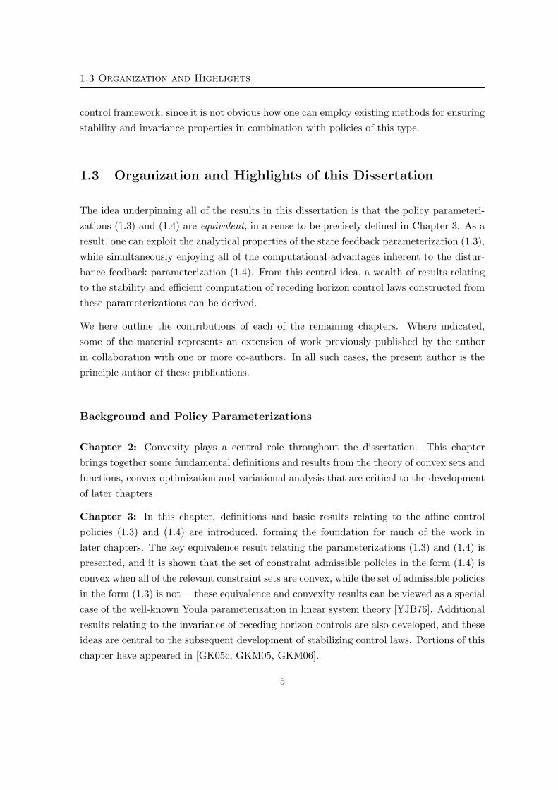
1.3 Organization and Highlights of this Dissertation
The idea underpinning all of the results in this dissertation is that the policy parameteri-
zations (1.3) and (1.4) are equivalent, in a sense to be precisely defined in Chapter 3. As a
result, one can exploit the analytical properties of the state feedback parameterization (1.3),
while simultaneously enjoying all of the computational advantages inherent to the distur-
bance feedback parameterization (1.4). From this central idea, a wealth of results relating
to the stability and efficient computation of receding horizon control laws constructed from
these parameterizations can be derived.
We here outline the contributions of each of the remaining chapters. Where indicated,
some of the material represents an extension of work previously published by the author
in collaboration with one or more co-authors. In all such cases, the present author is the
principle author of these publications.
Background and Policy Parameterizations
Chapter 2: Convexity plays a central role throughout the dissertation. This chapter
brings together some fundamental definitions and results from the theory of convex sets and
functions, convex optimization and variational analysis that are critical to the development
of later chapters.
Chapter 3: In this chapter, definitions and basic results relating to the affine control
policies (1.3) and (1.4) are introduced, forming the foundation for much of the work in
later chapters. The key equivalence result relating the parameterizations (1.3) and (1.4) is
presented, and it is shown that the set of constraint admissible policies in the form (1.4) is
convex when all of the relevant constraint sets are convex, while the set of admissible policies
in the form (1.3) is not — these equivalence and convexity results can be viewed as a special
case of the well-known Youla parameterization in linear system theory [YJB76]. Additional
results relating to the invariance of receding horizon controls are also developed, and these
ideas are central to the subsequent development of stabilizing control laws. Portions of this
chapter have appeared in [GK05c, GKM05, GKM06].
5

1. Introduction
Stability and Receding Horizon Control
Chapter 4: In this chapter, we consider the problem of finding a finite horizon control
policy in the form (1.3) that minimizes the expected value of a quadratic cost function.
It is shown that, using the equivalent parameterization (1.4), this problem can be posed
as a convex optimization problem. It is then shown how a receding horizon control law
synthesized from policies that are optimal in this sense can guarantee that the resulting
closed-loop system is input-to-state stable, and that the behavior of such a control law
matches that of a classical linear-quadratic or H2 control law when the system is operating
far from its constraints. General results relating to input-to-state stability of constrained
systems with convex Lyapunov functions are also developed in support of the main results.
This chapter is based largely on results appearing in [GK05b, GK06a].
Chapter 5: In this chapter, we employ an alternative quadratic cost function where the
disturbance is negatively weighted as inH∞ control [BB91, GL95], and consider the problem
of finding a control policy that minimizes the maximum value of this function. By imposing
additional convex constraints on the set of policies introduced in Chapter 3, we show that
this min-max optimization problem can be rendered convex-concave, making its solution
amenable in principle to standard techniques in convex optimization. We further show how
one can guarantee that if these policies are used in the synthesis of receding horizon control
laws, then the `2 gain of the resulting closed-loop system is bounded, and the achievable
bound decreases with the length of the planning horizon used by the controller. This chapter
expands on results appearing in [GKA06, GK06b].
Computational Methods
Chapter 6: In the theoretical results of Chapters 4 and 5, receding horizon control laws
are proposed that require the repeated solution of finite horizon control problems that are
solvable in principle using convex optimization techniques. In this chapter we consider the
problem of calculating such optimal policies in practice. It is argued that the problem of
finding such optimal policies is generally only feasible when the state and input constraints
are characterized by linear inequalities, though the disturbance set can be characterized in
a large variety of ways. Of particular interest in engineering applications are polytopic or
norm-bounded disturbance sets, and each of these is considered in turn for the problems
posed in Chapters 3–5. In all of the cases considered, the central result is that a feasible or
optimal affine state feedback policy can be found by solving a single convex optimization
6

1.3 Organization and Highlights
problem, in one of a variety of standard forms, whose size is polynomially bounded in the
size of the problem data.
Chapter 7: In this chapter, the solution to one of the convex optimization problems pre-
sented in Chapter 6 — the problem of finding a policy that minimizes a quadratic function
of the nominal state and input sequences of a system subject to ∞–norm bounded distur-
bances — is considered in significantly greater detail. In its original form, this optimization
problem is a dense convex quadratic program with O(N 2) variables, assuming that the
horizon length N dominates the number of states and control inputs at each stage. Hence
each iteration of an interior-point optimization method would require the solution of a dense
linear system in O(N6) operations.
We show how structure can be exploited to devise a sparse formulation of this problem,
thereby realizing a substantial reduction in computational effort to O(N 3) work per interior-
point iteration. This sparse formulation is the result of a decomposition technique that can
be used to separate the problem into a coupled set of finite horizon control problems.
The reduction of effort is the analogue, for robust control, to the situation in classical
unconstrained optimal control in which Linear Quadratic Regulator (LQR) problems can be
solved in O(N) time, using a Riccati [AM90, Sec. 2.4] or Differential Dynamic Programming
[JM70] technique in which the state feedback equation x+ = Ax + Bu is explicit in every
stage, compared to O(N 3) time for the more compact formulation in which states are
eliminated from the system. More direct motivation for these results comes from [Wri93,
Ste95, RWR98, Bie00, DBS05], which describe efficient implementations of optimization
methods for solving optimal control problems with state and control constraints, though
without disturbances. Much of the work in this chapter is based on [GK05a, GKR07].
Output Feedback Extensions and Conclusion
Chapter 8: All of the results of Chapters 3–7 relate to the application of the policy param-
eterization (1.3) and its associated reparameterization (1.4) to problems where a complete
measurement of the state is available. In this chapter, an analogous reparameterization for
output feedback control is employed in conjunction with a fixed linear state observer and a
corresponding bound on the state estimation error.
The main aim of the chapter is to provide conditions under which receding horizon control
laws synthesized from this parameterization can guarantee constraint satisfaction for all
time. When the state estimation error bound matches the minimal robust positively in-
7

1. Introduction
variant (mRPI) set for the system error dynamics, we show that the control law is actually
time-invariant, but its calculation requires the solution of an infinite-dimensional optimiza-
tion problem when the mRPI set is not finitely determined. By employing an invariant
outer approximation to the mRPI error set [RKKM05], we develop a time-invariant control
law that can be computed by solving a finite-dimensional tractable optimization problem at
each time step. The computational complexity of the proposed control law does not differ
greatly from the state feedback results of previous chapters, so the main technical difficulties
encountered with the output feedback problem considered here relate to the specification of
appropriate conditions on the initial error set and terminal state such that the closed-loop
system is robust positively invariant under a finitely determined time-invariant controller.
This work has also appeared in [GK07, GK06c].
Chapter 9: This chapter summarizes the main contributions of the dissertation and sug-
gests some directions for future research.
8

Chapter 2. Background
In this chapter we collect various definitions and useful results relating to convexity and
convex optimization. The selection of results presented is dictated entirely by their use in
subsequent chapters; for a thorough review of convex analysis and optimization, the reader
is referred to the excellent texts [Roc70, RW98, BNO03, BV04], from which many of the
results and definitions are drawn.
2.1 Convex Sets
Definition 2.1 (Convex Set). A set C ⊆ Rn is a convex set if, for every pair of points
x ∈ C and y ∈ C, every point on the line connecting them is also contained in C, i.e.
(1− τ)x + τy ∈ C, for all τ ∈ (0, 1). (2.1)
Convex sets play a central role in almost all of the results to be presented in this dissertation.
Although many of the theoretical results to be presented will be based on abstract convex
sets without any special structure, several specific classes of convex sets will also be used,
particularly when dealing with computational problems.
Example 2.2 (Polyhedra and Polytopes). A set is C ⊆ Rn is a polyhedron if it can
be defined by a set of affine inequalities
C := x ∈ Rn | Ax ≤ b (2.2)
for some matrix A ∈ Rt×n and vector b ∈ R
t, where t is the number of inequalities defining
the set. The set C is a polytope if it is a bounded polyhedron. Both polyhedra and polytopes
are convex sets.
9

2. Background
Convex Sets Nonconvex Sets
Figure 2.1: Examples of convex and nonconvex sets
Example 2.3 (Norm Balls). Given any norm ‖·‖ in Rn, the set
B := x ∈ Rn | ‖x‖ ≤ 1
is a convex set. The set is called a norm ball for the norm ‖·‖.
We will often use norm balls defined by the p–norms ‖·‖p, and so use the notation
Bnp := x ∈ R
n | ‖x‖p ≤ 1
for these sets. Some examples of convex and nonconvex sets are shown in Figure 2.1.
A particular class of convex set that we will encounter when dealing with certain optimiza-
tion problems is the convex cone:
Definition 2.4 (Convex Cones). A set K ⊆ Rn is a convex cone if it is convex and if,
for every pair of points x ∈ K and y ∈ K and scalars τ1 and τ2,
τ1x + τ2y ∈ C, for all (τ1, τ2) ≥ 0. (2.3)
A set K is called a proper cone if it is a closed convex cone with nonempty interior that
does not contain any line, i.e. the only x ∈ K also satisfying −x ∈ K is the origin.
Example 2.5 (Semidefinite Cone). The set of symmetric positive semidefinite matrices
in Rn×n
Q ∈ Rn×n | Q º 0
is called the semidefinite cone.
10

2.1 Convex Sets
Example 2.6 (Norm Cone). Given any norm ‖·‖ in Rn, the set
(
x
t
) ∣
∣
∣
∣
∣
‖x‖ ≤ t
⊆ Rn+1
is called the norm cone associated with the norm ‖·‖.
Both the semidefinite cone and the norm cones for every norm are proper cones.
2.1.1 Convex Hulls
If a set C is not convex, then it can be ‘convexified’ by taking its convex hull, i.e. the smallest
convex set containing C, denoted conv (C). An alternative (and equivalent) definition of the
convex hull of a set C is the set of all convex combinations of points in C, where a convex
combination of vectors x1, . . . , xn is any linear combination∑n
i=1 λixi with nonnegative
weights λi satisfying∑n
i=1 λi = 1.
A useful result for relating points in conv(C) to points in C is Caratheodory’s Theorem:
Theorem 2.7 (Caratheodory’s Theorem). If the set C ∈ Rn is nonempty, then every
point x ∈ conv(C) can be written as a convex combination of n + 1 points (not necessarily
different) in C.
2.1.2 Operations on Convex Sets
Of special interest will be those operations that, when applied to a closed and convex set
C, preserve convexity and closedness. We here outline a number of such operations that
are most relevant to subsequent results:
Proposition 2.8 (Set Intersections).
i. The intersection of an arbitrary collection of convex sets is convex.
ii. The intersection of an arbitrary collection of closed sets is closed.
iii. The intersection of a finite collection of polyhedral sets is polyhedral.
11

2. Background
PSfrag replacements
x
y
Figure 2.2: Loss of closedness under the linear mapping f(x, y) = x.
Proposition 2.9 (Set Addition).
i. C ⊕D is a convex set if C and D are convex.
ii. C ⊕ D is a closed set if C and D are closed and at least one of the sets is nonempty
and bounded.
iii. C ⊕ D is a closed set if C and D are orthogonal, i.e. if c ⊥ d for all c ∈ C and all
d ∈ D.
Proposition 2.10 (Linear Mappings). If L : Rn → R
m is a linear mapping and C ⊆ Rn
is a convex set, then
i. L(C) is a convex set.
ii. If C is also closed, then a sufficient condition for L(C) to be closed is that there does
not exist any nonzero y such that L(y) = 0 and such that x + λy ∈ C for all x ∈ C and
all λ ≥ 0.
iii. If C is polyhedral, then L(C) is polyhedral.
It is important to note that it is possible for a set to lose closedness under a linear mapping
if the conditions of Prop. 2.10(ii) do not hold, though these conditions are not necessary
ones. An example of such a situation is shown in Figure 2.2.
12
2.1 Convex Sets
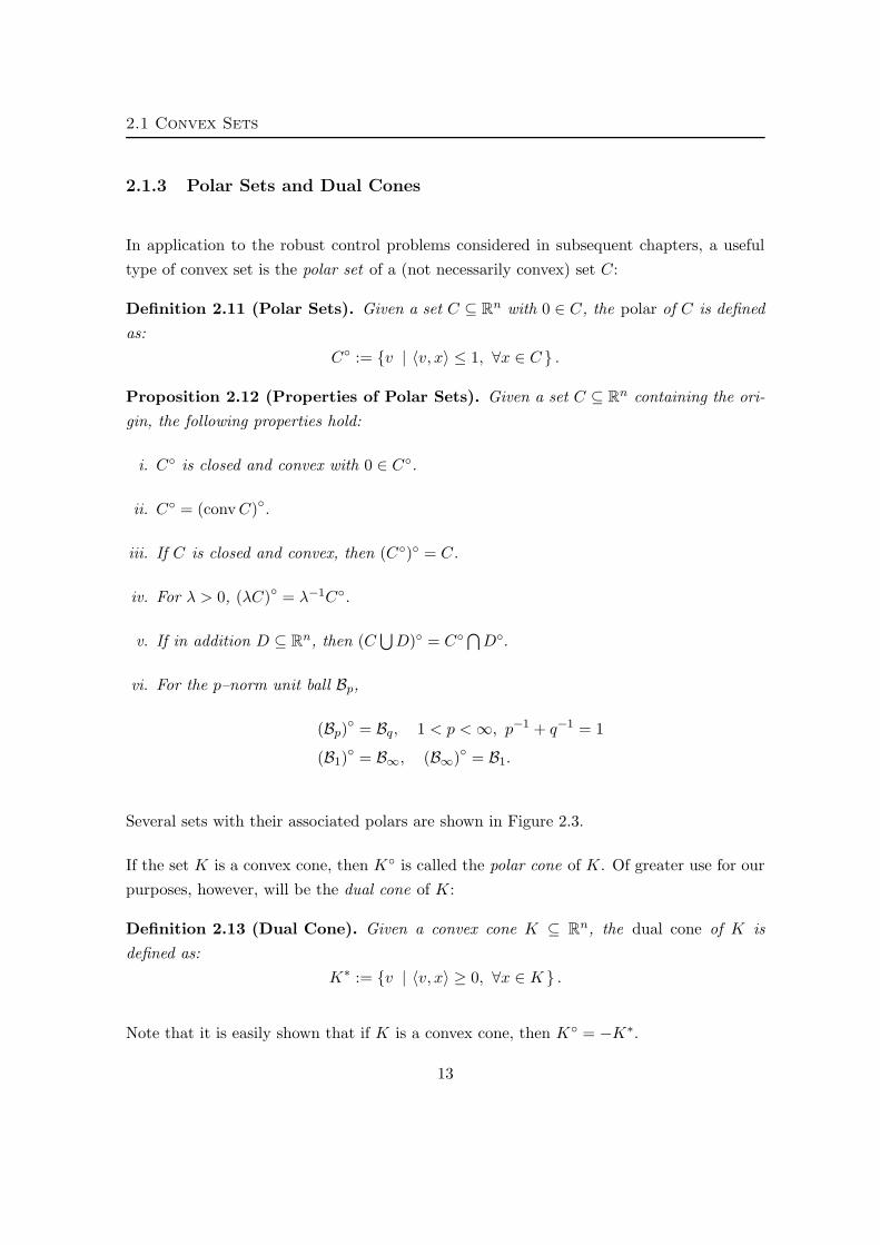
2.1.3 Polar Sets and Dual Cones
In application to the robust control problems considered in subsequent chapters, a useful
type of convex set is the polar set of a (not necessarily convex) set C:
Definition 2.11 (Polar Sets). Given a set C ⊆ Rn with 0 ∈ C, the polar of C is defined
as:
C := v | 〈v, x〉 ≤ 1, ∀x ∈ C .
Proposition 2.12 (Properties of Polar Sets). Given a set C ⊆ Rn containing the ori-
gin, the following properties hold:
i. C is closed and convex with 0 ∈ C.
ii. C = (conv C).
iii. If C is closed and convex, then (C) = C.
iv. For λ > 0, (λC) = λ−1C.
v. If in addition D ⊆ Rn, then (C
⋃
D) = C⋂
D.
vi. For the p–norm unit ball Bp,
(Bp) = Bq, 1 < p <∞, p−1 + q−1 = 1
(B1) = B∞, (B∞) = B1.
Several sets with their associated polars are shown in Figure 2.3.
If the set K is a convex cone, then K is called the polar cone of K. Of greater use for our
purposes, however, will be the dual cone of K:
Definition 2.13 (Dual Cone). Given a convex cone K ⊆ Rn, the dual cone of K is
defined as:
K∗ := v | 〈v, x〉 ≥ 0, ∀x ∈ K .
Note that it is easily shown that if K is a convex cone, then K = −K∗.
13

2. Background
−2 −1.5 −1 −0.5 0 0.5 1 1.5 2−2
−1.5
−1
−0.5
0
0.5
1
1.5
2
⇔
−2 −1.5 −1 −0.5 0 0.5 1 1.5 2−2
−1.5
−1
−0.5
0
0.5
1
1.5
2
−2 −1.5 −1 −0.5 0 0.5 1 1.5 2−2
−1.5
−1
−0.5
0
0.5
1
1.5
2
⇔
−2 −1.5 −1 −0.5 0 0.5 1 1.5 2−2
−1.5
−1
−0.5
0
0.5
1
1.5
2
−2 −1.5 −1 −0.5 0 0.5 1 1.5 2−2
−1.5
−1
−0.5
0
0.5
1
1.5
2
⇔
−2 −1.5 −1 −0.5 0 0.5 1 1.5 2−2
−1.5
−1
−0.5
0
0.5
1
1.5
2
−2 −1.5 −1 −0.5 0 0.5 1 1.5 2−2
−1.5
−1
−0.5
0
0.5
1
1.5
2
⇔
−2 −1.5 −1 −0.5 0 0.5 1 1.5 2−2
−1.5
−1
−0.5
0
0.5
1
1.5
2
−2 −1.5 −1 −0.5 0 0.5 1 1.5 2−2
−1.5
−1
−0.5
0
0.5
1
1.5
2
⇔
−2 −1.5 −1 −0.5 0 0.5 1 1.5 2−2
−1.5
−1
−0.5
0
0.5
1
1.5
2
Figure 2.3: Convex Sets and Polar Sets
14

2.2 Convex Functions
2.2 Convex Functions
Definition 2.14 (Convex Function). A function f : Rn → R is a convex function rela-
tive to the set C ⊆ Rn if, for every pair of points x ∈ C and y ∈ C, the following inequality
holds:
f ((1− τ)x + τy) ≤ (1− τ)f(x) + τf(y), for all τ ∈ (0, 1). (2.4)
The function f is strictly convex if the inequality (2.4) is strict.
A function f : Rn → R is called concave if −f is convex.
Note that the function f in Def. 2.14 assigns a value on the extended real line R (i.e. the set
R ∪ −∞,∞) to every value in Rn. The effective domain of f , denoted dom f , is defined
as
dom f := x | f(x) <∞ .
The function f is proper if f(x) <∞ for at least one x ∈ Rn (i.e. dom f is nonempty) and
the function never takes the value −∞. Note that if a convex function g : C → R is defined
only on a convex set C, then one can identify it with a convex function f satisfying the
conditions of Def. 2.14 by defining
f(x) :=
g(x) if x ∈ C
∞ if x /∈ C.
Proposition 2.15. A convex function is continuous on the interior of its effective domain.
Note, however, that a convex function is not guaranteed to be continuous at the boundary
of its domain. For example, the convex function in Figure 2.4 is discontinuous at the point
x, though it is upper semicontinuous everywhere.
2.2.1 Operations on Convex Functions
As in the case of convex sets, there are a number of operations which, when applied to
convex functions, preserve convexity and semicontinuity. The most relevant of these to the
work presented here are the following:
Proposition 2.16 (Addition and scaling). Given convex functions fi : Rn → R and
scalars λi ∈ R, the function∑
i∈I λifi is convex if each λi ≥ 0, and strictly convex if at
least one function fi is strictly convex with λi > 0.
15

2. Background
PSfrag replacementsx
Figure 2.4: A discontinuous convex function.
Proposition 2.17 (Pointwise supremum).
i. The pointwise supremum of an arbitrary collection of convex functions is convex.
ii. The pointwise supremum of an arbitrary collection of lower semicontinuous functions
is lower semicontinuous.
2.2.2 Support and Gauge Functions
Of particular interest in our development of robust control policies will be two convex
functions defined in relation to a convex set C. These are the support function and the
gauge function:
Definition 2.18 (Support and Gauge Functions). Given a convex set C ⊆ Rn, the
support function σC : Rn → R is defined as:
σC(x) := supy∈C
(x>y).
If 0 ∈ C, the gauge function γC : Rn → R is defined as:
γC(x) := inf λ ≥ 0 | x ∈ λC .
For a closed set C, the support and gauge functions have straightforward geometric inter-
pretations; the set
y∣
∣ x>y = σC(x)
defines a plane tangent to C with normal vector x,
while λ = γC(x) is the smallest amount by which C can be scaled while guaranteeing that
x ∈ λC (see Figure 2.5).
16

2.3 Convex Optimization
PSfrag replacements
x
C
λC
x>y = σC(x)
Figure 2.5: Support and Gauge Functions
The support and gauge functions of a set C have several properties that will be useful in
subsequent sections; principal among these properties is their relation to one another with
respect to the polar set C:
Proposition 2.19 (Properties of Support and Gauge Functions). If C is a closed
and convex set with 0 ∈ C, the following properties hold:
i. σC(·) ≥ 0.
ii. σC(·) = γC(·) and γC(·) = σC(·).
iii. If C is also compact and symmetric (i.e. x ∈ C implies (−x) ∈ C), then its gauge
function γC corresponds to a norm. In particular, for the p–norm ball Bp, γBp = ‖·‖pwhere 1 ≤ p ≤ ∞.
2.3 Convex Optimization
A convex optimization problem is a minimization problem in the form
minx
f0(x)
subject to:fi(x) ≤ 0, ∀i ∈ 1, . . . , pgi(x) = 0, ∀i ∈ 1, . . . , q,
(2.5)
17

2. Background
where each of the functions fi : Rn → R is a convex function, and each of the functions
gi : Rn → R is affine. The function f0 is referred to as the cost or objective function,
while the remaining functions fi and gi are referred to as the problem constraints. Note
that a variety of problems can be cast in the general framework of (2.5), e.g. the problem of
maximizing a concave function can be recast as a convex optimization problem via a change
of sign.
Occasionally it will be of interest to find a feasible point for the problem (2.5), i.e. one
satisfying the constraints, without regard to optimality. The problem of finding such a
point is easily written in the form (2.5) by defining an optimization problem with zero
objective function:
minx
0
subject to:fi(x) ≤ 0, ∀i ∈ 1, . . . , pgi(x) = 0, ∀i ∈ 1, . . . , q.
(2.6)
As a result, we will generally refer to the problem of finding a point that satisfies some set
of convex constraints as a convex optimization problem, with the understanding that such
a problem can be posed in the form (2.6).
In the remainder of this section we outline some of the most important classes of convex
optimization problems.
2.3.1 Linear and Quadratic Programs
A quadratic program or QP is a problem in the form
minx
c>0x + 12x>Qx
subject to:c>ix ≤ di, ∀i ∈ 1, . . . , pa>ix = bi, ∀i ∈ 1, . . . , q.
(2.7)
The problem (2.7) is a convex optimization problem if the matrix Q º 0, and we will
generally assume that this is the case. If Q = 0, then the objective function in (2.7) is
linear, and the problem is referred to as a linear program or LP.
Note that the problem of finding a point x ∈ C, where C is a polyhedral set defined as
in (2.2), is a feasibility problem which can be cast as an LP.
18

2.3 Convex Optimization
2.3.2 Second-Order Cone Programs
A second-order cone program or SOCP is a convex optimization problem in the form
minx
c>0x
subject to:‖Cix + di‖2 ≤ a>ix + bi, ∀i ∈ 1, . . . , p
a>ix = bi, ∀i ∈ 1, . . . , q.(2.8)
Note that if each of the matrices Ci and vectors di is zero, then (2.8) reduces to a linear
program. More generally, any convex quadratic program can be written as a second-order
cone program using appropriate variable transformations [LVBL98].
2.3.3 Linear Matrix Inequalities and Semidefinite Programs
A linear matrix inequality or LMI is a constraint in the form
F (x) := F0 +
n∑
i=1
Fixi ¹ 0, (2.9)
where each of the matrices Fi is symmetric and x := (x1, . . . , xn). An LMI constraint in
the form (2.9) is a convex constraint on x, i.e. x | F (x) ¹ 0 is a closed and convex set.
The same result holds if the LMI constraint in (2.9) is strict, i.e. F (x) ≺ 0, although in this
case the set x | F (x) ≺ 0 is open.
Note that inequalities involving matrix valued variables can be written in the standard
form (2.9). For example, the problem of finding a solution to the discrete-time Lyapunov
inequality
A>PA− P ≺ 0 (2.10)
can be written in the form (2.9) by defining an appropriate basis set P1, . . . Pm for the
symmetric matrix variable P ∈ Rn×n, where m = n(n + 1)/2, and defining F0 = 0 and
Fi := A>PiA − Pi. Matrix inequalities such as (2.10) are therefore generally referred to as
LMIs when it is clear from the context which matrices are intended as variables, with the
understanding that they can be converted to the form (2.9) when necessary.
The following Lemma often proves useful in rewriting some matrix inequalities in LMI form:
19

2. Background
Lemma 2.20 (Schur Complement). If A, B and C are real matrices of compatible di-
mension with
X :=
(
A B
B> C
)
,
then the following results hold:
i. X ≺ 0 if and only if C ≺ 0 and (A−BC−1B>) ≺ 0.
ii. If C ≺ 0, then X ¹ 0 if and only if A−BC−1B>¹ 0.
iii. X ¹ 0 if and only if C ¹ 0, (A−BC†B>) ¹ 0 and B(I − CC†) = 0.
iv. X is invertible if both C and (A−BC−1B>) are invertible.
A semidefinite program or SDP is a problem in the form
minx
c>x
subject to: F0 +n∑
i=1
Fixi ¹ 0.(2.11)
Note that multiple LMI constraints are easily handled via appropriate redefinition of the ma-
trices Fi. Both QPs and SOCPs can be considered subclasses of semidefinite programming
problems, since both problem types can be written in the general form (2.11). However, it
is generally better to solve a problem as an SOCP or QP if it is possible to do so, since
stronger computational complexity guarantees are generally possible for QPs and SOCPs
than for SDPs [LVBL98], and computational methods and software for these problems are
more mature.
2.3.4 Generalized Inequalities and Conic Programs
Given a proper cone K ⊆ Rn, we can define a generalized inequality as a partial ordering
on Rn using K:
a ¹K
b ⇔ b− a ∈ K (2.12a)
a ≺K
b ⇔ b− a ∈ int (K). (2.12b)
Analogous expressions are used to define the inequalities ºK
and ÂK. Note that the familiar
element-wise inequality ≤ on Rn is equivalent to (2.12) with K equal to the nonnegative
20

2.4 Parametric Minimization
orthant Rn+. The usual inequality for matrices A º B is also equivalent to (2.12) with K
equal to the positive semidefinite cone.
The simplest form of convex optimization problem involving generalized inequalities is one
with a single affine inequality:
minx
c>x
subject to:Cx ¹
Kd
Ax = b.
(2.13)
A problem in this form is called a cone program. The problem formulations for LPs, SOCPs
and SDPs can all be treated as special cases of cone programs.
2.4 Parametric Minimization
Given a convex function f : Rn × R
m → R, we will often want to minimize the function
f(x, u) with respect to the variable u only. Such a problem is referred to as a parametric
minimization problem. This section presents some of the characteristics of the function
minu f(x, u) with respect to x, as well as the properties of the minimizers of this function.
In the control applications to be presented in subsequent chapters, the variable x will
generally represent the state of a dynamic system, and the variables u will represent some
collection of parameters determining a control strategy for the system. Of particular interest
are conditions guaranteeing that the function infu f(x, u) is convex and lower semicontinuous
with respect to x, so that the resulting function can be employed as a Lyapunov function in
establishing results on stability. Additionally, we are interested in conditions ensuring that
the sets argminu f(x, u) are single-valued and continuous with respect to x, so that control
laws defined by these minimizers can be guaranteed to have these properties.
We first require some preliminary definitions and results:
Definition 2.21 (Uniform Level Boundedness [RW98, Defn. 1.16]). A function f :
Rn × R
m → R taking values f(x, u) is said to be level bounded in u locally uniformly in x
if, for each x ∈ Rn and α ∈ R, there exists a set V ⊆ R
n and a bounded set B ⊂ Rn such
that x ∈ int(V ) and
u | f(x, u) ≤ α ⊆ B, for all x ∈ V.
21

2. Background
The conditions of Def. 2.21 are more general than is strictly necessary for our purposes. We
will therefore employ the following result establishing sufficient conditions for a function to
meet these requirements.
Proposition 2.22. A function f : Rn × R
m → R taking values f(x, u) is level bounded in
u locally uniformly in x if there exists a function g : Rn × R
m → R defined as
g(x, u) := ‖Cx + Du‖c ,
such that g(x, u) ≤ f(x, u) for all x and u, where ‖·‖ is any norm, D is full column rank
and c > 0.
Proof. We first show that g(x, u) is level bounded in u locally uniformly in x. Choose
any x ∈ Rn and α ∈ R, and define V = x + δx | ‖δx‖ ≤ 1 so that x ∈ int(V ). From
Definition 2.21, it is sufficient to show that
⋃
x∈V
u | ‖Cx + Du‖c ≤ α ⊆ B
for some bounded set B. Restricting α and α1c to be positive without loss of generality,
⋃
x∈V
u | ‖Cx + Du‖c ≤ α =⋃
x∈V
u∣
∣
∣‖Cx + Du‖ ≤ α
1c
⊆⋃
x∈V
u∣
∣
∣ ‖Du‖ ≤ α1c + ‖Cx‖
⊆
u
∣
∣
∣
∣
∣
‖Du‖ ≤ α1c + ‖Cx‖+ sup
‖δx‖≤1‖Cδx‖
, (2.14)
where the latter two expressions come from straightforward application of the properties of
vector norms. The set in the right hand side of (2.14) is bounded since the matrix D is full
column rank [HJ85, Thm. 5.3.2 & Cor. 5.4.8], establishing the result for g(x, u). The result
follows for f(x, u) since the inequality g(x, u) ≤ f(x, u) guarantees
u | f(x, u) ≤ α ⊆ u | g(x, u) ≤ α
for all x ∈ V .
22

2.4 Parametric Minimization
Proposition 2.23 (Parametric Optimization). Let f : Rn × R
m → R be a convex,
proper and lower semicontinuous function and define
p(x) := infu
f(x, u), P (x) := argminu
f(x, u).
Properties of p
i. The function p is convex on Rn.
ii. The function p is also lower semicontinuous and proper on Rn if either;
(a) f(x, u) is level bounded in u locally uniformly in x, or
(b) for some x ∈ Rn the set P (x) is nonempty and bounded.
Properties of P
If f(x, u) is also level bounded in u locally uniformly in x then;
iii. For each x ∈ dom(p), the set P (x) is nonempty, convex and compact. If x /∈ dom(p),
then P (x) = ∅.
iv. If in addition f(x, u) is strictly convex in u, then P is single valued on dom(P ) and
continuous on int(dom(P )).
Proof. The proposition is a combination of various standard results in convex analysis.
Convexity of f is sufficient to establish convexity of the function p and of the set P (x) for
each x [RW98, Prop. 2.22] in (i) and (iii). The remainder of the results in (iii) rely on f
being lower semicontinuous and proper with f(x, u) level bounded in u locally uniformly in
x [RW98, Prop. 1.17]. The alternative results (iia) and (iib) come from [RW98, Prop. 1.17]
and [RW98, Cor. 3.32] respectively. Part (iv) is from [RW98, Thm. 3.31] and [RW98,
Cor. 7.43].
Some care is required when considering the continuity or convexity of functions that result
from convex parametric minimization – recall that not all convex functions are continuous
(cf. Figure 2.4). When minimizing a convex function over a subset of its variables, it is not
the case that continuity will be preserved, even if the original function is strictly continuous
on its effective domain. The following example illustrates this point:
23
2. Background
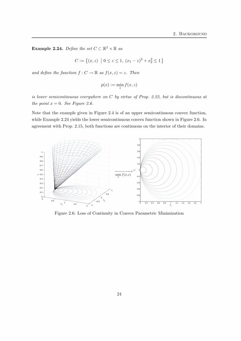
Example 2.24. Define the set C ⊂ R2 × R as
C :=
(x, z)∣
∣ 0 ≤ z ≤ 1, (x1 − z)2 + x22 ≤ 1
and define the function f : C → R as f(x, z) = z. Then
p(x) := minz
f(x, z)
is lower semicontinuous everywhere on C by virtue of Prop. 2.23, but is discontinuous at
the point x = 0. See Figure 2.6.
Note that the example given in Figure 2.4 is of an upper semicontinuous convex function,
while Example 2.24 yields the lower semicontinuous convex function shown in Figure 2.6. In
agreement with Prop. 2.15, both functions are continuous on the interior of their domains.
00.5
11.5
2 −1
−0.5
0
0.5
1
0
0.1
0.2
0.3
0.4
0.5
0.6
0.7
0.8
0.9
1
x2
x1
z
−−−−−−→min
zf(x,z)
x1
x 2
0 0.2 0.4 0.6 0.8 1 1.2 1.4 1.6 1.8 2−1
−0.8
−0.6
−0.4
−0.2
0
0.2
0.4
0.6
0.8
1
Figure 2.6: Loss of Continuity in Convex Parametric Minimization
24

Chapter 3. Affine Feedback Policies and Robust Control
3.1 Problem Definition
Consider the following discrete-time LTI system:
x+ = Ax + Bu + Gw, (3.1)
where x ∈ Rn is the system state at the current time instant, x+ is the state at the next
time instant, u ∈ Rm is the control input and w ∈ R
l is an external disturbance.
The current and future values of the disturbance are unknown and may change unpre-
dictably from one time instant to the next, but are assumed to be contained in a known
set W . The actual values of the state, input and disturbance at time instant k will be
denoted by x(k), u(k) and w(k), respectively.
Where it is clear from the context, x, u and w will be used to denote the current value of the
state, input and disturbance (note that since the system is time-invariant, the current time
can always be taken as zero). For the majority of this dissertation it will be assumed that,
at each sample instant, a measurement of the state x is available, though this assumption
will be relaxed in Chapter 8.
The system is subject to mixed constraints on the state and input, so that the system must
satisfy
(x, u) ∈ Z, (3.2)
where Z ⊂ Rn×R
m. The constraints defining the set Z may arise from either hard physical
constraints (e.g. actuator or other physical plant limitations) or from other design objectives
based on safety or performance considerations. In either case, a design goal is to guarantee
that the state and input of the closed-loop system remain in Z for all time and for all
disturbance sequences generated from the set W .
25

3. Affine Feedback Policies and Robust Control
Since the disturbance does not necessarily decay to zero, it may not be possible to drive the
state of the system to the origin. Instead, the best one can hope for is to drive the state of
the system to a target/terminal constraint set Xf ⊂ Rn. In this chapter, it will be shown
how, in conjunction with appropriately defined finite horizon control policies, the set Xf
can be used as a target set in time-optimal control or as a terminal constraint in a receding
horizon controller with guaranteed invariance properties.
We will make use of the following assumptions about this system throughout:
A3.1 (Standing Assumptions)
i. The pair (A, B) is stabilizable.
ii. The matrix G has full column rank.
iii. The state and input constraint set Z ⊆ Rn × R
m is closed, convex, contains the origin
in its interior and is bounded in the inputs, i.e. there exists a bounded set B such that
Z ⊆ Rn ×B.
iv. The terminal constraint set Xf ⊆ Rn is closed, convex and contains the origin in its
interior.
v. The disturbance set W is compact and contains the origin in its interior.
Note that the assumption that G is full column rank and that the origin is in the interior
of W are not unnecessarily restrictive; in cases where W contains the origin in its relative
interior1 and/or G is not full column rank, one may redefine W and G suitably such that
the stated assumptions hold.
3.1.1 Notation
In the sequel, predictions of the system’s evolution over a finite control/planning horizon
will be used to define a number of suitable control policies. Let the length N of this planning
horizon be a positive integer and define stacked versions of the predicted input, state and
1 The relative interior of a convex set C is the interior of C with respect to the smallest affine subsetcontaining C. See, for example, [Roc70, Sect. 5].
26

3.1 Problem Definition
disturbance vectors u ∈ RmN , x ∈ R
n(N+1) and w ∈ RlN , respectively, as
x :=
x0
x1
...
xN
, u :=
u0
u1
...
uN−1
, w :=
w0
w1
...
wN−1
(3.3)
where x0 =: x denotes the current measured value of the state and xi+1 := Axi+Bui+Gwi,
i = 0, . . . , N − 1 denotes the prediction of the state after i time instants.
Let the set W := W N := W × · · · ×W , so that w ∈ W, and define a closed and convex set
Z, appropriately constructed from Z and Xf , such that the constraints to be satisfied are
equivalent to (x,u) ∈ Z, i.e.
Z :=
(x,u)
∣
∣
∣
∣
∣
(xi, ui) ∈ Z, ∀i ∈ Z[0,N−1]
xN ∈ Xf
. (3.4)
Finally, define the matrices A ∈ Rn(N+1)×n and E ∈ R
n(N+1)×nN as
A :=
In
A
A2
...
AN
, E :=
0 0 · · · 0
In 0 · · · 0
A In · · · 0...
.... . .
...
AN−1 AN−2 · · · In
,
and the matrices B ∈ RnN×mN , G ∈ R
nN×lN , B ∈ Rn(N+1)×mN and G ∈ R
n(N+1)×lN as
B := IN ⊗B, G := IN ⊗G, B := EB, G := EG,
respectively. Using these definitions in conjunction with the system dynamics (3.1), the
state sequence x can then be written in vectorized form as
x = Ax + EBu + EGw= Ax + Bu + Gw.
27

3. Affine Feedback Policies and Robust Control
3.2 A State Feedback Policy Parameterization
Finding an arbitrary finite horizon control policy that satisfies the constraints Z for all ad-
missible disturbance sequences generated from W is extremely difficult in general. Current
proposals for defining such policies generally require solution via robust dynamic program-
ming [MRVK06] or very large scale optimization problems [SM98]. As a result, we will find
it convenient to restrict the class of control policies considered to those that are affine in
the sequence of states, i.e. those in the form2
ui = gi +i∑
j=0
Ki,jxj , ∀i ∈ Z[0,N−1], (3.5)
where each Ki,j ∈ Rm×n and gi ∈ R
m. For notational convenience, we also define the block
lower triangular matrix K ∈ RmN×n(N+1) and stacked vector g ∈ R
mN as
K :=
K0,0 0 · · · 0...
. . .. . .
...
KN−1,0 · · · KN−1,N−1 0
, g :=
g0
...
gN−1,
, (3.6)
so that the input sequence (3.5) can be written in vectorized form as
u = Kx + g. (3.7)
For a given initial state x, we say that the pair (K,g) is admissible if the control policy (3.5)
guarantees that for all allowable disturbance sequences of length N , the constraints Z are
satisfied over the horizon i = 0, . . . , N − 1, and that the state is in the target set Xf at the
end of the horizon. More precisely, the set of admissible (K,g) is defined as
ΠsfN (x) :=
(K,g)
∣
∣
∣
∣
∣
∣
∣
∣
∣
∣
∣
∣
∣
∣
∣
(K,g) satisfies (3.6), x0 = x
xi+1 = Axi + Bui + Gwi
ui = gi +∑i
j=0Ki,jxj
(xi, ui) ∈ Z, xN ∈ Xf
∀i ∈ Z[0,N−1], ∀w ∈ W
, (3.8)
2 Since the current state x will be assumed known, it is possible to set K0,0 = 0 without loss of generality.However, presentation of the results in this chapter is somewhat simplified if we do not impose this constraint.
28
3.2 A State Feedback Policy Parameterization
or, in more compact form, as
ΠsfN (x) :=
(K,g)
∣
∣
∣
∣
∣
∣
∣
∣
∣
∣
∣
(K,g) satisfies (3.6)
x = Ax + Bu + Gw
u = Kx + g
(x,u) ∈ Z, ∀w ∈ W
. (3.9)
The set of initial states x for which an admissible control policy of the form (3.5) exists is
defined as
XsfN :=
x ∈ Rn∣
∣
∣Πsf
N (x) 6= ∅
. (3.10)
It is critical to note that it may not be possible to select a single policy pair (K,g) ∈ ΠsfN (x)
such that it is admissible for all x ∈ XsfN . Indeed, it is possible to find examples where there
exists a pair (x, x) ∈ XsfN × Xsf
N such that ΠsfN (x)
⋂
ΠsfN (x) = ∅. For problems of non-
trivial size, it is therefore necessary to calculate an admissible pair (K,g) on-line, given a
measurement of the current state x.
Once an admissible control policy is computed for the current state, there are many ways
in which it can be applied to the system; time-varying, time-optimal and receding horizon
implementations are the most common, and are considered in detail in Section 3.6.
It is important to emphasize that, due to the dependence of (3.9) on the current state x,
the implemented control policy will, in general, be a nonlinear function of the state x, even
though it may have been defined in terms of the class of affine state feedback policies of the
form (3.5).
Remark 3.1. Note that the state feedback policy (3.5) subsumes the well-known class of
“pre-stabilizing” control policies [Bem98, LK99, CRZ01], in which the control policy takes
the form ui = ci + Kxi, where K is fixed. In such schemes, the on-line computation is
limited to finding an admissible perturbation sequence ciN−1i=0 . It can also be shown to
subsume ’tube’-based schemes such as [MSR05] based on linear feedback.
3.2.1 Nonconvexity in Affine State Feedback Policies
Finding an admissible policy pair (K,g) ∈ ΠsfN (x), given the current state x, has been
believed to be a very difficult problem. This is due to the nonlinear relationship between x
and u in (3.9), which results in the following property:
29
3. Affine Feedback Policies and Robust Control
Proposition 3.2 (Nonconvexity). For a given state x ∈ XsfN , the set of admissible affine
state feedback control policies ΠsfN (x) is nonconvex, in general.
The truth of this statement is easily verified by considering the following example:
Example 3.3 (Nonconvexity in affine state feedback policies). Consider the SISO
system x+ = x + u + w with initial state x0 = 0, input constraint |u| ≤ 3, bounded distur-
bances |w| ≤ 1 and a planning horizon of N = 3. Consider a control policy of the form (3.5)
with g = 0 and K2,1 = 0, so that u0 = 0 and
u1 = K1,1w0 (3.11)
u2 = [K2,2(1 + K1,1)] w0 + K2,2w1 (3.12)
In order to satisfy the input constraints for all allowable disturbance sequences, the controls
ui must satisfy
|ui| ≤ 3, i = 1, 2, ∀w ∈ W (3.13)
or, equivalently,
maxw∈W
|ui| ≤ 3, i = 1, 2. (3.14)
Since the constraints on the components of w are independent, the input constraints are
satisfied for all w ∈ W if and only if
|K1,1| ≤ 3 (3.15)
|K2,2(1 + K1,1)|+ |K2,2| ≤ 3. (3.16)
It is straightforward to verify that the set of gains (K1,1, K2,2) which satisfy these constraints
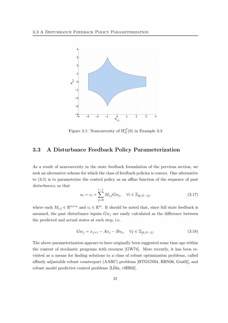
is nonconvex; the pairs (−3, 1) and (−1, 3) are acceptable, while the pair (−2, 2) is not. The
set of admissible values for (K1,1, K2,2), representing the intersection of the set ΠsfN (0) with
the plane g = 0, K1,2 = 0, is shown in Figure 3.1.
It is surprising to note that, though the set ΠsfN (x) may be nonconvex, the set Xsf
N is always
convex. Proof of this is deferred until Section 3.5. Additionally, despite the fact that ΠsfN (x)
may be nonconvex, we will show that one can still find an admissible (K,g) ∈ ΠsfN (x) by
solving an equivalent convex optimization problem.
30
3.3 A Disturbance Feedback Policy Parameterization
−4 −3 −2 −1 0 1 2 3 4−4
−3
−2
−1
0
1
2
3
4
K1,1
K2,
2
PSfrag replacements
K1,1
K2,2
Figure 3.1: Nonconvexity of ΠsfN (0) in Example 3.3
3.3 A Disturbance Feedback Policy Parameterization
As a result of nonconvexity in the state feedback formulation of the previous section, we
seek an alternative scheme for which the class of feedback policies is convex. One alternative
to (3.5) is to parameterize the control policy as an affine function of the sequence of past
disturbances, so that
ui = vi +i−1∑
j=0
Mi,jGwj , ∀i ∈ Z[0,N−1], (3.17)
where each Mi,j ∈ Rm×n and vi ∈ R
m. It should be noted that, since full state feedback is
assumed, the past disturbance inputs Gwj are easily calculated as the difference between
the predicted and actual states at each step, i.e.
Gwj = xj+1 −Axj −Buj , ∀j ∈ Z[0,N−1]. (3.18)
The above parameterization appears to have originally been suggested some time ago within
the context of stochastic programs with recourse [GW74]. More recently, it has been re-
visited as a means for finding solutions to a class of robust optimization problems, called
affinely adjustable robust counterpart (AARC) problems [BTGGN04, BBN06, Gus02], and
robust model predictive control problems [L03a, vHB02].
31

3. Affine Feedback Policies and Robust Control
For notational convenience, define the vector v ∈ RmN and the strictly block lower trian-
gular matrix M ∈ RmN×nN such that
M :=
0 · · · · · · 0
M1,0 0 · · · 0...
. . .. . .
...
MN−1,0 · · · MN−1,N−2 0
, v :=
v0
...
...
vN−1
, (3.19)
so that the input sequence (3.17) can be written in vectorized form as
u = MGw + v. (3.20)
In a manner similar to (3.8), define the set of admissible (M,v) as
ΠdfN (x) :=
(M,v)
∣
∣
∣
∣
∣
∣
∣
∣
∣
∣
∣
∣
∣
∣
∣
(M,v) satisfies (3.19), x0 = x
xi+1 = Axi + Bui + Gwi
ui = vi +∑i−1
j=0Mi,jGwj
(xi, ui) ∈ Z, xN ∈ Xf
∀i ∈ Z[0,N−1], ∀w ∈ W
(3.21)
or, in more compact form, as
ΠdfN (x) :=
(M,v)
∣
∣
∣
∣
∣
∣
∣
∣
∣
∣
∣
(M,v) satisfies (3.19)
x = Ax + Bu + Gw
u = MGw + v
(x,u) ∈ Z, ∀w ∈ W
. (3.22)
Define the set of initial states x for which an admissible control policy of the form (3.17)
exists as
XdfN :=
x ∈ Rn∣
∣
∣Πdf
N (x) 6= ∅
. (3.23)
Note that the state and disturbance feedback parameterizations (3.5) and (3.17) are qual-
itatively similar; in Section 3.5 we will show that they are actually equivalent. However,
the two parameterizations have slightly different interpretations, and we will require both
in order to establish various geometric and system-theoretic properties of receding horizon
control laws based on these policies.
32

3.4 Convexity and Closedness
In the next section, we discuss the main benefit of adopting the parameterization (3.17);
namely, that an admissible affine disturbance feedback policy can be found by solving a
convex and tractable optimization problem.
3.4 Convexity and Closedness
In this section we establish convexity and closedness of the sets ΠdfN (x) and Xdf
N . These prop-
erties will make the disturbance feedback parameterization (3.17) an attractive alternative
to the state feedback parameterization (3.5). Define the set
CN :=⋂
w∈W
(x,M,v)
∣
∣
∣
∣
∣
∣
∣
∣
∣
∣
∣
(M,v) satisfies (3.19)
x = Ax + Bu + Gw
u = MGw + v
(x,u) ∈ Z
. (3.24)
This set is closed and convex since it is the intersection of closed and convex sets. The set XdfN
can then be defined as a linear mapping of this set. However, the set CN is not guaranteed
to be compact when G is not full row rank or when the state and input constraints Z are
not bounded in the state dimension, so care must be taken to ensure that closedness is
preserved3 when treating XdfN as a linear mapping of CN .
Lemma 3.4. Given a linear mapping L : CN → Rs, if L(x,M,v) 6= 0 for every x 6= 0,
then the set L(CN ) is closed and convex.
Proof. A linear map of a convex set is always convex (Prop. 2.10). To ensure closedness,
define the set M and its orthogonal complement M⊥ as
M := M | M satisfies (3.19), My = 0, ∀y ⊥ R(G) (3.25a)
M⊥ := M | M satisfies (3.19), My = 0, ∀y ∈ R(G) . (3.25b)
Both of these sets are subspaces, with M∪M⊥ equal to the set of all matrices satisfy-
ing (3.19). Define the set
CN := CN ∩ (Rn ×M× RmN ), (3.26)
3Recall that, in general, a linear mapping of a closed but unbounded set is not guaranteed to be closed.See Figure 2.2.
33

3. Affine Feedback Policies and Robust Control
such that CN and CN differ only according to their inclusion of the subspace M⊥. Since
M⊥ is defined such that the nullspace of every element of M⊥ contains the set GW, it
follows that CN in (3.24) can alternatively be written as
CN = CN ⊕ (0 ×M⊥ × 0). (3.27)
Recalling that the state and input constraints Z are assumed bounded in the inputs and
the disturbance set W is assumed to contain the origin in its interior in A3.1, the setM is
also bounded, since maxw∈W ‖MGw‖ > 0 for any nonzero M ∈M. The set CN is therefore
bounded in policies, i.e. there exist bounded sets B1 ⊆ RmN×nN and B2 ⊆ R
mN such that
CN ⊆ (Rn ×B1 ×B2). Then
L(CN ) = L(
CN ⊕ (0 ×M⊥ × 0))
(3.28)
= L(
CN)
⊕ L
(
0 ×M⊥ × 0)
, (3.29)
where the latter relation follows since linear mappings are distributive with respect to
set addition. The set L(CN ) is closed since CN is compact in policies (Prop. 2.10(ii)), so
that (3.29) is the sum of closed and orthogonal sets, therefore also closed (Prop. 2.9).
We can now state the main result of this section:
Theorem 3.5 (Convexity). For every state x ∈ XdfN , the set of admissible affine distur-
bance feedback policies ΠdfN (x) is closed and convex. Furthermore, the set of states Xdf
N , for
which at least one admissible affine disturbance feedback policy exists, is also closed and
convex.
Proof. The set ΠdfN (x) represents a planar ‘slice’ through CN , and can be written as
ΠdfN (x) :=
⋂
w∈W
(M,v)
∣
∣
∣
∣
∣
∣
∣
∣
∣
∣
∣
(M,v) satisfies (3.19)
x = Ax + Bu + Gw
u = MGw + v
(x,u) ∈ Z
.
Like the set CN , the set ΠdfN (x) is closed and convex since it is the intersection of closed
and convex sets. The projection CN 7→ XdfN is a linear mapping satisfying the conditions of
Lem. 3.4, so XdfN is also closed and convex.
34

3.4 Convexity and Closedness
Remark 3.6. Convexity and closedness of the set CN will be important considerations when
establishing the properties of optimal finite horizon control policies in Chapters 4 and 5.
There we will need to minimize a convex and continuous objective function (x,M,v) 7→JN (x,M,v) over an effective domain restricted to CN . If CN is closed, then this function
is lower semicontinuous and the results of Section 2.4 will apply.
3.4.1 Handling Nonconvex Disturbance Sets
Recall that in A3.1, the set W was assumed to be convex and compact, with 0 ∈ int W .
We show here that if W (equivalently W) is nonconvex, it can be replaced with its convex
hull without loss of generality.
Proposition 3.7 (Convexification of W). The sets ΠdfN (x) and Xdf
N , defined in (3.21)
and (3.23) respectively, are unchanged if W is replaced with its convex hull.
Proof. For a given state x, define ΠdfN (x) to be the set of policies guaranteeing constraint
satisfaction for all W ∈ convW, i.e.
ΠdfN (x) :=
⋂
w∈convW
(M,v)
∣
∣
∣
∣
∣
∣
∣
∣
∣
∣
∣
(M,v) satisfies (3.19)
x = Ax + Bu + Gw
u = MGw + v
(x,u) ∈ Z
Since W ⊂ convW, ΠdfN (x) ⊂ Πdf
N (x) follows trivially. We show here that ΠdfN (x) ⊃ Πdf
N (x)
as well, so that ΠdfN (x) = Πdf
N (x).
From Caratheodory’s Theorem (Thm. 2.7), every element w ∈ convW ⊆ RlN can be
written as a convex combination of (lN + 1) points (not necessarily all different) in W.
Denote these points wi, so that w =∑(lN+1)
i=1 λiwi, where each λi ≥ 0 and∑(lN+1)
i=1 λi = 1.
Consider any control policy pair (M,v) ∈ ΠdfN (x), and define (x, u) :=
∑(lN+1)i=1 λi(xi,ui),
where
xi := Ax + Bv + (BMG + G)wi
ui := MGwi + v.
From the definition of ΠdfN (x), every pair (xi,ui) ∈ Z. Since the set Z is convex and
(x, u) is a convex combination of the points (xi,ui), it follows that (x, u) ∈ Z, so that
35

3. Affine Feedback Policies and Robust Control
(M,v) is constraint admissible for every w ∈ convW, i.e. (M,v) ∈ ΠdfN (x), and therefore
ΠdfN (x) ⊃ Πdf
N (x). This proves the result for the set ΠdfN (x); the result then follows for the
set XdfN directly from the definition (3.23).
Note that the above result is not indicative of excessive conservatism of the control policy
parameterization (3.17), since an equivalent result holds for control policies constructed via
robust dynamic programming techniques [BR71].
A consequence of Proposition 3.7 is that a wide variety of disturbance sets W can be handled
easily within the proposed framework, including nonconvex or disjoint sets, so long as W is
compact and 0 ∈ int (conv W ). We will therefore generally assume that W is a convex set
satisfying A3.1, with the understanding that we can replace W with conv W as necessary.
Corollary 3.8 (Polyhedral Sets). If the constraint sets Z and Xf are polyhedral and
the disturbance set W is a polytope, then the sets CN and XdfN are polyhedral and Πdf
N (x) is
polyhedral for each x ∈ XdfN .
Proof. If the set W (equivalently W) is a polytope, then the set of extreme disturbance se-
quences (i.e. those whose elements take values from the vertices ofW) is finite. Denote each
such extreme sequence wi, where i ∈ Z[1,q] for some finite integer q, so thatW≡conv wiqi=1.
The set CN can be written as
CN =⋂
wiqi=1
(x,M,v)
∣
∣
∣
∣
∣
∣
∣
∣
∣
∣
(M,v) satisfies (3.19)
x = Ax + Bu + Gwi
u = MGwi + v
(x,u) ∈ Z
, (3.30)
which is the intersection of a finite collection of polyhedral sets, and is thus also polyhedral
(Prop. 2.8). An identical argument establishes that ΠdfN (x) is polyhedral for each x ∈ Xdf
N .
The set XdfN is polyhedral since, as in the proof of Thm. 3.5, it can be written as a linear
mapping of CN , and any linear map of a polyhedral set is polyhedral (Prop. 2.10).
The results of this section will be of fundamental importance throughout this dissertation. If
W is convex and compact, then it is conceptually possible to compute a pair (M,v) ∈ ΠdfN (x)
in a computationally tractable way, given the current state x. Methods for calculating
policies in this class for particular characterizations of the sets Z and W will be addressed
in Chapter 6.
36
3.5 Equivalence of Affine Policy Parameterizations
3.5 Equivalence of Affine Policy Parameterizations
An important question is whether the disturbance feedback parameterization (3.17) is more
or less conservative than the state feedback parameterization (3.5). In this section, we show
that they are equivalent.
Theorem 3.9 (Equivalence). The set of admissible states XdfN = Xsf
N . Additionally,
given any x ∈ XsfN , for any admissible (K,g) an admissible (M,v) can be found which
yields the same state and input sequence for all allowable disturbance sequences, and vice-
versa.
Proof. The set equality is established by showing that both XsfN ⊆ Xdf
N and XdfN ⊆ Xsf
N .
XsfN ⊆ Xdf
N : By definition, for a given x ∈ XsfN , there exists a pair (K,g) ∈ Πsf
N (x) that
satisfies the constraints Z for all disturbance sequences w ∈ W. For a given w ∈ W, the
inputs and states of the system can be written as :
u = Kx + g (3.31)
= K(Ax + Bu + EGw) + g (3.32)
The matrix (I − KB) is always non-singular, since KB is strictly lower triangular. The
control sequence can then be rewritten as an affine function of the disturbance sequence w:
u = (I −KB)−1(KAx + g) + (I −KB)−1KEGw, (3.33)
and an admissible (M,v) constructed by choosing
M = (I −KB)−1KE (3.34a)
v = (I −KB)−1(KAx + g). (3.34b)
This choice of (M,v) gives exactly the same input sequence as the pair (K,g), so the state
and input constraints Z are satisfied for all disturbance sequences w ∈ W. The constraint
(3.19) that M be strictly block lower triangular is satisfied because M is chosen in (3.34) as
a product of the block lower triangular matrices (I −KB)−1 and K and the strictly block
lower triangular matrix E. Therefore, (M,v) ∈ ΠdfN (x) and thus x ∈ Xsf
N ⇒ x ∈ XdfN .
XdfN ⊆ Xsf
N : By definition, for a given x ∈ XdfN , there exists a pair (M,v) ∈ Πdf
N (x) that
satisfies the constraints Z for all disturbance sequences w ∈ W. For a given w ∈ W, the
37
3. Affine Feedback Policies and Robust Control
inputs and states of the system can be written as :
u = MGw + v (3.35)
x = Ax + B(MGw + v) + Gw (3.36)
Recalling that since full state feedback is assumed, one can recover the uncertain terms Gwi
using the relation
Gwi = xi+1 −Axi −Bui, ∀i ∈ Z[0,N−1], (3.37)
which can be written in matrix form as
Gw =
0 I 0 · · · 0
0 −A I. . .
......
. . .. . .
. . . 0
0 · · · 0 −A I
x−
I
0...
0
Ax− Bu, (3.38)
or more compactly as
Gw = E†x− IAx− Bu. (3.39)
It is easy to verify that the matrices E† and I> are left inverses of E and A respectively, so
that E†E = I and I>A = I. The input sequence can then be rewritten as
u = M(E†x− IAx− Bu) + v (3.40)
= (I + MB)−1(ME†x−MIAx + v). (3.41)
The matrix (I + MB) is non-singular because the product MB is strictly lower triangular.
An admissible (K,g) can then be constructed by choosing
K = (I + MB)−1ME† (3.42a)
g = (I + MB)−1(v −MIAx). (3.42b)
This choice of (K,g) gives exactly the same input sequence as the pair (M,v), so the
state and input constraints Z are satisfied for all disturbance sequences w ∈ W. The
constraint (3.6) that K be block lower triangular is satisfied because K is chosen in (3.42)
as a product of block lower triangular matrices. Therefore, (K,g) ∈ ΠsfN (x) and thus
x ∈ XdfN ⇒ x ∈ Xsf
N .
38

3.5 Equivalence of Affine Policy Parameterizations
Note that the proof of Theorem 3.9 is not predicated on any of the conditions of A3.1.
It is instead a direct consequence of the linearity of the system (3.1) and of the state and
disturbance feedback policies (3.5) and (3.17).
Recalling Theorem 3.5 leads next to the following result, which is surprising in light of the
potential nonconvexity of the set ΠsfN (x):
Corollary 3.10 (Convexity of XsfN ). The set of states Xsf
N , for which an admissible
affine state feedback policy of the form (3.5) exists, is a closed and convex set.
Remark 3.11. The results of Theorem 3.9 have appeared independently in [GKM06] and
[BBN06], with the latter appearing in the more general context of output feedback. In Chap-
ter 8, we present a generalization of the results in [BBN06] that incorporates nonzero initial
state estimates and observer dynamics, and provide several geometric and invariance results
paralleling those developed in this chapter.
An important consequence of Theorem 3.9 is that it provides a tractable method for finding
an affine state feedback policy (K,g) ∈ ΠsfN (x), a problem which has generally been con-
sidered intractable due to nonconvexity of the feasible set ΠsfN (x) (cf. Example 3.3). Since
the set ΠdfN (x) is convex, it is possible in principle to find a policy (M,v) ∈ Πdf
N (x) using
convex optimization methods; one can then find a policy (K,g) ∈ ΠsfN (x) via the transfor-
mation (3.42). Methods for calculating such policies for specific classes of disturbances and
constraint sets are discussed in Chapter 6.
Theorem 3.9 will also play a central role in the development of Chapters 4 and 5, where
we consider various system theoretic properties of receding horizon control laws derived
from the parameterizations (3.5) (equivalently, (3.17)). For many of the results, proof will
be significantly more straightforward using one or the other of the two parameterizations;
Theorem 3.5 will allow us to move freely between them, choosing whichever parameteriza-
tion is most natural or convenient in each context.
3.5.1 Relation to Pre-Stabilizing Control Policies
As a direct consequence of the equivalence result in Theorem 3.9, the class of affine feed-
back policies in the form ui = vi +∑i−1
j=0 Mi,jGwj subsumes the class of policies based on
perturbations to a fixed and pre-stabilizing linear control law in the form ui = ci + Kxi
(cf. Remark 3.1). We therefore conclude that, if the region of attraction for the class of
pre-stabilizing policies with fixed gain K is denoted XKN , then XK
N ⊆ XdfN always.
39

3. Affine Feedback Policies and Robust Control
However, we note that calculating a feasible policy pair (M,v) ∈ ΠdfN (x) for a given horizon
length N may require considerable computational effort; the number of decision variables
in the parameter M increase quadratically with the horizon length N , while the number of
decision variables ci in a pre-stabilizing scheme increases only linearly with N . A sensible
strategy might therefore be to employ a pre-stabilizing scheme with a longer horizon, in the
hope that XKN⊃ Xdf
N for some N > N , while still requiring less computational effort.
We next show that this is not always possible, and provide an example for which XKN
is a
strict subset of XdfN for some fixed N , regardless of how large we allow N to be:
Example 3.12. Consider the system
x+ = 2x + 2u + w,
subject to the following input and terminal constraints:
u ∈ u | |u| ≤ 0.7Xf = x | |x| ≤ 0.5
and subject to bounded disturbances |w| ≤ 0.25. We define a stabilizing controller K = −1.25.
For increasing horizon length N , we consider the size of the set XdfN for this system, as well
as the size of the set of feasible initial conditions XKN when the control policy for the system
is restricted to perturbations to the fixed linear feedback law u = Kx, i.e. those parameter-
ized as ui = ci + Kxi. The sizes of these sets with increasing horizon length are shown in
Figure 3.2, where it is clear that XKN⊂ Xdf
4for every N ∈ N.
Note that in Example 3.12 the terminal set Xf is robust positively invariant for the closed-
loop system x+ = (A + BK)x + w. Terminal conditions of this type will play a central role
in the development of robust receding horizon controls to be introduced in Section 3.6.
3.5.2 Relation to the Youla Parameter
The equivalence result of Thm. 3.9 is closely related to the well-known Youla parameteri-
zation from linear systems theory [YJB76][ZDG96, Ch. 12], where the problem of finding
a stabilizing linear controller for an unconstrained linear system is convexified via a similar
variable transformation. A useful method of comparison is to draw the sequence of inputs
resulting from the application of a given control policy (M,v) in block diagram form as
40

3.5 Equivalence of Affine Policy Parameterizations
0 5 10 150.5
0.6
0.7
0.8
0.9
1
1.1
1.2
1.3
Horizon Length N
Siz
e of
Fea
sibl
e S
et
PSfrag replacements
XdfN
XKN
Figure 3.2: Sizes of XdfN and XK
N with increasing N
in Figure 3.3 – such a figure has a structure usually employed in internal model control
(IMC) formulations for linear systems [GM82][Mac89, Ch.6] with stable plants, with the
feedback parameter M taking the place of the Youla parameter (typically denoted Q). Note
that it is not necessary to generalize this figure to the case of unstable plants, since the
policy (M,v) is only defined over a finite horizon.
It should be emphasized, however, that the feedback scheme shown in Figure 3.3 is strictly
notional – it will generally not be our intent to implement a calculated control policy
(M,v) in this manner. Instead, we will usually calculate and implement policies (M,v)
in a receding horizon fashion, resulting in static and nonlinear feedback control laws. In
this case Figure 3.3 represents an internal model employed by the controller in considering
possible future state trajectories resulting from a candidate control policy (M,v), and does
not represent the actual closed-loop behavior of the system. In the next section, we consider
the geometric and invariance properties of such receding horizon control laws.
41

3. Affine Feedback Policies and Robust Control
+++
+
−
+PSfrag replacementsv x
w
G
M
[
A B
I 0
]
[
A B
I 0
]
Figure 3.3: Internal Model Control
3.6 Geometric and Invariance Properties
It is well-known that the set of states for which an admissible open-loop input sequence exists
(i.e. one with K = 0 or M = 0) may collapse to the empty set if the horizon is sufficiently
large [SM98, Sect. F]. Furthermore, for time-varying, time-optimal or receding horizon
control implementations of the affine control policies defined in this chapter, it may not be
possible to guarantee constraint satisfaction for all time unless additional assumptions are
made. In this section, we provide conditions under which these problems will not occur. The
stability of receding horizon schemes based on these policies will be addressed in Chapters 4
and 5.
We first introduce the following standard assumption (cf. [MRRS00]):
A3.2 (Invariant Terminal Constraint) A state feedback gain matrix Kf and termi-
nal constraint set Xf have been chosen such that:
i. The matrix A + BKf is Hurwitz.
ii. Xf is contained inside the set of states for which the constraints (x, u) ∈ Z are satisfied
under the control u = Kfx, i.e. Xf ⊆ x | (x, Kfx) ∈ Z .
iii. Xf is robust positively invariant for the closed-loop system x+ = (A + BKf )x + Gw,
i.e. (A + BKf )x + Gw ∈ Xf for all x ∈ Xf and all w ∈W .
42

3.6 Geometric and Invariance Properties
Under some additional, mild technical assumptions, one can compute a Kf and a poly-
topic Xf that satisfies A3.2 when Z is a polytope and W is a polytope, an ellipsoid or
the affine map of a p-norm ball. The reader is referred to [Bla99, KG98, LK99] and the
references therein for details.
3.6.1 Monotonicity of XsfN and X
dfN
We are now in a position to give a sufficient condition under which one can guarantee that
XsfN (equivalently, Xdf
N ) is nonempty and that the sets XsfN are non-decreasing (with respect
to set inclusion) with horizon length N :
Proposition 3.13 (Nesting of XsfN ). If A3.2 holds, then the following set inclusion holds:
Xf ⊆ Xsf1 ⊆ · · · ⊆ Xsf
N−1 ⊆ XsfN ⊆ Xsf
N+1 ⊆ · · · (3.43)
Proof. The proof is by induction. Let x ∈ XsfN and (K,g) ∈ Πsf
N (x). One can construct a
pair (K, g) ∈ XsfN+1, where
K :=
[
K 0 0
0 Kf 0
]
g :=
[
g
0
]
,
such that the final stage input will be uN = KfxN . From the definition of ΠsfN (x), it follows
that xN ∈ Xf . If A3.2 holds, then (xN , KfxN ) ∈ Z and xN+1 = AxN + BuN + GwN ∈ Xf
for all wN ∈W . It then follows from the definition of ΠsfN+1(x) that (K, g) ∈ Πsf
N+1(x), hence
x∈XsfN+1. The proof is completed by verifying, in a similar manner, that Xf ⊆Xsf
1 ⊆Xsf2.
Remark 3.14. For many examples, some of the inclusions in (3.43) are strict, rather than
satisfied with equality. Note also that if XsfN = Xsf
N+1 for some N , then Xsfi = Xsf
N for all
i > N .
Recalling Theorem 3.9, the next result follows immediately:
Corollary 3.15 (Nesting of XdfN ). If A3.2 holds, then the following set inclusion holds:
Xf ⊆ Xdf1 ⊆ · · · ⊆ Xdf
N−1 ⊆ XdfN ⊆ Xdf
N+1 ⊆ · · · (3.44)
Remark 3.16. Corollary 3.15 should be compared with the equivalent result in [KM04b,
Thm. 2]. The proof given here is more transparent, due to the application of Theorem 3.9
and Proposition 3.13.
43

3. Affine Feedback Policies and Robust Control
3.6.2 Time-varying Control Laws
We first consider what happens if one were to implement an admissible affine disturbance
feedback policy in a time-varying fashion. Given any (M,v) ∈ ΠdfN (x(0)), consider the
following feedback policy which is time-varying over the prediction horizon, and static and
linear thereafter:
u(k) =
vk +∑k−1
j=0 Mk,jGw(j) if k ∈ Z[0,N−1]
Kfx(k) if k ∈ Z[N,∞).(3.45)
Recall that the realized disturbance inputs Gw(j) can be recovered using the relation (3.18).
Theorem 3.9 implies that we could also have defined an equivalent, time-varying affine state
feedback policy (K,g) ∈ ΠsfN , but we will generally choose to work with disturbance feedback
policies due to the convenience of computation resulting from Theorem 3.5. The next result
follows immediately:
Proposition 3.17 (Time-varying control). Let A3.2 hold, the initial state x(0) ∈ XdfN
and (M,v) ∈ ΠdfN (x(0)). For all allowable infinite disturbance sequences, the state of sys-
tem (3.1), in closed-loop with the feedback policy (3.45), enters Xf in N steps or less and
remains in Xf for all k ∈ Z[N,∞). Furthermore, the constraints (x(i), u(i)) ∈ Z are satisfied
for all time and for all allowable infinite disturbance sequences.
3.6.3 Minimum-time Control Laws
We next derive some results for robust minimum-time control laws. Given a maximum
horizon length Nmax and the set N := 1, . . . , Nmax, let
N∗(x) := minN
N ∈ N∣
∣
∣Πsf
N (x) 6= ∅
(3.46)
be the minimum horizon length for which an admissible state feedback policy of the form (3.5)
exists.
Consider the set-valued map κN : XsfN → 2R
m(where 2R
mis the set of all subsets of
Rm), which is defined by considering only the first portion of an admissible state feedback
parameter (K,g), i.e.
κN (x) :=
u∣
∣
∣∃(K,g) ∈ Πsf
N (x) s.t. u = g0 + K0,0x
. (3.47)
44
3.6 Geometric and Invariance Properties
In order to define a minimum-time control law, we consider also the set-valued map κ :
X → 2Rm
, defined as
κ(x) :=
κN∗(x)(x) if x /∈ Xf
Kfx if x ∈ Xf
, (3.48)
where κN∗(x)(x) is defined as in (3.47) with N = N ∗(x), and
X := Xf ∪(
∪N∈N
XsfN
)
.
Let the robust time-optimal control law µ : X → Rm be any selection from κ(·), i.e.
µ(x) ∈ κ(x), for all x ∈ X . Note that κ(·) is defined everywhere on X and that the state
of the closed-loop system x+ = Ax + Bµ(x) + Gw will enter Xf in less than Nmax steps
if this is possible, even if A3.2 does not hold. Furthermore, if x ∈ XsfN \ Xsf
N−1, then
Ax + Bµ(x) + Gw ∈ XsfN−1 for all w ∈W .
Proof of the following result is straightforward and closely parallels that of Proposition 3.13.
Proposition 3.18 (Minimum-time control). If A3.2 holds, then X = XsfNmax
and X is
robust positively invariant for the closed-loop system x+ = Ax+Bµ(x)+Gw, i.e. if x ∈ X ,
then x+ ∈ X for all w ∈ W . The state of the closed-loop system enters Xf in Nmax steps
or less and, once inside, remains inside for all time and all allowable infinite disturbance
sequences. Furthermore, the constraints (x(i), u(i)) ∈ Z are satisfied for all time and for
all allowable infinite disturbance sequences if the initial state x(0) ∈ X .
Proof. The proof is straightforward, by showing that if some (K,g) is admissible at the
current time instant, then a truncated version (K, g) is admissible at the next time instant.
More precisely, given an initial state x ∈ X and feasible control policy (K,g) ∈ ΠsfN∗(x)(x),
one can guarantee that if x+ = Ax + B(g0 + K0,0(x)) + Gw, then (K, g) ∈ Πsf(N∗(x)−1)(x
+)
for all w ∈W , where K :=[
0 Im(N−1)
]
K
[
0
InN
]
and g :=[
0 Im(N−1)
]
g.
Remark 3.19. Note that the control law defined above is not optimal in the sense of [BR71,
GS71, Bla92, MS97] since XsfN is not, in general, equal to the set of states for which
an arbitrary, nonlinear, time-varying state feedback control policy exists such that for all
allowable disturbance sequences of length N , the state and input constraints Z are satisfied
and the state arrives in Xf in exactly N steps.
Due to the nonconvexity of ΠsfN (x), computing an admissible (K,g) in (3.47) at each time
45

3. Affine Feedback Policies and Robust Control
instant is seemingly problematic. However, by a straightforward application of Theorem 3.9,
it follows that
κN (x) =
u∣
∣
∣∃(M,v) ∈ Πdf
N (x) s.t. u = v0
, (3.49)
where v0 is the first component of the stacked vector v. Hence, computation of an admissible
control law in κN (x) is possible using convex optimization methods, since the set ΠdfN (x)
is guaranteed to be convex from Theorem 3.5. Techniques for computing an admissible
(M,v) ∈ ΠdfN (x) for particular classes of disturbance set W and constraint sets Z will be
discussed in Chapter 6.
3.6.4 Receding Horizon Control Laws
Finally, we consider what happens when the disturbance feedback parameterization (3.17)
is used to design a receding horizon control (RHC) law. In RHC, an admissible feedback
policy is computed at each time instant, but only the first component of the policy is applied.
An important issue in RHC is whether one can ensure feasibility and constraint satisfaction
for all time, despite the fact that a finite horizon is being used and only the first part of the
policy is implemented at each sample instant [MRRS00].
Recalling the definition of the set-valued map κN : XsfN → 2R
min (3.47) (equivalently,
(3.49)), we define an admissible RHC law µN : XsfN → R
m as any selection from κN (·), i.e.
µN (·) has to satisfy
µN (x) ∈ κN (x), ∀x ∈ XsfN . (3.50)
The resulting closed-loop system is then given by
x+ = Ax + BµN (x) + Gw. (3.51)
Note that if the selection criteria in (3.50) is time-invariant, then the RHC law µN (·)is also time-invariant and is, in general, a nonlinear function of the current state. The
following result then follows using standard methods in receding horizon control [MRRS00],
by employing the state feedback parameterization (3.5):
Proposition 3.20 (RHC). If A3.2 holds, then the set XsfN is robust positively invariant
for the closed-loop system (3.51), i.e. if x ∈ XsfN , then Ax + BµN (x) + Gw ∈ Xsf
N for all
w ∈ W . Furthermore, the constraints (x(i), u(i)) ∈ Z are satisfied for all time and for all
allowable infinite disturbance sequences if the initial state x(0) ∈ X sfN .
46

3.7 Conclusions
Proof. For any given state x ∈ XsfN there exists a state feedback policy pair (K,g) ∈ Πsf
N (x)
by definition. Using arguments which closely parallel those in the proof of Proposition 3.13,
one can show that if u ∈ κN (x) and w ∈ W , then there exists a “shifted” policy pair
(K, g) ∈ ΠsfN (Ax + Bu + Gw), hence Ax + Bu + Gw ∈ Xsf
N .
Remark 3.21. The receding horizon control law µN (·) should be contrasted with the control
law (3.45). Whereas (3.45) is a time-varying feedback policy that is dependent on present
and past values of the system state, the RHC law µN (·) is time-invariant, being defined as
a function only of the current state, whenever the selection criteria is time-invariant. Note
also that, unlike the time-optimal control policy discussed in Section 3.6.3, the RHC law
µN (·) does not guarantee that the system will reach the target set Xf in a finite amount of
time.
3.7 Conclusions
The state feedback RHC law µN (·) will be the central focus of much of the remainder
of this dissertation. We have thus far only provided conditions under which µN (·) will
guarantee constraint satisfaction for all time, where µN (x) was defined in (3.50) as any
feasible selection from κN (x). We have not yet specified criteria by which an optimal
control law might be selected.
We address this problem in Chapters 4 and 5, where we present two different cost functions
allowing us to discriminate between policies in the set ΠdfN (x). Using an expected value
cost (Chapter 4), or a min-max cost as in H∞ control (Chapter 5), we will show that the
resulting closed-loop system is input-to-state or `2 stable, respectively. In Chapters 6 and 7,
we address the practical issue of calculating an optimal policy (M,v) ∈ ΠdfN (x) with respect
to these two cost functions for various classes of disturbance set W when the constraint sets
Z and Xf are defined by linear inequalities.
47

48
Chapter 4. Expected Value Costs (H2 Control)
4.1 Introduction
In this chapter, we once again consider the discrete-time LTI system:
x+ = Ax + Bu + Gw (4.1)
z = Czx + Dzu, (4.2)
where the system (4.1) is identical to the system (3.1) introduced in Chapter 3. We treat
the vector z ∈ Rq as a controlled output of (4.1), and will continue to assume that, at each
sample instant, a measurement of the state x is available.
Recall that in Section 3.2 we introduced a class of robust control policies for the control of
the system (4.1) over a finite horizon N . These policies modelled the input ui at each time
instant as an affine function of the state sequence x0, . . . , xi, so that
ui = gi +i∑
j=0
Ki,jxj , ∀i ∈ Z[0,N−1]. (4.3)
Given a state/input constraint set Z ⊂ Rn × R
m and target/terminal state constraint set
Xf ⊂ Rn, we defined Πsf
N (x) as the set of all control policies of the form (4.3) guaranteed
to steer the system (4.1) to the set Xf after N time steps, while guaranteeing that at each
time step (x, u) ∈ Z.
In Section 3.6.4, we defined a class of control laws based on a receding horizon implemen-
tation of finite horizon policies in the form (4.3). In particular, we established appropriate
terminal conditions such that the system (4.1)–(4.2), in closed-loop with a control law in
this class, could be guaranteed to satisfy the constraints (x, u) ∈ Z over an infinite horizon.
In this chapter and the next, we address the stability of the system (4.1)–(4.2) in closed-loop
with such control laws.
49

4. Expected Value Costs (H2 Control)
To this end, we define a cost function Φ : Rn × R
mN × RlN → R+ that is quadratic in the
controlled outputs, and seek a control policy in the form (4.3) that is optimal with respect
to this cost function in some sense. We define
Φ(x,u,w) := ‖xN‖2P +N−1∑
i=0
‖zi‖22 , (4.4)
where xi+1 := Axi +Bui +Gwi and zi := Czxi +Dzui for all i ∈ Z[0,N−1]. In this chapter we
will assume that, in addition to being contained inside the bounded set W , the disturbances
w in (4.1) are independent and identically distributed with zero mean and known covariance,
and will consequently define an optimal policy to be one that minimizes the expected value
of (4.4) over policies in the form (4.3).
By employing the equivalent disturbance feedback parameterization introduced in Chap-
ter 3, we will show that the problem of finding such an optimal policy can be posed as a
convex optimization problem, and will further demonstrate that such optimal policies allow
for the synthesis of a receding horizon control (RHC) law guaranteeing that the closed-loop
system is input-to-state stable (ISS). In Chapter 5, we will instead employ a min-max cost
based on (4.4) where the disturbances are negatively weighted as in H∞ control, and show
that the resulting closed-loop system has finite `2 gain.
Throughout this chapter, we will make the following assumptions relating to (4.1)–(4.4):
A4.1 (Standing Assumptions) The following conditions hold:
i. The assumptions A3.1 hold.
ii. The pair (Cz, A) is detectable.
iii. The matrices Cz and Dz are full column rank, with C>zDz = 0.
iv. The matrix P is positive semidefinite.
Remark 4.1. Note that if A4.1(iii) holds, then the cost function (4.4) can be rewritten in
the standard quadratic form
Φ(x,u,w) = ‖xN‖2P +N−1∑
i=0
(
‖xi‖2Q + ‖ui‖2R)
,
where C>zCz =: Q Â 0 and D>
zDz =: R Â 0. We use the cost function (4.4) augmented with
the condition A4.1(iii) primarily for consistency of notation with Chapter 5.
50

4.1 Introduction
4.1.1 Notation and Definitions
As in Chapter 3, we assume that the current and future values of the disturbance are
unknown and may change from one time instant to the next, but are contained in a compact
and convex set W containing the origin in its interior. We further assume for the purposes
of this chapter that the disturbances are independent and identically distributed, with
E [w] = 0 and positive semidefinite covariance1 matrix Cw := E[
ww>]
∈ Rl×l. Finally, we
define the matrix Cw := I ⊗ Cw, so that E[
ww>]
= Cw ∈ RlN×lN .
In addition to the stacked state, input and disturbance sequences x, u and w defined in
Section 3.1.1, we define a stacked vector of controlled outputs z ∈ RqN as
z := vec(z0, z1, . . . , zN−1), (4.5)
and will often find it convenient to write the controlled outputs z in vectorized form as
z = Czx + Dzu,
where Cz :=[
IN ⊗ Cz 0]
and Dz := IN ⊗Dz. Recalling the definitions of A, B and G
from Section 3.1.1, and further defining
A :=(
AN−1 · · · A I)
, (4.6)
B := A(IN ⊗B), G := A(IN ⊗G), (4.7)
we can write z and xN as
z = CzAx + (CzB + Dz)u + CzGw
xN = ANNx + Bu + Gw,
where x0 = x is the initial state. The cost function Φ(x,u,w), defined in (4.4), can then
be written as
Φ(x,u,w) = ‖Hxx + Huu + Hww‖22 , (4.8)
1Though we assume that 0 ∈ int W , and will consider only control policies that are robust to every
disturbance sequence drawing values from W , we do not exclude the case Cw º 0, or even Cw = 0. Theresult is that we can define policies that are robust to large disturbance sets W while treating as vanishinglysmall the probability that such disturbances will actually occur in some (or all) directions.
51

4. Expected Value Costs (H2 Control)
where
Hx :=
(
CzA
P12 AN
)
, Hu :=
(
CzB + Dz
P12 B
)
, and Hw :=
(
CzG
P12 G
)
. (4.9)
In subsequent sections we will find the following fact about Hu useful in establishing various
results.
Lemma 4.2. If Dz is full column rank, then Hu is full column rank.
Proof. Obvious from the expansion
Hu =
Dz 0 · · · · · · 0
CzB Dz 0 · · · 0
CzAB CzB. . .
. . ....
......
. . . Dz 0
CzAN−2B CzA
N−3B · · · CzB Dz
P12 AN−1B P
12 AN−2B · · · P
12 AB P
12 B
.
4.2 An Expected Value Cost Function
In this chapter we define an optimal policy pair (K∗(x),g∗(x)) ∈ ΠsfN (x) to be one that
minimizes the expected value of the cost function (4.8) over the set of feasible affine state
feedback control policies ΠsfN (x). We thus define
VN (x,K,g) := E [Φ(x, u,w)] , (4.10)
where u := Kx + g and x := (I −BK)−1(Ax + Bg + Gw), and define an optimal policy
pair as
(K∗(x),g∗(x)) := argmin(K,g)∈Πsf
N (x)
VN (x,K,g). (4.11)
We assume for the moment that the minimizer in (4.11) exists and is well-defined. We
define the receding horizon control law µN : XsfN → R
m by the first part of the optimal
affine state feedback control policy in (4.11), i.e.
µN (x) := g∗0(x) + K∗0,0(x)x. (4.12)
52

4.2 An Expected Value Cost Function
Note that the control law µN (·) is time-invariant and is, in general, a nonlinear function of
the current state. The system (4.1), in closed-loop with the controller µN (·), becomes
x+ = Ax + BµN (x) + Gw. (4.13)
We also define the value function V ∗N : Xsf
N → R+ to be
V ∗N (x) := min
(K,g)∈ΠsfN (x)
VN (x,K,g). (4.14)
In the remainder of this chapter, conditions sufficient to guarantee the stability of the
closed-loop system (4.13) under the receding horizon control law µN (·) will be derived. We
first establish some basic properties relating to the existence of the minimizer in (4.11),
to the convexity of the value function V ∗N (·) and to the continuity of the receding horizon
control law µN (·); derivation of these results will be greatly facilitated by appealing to the
convexity and equivalence results of Chapter 3.
4.2.1 Exploiting Equivalence to Compute the RHC Law
The difficulty with implementing the control law µN (·) in (4.12) lies in the nonconvexity
of the set of feasible policies ΠsfN (x) (cf. Example 3.3), in the nonconvexity of the function
VN (x, ·, ·), and consequently in the nonconvexity of the optimization problem (4.14). We
therefore exploit the alternative disturbance feedback policy parameterization (3.17), and
define the analogous cost function
JN (x,M,v) := E [Φ(x, u,w)] , (4.15)
where u := Mw + v. In this case we define an optimal policy as
(M∗(x),v∗(x)) := argmin(M,v)∈Πdf
N(x)
JN (x,M,v). (4.16)
We again assume for the moment that the minimizer in (4.16) exists and is well-defined.
Proof of the following result then follows by direct application of Theorem 3.9.
Proposition 4.3 (Computation of µN (x)). The minimum value of JN (x, ·, ·) taken over
53

4. Expected Value Costs (H2 Control)
the set of admissible affine disturbance feedback parameters is V ∗N (x), i.e.
V ∗N (x) = min
(M,v)∈ΠdfN (x)
JN (x,M,v). (4.17)
The RHC law µN (·), defined in (4.12), is given by the first part of the optimal control
sequence v∗(·), i.e.
µN (x) = v∗0(x) = g∗0(x) + K∗0,0(x)x, ∀x ∈ Xsf
N . (4.18)
In the remainder of this section we show that, given an initial state x, the optimization
problem (4.17) is convex, and thus that the value of the RHC law µN (·) can in principle be
calculated using convex optimization techniques, since the set of feasible policies (M,v) is
a convex set. Methods for characterizing this set, and for calculating such control laws for
particular classes of constraint and disturbance sets, will be addressed in Chapter 6.
In Section 4.3 we will show that the value function V ∗N (·) defined in (4.14) is convex and
lower semicontinuous everywhere, despite the fact that the function (K,g) 7→ VN (x,K,g)
is generally nonconvex. This will enable us to prove that the closed-loop system (4.13)
is input-to-state stable (ISS) under the control law µN (·). For the particular case where
the constraint sets Z and Xf and disturbance set W are polytopic, stronger results will
be possible – we will show that the value function V ∗N (·) is Lipschitz continuous, providing
tighter bounds on the ISS gain.
4.2.2 Convexity of the Cost Function
We first demonstrate that the function JN (x, ·, ·) is convex, so that the problem (4.17) can
be posed as a convex optimization problem.
Proposition 4.4 (Convex Cost). The function (x,M,v) 7→ JN (x,M,v) is convex.
Proof. The function (4.15) can be rewritten as
JN (x,M,v) = E
[
‖Hxx + Hu(MGw + v) + Hww‖22]
.
54
4.3 Preliminary Results
Since E [w] = 0 and w is independent of both v and M, this simplifies to
JN (x,M,v) = ‖Hxx + Huv‖22 + E
[
‖(HuMG + Hw)w‖22 .]
This can be further simplified by noting that E[
w>Xw]
= tr(C12wXC
12w) for any X, so that2
JN (x,M,v) = ‖Hxx + Huv‖22 + tr
(
C12w(HuMG + Hw)>(HuMG + Hw)C
12w
)
, (4.19)
which is convex, since it is a convex function of vector and matrix norms.
Since the function JN (x, ·, ·) is convex and is to be minimized over the convex set ΠdfN (x), the
optimization problem (4.17) is solvable in principle using standard methods from convex
optimization. However, since the minimization is to be performed over the potentially
unbounded set ΠdfN (x), it is not immediately obvious that a minimizer exists in (4.16); we
address this issue in the next section.
In Chapter 6, methods for actually solving (4.17) for certain classes of constraints and
disturbance sets will be examined. For example, it will be shown that, when the constraint
set Z is polytopic, then the optimization problem (4.17) is a quadratic program (QP) if the
disturbance set W is polytopic, or a second-order cone program (SOCP) if W is ellipsoidal
or 2–norm bounded.
4.3 Preliminary Results
We wish to find conditions under which the closed-loop system (4.13) is input-to-state stable
(ISS). In order to do this, we first develop some results related to the convexity of the value
function V ∗N (·) in (4.14), and to input-to-state stability for systems with convex Lyapunov
functions. Proofs for all of the results in this section are presented in the appendix to the
chapter.
2 Note that since w is assumed zero mean, it follows that
E
h
w>(Xw)
i
= tr“
E
h
(Xw)w>
i”
= tr“
XE
h
ww>
i”
= tr (XCw) = tr(C12wXC
12w).
55

4. Expected Value Costs (H2 Control)
4.3.1 Continuity and Convexity
We first demonstrate that the value function V ∗N (·) in (4.14) is convex and continuous
on the interior of its domain; this property will prove useful in our subsequent proof of
stability for the closed-loop system (4.13). Note that the proof presented here requires
only convexity of the state and input constraints, and does not make the usual assumption
(as in [BMDP02, Bor03]) that the constraint sets Z and Xf and disturbance set W are
polyhedral, leading to a piecewise quadratic value function. We instead exploit several
results from variational analysis to establish convexity of V ∗N (·) directly; situations where
both the constraint and disturbance sets are polyhedral will be treated as a special case.
Proposition 4.5 (Properties of V ∗N (·) and µN (·)). If Xsf
N has nonempty interior, then
the receding horizon control law µN (·) is unique on XsfN and continuous on int(Xsf
N ). The
value function V ∗N (·) is convex on Xsf
N , continuous on int(XsfN ) and lower semicontinuous
everywhere on XsfN .
Corollary 4.6. If XsfN has nonempty interior, Z is polyhedral and W is polytopic, then
the receding horizon control law µN (·) is piecewise affine and the value function V ∗N (·) is
piecewise quadratic on XsfN .
Corollary 4.7. The function JN (x, ·, ·) attains its minimum on the set ΠdfN (x).
Note that in conjunction with Thm. 3.9, Cor. 4.7 implies that VN (x, ·, ·) also attains its
minimum on the set ΠsfN (x) in (4.17), so that the optimal policy sets in (4.11) and (4.16)
are both well defined.
4.3.2 Input-to-State Stability
We next develop a generic result on the input-to-state stability of systems with convex
value functions. We can then exploit the convexity of the value function V ∗N (·) to provide
conditions under which the closed-loop system (4.13) is input-to-state stable.
Consider a nonlinear, time-invariant, discrete-time system of the form
x+ = f(x, ω), (4.20)
where x ∈ Rn is the state and ω ∈ R
p is a disturbance that takes on values in a compact
set Ω ⊂ Rp containing the origin. It is assumed that the state is measured at each time
56

4.3 Preliminary Results
instant, that f : Rn × R
p → Rn is continuous at the origin and that f(0, 0) = 0. Given an
initial state x and a disturbance sequence ω(·), where ω(k) ∈ Ω for all k ∈ Z[0,∞), let the
solution to (4.20) at time k be denoted by φ(k, x, ω(·)). For systems of this type, a useful
notion of stability is input-to-state stability [JW01, Kha02, Son00].
Definition 4.8 (K and K∞ functions). A continuous function γ : R+ → R+ is called a
K-function if it is strictly increasing and γ(0) = 0. It is a K∞-function if, in addition,
γ(s)→∞ as s→∞.
Definition 4.9 (KL functions). A continuous function β : R+ × R+ → R+ is called a
KL-function if, for all k ≥ 0, the function β(·, k) is a K-function and, for each s ≥ 0, β(s, ·)is decreasing, with β(s, k)→ 0 as k →∞.
Definition 4.10 (Input-to-State Stability). The system (4.20) is input-to-state stable
(ISS) in X ⊆ Rn if there exist a KL-function β(·) and a K-function γ(·) such that for all
initial states x ∈ X and disturbance sequences ω(·), where ω(k) ∈ Ω for all k ∈ Z[0,∞), the
solution of the system satisfies φ(k, x, ω(·)) ∈ X and
‖φ(k, x, ω(·))‖ ≤ β(‖x‖ , k) + γ(
sup
‖ω(τ)‖∣
∣ τ ∈ Z[0,k−1]
)
(4.21)
for all k ∈ N.
Input-to-state stability implies that the origin is an asymptotically stable point for the
undisturbed system x+ = f(x, 0) with region of attraction X , and also that all state trajec-
tories are bounded for all bounded disturbance sequences. Furthermore, every trajectory
φ(k, x, ω(·))→ 0 if ω(k)→ 0 as k →∞.
In order to be self-contained, we also recall the following useful result from [JW01, Lem 3.5]:
Lemma 4.11 (ISS-Lyapunov function). The system (4.20) is ISS in X ⊆ Rn if the
following conditions are satisfied:
i. X contains the origin in its interior and is robust positively invariant for (4.20), i.e.
f(x, ω) ∈ X for all x ∈ X and all ω ∈ Ω.
ii. There exist K∞ functions α1(·), α2(·) and α3(·), a K-function σ(·), and a function
V : X → R+ such that for all x ∈ X ,
α1(‖x‖) ≤ V (x) ≤α2(‖x‖) (4.22a)
V (f(x, ω))− V (x) ≤− α3(‖x‖) + σ(‖ω‖). (4.22b)
57

4. Expected Value Costs (H2 Control)
Remark 4.12. A function V (·) that satisfies the conditions in Lemma 4.11 is called an
ISS-Lyapunov function. Note that although it is assumed in [JW01], continuity of the
function V (·) is not required in the proof of Lemma 4.11, nor do we require that f(·) be
continuous everywhere on X ; recall that, in general, convex functions are not guaranteed to
be continuous everywhere.
In order to establish that the closed-loop system (4.13) is ISS, we will make use of the
following result building on Lemma 4.11:
Proposition 4.13 (Convex Lyapunov function for undisturbed system).
Let X ⊆ Rn be a compact robust positively invariant set for (4.20) containing the origin in
its interior. Furthermore, let there exist K∞-functions α1(·), α2(·) and α3(·), and a convex
function V : X → R≥0 such that for all x ∈ X ,
α1(‖x‖) ≤ V (x) ≤α2(‖x‖) (4.23a)
V (f(x, 0))− V (x) ≤− α3(‖x‖). (4.23b)
The function V (·) is an ISS-Lyapunov function and the system (4.20) is ISS in X if f(·)can be written as
f(x, ω) := g(x) + ω, (4.23c)
where g(·) is continuous at the origin with g(0) = 0, and Ω is compact and convex, containing
the origin in its relative interior.
Remark 4.14. Note that Proposition 4.13 requires only that V (·) be convex on X , and
does not require continuity of the function V (·) everywhere on (and, in particular, on the
boundary of) its domain. This allows application of the result to a broad class of systems
with arbitrary convex constraints, since in these cases one can often only find functions,
such as the value function (4.17), which are convex and lower semicontinuous.
We next derive a result on input-to-state stability for systems with Lipschitz continuous
Lyapunov functions. This result will allow for a less conservative estimate of the ISS-gain
function σ(·) in (4.22b) than that found in the proof of Prop. 4.13; this will prove useful
in providing an alternative proof of input-to-state stability in the case that the state and
input constraint set Z and disturbance set W are polytopic.
Proposition 4.15 (Lipschitz Lyapunov function for undisturbed system).
Let X ⊆ Rn be a robust positively invariant set for (4.20) containing the origin in its
interior. Furthermore, let there exist K∞-functions α1(·), α2(·) and α3(·) and a function
58

4.4 Input-To-State Stability of RHC Laws
V : X → R+ that is Lipschitz continuous on X such that for all x ∈ X ,
α1(‖x‖) ≤ V (x) ≤α2(‖x‖) (4.24a)
V (f(x, 0))− V (x) ≤− α3(‖x‖). (4.24b)
The function V (·) is an ISS-Lyapunov function and the origin is ISS for the system (4.20)
with region of attraction X if either of the following conditions are satisfied:
i. f : X × Ω→ Rn is Lipschitz continuous on X × Ω.
ii. f(x, ω) := g(x) + ω, where g : X → Rn is continuous on X .
4.4 Input-to-State Stability of Receding Horizon Control Laws
Given the results of the previous sections, we can now provide conditions under which the
closed-loop system (4.13) is guaranteed to be ISS. We first make the following assumption:
A4.2 (Terminal Cost and Constraint)
i. A state feedback gain matrix Kf and terminal constraint set Xf have been chosen such
that
(a) The matrix A + BKf is Hurwitz.
(b) Xf ⊆ x | (x, Kfx) ∈ Z .
(c) (A + BKf )x + Gw ∈ Xf , for all x ∈ Xf and all w ∈W .
ii. The feedback matrix Kf and terminal cost matrix P are derived from the solution to
the discrete algebraic Riccati equation:
P := C>zCz + A>PA−A>PB(D>
zDz + B>PB)−1B>PA
Kf := −(D>zDz + B>PB)−1B>PA.
iii. The set of state and input constraints Z is compact and contains the origin in its
interior.
Remark 4.16. Note that the conditions in A4.2(i) are identical to those in A3.2. If
A4.2(ii) holds, then the terminal cost function F (x) := x>Px is a Lyapunov function in
59

4. Expected Value Costs (H2 Control)
the terminal set Xf for the undisturbed closed-loop system x+ = (A + BKf )x, in the sense
that
F ((A + BKf )x)− F (x) ≤ −x>(C>zCz + K>
fD>zDzKf )x, ∀x ∈ Xf , (4.25)
which also guarantees the Hurwitz condition in A4.2(i). No cross terms C>zDz appear in
A4.2(ii) since these are assumed zero in A4.1. The assumption about compactness of Z
in A4.2(iii) is more restrictive than the standing assumption in A4.1 (equivalently A3.1)
that the closed set Z is bounded only in the inputs; this compactness is required in the proofs
of stability that follow.
Remark 4.17. In the absence of constraints, the control policy u = Kfx minimizes both
the expected value of Φ(x,u,w) (assuming E [w] = 0), and the value of the deterministic or
certainty-equivalent cost one would compute by setting w = 0 [vW81] (i.e. by calculating
Φ(x,u, 0))). It should be noted that this certainty equivalence property does not hold in the
general constrained case considered here; i.e.
V ∗N (x) = argmin
(M,v)∈ΠdfN
(x)
E [ΦN (x, u,w)] 6= argmin(M,v)∈Πdf
N(x)
Φ(x, E [u] , 0) = argmin(M,v)∈Πdf
N(x)
Φ(x,v, 0),
where u = MGw + v. However, it is still true that v∗0(x) = Kfx for all x ∈ Xf , since in
this case A4.2(i) guarantees that the optimal unconstrained state feedback gain Kf is also
constraint admissible, so that the RHC law matches the behavior of an unconstrained LQR
or H2 control law.
The next result shows that the receding horizon control law µN (·) stabilizes the undisturbed
system x+ = Ax + BµN (x). This result is required in the proof of input-to-state stability
for the disturbed system (4.13).
Lemma 4.18 (Properties of µN (·) and V ∗N (0)). If A4.2 holds, then the following con-
ditions hold:
i. The RHC law µN (·) satisfies µN (0) = 0.
ii. There exists a positive constant k1 such that V ∗N (Ax+BµN (x))−V ∗
N (x) ≤−k1 ‖x‖22.
iii. There exist positive constants k2 and k3 such that k2 ‖x‖22≤(V ∗N (x)−V ∗
N (0))≤k3 ‖x‖22.
iv. The undisturbed closed-loop system x+ =Ax+BµN (x) is exponentially stable in XsfN .
Proof. See the appendix.
60

4.4 Input-To-State Stability of RHC Laws
Combining this result with that of Proposition 4.13, which relates to ISS stability for systems
with convex Lyapunov functions, leads to the main result of this chapter:
Theorem 4.19 (ISS for RHC). If A4.2 holds, then the closed-loop system (4.13) is ISS
in XsfN . Furthermore, the input and state constraints (x(i), u(i)) ∈ Z are satisfied for all
time and for all allowable disturbance sequences if the initial state x(0) ∈ X sfN .
Proof. For the system of interest, define V (·) = V ∗N (·) − V ∗
N (0), and let Ω := GW and
f(x, w) := Ax + BµN (x) + Gw. If A4.2 holds, then the set XsfN is robust positively
invariant for system (4.13), with 0 ∈ int XsfN (Prop. 3.13). The set Xsf
N is closed (Thm. 3.5)
and bounded because Z is assumed compact in A4.1(iii), hence XsfN is compact.
From Prop. 4.5 the function V ∗N (·) is convex and continuous on int(Xsf
N ). The remainder of
the proof follows by direct application of the results in Lem. 4.18 and Prop. 4.13.
The above result leads immediately to the following modified version of Theorem 4.19 with
a less conservative bound on the ISS-gain function σ(·):
Theorem 4.20 (ISS for RHC with Polytopic Constraints). Let the sets W , Z and
Xf be polytopes. If A4.2 holds, then the closed-loop system (4.13) is ISS in X sfN . Fur-
thermore, the input and state constraints (x(i), u(i)) ∈ Z are satisfied for all time and for
all allowable disturbance sequences if the initial state x(0) ∈ XsfN . The ISS-gain satisfies
σ(·) ≤ LV ‖(·)‖, where LV is the Lipschitz constant of the ISS Lyapunov function V ∗N (·).
Proof. Since Z is assumed compact, the function V ∗N is piecewise quadratic (Prop. 4.6) with
compact domain, hence Lipschitz continuous. The remainder of the proof is identical to
that of Theorem 4.19, with the use of Cor. 4.6 and Prop. 4.15 in place of Prop. 4.5 and
Prop. 4.13, respectively. The bound on the ISS-gain function σ(·) is immediate from the
proof of Prop. 4.15(ii).
Remark 4.21. Upon examination of the proof of Lemma 4.18, it is straightforward to show
that if Cw = 0 then all of the results of this section still hold if the Riccati condition A4.2(ii)
on the matrices Kf and P is replaced with a more relaxed requirement of the form (4.25).
4.4.1 Non-quadratic costs
The choice of a quadratic function in (4.4) is primarily due to the convenience it affords
in dealing with the expected value operation in (4.15), and in particular to the ease with
61

4. Expected Value Costs (H2 Control)
which convexity can be established in Prop. 4.4. If one instead defines the cost as a function
of the nominal or disturbance free state and input trajectory, then a larger variety of cost
functions can be handled conveniently.
Define the nominal states xi and nominal inputs ui to be the expected values of the states
xi and inputs ui respectively. Note that since E [wi] = 0 by assumption, if the inputs ui are
chosen according to a disturbance feedback policy (M,v) of the form (3.17), then
x :=vec(x0, . . . , xN−1, xN )= Ax + Bv. (4.26)
u := vec(u0, . . . , uN−1) = v. (4.27)
Define a pair of proper, convex lower semicontinuous functions ` : Rn × R
m → R and
F : Rn → R, and a (potentially nonlinear) terminal control law κf : Xf → R
m. Then the
following result can be proven via straightforward modification of the results presented thus
far in this chapter:
Theorem 4.22. Suppose that the following conditions hold in place of those in A4.2:
i. `(x, u) is strictly convex in u.
ii. There exist positive constants k1, k2, k3, k4 and c such that
(a) k1 ‖(x, u)‖c ≤ `(x, u) ≤ x2 ‖(x, u)‖c
(b) k3 ‖x‖c ≤ F (x) ≤ k4 ‖x‖c,
iii. For all x ∈ Xf , the terminal set Xf , control law κf (·) and cost F (·) satisfy
(a) Xf ⊆ x | (x, κf (x)) ∈ Z
(b) F (Ax + Bκf (x))− F (x) ≤ −`(x, u)
(c) Ax + Bκf (x) + Gw ∈ Xf for all w ∈W .
iv. The set Z is compact.
If the definitions (4.4) and (4.15) are replaced with
Φ(x,u,w) := F (xN ) +∑N−1
i=0`(xi, ui) (4.28)
JN (x,M,v) := Φ(x, E [u]) = Φ(x,v, 0) (4.29)
respectively, then all of the results in Prop 4.4, Prop. 4.5 and Thm. 4.19 still hold.
62

4.5 Conclusions
4.5 Conclusions
By exploiting the results in Chapter 3 in the calculation of optimal receding horizon control
laws, we have shown that input-to-state stability of the closed-loop system can be established
for problems with general convex state and input constraints using the expected value of a
quadratic cost, given appropriate terminal conditions.
The keys to these results are proving the existence of minimizers and convexity of the value
function in the underlying optimal control problem using results from variational analysis,
as well as providing conditions under which input-to-state stability may be established using
convex Lyapunov functions. In the particular case that all the constraint sets are polytopic,
stronger bounds on the ISS gain of the system were established.
In the next chapter we consider an alternative to the expected value cost function considered
here, and employ a min-max cost where the disturbances are negatively weighted as in H∞
control. This will allow us to formulate RHC laws with guaranteed bounds on their `2 gain.
We have not yet commented in detail on how one could actually compute the solution to
any of the convex problems posed thus far. We rectify this in Chapters 6 and 7, where
computational methods will be presented.
63

4. Expected Value Costs (H2 Control)
4.A Proofs
Proof of Proposition 4.5
Proof. We exploit the equivalence results of Prop. 4.3 and work with the convex prob-
lems (4.16) and (4.17). Define the function f : Rn × R
mN×nN × RmN → R as
f(x,M,v) :=
JN (x,M,v) if (x,M,v) ∈ CN ,
∞ otherwise,(4.30)
where CN is defined as in (3.24) and is nonempty since XdfN is assumed nonempty (recall
that XsfN = Xdf
N from Thm. 3.9). Recall from (4.19) that
JN (x,M,v) = ‖Hxx + Huv‖22 + tr
(
C12w(HuMG + Hw)>(HuMG + Hw)C
12w
)
, (4.31)
and from (4.16) and (4.17) that
V ∗N (x) = min
(M,v)f(x,M,v), (M∗(x),v∗(x)) = argmin
(M,v)f(x,M,v). (4.32)
The central difficulty is that the function f(x,M,v) is not uniformly level bounded and
the set CN is unbounded in the policy parameter M, so that it is not possible to apply the
results of Prop. 2.23 directly to (4.32). We therefore define VN ⊆ Rn × R
mN×lN × RmN
VN :=
(x,Y,v)
∣
∣
∣
∣
Y = MGC12w, (x,M,v) ∈ CN
. (4.33)
Since the mapping CN 7→ VN is a linear transformation satisfying the conditions of Lem. 3.4,
the set VN is nonempty, convex and closed. Define
f(x,M,v) :=
JN (x,Y,v) if (x,Y,v) ∈ VN ,
∞ otherwise,(4.34)
where
JN (x,Y,v) := ‖Hxx + Huv‖22 + tr
(
(HuY + HwC12w)>(HuY + HwC
12w)
)
, (4.35)
so that the function (4.34) is convex, lower semicontinuous and proper. Since Hu is full
64

4.A Proofs
column rank (Lem. 4.1.1), f(x,Y,v) is strictly convex in (Y,v) and level bounded in (Y,v)
locally uniformly in x (Prop. 2.22). Rewriting (4.32) as
V ∗N (x) = min
(Y,v)f(x,Y,v), (Y∗(x),v∗(x)) = argmin
(Y,v)f(x,Y,v), (4.36)
it follows that V ∗N is convex and lower semicontinuous on Xdf
N (Prop. 2.23(ii)) and strictly
continuous on int XsfN (Prop. 2.15). The optimal feedback policy parameter v∗(x), defined
in (4.16) is single-valued on XsfN and continuous on int Xsf
N (Prop. 2.23(iv)). The uniqueness
and continuity properties of µN (·) = v∗0(·) then follow directly.
Proof of Corollary 4.6
Proof. If Z, Xf and W are polyhedral, then the set CN is polyhedral (Cor. 3.8). The
set VN in (4.33) is therefore also polyhedral (Prop. 2.10(iii)), so that the optimization
problem (4.36) is a strictly convex quadratic program in (Y,v). By applying the results
in [BMDP02], it follows that V ∗N (·) is piecewise quadratic and v∗(·) (hence µN (·)) is piecewise
affine on XsfN .
Proof of Corollary 4.7
Proof. Obvious from the proof of Prop. 4.5.
Proof of Proposition 4.13
Proof. We assume that the condition Ω 6= 0 holds, otherwise the proof is trivial. It is
sufficient to show that there exists a constant γ such that
V (f(x, ω))− V (f(x, 0)) ≤ γ ‖ω‖ (4.37)
for all x ∈ X and all ω ∈ Ω. It then follows that
V (f(x, ω))− V (x) = V (f(x, 0))− V (x) + V (f(x, ω))− V (f(x, 0)) (4.38)
≤ −α3(‖x‖) + γ ‖ω‖ , (4.39)
and the conditions of Lemma 4.11 are satisfied with σ(s) := γ ‖s‖.
When the disturbance set Ω is compact and contains the origin in its (relative) interior,
65

4. Expected Value Costs (H2 Control)
there exists a constant ρ > 0 such that
ρ := max
ε∣
∣
∣ (Bε
⋂
lin Ω) ⊆ Ω
, (4.40)
where Bε := x | ‖x‖ ≤ ε; this is the size of the smallest vector3 on the (relative) boundary
of Ω. Since the set X is assumed compact, (4.23a) implies that V (·) is upper bounded by a
constant b and lower bounded by 0. Since the set X is robust positively invariant, it follows
that
g(x) ∈ X ∼ Ω, ∀x ∈ X (4.41)
where X ∼ Ω denotes the Pontryagin difference, i.e.
X ∼ Ω := x ∈ Rn | x + ω ∈ X , ∀ω ∈ Ω . (4.42)
Finding a suitable γ in (4.37) is equivalent to finding one that satisfies
V (x + ω)− V (x) ≤ γ ‖ω‖ , ∀x ∈ X ∼ Ω, ∀ω ∈ Ω. (4.43)
Since Ω is assumed convex and compact with 0 ∈ int (Ω), for any given ω ∈ Ω there
exists a ω on the (relative) boundary of Ω such that ω = τω, with 0 ≤ τ ≤ 1 and
τ = ‖ω‖ / ‖ω‖ ≤ ‖ω‖ /ρ. Since X is robust positively invariant, x+ω ∈ X for all x ∈ X ∼ Ω.
Since V is convex, it follows that V (x + ω) ≤ (1− τ)V (x) + τV (x + ω), or
V (x + ω)− V (x) ≤ τ(V (x + ω)− V (x)) ≤ (b/ρ) ‖ω‖ . (4.44)
The proof is completed by selecting γ := b/ρ.
Proof of Proposition 4.15
Proof. Let LV be the Lipschitz constant of V (·).
i. Since ‖V (f(x, ω))− V (f(x, 0))‖ ≤ LV ‖f(x, ω)− f(x, 0)‖ ≤ LV Lf‖ω‖, where Lf is the
Lipschitz constant of f(·), it follows that V (f(x, ω)) − V (x) = V (f(x, 0)) − V (x) +
V (f(x, ω)) − V (f(x, 0)) ≤ −α3(‖x‖) + LV Lf‖ω‖. The proof is completed by letting
σ(s) := LV Lfs in Lemma 4.11.
ii. Note that ‖V (f(x, ω)) − V (f(x, 0))‖ ≤ LV ‖ω‖. The proof is completed as for (i), but
by letting σ(s) := LV s in Lemma 4.11.
3 Note that when Ω has a nonempty interior, this simplifies to ρ = max ε | Bε ⊆ Ω.
66

4.A Proofs
Proof of Lemma 4.18
Proof. If the matrices Kf and P satisfy the Riccati condition in A4.2(ii), then it can be
shown [AW97, Sec. 11.2] that the cost function Φ(x,u,w) defined in (4.4) can be rewritten
as
Φ(x,u,w) = x>Px +N−1∑
i=0
(ui −Kfxi)>(B>PB + D>
zDz)(ui −Kfxi)+
N−1∑
i=0
(
w>i G
>P (Axi + Bui) + (Axi + Bui)>PGwi
)
+N−1∑
i=0
w>i G
>PGwi. (4.45)
Since the disturbances wi are assumed independent and zero mean, the expected value of
this function is
E [Φ(x,u,w)]=x>Px+E
[
N−1∑
i=0
‖(ui −Kfxi)‖2(B>PB+D>zDz)+
N−1∑
i=0
w>i G
>PGwi
]
(4.46a)
=x>Px+E
[
N−1∑
i=0
‖(ui −Kfxi)‖2(B>PB+D>zDz)
]
+tr
(
C12wG>PGC
12w
)
. (4.46b)
Recalling the definition of VN (x,K,g) in (4.10), if A4.2(i) holds then
(IN ⊗Kf , 0) = argmin(K,g)∈Πsf
N(x)
VN (x,K,g), for all x ∈ Xf , (4.47)
and the RHC law µN (x) = Kfx. This proves part (i), since 0 ∈ Xf by assumption. To
prove part (ii), suppose that for some state x ∈ XsfN the policy (K∗(x),g∗(x)) is optimal,
so that V ∗N (x) = VN (x,K∗(x),g∗(x)) and µN (x) = K∗
0,0(x)x + g∗0(x). By definition,
VN (x,K∗(x),g∗(x)) = E [Φ(x,u∗(x),w)] ,
where u∗(x) := (I−K∗(x)B)−1(K∗(x)Ax+Gw)+g and u∗0(x) = µN (x). From examination
of (4.46), it follows that
JN (x, K(x+), g(x+)) = E
[
Φ (x,u∗(x),w)∣
∣
∣w0 = 0]
+ ‖Ax + BµN (x)‖2P−‖x‖2P − ‖µN (x)−Kfx‖2(B>PB+D>
zDz) .
67
4. Expected Value Costs (H2 Control)
Recalling the definitions of Kf and P in A4.2,
‖Ax+BµN (x)‖2P−‖x‖2P − ‖µN (x)−Kfx‖2(B>PB+D>zDz)
= −x>[
P−A>PA+K>f (B>PB+D>
zDz)Kf
]
x−µN (x)>[B>PB+D>zDz]µN (x)
=−‖Czx‖22−‖µN (x)‖2(B>PB+D>zDz) ,
so that
JN (x, K(x+), g(x+)) = E
[
Φ (x,u∗(x),w)∣
∣
∣w0 = 0
]
− ‖Czx‖22 − ‖µN (x)‖2(B>PB+D>zDz) .
Since Φ(x,u∗(x),w) is a convex quadratic function of u∗(x) and the vector u∗(x) is an
affine function of the independent, zero-mean disturbances w0, . . . , wN−1, it follows that
E
[
Φ (x,u∗(x),w)∣
∣
∣w0 = 0]
≤ E
[
Φ (x,u∗(x),w)]
= V ∗N (x), (4.48)
so that
V ∗N (Ax + BµN (x)) ≤ VN (x+, K(x+), g(x+)) ≤ V ∗
N (x)− ‖Czx‖22 − ‖µN (x)‖2(B>PB+D>zDz) .
For a matrix Q, define σ(Q) and¯σ(Q) as the maximum and minimum singular values,
respectively. Selecting k1 =¯σ(C>
zCz) > 0 proves part (ii), since Cz is assumed full column
rank in A4.1. To prove part (iii), note that V ∗N (x) ≥ ‖Czx‖22, so that the lower bound can
be obtained by selecting k2 =¯σ(C>
zCz). To obtain an upper bound, define
ub := max ‖u‖ | ∃x, (x, u) ∈ Z xb := max ‖x‖ | ∃u, (x, u) ∈ Z
ρ := max
α∣
∣
∣ αBn2 ⊆ Xsf
N
,
all of which are finite and positive since each of Z and Xf is assumed to be compact and
to contain the origin in its interior. An upper bound for the function VN (·) is then
Vb := N(
σ(C>zCz)x
2b + σ(D>
zDz)u2b
)
+ σ(P )x2b .
Noting from (4.46) and (4.47) that the convex function (V ∗N (·) − V ∗
N (0)) = ‖·‖2P on Xf ,
it follows that V ∗N (x) − V ∗
N (0) ≤(
max[σ(P ), Vb/ρ2])
‖x‖22 , for all x ∈ XsfN . Since ρ ≤ xb
by construction, selecting k2 := max[σ(P ), Vb/ρ2] = Vb/ρ
2 proves (iii). Part (iv) follows
from (ii) and (iii) using standard proofs of exponential stability [Kha02, Cor. 3.4].
68

Chapter 5. Min-Max Costs (H∞ Control)
5.1 Introduction
In this chapter, we again consider the problem of finding an optimal control policy for the
system
x+ = Ax + Bu + Gw (5.1)
z = Czx + Dzu, (5.2)
over a finite horizon N , while satisfying a set of mixed constraints (x, u) ∈ Z for every
possible disturbance sequence drawing values from a compact set W . As in Chapter 3,
the class of policies considered will be restricted to those modelling the input ui at each
time step as an affine function of the prior disturbance (equivalently, prior state) sequence
w0, . . . , wi, so that
ui = vi +i−1∑
j=0
Mi,jGwj , ∀i ∈ Z[0,N−1]. (5.3)
In Chapter 4, an optimal policy was defined as one of the form (5.3) that minimized the
expected value of a certain quadratic cost function. It was shown that such an optimal
policy could be calculated in principle via convex optimization techniques, and that the
system (5.1) could be rendered input-to-state stable (ISS) in closed-loop with a receding
horizon control law synthesized from policies that were optimal in this sense. When such a
closed-loop system operates far from its state and inputs constraints, its behavior matches
that of a system subject to an optimal controller in the LQR or H2 sense.
In this chapter, we employ a different notion of optimality. Given a positive scalar γ
and an initial state x, we wish to determine whether there exists a constraint admissible
69

5. Min-Max Costs (H∞ Control)
feedback policy of the form (5.3) and a nonnegative scalar β(x) such that the following
finite horizon `2 gain property, routinely encountered in the literature on finite horizon H∞
control [HM80, GL95, JB95, Kha02], holds for all allowable disturbance sequences over a
finite horizon:
‖xN‖2P +N−1∑
i=0
‖zi‖22 ≤ β(x) +N−1∑
i=0
γ2‖wi‖22, (5.4)
where x0 := x, xi+1 := Axi + Bui + Gwi and zi := Czxi + Dzui for all i ∈ Z[0,N−1].
We also wish to find conditions under which receding horizon control laws synthesized
from (5.3) can guarantee a finite gain condition similar to (5.4) over an infinite horizon,
while simultaneously satisfying the system constraints for all time. To this end, we define
a cost function Φ : Rn × R
mN × RlN → R that is negatively weighted in the disturbances
Φ(x,u,w) := ‖xN‖2P +N−1∑
i=0
(
‖zi‖22 − γ2 ‖wi‖22)
, (5.5)
and will consider a policy to be optimal if it minimizes the maximum value (over all allow-
able disturbances) of (5.5) over policies of the form (5.3)1. Throughout this chapter, we
make use of the following standing assumptions relating to (5.1)–(5.4):
A5.1 (Standing Assumptions) The following conditions hold:
i. The assumptions A3.1 hold.
ii. The pair (Cz, A) is detectable and (Cz, A, Bz) has no zeros on the unit circle.
iii. The matrix Dz is full column rank.
iv. The matrix P is positive semidefinite.
We will also make use of much of the notation introduced in Sections 3.1.1 and 4.1.1.
Remark 5.1. Note that unlike the conditions in A4.1 used throughout Chapter 4, we do
not make any assumption about the rank of the matrix Cz, and allow C>zDz 6= 0.
1 Note that (5.5) differs from the related cost function defined in (4.4) for the expected value case, sinceit includes a negatively weighted disturbance component.
70

5.2 A Min-Max Cost Function
5.2 A Min-Max Cost Function
In this chapter we work directly with the feedback policy parameterization (5.3), bearing
in mind that an equivalence condition similar to Prop. 4.3 can easily be found for the
state feedback policy parameterization presented in Chapter 3. We define the finite horizon
quadratic cost function
JN (x, γ,M,v,w) := Φ(x, u,w), (5.6)
where u = Mw + v, and consider a zero-sum game of the form:
min(M,v)
maxw∈W
JN (x, γ,M,v,w). (5.7)
We first define a set of constraints on the feedback policy (M,v) and the gain γ such
that this zero-sum game can be guaranteed to be convex-concave. This will ensure the
existence of a saddle point solution in pure policies (see [BB91, Sect. 2.1]), and that (5.7) is
solvable via convex optimization techniques. We can then combine these constraints with
those presented in Chapter 3 to ensure robust constraint satisfaction, and define the set of
policies that is both constraint admissible and such that the problem (5.7) is convex-concave.
To this end, we consider the maximization part of (5.7) in isolation, and define
J∗N (x, γ,M,v) := max
w∈WJN (x, γ,M,v,w). (5.8)
Recalling the definitions of Section 4.1.1, (5.6) can be written as
JN (x, γ,M,v,w) = ‖Hxx + Hu(v + MGw) + Hww‖22 − γ2 ‖w‖22 , (5.9)
so that the following condition, guaranteeing that the minimization part of (5.7) is convex,
holds:
Proposition 5.2. For each fixed γ, the function (x,M,v) 7→ J ∗N (x, γ,M,v) is convex,
lower semicontinuous, proper and bounded below by zero.
Proof. For any fixed w′ ∈ W, the function (x,M,v) 7→ JN (x, γ,M,v,w′) is convex and
continuous. Convexity and lower semicontinuity follow since the pointwise supremum of
lower semicontinuous and convex functions is lower semicontinuous and convex (Prop. 2.17).
The lower bound is obvious from inspection of (5.9) since 0 ∈ W by assumption. Since Wis assumed compact, the function is also finite for every (M,v); hence proper.
71
5. Min-Max Costs (H∞ Control)
We next impose a condition on γ such that the maximization problem in (5.8) is concave,
so that our eventual min-max policy optimization problem will be convex-concave:
Proposition 5.3. For any given M, there exists a γ ≥ 0 such that the following linear
matrix inequality (LMI) holds:
(
−γI (HuMG + Hw)
(HuMG + Hw)> −γI
)
¹ 0. (5.10)
Furthermore, if (5.10) is satisfied, then the function w 7→ JN (x, γ,M,v,w) is concave.
Proof. From inspection of (5.9), it is obvious that in order for w 7→ JN (x, γ,M,v,w) to be
concave, γ and M must satisfy
(HuMG + Hw)>(HuMG + Hw)− γ2I ¹ 0, (5.11)
and that it is always possible to ensure satisfaction of (5.11) by choosing γ large enough.
We need only to show that (5.10) is equivalent to (5.11). We first consider γ > 0, and
multiply (5.11) by 1/γ to get the equivalent condition
(HuMG + Hw)>(γ−1I)(HuMG + Hw)− γI ¹ 0, (5.12)
which is itself equivalent to (5.10) from the Schur complement Lemma 2.20. For the case
γ = 0 the condition (5.11) is only satisfied if (HuMG + Hw) = 0. This is also the case
for (5.10) since any matrix of the form[
0 XX 0
]
is indefinite for every X 6= 0.
Remark 5.4. If (5.11) holds, then the optimization problem (5.8) requires the maximiza-
tion of a concave function over a convex set or, equivalently, the minimization of a convex
function over a convex set. In particular, if W is a polytope, then (5.8) is equivalent to a
tractable quadratic program (QP) and if W is an ellipsoid or the affine map of a 2-norm
ball, then (5.8) can be written as a tractable second-order cone program (SOCP) [LVBL98].
We consider these problems in more detail in Chapter 6.
5.2.1 Notation and Definitions
As a result of Prop. 5.3, we will consider a policy of the form (5.3) to be feasible (with
respect to a given γ) if, given an initial state x, it is both constraint admissible and satisfies
the LMI condition (5.10). To this end, for a given state x and positive scalar γ, we define
72

5.2 A Min-Max Cost Function
the set of policies satisfying these conditions as
ΠγN (x, γ) :=
(M,v)∣
∣
∣ (M,v) ∈ ΠdfN (x), (γ,M) satisfies (5.10)
, (5.13)
and the set of states for which a policy of the form (5.13) exists as
XγN (γ) :=
x∣
∣ ΠγN (x, γ) 6= ∅
. (5.14)
Note that in these definitions, the superscript γ is used to indicate that an LMI constraint
of the form (5.10) has been used as a part of the set definition, while the argument γ is a
variable used to indicate the degree of tightness of this constraint.
Inclusion of these LMI constraints imposes tighter requirements on admissibility for the sets
ΠγN (x, γ) and Xγ
N (γ) than for the related sets ΠdfN (x) and Xdf
N defined in Chapter 3, i.e. for
any state x and positive scalar γ, the set inclusions XγN ⊆ Xdf
N and ΠγN (x, γ) ⊆ Πdf
N (x, γ)
hold. It is also easily shown that XγN (γ1) ⊆ Xγ
N (γ2) for any γ1 ≤ γ2. Also, since the state
and input constraint set Z is assumed bounded in the inputs, there exists some γ <∞ such
that XγN (γ) = Xdf
N .
For a given initial state x ∈ XdfN , we are interested in computing the smallest positive value
of γ for which one can ensure that the finite horizon `2 gain property (5.4) holds when the
control inputs are chosen in accordance with a control policy in the form (5.3). For this
purpose, define the function γ∗N : Xdf
N → R+ as
γ∗N (x) := inf
γ∣
∣ ∃(M,v) ∈ ΠγN (x, γ)
. (5.15)
For a given initial state x and γ ≥ γ∗N (x), we define an optimal policy pair (with respect to
γ) as
(M∗(x, γ),v∗(x, γ)) := argmin(M,v)∈Πγ
N (x,γ)
J∗N (x, γ,M,v), (5.16)
and assume that such a minimizer can be partitioned in a manner identical to that in (3.19),
so that the kth element of v∗(x, γ) is denoted v∗k(x, γ), and the (i, j)th submatrix of M∗(x, γ)
is denoted M∗i,j(x, γ). We also define the value function V ∗
N : XdfN × R+ → R+ as
V ∗N (x, γ) := min
(M,v)∈ΠγN (x,γ)
J∗N (x, γ,M,v). (5.17)
We assume for the moment that the minimizer in (5.16) exists and is well-defined.
73

5. Min-Max Costs (H∞ Control)
5.2.2 Finite Horizon Control Laws
Using the results presented thus far, we can derive conditions under which a finite horizon
gain condition of the form (5.4) can be guaranteed:
Theorem 5.5. For a given initial state x(0) ∈ XdfN and γ ≥ γ∗
N (x(0)), consider imple-
menting the following time-varying control policy on the system (5.1):
u(k) = v∗k(x(0), γ) +k−1∑
j=0
M∗k,j(x(0), γ) (x(j + 1)−Ax(j)−Bu(j)) (5.18)
for all k ∈ 0, 1, . . . , N − 1. For all disturbance sequences w(k)N−1k=0 drawing values
from W , we have that (x(k), u(k)) ∈ Z for k ∈ 0, 1, . . . , N − 1, x(N) ∈ Xf and the
following `2 gain property holds:
‖x(N)‖2P +
N−1∑
k=0
‖z(k)‖22 ≤ V ∗N (x(0), γ) +
N−1∑
k=0
γ2‖w(k)‖22. (5.19)
5.3 Infinite Horizon `2 Gain Minimization
We next consider the infinite horizon case, and seek a control law that satisfies
∞∑
k=0
‖z(k)‖22 ≤ β(x(0)) +∞∑
k=0
γ2‖w(k)‖22 (5.20)
for all disturbance sequences satisfying∑∞
k=0 ‖w(k)‖22 < ∞. We construct our control law
by exploiting the parameterization introduced in (5.3) and implementing the control in a
receding horizon fashion. We define the receding horizon control law µN : XdfN ×R+ → R
m
by the first part of the optimal affine feedback control policy in (5.16), i.e.
µN (x, γ) := v∗0(x, γ). (5.21)
Note that this control law is nonlinear in general. For a fixed γ, the closed-loop system
dynamics become
x(k + 1) = Ax(k) + BµN (x(k), γ) + Gw(k) (5.22a)
z(k) = Czx(k) + DzµN (x(k), γ). (5.22b)
74

5.3 Infinite Horizon `2 Gain Minimization
We first establish various desirable properties of the control law µN (·, γ) and value function
V ∗N (·, γ) for each γ, as well as of the minimum gain function γ∗
N (·). We also provide a
set of conditions under which the set XγN (γ) is robust positively invariant for the closed-
loop system (5.22); these properties will be used in the next section to provide conditions
under which the system (5.22) satisfies the `2 gain condition (5.20) while simultaneously
satisfying the system constraints Z for all time. Proofs for all of the results in this section
are presented in the appendix to the chapter.
5.3.1 Continuity and Convexity
In order to establish various properties of the functions γ∗N (·), V ∗
N (·, γ) and µN (·, γ), we will
find it useful to define the set
CγN := (x, γ,M,v) | (x,M,v) ∈ CN , (γ,M) satisfies (5.10) . (5.23)
Note that given this set definition, it is obvious that the optimization problem defining
γ∗N (x) in (5.15) is convex for each x.
Using arguments similar to those in the proof of Lemma 3.4, we can state the following
results related to the convexity and closedness of the sets defined thus far:
Lemma 5.6 (Convexity and Closedness).
i. The set CγN is closed and convex.
ii. For each x ∈ XdfN and γ ≥ 0, the sets Πγ
N (x, γ) and XγN (γ) are closed and convex.
iii. The set
(x, γ)∣
∣ ∃(M,v), (x, γ,M,v) ∈ CγN
is closed and convex.
Using these results, we can establish the following:
Proposition 5.7 (Properties of γ∗N (·)). If Xdf
N has nonempty interior, then the mini-
mum gain function γ∗N (·) is convex on Xdf
N , continuous on int(XdfN ) and lower semicontin-
uous everywhere on XdfN .
Proposition 5.8 (Properties of V ∗N (·, γ) and µN (·, γ)). For a fixed γ ≥ 0, if Xγ
N (γ) has
nonempty interior then the receding horizon control law µN (·, γ) is unique on XγN (γ) and
continuous on int(XγN (γ)). The value function V ∗
N (·, γ) is convex on XγN (γ), continuous on
int(XγN (γ)) and lower semicontinuous everywhere on Xγ
N (γ).
75
5. Min-Max Costs (H∞ Control)
Corollary 5.9. For any x ∈ XdfN and any γ ≥ γ∗
N (x), the function J∗N (x, γ, ·, ·) attains its
minimum on the set ΠγN (x, γ).
5.3.2 Geometric and Invariance Properties
We next consider whether the optimization problem (5.16) required to implement the reced-
ing horizon control law µN (·, γ) can be solved for all time for the closed-loop system (5.22).
To make such an invariance guarantee, we require the following assumption on the terminal
set Xf and cost P :
A5.2 (Terminal Cost and Constraint)
i. A state feedback gain matrix Kf and terminal constraint set Xf have been chosen such
that
(a) The matrix A + BKf is Hurwitz.
(b) Xf ⊆ x | (x, Kfx) ∈ Z .
(c) (A + BKf )x + Gw ∈ Xf , for all x ∈ Xf and all w ∈W .
ii. The feedback matrix Kf and terminal cost matrix P satisfy the solution to an uncon-
strained H∞ state feedback control problem [BB91, GL95] with `2 gain γf :
P :=C>zCz+A>PA−(A>PB+C>
zDz)(D>zDz+B>PB)−1(B>PA+D>
zCz) (5.24a)
Kf :=−(D>zDz+B>PB)−1(B>PA + D>
zCz) (5.24b)
where P := P + PG(γ2fI −G>PG)−1G>P and γ2
fI −G>PG Â 0.
Remark 5.10. Note that the conditions in A5.2(i) are identical to those in A3.2 and that,
unlike the assumptions required for input-to-state stability in A4.2, there is no compactness
requirement on the constraint set Z. If the state x ∈ Xf and gain γ = γf , then the RHC
law µN (x) = Kfx matches the behavior of an unconstrained H∞ control law.
We first show that the sets XγN (γ) are non-decreasing (with respect to set inclusion) for a
given γ:
Proposition 5.11. If A5.2 holds with γf ≤ γ, then the following set inclusion property
holds:
Xf ⊆ Xγ1 (γ) ⊆ · · · ⊆ Xγ
N−1(γ) ⊆ XN (γ) ⊆ XγN+1(γ) · · ·
76

5.3 Infinite Horizon `2 Gain Minimization
Corollary 5.12. If A5.2 holds, then the minimum gain function γ∗N (·) satisfies γ∗
N+1(x) ≤maxγf , γ∗
N (x) for all x ∈ XdfN .
Remark 5.13. The significance of Corollary 5.12 is that, unlike existing H∞ receding
horizon control schemes such as [Rao00, Chap. 9], it will allow us to guarantee that the
achievable infinite horizon `2 gain for the closed-loop system (5.22) is non-increasing with
increasing horizon length.
Using these results we can also demonstrate that, for any γ ≥ γf , each of the sets XγN (γ) is
robust positively invariant for the closed-loop system (5.22):
Proposition 5.14. If A5.2 holds with γf ≤ γ, then, for each N ∈ 1, 2, . . . , the set
XγN (γ) is robust positively invariant for the closed-loop system (5.22a), i.e. if x ∈ Xγ
N (γ),
then x+ = Ax + BµN (x, γ) + Gw ∈ XγN (γ) for all w ∈W .
5.3.3 Finite `2 Gain in Receding Horizon Control
We can now state the main result of this chapter, which allows us to place an upper bound
on the `2 gain of the closed-loop system (5.22) under the proposed RHC law µN (·, γ):
Theorem 5.15. If A5.2 holds with maxγf , γ∗N (x(0)) ≤ γ then, for the closed-loop sys-
tem (5.22), the `2 gain from the disturbance w to the costed/controlled variable z is less
than γ. Furthermore, the constraints Z are satisfied for all time if the initial state x(0) ∈Xγ
N (γ).
Proof. Define
∆ϕ(x, u, w) := ϕ(Ax + Bu + Gw)− ϕ(x), (5.25)
and functions
Vf (x, u, w) := ‖x‖2P (5.26)
`(x, u, w) := (‖z‖22 − γ2 ‖w‖22) (5.27)
`f (x, u, w) := (‖z‖22 − γ2f ‖w‖22), (5.28)
where z = Czx + Dzu. If A5.2 holds for the terminal cost matrix P and controller Kf ,
then a standard result in unconstrained linear H∞ control is that
maxw∈Rl
[∆Vf + `f ] (x, Kfx, w) = 0. (5.29)
77

5. Min-Max Costs (H∞ Control)
Since γf ≤ γ implies `(x, u, w) ≤ `f (x, u, w) for all (x, u, w),
[∆Vf + `] (x, u, w) ≤ [∆Vf + `f ] (x, u, w), for all (x, u, w), (5.30)
so that
maxw∈W
[∆Vf + `] (x, Kfx, w) ≤ 0 (5.31)
for any x. Exploiting the equivalence between the policy parameterization (5.3) and affine
state feedback policies (Thm. 3.9) and the assumed robust invariance of the terminal set
Xf in A5.2, given a state x+ = Ax + BµN (x, γ) + Gw, one can construct a feasible control
policy (M, v) ∈ ΠγN (x+, γ) such that the terminal control input is uN = KfxN . Application
of (5.31) then guarantees that
[∆Vγ + `](x, µN (x, γ), w) ≤ 0 (5.32)
for all x ∈ XγN (γ) and all w ∈ W , where Vγ(·) := V ∗
N (·, γ) — note that this is a standard
result from the literature on predictive control [MRRS00]. For any integer q and disturbance
sequence w(k)q−1i=0 taking values in W , it then follows from (5.32) that
V ∗N (x(q), γ) ≤ V ∗
N (x(0), γ)−q−1∑
k=0
` (x(k), µN (x(k), γ), w(k)) (5.33)
where x(k +1) = Ax(k)+BµN (x(k), γ)+Gw(k) for all k ∈ Z[0,q−1]. From the lower bound
established in Prop. 5.2, it follows that
V ∗N (x, γ) = inf
(M,v)
J∗N (x, γ,M,v)
∣
∣ (M,v) ∈ ΠγN (x, γ)
≥ 0, (5.34)
so that, for any integer q ≥ 0, (5.33) implies
q−1∑
k=0
‖z(k)‖22 ≤ V ∗N (x(0), γ) + γ2
q−1∑
k=0
‖w(k)‖22 , (5.35)
and the claim about finite gain follows. Constraint satisfaction is then guaranteed by
Prop. 5.14.
Remark 5.16. For a given initial state x(0), it follows immediately that the achievable
closed-loop gain γ in Theorem 5.15 is a non-increasing function of the horizon length N ,
since Corollary 5.12 ensures that maxγf , γ∗N+1(x(0)) ≤ maxγf , γ∗
N (x(0)).
78

5.4 Conclusions
5.4 Conclusions
By imposing additional convex constraints on the class of robust control policies proposed in
Chapter 3, we have shown that one can formulate a robust RHC law with guaranteed bounds
on the `2 gain of the closed-loop system, while simultaneously guaranteeing feasibility and
constraint satisfaction for all time.
The proposed control law requires the solution, at each time instant, of a convex-concave
min-max problem, making it a suitable candidate for on-line implementation. In Chapter 6,
we present methods for actually solving this problem for particular classes of constraints
and disturbances.
79

5. Min-Max Costs (H∞ Control)
5.A Proofs
Proof of Lemma 5.6
Proof. The set of all (γ,M) satisfying the LMI condition (5.10) is closed and convex
[BEFB94], so CγN is convex since it is the intersection of closed and convex sets, proving (i).
A similar argument establishes convexity of the set ΠγN (x, γ) in (ii).
For the remaining results, we define the sets
M := M | M satisfies (3.19), My = 0, ∀y ⊥ R(G) (5.36)
M⊥ := M | M satisfies (3.19), My = 0, ∀y ∈ R(G) (5.37)
CγN := Cγ
N ∩ (Rn × R+ ×M× RmN ). (5.38)
Using arguments identical to those in the proof of Lemma 3.5, it is easily shown that
CγN = Cγ
N ⊕ (0 × 0 ×M⊥ × 0), (5.39)
and that the set CγN is bounded in policies, i.e. there exist bounded sets B1 ⊆ R
mN×nN and
B2 ⊆ RmN such that Cγ
N ⊆ (Rn × R+ ×B1 ×B2). Define a linear mapping L such that
L(x, γ,M,v) := x, so that for a given γ ≥ 0,
XγN (γ) = L
(
CγN
⋂
(
Rn × γ × R
mN×nN × RmN)
)
(5.40)
= L(
CγN
⋂
(
Rn × γ × R
mN×nN × RmN)
)
⊕ L(0 × 0 ×M⊥ × 0). (5.41)
The left-hand term in the summation (5.41) is closed and convex since it is compact in both
policies and the parameter gamma (Prop. 2.10), so that (5.41) is the sum of closed and
orthogonal sets, therefore also closed (Prop. 2.9). This completes the proof for (ii).
Proof of convexity and closedness of the set defined in (iii) is similar that of XγN (γ) above,
but with the linear map L defined as L(x, γ,M,v) := (x, γ).
Proof of Proposition 5.7
Proof. The epigraph of γ∗N (·) is the closed and convex set defined in Lem. 5.6(iii), so that
γ∗N (·) is convex ([RW98, Prop. 2.4]) and lower semicontinuous ([RW98, Thm. 1.6]) on Xdf
N .
Strict continuity of γ∗N (·) on int(Xdf
N ) follows from its convexity on XdfN (Prop. 2.15).
80

5.A Proofs
Proof of Proposition 5.8
Proof. Recalling the definition of CγN in (5.38), for a fixed γ define
f(x,M,v) :=
J∗N (x, γ,M,v) if (x, γ,M,v) ∈ Cγ
N ,
∞ otherwise,(5.42)
where
J∗N (x, γ,M,v) = max
w∈W
(
‖Hxx + Hu(v + MGw) + Hww‖22 − γ2 ‖w‖22)
. (5.43)
Since the control law µN (·, γ) is defined by the first part of the optimal policy parameter
v∗(x, γ) only, we partition v into two components and define
v[1,N ] := vec(v1, · · · , vN−1),
so that v =[ v0v[1,N ]
]
. The functions V ∗N (·, γ) and µN (·, γ) can then be written as
V ∗N (x, γ) = min
v0
p(x, v0), µN (x, γ) = argminv0
p(x, v0), (5.44)
where
p(x, v0) := min(M,v[1,n])
f(x,M,v). (5.45)
All of the results then follow from Prop. 2.23 if (5.45) can be shown to be proper, convex,
lower semicontinuous, strictly convex in v0 and level bounded in v0 locally uniformly in x.
By defining
Dz :=
(
0 0
0 (IN−1 ⊗Dz)
)
and Hu :=
(
CzB + Dz
P12 B
)
,
the convex function (5.43) can be rewritten as
J∗N (x, γ,M,v) = ‖Dzv0‖22 + J∗
N (x, γ,M,v), (5.46)
where
J∗N (x,M,v, γ) := max
w∈W
(
∥
∥Hxx + Huv + HuMGw + Hww∥
∥
2
2− γ2 ‖w‖22
)
. (5.47)
The function (x,M,v[1,N ]) 7→ J∗N (x, γ,M,v) can be shown to be convex, lower semicontin-
uous, proper and bounded below by zero using arguments identical to those in the proof
81

5. Min-Max Costs (H∞ Control)
of Prop. 5.2. We then define
f(x,M,v) :=
J∗N (x, γ,M,v) if (x, γ,M,v) ∈ Cγ
N ,
∞ otherwise,(5.48)
p(x, v0) := min(M,v[1,n])
f(x,M,v), (5.49)
so that (5.45) can be written as
p(x, v0) := ‖Dzv0‖22 + p(x, v0). (5.50)
Recall from the proof of Lemma 5.6 that the set CγN is compact in policies. Since f(x,M,v)
is convex, lower semicontinuous and proper and CγN is nonempty by assumption, the function
(x, v0) 7→ p(x, v0) is convex, lower semicontinuous and proper (Prop. 2.23(iib)). Since
‖Dzv0‖22 is convex and continuous in v0, it follows that (x, v0) 7→ p(x, v0) is also convex,
lower semicontinuous and proper. It also follows that p(x, v0) ≥ ‖Dv0‖22 since (5.48) is
bounded below by zero, and that (p, v0) is strictly convex in v0 since Dz is assumed full
column rank and the sum of convex and strictly convex functions is strictly convex. The
result then follows from straightforward application of Prop. 2.22 and Prop. 2.23.
Proof of Corollary 5.9
Proof. Obvious from the proof of Prop. 5.8.
Proof of Proposition 5.11
Proof. The proof is by induction and is similar to the proof of Prop. 3.13, except that
satisfaction of the LMI condition (5.10) must also be ensured. Note that all of the matrix
definitions required for the proof can be found in Section 4.1.1.
For any x ∈ XγN (γ), there exists a policy (M,v) ∈ Πγ
N (x, γ) ⊆ ΠdfN (x) by definition. If A5.2
holds, then it is possible to construct a pair (M+,v+) ∈ ΠdfN+1(x) such that the final input
is uN := KfxN (Cor. 3.15), by defining
M+ :=
(
M 0
M 0
)
, v+ :=
(
v
v
)
, (5.51a)
82

5.A Proofs
where
M := Kf (A + BM)
v := Kf (ANx + Bv).(5.51b)
We need only show that this choice of policy also satisfies (M+,v+) ∈ ΠγN+1(x, γ), i.e. that
(γ,M+) satisfies the LMI condition (5.10) or, equivalently, the QMI condition (5.11). We
therefore define
HN := γ2I − (HuMG + Hw)>(HuMG + Hw), (5.52)
so that (5.11) is satisfied if HN º 0, and will show that the policy (M+,v+) satisfies
HN+1 := γ2I − (H+u M+G+ + H+
w )>(H+u M+G+ + H+
w ) º 0, (5.53)
where
H+u :=
CzB + Dz 0
CzB Dz
P12 AB P
12 B
, H+
w :=
CzG 0
CzG 0
P12 AG P
12 G
, and G+ :=
(
G 0
0 G
)
. (5.54)
Defining Y := (G + BMG), substituting (5.54) and (5.51) into (5.53) and collecting terms
yields
HN+1 =
(
HN + X −Y>(A + BKf )>PG
−G>P (A + BKf )Y γ2I −G>PG
)
, (5.55)
where
X := Y>(
P − (Cz + DzKf )>(Cz + DzKf )− (A + BKf )>P (A + BKf ))
Y. (5.56)
Claim 5.17. The following matrix identity holds:
P − (Cz + DzKf )>(Cz + DzKf ) = (A + BKf )>P (A + BKf ), (5.57)
when P , P and Kf are defined as in A5.2.
Proof. Rewrite P in (5.24a) as
P = C>zCz + A>PA + (A>PB + C>
zDz)Kf , (5.58)
83

5. Min-Max Costs (H∞ Control)
and manipulate (5.24b) to get
K>f (D>
zDz + B>PB)Kf + K>f (B>PA + D>
zCz) = 0. (5.59)
Adding (5.59) to the right hand side of (5.58) and collecting terms gives the desired result.
Application of the result in Claim 5.17 to (5.56) gives
X =Y>(
(A + BKf )>(P − P )(A + BKf ))
Y (5.60)
=Y>(
(A + BKf )>PG(γ2fI −G>PG)−1G>P (A + BKf )
)
Y, (5.61)
where (5.61) results from the definition of P in A5.2. Applying the Schur complement
Lemma 2.20 to (5.55), the QMI condition HN+1 º 0 is equivalent to
HN + X − Y>(A + BKf )>PG(γ2I −G>PG)−1G>P (A + BKf )Y º 0, (5.62)
whenever γ ≥ γf , since (γ2fI −G>PG) Â 0 by assumption in A5.2. Recalling that HN º 0
by construction, we can substitute (5.61) into (5.62) and conclude that HN+1 º 0 if
PG(γ2fI −G>PG)−1G>P º PG(γ2I −G>PG)−1G>P, (5.63)
which, once again applying A5.2, always holds since γ ≥ γf by assumption. We conclude
that (M+,v+) satisfies the LMI condition (5.10), so that (M+,v+) ∈ ΠγN+1(x, γ) and
x ∈ XγN+1(γ). The proof is completed by verifying, in a similar manner, that Xf ⊆Xγ
1 (γ).
Proof of Proposition 5.14
Proof. If A5.2 holds then, from Prop. 5.11, there exists a policy
(M+,v+) ∈ ΠγN+1(x, γ) ⊆ Πdf
N+1(x)
such that the first component of v+ matches µN (x, γ). Using arguments identical to those in
the proof of Prop. 3.20, a shifted pair (M, v) ∈ ΠdfN (Ax+Bµ(x, γ)+Gw) can be constructed
by partitioning (M+,v+) into
M+ =:
(
0 0
M M
)
, v+ =:
(
v
v
)
. (5.64)
84
5.A Proofs
Recalling the definitions in (5.54), (γ,M+) satisfies
(
−γI (H+u M+G+ + H+
w )
(H+u M+G+ + H+
w )> −γI
)
¹ 0. (5.65)
Partitioning M+ as in (5.64) and rewriting the matrices in (5.54) as
H+u =
Dz 0
CzAB CzB + Dz
P12 ANB P
12 B
, H+
w =
0 0
CzAG CzG
P12 ANG P
12 G
, and G+ =
(
G 0
0 G
)
, (5.66)
the inequality (5.65) can be written as
−γI 0 0 0
0 −γI Y (HuMG + Hw)
0 Y> −γI 0
0 (HuMG + Hw)> 0 −γI
¹ 0, (5.67)
where
Y :=
(
(CzB + Dz)MG + CzAG
P12 (AN + BM)G
)
. (5.68)
Rearranging rows and columns of (5.67) to get
−γI 0 0 0
0 −γI Y> 0
0 Y −γI (HuMG + Hw)
0 0 (HuMG + Hw)> −γI
¹ 0, (5.69)
it follows that (γ, M) satisfies the LMI condition (5.10), since any principal submatrix of a
negative semidefinite matrix is negative semidefinite [HJ91, Thm. 7.1.2].
85

86

Chapter 6. Computational Methods
6.1 Introduction
In Chapter 3 it was shown that
ΠdfN (x) :=
(M,v)
∣
∣
∣
∣
∣
∣
∣
∣
∣
∣
∣
(M,v) satisfies (3.19)
x = Ax + Bu + Gw
u = MGw + v
(x,u) ∈ Z, ∀w ∈ W
, (6.1)
the set of admissible finite horizon affine feedback policies from a given state x, is a convex
set when the constraint set Z is convex.
In Chapters 4 and 5, different cost functions were used to help discriminate between policies
(M,v) ∈ ΠdfN (x). In both chapters, conditions were presented that ensured certain theo-
retical properties relating to the stability and continuity of receding horizon control laws
synthesized from such optimal policies. It was also shown that the problem of selecting a
policy (M,v) ∈ ΠdfN (x) that is optimal with respect to either of these cost functions is a
convex problem. We have thus far stated that such an optimization problem is convex in
principle only, since the difficulty of actually solving such a problem is determined by the
simplicity with which the set (6.1) can be characterized.
In this chapter, we address the computational issues relating to these theoretical results. We
consider the finite horizon problem of determining a policy (M,v) ∈ ΠdfN (x) (either feasible
or optimal in some sense) given an initial state x. The main motivation is to show that
such finite horizon problems can be solved using standard convex optimization methods in
those cases in which the universal quantifier in (6.1) can be easily eliminated, so that the
receding horizon control laws described in Chapters 4 and 5 can be implemented efficiently.
87

6. Computational Methods
6.1.1 Definitions and Notation
We continue to use much of the notation introduced in Sections 3.1.1 and 4.1.1, and will
employ the basic set of assumptions A3.1. We will restrict our attention to the particular
case where the state and input constraint sets Z and Xf are polytopic, so that
Z := (x, u) | Ccx + Dcu ≤ b (6.2)
Xf := x | Ycx ≤ z , (6.3)
for some matrices Cc ∈ Rs×n, Dc ∈ R
s×m and Yc ∈ Rsf×n, and vectors b ∈ R
s and z ∈ Rsf .
The constraint set Z can then be defined as a set of t := sN + sf linear inequalities in the
form
Z =
(x,u)
∣
∣
∣
∣
∣
Ccx + Dcu ≤ b
YcxN ≤ z
, (6.4)
where
Cc :=[
IN ⊗ Cc 0]
, Dc := IN ⊗Dc and b := 1N ⊗ b. (6.5)
Note, however, that all of the results in this chapter will hold when the set Z in (6.4) is
defined for any matrices Cc ∈ Rt×nN and Dc ∈ R
t×mN and vector f ∈ Rt, and not just for
those with the particular structure of (6.5). This includes problems with time-varying or
rate-limited constraints on the states and inputs, although theoretical properties of control
laws derived for systems with such constraints will not be considered.
If we further define
Fx :=
(
CcA
YcAN
)
, Fu :=
(
CcB + Dc
YcB
)
, Fw :=
(
CcG
YcG
)
, and f :=
(
b
z
)
, (6.6)
then the set of feasible policies ΠdfN (x), defined in (6.1), can be written as
ΠdfN (x) :=
⋂
w∈W
(M,v)
∣
∣
∣
∣
∣
(M,v) satisfies (3.19)
Fxx + Fuv + (FuMG + Fw)w ≤ f
, (6.7)
or equivalently, as
ΠdfN (x) =
(M,v)
∣
∣
∣
∣
∣
∣
(M,v) satisfies (3.19)
Fxx + Fuv + maxw∈W
(FuMG + Fw)w ≤ f
. (6.8)
88

6.1 Introduction
The maximization maxw∈W(FuMG+Fw)w in (6.8) is to be interpreted row-wise; note that
the maximum value in each row is achieved since the set W is assumed compact. This
row-wise maximization is equivalent to evaluating the support function σW(·) of the set Won each column of the matrix (FuMG + Fw)>, so that Πdf
N can be written as
ΠdfN (x) =
(M,v)
∣
∣
∣
∣
∣
∣
∣
∣
∣
(M,v) satisfies (3.19)
(Fxx + Fuv)i + σW
(
(FuMG + Fw)>i
)
≤ (f)i
∀i ∈ Z[1,t]
, (6.9)
where (F )i represents the ith row of a matrix F , and (f)i the ith element of a vector f .
As in the case for general convex constraints Z, the set of feasible control policies ΠdfN (x)
in (6.9) is convex (Thm. 3.5). This is reflected in the fact that σW(·) is a convex function,
so that each of the constraints defining the set ΠdfN (x) in (6.9) is convex.
Note that since 0 ∈ intW by assumption, the support function σW(x) is positive for any
nonzero x (Prop. 2.19). Therefore each of the terms σW
(
(FuMG + Fw)>i)
in (6.9) can
be viewed as a reduction or contraction of the corresponding right-hand side constraint
term (f)i, i.e. each of the constraints in (6.9) can be written as
(Fxx + Fuv)i ≤ (f)i − ci, (6.10)
where
ci := σW
(
(FuMG + Fw)>i
)
≥ 0. (6.11)
The degree to which each of these constraints is contracted is then dictated by the particular
choice of the feedback parameter M.
6.1.2 Non-polytopic state and input constraints
Before proceeding, we briefly touch on the reasons for dealing exclusively with polytopic
state and input constraint sets Z, while allowing the disturbance set W to be any compact
set. Suppose that Z were characterized by the intersection of feasible regions for t inequality
constraints defined by functions fi : RnN × R
mN → R:
Z =
(x,u)∣
∣ fi(x,u) ≤ 0, ∀i ∈ Z[1,t]
, (6.12)
89

6. Computational Methods
so that the set ΠdfN (x) could be written as
ΠdfN (x) :=
(M,v)
∣
∣
∣
∣
∣
∣
∣
∣
∣
∣
∣
∣
(M,v) satisfies (3.19)
x = Ax + Bu + Gw
u = MGw + v
supw∈W
fi(x,u) ≤ 0, ∀i ∈ Z[1,t]
.
Defining the functions gi : RmN×nN × R
mN → R as
gi(M,v) := supw∈W
fi
(
[Ax + B(MGw + v) + Gw], [MGw + v])
, (6.13)
we can conclude that if each function fi is convex, then each of the functions gi is also
convex, since they are defined as the pointwise suprema of convex functions. Convexity of
these functions then ensures that the set of feasible policies ΠdfN (x) is convex as well1.
On the other hand, for each i ∈ Z[1,t] define the function hi : RlN → R as
hi(w) := fi
(
[Ax + B(MGw + v) + Gw], [MGw + v])
,
where (M, v) is some fixed control policy. In order to evaluate whether that policy is
constraint admissible, i.e. whether (M, v) ∈ ΠdfN (x), it would be necessary to solve each of
the optimization problems
maxw∈W
hi(w), ∀i ∈ Z[1,t]. (6.14)
If any of the functions fi is convex (so that hi is also convex), then the associated problem
in (6.14) requires the maximization of a convex function over a convex set, a very difficult
proposition in general. However, if each of the functions fi is concave, then the optimization
problems (6.14) are all convex.
For the particular case where the state and input constraints are polytopic, each of the
functions fi is affine, and therefore both convex and concave. This makes each of the
functions gi in (6.13) convex, as well as making each of the optimization problems (6.14)
convex. Taken together these conditions considerably simplify the problem of finding a pair
(M,v) ∈ ΠdfN (x).
1Note, however, that convexity of the functions fi is not a necessary condition. For example the sets(M,v) | gi(M,v) ≤ 0 could each be nonconvex, but with convex intersection.
90

6.2 Computation of Admissible Policies
6.2 Computation of Admissible Policies
We will find it helpful to convert the set of policies defined by (6.9) into a more compu-
tationally attractive form, by rewriting ΠdfN (x) in terms of the gauge function of the polar
set W; this will allow us to remove the maximization implicit in the support function
representation (6.9). Recalling from Lemma 2.19 that σW(·) = γW(·), the set ΠdfN (x) can
be written as
ΠdfN (x) =
(M,v)
∣
∣
∣
∣
∣
∣
∣
∣
∣
(M,v) satisfies (3.19)
(Fxx + Fuv)i + γW
(
(FuMG + Fw)>i
)
≤ (f)i
∀i ∈ Z[1,t]
, (6.15)
or, recalling the definition of the gauge function on page 16, as
ΠdfN (x) =
(M,v)
∣
∣
∣
∣
∣
∣
∣
∣
(M,v) satisfies (3.19)
∃ci ≥ 0, (Fxx + Fuv)i + ci ≤ (f)i
(FuMG + Fw)>i ∈ ciW, ∀i ∈ Z[1,t]
. (6.16)
This alternative representation of ΠdfN (x) will be considerably more convenient to work
with when the polar set W is easily characterized. In the remainder of this section, we
consider several cases in which a simple characterization of W is available, and for which
computation of a feasible pair (M,v) ∈ ΠdfN (x) is possible using one of the standard convex
optimization methods discussed in Section 2.3.
6.2.1 Conic Disturbance Sets
We first consider the case where the disturbance setW is defined by an affine conic inequal-
ity. Suppose that W is defined as
W := w | Sw ¹K
h , (6.17)
where K is a convex cone. We can establish the following result about its polar set:
Proposition 6.1. Suppose that W is defined as in (6.17) with 0 ∈ intW. The scaled polar
set cW is
cW =
S>z∣
∣
∣∃z º
K0, h>z ≤ c
. (6.18)
91

6. Computational Methods
Proof. Recall that the polar set W is defined as
W :=
y∣
∣
∣ max
y>w | w ∈ W
≤ 1
, (6.19)
where ‘sup’ can be replaced with ‘max’ in the usual polar set definition since W is assumed
compact, so that the maximum is always attained. Exploiting the dual of (6.19), we have
that
maxw
y>w | Sw ¹K
h
≤ minz
h>z∣
∣
∣y = S>z, z º
K∗ 0
, (6.20)
where K∗ is the dual cone of K. Since 0 ∈ W is a strictly feasible point in (6.17), strong
duality holds and the relation (6.20) is satisfied with equality [BV04, Sec. 5.9]. The polar
set W can then be written as
W =
S>z∣
∣
∣ ∃z ºK∗ 0, h>z ≤ 1
. (6.21)
The relation (6.18) follows by noting that y ∈ cW is equivalent to 1cy ∈ W.
Remark 6.2. In certain cases, the relationship between a set and its polar admits a straight-
forward geometric interpretation. For example, suppose that W := w | Sw ≤ 1, so that
W is defined by the intersection of half-planes whose normal vectors are the rows of the
matrix S. Then from (6.21), its polar set is
W =
S>z∣
∣
∣∃z ≥ 0, 1>z ≤ 1
,
which is a polytope whose vertices are defined by the rows of S.
Remark 6.3. In defining the scaled polar set (6.18), we have made the implicit assumption
that the convex cone K is a subset of an inner product space where the inner product 〈x, y〉is defined by the familiar vector product x>y. If K is a subset of a finite-dimensional space
equipped with a different inner product (e.g. if K is the positive semidefinite cone with
〈X, Y 〉 ≡ tr(X>Y )), one can more generally write
W = w | Sw ¹K
hcW =
S∗z∣
∣ ∃z ºK∗ 0, 〈z, h〉 ≤ c
,
where S∗ is the adjoint of the linear operator S. We will make the assumption throughout
that this degree of generality is not required, since all of the specific characterizations for Wdefined as in (6.17) that will be considered in detail will have 〈x, y〉 ≡ x>y and S∗ ≡ S>.
92
6.2 Computation of Admissible Policies
By direct substitution of (6.18) into (6.16), the set ΠdfN (x) can then be written as
ΠdfN (x) =
(M,v)
∣
∣
∣
∣
∣
∣
∣
∣
∣
∣
∣
(M,v) satisfies (3.19)
∃zi ºK∗ 0, ∀i ∈ Z[1,t]
(Fxx + Fuv)i + h>zi ≤ (f)i
(FuMG + Fw)>i = S>zi
. (6.22)
It is therefore possible, given an initial state x, to calculate a constraint admissible policy
(M,v) ∈ ΠdfN (x) by solving a single convex optimization problem defined by affine general-
ized inequalities when the disturbance set W is defined as in (6.17).
Remark 6.4. It is of course possible to derive the expression (6.22) without recourse to
the polar set W, since one can exploit the duality relation (6.20) directly to eliminate the
support function in (6.9); this is the approach used by the author in [GKM06], and the
methods are entirely equivalent. However, we will generally prefer the method presented
here, since the polar set is a useful intermediate device that affords a more geometric view
of the problem, and is slightly more flexible.
In the remainder of this section, we discuss several special cases of (6.17) for the most
common classes of disturbance set.
6.2.2 Polytopic Disturbance Sets
Suppose that W is a polytope containing the origin in its interior. In this case the distur-
bance set can be written as
W = w | Sw ≤ h , (6.23)
where S ∈ Ra×lN and h ∈ R
a; this set description is equivalent to (6.17) with K de-
fined as the positive orthant in Ra. In the most general case, this set description includes
disturbances with both time-varying constraints and rate limits, although typically one
would assume that W = W N , with the disturbance set W time-invariant2. Note that
both 1– and ∞–norm bounded sets are special cases of this disturbance class, though these
will be dealt with separately in Section 6.2.3. Recalling (6.21), the polar of W is
W =
S>z∣
∣
∣ z ≥ 0, h>z ≤ 1
,
2 In the time-invariant case, if W :=˘
w∈Rl˛
˛ Sw ≤ h¯
then W can be written as in (6.23), withS :=IN ⊗ S and h :=1N ⊗ h.
93

6. Computational Methods
so that the set of feasible policies (6.22) becomes
ΠdfN (x) =
(M,v)
∣
∣
∣
∣
∣
∣
∣
∣
∣
∣
∣
(M,v) satisfies (3.19)
∃zi ≥ 0, ∀i ∈ Z[1,t]
(Fxx + Fuv)i + h>zi ≤ (f)i
(FuMG + Fw)>i = S>zi
. (6.24)
By combining the vectors zi into a matrix Z :=[
z1 . . . zN
]>∈ R
t×a, the set ΠdfN (x) can
be expressed in terms of linear element-wise matrix inequalities
ΠdfN (x) =
(M,v)
∣
∣
∣
∣
∣
∣
∣
∣
(M,v) satisfies (3.19), ∃Z ≥ 0
Fxx + Fuv + Zh ≤ f
ZS = (FuMG + Fw)
. (6.25)
In this case it is possible to find a policy (M,v) ∈ ΠdfN (x) via the solution of a single linear
program in a polynomial number of decision variables and constraints.
Remark 6.5. The matrix products in (6.25) can be written in a vectorized form compatible
with standard convex optimization software packages. Using the Kronecker product iden-
tity vec(ABC) = (C>⊗A)vec(B), (6.25) is equivalent to
ΠdfN (x) =
(M,v)
∣
∣
∣
∣
∣
∣
∣
∣
(M,v) satisfies (3.19), ∃Z ≥ 0
Fxx + Fuv + (h>⊗ It)vec(Z) ≤ f
(S>⊗ It)vec(Z) = (G>⊗ Fu)vec(M) + vec(Fw)
. (6.26)
6.2.3 Norm Bounded Disturbance Sets
Suppose that the disturbance setW is the p–norm unit ball in RlN , so that it can be written
as3
W := BlNp =
w ∈ RlN∣
∣
∣‖w‖p ≤ 1
. (6.27)
We consider first the case where p ∈ (1,∞)/2 – the particular cases p ∈ 1, 2,∞ will
be addressed separately in subsequent sections, where simpler results than those presented
3 It is easy to apply the methods of this section to the case where the disturbance set W is p–normbounded, i.e where W = Bl
p, and W = W N . We work with the case W = BlNp primarily for simplicity of
notation.
94
6.2 Computation of Admissible Policies
here will be obtained. Recalling Prop. 2.12(vi), the polar of the set W in this case is
W = BlNq =
w ∈ RlN∣
∣
∣ ‖w‖q ≤ 1
,
where p−1 + q−1 = 1. Substituting into (6.16), the set ΠdfN (x) can be written as
ΠdfN (x) =
(M,v)
∣
∣
∣
∣
∣
∣
∣
∣
∣
(M,v) satisfies (3.19)
(Fxx + Fuv)i +∥
∥
∥(FuMG + Fw)>i
∥
∥
∥
q≤ (f)i
∀i ∈ Z[1,t]
. (6.28)
Remark 6.6. This result can also be obtained by defining the convex cone
Kp :=
[ wt ]∣
∣
∣‖w‖p ≤ t
, (6.29)
so that the norm bounded disturbance set is defined as in (6.17), i.e.
W =
w∣
∣
∣
[
−I0
]
w ¹Kp
[ 01 ]
. (6.30)
The result then follows by substitution into (6.22), where K∗p = Kq.
A feasible policy (M,v) ∈ ΠdfN (x) can be found in this case via the solution of a single convex
optimization problem. However, this optimization problem may still require considerable
computational effort to solve relative to one based on one of the simpler classes of convex
optimization problems described in Section 2.3. Fortunately, for control applications the
cases p ∈ 1, 2,∞ are by far the most common, and the convex optimization problems
arising in these cases have the added benefit of belonging to such simpler problem classes.
We address each of these cases in turn in the remainder of this section.
2–norm Bounded Disturbance Sets
For the particular case p = 2, the set ΠdfN (x) can be written as
ΠdfN (x) =
(M,v)
∣
∣
∣
∣
∣
∣
∣
∣
∣
(M,v) satisfies (3.19)
(Fxx + Fuv)i +∥
∥
∥(FuMG + Fw)>i
∥
∥
∥
2≤ (f)i
∀i ∈ Z[1,t]
, (6.31)
95
6. Computational Methods
so that a feasible policy (M,v) ∈ ΠdfN (x) can be found by solving a second-order cone
program, for which more specialized solution methods may be available [LVBL98]. Note
that this result is easily extended to the case where the disturbance set W is ellipsoidal
through judicious redefinition of the matrix G.
Remark 6.7. If the disturbance is Gaussian with a known mean and covariance, then
one cannot guarantee that ΠdfN (x) is nonempty since the disturbance sequence is no longer
bounded. However, this problem can be circumvented by requiring that the constraints only
hold with pre-specified probabilities. Suppose that a design goal is to guarantee that the ith
constraint in (6.8) holds only with probability ηi, i.e.
P[
(Fxx + Fuv)i + (FuMG + Fw)iw ≤ (f)i
]
≥ ηi, ∀i ∈ Z[1,t]. (6.32)
If the disturbance sequence w is Guassian with zero mean and covariance Cw, then by
straightforward application of the results in [BV04, pp. 157–8], these probabilistic constraints
can be converted into the equivalent set of hard constraints
(Fxx + Fuv)i + ϕ−1(ηi)
∥
∥
∥
∥
C12w(FuMG + Fw)>i
∥
∥
∥
∥
2
≤ (f)i, ∀i ∈ Z[1,t], (6.33)
where
φ(z) :=1
2π
∫ z
−∞e−t2/2 dt (6.34)
is the cumulative distribution function for a zero mean Guassian random variable with
unit variance. If each of the probability thresholds ηi ≥ 0.5, then each of the constraints
in (6.33) is a second-order cone constraint, since φ−1(ηi) ≥ 0 for any ηi ≥ 0.5. In this case
an admissible affine disturbance feedback policy can once again be found by solving a single,
tractable SOCP.
1– and ∞–norm Bounded Disturbance Sets
If the disturbance set W is 1– or ∞–norm bounded, then it is possible to find a feasible
policy (M,v) ∈ ΠdfN (x) by solving a single linear program. This is evident from the fact
that each of the sets BlN1 and BlN
∞ are polytopes, so that the results of Section 6.2.2 can be
directly applied. In this section we take an alternative approach, and specialize the general
results for p-norm bounded disturbances to the cases p ∈ 1,∞.
96

6.2 Computation of Admissible Policies
1–Norm Bounds: For the case W = BlN1 , we set q =∞ in (6.28) and rewrite Πdf
N (x) as
ΠdfN (x) =
(M,v)
∣
∣
∣
∣
∣
∣
∣
∣
∣
(M,v) satisfies (3.19)
(Fxx + Fuv)i +∥
∥
∥(FuMG + Fw)>i
∥
∥
∥
∞≤ (f)i
∀i ∈ Z[1,t]
. (6.35)
The constraints in this problem can be transformed to a set of purely linear constraints
through the introduction of a set of scalar slack variables qi bounding the absolute values
of the vectors (FuMG + Fw)>i , so that
|(FuMG + Fw)>i | ≤ 1qi, ∀i ∈ Z[1,t].
The set ΠdfN (x) can then be written as
ΠdfN (x) =
(M,v)
∣
∣
∣
∣
∣
∣
∣
∣
∣
∣
∣
(M,v) satisfies (3.19)
∃(q1, . . . , qt) ≥ 0, ∀i ∈ Z[1,t]
(Fxx + Fuv)i + qi ≤ (f)i
−1qi ≤ (FuMG + Fw)>i ≤ 1qi
, (6.36)
or, defining the vector q := [q1, · · · , qt]>, as
ΠdfN (x) =
(M,v)
∣
∣
∣
∣
∣
∣
∣
∣
(M,v) satisfies (3.19), ∃qFxx + Fuv + q ≤ f
−q1>≤ FuMG + Fw ≤ q1>
. (6.37)
Since this set is defined entirely in terms of linear inequalities, it is possible to find a feasible
policy (M,v) ∈ ΠdfN (x) by solving a single linear program.
∞–Norm Bounds: A similar procedure leads to another polytopic set description in the
case W = BlN∞ . We set q = 1 in (6.28) and rewrite Πdf
N (x) as
ΠdfN (x) =
(M,v)
∣
∣
∣
∣
∣
∣
∣
∣
∣
(M,v) satisfies (3.19)
(Fxx + Fuv)i +∥
∥
∥(FuMG + Fw)>i
∥
∥
∥
1≤ (f)i
∀i ∈ Z[1,t]
. (6.38)
The constraints in this problem can be transformed to set of purely linear constraints
through the introduction of a set of vector slack variables λi bounding the absolute values
97

6. Computational Methods
of the elements of the vectors (FM + G)>i , so that
|(FuMG + Fw)>i | ≤ λi, ∀i ∈ Z[1,t] (6.39)∥
∥
∥(FuMG + Fw)>i
∥
∥
∥
1≤ λ>i1, ∀i ∈ Z[1,t]. (6.40)
Combining these vectors into a matrix Λ :=[
λ1 . . . λt
]>, the set Πdf
N (x) can then be
written as
ΠdfN (x) =
(M,v)
∣
∣
∣
∣
∣
∣
∣
∣
(M,v) satisfies (3.19), ∃ΛFxx + Fuv + Λ1 ≤ f
−Λ ≤ FuMG + Fw ≤ Λ.
. (6.41)
As in the 1–norm bounded disturbance case, this set is defined entirely in terms of linear
inequalities, so it is possible to find a feasible policy (M,v) ∈ ΠdfN (x) by solving a single
linear program.
Remark 6.8. Since each of the sets BlN1 and BlN
∞ is polytopic, it is also possible to derive
the results of this section via direct application of the methods described in Section 6.2.2.
For example, in the case W = BlN∞ the set description (6.25) defined for general polytopes
is easily converted to the form (6.41) by setting
Z =[
Λ1 Λ2
]
, S =
[
+I
−I
]
, and h =
[
1
1
]
,
and defining Λ = Λ1 + Λ2.
6.2.4 L-Nonzero Disturbance Sets
As a final example, we consider disturbances generated from a less conventional set – the
set of all disturbances with elements taking values in −1, 0, 1, and with at most L nonzero
terms. We define such a set in Rn as
VnL =
x ∈ Rn
∣
∣
∣
∣
∣
xi ∈ −1, 0, 1,n∑
i=1
|xi| ≤ L
, (6.42)
and would like to model the disturbance set as W = V lNL for some L ∈ Z[1,lN ].
98

6.2 Computation of Admissible Policies
Recalling the discussion of Section 3.4.1, it is sufficient for our purposes to work with convex
hulls, i.e. to set W = conv (V lNL ). Since V lN
L is the union of a finite number of points, its
convex hull is a polytope; it is therefore conceptually possible to use the methods described
in Section 6.2.2 directly for this disturbance model. However, this approach is ill-advised,
since, as noted in [Gra04], the set V lNL has 2L(lN)!/(L!(lN − L)!) vertices. In this section
we take an alternative approach based on a direct characterization of the polar set (VnL).
Lemma 6.9. If VnL is defined as in (6.42) then, for any c ≥ 0, the set c(Vn
L) is
c(VnL) =
w
∣
∣
∣
∣
∣
∃(λ, q) ≥ 0,|w| ≤ (λ + 1q)
Lq + 1>λ ≤ c
. (6.43)
Proof. Taking the convex hull of the set (6.42) and exploiting the properties of polar sets
(Prop. 2.12), we can write conv(VnL) as
conv (VnL) = (LBn
1 )⋂
(Bn∞) =
(
(1
LBn∞)⋃
(Bn1 )
)
, (6.44)
so that the polar of VnL can be written as the convex hull of a union of sets
(VnL) = (conv (Vn
L)) =
(
(1
LBn∞)⋃
(Bn1 )
)
= conv
(
(1
LBn∞)⋃
(Bn1 )
)
. (6.45)
We then write c(VnL) directly as the set of all convex combinations of vectors in c
LBn∞
and cBn1 :
c(VnL) =
w
∣
∣
∣
∣
∣
∣
∃(x, y, α), w = αx + (1− α)y
0 ≤ α ≤ 1, x ∈ c
LBn∞, y ∈ cBn
1
=
w
∣
∣
∣
∣
∣
∣
∃(x, y, α), w = x + y
0 ≤ α ≤ 1, ‖x‖∞ ≤αc
L, ‖y‖1 ≤ (1− α)c
=
w
∣
∣
∣
∣
∣
∣
∣
∣
∃(x, y, α, q, λ), w = x + y
0 ≤ α ≤ 1, −1q ≤ x ≤ 1q, Lq ≤ αc
(q, λ) ≥ 0, −λ ≤ y ≤ λ, λ>1 ≤ (1− α)c
=
w
∣
∣
∣
∣
∣
∃(q, λ), −(1q + λ) ≤ w ≤ (1q + λ)
(q, λ) ≥ 0, Lq + 1>λ ≤ c
,
where the last equality comes from addition of constraints to eliminate (x, y, α).
99

6. Computational Methods
Remark 6.10. It is easy to show from the definition (6.42) that the set (VnL) is the unit
ball in the largest-L norm, which we denote ‖·‖[L], and thus that γ(VnL)(·) = ‖·‖[L]. The
largest-L norm is defined as
‖w‖[L] :=L∑
i=1
|w[i]|,
where w[i] is the ith largest element of the vector w in absolute value terms, so that
|w[1]| ≥ |w[2]| ≥ · · · ≥ |w[n−1]| ≥ |w[n]|.
Given the polar set representation (6.43), it is now possible to define the set of constraint
admissible control policies ΠdfN (x) given the disturbance setW = V lN
L . By direct substitution
into (6.16), the set ΠdfN (x) can be written as
ΠdfN (x) =
(M,v)
∣
∣
∣
∣
∣
∣
∣
∣
∣
∣
∣
(M,v) satisfies (3.19)
∃(λ1, q1, · · · , λt, qt) ≥ 0, ∀i ∈ Z[1,t]
(Fxx + Fuv)i + Lqi + λ>i1 ≤ (f)i
−(λi + 1qi) ≤ (FuMG + Fw)>i ≤ (λi + 1qi)
, (6.46)
or, in matrix form, as
ΠdfN (x) =
(M,v)
∣
∣
∣
∣
∣
∣
∣
∣
(M,v) satisfies (3.19), ∃(Λ,q) ≥ 0
Fxx + Fuv + qL + Λ1 ≤ f
−(Λ + q1>) ≤ FuMG + Fw ≤ (Λ + q1>)
. (6.47)
In this case, it is once again possible to find a feasible policy (M,v) ∈ ΠdfN (x) via the solution
of a single linear program in a polynomial number of decision variables and constraints. Note
that the set description (6.47) for the case W = V lNL has more variables than either of the
cases W = BlN1 and W = BlN
∞ (cf. (6.37) and (6.41) respectively).
Remark 6.11. As in the case of conic set descriptions for W, it is possible to derive the
set description (6.47) directly from convex programming duality (cf. Remark 6.4). Recalling
that the support function of a set matches the support function of its convex hull, we can
write
σVnL(x) = max
x>w | ‖w‖∞ ≤ 1, ‖w‖1 ≤ L
100

6.3 Expected Value Problems
which, by LP duality, is equivalent to
σVnL(x)=max
x>w
∣
∣
∣
∣
∣
∃z,−z ≤ w ≤ z ≤ 1
1>z ≤ L
=min
1>λ+Lq
∣
∣
∣
∣
∣
−(λ + 1q) ≤ x ≤ (λ + 1q)
λ ≥ 0, q ≥ 0
.
This is the preferred approach, for example, in [Gra04, Sec2.9].
Remark 6.12. Although the disturbance set W = V lNL is integer valued, the methods in
this section are applicable to cases where L is any positive (potentially non-integer) value
satisfying L ∈ (1, lN) and the disturbance is modelled as W = LBlN1
⋂BlN∞ . Note that if
L ≤ 1 then LBlN1 ⊂ BlN
∞ ; likewise if L ≥ lN , then LBlN1 ⊃ BlN
∞ . In these cases the problem
reduces to the simpler 1- and ∞-norm bounded cases discussed in Section 6.2.3.
6.2.5 Computational Complexity
The common feature of all of the particular disturbance sets discussed in this section is
that, given an initial state x, a feasible policy pair (M,v) ∈ ΠdfN (x) can be calculated by
solving a convex optimization problem in a tractable number of variables. The total number
of variables and constraints for each of the problem types considered thus far is outlined
in Table 6.1. Note that the number of variables and constraints grows quadratically in the
horizon length N (recall that the number of constraints in Z is t := sN +sf ). However, the
table is useful only as a rough guide to computational complexity, since no consideration
is paid to the number of variables appearing in each constraint (i.e. the problem sparsity),
nor to any underlying problem structure that may be exploited. This issue is dealt with in
more detail for the ∞–norm bounded disturbance case in Chapter 7.
6.3 Expected Value Problems
In Chapter 4 we defined an optimal control policy (M,v) ∈ ΠdfN (x) to be one that minimized
the expected value of a certain quadratic cost function. It was shown that such a minimizer
could be found as a solution to the optimization problem
min(M,v)
JN (x,M,v)
subject to: (M,v) ∈ ΠdfN (x),
(6.48)
101

6. Computational Methods
Table 6.1: Computational Complexity for Different Disturbance Classes
DisturbanceClass Variables Equalities
LinearInequalities
NonlinearInequalities
SolutionMethod
Polytopic‡ 12mnN(N−1)+mN + ta
tlN t + ta – LP
2–NormBounded
12mnN(N−1)
+mN– – t SOCP
1–NormBounded
12mnN(N−1)
+mN + t– t + 2tlN – LP
∞–NormBounded
12mnN(N−1)+mN + tlN
– t + 2tlN – LP
L-Largest 12mnN(N−1)+mN+t+tlN
– 2t + 3tlN – LP
where the cost function
JN (x,M,v) := ‖Hxx + Huv‖22 + tr
(
C12w(HuMG + Hw)>(HuMG + Hw)C
12w
)
, (6.49)
is convex and quadratic in the policy variables (M,v).
Remark 6.13. Recalling the Kronecker product identities vec(AXB) = (B>⊗ A)vec(X)
and tr(A>B) = vec(A)>vec(B), (6.49) can be written in a more familiar vectorized form as
JN (x,M,v) =∥
∥
∥Hxx + Huv
∥
∥
∥
2
2+
∥
∥
∥
∥
[(C12wG>)⊗Hu]vec(M) + vec(HwC
12w)
∥
∥
∥
∥
2
2
. (6.50)
This is the more suitable representation of JN (x,M,v) for use with most convex optimiza-
tion software packages.
In this section, we show that the problem (6.48) can be solved using standard convex
optimization methods for several of the most common disturbance types encountered in
Section 6.2.
102

6.3 Expected Value Problems
Polytopic Sets and Quadratic Programming
When the set W is a polytope, the optimization problem (6.48) can be posed as a con-
vex quadratic program. Substitution of the set description for ΠdfN (x) in (6.25) into the
problem (6.48) gives the following QP:
minZ,M,v
‖Hxx + Huv‖22 + tr
(
C12w(HuMG + Hw)>(HuMG + Hw)C
12w
)
subject to: Mi,j = 0, ∀i ≤ j
Fxx + Fuv + Zh ≤ f
ZS = (FuMG + Fw), Z ≥ 0.
(6.51)
2–Norm Bounded Sets and Second-Order Cone Programming
If the disturbance setW is 2–norm bounded, the optimization problem (6.48) can be written
as a second-order cone program (SOCP). However, some care must be taken to convert the
problem to the standard SOCP form described in Section 2.3.2, which uses a linear objective
function expected by most SOCP solvers, since the objective function in (6.49) is quadratic
in the decision variables M and v. The following lemma is useful for making this conversion:
Lemma 6.14 (Hyperbolic Constraints ([LVBL98])). Given a vector x ∈ Rn and real
scalars y and z,
‖w‖22 ≤ xy, x ≥ 0 and y ≥ 0 ⇐⇒∥
∥
∥
∥
∥
(
2w
x− y
)∥
∥
∥
∥
∥
2
≤ x + y. (6.52)
Using the policy set description (6.31) for the 2–norm bounded disturbance case, the opti-
mization problem (6.48) can be written as
minM,v
‖Hxx + Huv‖22 + tr
(
C12w(HuMG + Hw)>(HuMG + Hw)C
12w
)
subject to: Mi,j = 0, ∀i ≤ j
(Fxx + Fuv)i +∥
∥
∥(FuMG + Fw)>i
∥
∥
∥
2≤ (f)i, ∀i ∈ Z[1,t].
(6.53)
Writing the cost function in the vectorized form (6.50), adding additional variables t1 and t2
to serve as upper bounds for the quadratic components of the cost, and applying Lem. 6.14
yields the following problem:
103

6. Computational Methods
minM,v,t1,t2
t1 + t2
subject to: Mi,j = 0, ∀i ≤ j∥
∥
∥
∥
∥
(
2 [Hxx + Huv]
t1 − 1
)∥
∥
∥
∥
∥
2
≤ t1 + 1
∥
∥
∥
∥
∥
∥
2
[
[(C12wG>)⊗Hu]vec(M) + vec(HwC
12w)
]
t2 − 1
∥
∥
∥
∥
∥
∥
2
≤ t2 + 1
(Fxx + Fuv)i +∥
∥
∥(FuMG + Fw)>i
∥
∥
∥
2≤ (f)i, ∀i ∈ Z[1,t],
(6.54)
which is an SOCP in standard form.
∞–Norm Bounded Sets and Quadratic Programming
As in the polytopic disturbance case, the policy optimization problem (6.48) can be posed
as a convex quadratic program if the disturbance set W is 1– or ∞–norm bounded, or if Wis characterized using the L-nonzero set description of Section 6.2.4; recall that all of these
sets are actually special cases of the general polytopic disturbance class. For example, in
the ∞–norm case substitution of the set description (6.41) into (6.48) yields the following
quadratic program:
minΛ,M,v
‖Hxx + Huv‖22 + tr
(
C12w(HuMG + Hw)>(HuMG + Hw)C
12w
)
subject to: Mi,j = 0, ∀i ≤ j
Fxx + Fuv + Λ1 ≤ f
−Λ ≤ FuMG + Fw ≤ Λ.
(6.55)
Similar problem formulations are easily constructed for the 1–norm bounded and L–nonzero
disturbance set cases using the set descriptions (6.37) and (6.47) respectively. A simplified
version of the quadratic program (6.55) will be the topic of particular interest in Chapter 7.
104

6.3 Expected Value Problems
6.3.1 Soft Constraints and Guaranteed Feasibility
An important practical consideration for control applications is the handling of potential
infeasibility of the optimization problem (6.48). If the RHC law proposed in Chapter 4 is to
be implemented on-line for a real system, it is important to guarantee reasonable controller
behavior if the plant enters a state x such that ΠdfN (x) is empty (equivalently, if x /∈ Xdf
N ).
A common approach in the literature in receding horizon control is to treat some or all
of the constraints in Z or Xf as so-called soft constraints, i.e. constraints that may be
violated if necessary to guarantee that the optimization problem (6.48) remains feasible for
all x. Techniques for soft constraint handling are well established in the literature on linear
predictive control for undisturbed systems [RWR98, SR99, Mac02], and we show briefly
how these ideas can be extended to cover the robust control problems considered here.
We use the problem (6.55) as an example, since it will be of further interest in Chapter 7.
We consider the simplest case where every constraint is a soft constraint, and replace the
hard state and input constraints with constraints of the form
Cxi + Dui ≤ b + ξi, ξi ≥ 0, ∀i ∈ Z[0,N−1] (6.56a)
Y xN ≤ z + ξN , ξN ≥ 0. (6.56b)
We also augment the objective function with convex linear-quadratic terms (γ>i ξi + ξ>i Γiξi)
penalizing the soft constraint violations ξi, where Γi º 0 and γi ≥ 0 for each i. The
optimization problem (6.55) becomes
minΛ,M,v
JN (x,M,v) +N∑
i=0(γ>i ξi + ξ>i Γiξi)
subject to: Mi,j = 0, ∀i ≤ j
Fxx + Fuv + Λ1 ≤ f + ξ
−Λ ≤ FuMG + Fw ≤ Λ, ξ ≥ 0.
(6.57)
where ξ := vec(ξ0, . . . , ξN ). Note that the quadratic program (6.57) is feasible for all x, so
that a receding horizon controller synthesized via repeated solution of this QP is defined
everywhere on Rn. A well-known feature of such penalty function formulations is that if,
in the spirit of [Fle87, Sec. 12.3] [Mac02, Sec. 3.4], the penalty terms γi are chosen large
enough, then solutions to (6.57) correspond exactly to solution of (6.55) for all x ∈ XdfN .
105

6. Computational Methods
6.4 Min-Max Problems
In Chapter 5 we defined an optimal control policy (M,v) ∈ ΠγN (x, γ) to be one that mini-
mized the maximum value of a quadratic cost, while satisfying an additional LMI constraint
in the matrix M and the `2 gain parameter γ. This led to the following optimization prob-
lem
minM,v
maxw∈W
‖(Hxx + Huv) + (HuMG + Hw)w‖22 − γ2 ‖w‖22
subject to: (M,v) ∈ ΠdfN (x)
(
−γI (HuMG + Hw)
(HuMG + Hw)> −γI
)
¹ 0,
(6.58)
where the gain parameter γ was treated as a pre-specified constant.
In this section, we show that, like the expected value problem described in the previous
section, the optimization problem (6.58) can be solved using standard convex optimization
methods for several of the most common disturbance types encountered in Section 6.2.
Remark 6.15. Note that if one instead wishes to minimize the achievable gain γ given an
initial state x, i.e. to determine
γ∗N (x) := inf
γ
∣
∣
∣
∣
∣
∃(M,v) ∈ ΠdfN (x),
(
−γI (HuMG + Hw)
(HuMG + Hw)> −γI
)
¹ 0
as defined in (5.15), then it is obvious from the discussion thus far that this constitutes a
standard form convex optimization problem when the disturbance set W takes any of the
forms considered in Section 6.2.
The principal difficulty with the optimization problem (6.58) lies in the elimination of
the maximization operation from the cost function. Recall from Prop. 5.3 that the LMI
constraint in (6.58) is equivalent to the QMI condition
(HuMG + Hw)>(HuMG + Hw)− γ2I ¹ 0, (6.59)
and is imposed in order to ensure that the maximization problem
maxw∈W
(
‖(Hxx + Huv) + (HuMG + Hw)w‖22 − γ2 ‖w‖22)
(6.60)
106

6.4 Min-Max Problems
is concave (i.e. equivalent to the minimization of a convex function). This enforced concavity
enables exploitation of the dual of (6.60), so that (6.58) can be written as a single convex
optimization problem.
6.4.1 Conic Disturbance Sets
Suppose that the disturbance set W is defined by an affine conic inequality as in Sec-
tion 6.2.1, so that
W := w | Sw ¹K
h , (6.61)
where K is a convex cone4 with dual cone K∗. When writing the dual of the maximization
problem (6.60), we must bear in mind that the matrix M is itself a decision variable in the
outer minimization problem of (6.58), so care must be taken to avoid a formulation that
involves products or inverses of matrices involving this term. We therefore formulate the
dual of (6.60) in a slightly unconventional fashion using an LMI:
Proposition 6.16. If the QMI (6.59) holds, then the following duality result holds:
maxw
(
‖(Hxx + Huv) + (HuMG + Hw)w‖22 − γ2 ‖w‖22)
| Sw ¹K
h
= (6.62)
minδ, yº
K∗0
2h>y+δ
∣
∣
∣
∣
∣
∣
∣
δ y>S (Hxx + Huv)>
S>y γ2I (HuMG + Hw)>
(Hxx + Huv) (HuMG + Hw) I
º 0
. (6.63)
Proof. Define V to be the maximum attainable value in the problem (6.62), and define the
vector β := −(Hxx + Huv) and matrices Γ := (HuMG+Hw) and Θ := (γ2I−Γ>Γ), so that
V := maxw
β>β − 2β>Γw −w>Θw | Sw ¹K
h
. (6.64)
We first write (6.64) as a minimization and take the dual, so that
V = −minw
−β>β + 2β>Γw + w>Θw | Sw ¹K
h
(6.65)
= − maxλº
K∗0
−h>λ− β>β + minw
(2Γ>β + S>λ)>w + w>Θw
, (6.66)
where equality is achieved in (6.66) since 0 ∈ W by assumption, so that strong duality
4Recalling Rem. 6.3, we again make the assumption that K is a subset of a finite dimensional innerproduct space equipped with the inner product 〈x, y〉 := x>y and adjoint operator S∗ := S>.
107

6. Computational Methods
holds [BV04, Sec. 5.9]. Considering the inner unconstrained minimization of (6.66) in
isolation, a well known result [BV04, Sec. A.5.5] when Θ º 0 (not necessarily positive
definite) is
minw∈W
(
(2Γ>β+S>λ)>w+w>Θw)
=
−14(2Γ>β+S>λ)>Θ†(2Γ>β+S>λ) if (2Γ>β+S>λ)∈R(Θ),
−∞ otherwise,
where
(2Γ>β + S>λ) ∈ R(Θ) ⇔ (I −ΘΘ†)(2Γ>β + S>λ) = 0. (6.67)
We can then make the constraint (6.67) explicit and substitute into (6.66) to get
V =−maxλº
K∗0
−h>λ−β>β− 1
4(2Γ>β+S>λ)>Θ†(2Γ>β+S>λ)
∣
∣
∣(I−ΘΘ†)(2Γ>β+S>λ) = 0
= minλº
K∗0
+h>λ+β>β+1
4(2Γ>β+S>λ)>Θ†(2Γ>β+S>λ)
∣
∣
∣(I−ΘΘ†)(2Γ>β+S>λ) = 0
.
(6.68)
Adding a variable δ to serve as an upper bound to the quadratic terms in (6.68) and applying
the Schur complement Lemma 2.20 then gives
V = minδ, λº
K∗0
h>λ + δ
∣
∣
∣
∣
∣
∣
β>β +1
4(2Γ>β + S>λ)>Θ†(2Γ>β + S>λ) ≤ δ
(I −ΘΘ†)(2Γ>β + S>λ) = 0
(6.69)
= minδ, λº
K∗0
h>λ + δ
∣
∣
∣
∣
∣
(
(δ − β>β) (Γ>β + 12S>λ)>
(Γ>β + 12S>λ) Θ
)
º 0
. (6.70)
Finally, setting y = 12λ and once again applying the Schur complement Lemma to (6.70),
V = minδ, yº
K∗0
2h>y + δ
∣
∣
∣
∣
∣
(
δ y>S
S>y γ2I
)
−(
−β>
Γ>
)
(
−β Γ)
º 0
(6.71)
= minδ, yº
K∗0
2h>y + δ
∣
∣
∣
∣
∣
∣
∣
δ y>S −β>
S>y γ2I Γ>
−β Γ I
º 0
, (6.72)
gives the desired result.
108

6.4 Min-Max Problems
Remark 6.17. Note that if the LMI in the minimization problem (6.63) holds, then the
QMI (6.59) (equivalently, the LMI in the optimization problem (6.58)) holds automatically.
Using this result, we can write the min-max optimization problem (6.58) as a single min-
imization problem when the disturbance set is defined as in (6.61). We consider the most
important of these situations in the remainder of this section.
Polytopic Disturbance Sets
We first consider the case where the disturbance set is polytopic, so that
W = w | Sw ≤ h ,
which is equivalent to (6.61) with the cone K defined as the positive orthant in RlN . Re-
calling the characterization of the set ΠdfN (x) in (6.25), the optimization problem (6.58) can
be written as
minδ,y,Z,M,v
2h>y + δ
subject to: Mi,j = 0, ∀i ≤ j
Fxx + Fuv + Zh ≤ f
ZS = (FuMG + Fw)
Z ≥ 0, y ≥ 0
δ y>S (Hxx + Huv)>
S>y γ2I (HuMG + Hw)>
(Hxx + Huv) (HuMG + Hw) I
º 0,
(6.73)
by direct application of the results of Prop. 6.16. The problem (6.73) is recognizable as a
semidefinite program in a tractable number of variables (cf. Table 6.1).
Norm Bounded Disturbance Sets
We next consider the case where the disturbance set is p–norm bounded. Recalling Rem. 6.6,
such a set can be written as in (6.61) by setting
S =
(
−I
0
)
and h =
(
0
1
)
,
109

6. Computational Methods
with K = Kp defined as in (6.29), and with dual cone K∗p = Kq. In this case the optimization
problem (6.58) can be written as
minδ,θ,y,M,v
2θ + δ
subject to: Mi,j = 0, ∀i ≤ j
‖y‖q ≤ θ
(Fxx + Fuv)i +∥
∥
∥(FuMG + Fw)>i
∥
∥
∥
q≤ (f)i, ∀i ∈ Z[1,t]
δ −y> (Hxx + Huv)>
−y γ2I (HuMG + Hw)>
(Hxx + Huv) (HuMG + Hw) I
º 0,
(6.74)
where y =:[
yθ
]
. As in the polytopic disturbance case, this optimization problem is a
semidefinite program when p ∈ 1, 2,∞.
2–Norm Bounded Disturbances: We examine only the 2–norm bounded disturbance
case in detail, since the 1– and ∞ norm bounded cases are straightforward. If p = 2, the
optimization problem (6.74) can be written as
minδ,θ,y,M,v
2θ + δ
subject to: Mi,j = 0, ∀i ≤ j
‖y‖2 ≤ θ
(Fxx + Fuv)i +∥
∥
∥(FuMG + Fw)>i
∥
∥
∥
2≤ (f)i, ∀i ∈ Z[1,t]
δ −y> (Hxx + Huv)>
−y γ2I (HuMG + Hw)>
(Hxx + Huv) (HuMG + Hw) I
º 0.
(6.75)
The only consideration is the conversion of the SOCP constraints in (6.75) to LMI con-
straints so that the problem is in standard SDP form. Using straightforward procedures
from [LVBL98], the convex optimization problem (6.75) can be written as the following
110

6.5 Conclusions
standard form semidefinite program:
minδ,θ,y,M,v
2θ + δ
subject to:
Mi,j = 0, ∀i ≤ j(
θI y
y> θ
)
º 0
(
((f)i − (Fxx + Fuv)i) I (FuMG + Fw)>i(FuMG + Fw)i ((f)i − (Fxx + Fuv)i)
)
º 0, ∀i ∈ Z[1,t]
δ −y> (Hxx + Huv)>
−y γ2I (HuMG + Hw)>
(Hxx + Huv) (HuMG + Hw) I
º 0.
(6.76)
Remark 6.18. As in the case of the expected value minimization problems discussed in
the previous section, it is straightforward to treat some or all of the constraints in the
optimization problems posed in this section as soft constraints, so that feasibility can be
guaranteed for all x ∈ Rn.
6.5 Conclusions
In this chapter we have shown that when the state and input constraint sets are polytopic,
the policy optimization problems introduced in Chapters 3, 4 and 5 are solvable as standard
convex optimization problems for a wide variety of disturbance classes. Additionally, for all
of the problems considered in this chapter, the number of decision variables and constraints
increases polynomially with the data defining the problem. The importance of this result
should not be understated, since efficient computation is a critical consideration if the
receding horizon controls proposed in Chapters 4 and 5 are to be implemented in real
systems.
In the next chapter, we consider the efficient numerical solution of one of these optimization
problems in greater detail, and will show that considerable efficiency gains are achievable
by exploiting the special structure of the problem.
111

112

Chapter 7. Efficient Computation for ∞–norm Bounded Disturbances
7.1 Introduction
All of the finite horizon control problems defined in Chapter 6 for various classes of distur-
bance sets are convex problems – in principle, such problems are solvable in an amount of
time which is a polynomial function of the number of variables and constraints by which
they are defined [NN94, Wri97, BTN01]. However, these problems may still require consid-
erable computational effort to reach a solution, since the dimensions of the problem can be
very large.
This is particularly problematic if the problems in Chapter 6 are to be solved on-line in the
implementation of a receding horizon control law, since the maximum update rate of the
controller is dictated by the speed with which the underlying finite horizon problem can
be solved. Additionally, the applications for which robust constrained control methods are
of greatest potential benefit (including, for example, those in the aerospace or automotive
industries) may have much faster dynamics than those typically associated with receding
horizon control techniques. Computational speed and efficiency are therefore essential if
the ideas presented thus far are to be of practical use.
We consider in greater detail the problem of finding an optimal control policy in the case
where the disturbance set W is modelled as an ∞-norm bounded set
W = w ∈ Rl | ‖w‖∞ ≤ 1, (7.1)
with W := WN , and the cost to be minimized is quadratic in the nominal or disturbance-
free state and input sequences (cf. Section 4.4.1) . Note that this problem is a version of the
problem introduced in Section 6.3 on page 104 with Cw = 0. From (6.55), the optimization
113

7. Efficient Computation for ∞–norm Bounded Disturbances
problem of interest is a quadratic program in the variables M, Λ, and v:
minM,Λ,v
‖Hxx + Huv‖22
subject to: Mi,j = 0, ∀i ≤ j
Fxx + Fuv + Λ1 ≤ f
−Λ ≤ FuMG + Fw ≤ Λ.
(7.2)
In this chapter, we will develop an efficient computational solution method for this problem.
We continue to use much of the notation introduced in previous chapters, and we make the
following assumptions throughout:
A7.1 (Standing Assumptions) The following conditions hold:
i. The assumptions A3.1 hold.
ii. The matrix Dz is full column rank, with C>zDz = 0.
iii. The matrix Dc is full column rank.
iv. The matrix P is positive semidefinite.
Note that these assumptions are a subset of those made in developing the theoretical results
of Chapter 4, and that the full rank assumption on Dc is implied assumption in A3.1 that
the system is bounded in the inputs. For simplicity of presentation, we define the nominal
state trajectory as
x := Ax + Bv (7.3a)
=: vec(x0, x1, . . . , xN ), (7.3b)
and define matrices Q := C>zCz and R := D>
zDz, so that the cost function in (7.2) can be
written as
‖Hxx + Huv‖22 = ‖xN‖2P +N−1∑
i=0
(
‖xi‖2Q + ‖vi‖2R)
.
Remark 7.1. Recall from Section 6.2.5 that the total number of decisions variables in
(7.2) is mN in v, mnN(N − 1)/2 in M, and (slN 2 + sf lN) in Λ, with the number of
constraints equal to (sN + sf ) + 2(slN2 + sf lN)), or O(N2) overall. For a naive interior-
point computational approach using a dense factorization method, the resulting quadratic
program would therefore require computation time of O(N 6) at each iteration [Wri97].
114
7.1 Introduction
7.1.1 A QP in Separable Form
We first define the variable transformation U := MG, so that the matrix U ∈ RmN×lN has
a block lower triangular structure similar to that defined in (3.19) for M, i.e.
U :=
0 · · · · · · 0
U1,0 0 · · · 0...
. . .. . .
...
UN−1,0 · · · UN−1,N−2 0
. (7.4)
Note that use of this variable transformation is tantamount to parameterizing the control
policy directly in terms of the generating disturbances wi, so that ui = vi +∑i−1
j=0 Ui,jwj ,
or u = Uw + v.
When the matrix G (and thus G) is full column rank, the QP (7.2) can be solved using this
variable transformation by solving an equivalent QP in the variables U, Λ and v:
minU,Λ,v
‖Hxx + Huv‖22 (7.5a)
subject to: Mi,j = 0, ∀i ≤ j (7.5b)
Fxx + Fuv + Λ1 ≤ f (7.5c)
−Λ ≤ FuU + Fw ≤ Λ. (7.5d)
When G is full column rank as assumed in A3.1, the equivalence between the QPs (7.2)
and (7.5) is easily demonstrated by employing a left inverse G† such that G†G = I, since any
feasible solution (M,Λ,v) satisfying the constraints in (7.5) also satisfies the constraints
in (7.2) with M = UG†. As in the case of the problem (7.2), calculating a solution to (7.5)
using a naive interior point method would typically require O(N 6) computations at each
iteration (cf. Remark 7.1).
The critical feature of the quadratic program (7.5) is that the columns of the variables U
and Λ are decoupled in the constraint (7.5d). This allows column-wise separation of the
constraint into a number of subproblems, subject to the coupling constraint (7.5c). In the
sequel, we will exploit this structure to develop an efficient computational technique that
reduces the solution complexity of (7.5) (and thus of (7.2)) from O(N 6) to O(N3). The
method we employ is similar to that proposed in [RWR98] in the case of receding horizon
115

7. Efficient Computation for ∞–norm Bounded Disturbances
control without disturbances, where it was shown that a reduction in computational effort
of O(N3) to O(N) was possible in the undisturbed case.
7.2 Recovering Structure
The quadratic program (QP) defined in (7.5) can be rewritten in a more computationally
attractive form by re-introducing the eliminated state variables to achieve greater struc-
ture. The remodelling process separates the original problem into subproblems; a nominal
problem, consisting of that part of the state resulting from the nominal control vector v,
and a set of perturbation problems, each representing the components of the state resulting
from each of the columns of (7.5d) in turn.
Nominal States and Inputs
We first define a constraint contraction vector c ∈ RsN+sf such that
c := vec(c0, . . . , cN ) = Λ1, (7.6)
so that the constraint (7.5c) becomes
Fxx + Fuv + c ≤ f. (7.7)
Recalling that the nominal states xi are defined in (7.3) as the expected states given no
disturbances, the constraint (7.7) can be written explicitly in terms of the nominal controls
vi and states xi as
xi+1 −Axi −Bvi = 0, ∀i ∈ Z[0,N−1] (7.8a)
Ccxi + Dcvi + ci ≤ b, ∀i ∈ Z[0,N−1] (7.8b)
YcxN + cN ≤ z, (7.8c)
where x0 = x, which is in a form that is exactly the same as that in conventional receding
horizon control problem with no disturbances, but with the right-hand-sides of the state and
input constraints at each stage i modified by the constraint contractions terms ci; compare
(7.8a)–(7.8c) with (3.1), (6.2) and (6.3) respectively.
116

7.2 Recovering Structure
Perturbed States and Inputs
We next consider the contribution of each of the columns of (FuU + Fw) in turn, and
construct a set of problems similar to that in (7.8). We treat each column as the output
of a system subject to a unit impulse in a single element of the disturbance sequence w,
and construct a subproblem that calculates the effect of that disturbance on the nominal
problem constraints (7.8b)–(7.8c) by determining its contribution to the total constraint
contraction vector c.
From the original QP constraint (7.5d), the constraint contraction vector c can be written
as
|FuU + Fw|1 ≤ Λ1 =: c. (7.9)
The left-hand side of (7.9) is just a summation over the columns of the matrix |FuU + Fw|,so that
|FuU + Fw|1 =lN∑
p=1
|(FuU + Fw)(p)|. (7.10)
where (FuU+Fw)(p) denotes the pth column of the matrix (FuU+Fw). Define yp ∈ RsN+sf
and cp ∈ RsN+sf as
yp := (FuU + Fw)(p) and cp := |yp|. (7.11)
Note that the pth column of the matrix U represents the system control input resulting
from a disturbance in some element j of the generating disturbance wk at some time step
k, with no disturbances at any other step1. If we denote the jth column of G as G(j), then
it is easy to recognize yp as the stacked output vector of the system
(upi , x
pi , y
pi ) = 0, ∀i ∈ Z[0,k] (7.12a)
xpk+1 = G(j), (7.12b)
xpi+1−Axp
i−Bupi = 0, ∀i ∈ Z[k+1,N−1] (7.12c)
ypi −Ccx
pi−Dcu
pi = 0, ∀i ∈ Z[k+1,N−1] (7.12d)
ypN − Ycx
pN = 0, (7.12e)
where yp =: vec(yp0 , . . . , y
pN ). The inputs up
i of this system come directly from the pth
column of the matrix U, i.e. they are columns of the sub-matrices Ui,k in (7.4). If the
constraint terms cp for each subproblem are similarly written as cp := vec(cp0, . . . , c
pN ), then
1Note that this implies p = lk + j, k = b p−1l
c and j = 1 + ((p − 1) mod l).
117

7. Efficient Computation for ∞–norm Bounded Disturbances
each component must satisfy the linear inequality constraint
−cpi ≤ yp
i ≤ cpi . (7.13)
The vectors cp therefore correspond exactly to the columns of the matrix Λ. Note that
for the pth subproblem, representing a disturbance at stage k = b p−1l c, the constraint
contraction terms are zero prior to stage (k + 1).
By further defining
C :=
[
+Cc
−Cc
]
D :=
[
+Dc
−Dc
]
Y :=
[
+Yc
−Yc
]
H :=
[
−Is
−Is
]
Hf :=
[
−Ir
−Ir
]
, (7.14)
equations (7.12d) and (7.12e) can be combined with (7.13) to give
Cxpi + Dup
i + Hcpi ≤ 0, ∀i ∈ Z[k+1,N−1] (7.15a)
Y xpN + Hfcp
N ≤ 0. (7.15b)
Complete Robust Control Problem
We can now restate the complete robust optimization problem (7.5) as:
minx1,...,xN ,v0,...vN−1,c0,...,cN ,
x10,...,x1
N ,u10,...u1
N−1,c10,...,c1N ,...,
xlN0 ,...,xlN
N ,ulN0 ,...ulN
N−1,clN0 ,...,clN
N
1
2‖xN‖2P +
N−1∑
i=0
(
1
2‖xi‖2Q +
1
2‖vi‖2R
)
(7.16)
subject to (7.8), (7.12a)–(7.12c) and (7.15), which we restate here for convenience:
xi+1 −Axi −Bvi = 0, ∀i ∈ Z[0,N−1] (7.17a)
Ccxi + Dcvi + ci ≤ b, ∀i ∈ Z[0,N−1] (7.17b)
YcxN + cN ≤ z, (7.17c)
where x0 = x, and
ci =lN∑
p=1
cpi , ∀i ∈ Z[0,N ], (7.18)
118

7.2 Recovering Structure
and, for each p ∈ Z[1,lN ]:
(upi , x
pi , c
pi ) = 0, ∀i ∈ Z[0,k] (7.19a)
xpk+1 = G(j), (7.19b)
xpi+1 −Axp
i −Bupi = 0, ∀i ∈ Z[k+1,N−1] (7.19c)
Cxpi + Dup
i + Hcpi ≤ 0, ∀i ∈ Z[k+1,N−1] (7.19d)
Y xpN + Hfcp
N ≤ 0 (7.19e)
where k = bp−1l c and j = 1 + ((p− 1) mod l).
The decision variables in this problem are the nominal states and controls xi and vi at
each stage (the initial state x0 is known, hence not a decision variable), plus the perturbed
states, controls, and constraint contractions terms xpi , up
i , and cpi for each subproblem at
each stage.
Remark 7.2. Recalling the discussion of Section 6.3.1, soft constraints are easily incorpo-
rated into the optimization problem (7.16)–(7.19) via modification of the cost function (7.16)
and of the constraints (7.17b)–(7.17c). The important point regarding this soft constraint
inclusion is that it does not result in a modification of any of the perturbation constraints
(7.19), so that the qualitative results to be presented in Section 7.3 relating to efficient so-
lution of the QP (7.16)–(7.19) are not fundamentally altered by the incorporation of soft
constraints.
We can now state the following key result, proof of which follows directly from the discussion
of Section 7.1.1 and of this section.
Theorem 7.3. The convex, tractable QP (7.16)–(7.19) is equivalent to the robust optimal
control problems (7.2) and (7.5).
The importance of the re-introduction of states in (7.17) and (7.19) is that significant
structure and sparsity can be revealed in the problem through an interleaving of decision
variables by time index. For the nominal problem, define the stacked vector of variables:
x0 := vec(v0, x1, v1, . . . , xN−1, vN−1, xN ). (7.20)
For the pth perturbation problem in (7.19), which models a unit disturbance at stage
119
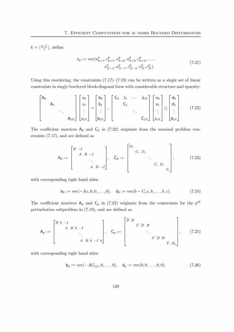
7. Efficient Computation for ∞–norm Bounded Disturbances
k = bp−1l c, define:
xp := vec(upk+1, c
pk+1, x
pk+2, u
pk+2, c
pk+2, . . . ,
xpN−1, u
pN−1, c
pN−1, x
pN , cp
N ).(7.21)
Using this reordering, the constraints (7.17)–(7.19) can be written as a single set of linear
constraints in singly-bordered block-diagonal form with considerable structure and sparsity:
A0
A1
. . .
AlN
x0
x1
...
xlN
=
b0
b1
...
blN
,
C0 J1 · · · JlN
C1
. . .
ClN
x0
x1
...
xlN
≤
d0
d1
...
dlN
. (7.22)
The coefficient matrices A0 and C0 in (7.22) originate from the nominal problem con-
straints (7.17), and are defined as
A0 :=
B −I
A B −I
. . .
A B −I
, C0 :=
Dc
Cc Dc
. . .
Cc Dc
Yc
, (7.23)
with corresponding right hand sides
b0 := vec(−Ax, 0, 0, . . . , 0), d0 := vec(b− Ccx, b, . . . , b, z). (7.24)
The coefficient matrices Ap and Cp in (7.22) originate from the constraints for the pth
perturbation subproblem in (7.19), and are defined as
Ap :=
B 0 −I
A B 0 −I
. . .
A B 0 −I 0
, Cp :=
D H
C D H
. . .
C D H
Y Hf
, (7.25)
with corresponding right hand sides
bp := vec(−AG(j), 0, . . . , 0), dp := vec(0, 0, . . . , 0, 0). (7.26)
120

7.3 Interior-Point Method for Robust Control
The coupling matrices Jp in (7.22) are then easily constructed from the coupling equa-
tion (7.18).
Remark 7.4. It is possible to define, in a fairly obvious way, a problem structure akin to
that in (7.16)–(7.19) for the general norm-bounded discussed in Section 6.2.3 via introduc-
tion of states in a similar manner. A similar statement can be made about the general
polytopic disturbance case discussed in Section (6.2.2); however, in the latter case the per-
turbation subproblems (7.19) require an additional coupling constraint for the subproblems
associated with each stage.
7.3 Interior-Point Method for Robust Control
In this section we demonstrate that, using a primal-dual interior-point solution technique,
the quadratic program defined in (7.16)–(7.19) is solvable in an amount of time that is
cubic in the horizon length N at each iteration, when n + m is dominated by N ; this situ-
ation is common, for example, in the rapidly growing number of aerospace and automotive
applications of predictive control [Mac02, Sec. 3.3][QB03]. This is a major improvement
on the O(N6) work per iteration associated with the compact (dense) formulation (7.2),
or the equivalent problem (7.5); cf. Remark 7.1. This computational improvement comes
about due to the improved structure and sparsity of the problem. Indeed, akin to the situ-
ation in [RWR98], we will show that each subproblem in the QP (7.16)–(7.19) has the same
structure as that of an unconstrained optimal control problem without disturbances.
7.3.1 General Interior-Point Methods
We first outline some of the general properties of interior-point solution methods by con-
sidering the general constrained quadratic optimization problem
minθ
1
2θ>Qθ subject to Aθ = b, Cθ ≤ d, (7.27)
where the matrix Q is positive semidefinite. An optimal solution θ for this system exists
if and only if the Karush-Kuhn-Tucker conditions are satisfied, i.e. there exist additional
121

7. Efficient Computation for ∞–norm Bounded Disturbances
vectors π, λ and z satisfying the following conditions:
Qθ + A>π + C>λ = 0 (7.28a)
Aθ − b = 0 (7.28b)
−Cθ + d− z = 0 (7.28c)
(λ, z) ≥ 0 (7.28d)
λ>z = 0. (7.28e)
The variables λ and z in (7.28) will be referred to as the Lagrange multipliers and slack
variables, respectively. In primal-dual interior point methods [Wri97], the central path is
defined as the set of parameters (θ, π, λ, z) satisfying (7.28a)–(7.28d), with the complemen-
tarity condition (7.28e) relaxed, for each element i, to λizi = µ, where µ > 0 parameterizes
the path. This guarantees that λ and z are strictly positive vectors. The central path
converges to a solution of (7.28) as µ ↓ 0 if such a solution exists.
The constraints λizi = µ can be rewritten in a slightly more convenient form by defining
diagonal matrices Λ and Z such that
Λ =
λ1
. . .
λn
, and Z =
z1
. . .
zn
, (7.29)
so that the relaxed complementarity condition becomes ΛZ1 = µ1. Primal-dual interior-
point algorithms search for a solution to the KKT conditions (7.28) by producing a sequence
of iterates (θκ, πκ, λκ, zκ) which approximate the central path solution at some µκ > 0.
These iterates are updated via repeated solution of a set of Newton-like equations of the
form
Q A> C>
A
C I
Z Λ
∆θ
∆π
∆λ
∆z
= −
rQ
rA
rC
rZ
, (7.30)
where the residuals (rQ, rA, rC) take the values of the left-hand sides of (7.28a)–(7.28c)
respectively, evaluated at the current values (θκ, πκ, λκ, zκ), and the matrices (Z, Λ) are
formed from the current iterates (zκ, λκ) as in (7.29). The residual vector rZ is typically
defined as rZ = (ΛZ1 − 1µ), where µ is chosen such that µ ∈ (0, µκ). Once the linear
122

7.3 Interior-Point Method for Robust Control
system (7.30) has been solved, the solution is updated as
(θκ+1, πκ+1, λκ+1, zκ+1)← (θκ, πκ, λκ, zκ) + α(∆θ, ∆π, ∆λ, ∆z),
where α > 0 is chosen to maintain strict positivity of λk+1 and zk+1, and the path parameter
µκ is updated to some µκ+1 ∈ (0, µκ). The particular method for selecting the parameters µ
and α at each iteration depends on the specific interior-point algorithm employed; the reader
is referred to [Wri97] for a thorough review.
Since all such methods maintain the strict inequalities (λ, z) > 0 at each iteration as µ ↓ 0,
the matrices Λ and Z are guaranteed to remain full rank, and the system of equations
in (7.30) can be simplified through elimination of the variables ∆z to form the reduced
system
Q A> C>
A
C −Λ−1Z
∆θ
∆π
∆λ
= −
rQ
rA(
rC − Λ−1rZ
)
. (7.31)
Since the number of interior-point iterations required in practice is only weakly related to
the number of variables [Wri97], the principal consideration is the time required to factor
the Jacobian matrix (i.e. the matrix on the left-hand-side), and solve the linear system
in (7.31). In the remainder of this chapter we focus on the development of an efficient
solution procedure for this linear system when the problem data for the QP (7.27) is defined
by the problem (7.16)–(7.19).
7.3.2 Robust Control Formulation
For the robust optimal control problem described in (7.16)–(7.19), the system of equations
in (7.31) can be arranged to yield a highly structured set of linear equations through ap-
propriate ordering of the primal and dual variables and their Lagrange multipliers at each
stage. As will be shown, this ordering enables the development of an efficient solution
procedure for the linear system in (7.31).
We use λi and λN to denote the Lagrange multipliers for the constraints (7.17b) and (7.17c)
in the nominal system, and zi and zN for the corresponding slack variables. We similarly
use λpi and λp
N to denote the multipliers in (7.19d) and (7.19e) for the pth perturbation
subproblem, with slack variables zpi and zp
N . We use πi and πpi to denote the dual variables
for (7.17) and (7.19).
123

7. Efficient Computation for ∞–norm Bounded Disturbances
The linear system (7.31), defined for the particular robust control problem (7.16)–(7.19), can
then be reordered to form a symmetric, block-bordered, banded diagonal set of equations by
interleaving the primal and dual variables within the nominal and perturbed problems, while
keeping the variables from each subproblem separate. If the pth perturbation subproblem
corresponds to a unit disturbance at some stage k = b p−1l c, then the components of the
system of equations (7.31) corresponding to the nominal variables and the variables for the
pth perturbation subproblem are coupled at all stages after k.
Considering for the moment only that part of (7.19) corresponding to the first perturbation
problem (with p = 1), this reordering yields the coupled linear system
R D>c B>
Dc −Σ0 0
B 0 0 −I
−I Q 0 C>c A>
0 R D>c B>
Cc Dc −Σ1 0 I
A B 0 0 −I
−I Q 0 C>c A>
0 R D>c B>
Cc Dc −Σ2 0 I
A B 0. . .
. . .. . . P Y>c
Yc −ΣN I
0 0 D> B>
I 0 0 H> 0
D H −Σ11 0
B 0 0 0 −I
−I 0 0 0 C> A>
0 0 0 D> B>
I 0 0 0 H> 0
C D H −Σ12 0
A B 0 0. . .
. . .. . . 0 0 Y>
I 0 0 H>f
Y Hf −Σ1N
∆v0
∆λ0
∆π0
∆x1
∆v1
∆λ1
∆π1
∆x2
∆v2
∆λ2...
∆xN
∆λN
∆u11
∆c11
∆λ11
∆π11
∆x12
∆u12
∆c12
∆λ12.
.
.
∆x1N
∆c1N
∆λ1N
=
rv0
rλ0
rπ0
rx1
rv1
rλ1
rπ1
rx2
rv2
rλ2...
rxN
rλN
ru11
rc11
rλ11
rπ11
rx12
ru12
rc12
rλ12
.
.
.
rx1
N
rc1N
rλ1
N
.
(7.32)
The diagonal matrices Σi and Σpi in (7.32) correspond to the matrix products Λ−1Z in
(7.31), and are defined as
Σi := (Λi)−1Zi, ∀i ∈ Z[0,N ] (7.33)
Σpi := (Λp
i )−1Zp
i , ∀i ∈ Z[k+1,N ], (7.34)
where the matrices Λi, Λpi , Zi, and Zp
i are diagonal matrices formed from the Lagrange
124

7.3 Interior-Point Method for Robust Control
multipliers and slack variables λi, λpi , zi and zp
i from the nominal and perturbation sub-
problems.
If all of the perturbation problems (7.19) are incorporated into a linear system of the
form (7.32), the result is a system of equations whose coefficient matrix can be partitioned
into block-bordered form as
A J1 J2 · · · JlN
J>1 B1
J>2 B2
.... . .
J>lN BlN
xA
x1
x2
...
xlN
=
bA
b1
b2
...
blN
, (7.35)
where the banded matrix A is derived from the coefficients in the nominal problem (7.17),
the banded matrices Bp are derived from the lN perturbation subproblems (7.19), and the
matrices Jp represent the coupling between the systems. The vectors bA, bp, xA, and xp
(which should not be confused with the stacked sequence of state vectors x) are constructed
from the primal and dual variables and residuals using the ordering in (7.32). The matrices
Jp are constructed from identity matrices coupling the rows of A that contain the Σi terms
with the columns of Bp that contain the H terms. It should of course be noted that for the
matrix Bp, corresponding to a unit disturbance at stage k = b p−1l c, terms from stages prior
to stage k + 1 are not required.
7.3.3 Solving for an Interior-Point Step
We can now estimate the solution time for the robust optimization problem (7.16)–(7.19) by
demonstrating that the linear system in (7.35) can be solved in O((m + n)3N3) operations.
We recall that, in practice, the number of interior-point iterations is only weakly dependent
on the size of the problem [Wri97]. Throughout this section, we make the simplifying
assumption that the number of constraints s and sf defining Z and Xf are O(m+n) and
O(n), respectively.
We first require the following preliminary results, proofs for which can be found in the
appendix to this chapter.
Lemma 7.5. For the robust control problem (7.16)–(7.19), the Jacobian matrix in (7.32)
is full rank.
125

7. Efficient Computation for ∞–norm Bounded Disturbances
Lemma 7.6. The sub-matrices Bp arising from the perturbation subproblems in (7.35) are
full rank. Additionally, recalling that k = b p−1l c,
i. A solution to the linear system Bpxp = bp can be found in O(
(m+n)3(N − k + 1))
operations.
ii. If a solution to (i) above has been found, then a solution for each additional right hand
side requires O(
(m+n)2(N − k + 1))
operations.
Remark 7.7. Note that each of the blocks Bp on the diagonal of (7.35) is banded and
symmetric indefinite. Several methods exist for the stable construction of Cholesky-like de-
compositions of symmetric indefinite matrices into factors of the form LDL> [BKP76], and
efficient algorithms for performing this factorization for sparse matrices are freely available
[DER86, HSL02]. However, it is generally not possible to guarantee that the banded struc-
ture of an indefinite matrix, such as Bp, will be exploited using these methods if symmetry
and stability of the factorization are to be preserved. Instead, the special structure of the
matrices Bp allows us to employ a specialized technique for solution of the linear system
Bpxp = bp based on a Riccati recursion [Ste95, RWR98] in the proof of Lemma 7.6 in
Appendix 7.A.2.
We can now demonstrate that it is always possible to solve the linear system (7.35) in
O((m+n)3N3) operations.
Theorem 7.8. For the robust optimal control problem (7.16)–(7.19), each primal-dual in-
terior point iteration requires no more than O((m+n)3N3) operations.
Proof. The linear system (7.35) can be factored and solved using a Schur complement
technique, so that
xA
x1
x2
...
xlN
=
I
− B−11 J>
1 I
− B−12 J>
2 I
.... . .
−B−1lN J>
lN I
∆−1
B−11
B−12
. . .
B−1lN
I −J1B−11 −J1B
−12 . . . −JlNB−1
lN
I
I
. . .
I
bA
b1
b2
...
blN
,
with
∆ := A−lN∑
p=1
JpB−1p J>
p .
where, by virtue of Lemma 7.5, the matrix ∆ is always full rank [HJ85, Thm. 0.8.5]. The
126

7.3 Interior-Point Method for Robust Control
O((m+n)3N3) complexity bound can then be attained by solving (7.35) using the following
procedure:
Operation Complexity
solve: xp = B−1p bp ∀p ∈ Z[1,lN ] lN · O((m+n)3N) (7.36a)
Sp = Jp
(
B−1p J>
p
)
∀p ∈ Z[1,lN ] lN · O((m+n)3N2) (7.36b)
factor: ∆ = A−lN∑
p=1
Sp lN · O((m+n)N) (7.36c)
= L∆D∆L>∆ O((m+n)3N3) (7.36d)
solve: zA = bA −lN∑
p=1
(Jpxp), lN · O((m+n)N) (7.36e)
xA = (L>∆)−1(D−1
∆ (L−1∆ zA)), O((m+n)2N2) (7.36f)
zp = J>p xA, ∀p ∈ Z[1,lN ] lN · O((m+n)N) (7.36g)
xp = xp − B−1p zp. ∀p ∈ Z[1,lN ] lN · O((m+n)2N). (7.36h)
The complexity of the solution to the linear system (7.36a) follows from Lemma 7.6(i). The
complexity of the solution to (7.36b) and (7.36h) follows from Lemma 7.6(ii), where each
of the matrices J>p in (7.36b) have O((m + n)N) nonzero columns.
Remark 7.9. In the solution procedure (7.36), it is important to note that since the cou-
pling matrices Ji have no more than a single 1 on every row and column, matrix products
involving left or right multiplication by Ji or J>i do not require any floating point operations
to calculate. The reader is referred to [BV04, App. C] for a more complete treatment of
complexity analysis for matrix operations.
Remark 7.10. If the solution procedure (7.36) is employed, then the robust optimization
problem is an obvious candidate for parallel implementation2. However, it is generally
not necessary to hand implement the suggested variable interleaving and block factorization
procedure to realize the suggested block-bordered structure in (7.35) and O((m + n)3N3)
solution time, as any reasonably efficient sparse factorization code can be expected to perform
similar steps automatically; see [DER86]. Note that the “arrowhead” structure in (7.35)
should be reversed (i.e. pointing down and to the right) in order for direct LDL> factorization
to produce sparse factors.
2Note that if a parallel scheme is employed to factor the lN matrices Bp, the overall complexity of O(N3)is not reduced – it would still require O(N3) operations to factor the dense matrix ∆.
127

7. Efficient Computation for ∞–norm Bounded Disturbances
Remark 7.11. Recalling the discussion of soft constraint handling in Section 6.3.1 and
Remark 7.2, it is easy to show that the inclusion of soft constraints does not qualitatively
alter the complexity results of Theorem 7.8, since the inclusion of such constraints amounts
only to a modification of the matrix A (and thus of the dense matrix ∆) in (7.36c), and
does not effect the complexity of any of the operations involving the banded matrices Bi.
7.4 Numerical Results
Two sparse QP solvers were used to evaluate the proposed formulation. The first, OOQP
[GW03], uses a primal-dual interior-point approach configured with the sparse factorization
code MA27 from the HSL library [HSL02] and the OOQP version of the multiple-corrector
interior-point method of Gondzio [Gon96].
The second sparse solver used was the QP interface to the PATH [DF95] solver. This
code solves mixed complementarity problems using an active-set method, and hence can
be applied to the stationary conditions of any quadratic program. Note that since we are
dealing with convex QPs, each optimization problem and its associated complementarity
system have equivalent solution sets.
All results reported in this section were generated on a single processor machine with a
3 GHz Pentium 4 processor and 2GB of RAM. We restrict our attention to sparse solvers
as the amount of memory required in the size of the problems considered is prohibitively
large for dense factorization methods.
A set of test cases was generated to compare the performance of the two sparse solvers
using the (M,v) formulation in (7.2) and the decomposition-based method of Section 7.2.
Each test case is defined by its number of states n and horizon length N . The remaining
problem parameters were chosen using the following rules:
• There are twice as many states as inputs.
• The constraint sets W , Z and Xf represent randomly selected symmetric bounds on
the states and inputs subjected to a random similarity transformation.
• The state space matrices A and B are randomly generated, with (A, B) controllable,
and with A potentially unstable.
• The dimension l of the generating disturbance is chosen as half the number of states,
with randomly generated G of full column rank.
• All test cases have feasible solutions. The initial state is selected such that at least
some of the inequality constraints in (7.17b) are active at the optimal solution.
128

7.4 Numerical Results
The average computational times required by each of the two solvers for the two problem
formulations for a range of problem sizes are shown in Table 7.1. Each entry represents the
average of ten test cases, unless otherwise noted. It is clear from these results that, as ex-
Table 7.1: Average Solution Times (sec)(M,v) Decomposition
Problem Size OOQP PATH OOQP PATH
2 states, 4 stages 0.004 0.004 0.005 0.0052 states, 8 stages 0.020 0.010 0.016 0.0192 states, 12 stages 0.061 0.027 0.037 0.0522 states, 16 stages 0.172 0.091 0.072 0.1982 states, 20 stages 0.432 0.123 0.132 1.431
4 states, 4 stages 0.024 0.026 0.018 0.0244 states, 8 stages 0.220 0.316 0.099 0.3574 states, 12 stages 0.969 1.162 0.264 2.0194 states, 16 stages 3.755 17.50 0.576 16.634 states, 20 stages 11.67 41.45 1.047 22.26
8 states, 4 stages 0.667 1.282 0.136 0.2618 states, 8 stages 7.882 81.50 0.858 14.898 states, 12 stages 46.97 257.9† 2.81 183.8†
8 states, 16 stages 189.75 2660† 6.781 288.9†
8 states, 20 stages 620.3 x 13.30 x
12 states, 4 stages 6.292 75.608 0.512 5.04412 states, 8 stages 132.1 1160† 4.671 388.9†
12 states, 12 stages 907.4 x 14.08 x12 states, 16 stages x x 37.99 x12 states, 20 stages x x 82.06 x
x – Solver failed all test cases† – Based on limited data set due to failures
pected, the decomposition-based formulation can be solved much more efficiently than the
original (M,v) formulation for robust optimal control problems of nontrivial size, and that
the difference in solution times increases dramatically with increased problem dimension.
Additionally, the decomposition formulation seems particularly well suited to the interior-
point solver (OOQP), rather than the active set method (PATH). Nevertheless we expect
the performance of active set methods to improve relative to interior-point methods when
solving a sequence of similar QPs that would occur in a receding horizon control scheme,
where a good estimate of the optimal active set is typically available at the start of compu-
tation. That is, interior-point methods are particularly effective in “cold start” situations,
while the efficiency of active set methods is likely to improve given a “warm start”.
129
7. Efficient Computation for ∞–norm Bounded Disturbances
Figure 7.1 shows that the interior-point solution time increases cubicly with horizon length
for randomly generated problems with 2, 4, 8 and 12 states. The performance closely
matches the predicted behavior described in Section 7.2. For the particular problems shown,
the number of iterations required for the OOQP algorithm to converge varied from 12 to
20 over the range of horizon lengths and state dimensions considered. The total number of
interior-point iterations required to solve each problem as a function of horizon length is
shown in Figure 7.2
7.5 Conclusions
In this chapter we have derived a highly efficient computational method for calculation of
affine state feedback policies for robust control of constrained systems with bounded dis-
turbances. This is done by exploiting the structure of the underlying optimization problem
and deriving an equivalent problem with considerable structure and sparsity, resulting in
a problem formulation that is particularly suited to an interior-point solution method. As
a result, the robustly stabilizing receding horizon control law proposed in Chapter 4 is
practically realizable, even for systems of significant size or with long horizon lengths.
In Section 7.3 we proved that, when applying an interior-point solution technique to our
robust optimal control problem, each iteration of the method can be solved using a number
of operations proportional to the cube of the control horizon length. We appeal to the
Riccati based factorization technique in [Ste95, RWR98] to support this claim. However,
it should be stressed that the results in Section 7.4, which demonstrate this cubic-time
behavior numerically, are based on freely available optimization and linear algebra packages
and do not rely on any special factorization methods.
A number of open research issues remain. It may be possible to further exploit the structure
of the control problem discussed in this chapter by developing specialized factorization
algorithms for the factorization of each interior-point step, e.g. through the parallel block
factorization procedure alluded to in Remark 7.10.
It is also possible to extend, in a fairly obvious way, the results of this chapter to certain
of the other H2 control problems for various disturbance classes proposed in Chapter 6. Of
particular interest, however, would be an extension of the results presented here allowing
the efficient solution of the various semidefinite programming problems arising in Chapter 6
in relation to constrained H∞ control problems.
130
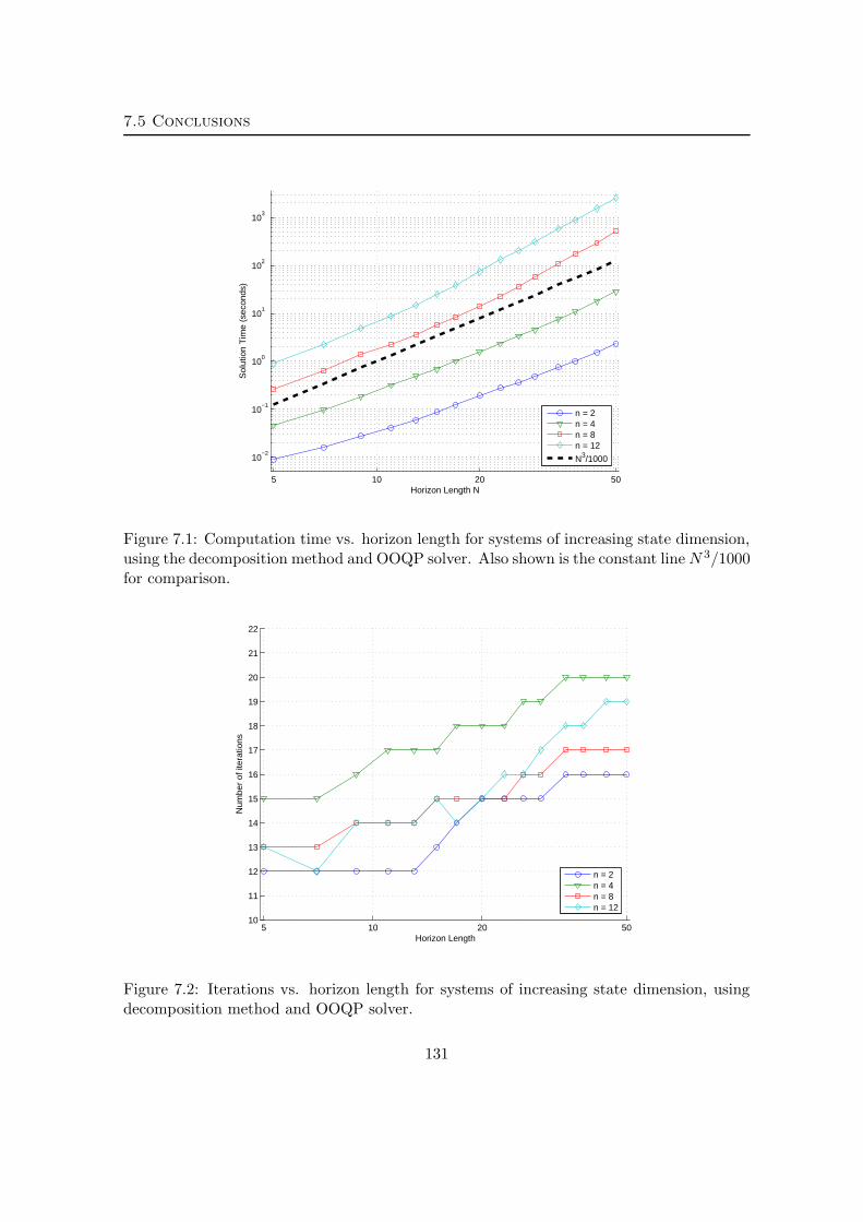
7.5 Conclusions
5 10 20 50
10−2
10−1
100
101
102
103
Horizon Length N
Sol
utio
n T
ime
(sec
onds
)
n = 2n = 4n = 8n = 12
N3/1000
Figure 7.1: Computation time vs. horizon length for systems of increasing state dimension,using the decomposition method and OOQP solver. Also shown is the constant line N 3/1000for comparison.
5 10 20 5010
11
12
13
14
15
16
17
18
19
20
21
22
Horizon Length
Num
ber
of it
erat
ions
n = 2n = 4n = 8n = 12
Figure 7.2: Iterations vs. horizon length for systems of increasing state dimension, usingdecomposition method and OOQP solver.
131
7. Efficient Computation for ∞–norm Bounded Disturbances
7.A Proofs
7.A.1 Rank of the Robust Control Problem Jacobian (Proof of Lemma 7.5)
We demonstrate that the Jacobian matrix defined in (7.32) is always full rank. Recalling
the discussion in Section 7.3.1, for any quadratic program the Jacobian matrix is full rank
if the only solution to the system
Q A> C>
A 0 0
C 0 −Σ
∆θ
∆π
∆λ
=
0
0
0
(7.37)
satisfies ∆θ = 0, ∆π = 0, and ∆λ = 0, where Σ := Λ−1Z Â 0, Q º 0 and the coefficient
matrices A and C come from the equality and inequality constraints of the QP respectively
(cf. (7.27)). From the first two rows of this system,
∆θ>Q∆θ + (∆θ>A>)∆π + ∆θ>C>∆λ = ∆θ>Q∆θ + ∆θ>C>∆λ = 0. (7.38)
Incorporating the final block row, C∆θ = Σ∆λ, we have
∆θ>Q∆θ + ∆λ>Σ∆λ = 0. (7.39)
Since Q º 0 for a convex QP and Σ Â 0 for a strictly interior point, we conclude that
∆λ = 0. We next make use of the following matrix condition, which is easily verified:
Fact 7.12. The matrix[
X Y0 Z
]
is full column rank for any Y if both X and Z are full column
rank.
Since ∆λ = 0 always holds, sufficient conditions to guarantee ∆θ = 0 and ∆π = 0 in (7.37)
are that:
(i) A is full row rank.
(ii)[
AC
]
is full column rank.
For the quadratic program defined by the robust control problem (7.17)–(7.19), the equality
and inequality constraints are defined as in (7.22). For this convex QP, it is straightforward
to show that the above rank conditions on A and C are equivalent to requiring that:
(i) Each of the matrices A0, A1, . . . , AlN is full row rank.
132

7.A Proofs
(ii) Each of the matrices[
A0C0
]
,[
A1C1
]
, . . . ,[
AlN
ClN
]
is full column rank.
The condition (ii) is derived by noting that, for the particular problem (7.17)–(7.19), the
general rank condition on[
AC
]
is equivalent to requiring that the matrix
C0 J1 J2 . . . JlN
A0
C1
A1
C2
A2
. . .
ClN
AlN
is full column rank, which reduces to (ii) upon repeated application of Fact 7.12 above to
eliminate the coupling terms Jp. If A7.1(iii) holds so that Dc is full column rank, then
both of these rank conditions are easily verified by examination of the definitions in (7.23)
and (7.25). The Jacobian matrix for the QP defined in (7.17)–(7.19) is thus full rank, and
it remains full rank if its rows and columns are reordered as in (7.32).
7.A.2 Solution of Bpxp = bp via Riccati Recursion (Proof of Lemma 7.6)
We demonstrate that the system of equations Bpxp = bp has a unique solution for every
bp, where Bp, xp and bp are defined as
Bp :=
0 0 D> B>
0 0 H> 0
D H −Σpk+1
0
B 0 0 0 −I
−I 0 0 0 C> A>
0 0 0 D> B>
0 0 0 H> 0
C D H −Σpk+2
0
A B 0 0. . .
. . .. . . 0 0 Y>
0 0 H>f
Y Hf −ΣpN
, (7.40a)
xp :=vec(∆upk+1, ∆cp
k+1, ∆λpk+1, ∆πp
k+1, ∆xpk+2, ∆up
k+2, ∆cpk+2, ∆λp
k+2, . . . , ∆xpN , ∆cp
N , ∆λpN ),
bp :=vec( rupk+1 , rcp
k+1 , rλpk+1 , rπp
k+1 , rxpk+2 , rup
k+2 , rcpk+2 , rλp
k+2 , . . . , rxpN , rcp
N , rλpN )
133

7. Efficient Computation for ∞–norm Bounded Disturbances
and k = bp−1l c, and that this solution is obtainable in O((m + n)3N) operations. We
first perform a single step of block elimination on the variables ∆λpi and ∆cp
k+1, so that
the resulting linear system is solvable via specialized methods based on Riccati recursion
techniques [Ste95, RWR98] (see also related results in [DB89] for the unconstrained case).
It is straightforward to eliminate the terms ∆λpi and ∆cp
i from each of the subproblems,
yielding a linear system Bpxp = bp. The coefficient matrix Bp is:
Bp :=
Rpk+1
B>
B 0 −I
−I Qpk+2
Mpk+2
A>
(Mpk+2
)> Rpk+2
B>
A B 0 −I
−I Qpk+3
Mpk+3
A>
(Mpk+3
)> Rpk+3
B>
A B
. . .. . .
. . . QpN
(7.41)
where, for stages i ∈ Z[k+1,N−1]:
Φpi := H>(Σp
i )−1H (7.42a)
Θpi := (Σp
i )−1 − (Σp
i )−1H(Φp
i )−1H>(Σp
i )−1 (7.42b)
Qpi := C>Θp
i C (7.42c)
Rpi := D>Θp
i D (7.42d)
Mpi := C>Θp
i D, (7.42e)
and for stage N :
ΦpN := H>
f (ΣpN )−1Hf (7.42f)
ΘpN := (Σp
N )−1 − (ΣpN )−1Hf (Φp
N )−1H>f (Σp
N )−1 (7.42g)
QpN := Y>Θp
N Y. (7.42h)
The vectors xp and bp are defined as:
xp := vec(∆upk+1, ∆πp
k+1, ∆xpk+2, ∆up
k+2, ∆πpk+2, . . . , ∆xp
N ) (7.43)
bp := vec( rupk+1 , rπp
k+1 , rxpk+2 , rup
k+2 , rπpk+2 , . . . , rxp
N ) , (7.44)
134

7.A Proofs
where, for stages i ∈ Z[k+1,N−1]:
rxpi := rxp
i + C(
Θpi r
λpi − (Σp
i )−1H(Φp
i )−1rcp
i
)
(7.45a)
rupi := rup
i + D(
Θpi r
λpi − (Σp
i )−1H(Φp
i )−1rcp
i
)
, (7.45b)
and, for stage N :
rxpN := rxp
N + Y(
ΘpNrλp
N − (ΣpN )−1Hf (Φp
N )−1rcpN
)
. (7.45c)
Remark 7.13. The matrix Bp is equivalent to the KKT matrix for the unconstrained con-
trol problem:
minuk+1,...,uN−1,
xk+1,...,xN
1
2x>NQp
NxN +N−1∑
i=(k+1)
1
2(x>iQ
pi xi + u>iR
pi ui + 2xiM
pi ui)
(7.46)
subject to:
xk = G(j), (7.47a)
xi+1 = Axi + Bui, ∀i ∈ Z[k+1,N−1]. (7.47b)
Lemma 7.14. Each of the matrices Rpi , Qp
i and QpN are positive semidefinite. If A7.1
holds, then Rpi is positive definite.
Proof. Recall that the matrix Θpi is defined as
Θpi = (Σp
i )−1 − (Σp
i )−1H
(
H ′(Σpi )
−1H)−1
H>(Σpi )
−1 (7.48)
Partition the diagonal and positive definite matrix Σpi into Σp
i =[
Σ1 00 Σ2
]
. Recalling that
H := −[
II
]
, Θpi can be written as
Θpi =
[
Σ−11 − Σ−1
1 (Σ−11 + Σ−1
2 )−1Σ−11 −Σ−1
1 (Σ−11 + Σ−1
2 )−1Σ−12
−Σ−12 (Σ−1
1 + Σ−12 )−1Σ−1
1 Σ−11 − Σ−1
2 (Σ−11 + Σ−1
2 )−1Σ−12
]
(7.49)
=
[
I
−I
]
(Σ1 + Σ2)−1[
I −I]
(7.50)
which is easily verified using standard matrix identities and the fact that the matrices Σ1
and Σ2 are diagonal.
135

7. Efficient Computation for ∞–norm Bounded Disturbances
Recalling that D :=[
Dc
−Dc
]
, it follows that Rpi is positive semidefinite since it can be written
as
Rpi = D>
[
I
−I
]
(Σ1 + Σ2)−1[
I −I]
D (7.51)
= 4D>(Σ1 + Σ2)−1D º 0. (7.52)
If A7.1(iii) holds so that Dc is full column rank, then Rpi is positive definite. A similar
argument establishes the result for Qpi and Qp
N .
We are now in a position to prove Lemma 7.6. Since Rpi is positive definite and Qp
i and
QpN are positive semidefinite, the linear system Bpxp = bp (and consequently the original
system Bpxp = bp) has a unique solution that can found in O((m+n)3(N−k+1)) operations
using the Riccati recursion procedure described in [Ste95, RWR98]. Once such a solution has
been obtained, a solution for each additional right hand side requires O(
(m+n)2(N−k+1))
operations [RWR98, Sec. 3.4]. We note that in [RWR98] the Riccati factorization procedure
is shown to be numerically stable, and that similar arguments can be used to show that
factorization of (7.41) is also stable.
136

Chapter 8. Constrained Output Feedback
In this chapter we extend the results for the state feedback problem considered in the ma-
jority of this dissertation to the output feedback case. The results presented here broadly
parallel the results of Chapter 3; a class of feedback policies will be introduced that guar-
antees constraint satisfaction for all time for a linear system subject to convex constraints
and bounded disturbances and output measurement errors, and that can be computed via
the solution of a convex optimization problem.
8.1 Problem Definition
Throughout, we consider the following discrete-time linear time-invariant system:
x+ = Ax + Bu + w (8.1)
y = Cx + η (8.2)
where x ∈ Rn is the system state at the current time instant, x+ is the state at the next
time instant, u ∈ Rm is the system input, w ∈ R
n is a disturbance, y ∈ Rr is the system
output and η ∈ Rr is a measurement error. We will assume that, at each time step, a
measurement of the output y is available, but a measurement of the state x is not.
We assume that the disturbances w are unknown but contained within a compact set W
containing the origin, and that the measurement errors η are unknown but contained in a
compact set H ⊂ Rr, also containing the origin. We will also assume that an initial state
estimate s ∈ Rn is provided along with a compact estimation error set E , such that the
state x is initially known to satisfy x ∈ s ⊕ E .
As in Chapter 3, the system is subject to mixed constraints on the states and inputs, so
that a design goal is to guarantee that (x, u) ∈ Z ∈ Rn × R
m for all time; note that such a
constraint may include constraints on the output y. For finite horizon problems, one may
137

8. Constrained Output Feedback
additionally specify some closed and convex target set XT which the state x must reach
after a fixed number of time steps.
We will only consider the problem of finding a feasible (i.e. constraint admissible) output
feedback control policy for the system (8.1)–(8.2), without regard to optimality. We make
use of the following assumptions about the system (8.1)–(8.2) throughout this chapter:
A8.1 (Standing Assumptions)
i. The pairs (A, B) and (C, A) are stabilizable and detectable respectively.
ii. The state and input constraint set Z ⊆ Rn × R
m is closed, convex, contains the origin
in its interior and is bounded in the inputs, i.e. there exists a bounded set B such that
Z ⊆ Rn ×B.
8.2 Control Policy and Observer Structure
As in the full state information case considered in Chapter 3, finding an arbitrary finite
horizon control policy that satisfies the constraints of the system (8.1)–(8.2) for all possible
uncertainty realizations is extremely difficult in general. As a result, we will restrict the
class of control policies considered to those in which each control input ui is affine in the
measurements y0, . . . , yi−1, i.e.
ui = gi +i−1∑
j=0
Ki,jyj , ∀i ∈ Z[0,N−1], (8.3)
and consider the problem of finding a policy in this form that is guaranteed to satisfy the
system constraints for all possible uncertainty realizations. Note that such a control policy
is the logical counterpart, in the output feedback case, to the class of state feedback policies
introduced in Section 3.2. For infinite horizon problems, we will consider the construction
of constraint admissible control laws based on receding horizon implementations of policies
in the form (8.3).
8.2.1 Observers and Terminal Sets
For infinite horizon problems, we will find it helpful to introduce a linear control law and
associated robust positively invariant set to serve as a target/terminal constraint in a manner
138

8.2 Control Policy and Observer Structure
similar to that used in Chapter 3 (cf. the assumptions of A3.2). The obvious extension
of A3.2 when implementing receding horizon controllers based on output feedback policies
in the form (8.3) is to define a feedback matrix Kf such that (A + BKfC) is Hurwitz, and
to find an associated robust positively invariant for the system (8.1)–(8.2) in closed loop
with the control law u = Kfy. However, the problem of finding such a Kf is generally
believed to be NP hard [BT97].
As an alternative, we specify a Luenberger type observer gain L such that
s+ = As + Bu + L(y − Cs) (8.4)
and define the state estimation error e ∈ Rn as e := x− s, such that
e+ = (A− LC)e− Lη + w, (8.5)
where s+ and e+ represent a state estimate and estimation error at the next time instant.
In conjunction with this observer, we define a closed and convex target/terminal constraint
set Xf for the joint state estimate and estimation error, so that a design goal (for finite
horizon problems) will be to drive the system (8.4)–(8.5) to satisfy (s, e) ∈ Xf at the end of
the planning horizon1. For receding horizon implementations, we will define Xf such that
it is robust positively invariant for the system (8.4)–(8.5) in closed loop with a stabilizing
control law of the form u = Kfs.
Note that if one only wishes to ensure that x ∈ XT for some target set XT at the end of a
finite planning horizon, then one can define
Xf := (s, e) | s + e ∈ XT . (8.6)
In such a case no observer is required, and nothing is gained or lost by specifying one.
However, in order to maintain consistency of notation throughout, we will use a target set
Xf as defined above with the understanding that it can be defined as in (8.6) if required.
Note that if it is known initially that x ∈ s ⊕ E , then the state at the next time instant
will be known to satisfy
x+ ∈ s+ ⊕ (A− LC)E ⊕W ⊕ (−L)H (8.7)
1This definition of the terminal constraint differs from that used in previous chapters, where Xf wasdefined as a constraint on the true state x, rather than on the joint state estimate and estimation error pair(s, e).
139

8. Constrained Output Feedback
if an observer of the form (8.4)–(8.5) is used. The main technical issue to be addressed in
this chapter is the problem of synthesizing a receding horizon control law from policies in
the form (8.3) that is both time-invariant and that can be calculated by solving a finite-
dimensional optimization problem. The difficulty of computing such a control law arises
mainly from the fact that given an initial estimation error set E of fixed complexity (e.g. one
characterized by a finite number of linear inequalities), the complexity of future state esti-
mation error sets generally increases without bound if one employs a linear state observer.
As will be shown, this problem can be circumvented via the use of an outer approximation
to the initial error set which is robust positively invariant in closed loop with the state
estimator.
Remark 8.1. Note that unlike in previous chapters, the disturbance input to the sys-
tem (8.1) is not multiplied by a matrix G, and the disturbances are drawn from a set W
containing the origin in its interior (note that the interior of the set GW might be empty if
G is not full row rank, even when W has nonempty interior). The reason for this distinc-
tion is twofold; first, the results to follow will require the construction of an invariant outer
approximation to the minimal robust positively invariant set for the error dynamics (8.5)
using the results of [RKKM04, RKKM05]. The methods for constructing such a set require
that W ⊕ (−L)H has nonempty interior. Second, the method to be proposed for defining
an invariant control law for the system (8.1) is based on a modification of W such that the
disturbance inputs to the system (8.1) are drawn from a slightly larger set with nonempty
interior; this method would be incompatible with any G that is not invertible.
8.2.2 Alternative Observer Schemes
In this chapter we propose a method for calculating robust finite horizon control policies
for the system (8.1)–(8.2), where the control input uk at each time k is determined as an
affine function of the measurements y0, . . . , yk−1. The decision not to allow the control
input uk to also depend on the measurement yk will be consistent with the choice of the
Luenberger form observer in (8.4) when developing the invariance results of Section 8.5.
As an alternative, one could employ a predictor-corrector type observer of the form
sk+1 = (I − LC)(Ask + Buk) + Lyk+1 (8.8a)
ek+1 = (I − LC)(Aek + wk)− Lηk+1, (8.8b)
when constructing an invariant terminal set. Such an observer would be consistent with a
140

8.2 Control Policy and Observer Structure
control policy where each input uk is modelled as an affine function of the measurements
y0, . . . , yk. Such an alternative formulation is not qualitatively different from the method
used here, and observers in both forms are in widespread use. Note that if one were to
employ an observer in the form (8.8) with H = 0, C = I and L = I, and were then
to define an affine control policy in y0, . . . , yk, then one would recover exactly the affine
state feedback control problem of Section 3.2.
We elect to use an observer of the form (8.4) primarily for consistency and convenience
of comparison with related work within the predictive control literature on output feed-
back [LK01, RH05, MRFA06]. Additionally, the proposed parameterization is slightly more
relaxed, since it does not require the measurement yk, which may not always be available,
to calculate uk. It should be stressed that use of the alternative state estimate and error
dynamics (8.8) would not by itself alleviate the main technical difficulties to be addressed
in Section 8.5.
Finally, this chapter will not directly address the issue of computational delay since this issue
can be adequately managed using available methods in the literature. For example, [Mac02,
Sec. 2.5] gives a procedure for transforming a system with computational delay into the
standard form considered in (8.1)–(8.4).
8.2.3 Notation
We will use of much of the notation introduced in Section 3.1.1, and further define stacked
versions of the state estimate, estimation error, output, and measurement error vectors
s ∈ Rn(N+1), e ∈ R
n(N+1), y ∈ RrN and η ∈ R
rN respectively, as
s :=
s0
s1
...
sN
, e :=
e0
e1
...
eN−1
, y :=
y0
y1
...
yN−1
, and η :=
y0
y1
...
yN−1
, (8.9)
where s0 := s and e0 := e denote the current values of the state estimate and estimation
error respectively, and si+1 := (A−LC)si +Bui +Lyi and ei+1 := (A−LC)ei−Lηi +wi for
all i ∈ Z[0,N−1]. The predicted measurements after i time instants are yi = C(si + ei) + ηi
for all i ∈ Z[0,N−1]. The actual values of the state, state estimate, estimation error, input
and output at time instant k are denoted x(k), s(k), e(k), u(k) and y(k), respectively.
We define a closed and convex set Z, appropriately constructed from Z and Xf , such that
141

8. Constrained Output Feedback
the constraints to be satisfied are equivalent to (s, e,u) ∈ Z, i.e.
Z :=
(s, e,u)
∣
∣
∣
∣
∣
(si + ei, ui) ∈ Z, ∀i ∈ Z[0,N−1]
(sN , eN ) ∈ Xf
. (8.10)
Note that, as with the set Xf , this definition of Z differs from that used in previous chapters
since it is defined in terms of the joint state estimate and estimation error sequences s and
e, rather than the sequence of true states x.
Define AL := (A − LC) and matrices Φ ∈ Rn(N+1)×n, Γ ∈ R
n(N+1)×nN , L ∈ RnN×rN and
C ∈ RnN×rN as
Φ :=
In
AL
A2L
...
ANL
, Γ :=
0 0 · · · 0
In 0 · · · 0
AL In · · · 0...
.... . .
...
AN−1L AN−2
L · · · In
,
L := IN ⊗ L, and C := [(IN ⊗ C) 0] respectively. Finally, define affine functions fe and fs
such that the vectors s and e can be written as
s =fs(s, e,u,w, η) := As + Bu + EL(Ce + η) (8.11)
e = fe(e,w, η) := Φe− ΓLη + Γw. (8.12)
Note that using these definitions, the state estimates s can alternatively be expressed di-
rectly as an affine function of y, i.e.
s = Φs + ΓBu + ΓLy. (8.13)
We define E to be the set of all compact subsets of Rn, and W to be the set of all compact
subsets of Rn containing the origin in their interior.
The reason for defining the sets E and W in this way is to allow for some flexibility in
subsequent control policy definitions, where the set of feasible policies will be defined in
terms of the disturbances and initial errors to which they are robust. We will typically
specify that the estimation error e and true initial state x are such that e ∈ E and x ∈ s⊕E ,for some E ∈ E, and that the disturbances w are unknown but drawn from some known set
W ∈W.
142
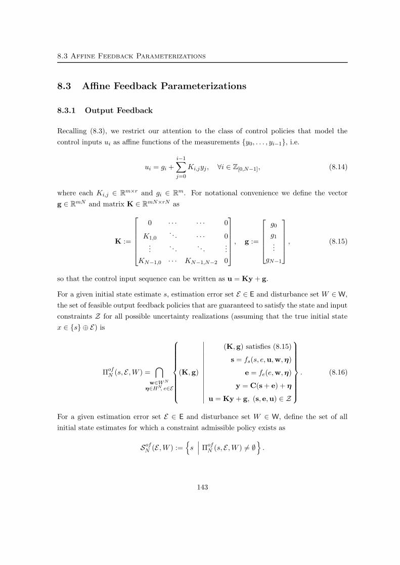
8.3 Affine Feedback Parameterizations
8.3 Affine Feedback Parameterizations
8.3.1 Output Feedback
Recalling (8.3), we restrict our attention to the class of control policies that model the
control inputs ui as affine functions of the measurements y0, . . . , yi−1, i.e.
ui = gi +i−1∑
j=0
Ki,jyj , ∀i ∈ Z[0,N−1], (8.14)
where each Ki,j ∈ Rm×r and gi ∈ R
m. For notational convenience we define the vector
g ∈ RmN and matrix K ∈ R
mN×rN as
K :=
0 · · · · · · 0
K1,0. . . · · · 0
.... . .
. . ....
KN−1,0 · · · KN−1,N−2 0
, g :=
g0
g1
...
gN−1
, (8.15)
so that the control input sequence can be written as u = Ky + g.
For a given initial state estimate s, estimation error set E ∈ E and disturbance set W ∈W,
the set of feasible output feedback policies that are guaranteed to satisfy the state and input
constraints Z for all possible uncertainty realizations (assuming that the true initial state
x ∈ s ⊕ E) is
ΠofN (s, E , W ) =
⋂
w∈W N
η∈HN, e∈E
(K,g)
∣
∣
∣
∣
∣
∣
∣
∣
∣
∣
∣
∣
∣
∣
(K,g) satisfies (8.15)
s = fs(s, e,u,w, η)
e = fe(e,w, η)
y = C(s + e) + η
u = Ky + g, (s, e,u) ∈ Z
. (8.16)
For a given estimation error set E ∈ E and disturbance set W ∈ W, define the set of all
initial state estimates for which a constraint admissible policy exists as
SofN (E , W ) :=
s∣
∣
∣ ΠofN (s, E , W ) 6= ∅
.
143

8. Constrained Output Feedback
Remark 8.2. It is important to recognize that for a finite horizon problem with a terminal
state constraint in the form xN ∈ XT , it is not necessary to specify an observer, and nothing
is gained or lost by doing so. For problems of this type, one can rewrite (8.16) as
ΠofN (s, E , W ) =
⋂
w∈W N
η∈HN, e∈E
(K,g)
∣
∣
∣
∣
∣
∣
∣
∣
∣
∣
∣
∣
∣
∣
(K,g) satisfies (8.15)
x = Ax + Bu + Ew
y = Cx + η, u = Ky + g
(xi, ui) ∈ Z, ∀i ∈ Z[0,N−1]
x = s + e, xN ∈ XT
, (8.17)
which is not related to any choice of observer, nor is the set SofN (E , W ). The advantage
of accounting explicitly for the action of a linear observer in defining the policy set (8.16)
is that it will allow us to construct an invariant receding horizon control law when the
constraint set Xf is defined as a robust positively invariant set for the system (8.4)–(8.5)
in closed loop with a linear feedback control law.
Remark 8.3. The feedback policy (8.14) includes the class of “pre-stabilizing” control poli-
cies in which the control is based on perturbations ciN−1i=0 to a fixed linear state feed-
back gain K, so that ui = ci + Ksi, since the estimated state si can be expressed as an
affine function of the measurements y0, . . . , yi−1 (cf. (8.13)). Such a scheme is com-
monly employed in conjunction with a stabilizing linear observer gain L for output feed-
back [LK01, RH05, YB05]. The method proposed can also be shown to subsume tube-based
schemes such as [MSR05, MRFA06] when the invariant sets defining the tube are based on
linear state feedback, though these methods also confer additional stability properties which
we do not address here. Finally, note that unlike the certainty-equivalence based method pro-
posed in [BR71], we do not combine the state estimation error set E with the disturbance
set W into a single lumped disturbance at each time step, but rather consider the effect of
the estimation error e ∈ E at the initial time propagated over the planning horizon.
Remark 8.4. As in the state feedback case considered in Chapter 3, the set ΠofN (s, E , W )
is nonconvex, in general, due to the nonlinear relationship between the estimated states s
and feedback gains K in (8.16).
144
8.3 Affine Feedback Parameterizations
8.3.2 Output Error Feedback
As an alternative to the parameterization (8.14), we consider a control policy parameterized as
ui = vi +
i−1∑
j=0
Mi,j(yj − Csj), ∀i ∈ Z[0,N−1] (8.18)
= vi +i−1∑
j=0
Mi,j(Cej + ηj), ∀i ∈ Z[0,N−1], (8.19)
where each Mi,j ∈ Rm×r and vi ∈ R
m. We further define the matrix M ∈ RmN×rN and
vector v ∈ RmN as
M :=
0 · · · · · · 0
M1,0 0 · · · 0...
. . .. . .
...
MN−1,0 · · · MN−1,N−2 0
, v :=
v0
v1
...
vN−1
, (8.20)
so that the control input sequence can be written as
u = M(y −Cs) + v (8.21)
= M(Ce + η) + v. (8.22)
By virtue of the relation (8.12), this control parameterization is affine in the unknown
parameters e, w and η. The control parameterization (8.19) is therefore the logical coun-
terpart, in the output feedback case, to the class of disturbance feedback policies introduced
in Section 3.3. For a given initial state estimate s, estimation error set E ∈ E and distur-
bance set W ∈ W, the set of feasible feedback policies that are guaranteed to satisfy the
system constraints for all possible uncertainty realizations (assuming that the true initial
state x ∈ s ⊕ E) is
ΠefN (s, E , W ) =
⋂
w∈W N
η∈HN, e∈E
(M,v)
∣
∣
∣
∣
∣
∣
∣
∣
∣
∣
∣
∣
∣
∣
(M,v) satisfies (8.20)
s = fs(s, e,u,w, η)
e = fe(e,w, η)
u = M(Ce + η) + v
(s, e,u) ∈ Z
. (8.23)
145
8. Constrained Output Feedback
For a given error set E ∈ E and disturbance set W ∈ W, define the set of all constraint
admissible initial state estimates to be
SefN (E , W ) :=
s∣
∣
∣Πef
N (s, E , W ) 6= ∅
. (8.24)
Remark 8.5. As in the affine output feedback case, the set SefN (E , W ) is independent of
any choice of observer for finite horizon problems with a terminal constraint in the form
xN ∈ XT (cf. Remark 8.2).
We next characterize two critical properties of the parameterization (8.19) which make
it attractive in application to control of the system (8.1), and which parallel the results
in Section 3.3 for the disturbance feedback case.
8.4 Convexity and Equivalence
8.4.1 Convexity and Closedness
We first establish convexity and closedness of the sets ΠefN (s, E , W ) and Sef
N (E , W ). Proof
of the following results closely parallels the proof of the corresponding results for the dis-
turbance feedback case in Section 3.4, and so will not be repeated here.
Theorem 8.6 (Convexity). For any E ∈ E, W ∈ W and s ∈ SefN (E , W ), the set of
constraint admissible feedback policies ΠefN (s, E , W ) is closed and convex. Furthermore,
the set of state estimates SefN (E , W ), for which at least one admissible affine output error
feedback policy exists, is also closed and convex.
Proposition 8.7 (Convexification of Uncertainty Sets). Given sets W ∈W and E ∈E, the sets Πef
N (s, W, E) and SefN (E , W ), defined in (8.23) and (8.24) respectively, are un-
changed if E, W and H are replaced with their convex hulls.
Corollary 8.8 (Polyhedral Sets). If the constraint sets Z and Xf are polyhedral and the
sets E, W and H are polytopes, then the set SefN (E , W ) is polyhedral and Πef
N (s, E , W ) is
polyhedral for each s ∈ SefN (E , W ).
146
8.4 Convexity and Equivalence
8.4.2 Equivalence of Affine Policy Parameterization
We next show that, as with the state and disturbance feedback parameterizations introduced
in Chapter 3, the two affine feedback policies introduced in this chapter are equivalent.
Theorem 8.9. Given any initial state estimation error set E ∈ E and any disturbance set
W ∈W, the sets SefN (E , W ) and Sof
N (E , W ) are equal. Additionally, given any s ∈ SofN (E , W ),
for any admissible (K,g) an admissible (M,v) can be found which yields the same state
and input sequence for all allowable disturbance sequences, and vice-versa.
Proof. SofN (E , W ) ⊆ Sef
N (E , W ): By definition, for any s ∈ SofN (E , W ), there exists a pair
(K,g) ∈ ΠofN (s, E , W ). A bit of algebra shows that, given any uncertainty realization e, η
and w, the input sequence u can be written as
u = ∆−1K [C(Ae + Ew) + η] + ∆−1(KCAs + g), (8.25)
where ∆ := (I −KCB), and the matrix ∆ is always invertible since KCB is strictly lower
triangular. Noting the identity C(Ae+Ew)+η = (I+CEL)(y−Cs), the input sequence u
can be written as
u = ∆−1K(I + CEL)(y −Cs) + ∆−1(KCAs + g).
A constraint admissible policy (M,v) ∈ SefN (E , W ) can then be found by selecting
M = ∆−1K(I + CEL), v = ∆−1(KCAs + g). (8.26)
Thus, s ∈ SefN (E , W ) for all s ∈ Sof
N (E , W ), so SofN (E , W ) ⊆ Sef
N (E , W ).
SefN (E , W ) ⊆ Sof
N (E , W ): By definition, for any s ∈ SefN (E , W ), there exists a pair (M,v) ∈
ΠefN (s, E , W ). Using the relation (8.13), the output error terms can be written as y−Cs =
(I −CΓL)y −CΦs−CΓBu, and the control input sequence u = M(y −Cs) + v as
u = ∆−1M(I −CΓL)y + ∆−1(v −MCΦs),
where ∆ := (I + MCΓB), and the matrix ∆ is always invertible since MCΓB is strictly
lower triangular. A constraint admissible policy (K,g) ∈ SofN (E , W ) can then be found by
147

8. Constrained Output Feedback
selecting
K = ∆−1M(I −CΓL), g = ∆−1(v −MCΦs). (8.27)
Thus, s ∈ SofN (E , W ) for all s ∈ Sef
N (E , W ), so SefN (E , W ) ⊆ Sof
N (E , W ).
Remark 8.10. A control policy based on the measurement prediction error terms (y −Cs)
was proposed in [vHB05], and independently in the context of robust optimization in [BBN06].
The latter gives an equivalence proof similar to that presented here, but without the inclusion
of a nonzero initial state estimate or observer dynamics. In the sequel, we make explicit
use of these error dynamics to derive conditions under which receding horizon control laws
based on the parameterization (8.19) can be guaranteed to satisfy constraints for the resulting
closed-loop system for all time.
8.5 Geometric and Invariance Properties
In this section, we characterize some of the geometric and invariance properties associated
with control laws synthesized from the feedback parameterization (8.19). We first require
the following assumption about the terminal constraint set Xf :
A8.2 (Terminal Constraint) For a given disturbance set W ∈ W, a state feedback gain
matrix Kf , observer gain L and terminal constraint set Xf have been chosen such that:
i. The matrices A + BKf and A− LC are Hurwitz.
ii. Xf is contained inside the set for which the constraints(
(s + e), u)
∈ Z are satisfied
under the control u = Kfs, i.e. Xf ⊆
(s, e)∣
∣
(
(s + e), Kfs)
∈ Z
.
iii. Xf is robust positively invariant for the closed-loop system s+ = (A+BKf )s+L(Ce+η)
and e+ = ALe−Lη+w, i.e. (s+, e+) ∈ Xf for all (s, e) ∈ Xf , all w ∈W and all η ∈ H.
Remark 8.11. If the set W × H is a polytope or affine map of a p-norm ball and the
constraints Z are polyhedral, then one can calculate an invariant set which satisfies the
conditions A8.2 by applying the techniques in [Bla99, KG98] to the augmented system
[
s+
e+
]
=
[
(A + BKf ) LC
0 (A− LC)
][
s
e
]
+
[
0 L
I −L
][
w
η
]
. (8.28)
148

8.5 Geometric and Invariance Properties
In general, one wishes to select the terminal set Xf such that it is a maximal invariant set,
so that the set ΠN (E , W ) is as large as possible. Alternatively, one can use the techniques
in [LK99] for calculating a target set of a given complexity.
Remark 8.12. If one wishes to employ the alternative observer scheme (8.8) in conjunc-
tion with a control policy of the form ui = gi+∑i
j=0 Ki,jyj, then construction of an invariant
terminal set Xf would need to be modified accordingly. One could, for example, replace the
augmented system (8.28) with the system
[
s+
e+
]
=
[
(A + BK) LC
0 (I − LC)A
][
s
e
]
+
[
LC L
(I − LC) −L
][
w
η
]
, (8.29)
and then employ all of the same methods suggested in Rem. 8.11 to calculate the set Xf .
8.5.1 Monotonicity of SofN (E ,W ) and Sef
N (E ,W )
Proposition 8.13 (Monotonicity). If A8.2 holds, then the following set inclusions hold
for any E ∈ E and any W ∈W:
Sof1 (E , W ) ⊆ · · · ⊆ Sof
N−1(E , W ) ⊆ SofN (E , W ) ⊆ Sof
N+1(E , W ) . . . (8.30)
Sef1 (E , W ) ⊆ · · · ⊆ Sef
N−1(E , W ) ⊆ SefN (E , W ) ⊆ Sef
N+1(E , W ) . . . (8.31)
Proof. The proof of the first relation is by induction. Suppose that s ∈ SofN (E , W ) and
(K,g) ∈ ΠofN (s, E , W ). Recalling the relation (8.13), the state estimates s can be found as
an affine function of the measurements y using
s = Φs + ΓBg + Γ(BK + L)y (8.32)
One can therefore find a pair (K, g) ∈ ΠofN+1(s, E , W ), where K :=
[
K 0K1 K2
]
and g :=[ g
g
]
,
by defining
g := Kf
(
AL(BK + L)g + ANL s)
(8.33)
K1 := Kf
(
AL(BK + L))
, K2 := 0 (8.34)
where
AL :=(
AN−1L · · · AL I
)
,
149

8. Constrained Output Feedback
so that the final stage input is uN = KfsN . Since s ∈ SofN (E , W ) implies (sN , eN ) ∈ Xf by
definition, then it follows that (sN +eN , uN ) ∈ Z and (sN+1, eN+1) ∈ Xf for all w ∈W and
all η ∈ H if A8.2 holds. Thus (K, g) ∈ ΠofN+1(s, E , W ) and s ∈ Sof
N+1(E , W ). The second
relation then follows from Theorem 8.9.
8.5.2 Time-Varying and mRPI-based RHC Laws
We next consider some properties of receding horizon control laws synthesized from the
parameterization (8.14) (equivalently, (8.19)). In particular, we develop conditions under
which such an RHC law can be guaranteed to be robust positively invariant for the resulting
closed-loop system.
We define the set-valued map κN : Rn × E×W→ 2R
mas
κN (s, E , W ) :=
u∣
∣
∣ ∃(K,g) ∈ ΠofN (s, E , W ) s.t. u = g0
(8.35)
=
u∣
∣
∣∃(M,v) ∈ Πef
N (s, E , W ) s.t. u = v0
, (8.36)
where 2Rm
is the set of all subsets of Rm, and (8.36) follows directly from Theorem 8.9. We
define a function µN : Rn × E×W→ R
m as any selection from the set κN , i.e. given E ∈ E
and W ∈W, µN (·, E , W ) must satisfy
µN (s, E , W ) ∈ κN (s, E , W ), ∀s ∈ SofN (E , W ). (8.37)
We wish to develop conditions under which time-varying or time-invariant control schemes
based on (8.37) can be guaranteed to satisfy the system constraints Z for all time. We
first introduce the following standard definition from the theory of invariant sets [KG98,
RKKM05]:
Definition 8.14. The set Ei is defined as
Ei :=i⊕
j=0
AjL(W ⊕ L(−H)), ∀i ∈ 0, 1, . . . . (8.38)
The minimal robust positively invariant (mRPI) set E∞ is defined as the limit set of the
sequence Ei, i.e. E∞ := limi→∞ Ei.
Remark 8.15. As noted in [KG98], unless the observer gain L is selected such that there
exists an integer k ≥ 0 and 0 ≤ α < 1 such that AkL = αAL (e.g. when L is a deadbeat
150

8.5 Geometric and Invariance Properties
observer, so that AL is nilpotent), then the set E∞ may not be characterized by a finite
number of inequalities, since it is a Minkowski sum with an infinite number of terms2.
We consider the implementation of a time-varying RHC law based on the function µN (·).Taking the initial time to be 0 (which is always possible since the system (8.4)–(8.5)
is time-invariant), and given an initial state estimate s(0), initial state estimation er-
ror set E ∈ E and disturbance set W ∈ W, we define the time-varying RHC control
law ν : Rn × N× E×W→ R
m as
ν(s(k), k, E , W ) :=
µN (s(k), E , W ), if k = 0
µN (s(k), AkLE ⊕ Ek−1, W ), if k > 0.
(8.39)
Note that the error sets required in the calculation of µN (s(k), AkLE ⊕ Ek−1, W ) can be
defined recursively, i.e. Ak+1L E ⊕ Ek = AL[Ak
LE ⊕ Ek−1]⊕ E0, though an explicit calculation
of these sets via Minkowski summation is not required (cf. Section 8.6). The resulting
closed-loop system can be written as:
x(k + 1) = Ax(k) + Bν(s(k), k, E , W ) + w(k) (8.40)
s(k + 1) = As(k) + Bν(s(k), k, E , W ) + L(y(k)− Cs(k)) (8.41)
e(k + 1) = ALe(k)− Lη(k) + w(k) (8.42)
y(k) = Cx(k) + η(k), (8.43)
where w(k) ∈ W and η(k) ∈ H for all k ∈ 0, . . . . Note that given the estimation error
set E at time 0, the estimation errors e(k)∞k=0 in (8.42) are only known by the controller
to satisfy e(k) ∈ AkLE ⊕ Ek−1. Our first invariance result follows immediately:
Proposition 8.16. If A8.2 holds and s(0) ∈ SofN (E , W ), then the closed-loop system
(8.40)–(8.43) satisfies the constraints Z for all time and all possible uncertainty realiza-
tions if the true initial state x(0) ∈ s(0) ⊕ E.
Proof. If s ∈ SofN (E , W ) for some E ∈ E, then there exists an output feedback policy pair
(K,g) ∈ ΠofN (s, E , W ) for which µN (s, E , W ) = g0. It is then easy to show that
s+ = As + BµN (s, E , W ) + L(Ce + η) ∈ SofN−1(ALE ⊕ E0, W ), ∀e ∈ E ,
since one can construct a feasible policy pair (K, g) ∈ ΠofN−1(s
+, ALE ⊕ E0, W ) from (K,g)
2Note that this situation is not alleviated if one employs the alternative observer scheme (8.8).
151

8. Constrained Output Feedback
by dropping the first component of g and the first block row and column of K. If A8.2
holds, then s+ ∈ SofN−1(ALE ⊕ E0, W ) implies s+ ∈ Sof
N (ALE⊕E0, W ) from Proposition 8.13,
and the result follows.
We note that if the state estimation error set E = E∞, then the control law ν(·) defined
in (8.39) is actually time-invariant, so that
ν(s(k), k, E∞, W ) = µN (s(k), E∞, W ), k = 0, 1, . . . . (8.44)
The next result follows immediately:
Corollary 8.17. If A8.2 holds, then the set SofN (E∞, W ) is robust positively invariant
for the closed-loop system (8.40)–(8.43) under the time-invariant control law (8.44), i.e. if
s(0) ∈ SofN (E∞, W ) and x(0) ∈ s(0)⊕ E∞, then s(k) ∈ Sof
N (E∞, W ) and the constraints Z
are satisfied for all time and for all possible uncertainty realizations.
8.5.3 A Time-Invariant Finite-Dimensional RHC Law
The central difficulty with the control law defined in (8.44) is that the set E∞ is not finitely
determined, in general (cf. Remark 8.15). The calculation of the control law ν(·, ·, E , W )
in (8.39) is thus of increasing complexity with increasing time, and the calculation of the
control law ν(·, ·, E∞, W ) in (8.44) requires the solution of an infinite-dimensional optimiza-
tion problem. We therefore seek a control law that is of fixed and finite complexity, while
preserving the time-invariant nature of (8.44). To this end, we define a robust positively
invariant (RPI) error set EI ∈ E which satisfies the following:
A8.3 (Invariant Error Set) For a given disturbance set W ∈ W, the set EI ∈ E is
chosen such that:
i EI is robust positively invariant for the system e+ = ALe−Lη+w, i.e. ALe−Lη+w ∈ EIfor all e ∈ EI , w ∈W and η ∈ H.
ii For some p-norm, EI is an ε-outer approximation for E∞, so that there exists some ε > 0
such that E∞ ⊆ EI ⊆ E∞ ⊕ εBnp .
Remark 8.18. In [RKKM05] it is shown how one can calculate an arbitrarily close outer
approximation EI to the set E∞ (which can be represented by a tractable number of inequal-
152

8.5 Geometric and Invariance Properties
ities if W and H are polytopes) such that E∞ ⊆ EI ⊆ E∞ ⊕ εBnp and such that the set EI
is robust positively invariant. Further, it is shown in [RKKM05] that, if only the support
function of the set EI is required, then calculation of an explicit representation of EI via
Minkowski summation is not necessary, a fact which we exploit in the computational results
of Section 8.6.
We can now guarantee an invariance condition similar to the one in Proposition 8.16 using
the finitely determined set EI , by slightly enlarging the disturbance set W from which
feedback policies of the form (8.19) are selected. We henceforward assume that the true
disturbances are known to be drawn from some set W ∈W, and define
Wε := W ⊕ εBnp (8.45)
where p and ε satisfy the conditions of A8.3 for the set EI . Using this enlarged disturbance
set, we consider the following modified assumption on the target/terminal constraint set
Xf ⊆ Rn × R
n:
A8.4 (Modified Terminal Constraint) For a given disturbance set W ∈ W, a state
feedback gain matrix Kf , observer gain L and terminal constraint set Xf have been chosen
such that:
i. The terminal conditions A8.2 hold.
ii. Xf is robust positively invariant for the closed-loop system s+ = (A+BKf )s+L(Ce+η)
and e+ = ALe − Lη + w, i.e. (s+, e+) ∈ Xf for all (s, e) ∈ Xf , all w ∈ W ⊕ εBnp and
all η ∈ H.
In the sequel, we will choose an invariant set EI and scalar ε > 0 satisfying the conditions
of A8.3 and A8.4 such that a time-invariant control law constructed from ΠofN (s, EI , Wε)
(equivalently, ΠefN (s, EI , Wε)) can be guaranteed to satisfy the system constraints for all
time.
We define the time-invariant control law νI : SofN (EI , Wε)→ R
m as:
νI(s) := µN (s, EI , Wε). (8.46)
153
8. Constrained Output Feedback
When applied to the control of the system (8.1), the closed-loop system dynamics become
x+ = Ax + BνI(s) + w (8.47)
s+ = As + BνI(s) + L(y − Cs) (8.48)
e+ = ALe− Lη + w (8.49)
y = Cx + η, (8.50)
where w ∈ W and η ∈ H. It is critical to note that, though the control law νI(·) defined
in (8.46) is conservatively constructed using the enlarged disturbance set Wε, the distur-
bances w in (8.47) are generated from the true disturbance set W . It is this conservativeness
that will ensure that the time-invariant control law (8.46) can guarantee constraint satisfac-
tion of the closed-loop system for all time. In particular, this conservativeness will allow us
to show that, using the control law νI(·) in (8.46), if s ∈ ΠofN (EI , Wε), then s+ ∈ Πof
N (EI , Wε)
for all w ∈ W and all η ∈ H. Note that if W had been used in place of Wε in (8.46), then
one can only guarantee that s ∈ ΠofN (EI , W ) implies s+ ∈ Πof
N (ALEI ⊕ E0, W ). The latter
situation is less desirable, since in general the set ALEI ⊕ E0 will be more complex (i.e.
characterized by more inequalities) than the set EI . One would also be forced to employ
a time-varying control scheme of the form (8.39), where the control calculation becomes
increasingly complex with increasing time.
We can now state our final result:
Theorem 8.19. If A8.3 and A8.4 hold, then the set SofN (EI , Wε) is robust positively
invariant for the closed-loop system (8.47)–(8.50), i.e. if s ∈ SofN (EI , Wε) and x(0) ∈
s(0) ⊕ EI , then s+ ∈ SofN (EI , Wε) and the constraints Z are satisfied for all time and
for all possible uncertainty realizations.
Proof. If A8.4 holds then it can be shown, using arguments identical to those in the proof
of Proposition 8.16, that s ∈ SofN (EI , Wε) implies that the successor state
s+ ∈ SofN (ALEI ⊕Wε ⊕ L(−H), Wε), (8.51)
or, equivalently, that
s+ ∈ SofN (ALEI ⊕ E0 ⊕ εBn
p , Wε). (8.52)
154

8.5 Geometric and Invariance Properties
If A8.3 holds, so that E∞ ⊆ ALEI ⊕ E0 ⊆ EI , then
EI ⊆ E∞ ⊕ εBnp ⊆ ALEI ⊕ E0 ⊕ εBn
p .
Using the set intersection notation in (8.16) it is easily verified that, for any sets E ′ ∈ E and
E ′′ ∈ E, E ′ ⊆ E ′′ implies
ΠofN (s, E ′′, Wε) ⊆ Πof
N (s, E ′, Wε) for all s ∈ Rn,
and consequently that SofN (E ′′, Wε) ⊆ Sof
N (E ′, Wε). It follows that
SofN (ALEI ⊕ E0 ⊕ εBn
p , Wε) ⊆ SofN (EI , Wε),
so that s+ ∈ SofN (EI , Wε) for all e ∈ EI , η ∈ H and w ∈ W . Finally we verify that the
closed-loop system (8.47)–(8.50) satisfies the constraints Z for all time. We again use set
intersection arguments to confirm that ΠofN (s, EI , Wε) ⊆ Πof
N (s, EI , W ). This implies that
κN (s, EI , Wε) ⊆ κN (s, EI , W ), which guarantees that (s + e, νI(s)) ∈ Z for all e ∈ EI if
s ∈ SofN (EI , Wε).
Remark 8.20. If A8.3 holds, then ALEI ⊕ (W ⊕ L(−H)) ⊆ EI and E∞ ⊆ EI . Such a set
can be calculated in a variety of ways using standard techniques (cf. Remark 8.11), or, more
usefully, as an invariant outer approximation to the mRPI set using results from [RKKM05].
In both cases, the resulting set is polytopic when all of the relevant constraints and uncer-
tainty sets are polytopic, and the set EI can be characterized by a finite number of linear
inequalities, though an explicit representation of the set EI is not required (cf. Remark 8.15
and the results of Section 8.6).
In general, one should expect that the initial error set E will be provided as a part of the
problem description, and will not be an RPI set. In addition, if the initial estimation error
set E is large, it may be undesirable to employ a time-invariant policy of the form (8.46)
with E ⊆ EI .
In such cases a variety of methods may be devised for mitigating computational complexity
while preserving a large region of attraction. For example, given some initial error set E and
disturbance set W , one could elect to use a time-varying controller (see (8.39)) over some
interval, and then switch to a time-invariant controller (see (8.46)) once AkLE ⊕ Ek−1 ⊆ EI ,
where EI satisfies A8.3. Such a control scheme is easily shown to satisfy the system con-
155

8. Constrained Output Feedback
straints for all time if the control inputs are
u(k) =
µN (s(k), k, E , Wε), if k = 0
µN (s(k), k, AkLE ⊕ Ek−1, Wε), if k ∈ 1, . . . , q
νI(s(k), EI , Wε), if k ∈ q + 1, . . . ,(8.53)
where the integer q is chosen large enough so that AqLE ⊕ Eq−1 ⊆ EI3. In order to increase
the region of attraction for such a scheme, it is advantageous to minimize the size of the set
EI , i.e. to choose ε as small as computational resources allow.
8.6 Computation of Feedback Control Laws
Finally, we comment briefly on the computational problem of finding feedback policies of
the form (8.23) for the implementation of the control law (8.39). As in Chapter 6, we
consider the particular case when the constraint sets Z and Xf and uncertainty sets W ,
H and E are polytopes, while the uncertainty sets E , W and H can be any compact and
convex sets. Suppose that one defined matrices S, T and U and a vector b of appropriate
dimensions such that Z could be written as a set of linear inequalities
Z = (s, e,u) | Ss + Te + Uu ≤ b . (8.54)
In this case the set of feasible control policies can be written as
ΠefN (s, E , W ) =
(M,v)
∣
∣
∣
∣
∣
∣
∣
∣
∣
∣
∣
∣
∣
∣
∣
∣
∣
(M,v) satisfies (8.20)
SAs + Pv + δe + δw + δη ≤ b
δe = maxe∈E
(PMQe + Re )e
δw = maxw∈W N
(PMQw + Rw)w
δη = maxη∈HN
(PMQη + Rη )η
, (8.55)
where the matrices Qe, Qw, Qη, Re, Rw, Rη and P are defined as
Qe := CΦ,
Re := (SELC + T )Φ,
Qw := CΓ,
Rw := (SELC + T )Γ,
Qη := (I −CΓL),
Rη := (SE(I − LCΓ)− TΓ)L,
3This condition holds if AqLE ⊆ εBn
p . This is trivial to test, for example, in the case where the set E is ahypercube and p = ∞.
156

8.6 Computation of Feedback Control Laws
and P := (SB + U) respectively4, where all of the maximizations are performed row-wise.
Note that all of the maxima in (8.55) are attained since the sets E , W and H are assumed
compact. Using the methods of Chapter 6, it is then a simple matter to compute a policy
(M,v) ∈ ΠefN (s, E , W ) when each of the polar sets E, W and H is easily characterized.
It is important to note that it is not necessary to explicitly perform the Minkowski sum-
mation of error sets in the calculation of the time-varying control law (8.39), since only the
support functions of these sets is of interest. Given an initial error set E at time 0, one
needs to calculate, at each time k, a feasible policy pair (M,v) ∈ ΠefN (s(k), Ak
LE ⊕ Ek−1).
In this case the vector δe in (8.55) can be written as
δe = maxe∈Ak
LE⊕Ek−1
(PMQe + Re)e (8.56)
= maxe∈E
(PMQe + Re)AkLe + max
e∈Ek−1
(PMQe + Re)e, (8.57)
where
maxe∈Ek−1
(PMQe+Re)e =k−1∑
i=0
[(
maxw∈W
(PMQe + Re)AiLw
)
+
(
maxη∈H
(PMQe + Re)AiL(−L)η
)]
and one may deal with each component of this summation separately using the methods of
Chapter 6. For example, if the sets E , W and H are each polytopic then the set (8.55) can
be characterized by a number of variables, and linear inequalities increasing linearly with k.
An identical procedure can be used to find an element of the set ΠefN (s, EI , Wε) in the
implementation of the time-invariant control law (8.46), resulting in a convex optimization
problem of fixed and finite complexity, where once again it is not necessary to explicitly
form the Minkowski sum in (8.45), and where the support function of EI can be determined
using an implicit representation of a Minkowski sum of a finite number of polytopes as
in [RKKM05]. In particular, the results in [RKKM05] demonstrate that, for any p-norm
and approximation accuracy ε > 0, there exists a finite integer q and a scalar β > 1, such
that E∞ ⊆ EI ⊆ E∞ ⊕ εBnp , where
EI = β
q−1⊕
i=0
AiL(W ⊕ L(−H)). (8.58)
4 A bit of algebra confirms that the matrix identities E = (I + ELC)Γ and A = (I + ELC)Φ hold, sothat one may also use the equivalent matrix definitions Re := SA − (S − T )Φ, Rw := SE − (S − T )Γ andRη := (S − T )ΓL.
157

8. Constrained Output Feedback
It is of particular importance to note that the number of terms q in this summation is
primarily dependent on the spectral radius of the matrix (A−LC), which is selected by the
designer of the controller [RKKM04]. Note that all of EI , L, q, β and ε are fixed and can
be determined off-line. One can thus write
δe = β
q−1∑
i=0
[(
maxw∈W⊕εBn
p
(PMQe + Re)AiLw
)
+
(
maxη∈H
(PMQe + Re)AiL(−L)η
)]
(8.59)
in (8.55), and once again apply the methods of Chapter 6 to each element of this summation.
It is therefore possible to obtain a representation of the set ΠefN (s, EI , W ) in a number of
variables and constraints that is polynomial in the size of the problem data, and that does
not increase with time.
8.6.1 Numerical Example
We consider the discrete-time system
x+ =
[
1 1
0 1
]
x +
[
0.2
1
]
u + w (8.60)
y =[
1 1]
x + η (8.61)
with stable feedback gain Kf and observer gain L chosen as
Kf =[
−0.75 −1.85]
and L =[
1.15 0.65]>
. (8.62)
The sets Z, E , W and H are defined as
Z :=
(x, u) ∈ R2 × R
∣
∣
∣
∣
∣
∣
∣
∣
−3 ≤ x1 ≤ 25
−3 ≤ x2 ≤ 25
|u| ≤ 5
(8.63)
E :=
e ∈ R2 | ‖e‖∞ ≤ 0.4
(8.64)
W :=
w ∈ R2 | ‖w‖∞ ≤ 0.1
(8.65)
H :=
η ∈ R2 | ‖η‖∞ ≤ 0.1
, (8.66)
where xi is the ith element of x. In order to obtain the set Xf , we calculate the maximal
RPI set compatible with Z for the system (8.28) using the method of [KG98, Alg. 6.2].
158

8.7 Conclusions
We consider the set of feasible initial state estimates Sofi (E , W ) (equivalently Sef
i (E , W ))
for this system. For comparison, we also consider the sets SKi (E , W ) for which a feasible
control policy can be found when the policy is parameterized in terms of perturbations to
a fixed state feedback gain, such that uj = cj + Ksj . Recall that SKi (E , W ) ⊆ Sof
i (E , W )
for all i ∈ 0, 1, . . . (cf. Remark 8.3). The resulting sets of feasible initial state estimates
for this system are shown in Figure 8.1.
0 5 10 15 20 25
−2
0
2
4
6
8
10
12
14
16
18
20
PSfrag replacements
SK2 (E , W )
SK6 (E , W )
SK10(E , W )
SK2 (E , W )
Sof2 (E , W ) Sof
6 (E , W ) Sof10 (E , W )
s1
s 2
Figure 8.1: Feasible initial state estimate sets Sofi (E , W ) and SK
i (E , W ) for i ∈ 2, 6, 10
8.7 Conclusions
The main contribution of this chapter is to propose a class of time-invariant receding horizon
output feedback control laws for control of linear systems subject to bounded disturbances
and measurement errors. The proposed method is based on a fixed linear state observer
combined with optimization over the class of feedback policies which are affine in the se-
quence of prior outputs.
159

8. Constrained Output Feedback
As in the state feedback case considered in Chapter 3, it is possible to compute such
an output feedback policy using an appropriate convexifying reparameterization. As a
consequence, receding horizon control laws in the proposed class can be computed using the
methods of Chapter 3, while providing a larger region of attraction than methods based on
calculating control perturbations to a static linear feedback law.
160

Chapter 9. Conclusions
9.1 Contributions of this Dissertation
The main focus of this dissertation has been the use of affine feedback policies in robust
receding horizon control of constrained systems. Specific contributions are as follows:
Affine Feedback Policies
The main idea underpinning all of the results in this dissertation is that, for a constrained
linear system subject to bounded disturbances, the class of robust finite horizon feedback
policies modelling the input at each time step as an affine function of prior states is equiva-
lent to the class of policies modelling each input as an affine function of prior disturbances.
This equivalence result is reminiscent of the well-known Youla parameterization in linear
system theory [YJB76].
The main advantage of affine disturbance feedback policies is that, given an initial state,
the set of constraint admissible policies for a system with convex constraints is a convex
set — one can therefore compute a policy in this class using standard convex optimization
tools in many cases.
One the other hand, affine state feedback policies generally are not computable using convex
optimization techniques. However, this class of policies has a close connection to existing
research in robust predictive control, and many standard predictive control techniques for
ensuring invariance of receding horizon control laws can be preserved for control laws syn-
thesized from policies in this class. The equivalence result described above allows one to
exploit the advantageous properties of both affine disturbance and state feedback policies
simultaneously.
161

9. Conclusions
Stability Results
Using the aforementioned properties of affine feedback policies, a family of receding horizon
control laws was defined that guarantee infinite horizon constraint satisfaction. If one
wishes to guarantee that such a control law is also stabilizing, then it is necessary to define
a cost or objective function to help discriminate from amongst feasible policies at each time
step. Properties of control laws developed using two such cost functions were presented in
Chapters 4 and 5:
Expected Value Costs and Input-to-State Stability
If one chooses to minimize the expected value of a quadratic cost function of states and
control inputs, then a receding horizon control law can be constructed that guarantees
invariance and input-to-state stability for a system with arbitrary convex constraints.
The behavior of this control law matches that of a linear-quadratic or H2 control law
when the system operates far from its constraints.
Central to this result is a proof of the existence of minimizers and convexity of the value
function in the underlying finite horizon optimal control problem. In order to derive this
result, we also provided conditions under which input-to-state stability can be established
using convex Lyapunov functions.
Min-Max Costs and `2 Gain Minimization
If one instead chooses to minimize the maximum value of quadratic cost, where the
disturbances are negatively weighted as in H∞ control, then an invariant receding horizon
control law can be constructed with guaranteed bounds on the `2 gain of the closed-loop
system.
The proposed control law requires the imposition of additional LMI constraints of the
set of feedback policies over which one must optimize at each time step – this constraint
ensures that the min-max problem to be solved is convex-concave, making the method a
suitable candidate for on-line implementation.
Computational Results
It was shown in Chapter 6 that when all the system constraints are linear, then a finite
horizon control policy can be calculated using standard techniques in convex optimization
for a wide variety of disturbance classes — the same statement applies to the computation of
162

9.2 Directions for Future Research
policies with respect to either the expected value or min-max costs employed in deriving the
aforementioned stability results. In all of these cases, the size of the optimization problem
to be solved grows polynomially with the problem data, and in particular with the horizon
length. This result is a major improvement on the complexity one would expect using
methods based on dynamic programming, where exponential growth with horizon length is
generally to be expected.
Robust Output Feedback
In Chapter 8, the main results of the dissertation were extended to the output feedback
case. A family of receding horizon control laws were proposed based on optimization over
the class of feedback policies that are affine in the sequence of prior outputs — as in the
state feedback case, it was shown that this class of policies can be rendered convex via an
appropriate reparameterization. Appropriate conditions were established to guarantee that
such a receding horizon control law would satisfy the system constraints for all time. The
main technical issue addressed was the problem of synthesizing a control law that is time-
invariant and that can be calculated by solving a finite-dimensional optimization problem
using policies in this class.
9.2 Directions for Future Research
Possible directions for future research are outlined as follows:
Degree of Approximation
A central motivation for this work is that the problem of finding a finite horizon robust
control policy composed of arbitrary functions (e.g. using dynamic programming) is far
too difficult in almost all cases of practical interest. By restricting the class of functions
considered to affine functions the problem becomes tractable, but it is unclear how closely
this class approximates the ideal case or in what cases the two approaches achieve the
same result. Development of a method to quantify the degree of approximation, preferably
without explicitly calculating the relevant control laws, is of considerable interest.
It would also be interesting to compare the performance of the proposed method with that
of methods based on linear control design, and in particular with `l control design methods.
163

9. Conclusions
Computational Methods
The results of Chapter 7 on efficient computational methods are particular to the combina-
tion of a quadratic cost function of nominal state and input sequences and a disturbance set
modelled as an ∞–norm bounded ball. However, the basic idea of re-introduction of states
appears to be easily generalizable to the other disturbance models considered, and it is likely
that significant improvements in computational efficiency can be achieved in these cases as
well, particularly for those problems using the expected value cost function of Chapter 4.
A more difficult problem is the extension of these ideas to the H∞ problem developed in
Chapter 5, since it is not immediately clear whether the method of re-introduction of states
can be applied to the additional LMI constraint that appears in these problems.
An entirely different approach to improve computational efficiency would be to define a
class of control policies where the input at each time step is an affine function of a fixed
number of prior disturbances only. Use of such an approximation would invalidate nearly
all of the invariance results presented in this dissertation, since the key equivalence result
of Chapter 3 could no longer be exploited. However, it might be possible to find alternative
terminal conditions than those used in Chapter 3 to guarantee invariance, or one might find
a suitably modified class of state feedback policies, e.g. policies based on deadbeat control,
with which an equivalence result might hold.
Stability and Output Feedback
In the output feedback results of Chapter 8, we have only considered the problem of finding
a feasible control policy at each time, without regard to optimality. As in the state feedback
case, it is possible to define a variety of cost functions to motivate the selection from amongst
this feasible set of policies, and we have not addressed any stability results which may be
derived based on this selection. In order to be practically useful, the results could also be
extended to handle the cases of setpoint tracking and offset-free control.
164

References
[AM90] B. D. O. Anderson and J. B. Moore. Optimal control: linear quadratic methods.
Prentice-Hall, Inc., Upper Saddle River, NJ, USA, 1990.
[AW97] K. J. Astrom and B. Wittenmark. Computer-Controlled Systems: Theory and
Design. Prentice Hall, 3rd edition, 1997.
[BB91] T. Basar and P. Bernhard. H∞-Optimal Control and Related Minimax Design
Problems: A Dynamic Game Approach. Birkhauser, Boston, MA, USA, 1991.
[BBM03] A. Bemporad, F. Borrelli, and M. Morari. Min-max control of constrained un-
certain discrete-time linear systems. IEEE Transactions on Automatic Con-
trol, 48(9):1600–1606, September 2003.
[BBN06] A. Ben-Tal, S. Boyd, and A. Nemirovski. Extending scope of robust optimiza-
tion: Comprehensive robust counterparts of uncertain problems. Mathematical
Programming, 107(1–2):63–89, June 2006.
[BEFB94] S. Boyd, L. El Ghaoui, E. Feron, and V. Balakrishnan. Linear Matrix In-
equalities in System and Control Theory, volume 15 of Studies in Applied
Mathematics. SIAM, Philadelphia, PA, USA, 1994.
[Bem98] A. Bemporad. Reducing conservativeness in predictive control of constrained
systems with disturbances. In Proc. 37th IEEE Conference on Decision and
Control, pages 1384–1391, Tampa, FL, USA, December 1998.
[Bie00] L. Biegler. Efficient solution of dynamic optimization and NMPC problems.
In F. Allgower and A. Zheng, editors, Nonlinear Model Predictive Control, vol-
ume 26 of Progress in Systems and Control Theory, pages 219–243. Birkhauser,
2000.
[BKP76] J. R. Bunch, L. Kaufman, and B. N. Parlett. Decomposition of a symmetric
matrix. Numerische Mathematik, 27:95–110, 1976.
165

REFERENCES
[Bla92] F. Blanchini. Minimum-time control for uncertain discrete-time linear systems.
In Proc. 31st IEEE Conference on Decision and Control, Tucson, Arizona,
USA, December 1992.
[Bla99] F. Blanchini. Set invariance in control. Automatica, 35(1):1747–1767, Novem-
ber 1999.
[BMDP02] A. Bemporad, M. Morari, V. Dua, and E.N. Pistikopoulos. The explicit linear
quadratic regulator for constrained systems. Automatica, 38(1):3–20, January
2002.
[BNO03] D.P. Bertsekas, A. Nedic, and A. E. Ozdaglar. Convex Analysis and Optimiza-
tion. Athena Scientific, 2003.
[Bor03] F. Borrelli. Constrained Optimal Control of Linear and Hybrid Systems, vol-
ume 290 of Lecture Notes in Control and Information Sciences. Springer,
Germany, 2003.
[BR71] D. P. Bertsekas and I. B. Rhodes. On the minimax reachability of target sets
and target tubes. Automatica, 7(2):233–247, 1971.
[BR73] D. P. Bertsekas and I. B. Rhodes. Sufficiently informative functions and the
minimax feedback control of uncertain dynamic systems. IEEE Transactions
on Automatic Control, AC-18(2):117–124, April 1973.
[BT97] V. Blondel and J. N. Tsitsiklis. NP-hardness of some linear control design
problems. SIAM Journal on Optimization, 35(6):2118–2127, 1997.
[BTGGN04] A. Ben-Tal, A. Goryashko, E. Guslitzer, and A Nemirovski. Adjustable robust
solutions of uncertain linear programs. Mathematical Programming, 99(2):351–
376, March 2004.
[BTN01] A. Ben-Tal and A. S. Nemirovski. Lectures on modern convex optimization:
analysis, algorithms, and engineering applications. Society for Industrial and
Applied Mathematics (SIAM), Philadelphia, PA, USA, 2001.
[BV04] S. Boyd and L. Vandenberghe. Convex Optimization. Cambridge University
Press, 2004.
[CB04] E. F. Camacho and C. Bordons. Model Predictive Control. Springer-Verlag,
London., second edition, 2004.
166

REFERENCES
[CRZ01] L. Chisci, J. A. Rossiter, and G. Zappa. Systems with persistent state distur-
bances: predictive control with restricted constraints. Automatica, 37(7):1019–
1028, July 2001.
[DB89] J. C. Dunn and D. P. Bertsekas. Efficient dynamic programming implementa-
tions of Newton’s method for unconstrained optimal control problems. Journal
of Optimization Theory and Applications, 63(1):23–38, October 1989.
[DB04] M. Diehl and J. Bjornberg. Robust dynamic programming for min-max model
predictive control of constrained uncertain systems. IEEE Transactions on
Automatic Control, 49(12):2253–2257, December 2004.
[DBS05] M. Diehl, H. G. Bock, and J. P. Schloder. A real-time iteration scheme for
nonlinear optimization in optimal feedback control. SIAM Journal on Opti-
mization, 43(5):1714–1736, 2005.
[DD95] M. A. Dahleh and I. J. Diaz-Bobillo. Control of Uncertain Systems. Prentice
Hall, Englewood Cliffs, NJ, USA, 1995.
[DER86] I.S. Duff, A.M. Erisman, and J.K. Reid. Direct Methods for Sparse Matrices.
Oxford University Press, Oxford, England, 1986.
[DF95] S. P. Dirske and M. C. Ferris. The PATH solver: A non-monotone stabiliza-
tion scheme for mixed complementarity problems. Optimization Methods and
Software, 5:123–156, 1995.
[DP00] G. E. Dullerud and F. Paganini. A Course in Robust Control Theory: A
Convex Approach. Springer-Verlag, New York, 2000.
[FG97] I. J. Fialho and T. T. Georgiou. `1 state-feedback control with a prescribed
rate of exponential convergence. IEEE Transactions on Automatic Control,
42(10):1476–81, October 1997.
[Fle87] R. Fletcher. Practical methods of optimization. Wiley-Interscience, New York,
NY, USA, 2nd edition, 1987.
[GK05a] P. J. Goulart and E. C. Kerrigan. An efficient decomposition-based formulation
for robust control with constraints. In Proc. 16th IFAC World Congress on
Automatic Control, Prague, Czech Republic, July 2005.
[GK05b] P. J. Goulart and E. C. Kerrigan. On a class of robust receding hori-
zon control laws for constrained systems. Available as Technical Report
167

REFERENCES
CUED/F-INFENG/TR.532, Cambridge University Engineering Department,
August 2005.
[GK05c] P. J. Goulart and E. C. Kerrigan. Relationships between affine feedback poli-
cies for robust control with constraints. In Proc. 16th IFAC World Congress
on Automatic Control, Prague, Czech Republic, July 2005.
[GK06a] P. J. Goulart and E. C. Kerrigan. Robust receding horizon control with an ex-
pected value cost. In Proc. UKACC International Conference (Control 2006),
Glasgow, Scotland, August 2006.
[GK06b] P. J. Goulart and E.C. Kerrigan. A convex formulation for receding hori-
zon control of constrained discrete-time systems with guaranteed `2 gain. In
Proc. 45th IEEE Conference on Decision and Control and 2005 European Con-
trol Conference, December 2006.
[GK06c] P. J. Goulart and E.C. Kerrigan. A method for robust receding horizon output
feedback control of constrained systems. In Proc. 45th IEEE Conference on
Decision and Control and 2005 European Control Conference, December 2006.
[GK07] P. J. Goulart and E. C. Kerrigan. Output feedback receding horizon control
of constrained systems. International Journal of Control, 80(1):8–20, January
2007.
[GKA06] P. J. Goulart, E. C. Kerrigan, and T. Alamo. Control of constrained sys-
tems with guaranteed `2 gain. Submitted to IEEE Transactions on Automatic
Control, 2006.
[GKM05] P. J. Goulart, E.C. Kerrigan, and J.M. Maciejowski. State feedback policies
for robust receding horizon control: Uniqueness, continuity, and stability. In
Proc. 44th IEEE Conference on Decision and Control and 2005 European
Control Conference, December 2005.
[GKM06] P. J. Goulart, E. C. Kerrigan, and J. M. Maciejowski. Optimization over state
feedback policies for robust control with constraints. Automatica, 42(4):523–
533, April 2006.
[GKR07] P. J. Goulart, E. C. Kerrigan, and D. Ralph. Efficient robust optimization for
robust control with constraints. Mathematical Programming, 2007. To appear.
[GL95] M. Green and D. J. N. Limebeer. Linear Robust Control. Prentice Hall, 1995.
168
REFERENCES
[GM82] E. C. Garcia and M. Morari. Internal model control: 1. A unifying review and
some new results. Industrial and Engineering Chemistry Process Design and
Development, 21:308–323, 1982.
[Gon96] J. Gondzio. Multiple centrality corrections in a primal-dual method for linear
programming. Computational Optimization and Applications, 6:137–156, 1996.
[Gra04] M. C. Grant. Disciplined Convex Programming. PhD thesis, Stanford Univer-
sity, December 2004.
[GS71] J. Glover and F. Schweppe. Control of linear dynamic systems with set con-
strained disturbances. IEEE Transactions on Automatic Control, 16(6):766–
767, October 1971.
[Gus02] E. Guslitser. Uncertainty-immunized solutions in linear programming.
Master’s thesis, Technion, Israeli Institute of Technology, June 2002.
[GW74] S. J. Garstka and R. J-B. Wets. On decision rules in stochastic programming.
Mathematical Programming, 7:117–143, 1974.
[GW03] E. M. Gertz and S. J. Wright. Object-oriented software for quadratic pro-
gramming. ACM Transactions on Mathematical Software, 29:58–81, 2003.
[HJ85] R.A. Horn and C.R. Johnson. Matrix Analysis. Cambridge University Press,
1985.
[HJ91] Roger A. Horn and Charles R. Johnson. Topics in Matrix Analysis. Cambridge
University Press, 1991.
[HM80] D. J. Hill and P. J. Moylan. Connections between finite-gain and asymptotic
stability. IEEE Transactions on Automatic Control, 25(5):931–936, October
1980.
[HSL02] HSL. HSL 2002: A collection of Fortran codes for large scale scientific com-
putation. http://www.cse.clrc.ac.uk/nag/hsl, 2002.
[JB95] M. R. James and J. S. Baras. Robust H∞ output feedback control for nonlinear
systems. IEEE Transactions on Automatic Control, 40(6):1007–1017, June
1995.
[JM70] D.H. Jacobson and D.Q. Mayne. Differential Dynamic Programming. Elsevier,
New York, NY, USA, 1970.
169

REFERENCES
[JW01] Z. Jiang and Y. Wang. Input-to-state stability for discrete-time nonlinear
systems. Automatica, 37(6):857–869, June 2001.
[KG98] I. Kolmanovsky and E. G. Gilbert. Theory and computations of disturbance
invariant sets for discrete-time linear systems. Mathematical Problems in En-
gineering, 4(4):317–363, 1998.
[Kha02] H. K. Khalil. Nonlinear Systems. Prentice Hall, USA, 2002.
[KM03] E. C. Kerrigan and J. M. Maciejowski. On robust optimization and the optimal
control of constrained linear systems with bounded state disturbances. In
Proc. 2003 European Control Conference, Cambridge, UK, September 2003.
[KM04a] E. C. Kerrigan and J. M. Maciejowski. Feedback min-max model predictive
control using a single linear program: Robust stability and the explicit so-
lution. International Journal of Robust and Nonlinear Control, 14:395–413,
2004.
[KM04b] E. C. Kerrigan and J. M. Maciejowski. Properties of a new parameterization for
the control of constrained systems with disturbances. In Proc. 2004 American
Control Conference, Boston, MA, USA, June 2004.
[L03a] J. Lofberg. Approximations of closed-loop MPC. In Proc. 42nd IEEE Confer-
ence on Decision and Control, pages 1438–1442, Maui, Hawaii, USA, Decem-
ber 2003.
[L03b] J. Lofberg. Minimax Approaches to Robust Model Predictive Control. PhD
thesis, Linkoping University, April 2003.
[LK99] Y. I. Lee and B. Kouvaritakis. Constrained receding horizon predictive control
for systems with disturbances. International Journal of Control, 72(11):1027–
1032, August 1999.
[LK01] Y. I. Lee and B. Kouvaritakis. Receding-horizon output feedback control
for systems with input saturation. IEE Proceedings on Control Theory and
Applications, 148:109–115, 2001.
[LVBL98] M. S. Lobo, L. Vandenberghe, S. Boyd, and H. Lebret. Applications of second-
order cone programming. Linear Algebra and its Applications, 284(1-3):193–
228, November 1998.
170

REFERENCES
[Mac89] J. M. Maciejowski. Multivariable Feedback Design. Addison-Wesley, Woking-
ham, UK, 1989.
[Mac02] J. M. Maciejowski. Predictive Control with Constraints. Prentice Hall, UK,
2002.
[MRFA06] D. Q. Mayne, S. V. Rakovic, R. Findeisen, and F. Allgower. Robust output
feedback model predictive control of constrained linear systems. Automatica,
42:1217–1222, 2006.
[MRRS00] D. Q. Mayne, J. B. Rawlings, C. V. Rao, and P. O. M. Scokaert. Constrained
model predictive control: Stability and optimality. Automatica, 36(6):789–814,
June 2000. Survey paper.
[MRVK06] D. Q. Mayne, S. V. Rakovic, R. B. Vinter, and E. C. Kerrigan. Characteriza-
tion of the solution to a constrained H∞ optimal control problem. Automatica,
42(3):371–382, March 2006.
[MS97] D. Q. Mayne and W. R. Schroeder. Robust time-optimal control of constrained
linear systems. Automatica, 33:2103–2118, 1997.
[MSR05] D. Q. Mayne, M. M. Seron, and S. V. Rakovic. Robust model predictive
control of constrained linear systems with bounded disturbances. Automatica,
41(2):219–24, February 2005.
[NN94] Y. E. Nesterov and A. S. Nemirovskii. Interior-point polynomial algorithms in
convex programming. Society for Industrial and Applied Mathematics (SIAM),
Philadelphia, PA, USA, 1994.
[QB03] S. J. Qin and T. A. Badgwell. A survey of industrial model predictive control
technology. Control Engineering Practice, 11:733–764, 2003.
[Rao00] C. V. Rao. Moving Horizon Strategies for the Constrained Monitoring and
Control of Nonlinear Discrete-Time Systems. PhD thesis, University of
Wisconsin-Madison, 2000.
[RC03] D. Ramirez and E. F. Camacho. On the piecewise linear nature of constrained
min-max model predictive control with bounded uncertainties. In Proc. 2003
American Control Conference, volume 3, pages 2453–8, Denver CO, USA,
June 2003.
[RH05] A. Richards and J. How. Robust model predictive control with imperfect
171
REFERENCES
information. In Proc. 2005 American Control Conference, pages 268–274,
Portland, OR, USA, June 2005.
[RKKM04] S. V. Rakovic, E. C. Kerrigan, K. I. Kouramas, and D. Q. Mayne. Invari-
ant approximations of robustly positively invariant sets for constrained lin-
ear discrete-time systems subject to bounded disturbances. Technical Report
CUED/F-INFENG/TR.473, Cambridge University Engineering Department,
January 2004.
[RKKM05] S. V. Rakovic, E. C. Kerrigan, K. I. Kouramas, and D. Q. Mayne. Invariant
approximations of the minimal robust positively invariant set. IEEE Trans-
actions on Automatic Control, 50(3):406–410, March 2005.
[Roc70] R. T. Rockafellar. Convex Analysis. Princeton University Press, USA, 1970.
[RW98] R. T. Rockafellar and R. J-B. Wets. Variational Analysis. Springer-Verlag,
1998.
[RWR98] C. V. Rao, S. J. Wright, and J. B. Rawlings. Application of interior–point
methods to model predictive control. Journal of Optimization Theory and
Applications, 99:723–757, 1998.
[SB98] M. Sznaier and J. Bu. Mixed `1/H∞ control of MIMO systems via convex
optimization. IEEE Transactions on Automatic Control, 43(9):1229–1241,
September 1998.
[Sha96] J. S. Shamma. Optimization of the `∞-induced norm under full state feedback.
IEEE Transactions on Automatic Control, 41(4):533–44, April 1996.
[SM98] P. O. M. Scokaert and D. Q. Mayne. Min-max feedback model predictive con-
trol for constrained linear systems. IEEE Transactions on Automatic Control,
43(8):1136–1142, August 1998.
[Son00] E. D. Sontag. The ISS philosophy as a unifying framework for stability-like
behavior. In A. Isidori et al, editor, Nonlinear Control in the Year 2000 (Vol-
ume 2), Lecture Notes in Control and Information Sciences, pages 443–468.
Springer, Germany, 2000.
[SR99] P. O. M. Scokaert and J. B. Rawlings. Feasibility issues in linear model pre-
dictive control. AIChE J., 45(8):1649–1659, August 1999.
172

REFERENCES
[Ste95] M. C. Steinbach. Fast recursive SQP methods for large-scale optimal control
problems. PhD thesis, University of Heidelberg, 1995.
[vH04] D. H. van Hessem. Stochastic inequality constrained closed-loop model predic-
tive control. PhD thesis, Technical University of Delft, June 2004.
[vHB02] D. H. van Hessem and O. H. Bosgra. A conic reformulation of model predictive
control including bounded and stochastic disturbances under state and input
constraints. In Proc. 41st IEEE Conference on Decision and Control, pages
4643–4648, December 2002.
[vHB05] D. H. van Hessem and O. Bosgra. Stochastic closed-loop model predictive
control of continuous nonlinear chemical processes. Journal of Process Control,
16(3):225–241, March 2005.
[vW81] H. van de Water and J. C. Willems. The certainty equivalence property
in stochastic control theory. IEEE Transactions on Automatic Control,
26(5):1080–1086, October 1981.
[Wit68] H. S. Witsenhausen. A minimax control problem for sampled linear systems.
IEEE Transactions on Automatic Control, AC-13(1):5–21, 1968.
[Wri93] S. J. Wright. Interior point methods for optimal control of discrete-time sys-
tems. Journal of Optimization Theory and Applications, 77:161–187, 1993.
[Wri97] S. J. Wright. Primal-Dual Interior-Point Methods. SIAM Publications,
Philadelphia, 1997.
[YB05] J. Yan and R. R. Bitmead. Incorporating state estimation into model pre-
dictive control and its application to network traffic control. Automatica,
41(4):595–604, April 2005.
[YJB76] D. C. Youla, H. A. Jabr, and J. J. Bongiorno. Modern Weiner-Hopf design
of optimal controllers: Part II. IEEE Transactions on Automatic Control,
AC-21:319–338, 1976.
[Zam81] G. Zames. Feedback and optimal sensitivity: Model reference transformations,
multiplicative seminorms, and approximate inverses. IEEE Transactions on
Automatic Control, AC-26(2):301–320, April 1981.
[ZDG96] K. Zhou, J. Doyle, and K. Glover. Robust and Optimal Control. Prentice-Hall,
1996.
173

174

Index of Statements
2.1 Definition (9)
2.2 Example (9)
2.3 Example (10)
2.4 Definition (10)
2.5 Example (10)
2.6 Example (11)
2.7 Theorem (11)
2.8 Proposition (11)
2.9 Proposition (12)
2.10 Proposition (12)
2.11 Definition (13)
2.12 Proposition (13)
2.13 Definition (13)
2.14 Definition (15)
2.15 Proposition (15)
2.16 Proposition (15)
2.17 Proposition (16)
2.18 Definition (16)
2.19 Proposition (17)
2.20 Lemma (20)
2.21 Definition (21)
2.22 Proposition (22)
2.23 Proposition (23)
2.24 Example (24)
3.2 Proposition (30)
3.3 Example (30)
3.4 Lemma (33)
3.5 Theorem (34)
3.7 Proposition (35)
3.8 Corollary (36)
3.9 Theorem (37)
3.10 Corollary (39)
3.12 Example (40)
3.13 Proposition (43)
3.15 Corollary (43)
3.17 Proposition (44)
3.18 Proposition (45)
3.20 Proposition (46)
4.2 Lemma (52)
4.3 Proposition (53)
4.4 Proposition (54)
4.5 Proposition (56)
4.6 Corollary (56)
4.7 Corollary (56)
4.8 Definition (57)
4.9 Definition (57)
4.10 Definition (57)
4.11 Lemma (57)
4.13 Proposition (58)
4.15 Proposition (58)
4.18 Lemma (60)
4.19 Theorem (61)
4.20 Theorem (61)
4.22 Theorem (62)
5.2 Proposition (71)
5.3 Proposition (72)
5.5 Theorem (74)
5.6 Lemma (75)
5.7 Proposition (75)
5.8 Proposition (75)
5.9 Corollary (76)
5.11 Proposition (76)
5.12 Corollary (77)
5.14 Proposition (77)
5.15 Theorem (77)
5.17 Claim (83)
6.1 Proposition (91)
6.9 Lemma (99)
6.14 Lemma (103)
6.16 Proposition (107)
7.3 Theorem (119)
7.5 Lemma (125)
7.6 Lemma (126)
7.8 Theorem (126)
7.12 Fact (132)
7.14 Lemma (135)
8.6 Theorem (146)
8.7 Proposition (146)
8.8 Corollary (146)
8.9 Theorem (147)
8.13 Proposition (149)
8.14 Definition (150)
8.16 Proposition (151)
8.17 Corollary (152)
8.19 Theorem (154)
175