andrés mellado díaz departamento de ecología e hidrología
TRANSCRIPT

Ecología de las Comunidades de Macroinvertebrados de la Cuenca del Río Segura (SE de España)
Factores ambientales, variabilidad espacio-temporal, táxones indicadores, patrones de diversidad, rasgos biológicos-ecológicos y
aplicaciones para la evaluación biológica
Andrés Mellado Díaz
2005
Departamento de Ecología e HidrologíaUniversidad de Murcia
The Ecology of Stream Macroinvertebrate Assemblagesfrom the Segura River Basin (SE Spain)
Environmental factors, spatio-temporal variability, indicator taxa, diversitytrends, biological-ecological traits and applications for bioassessment


Departamento de Ecología e Hidrología
Facultad de Biología
Universidad de Murcia
(Spain)
Ecología de las Comunidades de Macroinvertebrados
de la Cuenca del Río Segura (SE de España)
Factores ambientales, variabilidad espacio-temporal, táxones indicadores, patrones de diversidad, rasgos biológicos-ecológicos y aplicaciones para la
evaluación biológica The Ecology of Stream Macroinvertebrate Assemblages from
the Segura River Basin (SE Spain)
Environmental factors, spatio-temporal variability, indicator taxa, diversity trends, biological-ecological traits and applications for bioassessment
Andrés Mellado Díaz
Memoria presentada para optar al grado de Doctor
Murcia, Julio 2005


A mis abuelos, mis padres,
mi hermano, mi cuñada, mi sobrino chico, mis amigos,
a Marta


Agradecimientos
Hará unos siete años ya que empecé estas correrías. Quería empezar a hacer memoria, desde el
principio, desde la fuente, como el río - valga este símil como homenaje - para hacer una
especie de diario “de deriva”; agradeciendo gestos, favores, influjos varios. Tuve suerte de
encontrarme con la gente que me encontré. Algunos y algunas ya forman parte de mi de una u
otra forma, de mi pasado algunos, pocos, de mi presente la mayoría, que somos jóvenes, y de
mi futuro, bueno, eso ya está lejos. Agradeceré sinceramente a todas las personas que me han
echado un cable en algún que otro momento, o muchos cables. En siete años da tiempo a casi
todo.
Primero recordar a la gente que me metió en este “fregao”, a Pepa Velasco y Andrés Millán. A
ambos, gracias por todo lo que me aportaron, y me siguen aportando, científica y
personalmente. Y a sus crías por ser tan guapas.
A mis Directoras de tesis, Maria Luisa Suárez y Chary Vidal-Abarca, quiero agradecerles todo
lo que hemos pasado juntos, muchos raticos buenos de río en río, de estación en estación…y
de bar en bar, que en todos los trabajos se fuma. Las discusiones, que siempre son buenas,
vuestras ideas propias, y ahora que parece que doy por fin este paso, este último empujoncito
(yo es que sin empujones nunca termino las cosas). Por haber confiado todos estos años en
este proyecto y haberme dejado hacer y deshacer. Y tantas otras cosas que a veces se
agradecen a las buenas directoras. Va por vosotras.
A mis compañeros de trabajo, Jose Luis y Alberto, naturalistas donde los haya, que me
metieron el gusanillo de la historia natural, de querer saber mirar. Y por todo el trabajo de
campo, y de laboratorio. También pasamos buenas jornadas de risas y cañas, que todo hay que
decirlo. Y que duren mucho. También gracias al Bernardo. A Cristina, y María pues lo mismo,
compañeras para lo que haga falta y parte esencial de trabajos de campo y laboratorio. Gracias.
A Rosa, y a ti también Viqui, que mira que nos llevamos bien. Y a toda la tropa que ha pasado
por aquí más o menos tiempo y que siempre me han ayudado, Isabel, Maribel, Magdalena,
José Luís, Pedro Luengo, Javi (a estos últimos mi gratitud por los trabajos de laboratorio y al
Javi por las últimas traducciones). A todos los amigos de los cursos de doctorado: Irene, Jimi,
Marcelo, Laura, Augusto, Jose Luis, Rubén, Martina, David, etc. y estos etcéteras me saben
mal. En fin, si me dejo alguno, gracias también. A todos los demás amigos del Departamento
de Ecología: Pedro, David, Javi, Lazarius, Sara, Ilu, Maite, Paqui, y otro etcétera. A todos los
profesores que me han dado ánimos y han intentado que no me durmiera, echándome una
mano en todo momento, en especial a Jose Antonio Palazón por su ayuda en temas de
computación, erre que erre.
A Marta por ayudarme a meter datos de “oligoicoecheas” y demás bichos raros, y por
dedicarse a casi todo mientras yo iba “a lo mío”. Un besazo.
A mis compañeros y compañeras del proyecto Guadalmed por sus buenas ideas, consejos y su
gran ayuda: Maruxa, Nuria, Sole, Santi, Pedro, Narcis, María, Javier, Isabel, Jesús, Antonino,
Manolo…en fin, que también han sido lo suyo para mi estos años y me han animado
muchísimo en los últimos momentos. Gracias al Santi por todo el follón que le di con los
datos del corine. Y a Isabel por la matriz de las variables de hábitat fluvial.
Recuerdo también con especial cariño (también nostalgia) a todos los amigos y amigas que
encontré en mis estancias por otras tierras y que siempre fueron tan pacientes con mi forma
de hablar y mis preguntas. A mis supervisors en Cardiff, Sheffield, Armidale y Auburn, Steve J.
Ormerod, Lorraine L. Maltby, Andrew J. Boulton, y Jack W. Feminella, buenos limnólogos

que me han aportado mucho y que desinteresadamente me ofrecieron sus años de experiencia,
sus comentarios, ideas y revisiones, su boli rojo, sus bases de datos, sus equipos, su amistad.
Gracias en especial a Andrew por su revisión del Capítulo 1. A los compañeros de Cardiff:
Heike, Dave, Zoe y Loic; de Sheffield: Rob, Amanda…A mis compañeros de curro en
Australia, buena gente a tope, Finnie y Kelly, Kim, Peter. A los colegas de Auburn, a Ken por
todas las conversaciones sobre ríos temporales y a Ashley, su mujer, por aguantarnos (always
talking science!); a Rich y Kelly porque son buenos amigos, por acogerme en su apartamento
como a un hermano, a Mike, Stephanie, Abbie, Brian, Demian, Emily, Rossani, y en general a
todos (y otros que luego recordaré) por hacerme sentir como en casa. Ken Fritz hizo además
valiosos comentarios y revisiones del Capítulo 2.
A David Bilton y Nuno Formigo por prestarse a leer esta tesis y escribir sus informes para la
solicitud del Doctorado Europeo.
También quiero agradecer el apoyo estadístico y de computación a numerosos investigadores
que nunca dudaron (ni tardaron mucho) en proporcionarme todo aquello que necesité, tanto
ideas y experiencia, como software variado: Pierre Legendre, Marc Dufrêne y Philippe
Casgrain por su ayuda con el IndVal y el 4th-Corner; a Pierre Bady, Daniel Chessel, Stephane
Dray y Karine Jacquetpor su ayuda con los análisis y gráficos RLQ y demás rutinas en R. A
Robert Colwell por su ayuda con el software EstimateS.
Y bueno, quiero agradecer finalmente a todos los taxónomos que me han ayudado con su
trabajo desinteresado y su buen hacer y amabilidad. Han sido muchos, pero espero no dejarme
a ninguno: Andrés Millán, Nuria Bonada, Adolfo Cordero, Miguel-Carles Tolra, Javier Alba,
Jose Manuel Tierno de Figueroa, Peter Zwick, Ignacio Ribera, Emilio Rolán, Rafael Araujo,
Reihardt Gereke, Damia Jaume, R. Rozkošný…


INDICE Introducción general ................................................................................................................................11
Bibliografía citada ....................................................................................................................................17 Chapter 1 Macroinvertebrate assessment in streams from the Segura River basin (SE Spain): Seasonal trends, processing method and taxonomic resolution effects on multivariate patterns and community metrics. ......................................................................................................................................................23
1. Introduction ..................................................................................................................................27 2. Methods ........................................................................................................................................31
2.1 Study area and sampling sites ....................................................................................................31 2.2 Macroinvertebrate sampling and processing..............................................................................33 2.3 Data análisis .............................................................................................................................34
3. Results ..........................................................................................................................................38 3.1 Multivariate análisis ........................................................................................................................39 3.2 Comparison of community metrics ................................................................................................44
4. Discussion.....................................................................................................................................46 4.1 Seasonality ....................................................................................................................................46 4.2 Processing method .........................................................................................................................49 4.3 Taxonomic resolution and data type...............................................................................................52
5. References.....................................................................................................................................54 Chapter 2. Macroinvertebrate communities from the Segura River basin (SE Spain): stream types, indicator taxa and environmental factors explaining spatial patterns...................................................................63
1. Introduction ........................................................................................................................................67 2. Methods ..............................................................................................................................................69
2.1. Study area......................................................................................................................................69 2.2. Sampling design ............................................................................................................................70 2.3. Macroinvertebrate sampling ..........................................................................................................71 2.4. Environmental variables ................................................................................................................72 2.5. Data análisis ..................................................................................................................................73
3. Results .................................................................................................................................................76 3.1. Classification of sites .....................................................................................................................76 3.2. Ordination of sites. Description of stream group characteristics ....................................................77 3.3. Environmental variables explaining community patterns ...............................................................81 3.4. Indicator taxa ................................................................................................................................84
4. Discussion ...........................................................................................................................................86 4.1. Site classification and ordination. Indicator taxa ............................................................................88 4.2 Environmental constraints .............................................................................................................90
5. References ...........................................................................................................................................93 Chapter 3 Biological and ecological traits of stream macroinvertebrates from a semi-arid catchment. Patterns along complex environmental gradients ...............................................................................................101
1. Introduction ......................................................................................................................................105 2. Methods ............................................................................................................................................109
2.1. Study area and sampling design ...................................................................................................109 2.2. Macroinvertebrate sampling ........................................................................................................111 2.3 Biological and ecological traits......................................................................................................112 2.4. Environmental variables ..............................................................................................................116

2.5. Statistical análisis .........................................................................................................................118 3. Results ...............................................................................................................................................121
3.1. Separate ordination of the data tables ..........................................................................................121 3.2. RLQb: Joint analysis of biological traits, environmental variables, and taxonomic composition....132 3.3. RLQe: Joint analysis of ecological traits, environmental variables, and taxonomic composition....139
4. Discussion .........................................................................................................................................143 4.1. Environmental factors driving community characteristics ............................................................143 4.2. Taxa traits and environmental attributes ......................................................................................144 4.3 A “habitat templet” for streams in SE Spain.................................................................................148 4.4 Biological vs ecological traits ........................................................................................................148 4.5 Future use of species traits as basis for monitoring human impacts ..............................................150
5. References .........................................................................................................................................151 Chapter 4 Taxa richness, diversity and functional diversity in macroinvertebrate assemblages from the Segura river basin: natural variations and anthropogenic influences. .............................................................159
1. Introduction ......................................................................................................................................163 2. Methods ............................................................................................................................................167
2.1 Study area ....................................................................................................................................167 2.2 Biological and environmental data ................................................................................................167 2.3 Biological and ecological traits of invertebrates.............................................................................169 2.4 Functional diversity assessment ....................................................................................................169 2.5. Statistical analyses........................................................................................................................171
3. Results ...............................................................................................................................................172 4. Discussion .........................................................................................................................................178 5. References .........................................................................................................................................184
Conclusiones generales ..........................................................................................................................193 General conclusions................................................................................................................................195

Introducción general


Introducción general
13
Introducción general
Existe un acuerdo generalizado sobre el valor de los invertebrados acuáticos como
indicadores de la calidad del agua de ríos, arroyos y casi cualquier ecosistema acuático
continental (e.g. Chessman and McEvoy, 1998; Reynoldson, et al., 2001. Metzeling, et al.,
2003.). Los estudios sobre su biología y ecología general, unidos a los que determinan sus
patrones de distribución y entorno biogeográfico, así como los llevados a cabo sobre sus
respuestas a factores de estrés como la contaminación orgánica, eutrofización, etc,
permiten asegurar que se dispone de una importante fuente de información, con valor
científico, para acreditar el uso de estos organismos en los programas de biomonitorización
y de control de calidad del agua (e.g. Bunn and Davies, 2000; Norris and Hawkins, 2000;
Wright et al., 2000; Bailey, et al., 2004; Hering, et al., 2004).
Sin embargo, muchos aspectos de la vida acuática están mediados y condicionados por el
marco geográfico donde se desarrolla, incidiendo sobre ella el clima, la geología y la historia
de cada región biogeográfica. Esto tiene especial significado y relevancia en la región
mediterránea, donde se dan las situaciones y gradientes ambientales más extremos y
contrastados (Gasith and Resh, 1999) dentro del ámbito europeo, y donde se usan de
forma más o menos generalizada, índices e indicadores que, aunque con vocación
generalista, deben ser adaptados y ajustados.
En este sentido, se enmarcan los objetivos del presente trabajo, que inciden básicamente
sobre el conocimiento de distintos aspectos de la ecología de los invertebrados acuáticos de
la Cuenca del Río Segura. Aún cuando se lleva más de 20 años prospectando y analizado de
forma general, o parcial, muchas poblaciones y comunidades acuáticas en la Cuenca del
Segura, no se dispone en la actualidad de estudios generales que abarquen, bien la cuenca
en su totalidad, bien sus comunidades de invertebrados acuáticos, en general. Como
Introducción general
14
antecedentes, se cuenta con varios estudios que, de forma más o menos intensiva, analizan
aspectos de la biología y/o ecología de diferentes grupos taxonómicos, en el ámbito
geográfico de la Cuenca del Segura (sobre moluscos acuáticos: Gómez, 1988; Vidal-Abarca
et al., 1991a; coleópteros: Gil, 1985; Gil et al., 1990; Millán, 1991; Delgado, 1992; Delgado
et al., 1992; Millán et al., 1992; 1993; 1996; Sánchez-Meca et al., 1992; Delgado y Soler,
1997; Abellán, 2003; Sánchez-Fernández, 2003; 2004a; 2004b; Abellán et al., 2004; 2005;
Sánchez-Fernández et al., 2003 ; heterópteros: Millán, 1985; Millán et al., 1989; plecópteros
y efemerópteros: Ubero-Pascal, 1996; Ubero-Pascal et al., 1998; odonatos: Suárez et al.,
1986 y tricopteros: Bonada et al., 2004). Algunos trabajos estudian las comunidades de
invertebrados acuáticos en ámbitos geográficos más pequeños como en ramblas (Ortega,
1988; Ortega et al., 1991; Moreno, 1994; 2003; Miñano, 1994; Moreno et al., 1997; 1999;
Guerrero et al., 1998), en pequeños ríos o afluentes secundarios del Río Segura (Suárez et
al., 1983; 1986; Vidal-Abarca et al., 1991b; Guerrero, 1996; 2002; Guerrero et al., 1996;
Ubero-Pascal, 2000), e incluso en sistemas leníticos de pequeñas dimensiones (Suárez et al.,
1991; Gómez et al., 2002).
El único trabajo referido a la totalidad de la Cuenca del Segura, que analiza a escala global
las comunidades de invertebrados acuáticos, es el de Mellado et al. (2002).
Esta falta de estudios básicos e integrados, es lo que ha llevado a la elaboración de la
presente memoria que, en cuatro capitulo pretende aportar información general sobre
distintos aspectos de la ecología de los invertebrados acuáticos de la cuenca del Río Segura,
necesaria para utilizarlos como indicadores de la calidad el agua. Además, el estudio se
incluye dentro de los objetivos del proyecto GUADALMED, en el que participan 6
universidades españolas y el CEDEX, generado para estandarizar y probar una

Introducción general
15
metodología apropiada a los ríos mediterráneos, en concordancia con los principios
expuestos en la Directiva Marco el Agua (DMA) (ver Limnética, 2002).
Así en el primer capitulo, se analiza las posibles fuentes de variación (estacionalidad en la
toma de muestras, método de procesado de las muestras, nivel de resolución taxonómica y
tipo de datos: presencia-ausencia o abundancia relativa) que pueden dificultar o cuestionar
la validez de los sistemas rápidos de evaluación biológica (“Rapid Bioassessment
Protocols”) en el ámbito mediterráneo, ejemplarizado en la Cuenca del Río Segura. Estos
sistemas, que utilizan a los invertebrados acuáticos como detectores de la calidad del agua,
además de ser más rápidos que los tradicionales, tienen la ventaja de ser menos costosos y,
en definitiva más apropiados para su uso por la administración pública en el control de la
contaminación (y otros impactos) de los cauces, aunque están sujetos a numerosas críticas
(e.g. Doberstein et al., 2000; Humphrey et al., 2000; Lenant and Resh, 2001; Reece et al.,
2001).
El segundo capítulo pretende realizar una tipificación de los ríos de la Cuenca del Segura,
en función de las comunidades de invertebrados acuáticos que los habitan e indagar en los
parámetros ambientales (naturales y antrópicos) que explican, a gran escala, su distribución.
El tercer capítulo profundiza en los caracteres o rasgos diferenciales de las especies (species
traits) que componen la comunidad de invertebrados acuáticos de la Cuenca del Río Segura,
en un intento por definir las diferencias en la composición y estructura de las comunidades
de invertebrados que se detectan en ríos de distinta topología. Además, y de forma
innovadora se utiliza por primera vez en ríos, un análisis multivariante (RLQ análisis:
Dolèdec et al., 1996) que soluciona el problema de relacionar dos conjunto de datos (en
nuestro caso dos tablas, una construida con características ambientales, y otra con los

Introducción general
16
caracteres o “traits” de las especies) con un tercero que relaciona las anteriores (en nuestro
caso una matriz de abundancia de especies).
Por último, en el cuarto capítulo, se explora el papel que puede tener la diversidad
funcional, en el sentido de Champely and Chessel (2002), para su uso como indicador de la
calidad ecológica de los ecosistemas acuáticos. En este sentido, el uso de los caracteres
funcionales de las especies que constituyen la comunidad de macroinvertebrados acuáticos,
en vez de su riqueza u otro índice tradicional de diversidad (como el de Shannon o el de
Simpon, etc), parece una buena herramienta para detectar cambios en la calidad ecológica
de los sistemas fluviales, habida cuenta de que los impactos humanos sobre los cauces, en
primera instancia afectan a la biodiversidad.

Introducción general
17
Bibliografía citada
Abellan, P. 2003. Selección de áreas prioritarias de conservación en la provincia de Albacete utilizando los coleópteros acuáticos. Tesis de Licenciatura. Universidad de Murcia. Inédito. Abellán, P., Sánchez-Fernández, D., Millán, A., Moreno, J.L., Velasco, J. 2004. Las especies endémicas de coleópteros y heterópteros acuáticos de la provincia de Albacete. II Jornadas sobre el Medio Natural Albacetense: 323-336.
Abellán, P., Sánchez-Fernández D., Velasco J., Millán A. 2005. Assessing conservation priorities for insects: status of water beetles in southeast Spain. Biological Conservation 121:79-90. Bailey, R.C., Norris, R.H., Reynoldson, T.B. 2004. Bioassessment of freshwater ecosystems. Using the reference condition approach. Kluwer Academic Publishers, Dordrecht. Bonada, N., Zamora-Muñoz, C., Rieradevall, M., Prat, N. 2004. Trichoptera (insecta) collected in Mediterranean river basins of the Iberian Peninsula: Taxonomic remarks and notes on ecology. Graellsia 60:41-69. Bunn, S.E., Davies P.M. 2000. Biological processes in running waters and their implications for the assessment of ecological integrity. Hydrobiologia 422/423:61-70. Champely, S., Chessel, D.. 2002. Measuring biological diversity using Euclidean metrics. Environ. Ecol.l Stat. 9:167-177. Chessman, B.C., McEvoy, P.K. 1998. Towards diagnostic biotic indices for river macroinvertebrates. Hydrobiologia 364:169-182. Delgado, J.A. 1992. Estudio sistemático y biológico del género Ochthebius Leach, 1815 en la cuenca del río Segura (SE de la Peninsula Ibérica). Tesis de Licenciatura. Universidad de Murcia. Inédito. Delgado, J.A., Millán, A., Soler A.G. 1992. El género Hydraena Kugelann, 1794 (Col., Hydraenidae) en la cuenca del río Segura. Boln. Asoc. esp. Ent. 16:71-81. Delgado, J.A.; Soler A.G. 1997. El género Ochthebius Leach, 1815 en la cuenca del río Segura (Coleoptera: Hydraenidae). Boln. Asoc. Esp. Ent., 21(1-2): 73-87. Doberstein, C.P., Karr, J.R., Conquest, L.L. 2000. The effect of fixed-count subsampling on macroinvertebrate biomonitoring in small streams. Freshwater Biology 44, 355–371.

Introducción general
18
Dolédec, S., Chessel, D., ter Braak, C.J.F., Champely, S. 1996. Matching species traits to environmental variables: a new three-table ordination method. Environ. Ecol. Stat. 3: 143–166. Gasith, A., Resh V.H., 1999. Streams in Mediterranean Regions: Abiotic influences and biotic responses to predictable seasonal events. Ann. Rev. Ecol. Syst., 30: 51-81. Gil, E. 1985. Los coleópteros acuáticos (Dryopidae and Elmidae) de la cuenca del río Segura. SE de España. Tesis de Licenciatura. Universidad de Murcia. Inédito. Gil, E., Montes, C., Millan, A., Soler, A.G. 1990. Los coleópteros acuáticos (Dryopidae and Elmidae) de la cuenca del río Segura. SE de la Península Ibérica. Anales de Biología, 16: 23-31 Gómez, R., 1988. Los moluscos (Gasteropoda y Bivalvia) de las aguas epicontinentales de la Cuenca del río Segura (SE de España). Tesis de Licenciatura. Universidad de Murcia. Inédito Gómez, R., Suárez M.L., Vidal-Abarca, M.R. 2002. Diagnóstico de las comunidades de organismos acuáticos en el Humedal de Ajauque. Convenio de Colaboración entre la Consejería de Medio Ambiente, Agricultura y Agua y la Universidad de Murcia. 34 Págs. Inédito. Guerrero, M.C., 1996. Los invertebrados acuáticos del río Chícamo (SE de España): variación espacio-temporal. Tesis de Licenciatura. Universidad de Murcia. Inédito Guerrero, M.C., Millán, A., Velasco, J, Moreno J.L, Suárez, M.L., Vidal-Abarca, M.R.. 1996. Aproximación al conocimiento de la dinámica espacio-temporal de la comunidad de invertebrados acuáticos en un tramo de río de características semiáridas (Río Chícamo: Cuenca del Río Segura). Tomo Extraordinario 125 Aniversario de la Real Sociedad Española de Historia Natural: 99-102. Guerrero, C., Millán A., Suárez M.L., Vidal-Abarca M.R.. 1998. La comunidad de invertebrados acuáticos de Rambla Salada: Diversidad y variaciones en relación a la salinidad. Informe técnico para la Consejería Medio Ambiente, Agricultura y Agua. Comunidad Autónoma de la Región de Murcia. Convenio de Cooperación con la Fundación Universidad-Empresa. Inédito. Guerrero, C. 2002. Patrones ecológicos y respuesta de la comunidad de macroinvertebrados acuáticos al estiaje. El caso del río Chícamo (SE de España ). Tesis Doctoral. Universidad de Murcia. Hering, D., Verdonschot, P.F.M., Sandin, L. (Eds.). 2004. Integrated assessment of running waters in Europe. Kluwer Academic Publishers, Dordrecht. Humphrey, C.L., Storey, A.W., Thurtell, L. 2000. AUSRIVAS: operator sample processing errors and temporal variability – implications for model sensitivity. in, J.F. Wright, D.W.

Introducción general
19
Sutcliffe and M.T Furse (eds). Assessing the biological quality of fresh waters. RIVPACS and other techniques. Freshwater Biological Association, Ambleside, Cumbria, UK. pp 143-163. Lenat, D.R., Resh, V.H. 2001. Taxonomy and stream ecology —The benefits of genus- and species-level identifications. Journal of the North American Benthological Society 20, 287–298. Mellado, A., Suárez M.L., Moreno J.L., Vidal-Abarca M.R. 2002. Aquatic macroinvertebrate biodiversity in the Segura River Basin (SE Spain). Verh. Internat. Verein. Limnol. 28 (1157-1162). Metzeling, L., Chessman B., Hardwick R., Wong V. 2003. Rapid assessment of rivers using macroinvertebrates: the role of experience, and comparisons with quantitative methods. Hydrobiologia 510:39-52. Millan, A. 1985. Los heteropteros acuáticos (Gerromorpha & Nepomorpha) de la cuenca del río Segura, SE España. Tesis de Licenciatura. Universidad de Murcia. Inédito. Millán, A. 1991. Los coleopteros Hydradephaga (Haliplidae, Gyrinidae, Noteridae y Dytiscidae) de la Cuenca del río Segura. SE de la Península Ibérica. Tesis Doctoral. Universidad de Murcia. Inédito. Millan, A., J. Velasco, N. Nieser, C. Montes, 1989. Heteropteros acuáticos (Gerromorpha y Nepomorpha) de la cuenca del río Segura, SE España. Anales de Biología, 15(4) 74-89. Millán, A., J. Velasco, A.G. Soler, 1992. Los Coleópteros Hydradephaga de la cuenca del río Segura (SE de la Península Ibérica). Aspectos faunísticos más relevantes. Anales de Biología 18 (7): 39-45. Millán, A., J. Velasco, A.G. Soler, 1993. Los Coleópteros Hydradephaga de la cuenca del río Segura (SE de la Península Ibérica). Estudio corológico. Boletín de la Asociación Española de Entomología, 17(1): 19-37. Millán, A.; J. Velasco; M.L. Suárez; M.R. Vidal-Abarca; L. Ramírez-Díaz. 1996. Distribución espacial de los Adephaga acuáticos (Coleoptera) en la Cuenca del Río Segura (SE de la Península Ibérica). Limnética 12 (2): 13-29. Miñano, J., 1994. Efectos de una avenida sobre la comunidad de invertebrados acuáticos en una rambla del sureste ibérico: Rambla del Judío; cuenca del Segura. Tesis de Licenciatura. Universidad de Murcia. Inédito. Moreno, J.L. 1994. Limnología de las Ramblas Litorales de la Región de Murcia (SE de España). Tesis de Licenciatura. Universidad de Murcia. Inédito.

Introducción general
20
Moreno, J.L.; A. Millán; M.L. Suárez; M.R. Vidal-Abarca; J. Velasco. 1997. Aquatic Coleoptera and Heteroptera assemblages in waterbodies from ephemeral coastal stream (“ramblas”) of south-eastern Spain. Archiv für Hydrobiologie, 141: 93-107. Moreno, J.L.; M.R. Vidal-Abarca; M.L. Suárez. 1999. Caso de Estudio: Rambla del Reventón (Región de Murcia; España). En: Management of mediterranean wetlands. Proyecto MEDWET. Unión Europea. Ministerio Medio Ambiente. Dirección General de Conservación de la Naturaleza. URL: http://www.mma.es/docs/conservnat/naturalia_hispanica.htm) Moreno, J.L. 2003. Hábitats, recursos tróficos y estructura de la comunidad de macroinvertebrados bentónicos en un arroyo salino del SE ibérico (Rambla del Reventón). Tesis Doctoral. Universidad de Murcia. Norris, R. H. and C.P. Hawkins. 2000. Monitoring river health. Hydrobiologia 435:5-17.
Ortega, M., 1988. La rambla del Moro (Cuenca del río Segura). Ambiente físico, biológico y alteraciones producidas por una riada. Tesis de Licenciatura. Universidad de Murcia. Inédito. Ortega, M.; M.L. Suárez; M.R. Vidal-Abarca; R. Gómez, 1991. Aspectos dinámicos de la composición y estructura de la comunidad de invertebrados acuáticos de la Rambla del Moro después de una riada (Cuenca del río Segura: SE de España). Limnética, 7: 11-24. Reece, P.F., Reynoldson, T.B., Richardson, J.S. and Rosenberg, D.M. 2001. Implications of seasonal variation for biomonitoring with predictive models in the Fraser River catchment, British Columbia. Canadian Journal of Fisheries and Aquatic Sciences 58, 1411–1418. Reynoldson, T. B., D.M.Rosenberg, and V.H. Resh. 2001. Comparison of models predicting invertebrate assemblages for monitoring in the Fraser River catchment, British Columbia. Canadian Journal of Fisheries and Aquatic Sciences 58:1395-1410. Sánchez-Fernandez, D. 2003. Coleópteros acuáticos y áreas prioritarias de conservación en la Región de Murcia. Tesis de Licenciatura. Universidad de Murcia. Inédito. Sánchez-Fernández, D., P. Abellán, J. Velasco, and A. Millán. 2003. Los coleópteros acuáticos de la Región de Murcia. Catálogo faunístico y áreas prioritarias de conservación. Monografías S. E. A. 10:1-71. Sanchez-Fernandez, D.; P. Abellan; J. Velasco, A. Millan. 2004a. Áreas prioritarias de conservación en la cuenca del río Segura utilizando los coleópteros acuáticos como indicadores. Limnética, 2002; 23(3-4): 209-228.

Introducción general
21
Sánchez-Fernández, D., Abellán, P. Velasco, J. and Millán, A. 2004b. Selecting areas to protect the biodiversity of aquatic ecosystems in a semiarid Mediterranean region using water beetles. Aquatic Conserv: Mar. Freshw. Ecosyst. 14: 465–479 Sánchez-Meca; J.J.; A. Millán; A.G. Soler, 1992. El género Berosus Leach, 1817 (Coleoptera: Hydrophilidae) en la Cuenca del río Segura (SE de España). Elytron, 6: 91-107. Suárez, M.L.; M.R. Vidal-Abarca; C. Montes; A.G. Soler. 1983. La calidad de las aguas del canal de desagüe de "El Reguerón" (Río Guadalentín: Cuenca del Segura). Anales de la Universidad de Murcia, 42 (1-4): 202-236. Suárez, M.L.; M.R. Vidal-Abarca; A.G. Soler; C. Montes. 1986. Composición y estructura de una comunidad de larvas de Odonatos en un arroyo del SE. de España: Cuenca del Río Mula (Río Segura). Anales de Biología, 8 (Ambiental, 2): 53-63. Suárez, M.L.; M.R. Vidal-Abarca; A.G. Soler. 1986. Distribución geográfica de las especies de Calopterix Leach, 1815 (Odonata: Zygoptera) en la Cuenca del Río Segura. Actas VIII Asc. Esp. Entomol.: 1252-1267. Suárez, M.L.; M.R. Vidal-Abarca; R. Gómez; M. Ortega; J. Velasco; A. Millán; L. Ramírez-Díaz. 1991. La diversidad biológica en pequeños cuerpos de agua de regiones áridas y semiáridas: El caso de la Región de Murcia (SE. de España). En: Diversidad Biológica. (Pineda, F.D. et al. Eds.). Fundación Ramón Areces. Madrid-Paris. Páginas: 189-192. Ubero-Pascal, N.A., 1996. Plecópteros y Ephemerópteros de la Cuenca del Segura. Tesis de Licenciatura. Universidad de Murcia. Inédito. Ubero-Pascal, N.A.; M.A. Puig; A.G. Soler, 1998. Los Efemerópteros de la Cuenca del río Segura (S.E. de España): 1. Estudio faunístico. (Insecta: Ephemeróptera). Boletín de la Asociación Española de Entomología 22 (1-2): 151-170. Ubero-Pascal, N., M. Torralva, F. Oliva-Paterna, J. Malo. 2000. Seasonal and diel periodicity of the drift of pupal exuviae of chironomid (Diptera) in the Mundo River (SE Spain). Archiv für Hydrobiologie 147:161-170. Vidal-Abarca, M.R.; R. Gómez; M.L. Suárez. 1991a. Los Planórbidos (Gastropoda; Pulmonata) de la Cuenca del Río Segura (SE. de España). Iberus, 10 (1): 119-129. Vidal-Abarca, M.R.; M.L. Suárez; C. Montes; A. Millán; R. Gómez; M. Ortega; J. Velasco; L. Ramírez-Díaz. 1991b. Estudio limnológico de la Cuenca del Río Mundo (Río Segura). Jornadas sobre el Medio Natural Albacetense: 339-357.

Introducción general
22
Wright J.F., D.W.Sutcliffe, and M.T.Furse. 2000. Assessing the biological quality of fresh water. RIVPACS and others techniques. Freshwater Biological Association, Ambleside, Cumbria UK.

Chapter 1
Macroinvertebrate assessment in streams from the Segura River basin (SE Spain):
Seasonal trends, processing method and taxonomic resolution effects on
multivariate patterns and community metrics.


Chapter 1
25
Chapter 1. Macroinvertebrate assessment in streams from the Segura River basin (SE
Spain): Seasonal trends, processing method and taxonomic resolution effects on
multivariate patterns and community metrics.
Abstract Aquatic macroinvertebrate samples were taken seasonally from 11 streams from the Segura
river basin (SE Spain) from 1999 to 2001 to detect temporal patterns in communities that
could lead to differences in bioassessment results. Sites belonged to four contrasting stream
types. Two sorting methods were used. Firstly, macroinvertebrate samples were live-sorted
in the field. Then, a whole sample was collected from each site and subsampled in the
laboratory with a fixed-count method (200 individuals). Multivariate analyses were applied
to detect changes in community structure caused by seasonality, sorting method, taxonomic
resolution and data type (binary versus relative abundance). We also used a multivariate
analysis of variance to look for differences in community metrics between sorting methods,
seasons and stream types. Multivariate analyses did not show seasonal discrimination of the
samples and single-seasons models were fairly similar. Live-sorting resulted in better
discriminations between stream types than laboratory subsampling. Family level
identification provides comparable results as the genus level at a broad environmental scale,
while genus identification performed better detecting more subtle differences. Relative
abundance provided better results than binary data, although differences were almost
negligible at the genus level. Analysis of variance did not detect differences in community
metrics among seasons and differences among stream groups were all significant. Almost
all metrics tested showed significant differences between sorting methods, with higher
values obtained for live-sorting. Our study has important implications for stream
bioassessment in our region.

Chapter 1
26
KEYWORDS: Stream assessment, live-sorting, taxonomic resolution, macroinvertebrates,
SE Spain, multivariate methods

Chapter 1
27
1. Introduction The evaluation of water quality by means of biological parameters has been widely used
over the last century. The high cost of quantitative approaches has led to the development
of semi-quantitative methods called Rapid Bioassessment Protocols (RBPs) (e.g. Plafkin et
al., 1989). The original purpose of using RBPs was to identify water quality problems and
to document long-term regional changes in water quality and their chief advantage is the
reduction of the intensity of study required at individual sites which permits a greater
number of sites to be examined (Resh and Jackson, 1993). These semi-quantitative
approaches have statistical implications because the lack of replicates for one site (and one
date) eliminates some classical parametric methods from being used. However, the
"reference condition approach" (Reynoldson et al., 1995, 1997; Wright, 1995), which uses
semi-quantitative sampling and multivariate statistics, circumvents many of the problems
inherent in quantitative, inferential approaches (Reynoldson et al., 1997).
On the other hand, seasonal variations are well documented to occur in stream
macroinvertebrate communities. Studies on headwater streams have shown a seasonal
sequence of species replacement and quite characteristic seasonal cycles in community
structure and function (Giller and Malmqvist, 1998). These changes can be relatively
marked in some systems (Furse et al., 1984; Feminella, 1996) or can be weaker (Death,
1995; Zamora-Muñoz and Alba-Tercedor, 1996). Macroinvertebrate life cycles, seasonal
changes in environmental variables (Hawkins and Sedell, 1981) and discrete disturbance
events (Fisher et al., 1982; Boulton and Lake, 1992) that differentially affect taxa in a
community are responsible for those changes. Seasonal variations can affect both biotic
integrity metrics (Murphy, 1978) and the performance of multivariate predictive models

Chapter 1
28
(Linke et al., 1999; Murphy and Giller, 2000; Reece et al., 2001), although other studies
have shown relative stability of particular biotic indices or multivariate results through time
(Zamora-Muñoz et al., 1995; Zamora-Muñoz and Alba-Tercedor, 1996).
On the other hand, a sampling methodology that markedly focuses on getting the
maximum diversity (versus one that aims to estimate abundance patterns) may find less
marked seasonal changes if shifts in abundance are more common than replacement of
species. Similarly, the particular habitat sampled may affect the temporal patterns observed
because of the appearance or exclusion of habitat-specific taxa or movements between
habitats coupled with seasonal changes in resources.- e.g. the habitat availability in
intermittent streams, where some rheophilic taxa can migrate from drying riffles to pools
(Chessman, 1999) or simply disappear (Brunke et al., 2001). Recognizing the influence of
sampling and/or sorting methodologies on the observed temporal variability of community
structure would improve the quality of models, as has been addressed recently (Humphrey
et al., 2000).
Another key element in the application and performance of RBPs is the sample processing.
Most of the approaches involve a subsampling process with relatively constant effort (Resh
et al., 1995) while subsampling strategies vary between protocols. United Kingdom
authorities (Wright, 1995) sorted samples in the laboratory in a standardized manner for
approximately 2 h, Parsons and Norris (1996) used laboratory subsampling to 200
individuals, while other protocols involve a subsampling procedure of picking live animals
in the field for a set period or to a set number (e.g. Lenat, 1988; Chessman, 1995). In a
broad between-agencies comparison in Australia, Humphrey and Thurtell (1997) found
that live-sorting usually resulted in higher error rates than laboratory sorting, and
Humphrey et al., (2000) concluded that this was due to an under-representation of taxa in

Chapter 1
29
live-sorted samples derived from a) low sample sizes, b) operator inexperience and c)
common taxa that were missed. They found that some small and cryptic taxa (along with
some chironomid subfamilies) were usually missed from live-sorted samples, whereas large
taxa were better represented.
There is also controversy about fixed-count subsampling procedures. While some authors
defend the fixed count methods (Barbour and Gerritsen, 1996; Somers et al., 1998), others
argued that such methodologies introduce bias that may compromise bioassessment results
(Courtemanch 1996; Doberstein et al., 2000), particularly because of the sample size effects
in taxa richness and related measures.
Taxonomic resolution is another source of variation in detecting community patterns.
While some studies have shown little or no differences in multivariate bioassessment
results (Bournaud et al., 1996; Bowman and Bailey, 1998; Bailey et al., 2001), other authors
recommend the identification to species or genus (Guerold, 2000; Lenat and Resh, 2001),
or combined genus and species level for certain groups as Chironomidae (King and
Richardson, 2002). On the other hand, presence-absence data offer potential time-cost
savings and has yielded multivariate results comparable to abundance data in several studies
(Furse et al., 1984; Thorne et al., 1999).
The Water Framework Directive (European Commission, 2000) requires that the
European countries need to assess the ecological status of their freshwater ecosystems
using biological indicators, and to achieve the “good ecological status” by 2015. Therefore,
there is an urgent need to establish standard methodologies to assess the biotic integrity of
aquatic ecosystems as there are in other countries. In this context, we tried to establish a
common protocol to measure the ecological status of Mediterranean basin streams (Prat,

Chapter 1
30
2002). As part of this larger study (that also included water chemistry measures, in-stream
habitat characterization or riparian forest assessment) we collected macroinvertebrate
samples from 18 minimally-impacted sites in the Segura River basin (SE Spain) on seven
occasions from 1999 to 2001 to account for natural seasonal variations in community
structure and biotic integrity metrics. Eleven of these sites were sampled using two
methods: In the first one, invertebrates were live-sorted in the field trying to collect the
highest possible diversity by actively searching for rare taxa. In a second protocol, a multi-
habitat composite sample was subsampled in the laboratory using a fixed-count (200
individuals) plus a subsequent search of large and rare taxa (LR search procedure,
Courtemanch, 1996; Vinson and Hawkins, 1996). We present here the results from the
application of both processing approaches to compare descriptions of communities.
Furthermore, we sought possible seasonal changes in invertebrate communities that could
lead to undesirable “noise” in biomonitoring results. Also, we focused on the effect of
taxonomic resolution (genus vs family) and the nature of the data (presence-absence vs
percentage abundance) on multivariate results. In the majority of multivariate approaches
to bioassessment, classification and ordination techniques are used to classify and spatially
plot reference (usually minimally-impacted) sites of known characteristics and then
compare their position relative to unknown quality test sites. We included in our study four
stream groups or types of contrasting macroinvertebrate communities to test how the
different factors affect the multivariate ordination models and discuss the possible
implications in bioassessment. Our specific questions were:
1. Is the live-sorting methodology useful in terms of providing more information
about community structure than the laboratory sorting of organisms, thus
increasing the discrimination among stream types and/or seasons?

Chapter 1
31
2. Is it also more effective in recovering a higher number of taxa than the laboratory
subsampling? And also, is our method biased towards large and against small-
cryptic animals?
3. Does genus identification offer a better explanation of the variability in community
patterns (spatial stream types and temporal seasonal differences) than the family
level?
4. Do ordinations based on percentage abundance data better discern among stream
types than presence-absence data?.
5. Do biotic integrity metrics vary among stream types and seasons? Do they vary
with sample processing method? Is there more variation among methods than
among sites?
2. Methods
2.1 Study area and sampling sites
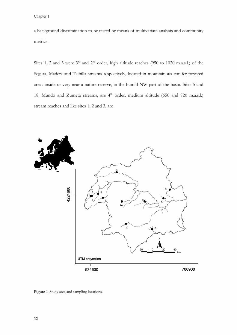
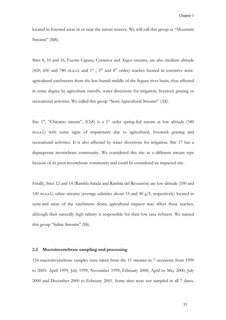
The study sites are located in the Segura River catchment, SE Spain (Figure 1). General
descriptions of the basin area (geology, climate, etc.) can be found elsewhere (Vidal-Abarca
et al., 1992; Mellado et al., 2002). We conducted our study in 11 streams belonging to 4
different typologies: 5 streams in forested mountainous areas, 3 streams located at medium
altitude semi-agricultural areas, 1 spring-fed stream at low altitude, and 2 semiarid naturally
saline streams. These sites were known to harbour different communities from previous
studies (Mellado et al., 2002, Millán et al., 1997; Moreno et al., 1998; Ubero-Pascal et al.,
1998; Vidal-Abarca et al., 1990) and so, this stratified sampling design was supposed to give
Chapter 1
32
a background discrimination to be tested by means of multivariate analysis and community
metrics.
Sites 1, 2 and 3 were 3rd and 2nd order, high altitude reaches (950 to 1020 m.a.s.l.) of the
Segura, Madera and Taibilla streams respectively, located in mountainous conifer-forested
areas inside or very near a nature reserve, in the humid NW part of the basin. Sites 5 and
18, Mundo and Zumeta streams, are 4th order, medium altitude (650 and 720 m.a.s.l.)
stream reaches and like sites 1, 2 and 3, are
Figure 1. Study area and sampling locations.
1
2
3
18
5
16
8
10 14
12
17
1
2
3
18
5
16
8
10 14
12
17
1
2
3
18
5
16
8
10 14
12
17
534600 706900
4224
600
UTM proyection
1
2
3
18
5
16
8
10 14
12
17
1
2
3
18
5
16
8
10 14
12
17
1
2
3
18
5
16
8
10 14
12
17
534600 706900
4224
600
UTM proyection
Chapter 1
33
located in forested areas in or near the nature reserve. We will call this group as “Mountain
Streams” (MS).
Sites 8, 10 and 16, Fuente Caputa, Corneros and Argos streams, are also medium altitude
(420, 650 and 780 m.a.s.l. and 1st , 3rd and 4th order) reaches located in extensive semi-
agricultural catchments from the less humid middle of the Segura river basin, thus affected
in some degree by agriculture runoffs, water diversions for irrigation, livestock grazing or
recreational activities. We called this group “Semi-Agricultural Streams” (AS).
Site 17, “Chicamo stream”, (ChS) is a 1st order spring-fed stream at low altitude (340
m.a.s.l.) with some signs of impairment due to agricultural, livestock grazing and
recreational activities. It is also affected by water diversions for irrigation. Site 17 has a
depauperate invertebrate community. We considered this site as a different stream type
because of its poor invertebrate community and could be considered an impacted site.
Finally, Sites 12 and 14 (Rambla Salada and Rambla del Reventón) are low altitude (100 and
140 m.a.s.l.) saline streams (average salinities about 15 and 40 g/L respectively) located in
semi-arid areas of the catchment. Some agricultural impacts may affect these reaches,
although their naturally high salinity is responsible for their low taxa richness. We named
this group “Saline Streams” (SS).
2.2 Macroinvertebrate sampling and processing 134 macroinvertebrate samples were taken from the 11 streams in 7 occasions from 1999
to 2001: April 1999, July 1999, November 1999, February 2000, April to May 2000, July
2000 and December 2000 to February 2001. Some sites were not sampled in all 7 dates.

Chapter 1
34
One single multi-habitat semiquantitative kick-sample, as described by Zamora-Muñoz and
Alba-Tercedor (1996) was taken in each sampling occasion. In our sampling method,
macroinvertebrates are live-sorted in the field from white trays with the aid of a portable
aspirator trying to collect a representation of the community and getting the maximum
diversity as possible, actively searching for rare taxa. The sampling goes on until no new
taxa (at family level) are found in the field with successive trays. We preserved this field
live-sorted subsample in 70% ethanol.
Another multi-habitat kick-sample was preserved in 1 L plastic jars. This sample was
processed in the laboratory using a fixed count subsampling procedure (approximately 200
individuals when achievable) under a 5X magnification lens. Invertebrates were identified
in the laboratory with the aid of a 6.5-64X Olympus microscope to the lowest taxonomic
level (usually genus) except for some dipterans that were identified to families, subfamilies
or tribes, Hirudinea (identified to family), Hydracarina, Tricladida, Oligochaeta, Nematoda,
Ostracoda, Copepoda and Cladocera. For convenience, we use the term “genus” when
referring to the identification level described above.
2.3 Data análisis 2.3.1 Multivariate analysis
We constructed eight data sets combining the factors we wanted to compare: processing
method (live-sorting –LivS- versus laboratory sorting –LabS-), taxonomic resolution (genus
versus family) and data type (presence-absence versus percentage abundance data). Data
were transformed to percentage abundance due to the semi-quantitative nature of the
sampling method. Relative abundance data were 4th-root transformed as recommended by

Chapter 1
35
horne et al. (1999) for an effective discrimination of sites over a wide range of water
quality.
We carried out a series of multivariate analyses for each data set and compared their results
to investigate the effects of seasonality, sample processing method, taxonomic resolution
and data type on the performance of each multivariate model. Firstly, analysis of
similarities (ANOSIM, Clarke, 1993) was performed on Bray–Curtis similarity distances to
test for differences between stream types and seasons. We used a two-way crossed
ANOSIM with stream type and season as four level factors. Each test in ANOSIM
produces an R-statistic, which contrasts the similarities among samples (our replicates)
within a group (stream types or seasons in our case) with the similarities among samples
between groups. R will take values near 1 when the similarities between samples within
groups are higher than those between samples from different groups, and values near -1 in
the opposite case. Values close to 0 are indicative of no differences among groups. Monte
Carlo permutations number was set at 999. Significant ANOSIM results should be
cautiously interpreted as means can be minimally different with much overlap in values
among sample groups yet still produce statistically significant differences. Nevertheless, we
used comparisons of the R-statistic, which has an absolute interpretation of its value and is
not unduly affected by the number of replicates in each group (Clarke and Gorley, 2001),
to compare models’ ability to differentiate groups. As a general guide, R values can be
categorized into 3 broad groups (Clarke and Gorley, 2001): 1. R > 0.75: indicates that there
are large differences and the treatments/groups are well separated; 2. R > 0.5: indicates
clear differences, but the treatments/groups are ‘overlapping’; 3. R < 0.25: indicates
little/no difference and the treatments/groups are barely separable. When ANOSIM
results were significant, we also calculated ANOSIM pair-wise comparisons among stream
types and/or seasons to distinguish among possibly contrasting effects.

Chapter 1
36
Secondly, we use non-metric multidimensional scaling (MDS, Kruskal and Wish, 1978) to
spatially plot the samples. Non-metric multidimensional scaling maps the samples in
ordination space such that the rank order of the distances among samples on the plot
matches their Bray–Curtis similarities, and samples that share similar assemblage
composition will group together. To measure the effectiveness of two-dimensional MDS
ordination plots in preserving the sample relationships Bray-Curtis similarity ranks, the
stress S value (running 100 iterations) was included in each plot (S<0.20 is considered
acceptable, Clarke and Warwick, 1994). Then, we constructed a 95% Gaussian bivariate
probability ellipse (Altman 1978) around the mountain streams (MS) samples in each of the
MDS plots and calculated the percentage of samples belonging to other stream groups that
fell outside of the MS ellipse as a measure of the discriminatory power of each ordination
model. This procedure is based on the last step of the BEAST (Benthic Assessment of
SedimenT) bioassessment method (Reynoldson et al., 1995, 1997, 2001; King and
Richardson, 2002).
To visualize the congruity among results of the eight analyses, a “second stage” MDS
procedure was performed based on the 8 previously obtained similarity matrices. In this
analysis, Spearman rank correlations (ρ) are calculated between each pair of matrices, being
the resulting correlations matrix the base for a new MDS with the original matrices as
elements of the ordination and the ρ coefficient the new “similarity measure”. The closer
appear two analyses, the more similar their results are.
The PRIMER v5 package (Plymouth Routines in Multivariate Ecological Research, Clarke
and Gorley, 2001) was used to perform all multivariate analyses, while probability ellipses
were constructed using STATISTICA v5.0 software package (Stat Soft Inc, 1995).
Chapter 1
37
Seasonal variation should be manifest primarily at the genus level because representatives
of families are likely to be present throughout the year, so again, one-way ANOSIM tests
between stream types were applied for each of three single-season models using genus
identifications, presence absence and fourth-root transformed relative abundance data and
the Bray-Curtis similarity index for these analyses. Comparison of the R value served again
as a measure of the goodness of fit of the models.
2.3.2 Comparison of community metrics
We applied the Iberian Biomonitoring Working Party (IBMWP, formerly BMWP’) (Alba-
Tercedor and Sánchez-Ortega, 1988; Alba-Tercedor and Pujante, 2000; Alba-Tercedor et
al., 2004) biotic index and its relative IASPT (Iberian Average Score per Taxon) as biotic
integrity indices. The IBMWP index is based on the British BMWP (Armitage et al., 1983)
and it was adapted to the Iberian macroinvertebrate fauna by adding some families and
modifying some scores. The IASPT index is calculated by dividing the IBMWP from a
sample by the number of IBMWP families (only those considered in the index) in this
sample.
As diversity measures and particularly richness metrics are known to have high sensitivity
to sample size (Magurran, 1988; Gotelli and Colwell, 2001; Metzeling and Miller, 2001), we
calculated the expected richness (for a simulated 100 individual sample, ES(100)) for each
sample using rarefaction (Simberloff, 1978). In addition we constructed individual-based
rarefaction curves using Ecosim software (Gotelli and Entsminger, 2001) and calculated
the Abundance-based Coverage Estimate of species richness (ACE, Chao et al., 1993)
using EstimateS software (Colwell, 2000) for both live-sorting (LivS) and laboratory
subsampling (LabS) data sets. Differences in the IBMWP and IASPT biotic indices, family
richness (number of families), genus richness (number of genera), rarefied genus richness,

Chapter 1
38
EPT richness (number of taxa belonging to Ephemeroptera, Plecoptera and Trichoptera)
and rare taxa richness (number of singleton taxa per sample) between different processing
methods, seasons and stream types were assessed by a three-way multivariate analysis of
variance (MANOVA). To test for the influence of macroinvertebrate size on the
performance of the processing methods, we calculated two new richness variables: the
number of taxa with a maximal size of more than ca.10 mm. and of less than ca. 2 mm. We
compared these two variables plus the number of chironomid subfamilies between the two
processing methods by ANOVA.
We inspected metrics for normality using normal-probability residual plots and tested
variance homogeneity using Bartlett’s test (p <0.05). All data met the assumptions of
normal residuals, and all but EPT richness, met the assumptions of homogeneity of
variance (Bartlett’s test, 0.088 < p < 0.95). EPT richness was log(x+5)-transformed and
tested again (Bartlett’s test, p=0.71). When MANOVA showed significant differences,
Scheffe a posteriori tests were used to determine which stream types were significantly
different at the 0.05 probability level. The ANOVA-MANOVA subroutine of the
STATISTICA v5.0 software package (Stat Soft Inc, 1995) was used to run these analyses.
We calculated the expected rarefied richness, ES(100), using the DIVERSE subroutine on
PRIMER v5 (Clarke and Gorley, 2001).
3. Results A total of 38638 organisms was processed, belonging to 23 orders, more than 100 families
and around 275 taxa. Insects comprised 66.6 % of total abundance and 87.6 % of total
number of taxa. Within the insects, the most abundant orders were dipterans (38.4 % of
insect abundance), Ephemeroptera (19.5 %) and Trichoptera (9.7 %). Diptera was the most

Chapter 1
39
diverse order with 60 taxa (22 % of total taxa richness), followed by Coleoptera with 55
taxa (20 %), and Trichoptera with 41 taxa (15 %). Overall, the most abundant taxa were the
amphipod Echinogammarus (with 5875 individuals) followed by the midge subfamily
Orthocladiinae (2836), ostracods (2170), and the mayflies Caenis (1664) and Baetis (1526).
Mean live-sorted sample abundance was 351.2 (Range= 27-1133; SD= 204.7;N=67) while
mean laboratory abundance was 222.3 (Range=159-450; SD=54.89; N=67).
3.1 Multivariate análisis The 2-way ANOSIM results for the season factor were always not significant, with Global
R values near to zero in all analyses, indicating no differences in community structure
between seasons (Table 1). As predicted, there were significant global differences among
stream types in all eight combinations of processing methods, taxonomic levels and data
types considered (Table 1). Pair-wise comparisons among the 4 stream types were always
significant too with lesser values of Global R between the mountain and the semi-
agricultural streams groups (Table 1). Focusing on the effects of the sampling-processing
on the multivariate patterns, we obtained higher values of Global R for the live sorted
(LivS) samples, whatever taxonomic level or data type was considered. Taxonomic
resolution influenced ANOSIM results in both processing methods, increasing the value of
Global R mostly when using presence-absence data. Using the family resolution, we
observed marked increases in Global R when switching from presence-absence data to
relative abundance data, despite this increase being bigger for the laboratory processing
(LabS) data set. However, when considering the genus level, increases in Global R using
relative abundance instead of binary data were almost negligible in both cases. As pointed
out above, pair-wise comparisons were significant in all cases. R values ranged from 0.5 to
0.7 for MS-AS comparisons and were close to 1 in the other cases (Table 1).

Chapter 1
40
Table 1. ANOSIM R and associated probability values p obtained for the different analyses
Notes: LivS=Live-sorting; LabS= Laboratory subsampling; Pres/Abs, presence-absence data; MS, mountain streams; AS, semi-agricultural streams; SS, saline streams; ChS, Chicamo spring.
2-way ANOSIM between Stream Types and Seasons and pair-wise comparisons between stream types
Global ANOSIM ANOSIM Pair-wise comparisons between stream types
Sources of variation Stream Types Seasons MS, AS MS, SS MS, ChS AS, SS AS, ChS SS, ChS
Method Taxonomic level Data type Global
R p
(%) Global
R p
(%) R p (%) R p
(%) R p (%) R p
(%) R p (%) R p
(%)
Pres/Abs 0.719 0.1 0.025 28.1 0.481 0.1 0.917 0.1 0.945 0.1 0.705 0.1 0.723 0.1 1,000 0.1 Family
4th-root 0.764 0.1 0.027 26.0 0.512 0.1 0.954 0.1 0.952 0.1 0.862 0.1 0.743 0.1 1,000 0.1
Pres/Abs 0.789 0.1 -0.008 53.0 0.554 0.1 0.975 0.1 0.953 0.1 0.901 0.1 0.846 0.1 0.984 0.1 LabS
Genus 4th-root 0.792 0.1 -0.002 49.9 0.545 0.1 0.981 0.1 0.928 0.1 0.963 0.1 0.776 0.1 1,000 0.1
Pres/Abs 0.796 0.1 0.061 0.95 0.560 0.1 0.984 0.1 0.992 0.2 0.905 0.1 0.858 0.1 0.981 0.1 Family
4th-root 0.824 0.1 0.057 1.08 0.607 0.1 0.991 0.1 0.986 0.1 0.940 0.1 0.872 0.1 0.984 0.1
Pres/Abs 0.853 0.1 0.037 2.02 0.660 0.1 0.994 0.1 0.984 0.1 0.936 0.1 0.928 0.1 0.984 0.1 LivS
Genus 4th-root 0.856 0.1 0.045 1.93 0.657 0.1 0.996 0.1 0.978 0.1 0.963 0.1 0.934 0.1 0.984 0.1
Chapter 1
41
When testing for the seasonal effect on the ability to discriminate among our stream types, we
obtained comparable results for the three single-season models constructed with the LivS data,
with similar ANOSIM R values than that obtained for the combined models (Table 2). However,
the LabS spring model showed a lower discrimination power than the LabS summer and winter
ones.
MDS plots and the BEAST approach to measure the discriminatory power of the ordinations to
discern among stream types reflected similar trends as ANOSIM tests. Saline streams (SS) and
Chicamo spring (ChS) were the best differentiated clusters, whereas Mountain Streams (MS) and
semi-Agricultural Streams (AS) showed slight overlap, with some AS samples the only ones that
fell into the MS 95% probability ellipses in all cases.
Stress values ranged from 0.14 to 0.16 (Figure 2). The models’ discriminatory powers ranged
from 71.8% to 84.6% for the LabS data and from 76.9 to 92.3% for the LivS data (Figure 2).
Globally, LivS models showed higher discriminatory power values than LabS models (average
increase 5.1%). Considering the same taxonomic level and data nature, increases in discriminatory
power were: 5.1 % for family-binary data, 2.6% for family-relative abundance data, 5.1% for
genus-binary and 7.7% for genus-relative abundance data. Also, the effects of the taxonomic
resolution (overall effect 11.5% increase in discriminatory power) were similar for both
processing methods when considering presence-absence data (a 12.8% increase in discriminatory
power by using genus instead of family level) but different when relative-abundance transformed
data were used. For the LabS data, the increase in discriminatory power was 7.7% while for the
LivS data it was 12.8%. The nature of the data (binary versus transformed relative abundance)
had less influence on the discriminatory power of the ordinations than taxonomic resolution

Chapter 1
42
(average increase 2.6%). A 5% increase in discriminatory power was achieved for the LabS data at
the family level, while no effect was detected at the genus level. For the field-processed data, a
2.6% increase was detected at both taxonomic levels. To sketch out the influence of the data
transformation, we performed the same 2-way ANOSIM tests for untransformed relative
abundance data, ranging the R values from 0.488 to 0.593, around 25% lower values than R for
4th-root transformed or binary data.
The 2nd-stage MDS procedure showed two clear patterns (Figure 3): In a first axis (horizontal),
the analyses were clearly separated by the processing method, being the LivS analyses in the left
side of the MDS plot and the LabS ones in the right side. The second axis (vertical) separated the
analyses mainly by the taxonomic resolution used, with the genus level analyses arranged in the
upper part of the plot. Secondarily, the nature of the data was also discriminated in this vertical
axis, with transformed relative abundance data approaches located above presence-absence ones,
a trend much more marked for family than for genus taxonomic level, for which the nature of the
data had very little influence.
Table 2. Between stream-types ANOSIM R and associated probability values p obtained for the three single-season and the combined models.
Comparison of three single-season models for ANOSIM “between stream types”
Seasonal ANOSIM: Spring Summer Winter All Seasons
Method Data type Global R
p (%)
Global R
p (%)
Global R
p (%)
Global R
p (%)
Pres/Abs 0.713 0.1 0.845 0.1 0.807 0.1 0.789 0.1 LabS
4th-root 0.724 0.1 0.836 0.1 0.801 0.1 0.792 0.1
Pres/Abs 0.833 0.1 0.865 0.1 0.867 0.1 0.853 0.1 LivS
4th-root 0.863 0.1 0.879 0.1 0.846 0.1 0.856 0.1 Notes: LivS=Live-sorting; LabS= Laboratory subsampling. Pres/Abs, presence-absence data. (Genus level data were used)

Chapter 1
43
Figure 2. Non-metric multiple dimensional scaling (MDS) plots for each of the eight factors combinations. 95% probability ellipses are plotted around the mountain streams (MS) group. Stress value (S) is included in each ordination and the percentage accuracy or discriminatory power between MS and the other stream groups is written near the ellipses.
Relative abundancePresence-absence Presence-absence Relative abundance
S=0.14
Family level Genus level
LabS
dat
aLi
vS d
ata
Mountain streams (MS)Semi-agricultural streams (AS)Saline streams (SS)Chicamo spring (ChS)
S=0.16
71.8
S=0.16
76.9
S=0.15
84.6
S=0.15
84.6
S=0.1676.9 S=0.14
79.5
92.3
S=0.1489.7

Chapter 1
44
Figure 3. 2nd-Stage non-metric Multiple Dimensional Scaling (MDS) plot showing the relative positions of the different analyses evaluated. (LivS=live-sorting; LabS= laboratory subsampling; G=Genus level; F=Family level; PA=Presence-absence data; RA= 4th root-transformed Relative Abundance data)
3.2 Comparison of community metrics MANOVA did not detect significant differences in any biological variable among seasons (Table
3). In contrast and as we expected, biotic variables were significantly different among stream
groups (Tables 3 and 4). All metrics with the exception of the IASPT index showed significant
differences between processing methods, with higher values obtained for the LivS method
(Figure 4). We found also a significant interaction between stream type and processing method in
family richness and genus richness, due to higher increases in richness from LabS to LivS in the
more diverse communities (MS and AS streams) than in poorer ones (SS and ChS), where the
LabS effort was enough to reach similar taxa numbers with LivS (Figure 5).
Rarefaction curves were different between methods, with LivS expected richness values always
higher than LabS ones. The ACE estimate of asymptotic genus richness was also higher for the
LivS data set (267 versus 227, Figure 6).We also found significantly higher number of taxa of
both large (F=10.09; p=0.00197) and small (F=26.41; p=0.000001) organisms in LivS samples
(Figure 4). The number of Chironomidae subfamilies was not different among methods (F=0.06;
p=0.80).
Stress: 0,01
Liv-S-F-PA
Liv-S-F-RA
Liv-S-G-PA Liv-S-G-RA
LabS-F-PA
LabS-F-RA
LabS-G-PA
LabS-G-RA
Stress: 0,01
Liv-S-F-PA
Liv-S-F-RA
Liv-S-G-PA Liv-S-G-RA
LabS-F-PA
LabS-F-RA
LabS-G-PA
LabS-G-RA

Chapter 1
45
Table 3. Multivariate analysis of variance (MANOVA) on community metrics. Factors and variables to which significant effects were found (p<0.05) are in bold.
MANOVA summary of all effects Factors Wilks' Lambda Rao's R df 1 df 2 p Stream type (ST) 0.05125 23.86 21 276 0.0000 Season (SE) 0.74937 1.39 21 276 0.1216 Processing method (PM) 0.81328 3.15 7 96 0.0049
ST x SE 0.63989 0.72 63 546 0.9502 ST x PM 0.47622 3.88 21 276 0.0000 SE x PM 0.79877 1.07 21 276 0.3798 ST x SE x PM 0.63066 0.74 63 546 0.9311 Main effect: stream type Main effect: season MS Effect MS Error F (df 3,102) p MS Effect MS Error F(df 3,102) p Family richness 2484.546 35.429 70.13 0.0000 Family richness 24.556 35.429 0.69 0.5583 IBMWP index 98271.62 1277.962 76.90 0.0000 IBMWP index 651.696 1277.962 0.51 0.6763 IASPT index 20.88038 0.251 83.10 0.0000 IASPT index 0.342 0.251 1.36 0.2586 Genus richness 4686.726 81.148 57.76 0.0000 Genus richness 69.339 81.148 0.85 0.4674 EPT richness 5.194952 0.052 99.44 0.0000 EPT richness 0.056 0.052 1.06 0.3682 Rare richness 828.7542 15.015 55.20 0.0000 Rare richness 5.333 15.015 0.36 0.7855 Estimated richness ES(100) 2085.458 34.816 59.90 0.0000 Estimated richness
ES(100) 91.103 34.816 2.62 0.0551
Main effect: processing method Main effect: Interaction ST x PM MS Effect MS Error F (df 1,102) p MS Effect MS Error F(df 3,102) p Family richness 624.594 35.429 17.63 0.0001 Family richness 107.582 35.429 3.04 0.0325 IBMWP index 10346.185 1277.962 8.10 0.0054 IBMWP index 2652.325 1277.962 2.08 0.1081 IASPT index 2.0262E-05 0.251 0.00 0.9929 IASPT index 0.155 0.251 0.61 0.6068 Genus richness 1305.895 81.148 16.10 0.0001 Genus richness 279.160 81.148 3.44 0.0196 EPT richness 0.329 0.052 6.29 0.0137 EPT richness 0.133 0.052 2.54 0.0605 Rare richness 79.115 15.015 5.27 0.0238 Rare richness 16.519 15.015 1.10 0.3527 Estimated richness ES(100) 289.054 34.816 8.30 0.0048 Estimated richness
ES(100) 72.236 34.816 2.07 0.1082

Chapter 1
46
Table 4. Means and standard deviations (SD) of community metrics within stream types. Means with different superscripts are significantly different at p<0.05 (Scheffe tests).
Variable:
FAM_R
GEN_R
ES(100)
EPT_R
TYPE Mean SD Mean SD Mean SD Mean SD
MS 32.20a 7.78 42.75a 11.88 30.23a 7.40 11.89a 4.25
AS 29.11b 7.62 38.31b 11.71 26.23b 7.32 8.17b 3.15
SS 12.92c 4.25 17.12c 6.65 13.31c 5.20 1.54c 1.17
ChS 14.82c 4.19 16.88c 5.28 13.76c 4.49 3.29d 1.31
Variable:
RARE_R
IBMWP
IASPT
TYPE Mean SD Mean SD Mean SD
MS 15.09a 4.53 171.39a 47.07 5.53a 0.59
AS 12.51b 4.43 121.94b 35.08 4.43b 0.35
SS 4.00c 1.85 47.00c 18.96 3.66c 0.40
ChS 5.24c 2.05 60.53c 16.90 4.51b 0.46 Note: MS, mountain streams; AS, semi-agricultural streams; SS, saline streams; ChS, Chicamo spring.
FAM_R, number of families; GEN_R, number of gena; EPT_R, number of Ephemeroptera, Plecoptera and Trichoptera taxa;
RARE_R, number of singleton taxa.
4. Discussion Among the most important technical issues for RBPs using macroinvertebrates are:
seasonality, sampling methodology, subsampling and sorting and taxonomic identification
level (Barbour et al., 1999). If we achieve a time-cost effectiveness by reducing effort in
each one of these issues, we are then improving the RBPs applicability, which is the
ultimate sense of such rapid approaches.
4.1 Seasonality We did not find any pattern of seasonal trends that could have obscured the grouping of
samples from the same stream typology. Seasonal samples from each of the stream types
tended to be more similar to themselves than to any of the other stream types. Although

Chapter 1
47
Figure 4. Comparison of community variables between laboratory subsamples (LabS, white bars) and live-sorted samples (LivS, black bars). All variables but IASPT showed significant differences at p<0.05 (MANOVA).
Figure 5.Mean family richness (black circles) and genus-richness (open squares) variations with processing method in each stream type (MS= mountain streams; AS= semi-agricultural streams; SS= saline streams and ChS= Chicamo spring). ANOVA stream type x processing method interaction was significant for family richness (F=3.04, p<0.05) and genus richness (F=3.44, p<0.05).
MS
5
10
15
20
25
30
35
40
45
50
55AS SS ChS
STREAM TYPE
LabS LabS LabS LabSLiv-S Liv-SLiv-SLiv-S
PROCESSING METHOD
MS
5
10
15
20
25
30
35
40
45
50
55AS SS ChS
STREAM TYPE
LabS LabS LabS LabSLiv-S Liv-SLiv-SLiv-S
PROCESSING METHOD
Fam
ily le
vel N
o. o
f tax
a
0
10
20
30
40
50
IBM
WP
bio
tic in
dex
0
50
100
150
200
250
IAS
PT
biot
ic in
dex
0
1
2
3
4
5
6
7G
enus
leve
l No.
of t
axa
0
10
20
30
40
50
60
No.
of E
PT ta
xa
0
2
4
6
8
10
12
14
16
No.
of R
ARE
taxa
0
5
10
15
20
Rar
efie
d E
S (1
00)
0
10
20
30
40
No.
of l
arge
taxa
0
2
4
6
8
10
No.
of s
mal
l tax
a
0
2
4
6
8
10
12
14
16
Fam
ily le
vel N
o. o
f tax
a
0
10
20
30
40
50
IBM
WP
bio
tic in
dex
0
50
100
150
200
250
IAS
PT
biot
ic in
dex
0
1
2
3
4
5
6
7G
enus
leve
l No.
of t
axa
0
10
20
30
40
50
60
No.
of E
PT ta
xa
0
2
4
6
8
10
12
14
16
No.
of R
AR
E ta
xa
0
5
10
15
20
Rar
efie
d E
S (1
00)
0
10
20
30
40
No.
of l
arge
taxa
0
2
4
6
8
10
No.
of s
mal
l tax
a
0
2
4
6
8
10
12
14
16

Chapter 1
48
Figure 6. Individuals based rarefaction curves for laboratory subsampling (LabS) and live-sorting (LivS) data sets. Abundance based Coverage Estimate of richness (ACE) for each data set is included.
we couldn’t test for seasonal differences within sites due to the lack of replication,
additional ANOSIM tests within stream types (MS and AS, the most represented groups)
did not reflect any seasonal pattern (these results have been omitted for brevity). In
addition, when we compared 3 single-season models (spring, summer and winter) in
differentiating stream groups, we did not observe strong differences among them when
considering the field processed data. However, when looking at fixed-count laboratory
sorted samples, some differences between single-season multivariate models appeared, with
the spring model performing worst relative to summer and winter ones in detecting
between-group differences.
MANOVA did not show seasonal differences for any of the variables considered. These
results were consistent among processing methods and stream types. None of the
interactions with the season factor were significant, supporting the results obtained in
multivariate analyses and indicating the seasonal stability of the benthic macroinvertebrate
0
50
100
150
200
250
0 5000 10000 15000 20000 25000
Individuals
Rar
efie
d ric
hnes
s
LivS data
LabS data
ACE=227ACE=227
ACE=267
0
50
100
150
200
250
0 5000 10000 15000 20000 25000
Individuals
Rar
efie
d ric
hnes
s
LivS data
LabS data
ACE=227ACE=227
ACE=267

Chapter 1
49
communities studied. These results are indicative of a temporal persistence in community
patterns (at least at a reach spatial scale and a 2 years temporal scale) that would be required
for bioassessment programs based on pattern detection (Bunn and Davies, 2000).
Moreover, our results suggest the suitability of a single season approach for biomonitoring
purposes in the study area, circumventing the need for seasonal corrections of biotic
integrity metrics (Lenat, 1993; Whiles et al., 2000) or the use of single-season or combined
seasons models (Reece et al., 2001) needed in other regions.
4.2 Processing method Some RBPs involve a live-sorting methodology in which live organisms are picked from a
tray just after sampling (Lenat, 1988; Chessman, 1995; Tiller and Metzeling, 1998;
Metzeling and Miller, 2001). Some 23% of the monitoring programs in US used a live-
sorting methodology, 75% of which focused on maximizing faunal richness (Carter and
Resh, 2001). Although it had been argued that laboratory processing is desirable to
standardize conditions and ensure randomness, the live-sorting is more time-cost efficient
because picking up live animals is easier because movements help to find them. It is also
more effective in terms of getting higher diversities because small and cryptic creatures can
be seen better while moving. Moreover, the active searching for rare species increasing
richness values which is critical for bioassessment purposes (Cao et al., 1998; 2001).
On the other hand, collecting animals separately while alive avoids the undesirable high
amounts of organic detritus and sediment that occur when whole samples are taken, which
means a better efficiency in terms of time in subsequent laboratory sorting. Moreover, the
sampled area can be much wider and again the number of species collected. Additionally,
using a portable aspirator helps to capture organisms too small and/or fragile to be picked

Chapter 1
50
up with forceps, as ostracods, small snails or early instars insects, as well as to capture
highly mobile animals as baetid mayflies or dytiscid beetles, circumventing the bias argued
by Carter and Resh (2001) on rapidly moving taxa when sorting live material. The field live-
sorting substantially minimizes the amount of preservative used, avoids the unintentional
capture of organisms belonging to threatened species, and minimizes the possible sampling
disturbance on communities, especially in small habitats. Finally, it offers the possibility of
obtaining immediate field data sets (see BioRecon protocols in Barbour et al., 1999;
Chessman, 1995) with moderately trained technicians (family level identification) that can
be crucial for rapid bioassessment application.
Humphrey and Thurtell (1997) and Metzeling (2001) recommend a field sorting of at least
200 individuals for up to 60 minutes under the Monitoring River Health Initiative in
Australia. Canada’s EMAN protocols for measuring biodiversity suggest a 15-min sorting
period or a target of 300 individuals (Rosenberg et al., 1997). We collected a mean number
of organisms of approximately 350 organisms, and the time spent sorting a sample was
around 40 minutes. We have tested the applicability and performance of a live-sorting field
methodology and the results obtained are better than those achieved with a fixed count
subsample of ca. 200 in the laboratory. ANOSIM significantly differentiated the stream
types for both processing methods, however, values of the R statistic were always higher
for LivS than for LabS analyses, and discriminatory power, as estimated by the BEAST
ellipses method, was also greater using LivS data, with an average increase of 5.1%.
Although it is not a marked improvement, it is an additional advantage of the use of the
live-sorting methodology.
Differences in community metrics also illustrated the better performance of the field
processing methodology. All metrics but the IASPT index showed significant increases

Chapter 1
51
when applying the live-sorting methodology (Figure 4). The IASPT index is less affected by
taxonomic richness than IBMWP, and thus it was not influenced by the processing
method. The fact that not only the observed richness but also the rarefied expected
richness showed a significant increase (Figure 4), demonstrate that the higher effectiveness
of the live-sorting is affecting richness values, instead of being simply a sample size
(number of organisms collected per sample) effect. This is illustrated by the rarefaction
curves for both processing methods and the ACE expected richness values (Figure 6).
Furthermore, the higher values found for the number of rare species (Figure 4) also
suggested a better performance of the live-sorting procedure in maximizing biodiversity.
The significant interaction found between stream type and processing method is
interpreted as a higher reliance on the methodology in taxonomic richer environments. The
IBMWP index is interpreted categorically in the following manner: scores of >100 (class I)
are indicative of clean water, 61–100 (class II) of mild pollution, 36-60 (class III) polluted
waters, 16-36 (class IV) very polluted waters and <16 (class V) strongly polluted waters.
Considering IBMWP quality classes, 36% of the sites experienced a decrease in quality
from LivS to LabS data showing that not only absolute values are affected by the sampling-
processing methodology, but also the quality classes. This reinforces the idea that the
correct application of this index must incorporate its original protocol.
Humphrey et al., (2000) found that live-sorting methods used by some water agencies of
Australia were less successful in terms of number of taxa recovered than laboratory sorting
ones. We have found an opposite trend, probably due to the nature of our sampling
procedure: as we argued above, the sampled area for live-sorting, although not estimated,
was probably wider than the area sampled to take the preserved sample. Another likely
reason explaining the higher taxa richness in live-sorted samples is the use of the aspirator,
much more efficient than forceps or wide mouthed pipettes in our opinion. Moreover, we

Chapter 1
52
did not find any bias concerning the size of the organisms, having captured significantly
more both larger (>10 mm) and smaller (<2 mm) organisms in live-sorted samples. The
number of Chironomidae subfamilies neither was different among methods.
4.3 Taxonomic resolution and data type Comparative studies of assemblages require decisions about the level of taxonomic
resolution to which organisms are identified, and the biological attributes to be measured –
presence-absence or abundance (Lasiak, 2003). If a comparative pattern persists at a lower
taxonomic resolution (i.e. family level), then it is an advantage to use that lower level in
terms of time and cost required to obtain meaningful information from a sampling
program (Metzeling and Miller, 2001). Several analyses of benthic macroinvertebrate
communities have shown little change in the multivariate description of community
changes at different taxonomic levels (e.g. Furse et al., 1984, Bowman and Bailey, 1998). In
our case, while the use of less precise taxonomic levels did not affect the significance of
ANOSIM tests, the use of genus identifications was the main factor increasing ANOSIM R
values and also the discriminatory power of the MDS-BEAST models. As we pointed out
before, discriminatory power between MS and SS or ChS samples was in all cases 100%,
which we can interpret as a separation of communities due to degradation or to extreme
differential environmental features (ej. salinity). However, differences in model
performance arose when comparing the ability to discriminate between moderately
impacted semi-agricultural streams and mountain streams, both representing taxonomically
richer ecosystems. In this case, the use of genus level resolution increased the accuracy by
11.5%, more than double that of processing method (5.1%) and four times more than data
type (2.6%) on average. Bowman and Bailey (1998) also found that community descriptions
based on genus-level identifications were less similar than descriptions based on family-

Chapter 1
53
level identifications when the overall fauna was more diverse. Bailey et al., (2001) suggested
a family-level broad bioassessment followed by a genus level identification if more precise
information is needed. Our results would support this approach. On the other hand, the
extent to which taxonomic aggregation affects multivariate analyses will also depend on the
species distribution amongst higher taxa (Somerfield and Clarke, 1995), so generalizations
should not be done about the correct resolution level to use before testing its effect on
target communities.
Some studies have shown that spatial patterns of macroinvertebrate communities evident
in quantitative data are generally preserved in binary data (Furse et al.,1984; Wright et
al.,1995; Thorne et al., 1999). Our study supports these results, with little increases in
ordination accuracy at the family level when transformed relative abundance was used and
no influence at the genus level. A possible explanation is that when genus level is used,
abundances are more equally distributed among taxa, with more low abundance or rare
taxa. Thus, a relative abundance matrix is more similar to a binary one. In contrast, when
aggregating genus into families, percentages of abundance will change because of the
differential distribution of genera within families so differences with the presence-absence
data matrix will increase too. Thorne et al. (1999) recommended a severe down-weighting
of abundant taxa when comparisons are being made between relatively unpolluted sites
with high richness. Binary data and fourth root-transformation represent such severe
down-weighting of abundant taxa. 2-way ANOSIM tests for untransformed data resulted
in R values ranging from 0.488 to 0.593, around 25% lower values than R for 4th-root
transformed or binary data, so our results strongly support adopting this data
transformation. Nevertheless, the small increase in performance associated with the high
effort of counting individuals lead us recommend the use of binary data for bioassessment
purposes. On the other hand, family and genus numbers of taxa showed similar trends

Chapter 1
54
between stream types, seasons and processing methods, probably due to the great number
of families containing low numbers of genus in our data set (86 families with 4 or less
genus versus only 16 with 5 or more).
Our study has four important implications: 1) A single season sample provides enough
information to detect patterns of change in macroinvertebrate communities in our region,
2) The live-sorting procedure performed better than the laboratory fixed-count
subsampling and did not show size-dependent bias, 3) Family level identification provides
comparable results to the genus level at a broader environmental scale, while genus
identification performed better at detecting subtle differences within communities, and 4)
Presence-absence data can explain the majority of variation in community structure.
5. References Alba-Tercedor, J. 2000. ‘BMWP’, un adattamento spagnolo del British Biological Monitoring Working Party (BMWP) Score System. Biologia Ambientale 17 (2), 65-67. Alba-Tercedor, J. and Pujante, A. 2000. Running-water biomonitoring in Spain: opportunities for a predictive approach. in: J.F. Wright, D.W. Sutcliffe and M.K. Furse (eds). Assessing the biological quality of freshwater, RIVPACS and other techniques. Freshwater Biological Association, Ambleside, Cumbria, UK, pp. 207-216. Alba-Tercedor, J. and Sánchez-Ortega, A. 1988. Un método rápido y simple para evaluar la calidad biológica de las aguas corrientes basado en el de Hellawell (1978). Limnetica 4, 51-56. Alba-Tercedor, J., Jáimez-Cuéllar, P., Álvarez, M., Avilés, J., Bonada, N., Casas, J., Mellado, A., Ortega, M., Pardo, I., Prat, N., Rieradevall, M., Robles, S., Sáinz-Cantero, C.E., Sánchez-Ortega, A., Suárez, M.L., Toro, M., Vidal-Abarca, M.R., Vivas, S. and Zamora-Muñoz, C. 2004. Caracterización del estado ecológico de ríos mediterráneos ibéricos mediante el índice IBMWP (antes BMWP’). Limnetica 21, 2002 (3-4), 175-185 Altman, D.G. 1978. Plotting probability ellipses. Applied Statistics 27, 347–349.

Chapter 1
55
Armitage, P.B., Moss, D., Wright, J.F. and Furse, M.T. 1983. The performance of a new biological water quality score system based on macroinvertebrates over a wide range of unpolluted running-water. Water Research 17 (3), 333-347. Bailey, R.C., Norris, R.H. and Reynoldson, T.B. 2001. Taxonomic resolution of benthic macroinvertebrate communities in bioassessments. Journal of the North American Benthological Society 20, 280–286. Barbour, M.T. and Gerritsen, J. 1996. Subsampling of benthic samples: a defense of the fixed-count method. Journal of the North American Benthological Society 15, 386–391. Barbour, M.T., Gerritsen, J., Snyder, B.D., and Stribling, J.B. 1999. Rapid Bioassessment Protocols for Use in Streams and Wadeable Rivers: Periphyton, Benthic Macroinvertebrates and Fish. Second Edition EPA 841-B-99-002’, U.S. Environmental Protection Agency; Office of Water; Washington DC. Boulton, A.J. and Lake, P.S. 1992. The ecology of two intermittent streams in Victoria, Australia. III. Temporal changes in faunal composition. Freshwater Biology 27, 123–138. Bournaud, M., Cellot, B., Richoux, P. and Berrahou, A. 1996. Macroinvertebrate community structure and environmental characteristics along a large river: congruity of patterns for identification to species or family. Journal of the North American Benthological Society 15, 232–253. Bowman, M.F. and Bailey, R.C. 1998. Does taxonomic resolution affect the multivariate description of the structure of freshwater benthic macroinvertebrate communities?. Canadian Journal of Fisheries and Aquatic Sciences 54, 1802–1807. Brunke, M., Hoffmann, A. and Puscha, M. 2001. Use of mesohabitat-specific relationships between flow velocity and river discharge to assess invertebrate minimum flow requirements. Regulated Rivers: Research and Management 17, 667–676. Bunn, S.E. and Davies, P.M. 2000. Biological processes in running waters and their implications for the assessment of ecological integrity. Hydrobiologia 422, 61-70. Cao, Y., Williams, D.D. and Williams, N.E. 1998. How important are rare species in aquatic community ecology and bioassessment?. Limnology and Oceanography 43, 1403–1409. Cao, Y., Larsen, D.P. and Thorne, R.S.J. 2001. Rare species in multivariate analysis for bioassessment: some considerations. Journal of the North American Benthological Society 20, 144–153.

Chapter 1
56
Carter, J.L., and Resh, V.H. 2001. After site selection and before data analysis: sampling, sorting, and laboratory procedures used in stream benthic macroinvertebrate monitoring programs by USA state agencies. Journal of the North American Benthological Society 20, 658–682. Chao, A., Ma, M.C. and Yang, M.C.K. 1993. Stopping rules and estimation for recapture debugging with unequal failure rates. Biometrika 80, 193-201. Chessman, B.C. 1995. Rapid assessment of rivers using macroinvertebrates: a procedure based on habitat-specific sampling, family-level identification and a biotic index. Australian Journal of Ecology 20, 122–129. Chessman, B.C. 1999. Predicting the macroinvertebrate faunas of rivers by multiple regression of biological and environmental differences. Freshwater Biology 41, 747-757 Clarke, K.R. 1993. Non-parametric multivariate analysis of changes in community structure. Australian Journal of Ecology 18, 117-143. Clarke, K.R. and Gorley, R.N. 2001. PRIMER v5: User Manual/Tutorial. PRIMER-E, Plymouth. Clarke, K.R., and Warwick, R.M. 1994. Changes in marine communities: an approach to statistical analysis and interpretation. Plymouth Marine Laboratory, Plymouth. Colwell, R.K. 2000. EstimateS: Statistical Estimation of Species Richness and Shared Species from Samples (Software and User's Guide), Version 6. (http://viceroy.eeb.uconn.edu/estimates) Courtemanch, D.L. 1996. Commentary on the subsampling procedures used for rapid bioassessments. Journal of the North American Benthological Society 15, 381–385. Death, R.G. 1995. Spatial patterns in benthic invertebrate community structure: products of habitat stability or are they habitat specific? Freshwater Biology 33, 455-467. Doberstein, C.P., Karr, J.R. and Conquest, L.L. 2000. The effect of fixed-count subsampling on macroinvertebrate biomonitoring in small streams. Freshwater Biology 44, 355–371. European Commission. 2000. Directive of the European Parliament and of the Council 2000/60/EC establishing a framework for community action in the field of water policy, European Commission PE-CONS 3639/1/00 REV 1. European Commission, Luxembourg.

Chapter 1
57
Feminella, J.W. 1996. Comparison of benthic macroinvertebrate assemblages in small streams along a gradient of flow permanence. Journal of the North American Benthological Society 15, 651–669. Fisher, S.G., Gray, L.J., Grimm, N.B. and Bush, D.E. 1982. Temporal succession in a desert stream ecosystem following flash flooding. Ecological Monographs 52, 93–110. Furse, M.T., Moss, D., Wright, J.F. and Armitage, P.D. 1984. The influence of seasonal and taxonomic factors on the ordination and classification of running-water sites in Great Britain and on the prediction of their macroinvertebrate communities. Freshwater Biology 14, 257–280. Giller, P.S. and Malmqvist, B. 1998. The Biology of Streams and Rivers. Oxford University Press, Oxford. Gotelli, N.J. and Colwell, R.K. 2001. Quantifying biodiversity: procedures and pitfalls in the measurement and comparison of species richness. Ecology Letters 4, 379-391. Gotelli, N.J. and Entsminger, G.L. 2001. Ecosim: Null Models Software for Ecology. Version 6.0. Acquired Intelligence Inc. and Kesey-Bear. http://homepages.together.net/gentsmin/ecosim.htm Guerold, F. 2000. Influence of taxonomic determination level on several community indices. Water Research 34 (2), 487-492. Hawkins, C.P. and Sedell, J.R. 1981. Longitudinal and seasonal changes in functional organization of macroinvertebrate communities in four Oregon streams. Ecology 62, 387-397. Humphrey, C.L. and Thurtell, L. 1997. External QA/QC of MRHI agency subsampling and sorting procedures: Results for 1995 and 1996. Land and Water Resources Research and Development Corporation, Camberra. Humphrey, C.L., Storey, A.W., and Thurtell, L. 2000. AUSRIVAS: operator sample processing errors and temporal variability – implications for model sensitivity. in, J.F. Wright, D.W. Sutcliffe and M.T Furse (eds). Assessing the biological quality of fresh waters. RIVPACS and other techniques. Freshwater Biological Association, Ambleside, Cumbria, UK. pp 143-163. King, R.S. and Richardson, C.J. 2002. Evaluating subsampling approaches and macroinvertebrate taxonomic resolution for wetland bioassessment. Journal of the North American Benthological Society 21(1), 150–171.
Chapter 1
58
Kruskal, J.B. and Wish, M. 1978. Multidimensional scaling. Sage, Beverley Hills. Lasiak, T. 2003. Influence of taxonomic resolution, biological attributes and data transformations on multivariate comparisons of rocky macrofaunal assemblages. Marine Ecology Progress Series 250, 29–34. Lenat, D.R. 1988. Water quality assessment of streams using a semi-quantitative collection method for benthic macroinvertebrates. Journal of the North American Benthological Society 7, 222–233. Lenat, D.R. 1993. A biotic index for the southeastern United States: derivation and list of tolerance values, with criteria for assigning water-quality ratings. Journal of the North American Benthological Society 12, 279 –290. Lenat, D.R. and Resh, V.H. 2001. Taxonomy and stream ecology —The benefits of genus- and species-level identifications. Journal of the North American Benthological Society 20, 287–298. Linke, S., Bailey, R.C. and Schwindt, J. 1999. Temporal variability of stream bioassessments using benthic macroinvertebrates. Freshwater Biology 42, 575-584. Magurran, A.E. 1988. Ecological diversity and its measurement. Princeton University Press, Princeton. Mellado, A., Suárez, M.L., Moreno, J.L. and Vidal-Abarca, M.R. 2002. Aquatic macroinvertebrate biodiversity in the Segura River basin (SE Spain). Verh. Internat. Verein. Limnol. 28, 1157-1162. Millán, A., Velasco, J., Vidal-Abarca, M.R., Suárez, M.L. and Ramírez Díaz, L. 1997. Distribución espacial de los Adefaga acuáticos (Coleoptera) en la cuenca del Río Segura (SE de la Península Ibérica). Limnetica 12 (2), 13-29. Metzeling, L. 2001. Australia-Wide Assessment of River Health: Victoria Bioassessment Report (VIC Final Report). Monitoring River Heath Initiative Technical Report no 4’, Commonwealth of Australia and VIC Environment Protection Authority, Australia. Metzeling, L. and Miller, J. 2001. Evaluation of the sample size used for the rapid bioassessment of rivers using macroinvertebrates. Hydrobiologia 444, 159–170. Moreno, J.L., Millán, A., Suárez, M.L., Vidal-Abarca, M.R. and Velasco, J. 1997. Aquatic Coleoptera and Heteroptera assemblages in waterbodies from ephemeral coastal streams (“ramblas”) of south-eastern Spain. Archiv für Hydrobiologie 141 (1), 93-107.

Chapter 1
59
Murphy, P.M. 1978. The temporal variability in biotic indices. Environmental Pollution 17, 227-236. Murphy, J.F. and Giller, P.S. 2000. Seasonal dynamics of macroinvertebrate assemblages in the benthos and associated with detritus packs in two low-order streams with different riparian vegetation. Freshwater Biology 43, 617-631. Parsons, M., and Norris, R.H. 1996. The effect of habitat-specific sampling on biological assessment of water quality using a predictive model. Freshwater Biology 36, 419–34. Plafkin, J.L., Barbour, M.T., Porter, K.D., Gross, S.K. and Hughes, R.M. 1989. Rapid bioassessment protocols for use in streams and rivers: benthic macroinvertebrates and fish. Report No. EPA/440/4-89/001. US Environmental Protection Agency, Office of Water Regulations and Standards, US. Prat, N. 2002. El Proyecto Guadalmed. Limnetica 21 (3-4), 1-3. Reece, P.F., Reynoldson, T.B., Richardson, J.S. and Rosenberg, D.M. 2001. Implications of seasonal variation for biomonitoring with predictive models in the Fraser River catchment, British Columbia. Canadian Journal of Fisheries and Aquatic Sciences 58, 1411–1418. Resh, V.H. and Jackson, J.K. 1993. Rapid assessment approaches to biomonitoring using benthic macroinvertebrates. in: D. M. Rosenberg and V. H. Resh (eds). Freshwater Biomonitoring and Benthic Macroinvertebrates, Chapman and Hall, New York. pp. 195–233. Resh, V.H., Norris, R.H. and Barbour, M.T. 1995. Design and implementation of rapid assessment approaches for water resource monitoring using benthic macroinvertebrates. Australian Journal of Ecology 20, 108–121. Reynoldson, T.B., Bailey, R.C., Day, K.E. and Norris, R.H. 1995. Biological guidelines for freshwater sediment based on BEnthic Assessment of SedimenT (the BEAST) using a multivariate approach for predicting biological state. Australian Journal of Ecology 20, 198-219. Reynoldson, T.B., Norris, R.H., Resh, V.H., Day, K.E., and Rosenberg, D.M. 1997. The reference condition: a comparison of multimetric and multivariate approaches to assess water-quality impairment using benthic macroinvertebrates. Journal of the North American Benthological Society 16, 833–852. Reynoldson, T.B., Rosenberg, D.M. and Resh, V.H. 2001. Comparison of models predicting invertebrate assemblages for biomonitoring in the Fraser River catchment, British Columbia. Canadian Journal of Fisheries and Aquatic Sciences 58, 1395-1410.

Chapter 1
60
Rosenberg, D.M., Davies, I.J., Cobb, D.G. and Wiens, A.P. 1997. Ecological Monitoring and Assessment Network (EMAN) protocols for measuring biodiversity: benthic macroinvertebrates in fresh waters. prepared for EMAN Office, Environment Canada, Burlington (EMAN website: www.cciw.ca./eman-temp/intro.html) Simberloff, D. 1978. Use of rarefaction and related methods in ecology. in: K.L. Dickson, J. Jr. Cairns and R.J. Livingston (eds). Biological Data in Water Pollution Assessment: Quantitative and Statistical Analyses. American Society for Testing and Materials, Philadelphia, U.S.A. pp. 150-165. Somerfield, P.J. and Clarke, K.R. 1995. Taxonomic levels, in marine community studies, revisited. Marine Ecology Progress Series 127, 113–119 Somers, K.M., Reid, R.A. and David, S.M. 1998. Rapid biological assessments: how many animals are enough?. Journal of the North American Benthological Society 17, 348–358. StatSoft, Inc.: 1995. STATISTICA for Windows, Tulsa, OK, USA. Thorne, R.J., Williams, W.P. and Cao, Y. 1999. The influence of data transformations on biological monitoring studies using macroinvertebrates. Water Research 33 (2), 343-350. Tiller, D. and Metzeling, L. 1998. Rapid Bioassessment Methods Used by the Environment Protection Authority in Victoria, Publication No. 604. Environment Protection Authority (EPA), Victoria, Australia. Ubero-Pascal, N.A., Puig, M.A. and Soler, A.G. 1998. Los Efemerópteros de la cuenca del río Segura (S.E. de España): 1. Estudio faunístico. (Insecta: Ephemeroptera). Boletín de la Asociación Española de Entomología 22 (1-2), 151-170 Vidal-Abarca, M.R., Montes, C., Suárez, M.L. and Ramirez Diaz, L. 1990. Sectorización ecológica de cuencas fluviales: aplicación a la cuenca del río Segura (SE España). Anales de Geografía de la Universidad Complutense 10, 149–182. Vidal-Abarca, M.R., Montes, C., Suárez, M.L. and Ramirez Diaz, L. 1992. An approach to the ecological characterization of arid and semiarid basins. Geojournal 26, 335-340. Vinson, M.R. and Hawkins, C.P. 1996. Effects of sampling area and subsampling procedure on comparisons of taxa richness among streams. Journal of the North American Benthological Society 15, 392–399. Whiles, M.R., Brock, B.L., Franzen, A.C. and Dinsmore, S.C. 2000. Stream invertebrate communities, water quality, and land-use patterns in an agricultural drainage basin of northeastern Nebraska, USA. Environmental Management 26, 563-576.

Chapter 1
61
Wright, J.F. 1995. Development and use of a system for predicting the macroinvertebrate fauna in flowing waters. Australian Journal of Ecology 20,181–197. Wright, I.A., Chessman, B.C., Fairweather, P.G. and Benson, L.J. 1995. Measuring the impact of sewage effluent on the macroinvertebrate community of an upland stream: The effect of different levels of taxonomic resolution and quantification. Australian Journal of Ecology 20, 142-149. Zamora-Muñoz, C. and Alba-Tercedor, J. 1996. Bioassessment of organically polluted Spanish rivers, using a biotic index and multivariate methods. Journal of the North American Benthological Society 15 (3), 332–352. Zamora-Muñoz, C., Sáinz-Cantero, C.E., Sánchez-Ortega, A. and Alba-Tercedor, J. 1995. Are biological indices BMWP’ and ASPT’ and their significance regarding water quality seasonally dependent? Factors explaining their variations. Water Research 29, 285-290.


Chapter 2
Macroinvertebrate communities from the Segura River basin (SE Spain): stream
types, indicator taxa and environmental factors explaining spatial patterns.


Chapter 2
65
Chapter 2. Macroinvertebrate communities from the Segura River basin (SE Spain):
stream types, indicator taxa and environmental factors explaining spatial patterns.
Abstract
Macroinvertebrate assemblages are largely determined by environmental factors, the
assemblage structure representing a combination of environmental measures. In this work,
we tried to reveal the main environmental trends affecting the broad-scale
macroinvertebrate distribution in streams from the Segura river basin by means of
multivariate analyses. We first classified streams according to their macroinvertebrate
assemblages, describing groups in terms of environmental features. Then, we tried to find
the main indicator taxa for each one of the identified stream types. Finally we investigate
the links between the environmental factors and the biotic component. Our site
classification (and a posteriori ordination) resulted in four main distinguishable classes,
clearly positioned in a distinct portion of the longitudinal gradient: headwaters, middle
courses and lower courses. Another group was composed of tributaries flowing into middle
courses of the main rivers. Faunal composition and community structure was markedly
distinct among the classified groups. We identified indicator taxa for each of the stream
groups, predominantly aquatic Coleoptera. Salinity and pollution appeared as the keystone
factors governing broad-scale macroinvertebrate distribution patterns in the Segura River
basin. This main gradient was inversely correlated with the catchment longitudinal gradient,
from freshwater, pristine, high altitude, humid headwaters in the NW to polluted lower
reaches towards the more arid SE. This inter-correlation between natural variations and
human-caused stress variables makes difficult to disentangle the array of confounding
factors that influence community patterns in the Segura river basin.

Chapter 2
66
KEYWORDS: Stream types, indicator taxa, environmental factors, macroinvertebrates, SE
Spain, multivariate methods

Chapter 2
67
1. Introduction
Stream macroinvertebrate communities vary spatially and temporally (Minshall and
Petersen, 1985; Boulton and Lake, 1992; Townsend and Hildrew, 1994), and largely in
relation to environmental factors (e.g. Brewin et al., 1995; Leland and Fend, 1998). Abiotic
factors that influence community structure differ from system to system and with the
spatial scale (Tate and Heiny, 1995; Vinson and Hawkins, 1998; Boyero, 2003).
Environmental conditions that have been associated with community structure include
water chemistry, altitude and temperature, discharge, substrate, riparian vegetation, land
use, etc. Current velocity and depth are also major determinants of invertebrate
communities in streams (Hynes, 1970; Allan, 1995; Degani et al., 1993), and stream width
have also been reported as a key factor structuring invertebrate communities (Heino et al.,
2003; Paavola et al., 2003). So, macroinvertebrate assemblages are largely determined by
environmental factors, the assemblage structure representing a combination of
environmental measures. This simplifies the identification of stream types and detection of
changes in environmental condition by monitoring macroinvertebrates communities and
thus providing a way to better manage water resources. Macroinvertebrate assemblages
have been used to classify streams in groups of contrasting environmental conditions. The
term “classification” implies that sets of observations or characteristics can be organized
into meaningful groups based on measures of similarity or difference (Gauch, 1982).
Stream classification is essential for understanding the distribution of ecological patterns
within drainage networks and for developing management strategies that are responsive to
the ecological patterns (Naiman 1998). Classification of stream ecosystems using
macroinvertebrate communities and multivariate techniques has been widely investigated
(e.g. Hawkes, 1975; Ormerod and Edwards, 1987; Naiman 1998; Céréghino et al., 2001)
and its use for bioassessment and conservation purposes is one of the main applications of

Chapter 2
68
such approaches. In Britain, for example, invertebrate assemblages form the basis for the
classification of unpolluted rivers and are used to develop procedures for predicting faunal
assemblages at given sites from a small set of physicochemical variables (Wright et al.,
1984). On the other hand, when these classification schemes are coupled with the
description of type communities and/or indicator taxa, the potential value for
understanding distribution patterns and conservation purposes becomes greater. Ecological
indicators, that is species or groups of species that reflects the state of the environment of
which it is an integral and valuable part (sensu McGeoch 2002) has been widely used in
scientific studies during the last century and were first used scientifically for assessing water
quality (McGeoch et al., 2002). There is clearly a need for the identification of characteristic
or indicator species in the fields of nature monitoring, conservation, and management
(Dufrene and Legendre, 1997).
The Mediterranean semi-arid regions are characterised by unevenly distributed water
resources, high hydrological variability (low rainfall irregularly distributed in time and
space), heterogeneous topography and anthropogenic pressure. The landscape in south-
eastern Spain ranges from Mediterranean conifer forests in mountain ranges along major
nature reserves in the NW, to arid and semi-arid shrublands further south-east. This
longitudinal gradient in altitude and climate is coupled with a human density gradient. The
river network has low populated forested headwaters, intermediately populated agricultural
midlands with intense flow regulation, and densely populated cities in the lowlands.
Moreover, streams in arid regions often develop complex salinity gradients. The localized
geological distribution of salt deposits and the fluctuations in discharge due to variable
rainfall and groundwater inputs create a complex mosaic of salt concentrations (Magdych,
1984). Natural salinity gradients are well documented in the Segura River basin (Millan et

Chapter 2
69
al., 1988; 1993; 1996; Vidal-Abarca et al., 1992; Moreno et al., 2001; Mellado et al., 2002).
Some of the tributaries flow across salt-rich rocks such as sedimentary Miocene marls rich
in sodium chloride and gypsum and therefore their salinity is naturally high (Moreno et al.,
1997; 2001; Gómez et al., 2005). Saline streams have marked differences in biotic
composition compared to their freshwater counterparts in the same region (Aboal 1989;
Moreno et al., 1997; 2002).
Our objectives were: 1) identify classes of streams based on the macroinvertebrate
assemblages; 2) provide consistent indicator taxa for the identified stream classes and 3)
identify the main environmental variables (natural and anthropogenic origin) leading to the
observed broad-scale macroinvertebrate distribution patterns. The general working
hypothesis was that the spatial structure of the macroinvertebrate assemblages will reflect
the primary environmental gradients observed across the Segura River basin.
2. Methods
2.1. Study area The Segura River basin is located in the south east of the Iberian Peninsula (Figure 1). It
flows from the NW to the SE and drains a basin of 14432 km2. The climate ranges from
humid in the mountains of the Northwest to semiarid elsewhere. The lithology of the
plains is characterised by the predominance of limestone and Miocene and Keuper marls
with some volcanic areas, whereas calcites and dolomites dominate the mountain
headwaters. Quaternary deposits (clay, sand and gravel) form the river alluvia and cover
rivers surrounding areas as a thin layer.

Chapter 2
70
Río Mula
Río Pliego
Río
Argo
s
Río Quipar
Río Benamor
Río Guadalentín
Río Taibilla
Río
Río Segura
Río
Segura
Mundo
Río Mula
Río Pliego
Río
Argo
s
Río Quipar
Río Benamor
Río Guadalentín
Río Taibilla
Río
Río Segura
Río
Segura
Mundo
Figure 1. Study area showing the sampling sites. The different symbols used to plot sites correspond to the stream groups identified and discussed in the text: empty circles, group 1; black circles, group 2; shaded hexagons, group 3; Grey up-triangles, group 4 and black down triangles, group 5.
2.2. Sampling design We sampled macroinvertebrates at 112 sites across a wide range of environmental
conditions and water-quality in the Segura River basin (SE Spain). We used a spatially as
well as temporally stratified sampling design to ensure adequate representation of stream
types and environmental conditions. Nearly 20 tributaries were sampled. Some of streams
(usually the smaller ones) were sampled at only one site per stream while larger tributaries

Chapter 2
71
(considering catchment area or length) were sampled in 4 to 11 sites along their
longitudinal gradient. We also took samples from the mainstem of the Segura River (48
sampling sites along the longitudinal axis). The surveys were undertaken over four seasons
in 1987: winter (February 22 to March 19), spring (May 1 to June 4), summer (July 1 to
August 8) and autumn (November 1 to December 10). The majority of sites were visited
on all four occasions whereas remaining sites were sampled just once (5), twice (7) or three
times (13). Only sites sampled in two or more surveys were considered in this study.
2.3. Macroinvertebrate sampling Semiquantitative sampling was carried out by two operators by energetically kicking and
disturbing substrate and vegetation and collecting all the suspended material with two
square hand nets (900 cm2 opening, 1 mm mesh). Wide and deep reaches were sampled
only along the stream banks where it was feasible to sample with this method. At each site
all meso- and microhabitats within ~ 100 meters stream reach were sampled and pooled
together. This sampling protocol was designed to best characterize the diversity and relative
taxonomic composition of the macroinvertebrate community. The entire sample was
preserved in 70% ethanol and returned to the laboratory for subsequent sorting and
identification. All organisms in a sample were sorted in white trays and identified to the
lower taxonomic level that was achievable (usually genus or species). For data analysis we
aggregated identifications to a genus level for consistency among faunal groups and also
avoiding possible identification errors or taxonomic changes. Some groups were identified
to higher taxonomic categories such as family (Diptera and certain Trichoptera), subfamily
or tribe (Diptera: Chironomidae). Nematoda, Hydracarina and Oligochaeta were not
identified further. In this study, which focuses on broad spatial patterns, we pooled the
seasonal abundance data sets (by summing seasonal abundances for each site) into an

Chapter 2
72
annual data set consisting of 112 sites X 176 taxa (see Appendix 1). We eliminated samples
from the annual data set that had fewer than 100 organisms to avoid insufficient sampling
noise. A final matrix with 87 sampling sites and 176 taxa was used for this study.
2.4. Environmental variables A total of 28 environmental variables were measured or calculated for each site. Altitude
(m.a.s.l.), latitude (degrees-N) and longitude (degrees-W) were calculated using 1:50,000
topographic maps. Water and air temperature, dissolved oxygen, pH and electric
conductivity measurements were also taken in the field by standard portable equipment.
Additionally, 2 litres of water were collected in each site and carried to the laboratory for
suspended solids (mg/L, by filtration) and chemical analyses. Nutrient concentrations
(phosphates, nitrates, nitrites and ammonia) were estimated by colorimetric methods. Total
alkalinity was estimated by the volumetric method, Chemical Oxygen Demand (ChOD,
mg/L) was measured by the dichromate method. Five-day biochemical oxygen demand
(BOD5) was calculated by dilution. Sulphates, sodium and potassium were estimated by
ionic chromatography. Additionally, visual estimates of several categorical habitat variables
were used: depth (1=very shallow; 2= shallow; 3= deep; 4= very deep), current velocity (0
= no flow; 1= very slow; 2= slow; 3= fast), substrate size (1=silt; 2= sand; 3= gravel; 4=
pebble-cobble; 5= boulder-rock), substrate stability (0= immobile, 1: moderately mobile;
2=mobile), dominant organic matter fraction (1=Absent; 2=CPOM ; 3=FPOM;
4=UPOM), submerged macrophyte cover (0=absent; 1=sparse; 2=mid-cover; 3=dense-
cover) and filamentous algae cover (0=absent; 1=sparse; 2=mid-cover; 3=dense-cover).
Finally, climatic variables (mean annual precipitation, P and temperature, T) were obtained
from the Phytosociological Research Center worldwide bioclimatic classification system
database (available at http://www.globalbioclimatics.org). Each site was assigned data from
the nearest climatic station and a total of 30 stations were selected across the catchment.

Chapter 2
73
2.5. Data análisis Stream sites classification was performed using fourth root-transformed abundance data
and the corresponding Bray-Curtis similarity distances using a group-average clustering
procedure (UPGMA). A total of 50 rare taxa (occurrence at <5% of sites) were removed
from the data set because they usually create noise that obscures patterns in classification
analysis (Gauch, 1982). After that, using the same similarity matrix, non-metric multi-
dimensional scaling (MDS, Kruskal and Wish, 1978) was applied to visualize spatial
patterns of community structure among the previously classified clusters. Site groups were
enclosed by kernel density contours. MDS ordination attempts to place the samples in an
arbitrary 2-dimensional space such that their relative distances apart match, in rank order,
the corresponding pair-wise similarities: nearby samples have similar communities, and
vice-versa. The stress value was recorded as a measure of the ordination effectiveness on
preserving the similarity ranks. Site classification was also superimposed in the study area
map (Figure 1) to show the geographic patterns arising from macroinvertebrate data.
To identify indicator taxa of the site groups, the Indicator-Value procedure was used
(IndVal, Dufrêne and Legendre, 1997). This method identifies indicator taxa that best
characterize groups of sites. The indicator value index (IV) reaches its maximum when all
individuals of a species are found in a single group of sites and when the species occurs in
all sites of that group. The statistical significance of the species indicator values is evaluated
using a randomization procedure. This method identifies indicator species for typologies
obtained by any hierarchical or non-hierarchical classification procedure and its use is
independent of the classification method (Dufrêne and Legendre, 1997; McGeoch and
Chown, 1998).

Chapter 2
74
Finally, in order to establish the main links between environmental variables and patterns
of multivariate community composition, we applied and compared the results of two
different techniques, the BIOENV procedure (Clarke and Ainsworth, 1993) and canonical
correspondence analysis (CCA, Ter Braak, 1986). BIOENV exhaustively searches for the
combination of environmental variables that produces a similarity matrix that has the
highest correlation with the biotic similarity matrix of sites (the same matrix obtained 4th
root-transformed abundance data and Bray-Curtis distances). Environmental similarity
matrices were calculated using normalized Euclidean distance and correlations were
calculated using the weighted-Spearman rank correlation coefficient (ρw, Clarke and
Ainsworth, 1993). The environmental variables included in BIOENV analyses (Table 1)
were log (x+1) transformed and standardized to validate the use of Euclidean distances in
the environmental similarity matrices (Clarke and Warwick, 1994). The initial set of 36
environmental variables was reduced to 28 variables by identifying subsets of highly
intercorrelated variables (r > 0.9) and excluding all but one of each subset prior to analysis.
It was not computationally feasible to search the full space of 228 + 1 possible subsets of
environmental variables, so the BVSTEP procedure was adopted as described by Clarke
and Warwick (1998). This is a stepwise procedure analogous to stepwise multiple
regression, in which subset selection proceeds incrementally. At each iterative stage, the
single variable which maximally increases ρw is added to the existing subset (formerly a
random subset of variables), and there is also an elimination step in which the effect of
dropping one variable at a time is considered. Forty random restarts that considered 50%
of variables were run.
Canonical correspondence analysis was also performed using the same data sets as above.
Environmental factors and abundances were log-transformed prior to analysis and rare
species were down weighted. Two Monte Carlo permutation tests (1000 permutations)
were used to assess the significance of the species-environment relationship of the first

Chapter 2
75
Group description
PHYSYCHO-CHEMICAL VARIABLES
Water Temperature (Wt) 16.6 ± 3.1 (13 − 18.5) 17.5 ± 2.0 (14 − 21.5) 16.4 ± 3.9 (13.25 − 35.25) 17.7 ± 2.5 (14.975 − 23) 13.7 ± 4.0 (7.375 − 23)Air temperature (At) 23.5 ± 5.3 (17.5 − 27.5) 21.1 ± 2.9 (14 − 26) 22.1 ± 2.8 (17.125 − 30.5) 23.4 ± 2.3 (20.6 − 28.33) 19.3 ± 4.5 (10.75 − 29)pH 7.6 ± 0.1 (7.48 − 7.72) 7.7 ± 0.2 (7.33 − 8.14) 8.1 ± 0.1 (7.90 − 8.39) 7.9 ± 0.4 (6.38 − 8.28) 8.0 ± 0.6 (6.2 − 8.33)Dissolved Oxygen (Oxy) 9.4 ± 0.3 (9.2 − 9.75) 7.2 ± 2.9 (2.8 − 12.9) 10.7 ± 0.5 (9.35 − 12.17) 10.4 ± 1.4 (8.15 − 13.55) 11.6 ± 0.8 (10.23 − 12.93)Electric conductivity (E-con) 7057.8 ± 5837.1 (2780 − 13707.5) 4556.7 ± 4498.0 (604.33 − 18880) 1187.7 ± 564.6 (406.75 − 2195.75) 2910.0 ± 3435.8 (629.75 − 14682.5) 524.3 ± 125.9 (321.75 − 751.75)Suspended solids (TSS) 23.0 ± 13.8 (7.2 − 33.15) 77.7 ± 86.7 (21.37 − 401.57) 36.1 ± 25.9 (7 − 140.08) 21.2 ± 17.5 (5.4 − 73.03) 13.2 ± 20.3 (1.83 − 70.98)Chemical oxygen demand (ChOD) 13.9 ± 19.4 (2.5 − 36.38) 54.6 ± 88.4 (5.5 − 366.67) 4.4 ± 1.9 (1 − 7.7) 7.3 ± 9.9 (0 − 40.93) 1.7 ± 1.1 (0.5 − 5.5)Biological oxygen demand (DBO5) 2.5 ± 2.0 (0.43 − 4.43) 22.5 ± 41.4 (2.33 − 148.7) 3.0 ± 0.7 (1.5 − 5.03) 2.5 ± 1.5 (0.17 − 6.65) 2.3 ± 0.5 (1.07 − 2.85)Nitrate (NO3
-) 0.092 ± 0.159 (0 − 0.28) 8.775 ± 21.992 (0.17 − 100) 0.189 ± 0.312 (0 − 1.55) 0.160 ± 0.326 (0 − 1.25) 0.025 ± 0.045 (0 − 0.15)Phosphate (Phos) 0.042 ± 0.072 (0 − 0.125) 11.157 ± 21.730 (0 − 84.57) 0.158 ± 0.294 (0 − 1.5) 0.161 ± 0.312 (0 − 1.1) 0.025 ± 0.075 (0 − 0.3)Ammonia (NH4
+) 18.989 ± 19.779 (0.37 − 39.75) 21.568 ± 23.214 (0 − 100) 4.718 ± 3.175 (1.65 − 11.9) 13.340 ± 9.929 (0.9 − 33.13) 2.090 ± 1.219 (0.38 − 5.1)Nitrite (NO2
-) 0.033 ± 0.058 (0 − 0.1) 5.754 ± 22.194 (0 − 100) 0.042 ± 0.064 (0 − 0.2) 0.124 ± 0.311 (0 − 1.23) 0.004 ± 0.013 (0 − 0.05)Cloride (Cl-) 1180.3 ± 1510.4 (265.2 − 2923.6) 724.3 ± 1058.2 (16.3 − 4289.3) 96.6 ± 70.8 (11.2 − 230.53) 370.9 ± 747.9 (26.6 − 3156.83) 15.4 ± 7.6 (6.98 − 35.05)Sulphite (Sulph) 1883.3 ± 1028.1 (951.13 − 2985.98) 762.3 ± 466.7 (81.5 − 1766.83) 270.5 ± 166.6 (10.13 − 553.13) 717.9 ± 767.6 (47.53 − 2435.93) 35.1 ± 28.2 (3.7 − 87.8)Sodium (Na+) 645.3 ± 762.8 (172.17 − 1525.33) 301.9 ± 317.6 (4 − 1406.37) 64.7 ± 57.4 (3.48 − 181.63) 219.6 ± 419.2 (13.7 − 1773.88) 7.1 ± 5.5 (2.03 − 22.45)Potasium (K+) 16.3 ± 14.0 (8.1 − 32.43) 18.1 ± 21.3 (1.5 − 100) 3.1 ± 1.8 (0.6 − 7.1) 6.4 ± 8.9 (1.28 − 38.25) 0.9 ± 0.4 (0.4 − 1.95)Alcalinity (Alka) 236.3 ± 33.5 (203 − 270) 357.3 ± 250.7 (187.33 − 1358.67) 180.0 ± 23.9 (156.5 − 287) 241.5 ± 62.8 (154.5 − 380.67) 208.9 ± 39.1 (138.5 − 287)
GEO-CLIMATIC VARIABLES
Latitude (North) 38.2 ± 0.3 (37.906 − 38.561) 38.1 ± 0.1 (37.661 − 38.247) 38.2 ± 0.1 (38.051 − 38.51) 38.2 ± 0.3 (37.71 − 38.585) 38.3 ± 0.2 (38.082 − 38.621)Longitude 1.4 ± 0.2 (1.157 − 1.634) 1.3 ± 0.5 (0.674 − 2.269) 1.6 ± 0.3 (1.233 − 2.394) 1.7 ± 0.3 (0.639 − 2.208) 2.4 ± 0.2 (1.972 − 2.703)Altitude (Alt) 376.7 ± 211.3 (180 − 600) 204.6 ± 318.1 (3 − 1260) 250.7 ± 156.9 (60 − 620) 507.1 ± 230.0 (0 − 900) 956.1 ± 244.2 (620 − 1400)Mean annual temperature (T) 16.3 ± 1.2 (15.2 − 17.6) 17.1 ± 1.6 (13 − 18.4) 16.9 ± 0.9 (14.6 − 17.7) 16.1 ± 1.0 (14.1 − 17.7) 13.3 ± 2.1 (10.7 − 17.4)
Mean annual precipitation (P) 296.0 ± 13.9 (280 − 305) 320.1 ± 68.5 (271 − 555) 333.0 ± 50.7 (280 − 445) 393.8 ± 101.8 (271 − 550) 684.1 ± 253.6 (330 − 1167)
HABITAT VARIABLES
Valley width (Valley) 2.3 ± 1.2 (1 − 3) 3.5 ± 0.6 (2 − 4) 2.5 ± 0.7 (1 − 4) 2.5 ± 0.7 (1 − 4) 1.9 ± 0.6 (1 − 3)
Depth 1.3 ± 0.6 (1 − 2) 1.6 ± 0.6 (1 − 3) 1.5 ± 0.6 (1 − 3) 1.1 ± 0.3 (1 − 2) 1.0 ± 0.5 (0 − 2)
Width 1.3 ± 0.6 (1 − 2) 1.8 ± 0.6 (1 − 3) 1.9 ± 0.3 (1 − 2) 1.6 ± 0.5 (1 − 2) 1.4 ± 0.7 (0 − 2)
Luminousity (Lum) 1.7 ± 0.6 (1 − 2) 2.0 ± 0.2 (1 − 2) 1.9 ± 0.4 (1 − 2) 1.8 ± 0.4 (1 − 2) 1.6 ± 0.7 (0 − 2)
Current velocity (Current) 1.3 ± 0.6 (1 − 2) 0.9 ± 0.7 (0 − 2) 1.9 ± 0.7 (1 − 3) 1.3 ± 0.8 (0 − 3) 2.2 ± 0.8 (0 − 3)
Substrate type (SubSiz) 3.3 ± 2.1 (1 − 5) 0.5 ± 0.8 (0 − 2) 2.0 ± 1.1 (0 − 4) 1.2 ± 1.1 (0 − 3) 2.8 ± 0.4 (2 − 3)
Substrate movility (SubMov) 0.7 ± 1.2 (0 − 2) 2.0 ± 0.0 (2 − 2) 1.7 ± 0.5 (0 − 2) 1.8 ± 0.4 (1 − 2) 1.1 ± 0.5 (0 − 2)
POM type (POM) 2.0 ± 1.7 (0 − 3) 2.6 ± 1.0 (0 − 3) 1.3 ± 1.4 (0 − 3) 0.9 ± 1.4 (0 − 3) 0.9 ± 1.3 (0 − 3)
Submerged macrophyte cover (SubMac) 2.0 ± 1.7 (0 − 3) 0.8 ± 1.4 (0 − 4) 0.2 ± 0.6 (0 − 3) 1.8 ± 1.6 (0 − 5) 1.4 ± 1.1 (0 − 4)
Bryophite cover (Bry) 0.3 ± 0.6 (0 − 1) 0.1 ± 0.2 (0 − 1) 0.0 ± 0.2 (0 − 1) 0.2 ± 0.4 (0 − 1) 0.7 ± 0.8 (0 − 2)
Filamentous algae cover (FilAlg) 1.7 ± 1.5 (0 − 3) 0.5 ± 1.1 (0 − 4) 0.6 ± 0.9 (0 − 4) 0.6 ± 0.8 (0 − 3) 1.7 ± 1.2 (0 − 4)
COMMUNITY VARIABLES
Number of taxa (S) 21.7 ± 4.0 (17 − 24) 14.0 ± 5.9 (4 − 27) 17.8 ± 5.3 (8 − 27) 35.9 ± 8.5 (23 − 54) 52.9 ± 13.1 (33 − 78)Pielou evenness (J´) 0.4 ± 0.2 (0.24 − 0.61) 0.5 ± 0.2 (0.09 − 0.82) 0.6 ± 0.2 (0.04 − 0.77) 0.5 ± 0.2 (0.16 − 0.77) 0.6 ± 0.1 (0.34 − 0.77)
Shannon diversity (H´) 1.2 ± 0.7 (0.68 − 1.95) 1.2 ± 0.5 (0.14 − 2.15) 1.6 ± 0.5 (0.13 − 2.33) 1.9 ± 0.6 (0.54 − 2.70) 2.4 ± 0.6 (1.37 − 3.24)
GROUP 5 (N=18)
Ramblas Lower Segura River polluted sites Middle Segura/Mundo reaches Main tributaries Mountanious headwaters
GROUP 1 (N=3) GROUP 2 (N=20) GROUP 3 (N=29) GROUP 4 (N=17)

Chapter 2
76
Table 1. (previous page) Averaged physicho-chemical, geo-climatic, habitat variables, Richness (S), Pielou evenness (J') and Shannon diversity (H') (mean ± SD and range) for each of the UPGMA classification groups. (Number of sites N from each group in brackets)
canonical axis and of all canonical axes together. Two CCA plots were constructed, one
showing sites (with UPGMA clusters superimposed) and environmental variables vectors
and another showing the macroinvertebrate taxa ordination.
3. Results
3.1. Classification of sites UPGMA classification using Bray-Curtis similarity distances discriminated five groups of
sites at approximately 32% similarity (Figure 2). The first separated cluster, Group 1, was
composed of three small tributaries. The second cluster, Group 2, was composed of 20
sites, of which 12 were located in the lower reaches of the Segura River, in or close to the
main cities in the region, and the remaining 8 were sites from different tributaries
downstream of relatively important urban centres (Figure 1). Group 3 was the biggest
cluster and consisted of 29 sites, 24 of which were located along the middle course of the
Segura River, 4 were also middle reaches of the Rio Mundo (the main tributary in the Rio
Segura) and 1 was part of the Benamor stream, close to its confluence with the Rio Segura
(Figure 1). 19 out of 24 sites in Group 3 were situated close to or even inside small urban
areas, 4 sites were immediately downstream of reservoirs and 3 were just after the
confluence of a tributary in the main Rio Segura. 17 sites made up the next discriminated
cluster, Group 4 A total of 15 sites distributed across 12 streams, mainly located across the
middle part of the river network, formed the bulk of this group (the remaining two sites
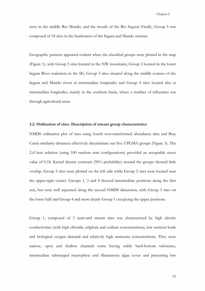
Chapter 2
77
were in the middle Rio Mundo, and the mouth of the Rio Segura) Finally, Group 5 was
composed of 18 sites in the headwaters of the Segura and Mundo streams.
Geographic patterns appeared evident when the classified groups were plotted in the map
(Figure 1), with Group 5 sites located in the NW mountains, Group 2 located in the lower
Segura River mainstem in the SE, Group 3 sites situated along the middle courses of the
Segura and Mundo rivers at intermediate longitudes and Group 4 sites located also at
intermediate longitudes, mainly in the southern basin, where a number of tributaries run
through agricultural areas.
3.2. Ordination of sites. Description of stream group characteristics NMDS ordination plot of sites using fourth root-transformed abundance data and Bray
Curtis similarity distances effectively discriminate our five UPGMA groups (Figure 3). The
2-d best solution (using 100 random start configurations) provided an acceptable stress
value of 0.18. Kernel density contours (90% probability) around the groups showed little
overlap. Group 5 sites were plotted on the left side while Group 2 sites were located near
the upper-right corner. Groups 1, 3 and 4 showed intermediate positions along the first
axis, but were well separated along the second NMDS dimension, with Group 3 sites on
the lower half and Group 4 and more clearly Group 1 occupying the upper positions.
Group 1, composed of 3 semi-arid stream sites was characterized by high electric
conductivities (with high chloride, sulphate and sodium concentrations), low nutrient loads
and biological oxygen demand and relatively high ammonia concentrations. They were
narrow, open and shallow channels some having stable hard-bottom substrates,
intermediate submerged macrophyte and filamentous algae cover and presenting low

Chapter 2
78
diversity and evenness values. Nevertheless, broad environmental differences existed
between these three sites (See Table 1 for a detailed description of physicho-chemical,
climatic, community and habitat variables in each cluster).
Group 2 was characterized by the lowest water quality values (Table 1). Climatic variables
were typical of arid or semi-arid environments, with the highest mean annual temperatures
and potential evapotranspiration among the study sites and annual rainfall values close to
300 mm. They were wide and deep open channels located in wide valleys. Current velocity
was very slow. Substrate was highly instable and silt-dominated while UPOM was the main
sediment organic fraction. Aquatic vegetation cover was low. Macroinvertebrate
communities were characterized by the lowest richness and diversity values.
Group 3 sites were characterized by semi-arid climate, low altitude, relatively high water
quality and low mineralization. Dominant substrate was loose gravel and CPOM was the
main organic sediment fraction. They were wide and deep reaches located in wide valleys
with open canopies. Current velocity was moderate. Aquatic vegetation was almost
inexistent while riparian corridors were well structured. Macroinvertebrate communities
showed low taxa richness and intermediate evenness and diversity values.
Group 4. The main characteristics of this group were: low orders, middle altitudes,
intermediate aridity; moderate water quality (good oxygenation, moderate conductivities
and mineralization, relatively low nutrient loads, suspended solids and BOD5, and
moderate ammonia and nitrite contents). Habitat was characterized by relatively wide and
shallow channels with low to moderate current velocity. Substrate was sandy and CPOM
was the main organic fraction. Submerged macrophytes were moderately abundant. Taxa
richness and Shannon diversity values were high while Pielou evenness showed
intermediate values.

Chapter 2
79
Figure 2. Group average clustering (UPGMA) dendrogram of the study sites based on their Bray-Curtis similarities. Sites are labelled with numbers (1 to 5) identifying
stream groups.
1 1 1 2 2 2 2 2 2 2 2 2 2 2 2 2 2 2 2 2 2 2 2 3 3 3 3 3 3 3 3 3 3 3 3 3 3 3 3 3 3 3 3 3 3 3 3 3 3 3 3 3 4 4 4 4 4 4 4 4 4 4 4 4 4 4 4 4 4 5 5 5 5 5 5 5 5 5 5 5 5 5 5 5 5 5 5
100
80
60
40
20
0

Chapter 2
80
5
4
3
12
GROUPS
Stress= 0.18
5
4
3
12
GROUPS
5
4
3
12
GROUPS
Stress= 0.18
Figure 3. Non-metric Multiple Dimensional Scaling (MDS) ordination plot of the study sites based on their Bray-Curtis similarities. Symbols identify the stream groups defined by UPGMA (see legend). Kernel density contours (90%) were plotted for each group of sites.
Group 5 sites were located in high altitude mountainous conifer-forested areas inside or
very near the Sierra de Cazorla, Segura and Las Villas nature reserve, in the more humid
NW part of the basin (Figure 1). Climate was characterized by relatively low mean annual
temperature and high annual rainfall (close to 700 mm). Water quality variables reached
their best relative values in this group, with very low values (relative to our natural regional
standards) of mineralization, nutrient contents, suspended solids and BOD5, nitrite and
ammonia. Moderately narrow and shallow stretches located in V-shaped valleys formed this
group of sites. Cobbles and boulders were the main substrate types and CPOM dominated
the organic fraction. Submerged macrophytes were scarce while filamentous algae cover
was moderate. There appeared some bryophytes as well. Riparian vegetation was
dominated by trees. Mean taxa richness (with 17 taxa more than group 4, 35 more than

Chapter 2
81
group 3 and 39 more than group 2), diversity and evenness reached their peak values in
these sites.
3.3. Environmental variables explaining community patterns The BVSTEP procedure identified a 5 variables subset giving the highest correlation (ρw =
0.478, see Table 2). However, a second subset identified by this technique that gave a
similar correlation (ρw = 0.475) included only 3 variables (dissolved oxygen, electric
conductivity and altitude) and was therefore considered the most useful model. Moreover,
these three variables were present in all 6 subsets identified. Adding two more variables,
nitrate and annual rainfall, correlation was minimally improved, while when 7, 10 or 12
variables were selected, correlations decreased. Variables included in each model are listed
Table 2. Six best subsets results found by BVSTEP on 28 environmental variables explaining macroinvertebrate patterns. Correlation coefficient for each subset (ρw) is indicated. Variable codes can be found in Table 1.
Subconjuntos de variablesNº de variables 5 3 12 10 7 3
Oxy Oxy Stemp Stemp Oxy E-conE-con E-con Oxy Oxy E-con ChODNO3
- Alt E-con E-con Alk AltAlt NO3
- NO3- Width
P Alk Alk SubSizValley SubSiz AltCurrent SubMac PSubSiz FilAlgSubMac AltFilAlg PAltP
Correlación (ρ w ) 0.478 0.475 0.473 0.473 0.466 0.459

Chapter 2
82
in Table 2. Geo-climatic variables (altitude, air temperature and mean annual precipitation)
and water quality (electric conductivity, dissolved oxygen and nitrate) were the most
important factors explaining macroinvertebrate patterns. Among the habitat variables
(present only in the larger subsets), channel width, valley width, substrate size, current
velocity, submerged macrophyte and filamentous algae were selected.
Canonical correspondence analysis ordination plot was fairly similar to the MDS one, with
the classified site groups occupying approximately the same relative positions.
Nevertheless, two extreme outliers were identified in the CCA plot: Site 61, located near
Group 5 sites, was classified as a polluted site (Group 2) according to the community
because it is located in a reservoir, and Site 53, the mouth of the Segura River, biologically
classified as a Group 4 site but now positioned as a polluted site due to environmental
constraints apparently not affecting the community.
The environmental variables used in the analysis are represented in the biplot (Figure 4) by
arrows, which point in the direction of maximum change in the value of the associated
variable. The arrowhead co-ordinates on each axis are essentially the correlations of the
environmental variable with that ordination axis. The length of the arrow is therefore
proportional to the maximum rate of change for the variable, so those variables with
relatively short arrows do not vary much across the ordination plot and therefore were not
represented for clarity in Figure 4.
The two first CCA axes explained 36.3% of the species-environment relationship. The
Monte Carlo tests (999 permutations) showed that axis 1 and all the axes were statistically
significant (p≈0.001). Interset correlations of environmental variables with CCA
environmental axes were as follow: Axis 1, that accounted for 24.8 % of variance in of the
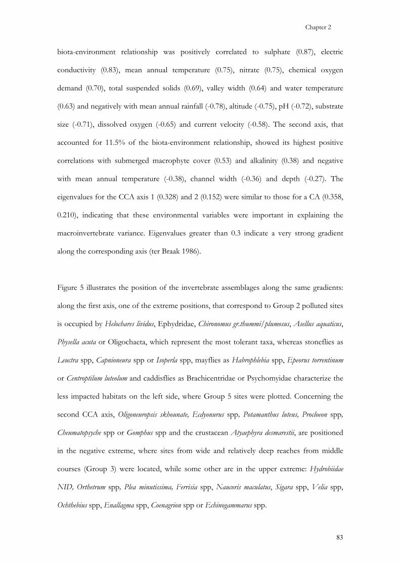
Chapter 2
83
biota-environment relationship was positively correlated to sulphate (0.87), electric
conductivity (0.83), mean annual temperature (0.75), nitrate (0.75), chemical oxygen
demand (0.70), total suspended solids (0.69), valley width (0.64) and water temperature
(0.63) and negatively with mean annual rainfall (-0.78), altitude (-0.75), pH (-0.72), substrate
size (-0.71), dissolved oxygen (-0.65) and current velocity (-0.58). The second axis, that
accounted for 11.5% of the biota-environment relationship, showed its highest positive
correlations with submerged macrophyte cover (0.53) and alkalinity (0.38) and negative
with mean annual temperature (-0.38), channel width (-0.36) and depth (-0.27). The
eigenvalues for the CCA axis 1 (0.328) and 2 (0.152) were similar to those for a CA (0.358,
0.210), indicating that these environmental variables were important in explaining the
macroinvertebrate variance. Eigenvalues greater than 0.3 indicate a very strong gradient
along the corresponding axis (ter Braak 1986).
Figure 5 illustrates the position of the invertebrate assemblages along the same gradients:
along the first axis, one of the extreme positions, that correspond to Group 2 polluted sites
is occupied by Helochares lividus, Ephydridae, Chironomus gr.thummi/plumosus, Asellus aquaticus,
Physella acuta or Oligochaeta, which represent the most tolerant taxa, whereas stoneflies as
Leuctra spp, Capnioneura spp or Isoperla spp, mayflies as Habrophlebia spp, Epeorus torrentinum
or Centroptilum luteolum and caddisflies as Brachicentridae or Psychomyidae characterize the
less impacted habitats on the left side, where Group 5 sites were plotted. Concerning the
second CCA axis, Oligoneuropsis skhounate, Ecdyonurus spp, Potamanthus luteus, Procloeon spp,
Cheumatopsyche spp or Gomphus spp and the crustacean Atyaephyra desmarestii, are positioned
in the negative extreme, where sites from wide and relatively deep reaches from middle
courses (Group 3) were located, while some other are in the upper extreme: Hydrobiidae
NID, Orthetrum spp, Plea minutissima, Ferrisia spp, Naucoris maculatus, Sigara spp, Velia spp,
Ochthebius spp, Enallagma spp, Coenagrion spp or Echinogammarus spp.

Chapter 2
84
Sulph
E-CondP
T
Altitude
Nitrate
pH
SubSiz
ChOD
SS
O2
Current
Alk
Depth
Width
SubMac
-2.5 +3.0
-2.0
+2.5
Sulph
E-CondP
T
Altitude
Nitrate
pH
SubSiz
ChOD
SS
O2
Current
Alk
Depth
Width
SubMac
-2.5 +3.0
-2.0
+2.5
5
4
3
12
GROUPSSulph
E-CondP
T
Altitude
Nitrate
pH
SubSiz
ChOD
SS
O2
Current
Alk
Depth
Width
SubMac
-2.5 +3.0
-2.0
+2.5
Sulph
E-CondP
T
Altitude
Nitrate
pH
SubSiz
ChOD
SS
O2
Current
Alk
Depth
Width
SubMac
-2.5 +3.0
-2.0
+2.5
5
4
3
12
GROUPS
5
4
3
12
GROUPS
Figure 4. Canonical correspondence analysis (CCA) ordination biplot showing study sites and environmental variables vectors (shorter vectors were eliminated for clarity). Again, site symbols identify the stream groups defined by UPGMA (see legend).
They occupied relative positions in the CCA that corresponded to groups 1 and 4.
3.4. Indicator taxa The IndVal method using our 126 taxa x 87 sites data set and 9999 permutations found
some good indicators for the macroinvertebrate-based stream typology defined by
UPGMA classification (Figure 6). In general, among the identified indicators, Coleoptera
was the dominant order with twelve taxa, followed by Diptera and Ephemeroptera – seven
taxa each –, Trichoptera – six taxa –, Plecoptera and Odonata – five taxa each –,
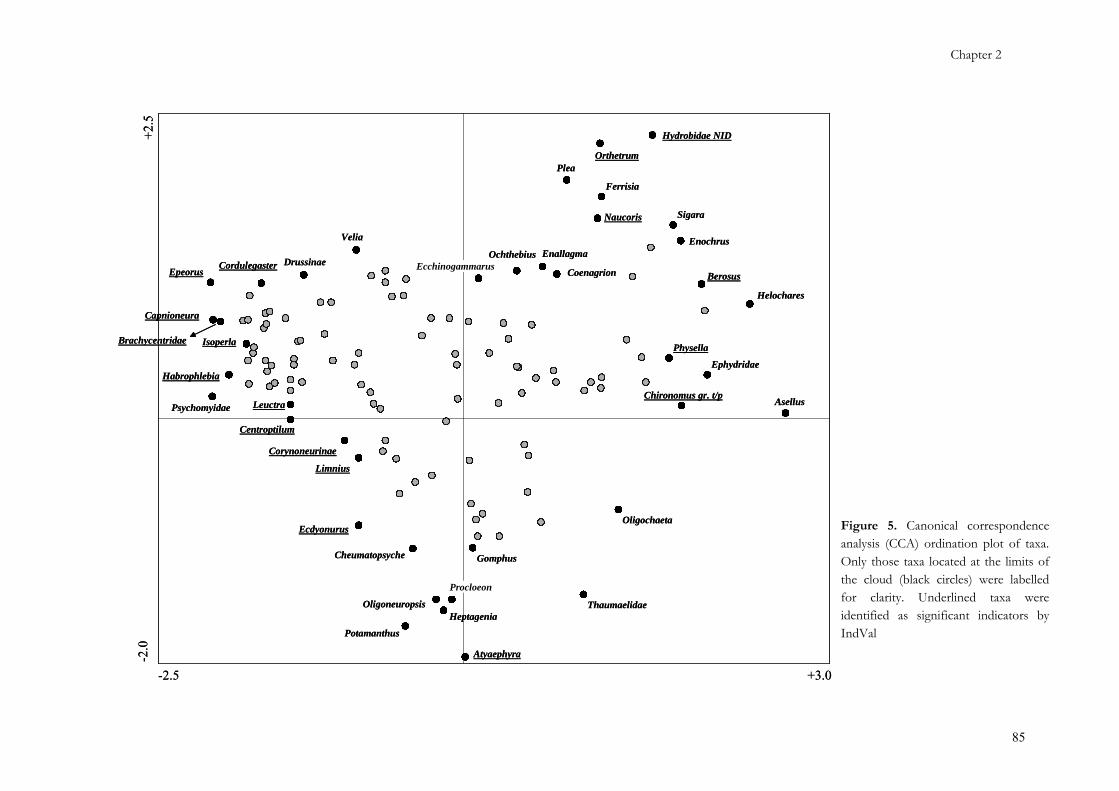
Chapter 2
85
-2.5 +3.0
-2.0
+2.5
Helochares
Epeorus
Psychomyidae
Capnioneura
Ephydridae
Berosus
Habrophlebia
Chironomus gr. t/p
Enochrus
Brachycentridae Isoperla
Sigara
Physella
Cordulegaster
Hydrobidae NID
Centroptilum
Drussinae
Oligochaeta
Ferrisia
Orthetrum
Naucoris
Thaumaelidae
Corynoneurinae
Velia
Ecdyonurus
Limnius
Plea
Potamanthus
Cheumatopsyche
OligoneuropsisHeptagenia
Gomphus
Atyaephyra
Asellus
EcchinogammarusOchthebius Enallagma
Coenagrion
Leuctra
Procloeon
Figure 5. Canonical correspondence analysis (CCA) ordination plot of taxa. Only those taxa located at the limits of the cloud (black circles) were labelled for clarity. Underlined taxa were identified as significant indicators by IndVal

Chapter 2
86
Mollusca and Heteroptera – four taxa – and Decapoda or Tricladida both with one
indicator.
At the second level, where the three sites forming Group 1 were separated, IndVal
identified 10 indicator taxa for this group. Some of them were very good examples of
characteristic taxa (significant IV around 90%). as Hydrobiidae (unknown genera), Naucoris
maculatus, Hydrometra stagnorum or Orthetrum spp. Only one taxon, the midge subfamily
Orthocladiinae (IV=99.7), was found to be a significant indicator of the remaining sites at
the same division level. At the third cluster division, where heavily polluted sites forming
Group 2 were split up, only one significant indicator was found for this cluster, the midge
species group Chironomus gr. thummi/plumosus. Two common mayfly taxa, Caenis spp and
Baetis spp and the caddisfly Hydropsyche spp were indicative of the remaining sites. The
fourth cluster division separated the Group 3 sites, with the crustacean Atyaephyra desmarestii
as their only one indicator taxa. Group 4 and Group 5 were characterized by Simuliidae,
Haliplus spp and Nepa cinerea. Finally, Group 4 characteristic taxa showed relatively low
indicator values, ranging from 30.5 to 44.4. Group 5 was the cluster with the bigger
indicator taxa set (up to 39 significant indicators, with IV ranging from 31.8 to 92.8). It
comprised up to ten coleopterans, seven ephemeropterans, six trichopterans, six dipterans,
five plecopterans, four odonatans and one triclad (Figure 6).
4. Discussion Results are in accord with previous works from the basin where the main trends showed by
aquatic biota were dominated by factors such as electric conductivity and altitude, linked to
a NW-SE geographic and climatic gradient.

Chapter 2
87
B
ray-
Cur
tissi
mila
rity
1520
2530
35
O rth o c la d iin a e (9 9 .6 5 )
C h ir o n o m u s (7 3 .0 8 )(g r th u m m i, p lu m o s u s )
C a e n is (9 0 .2 7 )B a e tis (8 9 .0 0 )
H y d r o p sy c h e (6 5 .9 6 )
S im u liid a e (6 8 .4 6 )H a lip lu s (5 0 .8 3 )
N e p a (4 8 .5 4 )
2
3
4
5
1
H y d ro b iid a e u .g e n . (9 7 .5 2 )N a u c o r is (9 1 .2 0 )
H y d ro m e tr a (8 9 .9 5 )O r th e tr u m (8 6 .5 8 )N o to n e c ta (5 9 .1 6 )
H e lio c o r ix a (4 7 .7 5 )A n iso p s (4 6 .9 1 )
G ro u p 1
G ro u p 2
A ty a e p h ir a (3 4 .9 6 )
G ro u p 3
P o ta m o p y r g u s (4 4 .3 6 )P h y s e lla (4 4 .1 9 )
A u lo n o g y ru s (3 7 .4 5 )M e r c u r ia (3 5 .6 7 )
B e r o su s (3 0 .5 0 )
G ro u p 4
L e u c tra (9 2 .8 0 )E lm is (8 3 .8 1 )
E c d y o n u r u s (8 2 .7 2 )S tr a t io m y id a e (8 2 .6 8 )
E p h e m e r e lla (7 9 .0 4 )O u lim n iu s (7 7 .5 0 )
L im n iu s (7 7 .0 2 )I s o p e r la (7 5 .4 5 )
L im o n iid a e (7 4 .6 5 )H y d r a e n a (7 2 .2 2 )
R io lu s (6 5 .7 5 )E s o lu s (6 5 .6 0 )
R h y a c o p h y la (6 5 .2 9 )
H a b ro le p to id e s (6 1 .0 4 )L im n e p h il in a e (5 0 .0 0 )
B ra c h y c e n tr id a e (4 9 .6 0 )C a lo p te r y x (4 9 .5 5 )T a b a n id a e (4 4 .5 8 )
S e r ic o s to m a tid a e (4 3 .5 9 )C o r d u le g a s te r (4 3 .5 2 )
O n y c h o g o m p h u s (6 0 .6 7 )O r e c to c h ilu s (6 0 .2 9 )
P e r la (5 9 .6 6 )P r o to n e m u r a (5 8 .5 1 )
A th e r ic id a e (5 5 .7 5 )C e n tr o p tilu m (5 4 .7 2 )
G ro u p 5
P o m a tin u s (5 4 .6 3 )R h ith r o g e n a (4 3 .0 0 )
N o r m a n d ia (4 2 .3 8 )L a c c o b iu s (4 2 .1 7 )
B o y e r ia (4 2 .0 4 )E m p id id a e (4 0 .5 8 )H y d r o p ti la (4 0 .4 0 )
C o r y n o n e u r in a e (3 9 .1 8 )B e ra e id a e (3 8 .8 9 )
E p e o r u s (3 3 .3 3 )C a p n io n e u r a (3 3 .3 3 )
H a b r o p h le b ia (3 3 .2 2 )P o ly c e l is (3 1 .8 0 )
Bra
y-C
urtis
sim
ilarit
y
1520
2530
3515
2025
3035
O rth o c la d iin a e (9 9 .6 5 )
C h ir o n o m u s (7 3 .0 8 )(g r th u m m i, p lu m o s u s )
C a e n is (9 0 .2 7 )B a e tis (8 9 .0 0 )
H y d r o p sy c h e (6 5 .9 6 )
S im u liid a e (6 8 .4 6 )H a lip lu s (5 0 .8 3 )
N e p a (4 8 .5 4 )
2
3
4
5
1
H y d ro b iid a e u .g e n . (9 7 .5 2 )N a u c o r is (9 1 .2 0 )
H y d ro m e tr a (8 9 .9 5 )O r th e tr u m (8 6 .5 8 )N o to n e c ta (5 9 .1 6 )
H e lio c o r ix a (4 7 .7 5 )A n iso p s (4 6 .9 1 )
G ro u p 1G ro u p 1
G ro u p 2G ro u p 2
A ty a e p h ir a (3 4 .9 6 )
G ro u p 3
A ty a e p h ir a (3 4 .9 6 )
G ro u p 3
P o ta m o p y r g u s (4 4 .3 6 )P h y s e lla (4 4 .1 9 )
A u lo n o g y ru s (3 7 .4 5 )M e r c u r ia (3 5 .6 7 )
B e r o su s (3 0 .5 0 )
G ro u p 4
P o ta m o p y r g u s (4 4 .3 6 )P h y s e lla (4 4 .1 9 )
A u lo n o g y ru s (3 7 .4 5 )M e r c u r ia (3 5 .6 7 )
B e r o su s (3 0 .5 0 )
G ro u p 4
L e u c tra (9 2 .8 0 )E lm is (8 3 .8 1 )
E c d y o n u r u s (8 2 .7 2 )S tr a t io m y id a e (8 2 .6 8 )
E p h e m e r e lla (7 9 .0 4 )O u lim n iu s (7 7 .5 0 )
L im n iu s (7 7 .0 2 )I s o p e r la (7 5 .4 5 )
L im o n iid a e (7 4 .6 5 )H y d r a e n a (7 2 .2 2 )
R io lu s (6 5 .7 5 )E s o lu s (6 5 .6 0 )
R h y a c o p h y la (6 5 .2 9 )
H a b ro le p to id e s (6 1 .0 4 )L im n e p h il in a e (5 0 .0 0 )
B ra c h y c e n tr id a e (4 9 .6 0 )C a lo p te r y x (4 9 .5 5 )T a b a n id a e (4 4 .5 8 )
S e r ic o s to m a tid a e (4 3 .5 9 )C o r d u le g a s te r (4 3 .5 2 )
O n y c h o g o m p h u s (6 0 .6 7 )O r e c to c h ilu s (6 0 .2 9 )
P e r la (5 9 .6 6 )P r o to n e m u r a (5 8 .5 1 )
A th e r ic id a e (5 5 .7 5 )C e n tr o p tilu m (5 4 .7 2 )
G ro u p 5
P o m a tin u s (5 4 .6 3 )R h ith r o g e n a (4 3 .0 0 )
N o r m a n d ia (4 2 .3 8 )L a c c o b iu s (4 2 .1 7 )
B o y e r ia (4 2 .0 4 )E m p id id a e (4 0 .5 8 )H y d r o p ti la (4 0 .4 0 )
C o r y n o n e u r in a e (3 9 .1 8 )B e ra e id a e (3 8 .8 9 )
E p e o r u s (3 3 .3 3 )C a p n io n e u r a (3 3 .3 3 )
H a b r o p h le b ia (3 3 .2 2 )P o ly c e l is (3 1 .8 0 )
Figure 6. UPGMA classification dendrogram showing the significant indicator taxa with their indicator value (in brackets) calculated by the INDVAL program for each of the cluster divisions.

Chapter 2
88
Macroinvertebrate communities from the Segura River basin are still poorly known.
Despite some local government reports or sparse faunistic references on certain taxa
(Millan et al., 1988; 1993; Gil et al., 1990; Ubero-Pascal al., 1998; Bonada et al., 2004), little
information about general distribution, environmental factors or any other ecological
aspect of these stream assemblages has been published to the date (but see Mellado et al.,
2002; Vivas et al., 2004). We present important baseline information about the
environmental variables affecting the distribution patterns of macroinvertebrate
communities in our region. Moreover, a long-term information point (we treated 1987
data) has been established for comparative studies in the future.
4.1. Site classification and ordination. Indicator taxa Freshwater conservation strategies and monitoring programmes typically rely on
classification of sites based on a single biotic group, most typically benthic
macroinvertebrates. Our site classification (and a posteriori ordination) resulted in four
main distinguishable classes. Physicho-chemical, geo-climatic, habitat and community
variables allowed us to basically describe each group. Three of the groups were each
positioned in a distinct portion of the longitudinal gradient of the Segura and Mundo rivers
(Groups 5 –headwaters-, 3 –middle courses- and 2 –lower courses-, Figure 1). Group 4 was
composed of tributaries flowing into middle courses of the main axis. Mellado et al. (2002)
found a very similar classification using family level presence-absence data across sixty sites
in 1998, although one more group (“Group 5” in Mellado et al., 2002) was defined, mainly
composed of small saline streams that were not sampled in 1987 (this study). Two of the
three sites from Group 1 here were part of that group in 1998.

Chapter 2
89
Faunal composition and community structure was markedly distinct among the classified
groups, as the indicator value method (IndVal) and the CCA species plot showed. The
IndVal method (Dufrêne and Legendre, 1997) enabled the identification of indicator taxa
for each of the 5 groups and cluster hierarchy levels. Coleoptera was the most represented
group. The indicator value of aquatic beetles has been pointed out in numerous works
(Ribera and Foster, 1993; Ribera, 2000; Sánchez-Fernández et al., 2004). The group that
showed most of the indicator taxa was Group 5, with almost 40 taxa. They were mostly
good water quality indicators, stenotypic species typical of high altitude ranges and
relatively low temperature tolerance such as the majority of EPT taxa, elmid beetles and
some dipterans and odonatans. Stratiomyidae, a dipteran family usually known as a tolerant
group (Alba-Tercedor and Sánchez Ortega, 1988; Chessman, 1995) was found as a very
good indicator (IV=82.7%) for these streams, what we could justify because of the
abundance of the genus Oxycera in semi-pristine streams from the upper catchment.
Group 4 indicators showed lower IVs. They were more eurytopic taxa, but were more
abundant in these systems. There were three aquatic snails, Physella acuta and Potamopyrgus
antipodarum, usually typical of stagnant waters or low flow streams and with very wide
geographical distributions and Mercuria emiliana, an interesting hydrobid snail that is
common in mineralized streams. Two water beetles: Berosus spp, with most of species with
marked preferences for middle altitudes, shallow or lentic habitats and moderate to high
mineralization (Sánchez-Meca et al., 1992), and Aulonogyrus striatus, the most eurythermic
gyrinid species within the Segura River basin (Millan et al., 1996).
The decapod Atyaephyra desmarestii was found as an indicator of the middle courses of
Group 3. This organism has shown preference for relative good water quality and a variety
Chapter 2
90
of habitats, including reservoirs and channelizated reaches or rice fields (Micha et al., 1985;
Rinderhagen et al., 2000; Fidalgo and Gerhardt, 2003).
The well known pollution tolerant taxa Chironomus gr. thummi/plumosus was the only
indicator taxa for polluted lower reaches of Group 2. This species group has long been
reported in numerous studies as one of the most pollution tolerant taxa (e.g. Hilsenhoff,
1987; Zamora-Muñoz and Alba-Tercedor, 1996; Walsh et al., 2001; Janssens de Bisthoven
and Gerhardt, 2003).
Group 1 sites were characterized by relatively high IVs for some Heteroptera (Naucoris
maculatus, Hydrometra stagnorum, Notonecta spp, Heliocorixa vermiculata and Anisops spp), one
artificial taxa designated as Hydrobiidae u.gen. (too small to identify) and Orthetrum spp.
Their position in the CCA (on the right upper corner) indicated preference for shallow
streams with low flow, high macrophyte cover and high mineralization and nitrate
contents. Nevertheless, with only three sites within this group in this study we have limited
data in characterizing species-habitat relationships.Only groups 1, 2 and 5 presented values
over 70%, a threshold showed by McGeoch et al. (2002) to remain consistent among
different studies. It is important to note that a verification study (with new data collection
in 1998) of the indicator taxa found in this work will be carried out to achieve a higher
confidence (sensu McGeoch et al. 2002).
4.2 Environmental constraints Understanding community patterns is important to manage target ecosystems. Invertebrate
community structure reflects the influence of many variables, and discrete influences are
difficult to identify. We used classification and ordination to examine multivariate
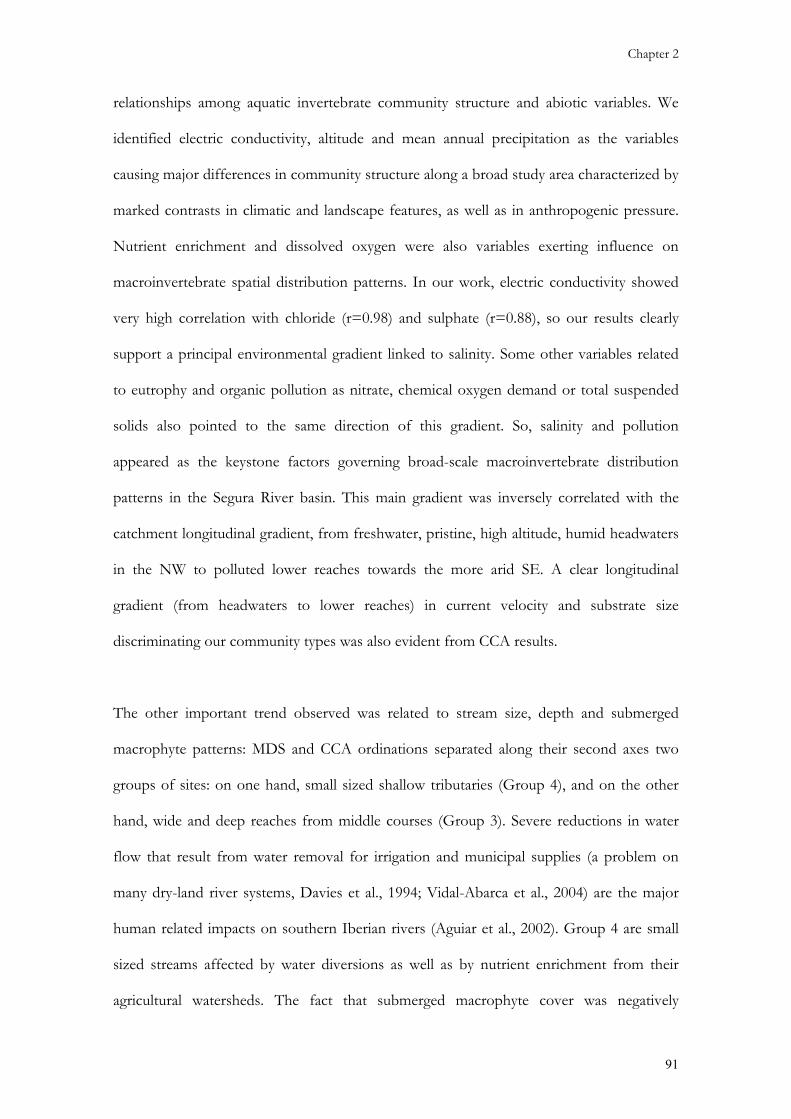
Chapter 2
91
relationships among aquatic invertebrate community structure and abiotic variables. We
identified electric conductivity, altitude and mean annual precipitation as the variables
causing major differences in community structure along a broad study area characterized by
marked contrasts in climatic and landscape features, as well as in anthropogenic pressure.
Nutrient enrichment and dissolved oxygen were also variables exerting influence on
macroinvertebrate spatial distribution patterns. In our work, electric conductivity showed
very high correlation with chloride (r=0.98) and sulphate (r=0.88), so our results clearly
support a principal environmental gradient linked to salinity. Some other variables related
to eutrophy and organic pollution as nitrate, chemical oxygen demand or total suspended
solids also pointed to the same direction of this gradient. So, salinity and pollution
appeared as the keystone factors governing broad-scale macroinvertebrate distribution
patterns in the Segura River basin. This main gradient was inversely correlated with the
catchment longitudinal gradient, from freshwater, pristine, high altitude, humid headwaters
in the NW to polluted lower reaches towards the more arid SE. A clear longitudinal
gradient (from headwaters to lower reaches) in current velocity and substrate size
discriminating our community types was also evident from CCA results.
The other important trend observed was related to stream size, depth and submerged
macrophyte patterns: MDS and CCA ordinations separated along their second axes two
groups of sites: on one hand, small sized shallow tributaries (Group 4), and on the other
hand, wide and deep reaches from middle courses (Group 3). Severe reductions in water
flow that result from water removal for irrigation and municipal supplies (a problem on
many dry-land river systems, Davies et al., 1994; Vidal-Abarca et al., 2004) are the major
human related impacts on southern Iberian rivers (Aguiar et al., 2002). Group 4 are small
sized streams affected by water diversions as well as by nutrient enrichment from their
agricultural watersheds. The fact that submerged macrophyte cover was negatively

Chapter 2
92
correlated with stream width and depth can be explained as middle course sites from
Group 3 usually are affected by flow regulation and channelization, both factors preventing
the normal develop of aquatic plants (Armitage and Pardo, 1995; Wood et al., 1999).
Results indicate that the most influential variables for community structure were variables
that usually operate at a regional scale, affected by climatic and/or geological patterns
(mineralization, altitude, rainfall) or land use activities (eg. Nitrate). Some local physical
habitat attributes as channel width, substrate size or current velocity (also governed by
catchment scale features as geology, altitude or slope) were also important factors although
to a lesser extent. Our findings suggest that the broad scale patterns observed in
macroinvertebrate assemblages are not determined solely by local mechanisms acting
within assemblages, but mainly result from processes operating at larger spatial scales. The
integration of different spatial scales may be the key to increasing our understanding of the
complex interacting factors that determine community composition.
On the other hand, variables such as altitude, geology and land use practices are highly
intercorrelated. Another confounding effect could be the fact that habitat quality in our
lowland urban watersheds is usually poor due to several interacting factors such as
sedimentation from construction works, channelization, damming, bank erosion, loss of
riparian habitats, etc. All of these have negative consequences for biological communities.
Moreover, increasing conductivity and salinity from land use practices potentially confound
the effect of natural longitudinal and salinity gradients. This make difficult to accurately
assess the effect of one single variable on a broad complex catchment. In addition, many of
these factors began affecting streams at the onset of human settlement, leading one to
conclude that current ecosystem health may reflect centuries of pollution, degradation, and
in some cases recovery (Nedeau et al. 2003). Despite these potentially confounding effects,

Chapter 2
93
clear differences were nevertheless detected between communities under different
environmental scenarios. Properly designed experiments are required to disentangle the
array of confounding factors that influence community patterns in the Segura river basin.
5. References Aboal, M. 1989. Epilithic algal communities from River Segura Basin, Southeastern Spain. Archiv für Hydrobiologie 116:113-124 Aguiar, F. C., M.T. Ferreira, P. Pinto. 2002. Relative influence of environmental variables on macroinvertebrate assemblages from an Iberian basin. Journal of the North American Benthological Society 21:43-53. Alba-Tercedor, J.; Sánchez-Ortega, A. 1988. Un método rápido y simple para evaluar la calidad biológica de las aguas corrientes basado en el de Hellawell (1978). Limnética, 4: 51-56. Allan, J. D. 1995. Stream Ecology: Structure and Function of Running Waters. Chapman and Hall, New York, NY, USA. Armitage, P.D.; I. Pardo, 1995. Impact assessment of regulation at the reach level using macroinvertebrate information from mesohabitats. Regulated Rivers: Research and Management 10: 147–158. Bonada, N., Zamora-Muñoz, C., Rieradevall, M.; Prat, N. 2004. Trichoptera (Insecta) collected in Mediterranean river basins of the Iberian Peninsula: taxonomic remarks and notes on ecology. Graellsia, 60(1): 41-69 Boulton, A. J. ; P. S. Lake, 1992. The ecology of two intermittent streams in Victoria, Australia. II. Comparisons of faunal composition between habitats, rivers and years. Freshwater Biology 27: 99–121. Boyero, L. 2003. Multiscale patterns of spatial variation in stream macroinvertebrate communities. Ecological Research 18: 365–379 Brewin P.A., Newman T.M.L.; Ormerod S.J. 1995. Patterns of macroinvertebrate distribution in relation to altitude, habitat structure and land use in streams of the Nepalese Himalaya. Archiv für Hydrobiologie, 135, 79–100.

Chapter 2
94
Céréghino, R., J.L. Giraudel; A. Compin. 2001. Spatial analysis of stream invertebrates distribution in the Adour-Garonne drainage basin (France), using Kohonen self organizing maps. Ecological Modelling 146: 167–180. Chessman, B.C., 1995. Rapid assessment of rivers using macroinvertebrates: a proceedure based on habitat-specific sampling, family-level identification and a biotic index. Australian Journal of Ecology 18:117–143. Clarke K. R. 1993. Non-parametric multivariate analyses of change in community structure. Australian Journal of Ecology 18, 117–143. Clarke K. R.; Ainsworth M. 1993. A method of linking multivariate community structure to environmental variables. Marine Ecology Progress Series 92: 205–219. Clarke K.R., Warwick R.M. 1994. Change in marine communities: an approach to statistical analysis and interpretation. Plymouth Marine Laboratory, Plymouth Clarke K.R., Warwick R.M. 1998. Quantifying structural redundancy in ecological communities. Oecologia 113: 278-289 Davies, B. R., Thoms, M. C., Walker, K. F., O’keefe, J. H.; Gore, J. A. 1994. Dryland rivers: their ecology, conservation and management. Pages 484–511 in P. Calow and G. Petts (editors). The rivers handbook, Volume 2. Blackwell Scientific Publications, London, UK. Degani, G., G. N. Herbst, R. Ortal, H. J. Bromley, D. Levanon, Y. Netzer, N. Harari, H. Glazman. 1993. Relationship between current velocity, depth and the invertebrate community in a stable river system. Hydrobiologia 263, 163-172. Dufrene, M.; Legendre, P. 1997. Species assemblages and indicator species: the need for a flexible asymmetrical approach. Ecological Monographs 67: 345–367. Duggan, I.C., Green, J.D.; Shiel, R.J. 2001. Distribution of rotifers in North Island, New Zealand, and their potential use as bioindicators of lake trophic state Hydrobiologia 446/447: 155–164. Fidalgo M.L., Gerhardt A., 2003. Distribution of the freshwater shrimp, Atyaephyra desmarestii (Millet, 1831) in Portugal (Decapoda, Natantia). Crustaceana, 75(11): 1375-1385. Gauch, H.G. 1982. Multivariate analysis in community ecology. Cambridge University Press, Cambridge. UK.

Chapter 2
95
Gil, E., Montes, C., Millan, A. and Soler, A.G. 1990: Los coleópteros acuáticos (Dryopidae and Elmidae) de la cuenca del río Segura. SE de la Península Ibérica. Anales de Biología, 16: 23-31. Gómez, R., Hurtado, I., Suárez, M.L.; Vidal-Abarca, M.R. 2005. Ramblas in Southeast Spain: threatened and valuable ecosystems Aquatic Conservation. Marine and Freshwater Ecosystems, (in press) Hawkes H.A. 1975. River zonation and classification. Pages 312-374 in B.A. Whitton, ed. River ecology. Blackwell, London, UK. Hawkins, C.P. ; Vinson, M.R. 2000. Weak correspondence between classifications and stream invertebrate assemblages: implications for bioassessment. Journal of the North American Benthological Society 19(3): 501-517. Heino, J., Muotka, T.; Paavola, R. 2003 Determinants of macroinvertebrate diversity in headwater streams: regional and local influences Journal of Animal Ecology 72: 425–434 Hilsenhoff, W.L. 1987. An improved biotic index of organic stream pollution. Great Lakes Entomologist 20:31-40. Hynes, H.B.N. 1970. The Ecology of Running Waters. University of Toronto Press, Toronto, Ont., Canada. Janssens de Bisthoven, L.; Gerhardt, A. 2003. Chironomidae (Diptera, Nematocera) FAUNA in three small streams of Skania, Sweden. Environmental Monitoring and Assessment 83: 89–102. Kruskal, J.B., and Wish. M. 1978. Multidimensional scaling. Sage Publications, Beverly Hills, California. Magdych W.P. 1984. Salinity stress along a complex river continuum: effects on mayfly (Ephemeroptera) distributions. Ecology, 65, 1662-1672. Leland, H.V., S.V. Fend. 1998. Benthic invertebrate distribution in the San Joaquín River, California, in relation to physical and chemical factors. Canadian Journal of Fisheries and Aquatic Sciences 55: 1051-1067. McGeoch, M.A. 2002. Bioindicators, in Encyclopedia of Environmetrics, volume 1, pp 186–189. Edited by El-Shaarawi, A.H. and Piegorsch W.W. John Wiley & Sons, Ltd, Chichester McGeoch, M.A.; Chown, S.L., 1998. Scaling up the value of bioindicators. Trends in Ecology and Evolution 13, 2: 46-47.

Chapter 2
96
McGeoch, M.A. Van Rensburg, B.J. and Botes, A. 2002. The verification and application of bioindicators: a case study of dung beetles in a savanna ecosystem. Journal of Applied Ecology 39: 661–672 Mellado, A., Suárez, M.L., Moreno, J.L.; Vidal-Abarca, M.R. 2002. Aquatic macroinvertebrate biodiversity in the Segura River Basin (SE Spain). Verh. Internat. Verein. Limnol. 28 (1157-1162) Micha J.-C., en collaboration avec M. Meurisse-Genin, A. Reydams-Detollenaere, O. Donatti, 1985 - Caractéristiques biologiques de la crevette d'eau douce Atyaephyra desmaresti Millet dans la Meuse. Annls. Limnol., 21, 2, 127-140. Millan, A., Velasco, J., Nieser, N.; Montes, C. 1988. Heteropteros acuáticos (Gerromorpha y Nepomorpha) de la cuenca del río Segura, SE España. Anales de Biología, 15(4) 74-89. Millán, A., Velasco, J.; Soler, A.G. 1993. Los Coleópteros Hydradephaga de la cuenca del río Segura (SE de la Península Ibérica). Estudio corológico. Boletín de la Asociación Española de Entomología, 17(1): 19-39. Millán, A., Velasco, J., Vidal-Abarca, M.R., Suárez, M.L.; Ramírez-Díaz, L. 1996. Distribución espacial de los Adephaga acuáticos (Coleoptera) en la cuenca del río Segura (SE de la Península Ibérica). Limnética, 12(2): 13-29. Minshall, G.W., Petersen, R.C., Jr. 1985. Towards a theory of macroinvertebrate community structure in stream ecosystems. Archiv für Hydrobiologie 104: 49–76. Moreno, J.L., Millan, A., Suarez, M.L., Vidal-Abarca, M.R.; Velasco, J., 1997. Aquatic Coleoptera and Heteroptera assemblages from ephemeral coastal streams (“ramblas”) of south-eastern Spain. Archive fur Hydrobiologie, 141 (1): 93-107 Moreno, J.L., Aboal, M., Vidal-Abarca, M.R.; Suarez, M.L. 2001. Macroalgae and submerged macrophytes from fresh and saline waterbodies of ephemeral streams (“ramblas”) in semiarid south-eastern Spain. Mar. FreshWater Research, 52, 891-905. Naiman, R.J. 1998. Biotic stream classification. Pages 97-119, in R.J. Naiman and R.E. Bilby (Editors). River Ecology and Management: Lessons from the Pacific Coastal Ecoregion. Springer-Verlag, New York. Nedeaua, E.J., Merritt, R.W.; Kaufman, M.G. 2003. The effect of an industrial effluent on an urban stream benthic community: water quality vs. habitat quality. Environmental Pollution 123 : 1–13.

Chapter 2
97
Ormerod, S.J.; Edwards, R. W. 1987. The ordination and classification of macroinvertebrate assemblages in the catchment of the River Wye in relation to environmental factors. Freshwater Biology 17:533–546. Paavola, R., Muotka, T., Virtanen, R., Heino, J.; Kreivi, P. 2003. Are biological classifications of headwater streams concordant across multiple taxonomic groups?. Freshwater Biology 48, 1912–1923. Ribera, I.; Foster, G. 1993. Uso de Coleópteros acuáticos como indicadores biológicos (Coleoptera). Elytron, 6: 61-75. Ribera, I. 2000. Biogeography and conservation of Iberian water beetles. Biological Conservation, 92: 131-150. Rinderhagen, M., Ritterhoff, J.; Zauke, P. 2000. Crustaceans as Bioindicators (pp. 161-194). In: A. Gerhardt (ed.). Biomonitoring of Polluted Water – Reviews on Actual Topics. Trans. Tech. Publications – Scitech Publications, Environmental Research Forum Vol. 9 Sánchez-Fernández, D.; P. Abellán; J. Velasco & A. Millán. 2004. Áreas prioritarias de conservación en la cuenca del río Segura utilizando los coleópteros acuáticos como indicadores. Limnética, 2002, 23(3-4): 209-228. Sánchez-Meca, J. J., Millán, A.; Soler, A. G. 1992. El género Berosus Leach, 1817 (Coleoptera: Hydrophilidae) en la cuenca del río Segura (SE España). Elytron, 6: 91-107. Tate, C.M.; J.S. Heiny. 1995. The ordination of benthic invertebrate communities in the South Platte River Basin in relation to environmental factors. Freshwater Biology 33: 439–454. ter Braak, C.J.F. (1986). Canonical correspondence analysis: a new eigenvector technique for multivariate direct gradient analysis. Ecology 67: 1167-1179. Townsend, C.R., Hildrew A.G. 1994. Species traits in relation to a habitat templet for river systems. Freshwater Biology 31:265–275. Ubero-Pascal, N.A.; Puig, M.A.; Soler, A.G. 1998. Los Efemerópteros de la Cuenca del río Segura (S.E. de España): 1. Estudio faunístico. (Insecta: Ephemeróptera). Boletín de la Asociación Española de Entomología 22 (1-2): 151-170. Vidal-Abarca, M.R.; M.L. Suárez: L. Ramírez-Díaz. 1992. Ecology of spanish semiarid streams. In: Limnology in Spain. (Montes, C.; C. Duarte, Eds.). Limnética. Asociación Española de Limnología. Páginas: 151-160.

Chapter 2
98
Vidal-Abarca, M.R., Gómez, R.; Suárez, M.L. 2004. Los ríos de las regiones semiáridas. Ecosistemas 1 (URL: http//www.aeet.org/ecosistemas/041/revision4.htm) Vinson, M.R. ; Hawkins, C.P. 1998. Biodiversity of stream insects: variation at local, basin, and regional scales. Annu. Rev. Entomol. 43: 271–293. Vivas, S.; Casas, J. J.; Pardo, I.; Robles, S.; Bonada, N.; Mellado, A.; Prat, N.; Alba-Tercedor, J.; Álvarez, M.; Bayo, M. M.; Jáimez-Cuéllar, P.; Suárez, M. L.; Toro, M.; Vidal-Abarca, M. R.; Zamora-Muñoz, C.; Moyá, G. 2004. Aproximación multivariante en la exploración de la tolerancia ambiental de las familias de macroinvertebrados de los ríos mediterráneos del proyecto GUADALMED. Limnetica, 2002, 21(3-4): 149-173 Walsh, C.J., Sharpe, A.K., Breen, P.F.; Sonneman, J.A. 2001. Effects of urbanization on streams of the Melbourne region, Victoria, Australia. I. Benthic macroinvertebrate communities. Freshw. Biol. 46: 535–554. Wood P.J., Armitage P.D., Cannan C.E., Petts G.E. 1999. Instream mesohabitat biodiversity in three groundwater streams under base-flow conditions. Aquatic Conservation: Marine and Freshwater Ecosystems 9: 265–278. Wright, J.F., D. Moss. P.D. Armitage; M.T. Furse. 1984. A preliminary classification of running water sites in Great Britain based on macro-invertebrate species and the prediction of community type using environmental data. Freshwater Biology 14:221-256. Zamora-Muñoz, C. and Alba-Tercedor, J. 1996. Bioassessment of organically polluted Spanish rivers, using a biotic index and multivariate methods. Journal of the North American Benthological Society 15 (3), 332–352.

Chapter 2
99
Appendix 1
Taxonomic unit
TaxaTaxonom
ic unit Taxa
Taxonomic unit (C
ode)Taxa
Taxonomic unit (C
ode)Taxa
Taxonomic unit (C
ode)Taxa
Coleoptera
Aulonogyrus
Heteroptera
Hydrom
etraTrichoptera
Diptera
TipulidaeC
rustaceaA
sellusG
yrinusV
eliaH
ydropsycheLim
oniidaeE
chinogamm
arusO
rectochilusM
icroveliaC
heumatopsyche
Psychodidae
Atyaephyra
Peltodytes
Aquarius
Sericostom
atidaeD
ixidaeA
ustropotamobius
Haliplus
Gerris
Rhyacophyla
Chaoborus
Hydroglyphus
Micronecta
Psychom
yidaeC
ulicidaeM
olluscaG
raptodytesC
ymatia
Brachycentridae
Sim
uliidaeA
ncyllusLaccophylus
Heliocorixa
LeptoceridaeTanypodinae
FerrisiaA
gabusS
igaraB
eraeidaeTanytarsini
Hydrobiidae
IlybiusC
orixaH
ydroptilaC
hironomini
Mercuria
Hydaticus
Aphelocheirus
Agraylea
Chironom
us gr. Thumm
i/ripariusP
otamopyrgus
Yola
Nepa
Limnephilinae
Orthocladiinae
Pseudam
nicolaH
ygrotusA
nisopsD
russinaeThaum
aelidaeLym
naeaH
ydrophilusN
otonectaP
hilopotamidae
Ceratopogonidae
Physella
Stictonectes
Mesovelia
Glossosom
atidaeS
tratiomyidae
Planorbis
Deronectes
Hebrus
Polycentropodidae
Em
pididaeG
yraulusN
ebrioporusN
aucorisPlecoptera
TabanidaeM
elanopsisO
reodytesP
leaN
emoura
Atherycidae
TheodoxusR
hantusP
rotonemura
Ephydridae
Pisidium
Meladem
aEphem
eropteraA
mphinem
uraC
orynoneurinaeD
ytiscusB
aetisThyrrenoleuctra
Anthom
yidaeH
elobdellaC
ybisterC
loeonLeuctra
Ptychopteridae
Dina
LaccobiusP
rocloeonC
apnioneuraS
yrphidaeO
ther groupsH
elocharesC
entroptilumC
apniaD
olichopodidaeTricladida
Enochrus
Epeorus
Perla
Oligochaeta
Hydphidrus
Rhithrogena
Eoperla
Odonata
Nem
atodaB
erosusE
cdyonurusD
inochrasC
alopteryxH
ydracarinaA
nacaenaH
eptageniaIsoperla
Platycnem
isC
oelostoma
TorleyaIsogenus
Pyrrhosom
aH
ydraenaE
phemerella
Chloroperla
IschnuraO
chthebiusC
aenisC
ercionLim
nebiusP
araleptophlebiaC
oenagrionP
omatinus
Habroleptoides
Enallagm
aD
ryopsH
abrophlebiaO
nychogomphus
Potam
ophilusC
horotherpesG
omphus
Elm
isE
phemera
Boyeria
Esolus
Ephoron
Aeschna
Oulim
niusP
otamanthus
Anax
Limnius
Oligoneura
Cordulia
Riolus
Oligoneuropsis
Oxygastra
Norm
andiaS
ympetrum
Hydrochara
Crocothem
isE
lodesO
rthetrumH
elophorusLibellula
Noterus


Chapter 3
Biological and ecological traits of stream macroinvertebrates from a semi-arid
catchment. Patterns along complex environmental gradients


Chapter 3
103
Chapter 3. Biological and ecological traits of stream macroinvertebrates from a semi-arid
catchment. Patterns along complex environmental gradients
Abstract The relationships between biological and ecological traits of macroinvertebrate
communities and environmental attributes measured at different spatial scales was
investigated in various streams with contrasting physical, chemical or landscape level
attributes. We used a newly developed ordination technique, the RLQ analysis (Dolèdec
1996), that links an environmental table (R) with a faunal attributes table (Q) through a
faunal abundance table (L) to provide insights into the relationships between habitat
attributes and biological or ecological traits. We specifically address the following questions:
Are there differences in the suites of biological and ecological traits from streams of
contrasting environmental features?; Which are the principal traits involved in those
possible trends?; Is there a match between certain ecological preferences and some
corresponding life-history traits?; Which are the main environmental factors driving those
differences and at which spatial scales are acting?; Are those differences in concordance
with the River Habitat Templet and other relevant ecological theories?.
A major environmental axis explaining the distribution of communities and their distinctive
biological/ecological features was obtained. This axis included both variables of
anthropogenic pressure (agricultural and urban uses) and natural variability (climatic and
geologic) that are strongly intercorrelated in the study area, with a clear spatial component.
We generally found typical attributes of species from frequently disturbed systems (small
size, polivoltinism, dormancy, ovoviviparity, etc.) in the semi-arid SE part of the study area,
while traits commonly occurring in more stable and favourable environments (big sizes,

Chapter 3
104
merovoltinism, isolated eggs, etc.) were found in mountain forested catchments sites from
the humid NW part.
The natural climatic variation was proposed as a disturbance axis of a theoretical habitat
templet (driven by the more intense disturbance regime typical of semi-arid streams), while
the anthropogenic pressure (mainly driven by intensive agriculture) summed to the natural
increase in salinity due to differential geology was proposed as an adversity axis. Thus, our
principal gradient was supposed as the diagonal of the templet, from the less disturbed
freshwater streams in forested catchments of the humid north-west, to the most disturbed
and often saline streams.
KEYWORDS: Biological traits, Ecological traits, semi-arid stream, macroinvertebrates, SE
Spain, multivariate methods

Chapter 3
105
1. Introduction The distribution and abundance of stream macroinvertebrates are influenced by a variety of
physical and biological factors. Abiotic factors, in particular those related to disturbance
(Resh et al., 1988; Poff, 1992) and habitat heterogeneity, which provide shelter from
disturbance (Sedell et al., 1990; Scarsbrook & Townsend, 1993; Minshall & Robinson,
1998) clearly determine the composition of invertebrate communities. Abiotic factors that
influence community structure differ from system to system and with the spatial scale (Tate
& Heiny, 1995; Vinson & Hawkins, 1998; Boyero, 2003).
On the other hand, already in the 1920s, habitat was clearly seen as a filter for biological
traits, and patterns in these traits were related to spatial habitat variability as well as to
disturbance (Statzner et al., 2001). These ideas were merged by Southwood (1977) in the
“habitat templet concept”. Southwood (1977, 1988) postulates that spatio-temporal habitat
variations provides a “templet” against which differences in fundamental life history and
other species traits result in differential survival and reproduction. Consequently, over
evolutionary time, there should be a correspondence between life history traits and habitat
characteristics. Townsend & Hildrew (1994) developed their “River Habitat Templet” by
predicting trends of traits across spatio-temporal variability gradients. They predicted that
organisms in habitats with high temporal and low spatial variability would be more resilient
and/or more resistant than organisms in habitats with opposite conditions. Temporal
variability refers to the frequency of disturbances whereas spatial variability refers to the
abundance of refugees buffering the effect of disturbances (Townsend & Hildrew, 1994;
Townsend et al., 1997).
Another proposed axis for the habitat template was the “adversity (or favourableness)
axis”, ranging from harsh to rich habitats (Southwood, 1977). In this context, in

Chapter 3
106
continuously harsh environments, owing to physical (e.g. hot springs) or chemical (e.g.
salinity) factors, adapted species would be relatively free of interspecific competition
(Hynes, 1970). Greenslade (1983) termed this kind of selective forces as ‘beyond K’
selection.
Trends of species traits in these habitat templets were usually obvious and often statistically
significant (Resh et al., 1994; Scarsbrook & Townsend, 1993; Statzner et al., 1997;
Townsend et al., 1997; Usseglio-Polatera, 1994). In a complementary way, the traits of a
faunal assemblage can demonstrate some of the characteristics of the environment,
presenting clear information on the rate of spatial or temporal changes in their habitats
(Usseglio-Polatera et al., 2000)
Poff (1997) proposed a conceptual framework in which environmental factors (acting at
hierarchically organized spatial scales) act as “filters” in a top-down way (from large scale
geo-climatic constraints to microhabitat features), successively precluding those taxa whose
characteristics are not adapted to couple with prevalent environmental characteristics. In
this manner, certain combinations of biological traits and life history tactics are assumed to
be selected depending on the environmental characteristics of habitats. Thus, to understand
the distribution of aquatic organisms and the biological and ecological mechanisms
explaining this distribution, we must reveal the links between traits of organisms and
environmental limiting factors or “filters” acting at different scales.
Hydrological variation has come to be viewed as an important element of the habitat
templet. Accordingly, geographical patterns of hydrological variation among streams can
suggest regional-scale differences in ecosystem structure and function (Poff, 1996). The
Mediterranean semi-arid regions are characterised by unevenly distributed water resources,

Chapter 3
107
hydrological variability (low rainfall irregularly distributed in time and space),
heterogeneous topography and anthropogenic pressure. On the other hand, organisms
living in areas that frequently experience major but unpredictable abiotic perturbations
(floods, droughts) may respond over evolutionary time by developing morphological,
physiological, and/or life-history traits that minimize the impact of, or exploit, the
disturbance.
Southeast Spain has a semiarid climate with highly variable rainfall from year to year. Flash
floods are major problems in the dry southeast region of Spain and could become worse
with climate and land-use change (Hooke and Mant, 2002). The landscape in the Segura
River basin ranges from Mediterranean conifer forests in mountain ranges along major
nature reserves in the NW, to arid and semi-arid mediterranean shrublands further south-
east. The longitudinal gradient in altitude and climate is coupled with a human pressure
counterpart. The river network has low populated forested headwaters, intermediately
populated agricultural midlands with intense flow regulation, and densely populated cities
in the lowlands. The hydrological regime of the rivers, especially of the smaller tributaries
in the southeast is intermittent, with the rivers being reduced to permanent pools or drying
up completely (Vidal-Abarca et al., 1992, 2004; Mellado et al., 2002). This regime is mainly
dependent on climatic conditions, but an increasing demand for water resources due to
changes in land-use practices have also modified flow regimes (Vidal-Abarca et al., 2004).
Moreover, streams in arid regions often develop complex salinity gradients, a well
documented feature in the Segura River basin (Moreno et al., 1997, 2001; Mellado et al.,
2002). Some of the tributaries in the south-eastern part of the basin flow across salt-rich
rocks such as sedimentary Miocene marls rich in sodium chloride and gypsum and
therefore their salinity is naturally high (Moreno et al., 1997; 2001). Saline streams have

Chapter 3
108
marked differences in biotic composition compared to their freshwater counterparts in the
same region (Aboal, 1989; Moreno et al., 1997, 2001).
A functional approach relating species traits (life-history and physiological/behavioural
traits as well as ecological preferences) to faunal changes and habitat characteristics was
used to discriminate among organizational structure of communities in streams of
contrasting environments.
We used data from 16 different stream sites classified in four distinctive typologies
according to Chapter 1. Thus, our study design incorporated mountain forested streams,
small tributaries in agricultural catchments, springs and saline streams. Each stream site was
sampled in seven occasions during two consecutive years, so we had a consistent data set to
address these questions.
We used a recently described multivariate method, RLQ analysis (Dolèdec et al., 1996),
which provides a general solution to the problem of relating species traits to habitat
variables (the ‘‘fourth-corner’’ problem described in Legendre et al., 1997). RLQ analysis
aims to investigate the relationships between two tables (‘‘R’’ and ‘‘Q’’) that are constructed
according to different statistical units (environmental characteristics and species traits in
our case) by way of a third table (‘‘L’’) that represents the link between them (a species
abundance matrix). RLQ is centred on interpretation of the scores of the environmental
characteristics of the sites and the species traits in common ordination axes (Ribera et al.,
2001). RLQ have not been widely used although it has demonstrated very good results in
different studies dealing with bird assemblages in an urban-rural gradient (Dolèdec et al.,
1996), grassland functional groups (Barbaro et al., 2000), terrestrial carabid traits and land

Chapter 3
109
disturbance (Ribera et al. 2001) or the searching of indicator traits in forest birds to
monitor land use impact (Hausner et al., 2003).
Specifically, we addressed the following questions:
1. Are there differences in the suites of biological and ecological traits exhibited by the
macroinvertebrate communities from streams of contrasting environments?
2. Which are the main environmental factors driving those differences and at which
spatial scales are acting?
3. Which are the main traits involved in these differences?
4. Is there a match between certain ecological strategies and some corresponding life-
history tactics?
5. Are those differences in concordance with the River Habitat Templet and other
relevant ecological theories?
Up to our knowledge, this is the first study using the RLQ analysis in stream ecosystems
and also the first one dealing with multiple functional descriptions of stream communities
across a whole catchment in the Iberian Peninsula. Identifying habitat-traits relationships
can improve our understanding of how the environment influences species assemblages at
multiple scales, with special relevance for monitoring and assessment of water resources
2. Methods
2.1. Study area and sampling design The study sites are located in the Segura River catchment, SE Spain (Figure 1). General
descriptions of the basin area (geology, climate, etc.) can be found elsewhere (Vidal-Abarca
et al., 1992; Mellado et al., 2002). We conducted our study in 16 streams belonging to four

Chapter 3
110
Figure 1. Study area showing the sampling sites and their labels (see text)
different typologies previously defined on the basis of the macroinvertebrate assemblages
(Mellado et al., 2002; Chapter 1).
Sites 1, 2, 3 and 4 are first and second-order, high altitude stream reaches (950 to 1040 m)
located in mountainous conifer-forested areas in a nature reserve, in the humid NW part of
the basin. Sites 5 and 18 are fourth and third-order reaches at medium elevations (650 and
720 m) and like sites 1, 2 and 3, are located in forested areas inside or near the nature
reserve limits. All of them were classified as mountain streams.
#Y#Y #Y
#Y
#Y
#Y
#Y
#Y
#Y
#Y
#Y
#Y
#Y#Y
#Y
#Y
#Y
#Y123
4
5
78
10
11
12
13
14
15
16
1718#Y#Y #Y
#Y
#Y
#Y
#Y
#Y
#Y
#Y
#Y
#Y
#Y#Y
#Y
#Y
#Y
#Y123
4
5
78
10
11
12
13
14
15
16
1718

Chapter 3
111
Sites 7, 8, 10 and 16 are medium altitude reaches belonging to four streams (420 to 780 m.
and 1st to 3rd order) located in extensive agricultural areas from the middle part of the
Segura river basin, thus affected in some degree by agriculture runoffs, water abstractions
and diversions for irrigation, livestock grazing and/or recreational activities. These sites
were grouped along with a saline lowland stream (site 13) in the agricultural streams type.
Sites 11 and 17 are 1st and 3rd order spring-fed stream reaches at low altitudes (350 and
340 m.) with some signs of impairment due to recreational activities or canalization in the
first case and to water abstractions and livestock grazing in the other case. These two sites
formed the springs type.
Finally, sites 12, 13, 14 and 15 are low altitude (100, 60, 140 and 100 m.) saline streams
(mean measured conductivities ranged from ca. 9,000 in site 13 up to more than 50,000
µS·cm-2 in site 12) in semi-arid areas of the south-eastern part of the catchment
characterized by salt-rich Miocene marls as the dominant lithology. Sites 13 and 14 are
littoral streams, site 12 is a hyper-saline stream that flows into a reservoir, and site 15 is a
small intermittent saline tributary of the Segura River near Murcia. Agricultural impacts
probably affect these streams to some degree. All these sites were classified as saline streams,
with the exception of site 13, included in the agricultural streams faunal type.
2.2. Macroinvertebrate sampling 105 macroinvertebrate samples were taken from the 16 streams in 7 occasions from 1999
to 2001: April 1999, July 1999, November 1999, February 2000, April to May 2000, July
2000 and December 2000 to February 2001. Some sites were not sampled in all 7 dates due
to technical problems or the drying of some sites in summer. One single multi-habitat

Chapter 3
112
semiquantitative kick-sample, as described by Zamora-Muñoz and Alba-Tercedor (1996)
was taken in each sampling occasion. In our sampling method, macroinvertebrates are live-
sorted in the field from white trays with a portable aspirator trying to collect a
representation of the community and getting the maximum diversity as possible, actively
searching for rare taxa. The sampling goes on until no new taxa (at family level) are found
in the field with successive trays. We preserved samples in 70% ethanol. Invertebrates were
identified in the laboratory with the aid of a 6.5-64X Olympus microscope to the lowest
taxonomic level (usually genus) except for some dipterans that were identified to families,
subfamilies or tribes, Hirudinea (identified to family), Hydracarina, Tricladida, Oligochaeta,
Nematoda, Ostracoda, Copepoda and Cladocera. A total of 208 taxonomic units were used
in this study (see Appendix 1).
2.3 Biological and ecological traits We used 62 categories of 11 biological traits and 50 categories of 10 ecological traits to
describe the functional composition of invertebrate communities. The traits and their
categories used are shown in Table 1 (a, b). The selection of traits and their categories was
dictated by the available information. The data-base used here was that in Tachet et al.
(2000). It assigned an affinity score (from 1 to 5) of each genus to each trait category using
a fuzzy coding approach (Chevenet et al., 1994). For instance, the maximal size achieved by
a genus was described as falling into 7 length categories ranging from 2.5 to > 80 mm. If all
European records for a genus fell into one length category, it scored the affinity “5” for
that category and “0” for all other ones. If most European records fell into one length
category but a few lay in a neighbouring category, the genus would score “4” and “1” for
the two categories, respectively. Thus, the trait database described the overall European
affinity of each genus to each trait category (Statzner et al., 2004). This fuzzy coding
Chapter 3
113
integrates also the possible variations of habits during life stages of a taxon. In the case of
missing information for a taxon and a variable, we coded ‘0’ for all modalities. This ensured
that in multivariate analyses this ‘not documented’ taxon was treated with the average
profile of all other taxa for the corresponding variable, i.e., its discriminative weight for this
particular variable was zero (Chevenet et al., 1994). We recognize the importance of species
identifications in stream ecology studies (Lenat and Resh, 2001). However, the functional
structure of communities was conserved if higher taxonomic levels were used (Dolédec et
al., 1998), especially when analyzed with multivariate methods.
To give the same weight to each taxa and each biological trait in further analyses, affinity
scores were standardised to percent affinity so that their sum for a given taxa and a given
trait equalled 100 %. For some taxa identified at coarser levels of taxonomic resolution,
standardised affinity scores (e.g. Beraeidae for the family level and Oligochaeta for a higher
one) were calculated by summing the affinity scores of the genera belonging to this
taxonomic group and known from our region and re-scaling the results to a 1-5 scale. The
opposite case was also present, for example, when we identified a genus (mostly dipterans)
that was not treated at this level in Tachet (2000) but at a coarser one (usually subfamily),
we assigned the family or subfamily affinities for that genus. However, there were some
southern taxa that could not be used, as they were not treated in Tachet et al. (2000). The
snails Melanopsis sp., Mercuria sp. and Pseudamnicola sp. or the beetles Coelostoma sp. and
Herophydrus sp. were some of these taxa. We did not use them in further analyses, neither
those individuals which could not be identified to genus due to their small sizes.

Chapter 3
114
Table 1. Biological (a) and ecological (b) traits and categories of taxa considered in the present study (see
“Code” for the labelling used in figures for traits categories).
a) Biological traits Modalities Code
Maximal size< 0.25 cm <0.25> 0.25–0.5 cm 0.25–0.5> 0.5–1 cm 0.5–1> 1–2 cm 1–2> 2–4 cm 2–4> 4–8 cm 4–8> 8 cm >8
Life cycle duration<= 1 year 1> 1 year >1
Potential No. reproductive cycles per year< 1 <11 1> 1 >1
Aquatic stagesegg egglarva larpupa puadult ad
Reproductionovoviviparity ovisolated eggs, free efrisolated eggs, cemented ecclutches, cemented or fixed cfxclutches, free cfrclutches, in vegetation cvclutches, terrestrial ctasexual reproduction asx
Disseminationaquatic passive aqpaquatic active aqaaerial passive aepaerial active aea
Resistance formeggs, statoblasts eecocoons cocells against desiccation cdesdiapause or dormancy dianone no
Foodfine sediment + microorganisms s-mdetritus < 1mm fdeplant detritus > 1mm cdeliving microphytes lmphliving macrophytes lMphdead animal > 1mm sdanliving microinvertebrates lminvliving macroinvertebrates lMinvvertebrates ver
Feeding habitsabsorber abdeposit feeder depfshredder shrscraper scrfilter feeder filpiercer (plants or animals) pierpredator (carver/engulfer/swallower) predparasite par
Respirationtegument teggill giplastron plstspiracle (aerial) spi
Locomotion and substrate relationflier flisurface swimmer sswimfull water swimmer fswimcrawler crawburrower (epibenthic) burinterstitial (endobenthic) int

Chapter 3
115
Table 1. (Continued)
b)
Ecological traits Modalities CodeTemperature
Cold (< 15 °C) CoWarm (> 15 °C) WaEurythermic Eur
pH<4 <44-4.5 4-4.54.5-5 4.5-55-5.5 5-5.55.5-6 5.5-6>6 >6
ProductivityOligotrophic OliMesotrophic MesEutrophic Eu
SaprobityXenosaprobic XenOligosaprobic Oligb-mesosaprobic ß-mesa-mesosaprobic a-mesPolysaprobic Poly
SalinityFresh water FreshBrackish water Brack
AltitudeLowlands (< 1000 m) LowPiedmont level (1000-2000 m) PiedAlpine level (> 2000 m) Alp
Longitudinal distributionCrenon CreEpirhithron EpirMetarhithron MetarHyporhithron HyporEpipotamon EpipMetapotamon MetapHypopotamon HypopOutside river system Out
Transversal and vertical distributionRiver channel ChanBanks, connected side-arms BankPonds, pools, disconnected side-arms PondMarshes, peat bogs MarshTemporary waters TempLakes LakGround waters Subt
MicrohabitatFlag, boulder, cobble, pebble RocGravel GraSand SandSilt SiltMacrophytes MaphMicrophytes MiphTwigs, roots TwigLitter LittMud Mud
Current velocityZero StagSlow (< 25 cm/s) SlowModerate (25-50 cm/s) ModFast (> 50 cm/s) Fast

Chapter 3
116
2.4. Environmental variables A total of 39 environmental variables were used in this study (Table 2). 12 physicochemical
parameters including electric conductivity, discharge, water temperature, suspended solids,
dissolved oxygen, pH, alkalinity and nutrient contents were measured in each sampling
occasion. 7 geographical or geomorphologic variables were estimated at each site from
topographic maps and a geographic information system: geographical coordinates,
elevation, stream order, sub-watershed area upstream from a sampling site and percentage
of calcareous and marl/alluvial lithology in that sub-watershed. Additionally, 5 land-use
variables were estimated at each sampling site using a geographic information system, the
CORINE-land cover database modified to some simple indicative layers (CEC 1993) and a
hydrological model that accounted for discharge effects on the influence at the receiving
stream site. These parameters were percentages of urbanized, industrial,
agriculture/pasture, not-modified and forested plus not-modified areas in the sub-
watershed multiplied by a specific correction factor derived from the hydrological model
for each site, thus obtaining the final land-use ratios.
As in-stream habitat variables we used a set of 8 metrics included in a physical habitat
multi-metric index (IHF) inspired in the British River Habitat Survey (National Rivers
Authority, 1995) and the US-EPA rapid bioassessment protocols (Barbour et al., 1999) and
fully described by Pardo et al. (2002). These metrics were substrate embeddedness,
substrate size heterogeneity, riffle frequency, variability of velocity/depth regimes, shading
of the channel, heterogeneity elements (roots, wood, debris dams, etc.) and macrophyte
cover heterogeneity as well as the final IHF score. We calculated these metrics in three
sampling occasions and averaged values were used. Similarly, as riparian forest variables we
used the 4 components included in the QBR index described in Munné et al. (2003) as well

Chapter 3
117
Table 2. Environmental variables used in the present study, organized by variable types, and their respective
scores on the RLQb and RLQe first ordination axes (`Code' is the label used in the figures for environmental
variables)
Environmental variable Variable type Code RLQb score RLQe score
Total suspended solids Physicochemical SS -0.059 0.086Ammonium Physicochemical Ammo -0.040 0.038Nitrite Physicochemical Nitri -0.057 0.065Nitrate Physicochemical Nitra -0.108 0.160Phosphate Physicochemical Phos -0.045 0.060Alkalinity Physicochemical Alk -0.042 0.064Dissolved oxygen Physicochemical Ox 0.027 -0.033Oxygen saturation Physicochemical Ox% -0.015 0.029pH Physicochemical pH 0.062 -0.085Water temperature Physicochemical T -0.083 0.122Electric conductivity (25ºC) Physicochemical Con -0.128 0.184Discharge Physicochemical Q 0.093 -0.138Longitude (East) Geomorphological E -0.131 0.189Latitude (North) Geomorphological N 0.092 -0.143% calcareous subcatchment area Geomorphological calc 0.115 -0.166% marls subcatchment area Geomorphological marl -0.098 0.139Altitude Geomorphological Alt 0.113 -0.166Stream order (Strahler) Geomorphological Ord -0.005 0.006Subcatchment area Geomorphological Area 0.012 -0.021Average channel width Instream habitat Wid 0.067 -0.098Substrate type Instream habitat Sub 0.061 -0.088Fluvial Habitat Index (IHF) Instream habitat IHF 0.010 -0.007IHF - Embeddedness Instream habitat emb -0.058 0.077IHF - Riffle frequency Instream habitat rf 0.043 -0.040IHF - Substrate heterogeneity Instream habitat sb -0.047 0.077IHF - Velocity-Depth regimes diversity Instream habitat vd 0.047 -0.056IHF - Shadded channel Instream habitat sh 0.056 -0.099IHF - Heterogeneity elements Instream habitat het 0.058 -0.088IHF - Macrophyte cover Instream habitat co -0.017 0.033Riparian forest quality index (QBR) Riparian forest QBR 0.083 -0.121QBR - vegetation cover Riparian forest QBRc 0.004 0.000QBR - vegetation cover structure Riparian forest QBRs 0.063 -0.093QBR - riparian forest quality composition Riparian forest QBRq 0.092 -0.139QBR - riparian forest naturalness Riparian forest QBRn 0.051 -0.076Urban use ratio (subcatchment) Land use Rurb -0.066 0.087Industrial use ratio (subcatchment) Land use Rind -0.033 0.048Agricultural use ratio (subcatchment) Land use Ragr -0.106 0.149Natural use ratio (subcatchment) Land use Rnat 0.116 -0.163Percentage natural subcatchment area Land use Nat 0.112 -0.156

Chapter 3
118
as the final QBR score. This index has been applied recently in the study area and some
modifications were proposed for its use in semi-arid catchments (Suárez & Vidal-Abarca,
2000). It is based on four additive metrics: riparian vegetation cover (proportion of the
riparian area covered by trees and shrubs), cover structure (proportion of riparian
vegetation composed by trees and shrubs separately), riparian quality (number of trees or
shrub species and absence of introduced species, and other human impacts in riparian
vegetation) and channel alterations (Absence of human impacts altering channel form). It
also takes into account differences in the geomorphology of the river from its headwaters
to the lower reaches. We calculated the QBR index metrics in a single sampling occasion,
as we did not detect any change in riparian forest at our study sites during the study period.
2.5. Statistical analyses Three separate ordinations of the R (environmental variables), L (taxa composition), and Q
(taxa traits) tables were performed prior to the RLQ analysis (Figure 2). First,
correspondence analysis (CA) was conducted on the taxa composition table (L), providing
an optimal simultaneous ordination of samples and taxa. The samples and taxa scores (or
coordinates) will later on function as links between the R and Q tables, as samples are
shared by the R and L tables and taxa are shared by the Q and L tables. The second step in
this procedure was to investigate relationships between samples and environmental
variables (i.e., R table). A principal component analysis (PCA) was conducted, with sample
score in L as row weights allowing R to be linked to the L table. To interpret this analysis
we used the loadings of each environmental variable on the components of the PCA.

Chapter 3
119
Figure 2. A conceptual diagram showing the RLQ analysis procedure (Modified from Hausner et al., 2003)
Next, the trait tables (Qb and Qe) were investigated by fuzzy correspondence analysis (FCA;
Chevenet et al., 1994). Each Q table was translated to fuzzy variables, wherein affinity
scores are used to calculate frequency distribution of categories within traits. The
modalities of these frequencies were then used for joint scaling of taxa and traits, where the
taxa scores in the L table were used now as row weights in order to link the Q table with
Genera
Genera
Trai
ts
Site
s x
Dat
es
Site
s x
Dat
es
Environmental variablesGenera
Genera
Trai
ts
Site
s x
Dat
es
Site
s x
Dat
es
Environmental variables

Chapter 3
120
the L table. To select traits which best explained the variance on a given axis, we arbitrarily
used correlation ratios (i.e. percentage of extracted between-category variance, see
Chevenet et al., 1994).
RLQ analysis is a doubly constrained ordination that could be compared to the
unconstrained ordination provided by CA. This comparison would indicate how much of
the macroinvertebrate community structure as represented in CA is associated with
environmental variables and biological/ecological traits. RLQ analysis combines the three
separate analyses so as to maximize the co-variation between environmental variables and
taxa traits. In other words, the sample scores in the R table constrain the sample scores in
the L table, whereas the taxa scores in the Q table constrain the taxa scores in the L table.
Within these constraints, co-inertia analysis (see Dolédec and Chessel, 1994) selects axes
that maximize covariance between the taxa and the sample scores in the L table. In
summary, the maximization of covariance results in the best joint combination of the
ordination of sites by their environmental characteristics (optimization of the site score
variability), the ordination of species by their traits (optimization of the species score
variability), and the simultaneous ordination of species and sites (optimization of the
correlation between the sites scores and the species scores). As a result, the environmental
attributes are related to taxa traits. RLQ takes into account only a fraction of the total
variance.
The significance of the relationship between the environmental attributes (R) and taxa traits
(Q) was investigated by a permutation test (Dolédec et al., 1996). The results of 1000
random permutations between the R and Q table were compared with the total inertia
obtained in the RLQ analysis (the trace). The number of permutations that generated
higher values than the observed total inertia set the statistical significance of relationship.

Chapter 3
121
In order to evaluate the strength of these relationships, the constrained ordination resulting
from the three tables in the RLQ analysis was compared with the unconstrained separate
analyses of R, L, and Q. That is, the percentage of the variation in each separate analysis
taken into account by the RLQ analysis was calculated for the major axes in the R, L, and
Q tables. Finally, in order to assess the relative contribution of each environmental variable
to the new ordination we used the factor loadings on the main RLQ axes. Similarly, the
main biological-ecological traits responsible of the observed variability on the RLQ
ordination were assessed by their correlation ratios (Chevenet et al., 1994). All analyses
were made using the R software, version 1.9.0 (R Development Core Team, 2004).
3. Results
3.1. Separate ordination of the data tables 3.1.1. Faunal table (L)
Total variability (inertia) in the macroinvertebrate data was 4.07, and the first four axes of
the Correspondence Analysis (CA) could explain 27.3 % of this variability. The two first
axes of the CA of the taxa abundance matrix (log-transformed) accounted for only 18.3 %
of the total variance. The first axis explained near 12 % while the second axis explained
about 7 % (Table 3). Additional axes were not considered in the RLQ analysis. The first
eigenvalue corresponded to a canonical correlation equal to 0.69 (or the square root of
0.47). This value is the best possible correlation within the species abundance matrix. The
projection of samples on the factorial map showed a clear arch effect (Figure 3), but also a
clear grouping of the samples in the four stream types previously defined. However, there
was a small overlap between springs and agricultural streams.

Chapter 3
122
Table 3. Results of the separate analyses involved in both RLQb and RLQe analyses.
CA-Taxa-Samples table (Table "L")Eigenvalues (1 to 4) 0.47 0.27 0.20 0.16Variance (%) 11.65 6.61 5.02 4.02PCA-Environmental variables (Table "R")
Eigenvalues (1 to 4) 11.81 4.43 3.25 3.18Variance (%) 30.29 11.37 8.34 8.16FCA-Biological traits table (Table "Qb")Eigenvalues (1 to 4) 0.22 0.20 0.18 0.13Variance (%) 10.84 9.86 8.69 6.41FCA-Ecological traits table (Table "Qe")Eigenvalues (1 to 4) 0.18 0.10 0.05 0.04Variance (%) 27.88 15.32 7.55 5.61
3.1.2. Environmental table (R)
The two first axes of the PCA of the environmental characteristics of the sites accounted
for 41.7% of the total variance, with axis 1 explaining more than 30% and axis 2 about
11% (Table 3). The first axis was mainly positively associated (loadings higher than 0.75)
with the agricultural land use ratio, nitrates, percentage of marl/alluvial sub-basin, the
eastern coordinate and electric conductivity, and negatively associated with the naturalized
land use ratio, the percentage of calcareous sub-basin, the forested-naturalized land use
ratio, elevation, the riparian forest QBR index and the riparian quality sub-index (Figure 4).
These were all variables highly correlated with elevation (r > 0.59 in all cases). Elevation
was also highly correlated with longitude, latitude, predominant geology and land use,
something to be taken into account when interpreting the results (see discussion).

Chapter 3
123
Figure 3. Correspondence analysis biplot showing the samples grouped by stream types and taxa grouped by main orders. Labels are in the average positions of taxa and sites.
d = 1
Agricultural streams
Saline streams
Het
Ephe
Odo
Tric
Plec
Mega
Dip
Crus
Mol
Tricla
Hirud
Olig
Cole
Mountain streams
Springs
d = 1
Agricultural streams
Saline streams
Het
Ephe
Odo
Tric
Plec
Mega
Dip
Crus
Mol
Tricla
Hirud
Olig
Cole
Mountain streams
Springs
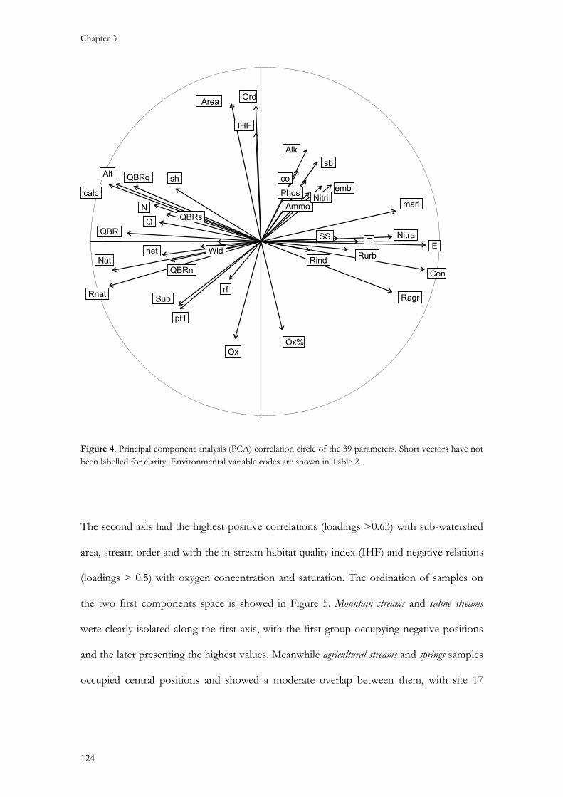
Chapter 3
124
Figure 4. Principal component analysis (PCA) correlation circle of the 39 parameters. Short vectors have not been labelled for clarity. Environmental variable codes are shown in Table 2.
The second axis had the highest positive correlations (loadings >0.63) with sub-watershed
area, stream order and with the in-stream habitat quality index (IHF) and negative relations
(loadings > 0.5) with oxygen concentration and saturation. The ordination of samples on
the two first components space is showed in Figure 5. Mountain streams and saline streams
were clearly isolated along the first axis, with the first group occupying negative positions
and the later presenting the highest values. Meanwhile agricultural streams and springs samples
occupied central positions and showed a moderate overlap between them, with site 17
SS
AmmoNitri
Nitra
Phos
Alk
Q
OxOx%
pH
T
Con
E
N
calcmarl
Alt
Wid
Sub
Ord
RurbRind
RagrRnat
Area
Nat
IHF
emb
rf
sb
sh
het
co
QBR
QBRs
QBRq
QBRn

Chapter 3
125
samples grouped with the agricultural streams samples. The second component (only 11 % of
absorbed variance) of the PCA does not discriminate stream types, but it separated sites
Figure 5. PCA plot of the samples, grouped by stream types. Lines link samples to their stream types. Labels are plotted on the average positions occupied by the sites from each group.
within stream types (all but saline streams) mainly on the base of stream size (catchment
area, order). Site 4, a karstic spring-fed stream in the mountain streams group occupied the
Springs
Agricultural streams
Mountainstreams
Saline streams
Springs
Agricultural streams
Mountainstreams
Saline streams

Chapter 3
126
most negative values, followed by site 11 and site 13, from springs and agricultural streams
respectively, and saline streams.
3.1.3. Biological traits table (Qb)
The two first axes of the fuzzy correspondence analysis (FCA) on the biological traits-taxa
matrix accounted for 20.71 % of the total variance (total inertia 2.05, Table 3). The first
axis was mainly correlated with feeding habits and type of food and to a lesser degree with
maximal size, life cycle duration and reproductive strategy, although for the first and latter
the highest correlation was with axis two (Figure 6). The second axis was principally
correlated with the type of respiration, the reproductive strategy and the maximal size.
Modalities of the variables feeding habits were also separated on this axis but not as much
as on the first axis (Figure 6). The third axis (8.7 % of variance) was positively correlated
with reproduction and feeding habits, so that it did not add new information to the analysis
so that it was not considered further.
The plot of taxa (grouped as orders) on the two first FCA axes is shown in Figure 7. Long-
lived taxa with higher maximal sizes occupied positive values along both axes. They were
predators feeding on living macroinvertebrates, laying isolated eggs (both free and
cemented) and with gill respiration. Invertebrates in this group comprised Odonata, the
Megaloptera Sialis sp., some taxa in Plecoptera (Perla sp. and Dinocras sp.), Trichoptera
(Rhyacophilidae), Ephemeroptera (Ephemera sp.) or crustaceans (crayfish) as well as
Tricladida and Hirudinea. On the contrary, the upper-left quadrant (negative values on F1
and positive on F2) was mainly occupied by medium sized filterers and deposit-feeders
feeding on detritus, fines and microorganisms. They were short-lived taxa (1 year or less),
and the typical reproduction was sexual with free clutches. The respiration mechanisms
were tegument or gills. Most of the Ephemeroptera, Trichoptera, Diptera and Plecoptera

Chapter 3
127
d = 1
Maximal size
<0.25 25–0.5
0.5–1 1–2
2–4
4–8
>8
d = 1
Life cycle duration
1 >1
d = 1
Potential No. rep. cycles per year
<1
1 >1
d = 1
Aquatic stages
egg
lar pu
ad
d = 1
Reproduction
ov
efr ec
cfx
cfr
cv ct
asx
d = 1
Dissemination
aqp
aqa
aep aea
d = 1
Resistance form
egst
coc
cdes
dia no
d = 1
Food
s-m fde cde
lmph
lMph sdan
lminv
lMinv ver
d = 1
Feeding habits
ab depf
shr
filt
pier
pred
par
d = 1
Respiration
teg gi
plst spi
d = 1
Locomotion and substrate relation
fli sswim
fswim
crawbur
int tat pat
scr
0.30
0.38
0.27
0.00
0.22
0.19
0.14
0.07
0.26
0.40
0.11
0.05
0.04
0.14
0.40
0.08
0.43
0.30
0.09
0.45
0.16
0.17
d = 1
Maximal size
<0.25 25–0.5
0.5–1 1–2
2–4
4–8
>8
d = 1
Life cycle duration
1 >1
d = 1
Potential No. rep. cycles per year
<1
1 >1
d = 1
Aquatic stages
egg
lar pu
ad
d = 1
Reproduction
ov
efr ec
cfx
cfr
cv ct
asx
d = 1
Dissemination
aqp
aqa
aep aea
d = 1
Resistance form
egst
coc
cdes
dia no
d = 1
Food
s-m fde cde
lmph
lMph sdan
lminv
lMinv ver
d = 1
Feeding habits
ab depf
shr
filt
pier
pred
par
d = 1
Respiration
teg gi
plst spi
d = 1
Locomotion and substrate relation
fli sswim
fswim
crawbur
int tat pat
scr
0.30
0.38
0.27
0.00
0.22
0.19
0.14
0.07
0.26
0.40
0.11
0.05
0.04
0.14
0.40
0.08
0.43
0.30
0.09
0.45
0.16
0.17
Figure 6. Distribution of modalities (white labels) of the biological traits on the F1-F2 factorial plane of the fuzzy correspondence analysis (FCA). Each modality label was positioned at the weighted average of the taxon positions (solid squares, compare Fig. 7) representing this modality. Numbers indicated the correlation ratios with axis F1 (horizontal numbers) and F2 (vertical numbers). Some labels have been moved for clarity and their actual position is indicated by arrows. Ordination plot scale (i.e. the longitude of the main divisions, “d”) is indicated. Codes used for trait modalities are shown in Table 1a.

Chapter 3
128
Figure 7. Distribution of macroinvertebrate taxonomic units on the F1-F2 factorial plane of the fuzzy correspondence analysis on biological traits. Taxonomic units (white square labels) were positioned at the weighted average of their taxa (solid circles); lines link taxa to their systematic units. Those taxa having extreme scores relative to their groups are indicated (dotted line square labels). For taxa codes, see Appendix 1. Ordination plot scale (i.e. the longitude of the main divisions, “d”) is indicated.
formed the bulge of this group, with some bivalves as Pisidium sp. The negative F2 values
were typical of smaller taxa with short and long live spans. The normal reproductive
strategies were sexual with fixed terrestrial and endophytic clutches. Scrapers feeding on
living macrophytes and piercers of small invertebrates or vertebrates were the main
functional feeding guilds. Respiration was mainly by plastron or aerial by spiracles.
d = 0.5
Cole
Het
Ephe Odo
Tric
Plec
Mega
Dip
Crus
Mol
Tricl Hirud
Olig
Dyti
Helop
HydraHydrch
Hydrph
Mela
Ocht
Micrn
Micrv
Nepa
Plea
Siga
Ephe
Aesh
Boye
Orthe
Cord
Gomp
Onyc
ChimLype
Agap
Stac
PerlDino
Chirm
Tanyt
Tipu
Dicra
Athe
Taba
Pisi
Bero
Ilyb
Isch Platy
pRhy
Rhy
Dixe
Athry
Ephy
Chry
Aust
Proc
Plan
Odo
Oxye Orthot
Chapter 3
129
Coleoptera and Heteroptera mainly composed this group, along with some taxa in
Mollusca and Diptera.
3.1.4. Ecological traits table (Qe)
The two first axes of the fuzzy correspondence analysis (FCA) on the ecological traits-taxa
matrix accounted for 43.2 % of the total variance (total inertia 0.65, Table 3). The first axis
(27.9 %) was mainly correlated with current velocity preference, transversal and
longitudinal distribution and to a lesser degree with productivity preference, saprobity or
microhabitat preferendum (Figure 8). The second axis (15.3 %) was principally correlated
with temperature preference and more weakly with longitudinal distribution but not as
much as on the first axis (Figure 8). The third axis (7.5 % of variance) was also positively
correlated with temperature, not adding new information to the analysis so that it was not
considered further.
The plots of taxa (classified by taxonomic groups) on the two first FCA axes are shown in
Figure 9. Taxa preferring moderate to fast current velocities, mainly inhabiting the main
channel or the banks of rithral and crenal sections of streams, had the highest scores on the
first ordination axis. They were xenosaprobic and oligosaprobic taxa showing preference
for oligotrophic or mesotrophic waters. Microhabitat preferences were mainly rocky
substrates, gravel as well as twigs and roots or sand. The plecopterans, a number of
mayflies (e.g. Epeorus sp., Rhitrogena sp.) and caddisflies (e.g. Pararhyacophila sp., Chimarra sp.)
along with some Elmidae, the European crayfish Austropotamobius sp. or some dipterans
such as Dixa sp. or the Empididae showed the highest scores (Figure 9).

Chapter 3
130
d = 1
Temperature
Co
Wa
Eur
d = 1
pH
<4 4-4.5 4.5-5 5-5.5 5.5-6 >6
d = 1
Productivity
OliMes Eu
d = 1
Saprobity
XenOlig
ß-mes
α-mes
Poly
d = 1
Salinity
FreshBrack
d = 1
Altitude
Low
Pied
Alp
d = 1
Longitudinal distribution
Cre
Epir
Metar
Hypor
EpipMetap
Hypop
Out
d = 1
Transversal - Vertical distribution
Chan
BankPond
Marsh
Temp
LakSubt
d = 1
Microhabitat
Roc
GraSand
Silt
Maph
Miph
Twig
Litt
Mud Rock
d = 1
Current velocity
StagSlow
Mod
Fast
0.09
0.49
0.00
0.02
0.23
0.02
0.18
0.03
0.07
0.01
0.07
0.06
0.27
0.21
0.33
0.05
0.16
0.01
0.41
0.10
d = 1
Temperature
Co
Wa
Eur
d = 1
pH
<4 4-4.5 4.5-5 5-5.5 5.5-6 >6
d = 1
Productivity
OliMes Eu
d = 1
Saprobity
XenOlig
ß-mes
α-mes
Poly
d = 1
Salinity
FreshBrack
d = 1
Altitude
Low
Pied
Alp
d = 1
Longitudinal distribution
Cre
Epir
Metar
Hypor
EpipMetap
Hypop
Out
d = 1
Transversal - Vertical distribution
Chan
BankPond
Marsh
Temp
LakSubt
d = 1
Microhabitat
Roc
GraSand
Silt
Maph
Miph
Twig
Litt
Mud Rock
d = 1
Current velocity
StagSlow
Mod
Fast
0.09
0.49
0.00
0.02
0.23
0.02
0.18
0.03
0.07
0.01
0.07
0.06
0.27
0.21
0.33
0.05
0.16
0.01
0.41
0.10
Figure 8. Distribution of modalities (white labels) of the ecological traits on the F1-F2 factorial plane of the fuzzy correspondence analysis (FCA). Each modality label was positioned at the weighted average of the taxon positions (solid squares, compare Fig. 9) representing this modality. Numbers indicated the correlation ratios with axis F1 (horizontal numbers) and F2 (vertical numbers). Some text labels have been moved for clarity and their actual position is indicated by arrows. Ordination plot scale (i.e. the longitude of the main divisions, “d”) is indicated. Codes used for trait modalities are shown in Table 1b.
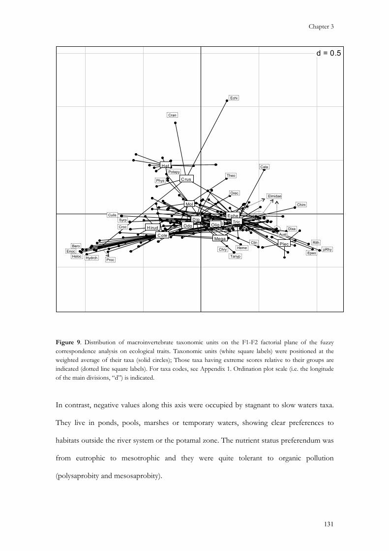
Chapter 3
131
Figure 9. Distribution of macroinvertebrate taxonomic units on the F1-F2 factorial plane of the fuzzy correspondence analysis on ecological traits. Taxonomic units (white square labels) were positioned at the weighted average of their taxa (solid circles); Those taxa having extreme scores relative to their groups are indicated (dotted line square labels). For taxa codes, see Appendix 1. Ordination plot scale (i.e. the longitude of the main divisions, “d”) is indicated.
In contrast, negative values along this axis were occupied by stagnant to slow waters taxa.
They live in ponds, pools, marshes or temporary waters, showing clear preferences to
habitats outside the river system or the potamal zone. The nutrient status preferendum was
from eutrophic to mesotrophic and they were quite tolerant to organic pollution
(polysaprobity and mesosaprobity).
d = 0.5
Cole
Het
Ephe
Odo Tric
Plec Mega
D ip
Crus
Mol
Tric l H irud Olig
Cala
Theo
Chim
Rith
EpeopRhy
Dixa
OrecElmidae
Tanyp
Heme Clin
Chry
Aust
Hydrch
EnocHeloc
Bero
Croc
CulisSyrp
Proc
Phys
Potapy
Echi
Cran

Chapter 3
132
Preferred microhabitats counted microphytes, mud, litter and macrophytes. A number of
water beetles were located in this zone, mainly hydrophilids (as Enochrus sp., Berosus sp. or
Helochares sp.) and some Dytiscidae. Some dipterans as Culiseta sp. or the Syrphidae, the
introduced crayfish Procambarus sp. and the Anisoptera Crocothemis sp. presented low scores
too (Figure 9).
Warm waters taxa preferring lower stream reaches (the hypopotamon and metapotamon)
occupied the highest positive values along the second ordination axis and moderately
negative values along axis 1. They were the Heteroptera along with two crustaceans
(Echinogammarus sp. and Crangonyx sp.) and two gastropods (Physella sp. and Potamopyrgus sp.)
(Figure 9).
3.2. RLQb: Joint analysis of biological traits, environmental variables, and
taxonomic composition
The first two axes of the RLQb analysis extracted 78.3 % and 8.9 % respectively, of the
total variance of the matrix that crosses the site environmental characteristics and the
biological traits of the genera (Table 4). The 1000 random permutations test resulted highly
significant (estimated P = 0.001) which is interpreted as a strong evidence of the link
between biological traits and environmental attributes. The first RLQb axis accounted for
98.5 % of the potential variability for the first axis in the separated PCA of the
environmental variables (i.e., the ratio between the variance of the habitat characteristics
accounted for in RLQb (11.6) and that of the separate analysis (11.8) is 0.985, see Table 3
and Table 4). Similarly, it took into account 51.9 % of the potential variability for the first
axis in the separate analysis of the biological traits. The two new sets of sites and taxa
scores had a correlation of 0.40 along the first RLQb axis (Table 4), a value to be compared
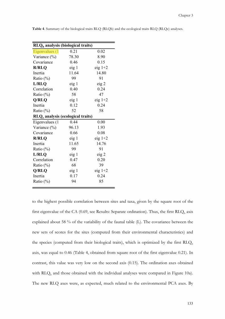
Chapter 3
133
Table 4. Summary of the biological traits RLQ (RLQb) and the ecological traits RLQ (RLQe) analyses.
RLQb analysis (biological traits)Eigenvalues (1 0.21 0.02Variance (%) 78.30 8.90Covariance 0.46 0.15R/RLQ eig 1 eig 1+2Inertia 11.64 14.80Ratio (%) 99 91L/RLQ eig 1 eig 2Correlation 0.40 0.24Ratio (%) 58 47Q/RLQ eig 1 eig 1+2Inertia 0.12 0.24Ratio (%) 52 58RLQe analysis (ecological traits)Eigenvalues (1 0.44 0.00Variance (%) 96.13 1.93Covariance 0.66 0.08R/RLQ eig 1 eig 1+2Inertia 11.65 14.76Ratio (%) 99 91L/RLQ eig 1 eig 2Correlation 0.47 0.20Ratio (%) 68 39Q/RLQ eig 1 eig 1+2Inertia 0.17 0.24Ratio (%) 94 85
to the highest possible correlation between sites and taxa, given by the square root of the
first eigenvalue of the CA (0.69, see Results: Separate ordination). Thus, the first RLQb axis
explained about 58 % of the variability of the faunal table (L). The covariance between the
new sets of scores for the sites (computed from their environmental characteristics) and
the species (computed from their biological traits), which is optimized by the first RLQb
axis, was equal to 0.46 (Table 4, obtained from square root of the first eigenvalue 0.21). In
contrast, this value was very low on the second axis (0.15). The ordination axes obtained
with RLQb and those obtained with the individual analyses were compared in Figure 10a).
The new RLQ axes were, as expected, much related to the environmental PCA axes. By

Chapter 3
134
contrast, the RLQb axes did not stand for the information given by the three first axes of
the separate analysis of the biological traits, but a combination of them (Figure 10a).
Because of the low variance explained by the second RLQb axis, this was not further
considered.
Correlation ratios obtained for the biological traits and the first RLQb axis are presented in
Table 5. Maximal size, reproductive strategy, respiration and resistance form, were the main
attributes explaining the observed biological variability linked to the environmental trends.
Environmental variables loadings on the first RLQb axis are presented in Table 2. Nitrate,
water temperature, electric conductivity, eastern longitude and agricultural use were
negatively correlated with the first RLQb axis, while calcareous geology, altitude, riparian
quality, natural land use and northern latitude were the main positive correlates.
Taxa, biological trait modalities and sampling sites, as well as environmental variables
scores on the first RLQb axis were plotted to summarize the results derived from the
analysis (Figure 11). To facilitate the interpretation of the graph, taxa scores were plotted
according to higher taxonomic groups (usually order) and environmental factors were
grouped in physicochemical, in-stream habitat, riparian forest, geo-morphological and land
use variables (Table 2). Samples were also classified by stream types. Looking at the
positive extreme of the RLQ axis gradient (Figure 11), it is apparent that sites within
forested and/or naturalized catchments tend to have well preserved riparian forests (QBR,
QBRq), high riffle frequency, rocky substrates, shaded channels and heterogeneity elements

Chapter 3
135
Figure 10. Projection of the axes of each separate analysis on the first two RLQ ordination axes. The graphs on a) correspond to the joint analysis of the environmental data (left, R axes) and the biological traits (right, Q axes). The graphs on b) correspond to the joint analysis of the environmental data (left) and the ecological traits (right). Numbers refer to the number of axes selected in each of the separate analysis (see Results).
Ax1
Ax2
R axes projections on RLQ-biotraits axes
Ax1
Ax2
Ax3
Q axes projections on RLQ-biotraits axes
Ax1
Ax2
R axes projections on RLQ-ecotraits axes
Ax1
Ax2
Q axes projections on RLQ-ecotraits axes
a)
b)

Chapter 3
136
Table 5. Biological and ecological traits correlation ratios with their respective first RLQ axes.
Ecological trait Correlation RatioTemperature 0.54pH 0.13Productivity 0.47Saprobity 0.36Salinity 0.21Altitude 0.31Longitudinal distribution 0.44Transversal and vertical distribution 0.48Microhabitat 0.32Current velocity 0.55
Biological trait Correlation RatioMaximal size 0.81Life cycle duration 0.61Potential no. reproductive cycles per year 0.61Aquatic stages 0.20Reproduction 0.76Dissemination 0.25Resistance form 0.67Food 0.28Feeding habits 0.54Respiration 0.74Locomotion and substrate relation 0.46
as twigs, roots or debris dams, and a variety of velocity/depth regimes. They are located at
high elevations in limestone geology catchments of the humid north western part of the
basin, being hard-water sites with relatively high discharge and well oxygenated waters.
Samples on this position matched the mountain streams type sites (Figure 11). Distinctive
biological traits (Figure 11) characterizing the faunal assemblages are: big sizes (2 to 4 cm
and 4 to 8 cm classes) and semivoltinism; sexual reproduction laying cemented eggs as
reproductive strategy; eggs and statoblasts as resistant stages; relative tendency to passive
and active aquatic dispersion; plant debris or fine sediment and microorganisms
consumers, with scrapers and filters as the main functional feeding guilds; tegument
respiration; and finally permanent attachment, burrowing or crawling as the principal
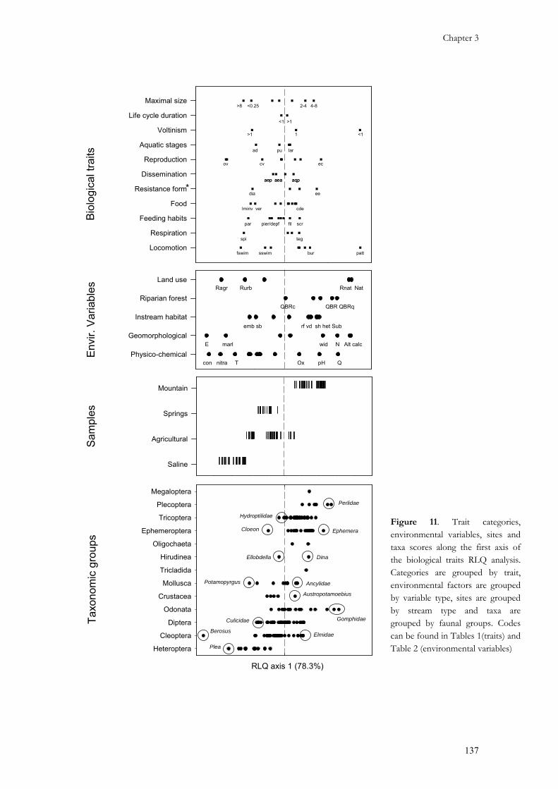
Chapter 3
137
Maximal size
Life cycle duration
Voltinism
Aquatic stages
Reproduction
Dissemination
Resistance form
Food
Feeding habits
Respiration
Locomotion
Env
ir. V
aria
bles
Physico-chemical
Geomorphological
Instream habitat
Riparian forest
Land use
Sam
ples
Saline
Agricultural
Springs
Mountain
RLQ axis 1 (78.3%)
Heteroptera
Cleoptera
Diptera
Odonata
Crustacea
Mollusca
Tricladida
Hirudinea
Oligochaeta
Ephemeroptera
Tricoptera
Plecoptera
Megaloptera
Bio
logi
cal t
raits
Taxo
nom
ic g
roup
s>8 <0.25 4-82-4
>1 1 <1
ad pu lar
ov cv ec
aep aea aqp
*dia ee
lminv ver cde
par pier/depf fil scr
spi teg
fswim sswim bur patt
Ragr Rurb Rnat Nat
QBRc QBR QBRq
emb sb rf vd sh het Sub
E marl wid N Alt calc
con nitra T Ox pH Q
Berosus
Plea
Elmidae
Culicidae Gomphidae
Austropotamoebius
AncylidaePotamopyrgus
DinaEllobdella
EphemeraCloeon
Hydroptilidae
Perlidae
<1 >1
Maximal size
Life cycle duration
Voltinism
Aquatic stages
Reproduction
Dissemination
Resistance form
Food
Feeding habits
Respiration
Locomotion
Env
ir. V
aria
bles
Physico-chemical
Geomorphological
Instream habitat
Riparian forest
Land use
Sam
ples
Saline
Agricultural
Springs
Mountain
RLQ axis 1 (78.3%)
Heteroptera
Cleoptera
Diptera
Odonata
Crustacea
Mollusca
Tricladida
Hirudinea
Oligochaeta
Ephemeroptera
Tricoptera
Plecoptera
Megaloptera
Bio
logi
cal t
raits
Taxo
nom
ic g
roup
s>8 <0.25 4-82-4
>1 1 <1
ad pu lar
ov cv ec
aep aea aqpaep aea aqp
*dia ee
lminv ver cde
par pier/depf fil scr
spi teg
fswim sswim bur patt
Ragr Rurb Rnat Nat
QBRc QBR QBRq
emb sb rf vd sh het Sub
E marl wid N Alt calc
con nitra T Ox pH Q
Berosus
Plea
Elmidae
Culicidae Gomphidae
Austropotamoebius
AncylidaePotamopyrgus
DinaEllobdella
EphemeraCloeon
Hydroptilidae
Perlidae
<1 >1
Figure 11. Trait categories, environmental variables, sites and taxa scores along the first axis of the biological traits RLQ analysis. Categories are grouped by trait, environmental factors are grouped by variable type, sites are grouped by stream type and taxa are grouped by faunal groups. Codes can be found in Tables 1(traits) and Table 2 (environmental variables)

Chapter 3
138
locomotion and substrate relationships (Figure 11). All the Plecoptera and most of
Ephemeroptera and Trichoptera (EPT taxa) occupied this right side of the axis (Figure 11),
along with Ancylus sp., Ferrisia sp., Austropotamobius sp., anisopterans as Gomphidae and
Cordulegaster sp., and most Elmidae. Contrastingly, sites located in the semi-arid south-
eastern part of the study area are characterized mainly by agricultural and land-uses and
also included the most urbanized catchments. Dominant geologies are marls with
quaternary alluvial deposits and elevation is low at most of sampling sites. Riparian forests
and stream channel morphology, as evaluated with the QBR index and its sub-metrics, are
not of good quality (presence of introduced species and human alterations in vegetation
and/or channel form). Among in-stream habitat variables, high substrate embeddedness,
visually estimated as the degree of interstitial filling of the substratum by fine particles and
substrate size heterogeneity were the principal differential features. Physico-chemical
attributes included high conductivities and nitrate content, high temperature and high
suspended solids content. Samples from sites classified as saline streams matched this
environmental features in the graph, being located at the negative extreme of the gradient.
Common biological traits exhibited by the macroinvertebrate communities inhabiting these
systems were: the highest as well as the smallest sizes (<0.25 and >8 cm), polyvoltinism,
aquatic adults, ovoviparity and endophytic clutches; relative affinity for aerial dispersion,
cells against desiccation and diapause or dormancy as resistance strategies, living
microinvertebrates or vertebrates as the main food sources, parasitic or predatory (piercers)
feeding behaviour, aerial respiration through spiracles and swimming locomotion, (both
water column and surface swimmers). The majority of the Heteroptera, the hydrophilid
Berosus sp. (and to a lesser degree Haliplus sp. or Ilybius sp.) some dipterans in Culicidae and
snails as Potamopyrgus sp. dominated the negative side of the RLQb axis. Among the
Ephemeroptera, the genus with the lowest score was Cloeon sp.
Chapter 3
139
3.3. RLQe: Joint analysis of ecological traits, environmental variables, and
taxonomic composition
The first two axes of the RLQe analysis extracted 96.1 % and 1.9 % respectively, of the
total variance of the matrix that crosses the site environmental characteristics and the
ecological traits of the genera (Table 4). Again, the 1000 random permutations resulted in a
highly significant link between environmental variables and ecological traits through the
species abundance (estimated P = 0.001). Similarly as what occurred analyzing biological
traits, the first axis of the RLQe analysis accounted for 98.6 % of the potential variability
for the first axis in the separated PCA of the environmental variables of the habitats (i.e.,
the ratio between the variance of the habitat characteristics accounted for in RLQe (11.7)
and that of the separate analysis (11.8) is 0.986, see Tables 3 and 4). However, the
proportion of the potential variability for the first axis in the separate analysis of the
ecological traits (94 %) was much higher than the one obtained using biological traits (52
%). The two new sets of sites and taxa scores had a correlation of 0.47 along the first RLQe
axis (Table 4), which again has to be compared to the square root of the first eigenvalue of
the CA of the taxonomic abundance table (0.69, see Results: Separate ordinations). Thus,
the first RLQe axis explained about 68 % of the variability of the faunal table (L) obtained
by CA. The covariance between the new sets of scores for the sites (computed from their
environmental characteristics) and the genera (computed from their ecological traits),
which is optimized by the first RLQ axis, was equal to 0.66 (Table 4, obtained from square
root of the first eigenvalue 0.44). In contrast, this value was again very low on the second
axis (0.09). The ordination axes obtained with RLQe and those obtained with the separate
analysis of the individual tables were compared in Figure 10b). The structure of the
environmental matrix described by the RLQe axes was, as expected, very close to that of
the separate PCA. In this occasion, the RLQe axes also represented (almost directly) the
information given by the two first axes of the separate analysis of the ecological traits. This
Chapter 3
140
result was somehow expected, as our ecological traits (optima for various environmental
variables) are directly related to the measured habitat factors, while more subtle
relationships were assumed for life-history or behaviour traits. As was the case for the
biological traits analysis, the second RLQe axis was not considered further due to the very
low variance explained (1.9 %).
Correlation ratios obtained for the ecological traits and the first RLQe axis are presented in
Table 5. Temperature, productivity, longitudinal and transversal distribution as well as
current velocity preferendum were the main traits explaining the observed ecological
variability linked to the environmental trends.
A similar uni-dimensional plot was constructed where taxa, ecological trait modalities and
samples scores, as well as environmental variables loadings on the first RLQe axis were
plotted to summarize the results (Figure 12). The loadings of environmental variables as
well as sites and taxa scores were very similar to those obtained using biological traits,
although with opposite sign (Table 2) The negative correlation between the 209 genera
scores on the two RLQ axes (RLQb-1 and RLQe-1) was equal to -0.67, while between the
104 site scores and the 39 environmental variables loadings was equal to -0.99 in both
cases. For clarity, we change the sign of the axis in this plot, to resemble that obtained for
the biological traits analysis. Thus, the same environmental interpretation of the RLQb axis
is valid in this case. According to the ecological preferences of the macroinvertebrate fauna,
the positive extreme of the RLQe axis was characterized by cold-water taxa, preferring
oligotrophic systems and with very low tolerance values to organic pollution (xenosaprobic
and oligosaprobic taxa). They tended to prefer high altitude reaches in the epirithral and
metarithral sections, where they usually occupy the main channel. Preferred habitats were
rock, gravel or sand substrates with moderate to fast current velocity.

Chapter 3
141
Temperature
pH
Productivity
Saprobity
Salinity
Altitude
Longitudinal distribution
Transv-vertical distribution
Microhabitat
Current velocity
Envi
r. Va
riabl
es
Land use
Riparian forest
Instream habitat
Geomorphological
Physico-chemical
Sam
ples
Saline
Agricultural
Springs
Mountain
RLQ axis 1 (96.1%)
Heteroptera
Cleoptera
Diptera
Odonata
Crustacea
Mollusca
Tricladida
Hirudinea
Oligochaeta
Ephemeroptera
Tricoptera
Plecoptera
Megaloptera
Ecol
ogic
al tr
aits
Taxo
nom
ic g
roup
sWa Co
Eu Oli
<4
Poly a-mes Olig Xen
Brack Fresh
AlpLow
Out Hypop Metap Metar Epir
Marsh Pond Temp Bank Subt Chan
Miph Mud Litt Sand Gra Roc
Stag Slow Mod Fast
Enochrus, Helochares, Berosus
Plea, Anisops
Elmidae, Pomatinus
Dixa
Cordulegaster, Boyeria
Procambarus Austropotamoebius
AncylusPotamopyrgus
Epeorus, Rhytrogena
Cloeon
Pararhyacophila
QBRc QBR QBRq
E marl w N Alt /calc
sb inc het Sub/sh
Con Nitra T Oxy pH Q
Ragr Rurb Nat / Rnat
Velia
Syrphidae, Culicidae
Crocothemis
Orthotrichia, Cyrnus
Temperature
pH
Productivity
Saprobity
Salinity
Altitude
Longitudinal distribution
Transv-vertical distribution
Microhabitat
Current velocity
Envi
r. Va
riabl
es
Land use
Riparian forest
Instream habitat
Geomorphological
Physico-chemical
Sam
ples
Saline
Agricultural
Springs
Mountain
RLQ axis 1 (96.1%)
Heteroptera
Cleoptera
Diptera
Odonata
Crustacea
Mollusca
Tricladida
Hirudinea
Oligochaeta
Ephemeroptera
Tricoptera
Plecoptera
Megaloptera
Ecol
ogic
al tr
aits
Taxo
nom
ic g
roup
sWa Co
Eu Oli
<4
Poly a-mes Olig Xen
Brack Fresh
AlpLow AlpLow
Out Hypop Metap Metar Epir
Marsh Pond Temp Bank Subt Chan
Miph Mud Litt Sand Gra Roc
Stag Slow Mod Fast
Enochrus, Helochares, Berosus
Plea, Anisops
Elmidae, Pomatinus
Dixa
Cordulegaster, Boyeria
Procambarus Austropotamoebius
AncylusPotamopyrgus
Epeorus, Rhytrogena
Cloeon
Pararhyacophila
QBRc QBR QBRq
E marl w N Alt /calc
sb inc het Sub/sh
Con Nitra T Oxy pH Q
Ragr Rurb Nat / Rnat
Velia
Syrphidae, Culicidae
Crocothemis
Orthotrichia, Cyrnus Figure 12. Trait categories,
environmental variables, sites and taxa scores along the first axis of the ecological traits RLQ analysis. Categories are grouped by trait, environmental factors are grouped by variable type, sites are grouped by stream type and taxa are grouped by faunal groups. Codes can be found in Tables 1(traits) and Table 2 (environmental variables)

Chapter 3
142
Plecoptera and most of Ephemeroptera and Trichoptera occupied this right side of the
axis, along with Ancylus sp., Austropotamobius sp., anisopterans as Cordulegaster sp. or Boyeria
sp., the dipteran Dixa sp., and water beetles such as Elmidae, Pomatinus sp. (Dryopidae) or
Oreodytes sp. (Dytiscidae). Contrasting ecological characteristic matched the negative part of
gradient: common biological traits included high temperature preference, tolerance to low
pH and high organic pollution or preference for saline waters and eutrophic systems. They
are taxa usually found in potamal sections of streams or even outside of the river system,
where they tend to live in marshes, ponds and pools or temporary waters. Preferred
microhabitats were microphites, mood or litter substrates and stagnant waters. A number
of taxa in Heteroptera, many Hydrophilidae as Enochrus sp., Helochares sp., Berosus sp., or
Paracymus sp., some dipterans as all Culicidae and Syrphidae, dragonflies and damselflies
(Sympetrum sp. or Ischnura sp.), crustaceans as Procambarus sp. and snails as Potamopyrgus sp.
dominated the left side of the axis. Among the Ephemeroptera, the genus with the lowest
score was again Cloeon sp.

Chapter 3
143
4. Discussion
4.1. Environmental factors driving community characteristics Results have shown that a variety of environmental factors was related to the observed
community structure and biological/ecological attributes. The most influential variables,
i.e., those that showed the highest or lowest values along both biological and ecological
RLQ axes were agricultural and natural/forest, riparian forest quality, surficial geology and
altitude. There was also a strong spatial influence, with geographical coordinates (and
specially longitude) as correlates. Electric conductivity, nitrate, water temperature and
discharge also exerted major influences. Among the in-stream habitat variables, those
related to substrate size and heterogeneity were the most influential, but to a lesser degree
in comparison with the other variables.
Contrastingly, among the variables identified as not being very relevant (those positioned
near the centre of the axis) were riparian cover percentage, the in-stream habitat index, the
macrophyte cover, the stream order, the catchment area or the oxygen contents
When viewed across relatively large spatial scales, much variation in species distributions
can be attributed to patterns of variation within the landscape. Large-scale landscape
attributes such as land use, surficial geology, elevation, and hydrology were found by
Richards et al. (1996) to have the greatest influence on macroinvertebrate assemblages.
However, Richards et al., 1997 found that reach-scale physical features were best related to
certain life history and behavioural attributes of macroinvertebrates than catchment-scale
variables, suggesting that species traits exhibit strong relationships to local environmental
conditions. Our results suggest that a variety of factors acting at different scales and
hierarchically organized (for example, agricultural use and percentage of marls are dictating
Chapter 3
144
the conductivity and nitrate content and also influencing the riparian habitat or the
substrate) controls the functional organization of communities at our scale of study.
4.2. Taxa traits and environmental attributes RLQ analysis relates species traits directly to changes in environmental attributes. Thus,
major natural environmental variables and anthropogenic alterations important to stream
communities were revealed, as well as the biological and ecological traits responding to
these properties. We found a highly significant relationship between both biological and
ecological traits, expressed by sets of life-history/behavioural/physiological characters and
environmental preferences, and the environmental features of the habitats, as measured by
the main underlying environmental gradient. In both RLQ analyses, the first ordination
axes accounted for very large fractions of the explained variance, indicating the existence of
a strong environmental gradient structuring the characteristics of the sites and taxa. This
was extremely accentuated in the case of the ecological traits analysis (96 % of variance
absorbed by the first axis). The ordination of sites along this axis closely matched our a-
priori biotic classification of stream types. Saline streams were located in the left extreme of
the gradient, while agricultural streams and springs occupied more central (but still negative)
positions (compare Figures 11 and 12). The nature of the environmental factors that
dominate this part of the gradient (disturbed land-use, no riparian forests, south-eastern
gradient, high nutrient loadings, marly geology, high conductivities, etc.) would indicate an
area with very high anthropogenic pressure and so that very threatened ecosystems
(Gómez et al., 2005). At the same time, it would reflect a natural disturbance regime typical
of semi-arid streams, characterized by extremes of flood and drought, these events being
the most important natural disturbance agents in these ecosystems (Fisher & Grimm,
1991). Both factors, along with a high tolerance to salinity control and shape the structure

Chapter 3
145
and functioning of the whole aquatic ecosystem and influence the characteristics of the
biota of these characteristics streams locally called “ramblas”. (Gómez et al., 2005). This
region of the gradient matched some of the biological traits so cited in the literature as
providing resilience and/or resistance to disturbances, i.e. small sizes and high number of
generations per year (Southwood, 1977, 1988; Townsend and Hildrew, 1994). Other
biological features that remove or reduce the impact of environmental fluctuations were
the presence of adults known to cope with drought episodes by resistant cells (such as the
hydrophilid water beetle Berosus), diapause and dormancy as resistance stages and the laying
of endophytic eggs. The presence of aquatic adults can also provide with colonization
mechanisms after floods or drought disturbances. In this sense, the aquatic adults of
Heteroptera and Coleoptera are among the best cyclic colonizers of ephemeral waters and
exemplify the adaptations for this lifestyle (Ortega et al., 1991; Wissinger, 1997 and
references therein; Velasco et al., 1998; Bilton et al., 2001). The prevalence of ovoviviparity
as reproductive strategy was mainly due to the presence of the introduced freshwater snail
Potamopyrgus antipodarum. This trend have been noted in other works (Doledec et al., 1999;
Usseglio-Polatera and Beisel, 2002), where parental care seemed to be more diverse at
reference sites where four types of egg deposition predominated, while ovoviviparity and
regeneration were more frequent at the frequently disturbed sites. This snail often shows
parthenogenetic reproduction, what could also be taken as a factor conferring resilience in
disturbed habitats.
The dominance of fliers in the more stressed environments could reflect a prevalence of
high immediate dispersal ability to cope with disturbance episodes such as floods and
droughts by behavioural adaptations on a per-event basis (Lytle and Poff, 2004).

Chapter 3
146
Nevertheless, some traits usually predicted in more stable and benign conditions were also
present in this part of the gradient, i.e. biggest sizes and vertebrate predation. Looking back
to the original trait matrix, we observed that the introduced American crayfish Procambarus
clarkii was the taxa responsible of these characters, mainly in the agricultural streams. This
species shows characteristics such as opportunistic omnivorous feeding, resistance to
pollution and extreme environmental conditions, fast growth and high reproduction
potential, it requires productive water systems, etc. which make this species particularly
suitable for invading streams affected by cultural eutrophication (Angeler et al., 2001; Gil-
Sanchez and Alba-Tercedor, 2002)
Contrastingly, the right side of the gradient (Figures 11 and 12) was mainly occupied by
samples from stream sites in semi-pristine conditions, located in the well preserved nature
reserves of the humid north-western upper catchment. They corresponded to the mountain
streams typology. The biological traits highlighted large sizes and less than one reproductive
cycle per year. These features have been commonly treated as indicative of relatively stable
habitats with a disturbance regime characterized by low frequency and intensity and high
predictability (Southwood, 1988; MacArthur and Wilson, 1967; Stearns, 1992; Townsend
and Hildrew, 1994). Other characters such as the production of cemented isolated eggs
could be justified as a lesser investment in parental care in a more stable environment.
Statzner et al. (2001) found that streams having sewage influence had significantly lower
abundances of taxa producing isolated cemented eggs in comparison with reference sites,
although they did not find a mechanistic explanation to this trend.
Statzner et al. (2001) hypothesize that compared to reference conditions, streams affected
by sewage input (i.e. reduced oxygen content of the water) would favour various types of
aerial respiration, and abundant land-use in the catchment (i.e. increased erosion and thus

Chapter 3
147
silting of the interstices in the bottom) would disfavour endobenthics; also, the destruction
of the riparian forest (i.e. reduced CPOM input to the stream) would disfavour feeding on
coarse plant detritus. We found all these trends to occur in our study. The aerial respiration
probably was related to low dissolved oxygen levels on account of a mix of factors, i.e. high
temperatures and low flows, high nutrient contents or high suspended solids. Nevertheless,
oxygen concentrations did not appear to be very relevant in the RLQ analysis, being the
sampled streams well oxygenated in most of cases. Aerial respiration is mainly showed by
Coleoptera, Heteroptera and Diptera, and probably factors other than oxygen could be
favouring this trait in these streams (e.g. temperature and salinity tolerance). We also found
a dominance of filters in the mountain streams, almost certainly as a negative response to
the low flows characterizing semi-arid streams. Organisms with permanent attachment to
the substrate, burrowers and interstitial animals were more abundant in the right part of the
graph, coinciding with the mountain streams. Usseglio-Polatera and Beisel (2002) also found a
similar trend (changes in predominance from swimmer and/or crawler to interstitial or
burrower) in a longitudinal characterization of invertebrate communities along the Meuse
River. They found as well a change in feeding habits (piercer and scraper to filterer or
deposit feeder) that match our results too.
In contrast, the ecological traits featured (from left to right in the RLQe axis) saprobity of
taxa (poly- to xenosaprobic), salinity tolerance (brackish to freshwaters), trophic status
preference (eutrophic to olygotrophic), longitudinal distribution (outside river system to
epi-rithral sections), transversal distribution (from marshes and ponds to main channels),
current velocity (fast to null), and microhabitat (microphytes to rocky substrates) as
‘significant’ factors driving the differential ecological features of communities.

Chapter 3
148
4.3 A “habitat templet” for streams in SE Spain Habitats and species traits can be matched directly, but this match occurs in complicated
ways because species traits are expressed in variable combinations in organisms.
Consequently, one can always find organisms with unexpected trade-offs of traits in a given
habitat that violate the assumptions of the general theoretical model (Williams & Feltmate,
1992; Resh et al., 1994; Townsend & Hildrew, 1994).
The habitat templet originally developed by Greenslade (1983) was applied to lentic waters
in the semi-arid regions in Australia (Williams, 1985). The axes of this templet were the
extent of predictability (i.e. disturbance regime) and the salinity level. Our results appeared
to fit this model, with our RLQ axis being equivalent to the diagonal of the templet (Figure
13). Nevertheless, it is difficult to express the longitudinal axis of the templet in terms of a
single variable (namely salinity) due to the variety of confounding factors that correlates
along the main gradient in our catchment (altitude and climate, geology and land-use, etc.
see Chapter 2). Thus, we opted to call this axis the “adversity axis” (as in the original work
by Greenslade), along which natural stressors (i.e. salinity and temporality) are accentuated
by human pressures (agricultural land-use and its corollaries: organic enrichment, water
diversions and physical channel alterations).
4.4 Biological vs ecological traits We found an almost perfect correlation between the first RLQ axis obtained using
biological traits and the one obtained using the ecological traits, which means that each of
the ecological traits was strongly related to one environmental variable measured (and often
more than one, e.g. the preference for eutrophic waters could be related to nitrate content,
conductivity or agricultural land use) and also that the genus-level ecological information

Chapter 3
149
used from Tachet et al. 2000 reflected in a direct way the measured environmental trends.
This matching can also highlight physiological constraints in distribution patterns (see
Chown & Gaston, 1999). For example, organisms with aerial respiration can tolerate high
Figure 13. Proposed theoretical habitat templet for streams in the study area. The stream types studied are located along an adversity axis and a disturbance axis. The main selection models acting in each region of the templet are also indicated. The main diagonal corresponds to the obtained first RLQ axes.
salinity and organic pollution and show preference to still waters, while organisms that
breathe through tegument show the opposite trends, maybe due to osmotic regulation
constraints.
r - selection
K - selection
A - selectionMountainstreams
Agriculturalstreams
Springs
Salinestreams
Adversity, stress
Disturbance
r - selection
K - selection
A - selectionMountainstreams
Agriculturalstreams
Springs
Salinestreams
Adversity, stress
Disturbance

Chapter 3
150
4.5 Future use of species traits as basis for monitoring human impacts Theory predicts different life-history strategies for different disturbance levels or spatio-
temporal heterogeneity (Poff and Ward 1990; Townsend and Hildrew, 1994), and thus
different life-history traits can also indicate different intensities of human impact (Dolèdec
et al., 1999)
RLQ analysis has been used as an effective tool for identifying species traits that respond to
impacts of land use change on different scales. In the initial stage of a monitoring program,
it is suitable to select indicator species traits directly linked to specific ecological processes
modified by human intervention (Hausner et al., 2003). In regards to human impacts in
streams from the Segura river basin, we found changes in land-use (mainly the agricultural
use, with the alteration of riparian corridors, water diversions and nutrient enrichment) to
have the strongest impact on invertebrate assemblages at the catchment scale.
Nevertheless, the confounding effects of geology, altitude and climate precluded any
selection of traits responding to environmental impacts.
Mediterranean-type streams and specially those in semi-arid regions are particularly
susceptible to water diversion (directly or via groundwater withdrawal) and flow regulation
(Gasith and Resh, 1999). Intensive agriculture has proved to be the more destructive
human activity (and more than traditional fruit cultivation) in riparian communities from
the semi-arid south-east of Spain (Salinas et al. 2000) and the expansion of intensive
irrigation crops in Murcia region the last decades have been documented (Martínez-
Fernández et al., 2000; 2002 Vidal-Abarca et al., 2004). Moreover, in a recent work Ortega
et al. (2004) found that intensive agriculture (expressed as potential nitrogen export) was
the main pressure single predictor affecting the ecological integrity of semi-arid wetlands in
south-east Spain. Nevertheless, its effects in stream macroinvertebrate communities have

Chapter 3
151
not been addressed properly yet, although semi-arid saline “ramblas” of south-eastern
Spain are among the most threatened aquatic ecosystems in Spain and probably in Europe
(Abellán et al. 2005; Sánchez-Fernandez et al., 2004; Gomez et al., 2005). Thus, it would be
desirable to investigate the effects of this land-use change separately, eliminating those
confounding effects as far as possible. Nevertheless, we recognize the difficulty of such a
study in our area, at least at a catchment scale study as this.
5. References Abellán, P. Sánchez-Fernández, D., Velasco, J.; Millán, A. 2005. Assessing conservation priorities for insects: status of water beetles in southeast Spain. Biological Conservation 121: 79–90 Aboal, M., 1989. Epilithic algal communities from River Segura Basin, Southeastern Spain. Archiv für Hydrobiologie 116: 113–124. Angeler D.G., Sánchez-Carrillo, García G., Alvarez-Cobelas M. 2001. The influence of Procambarus clarkii (Cambaridae, Decapoda) on water quality and sediment characteristics in a Spanish floodplain wetland. Hydrobiologia 464: 89–98 Barbaro, L., Corcket, E., Dutoit, T. ; Peltier, J. P. 2000. Réponses fonctionnelles des communautés pelouses calcicoles aux facteurs agro-écologiques dans les Préalpes françaises. Canadian Journal of Botany 78: 1010-1020. Barbour, M.T., J. Gerritsen, B.D. Snyder, J.B. Stribling. 1999. Rapid Bioassessment Protocols for Use in Streams and Wadeable Rivers: Periphyton, Benthic Macroinvertebrates and Fish. Second Edition. EPA 841-B-99-002. U.S. Environmental Protection Agency; Office of Water; Washington, D.C. Bilton D.T., Freeland J.R.; Okamura B. 2001. Dispersal in freshwater invertebrates: mechanisms and consequences. Anuual Review of Ecology and Systematics 32: 159–181. Boyero, L. 2003. Multiscale patterns of spatial variation in stream macroinvertebrate communities. Ecological Research18: 365–379

Chapter 3
152
CEC, 1993. CORINE land cover technical guide, European Union. Directorate-General Environment, Nuclear Safety and Civil Protection. Office for Official Publications of the European Communities, Luxemburg. Chevenet, F., Dolédec, S.; Chessel, D. 1994. A fuzzy coding approach for the analysis of long-term ecological data. Freshwater Biology 31: 295–309. Chown, S.L., Gaston, K.J. 1999. Exploring links between physiology and ecology at macro-scales: the role of respiratory metabolism in insects. Biological Review 74: 87-120. Dolédec S., Chessel D. 1994. Co-inertia analysis: an alternative method for studying species-environment relationships. Freshwater Biology, 31: 277-294. Dolédec, S., Chessel, D., ter Braak, C.J.F.; Champely, S. 1996. Matching species traits to environmental variables: a new three-table ordination method. Environmental and Ecological Statistics 3: 143–166. Dolédec, S., Statzner, B.; Frainay, V. 1998. Accurate description of functional community structure: identifying stream invertebrates to species-level? Journal of the North American Benthological Society 15: 154-155. Doledec S., Statzner B., Bournard M., 1999. Species traits for future biomonitoring across ecoregions: patterns along a human-impacted river. Freshwater Biology 42: 737–758 Fisher, S.G.; N.B. Grimm. 1991. Streams and disturbance : Are cross-ecosystem comparison useful?, pp. 196-221 In J. Cole, S.; Findlay; G. Lovett [eds.]. Comparative analysis of ecosystems: patterns, mechanisms and theories. Springer-Verlag, New York. Gasith, A.; V.H. Resh, 1999. Streams in Mediterranean Regions: Abiotic influences and biotic responses to predictable seasonal events. Anuual Review of Ecology and Systematics, 30: 51-81. Gil-Sanchez, J.M.; Alba-Tercedor, J. 2002. Ecology of native and introduced crayfishes Austropotamobius pallipes and Procambarus clarkii in southern Spain and implications for conservation of native species. Biological Conservation, 105: 75–80. Gómez, R., Hurtado, I., Suárez, M.L.; Vidal-Abarca, M.R. 2005. Ramblas in Southeast Spain: threatened and valuable ecosystems Aquatic Conservation. Marine and Freshwater Ecosystems, (in press) Greenslade, P.J.M. 1983. Adversity selection and the habitat templet. American Naturalist 122: 352-365.

Chapter 3
153
Hausner, V.H., Yoccoz, N.G.; Ims, R.A. 2003. Selecting indicator traits for monitoring land use impacts: birds in northern coastal birch forests. Ecological Applications, 13(4): 999–1012 Hooke, J.M., Mant, J. 2002. Floodwater use and management strategies in valleys of southeast Spain. Land Degradation and Development 13 (2): 165-175 Hynes, H.B.N. 1970. The ecology of stream insects. Annual Review of Entomology, 15: 25-42. Legendre, P., Galzin, R.; HarmelinVivien, M.L. 1997. Relating behaviour to habitat: Solutions to the fourth-corner problem. Ecology 78: 547-562. Lenat, D. R.; Resh, V. H. 2001. Taxonomy and stream ecology—The benefits of genus- and species- level identifications. Journal of the North American Benthological Society 20: 287–298. Lytle, D. A.; N.L.Poff. 2004. Adaptation to natural flow regimes. Trends in Ecology and Evolution 19:94-100. MacArthur, R.H.; Wilson, E.O. 1967. The theory of island biogeography. Princeton University Press, New Jersey. Martinez-Fernandez J, Esteve-Selma M.A, Calvo-Sendin J.F. 2000. Environmental and socioeconomic interactions in the evolution of traditional irrigated lands: a dynamic system model. Human Ecology 28: 279–299. Martínez-Fernández, J., M.A. Esteve Selma (coords.). 2002. Agua, regadío y sostenibilidad en el Sudeste Ibérico. Editorial Bakeaz-Fundación Nueva Cultura del Agua, Bilbao. Mellado, A., Suárez, M.L., Moreno, J.L.; Vidal-Abarca, M.R. 2002. Aquatic macroinvertebrate biodiversity in the Segura River Basin (SE Spain). Verh. Internat. Verein. Limnol. 28: 1157-1162. Minshall, G.W.; Robinson, C.T. 1998. Macroinvertebrate community structure in relation to measures of lotic habitat heterogeneity. Archiv für Hydrobiologie 141: 129-151. Moreno, J.L., Millán, A., Suárez, M.L., Vidal-Abarca, M.R. & Velasco, J. 1997. Aquatic Coleoptera and Heteroptera assemblages from ephemeral coastal streams (“ramblas”) of south-eastern Spain. Archiv für Hydrobiologie 141(1): 93–107. Moreno, J.L., Aboal, M., Vidal-Abarca, M.R.; Suárez, M.L. 2001. Macroalgae and submerged macrophytes from fresh and saline waterbodies of ephemeral streams ("ramblas") in semiarid south-eastern Spain. Marine and Freshwater Research 52: 891-905.

Chapter 3
154
Munne, A., Prat, N., Sola, C., Bonada, N.; Rieradevall, M. 2003. A simple field method for assessing the ecological quality of riparian habitat in rivers and streams. QBR index. Aquatic Conservation: Marine and Freshwater Ecosystems 13: 147–163. National Rivers Authority. 1995. River Habitat Survey: Field Methodology Guidance Manual. NRA. Ortega, M., M.L. Suárez, M.R. Vidal-Abarca, R. Gómez, L. Ramírez-Díaz. 1991. Aspects of postflood recolonization of macroinvertebrates in a “rambla” of south-east Spain (“Rambla del Moro”: Segura River Basin). Verh. Internat. Verein. Limnol. 24: 1994–2001. Ortega, M., Velasco, J., Millán, A., Guerrero, C. 2004. An ecological integrity index for littoral wetlands in agricultural catchments of semiarid Mediterranean regions. Environmental Management 33: 412–430 Pardo, I., Álvarez, M., Casas, J., Moreno, J.L., Vivas, Bonada, N., Alba-Tercedor, J., Jáimez-Cuéllar, P., Moyá, G., Prat, N., Robles, S., Suárez, M.L.; Toro, M.; Vidal-Abarca, M.R. 2002. El hábitat de los ríos mediterráneos. Diseño de un índice de diversidad de hábitat. Limnetica, 21(3-4): 115-133 Poff, N.L. 1992. Why disturbances can be predictable: a perspective on the definition of disturbance in streams. Journal of the North American Benthological Society 11: 86–92. Poff, N.L. 1996. A hydrogeography of unregulated streams in the United States and an examination of scale-dependence in some hydrological descriptors. Freshwater Biology 36: 71–91. Poff, N.L. 1997. Landscape filters and species traits: towards mechanistic understanding and prediction in stream ecology. Journal of the North American Benthological Society 16: 391–409. Poff, N.L.; J.V. Ward. 1990. Physical habitat template of lotic systems: recovery in the context of historical pattern of spatiotemporal heterogeneity. Environmental Management 14: 629–645. R Development Core Team. 2004. R: A language and environment for statistical computing. R Foundation for Statistical Computing, Vienna, Austria. ISBN 3-900051-00-3, URL http://www.R-project.org Resh, V.H.; Hildrew, A.G.; Statzner, B.; Townsend, C.R. 1994. Theorical habitat templets, species traits and species richness: A synthesis of long term ecological research on the Upper Rhône River in the context of concurrently developed ecological theory. Freshwater Biology 31: 539-554.

Chapter 3
155
Resh, V.H., A.V. Brown, A.P. Covich, M.E. Gurtz, H.W. Li, G.W. Minshall, S.R. Reice, A.L. Sheldon, J.B. Wallace; R. Wissmar. 1988. The role of disturbance in stream ecology. Journal of the North American Benthological Society 7: 433–455. Ribera, I., S. Dolédec, I. S. Downie, and G. N. Foster. 2001. Effect of land disturbance and stress on species traits of ground beetle assemblages. Ecology 82:1112–1129. Richards C., Johnson L.B.; Host G.H. 1996. Landscape scale influences on stream habitats and biota. Canadian Journal of Fisheries and Aquatic Sciences, 53 (Suppl. 1): 295–311. Richards, C., Haro R.J., Johnson, L.B., Host, G.E. 1997. Catchment and reach-scale properties as indicators of macroinvertebrate species traits. Freshwater Biology 37: 219–230. Salinas, M.J., G. Blanca; A.T. Romero. 2000. Evaluating riparian vegetation in semi-arid Mediterranean watercourses in the south-easter Iberian Peninsula. Environmental Conservation 27:24-35. Sánchez-Fernández, D., Abellán, P. Velasco, J. and Millán, A. 2004. Selecting areas to protect the biodiversity of aquatic ecosystems in a semiarid Mediterranean region using water beetles. Aquatic Conservation: Marine and Freshwater Ecosystems 14: 465–479 Scarsbrook M.R.; Townsend C.R. 1993. Stream community structure in relation to spatial and temporal variation: a habitat templet study of two contrasting New Zealand streams. Freshwater Biology, 29: 395–410. Sedell, J.R., Reeves, G.H., Hauer, F.R., Stanford, J.A.; Hawkins, C.P. 1990. Role of refugia in recovery from disturbances: modern fragmented and disconnected river systems. Environmental Management, 14: 711–724. Southwood, T.R.E. 1977. Habitat, the templet for ecological strategies? Journal of Animal Ecology 46: 337–365. Southwood, T.R.E. 1988. Tactics, strategies and templets. Oikos 52: 3–18. Statzner, B., K. Hoppenhaus, M.F. Arens; P. Richoux. 1997. Reproductive traits, habitat use and templet theory: a synthesis of world-wide data on aquatic insects. Freshwater Biology 38: 109–135. Statzner B., Bis B., Dolédec S.; Usseglio-Polatera P. 2001. Perspectives for biomonitoring at large spatial scales: a unified measure for the functional composition of invertebrate communities in European running waters. Basic and Applied Ecology, 2: 73–85.

Chapter 3
156
Statzner B., Doledec S., Hugueny B. 2004. Biological trait composition of European stream invertebrate communities: assessing the effects of various trait filter types. Ecography 27 (4): 470-488 Stearns, S.C. 1992. The Evolution of Life Histories. Oxford University Press, Oxford Suárez Alonso, M.L.; Vidal-Abarca, M.R. 2000. Aplicación del índice de calidad del bosque de ribera, QBR (MUNNÉ et al. 1998) a los cauces fluviales de la cuenca del río Segura. Tecnología del Agua 201: 33–45. Tachet, H., P. Richoux, M. Bournard, P. Usseglio-Polatera. 2000. Invertébrés d'eau douce. Systématique, biologie, écologie. CNRS Editions, Paris. Tate, C.M.; J.S. Heiny. 1995. The ordination of benthic invertebrate communities in the South Platte River Basin in relation to environmental factors. Freshwater Biology 33: 439–454. Townsend, C.R.; A.G. Hildrew. 1994. Species traits in relation to a habitat templet for river systems. Freshwater Biology 31: 265–275. Townsend, C.R., S. Dolédec; M.R. Scarsbrook. 1997. Species traits in relation to temporal and spatial heterogeneity in streams: a test of habitat templet theory. Freshwater Biology 37: 367–387. Usseglio-Polatera, P., 1994. Theoretical habitat templets, species traits, and species richness: aquatic insects in the Upper Rhône River and its floodplain. Freshwater Biology 31: 417–437. Usseglio-Polatera P.; Beisel J.N. 2002. Longitudinal changes in macroinvertebrate assemblages in the Meuse River: anthropogenic effects versus natural change. River Research and Applications, 18: 197–211. Usseglio-Polatera, P., M. Bournaud, P. Richoux; H. Tachet, 2000. Biomonitoring through biological traits of benthic macroinvertebrates: how to use species traits databases? In: Jungwirth, M., S. Muhar & S. Schmutz (eds), Assessing the Ecological Integrity of Running Waters. Hydrobiologia 422/423: 153–162. Velasco J., Suarez M.L., Vidal-Abarca M.R. 1998. Factores que determinan la colonización de insectos acuaticos en pequenos estanques. Oecologia Aquatica 11:87–99 Vidal-Abarca, M. R., Suarez, M. L. Ramirez Diaz, L. 1992. Ecology of Spanish semi-arid streams. Limnetica 8:151–160. Vidal-Abarca, M.R., Gómez, R.; Suárez, M.L. 2004. Los ríos de las regiones semiáridas. Ecosistemas 2004/1 (URL: http//www.aeet.org/ecosistemas/041/revision4.htm)

Chapter 3
157
Vinson, M.R. ; Hawkins, C.P. 1998. Biodiversity of stream insects: variation at local, basin and regional scales. Annual Review of Entomology, 43, 271–293. Williams, W. D. 1985. Biotic adaptaions in temporary lentic waters, with special reference to those in semiarid regions. Hydrobiologia 125:85-110. Williams, D.D.; Feltmate, B.W. 1992. Aquatic Insects. CAB International. Oxon. Wissinger, S. A. 1997. Cyclic Colonization in Predictably Ephemeral Habitats: A Template for Biological Control in Annual Crop Systems. Biological Control 10: 4–15. Zamora-Muñoz, C. and Alba-Tercedor, J. 1996. Bioassessment of organically polluted Spanish rivers, using a biotic index and multivariate methods. Journal of the North American Benthological Society 15 (3), 332–352.

Chapter 3
158
Appendix 1. List of macroinvertebrate taxa used in the study. Codes appearing in the figures are included. Appendix1Taxonomic unit (Code) Taxa Code Taxonomic unit (Code) Taxa Code Taxonomic unit (Code) Taxa Code Taxonomic unit (Code) Taxa Code Taxonomic unit (Code) Taxa Code
Coleoptera (Col) Agabus Agab Heteroptera (Het) Anisops Anis Trichoptera (Tric) R.(Pararhyacophila) pRhy Megaloptera (Mega) Sialis Sial Crustacea (Crus) Echinogammarus EchiAnacaena Anac Aquarius Aqua R.(Rhyacophyla) Rhy Diptera (Dip) Psychodidae NID PsycN Crangonyx CranAulonogyrus Aulo Gerris Gerr Hydropsyche Hydrps Pericoma Peri Atyaephira AtyaBerosus Bero Hydrometra Hydrm Cheumatopsyche Cheu Psychoda Psyc Austropotamoebius AustBidessus Bide Mesovelia Mesov Polycentropus Poly Berdeniella Berd Procambarus ProcCyphon Cyph Micronecta Micrn Plectrocnemia Plect Tonnoiriella Tonn Mollusca (Mol) Pisidium PisiDeronectes Dero Microvelia Micrv Cyrnus Cyrn Dixa Dixa Ancylus AncyDryops Dryo Naucoris Nauc Chimarra Chim Dixella Dixe Ferrisia FerrDytiscus Dyti Nepa Nepa Lype Lype Culicidae NID Culi Theodoxus TheoElmis Elmi Notonecta Noto Tinodes Tino Culex Cule Lymnaea LymnaElodes Elod Plea Plea Agapetus Agap Culiseta Culis Physella PhysEnochrus Enoc Sigara Siga Hydroptila Hydrpt Anopheles Anop Potamopyrgus PotapyEsolus Esol Velia Veli Oxyethira Oxye Simuliidae NID SimuN Planorbis PlanGraptodytes Grap Ephemeroptera (Ephe) Baetis Baet Stactobia Stac Simulium Simu Tricladida (Tricl) Tricladida NID TricGyrinus Gyri Centroptilum Cent Ithytrichia Ithy Eusimulium Eusi Hirudinea (Hirud) Helobdella HelobHaliplus Hali Cloeon Cloe Orthotrichia Orthot Dasyhelea Dasy Dina DinaHelochares Heloc Procloeon Procl Micrasema Micra Ceratopogoninae Cerat Oligochaeta (Olig) Oligochaeta OligHelophorus Helop Pseudocentroptilum Pseuc Drusus Drus Atrychopogon Atry Eisseniella EissHydraena Hydra Caenis Caen Limnephilus Limne Chironomini ChirHydrochus Hydrch Paraleptophlebia Paral Potamophylax Potamo Chironomus ChirmHydrocyphon Hydrcy Habroleptoides Habrl Halesus Hale Orthocladiinae OrthocHydroglyphus Hydrg Habrophlebia Habrp Stenophylax Steno Tanypodinae TanypHydrophilus Hydrph Chorotherpes Chor Mesophylax Meso Tanytarsini TanytHydroporus Hydrpo Serratella Serr Allogamus Allo Corynoneurinae CoryHygrotus Hygr Torleya Torl Lasiocephala Lasi Tipula TipuHyphidrus Hyph Ephemera Ephe Ceraclea Cera Antocha AntoIlybius Ilyb Ecdyonurus Ecdy Oecetis Oece Dicranota DicrLaccobius Laccb Heptagenia Hept Athripsodes Athri Helius HeliLaccophilus Laccp Rithrogena Rith Setodes Seto Hexatoma HexaLimnebius Limnb Epeorus Epeo Mystacides Myst Pseudolimnophila PseulLimnius Limni Electrogena Elec Sericostoma Seri Eloeophyla EloeMeladema Mela Potamanthus Potama Sericostomatidae SeriN Paradelphomyia ParadNebrioporus Nebr Odonata (Odo) Anax Anax Beraeidae NID Bera Eriopterini ErioNormandia Norm Aeshna Aesh Calamoceras Cala Hemerodromiinae HemeOchthebius Ocht Boyeria Boye Plecoptera (Plec) Perla Perl Clinocerinae ClinOrectochilus Orec Sympetrum Symp Dinocras Dino Dolichopodidae DoliOreodytes Oreo Crocothemis Croc Isoperla Isop Atherix AtheOulimnius Oulim Orthetrum Orthe Nemoura Nemou Ibisia IbisParacymus Parac Cordulegaster Cord Protonemura Prot Athrychops AthryPeltodytes Pelt Gomphus Gomp Capnioneura Capn Tabanidae NID TabaNPomatinus Poma Onychogomphus Onyc Leuctra Leuc Tabanus TabaRhantus Rhan Coenagrion Coen Stratyomyinae NID StraNRiolus Riol Ceriagrion cf Ceri Oxycera OxycStenelmis Stene Ischnura Isch Nemotelus NemotStictonectes Sticn Pyrrhosoma Pyrr Stratyomis StraStictotarsus Stict Lestes Lest Odontomyia OdonYola Yola Platycnemis Platy Syrphidae Syrp
Calopteryx Calo Ephydridae NID EphyNEphydra EphySciomyzidae ScioIlione IlioAnthomiidae NID AnthLimnophora LimnoChrysopilus Chry

Chapter 4
Taxa richness, diversity and functional diversity in macroinvertebrate assemblages
from the Segura river basin: natural variations and anthropogenic influences.

Chapter 4
161
Chapter 4. Taxa richness, diversity and functional diversity in macroinvertebrate
assemblages from the Segura river basin: Natural variations vs anthropogenic influences.
Abstract Functional diversity, the extent of functional differences among the species in a
community, is an important determinant of ecosystem processes and can be used as a
measure of ecosystem integrity. We applied a recently described measure of biological
diversity that incorporates dissimilarities among taxa. Dissimilarities were defined from
biological traits (e.g. life history, morphology, physiology and behaviour) and ecological
traits (e.g. microhabitat use and other environmental preferences) of stream invertebrate
taxa and the resulting index was considered a surrogate for functional diversity. Samples
collected in five different stream types were used to: (i) quantify functional diversity from
the biological-ecological traits of aquatic invertebrate taxa, (ii) investigate the relationship
between classical diversity measures and functional diversity in the studied streams, (iii)
compare taxa richness, diversity indices and functional diversity between contrasting stream
typologies, and (iv) determine the main environmental factors affecting both classical and
functional diversity measures along the environmental gradient. Comparisons of diversity
measures between stream typologies showed significant differences for all the variables,
although functional diversity was the only one discriminating between naturally saline
streams and regulated-canalized or polluted reaches. Environmental variables explaining
diversity trends differed between the different metrics. Concerning taxa richness, the best
subset of environmental variables was formed by an only variable, electric conductivity,
while elevation, nitrite and ammonium were also identified as explanatory factors. Simpson
evenness and functional diversity were both best explained by a two variables subset
composed of ammonium and nitrite. Other subsets that showed good correlations with
both variables included phosphate and suspended solids. Functional diversity demonstrated

Chapter 4
162
a better performance than taxa richness in detecting impairment in stream
macroinvertebrate communities of our region. Moreover, its lack of dependence on
different natural factors that clearly affected other diversity measures as taxa richness or
Shannon entropy, poses this newly developed diversity index as a good candidate metric in
assessing human induced community changes in stream ecosystems.
KEYWORDS: Functional diversity, Biological traits, Ecological traits, anthropogenic
influences, semi-arid streams, macroinvertebrates, SE Spain

Chapter 4
163
1. Introduction The effects of human development on ecosystem properties and functioning have been a
central topic in ecology since the beginning of the industrial revolution and the subsequent
increases in human disturbance rates. Streams are some of the most studied ecosystems in
this context mainly due to their human value for water consumption (among other goods
and services) and their traditional use as urban-industrial sewage sinks or their natural
character on integrating catchment scale activities and processes. Biodiversity changes
caused by human economic activities are one of the main focuses of ecological research
worldwide and have been treated almost in every ecosystem type for bioassessment
purposes. Moreover, global biodiversity loss already represents an important concern in
many political agendas in a planetary context (e.g. the 1992 Rio de Janeiro convention on
biological diversity, signed by 177 countries).
There is little consensus on a universal metric for measuring biodiversity, which suggests
that different metrics can be used depending on the particular study. The number of taxa
(or taxa richness) in a community is by far the most used metric in biodiversity assessment
due to its simplicity and its general good correlation with classical diversity indices (Gaston
and Spicer, 1998). Nevertheless, as argued by many authors (Izsak and Papp, 2000; Barker,
2002; Petchey and Gaston, 2002; Ricotta, 2004), taxa richness and traditional diversity
indices such as the Shannon entropy or the Simpson index summarize the information
about the incidence, relative abundance or dominance of taxa within a community or
sample without regard to differences between taxa. A disadvantage is that all taxa are taken
into account on an equal basis regardless of their biological or ecological characteristics and
their ensuing function in the ecosystem. This is not sufficient to assess the diversity of
communities (Shimatani, 2001). For example, on a functional feeding group basis, a stream

Chapter 4
164
community composed by ten species of collector-gatherers is not equally diverse as another
composed of three shredders, three collectors, one filterer, one predator and two parasitic
taxa. A range of diversity indices incorporating species differences or relatedness (mainly
taxonomic, phylogenetic or genetic) and relative abundances have lately appeared in
response to these and other questions (for examples, Clarke and Warwick, 1998; Shimatani,
2001; Barker, 2002; Mason et al., 2003; Ricotta, 2004).
There are already several methods offered for numerically expressing pairwise difference
between species. Among others, Solow et al. (1993) used genetic distances; path lengths in
the taxonomic hierarchical classification tree were applied by Warwick and Clarke (1995)
and aminoacid differences were used by Shimatani (2001). However, biological attributes or
features have been rarely used in calculating taxa relatedness in real communities, and
methods for quantifying the functional diversity of communities are scarce (Petchey and
Gaston, 2002). There are however some examples of the use of species functional traits to
assess taxa similarities incorporated in diversity measures: Champeli and Chessel (2002)
used foraging substrates of birds in four mediterranean areas of the world; Pavoine et al.
(2004) additionally used some morphometric measures on the same data set, and Bady et al.
(2005) used fuzzy coded biological traits (morphological, physiological, functional,
phenological, etc.) to assess functional diversity of river macroinvertebrate assemblages
through the Euclidean Diversity Index (EDC), an index developed by Champely and
Chessel (2002) from the complementary use of the unified theory of diversity of Rao (Rao,
1982) and Euclidean metrics.
Functional diversity is an important component of biodiversity and also an important
determinant of ecosystem processes (Tilman, 2000; Díaz and Cabido, 2001; Loreau et al.,
2001). It is accepted that if an ecosystem is subject to a range of natural and human-caused

Chapter 4
165
environmental stresses or disturbances, then having a diversity of species that encompass a
variety of functional response types would act as insurance in fulfilling ecological processes
(Hooper et al., 2005). In this context, an index of general functional diversity should
include information about a number of different traits, recognizing that many traits may be
important if a number of aspects of ecosystem functioning are to be considered. However,
as Petchey and Gaston (2002) pointed out, the higher number of traits used to construct a
relatedness matrix, the more similar will appear those taxa, decreasing the importance of
species identity not because all species are very similar, but because species are similarly
different.
One of the problems concerning environmental assessment using biodiversity measures is
the natural spatio-temporal variability of ecological communities. Thus, to differentiate
these natural dynamics from those arising from human disturbance (by proper
experimental designs or by searching useful indicators) represent a challenge for basic and
applied ecological research. Taxa richness usually shows wide geographical variations in a
range of scales. Altitude, latitude, climate, geology, and more local habitat features are
among the well known factors influencing species richness and other community
properties in stream ecosystems. However, functional diversity responses to these natural
changes are less known, although some functional attribute metrics (namely the number or
relative abundance of functional feeding guilds) have been used in classical bioassessment
programs (Karr and Chu, 1999; 2000; Barbour et al., 1999). Nevertheless, assigning taxa to
particular functional groups is always controversial and depends on the method used
(Mason et al., 2003) much more when higher taxonomic levels are considered.
On the other hand, ecosystems confronted to particular human disturbances or to certain
degree of stress (intermediate disturbance levels) theoretically can be affected in their
Chapter 4
166
functional structure while maintaining the same (and even greater) richness values than
their unaffected counterparts. Furthermore, classical diversity measures and particularly
richness are known to have high sensitivity to sample size and effort (Magurran, 1988;
Gotelli and Colwell, 2001), and Bady et al. (2005) demonstrated for large European rivers a
better performance of functional diversity over genus richness (less sensitivity to sampling
effort and more stability in space and time). Additionally, rare species are difficult to
estimate and may disproportionately influence species richness (Gaston, 1994).
The landscape in south-eastern Spain ranges from Mediterranean conifer forests in
mountain ranges along major nature reserves in the NW, to arid and semi-arid shrublands
further south-east. This gradient in altitude and climate is coupled with a human
development gradient. The river network has low populated forested headwaters,
intermediately populated agricultural midlands with intense flow regulation, and densely
populated cities in the lowlands. Natural salinity gradients are also well documented in the
Segura River basin (Millán et al., 1988; 1996; Vidal-Abarca et al., 1992; Moreno et al., 2001;
Mellado et al., 2002). Some of the tributaries flow across salt-rich rocks such as
sedimentary Miocene marls rich in sodium chloride and gypsum and therefore their salinity
is naturally high (Moreno et al., 1997; 2001), sometimes showing marked differences in
biotic composition compared to their freshwater counterparts in the same region (Moreno
et al. 1997; 2001; Bonada et al. 2004, Vivas et al., 2004; Prat et al., submitted).
In this paper we use aquatic invertebrate samples collected in five different stream types
previously defined by their community structure and environmental features to: 1) quantify
functional diversity from the biological-ecological traits of aquatic invertebrate taxa, 2)
investigate the relationship between classical diversity measures and functional diversity in
the studied streams, 3) compare taxa richness, diversity indices and functional diversity

Chapter 4
167
between contrasting stream typologies, and 4) determine the main environmental factors
affecting both classical and functional diversity measures along the environmental gradient.
We hypothesize that functional diversity (as a measure of the integrity of the ecosystem)
would be less affected by natural variations in environmental factors than taxa richness, and
hence would prove its value as a bioassessment tool in evaluating human impacts in stream
ecosystems.
2. Methods
2.1 Study area The Segura River basin is located in the south east of the Iberian Peninsula. It flows from
the NW to the SE and drains a basin of 14432 km2. The climate ranges from humid in the
mountains of the Northwest to semiarid elsewhere. The lithology of the plains is
characterized by the predominance of limestone and Miocene and Keuper marls with some
volcanic areas, whereas calcites and dolomites dominate the mountain headwaters.
Quaternary deposits (clay, sand and gravel) form the river alluvia and cover rivers
surrounding areas as a thin layer. More detailed information about the study area and the
sampling sites and streams involved in this chapter can be found elsewhere (Robles et al.,
2004; Mellado et al., 2002) as well as in previous chapters.
2.2 Biological and environmental data In this study we used data collected during two different sampling occasions, one data set
collected in 1987 (the “lucdeme” survey, see Chapter 2) and another data set from 1999-
2001 (the “Seneca” survey, see chapters 1 and 3). Sampling procedures were similar in both
occasions, although the sorting methods differed.

Chapter 4
168
Concerning the 1999-2001 part of the data set, 104 macroinvertebrate samples were taken
from 16 streams in 7 occasions (see Chapters 1 and 3 for a more detailed description of the
sampling procedures). One single multi-habitat kick-sample was taken in each sampling
occasion. Macroinvertebrates were live-sorted in the field. The sampling went on until no
new taxa (at family level) were found in the field. Invertebrates were identified in the
laboratory, usually to genus, except for some dipterans that were identified to family,
subfamily or tribe, Hirudinea (identified to family), Hydracarina, Tricladida and
Oligochaeta. A total of 208 taxa were used in this study.
Respecting the 1987 survey, another composite multi-habitat kick-sample was taken in each
sampling occasion. In this case, the entire sample was preserved in 70% ethanol and
returned to the laboratory for subsequent sorting and identification. All organisms were
sorted and identified to the lower taxonomic level that was achievable (usually genus). For
data analysis we aggregated identifications to a genus level for consistency. Here some
groups were also identified to higher taxonomic categories such as family (Diptera and
certain Trichoptera), subfamily or tribe (Diptera: Chironomidae). Nematoda, Hydracarina
and Oligochaeta were not identified further. We averaged the 4 seasonal abundance records
to summarize data in an annual data set consisting of 86 stream sites and 176 taxa.
A number of different environmental variables were measured and/or calculated for both
the sampling campaigns (see Chapters 2 and 3) but for this study we could only take into
account those twelve variables measured or calculated for both surveys: i.e. percentage
natural area of sub-catchment (calculated using GIS hydrological data analysis and
CORINE land cover, CEC, 1993), water temperature, pH, dissolved oxygen, electric

Chapter 4
169
conductivity at 25ºC, total suspended solids, main nutrients (P-phosphate, N-nitrate, N-
nitrite and N-ammonium), elevation and geographical longitude.
2.3 Biological and ecological traits of invertebrates We used 62 categories of 11 biological traits and 50 categories of 10 ecological traits to
describe the functional diversity of assemblages. A complete list with the traits and
categories used is shown in Table 1 of Chapter 3. The selection of traits and their
categories was dictated by the available information. The information used here was that in
Tachet et al. (2000), in which an affinity score is assigned to each genus for each trait
category using a fuzzy coding approach (Chevenet et al., 1994). This trait database
described the overall European affinity of each genus to each trait category (Statzner et al.,
2004). To give the same weight to each taxa and each biological trait in further analyses,
affinity scores were standardized so that their sum for a given taxa and a given trait equaled
1. For some taxa identified at coarser levels of taxonomic resolution, standardized affinity
scores were calculated by summing the affinity scores of the genera belonging to this
taxonomic group and known from our region and re-scaling the results to a 1-5 scale. The
opposite case was also present, for example, when we identified a genus (mostly dipterans)
that was not treated at this level in Tachet et al. (2000) but at a coarser one (usually
subfamily), we assigned the family or subfamily affinities for that genus. Overall, 209 taxa
were described completely in the trait database of the 1999 study, and 176 in the 1987 one.
2.4 Functional diversity assessment We assessed functional diversity of our invertebrate assemblages using the index developed
by Champely and Chessel (2002). This index can be used to take dissimilarities among taxa
into account based on their traits.

Chapter 4
170
Consider a N = [nij] community described by the occurrence of J taxa. Table P = [pij] (with
∑ ==
J
j ijijij nnp1
/ ) contains the frequencies of each taxon in each sample. Matrix D = [dij]
quantifies the distance between the ith taxon and the jth taxon.
Because of the fuzzy coding structure of the trait data, similar to tables that contain allele
frequencies (Bady et al., 2005), we computed the dissimilarity among genera for each trait
using the Edwards distance, a measure currently used for evaluating genetic distances
among loci within a population (Edwards, 1971):
∑=
−=h
kjkikij qqd
1
1
where qik (or qjk) is the frequency of the trait category k (1 ≤ k ≤ h) for the taxa i (or j).
We calculated a dissimilarity matrix for each of the 21 traits to provide a full description of
the functional diversity of invertebrate genera. The 21 individual matrices were combined
through their quadratic mean (Hartl and Clark, 1989) to derive a global dissimilarity matrix
of biological traits:
∑=
=t
sstt DD
1
21 (1)
where t is the number of traits (in our case 21). From equation 1, we computed our
functional diversity index (FDI) for sample s as:
2
1 1s 212
1 2
1)(
21FDI jjtsj
J
j
J
jsj dpp∑∑
= =
= (2)
Chapter 4
171
Functional diversity (FDI) was computed using the R software (R Development Core
Team, 2004)
2.5. Statistical analyses 2.5.1. Grouping of samples and diversity trends
Non metric multiple dimensional scaling (MDS) analysis was applied to the sample
similarity matrix (on previously standardized variables and using normalized Euclidian
distance) resulting from the environmental data matrix (consisting of the twelve variables
measured in both sampling campaigns and 171 samples –some of the original were deleted
due to missing data in some of the variables). A total of ten random restarts were
conducted and the minimum stress two dimensional solution was selected and plotted.
Stress value was recorded. Overall differences between the identified groups were tested by
means of analysis of similarities (ANOSIM, Clarke, 1993) with 999 permutations. The
PRIMER 5 statistical package was used for the MDS ordination and ANOSIM tests
(Clarke and Gorley 2001)
Later, we examine pairwise differences in diversity measures between stream types by non
parametric Kruskal-Wallis tests and post-hoc Dunn’s tests (Zar, 1984) since normality and
homocedasticity assumptions could not be met. The statistical package SigmaStat 3 was
used for these analyses.
2.5.2. Functional diversity and diversity measures relationships.
The relation between the FDI and taxa richness, Shannon entropy and Simpson evenness
was investigated graphically and then fitted to a linear or logarithmic model if appropriate
by means of simple linear regression or fixed non linear regression techniques. Samples

Chapter 4
172
were plotted classified by the stream typology resulting from the MDS to reveal possible
trends in their positioning on each bivariate space. The program Statistica 6 (Statsoft, 2001)
was used for regressions and graphics.
2.5.3. Environmental variables and diversity measures relations
The possible relation between the different diversity measures (taxa richness, Shannon
entropy, Simpson evenness and the FDI) and the environmental variables measured was
assessed by the BIOENV procedure (Clarke and Ainsworth, 1993). In this procedure, first,
a Euclidean distance matrix was calculated for each diversity measure. Then, a battery of
Euclidean distance matrices was constructed using one up to five environmental variables
previously log-transformed and standardized. Correlations (Spearman) between the first
matrix and all the others were performed. The environmental variables subset that resulted
in a distance matrix showing the best correlation with the first matrix was selected as the
most explicative for each diversity measure. In order to test for the significance of the
relationships, randomization tests (999 permutations) were performed with the RELATE
procedure (Clarke, 1993). The BIOENV and RELATE procedures were performed with
the PRIMER 5 package (Clarke and Gorley, 2001).
3. Results Two outliers (highly polluted sites) were deleted from the original data set for clarity. The
two dimensional MDS plot using the 12 environmental variables resulted in a very similar
grouping of samples to other ordinations previously showed in other works (chapters 1, 2
and 3) so sample grouping was not modified for consistency (Figure 1). A very low stress
value of 0.08 was obtained, indicating a very good correspondence between the original
sample distances and those obtained for the two dimensional MDS space. ANOSIM tests

Chapter 4
173
revealed significant pair-wise differences between all the groups except for groups 1 and 4
(p=0.001). Briefly, group 1 was composed of some spring-fed stream reaches at low
altitudes. Group 2 was mainly formed by lowland reaches of the main course of the Segura
river, with obvious signs of degradation due to pollution and channeling. Group 3 sites
were middle reaches of the two principal rivers of the study area, highly regulated and
sometimes canalized. Group 4 was composed of medium altitude reaches belonging to
different tributaries located in extensive agricultural areas from the middle part of the
Segura river basin. Group 5 sites were medium to high altitude stream reaches located in
Stress: 0.08
Type: 2Type: 3Type: 4Type: 5Type: 6
Type: 2Type: 3Type: 4Type: 5Type: 6
Stress: 0.08
Type: 2Type: 3Type: 4Type: 5Type: 6
Type: 2Type: 3Type: 4Type: 5Type: 6
Figure 1. Non metric multiple dimensional scaling (MDS) ordination plot of samples, based on the 12 environmental variables. Samples are identified according to previous classifications based on macroinvertebrate communities (see chapters 1, 2 and 3): Type 2: Lowland polluted sites; Type 3: Regulated middle reaches; Type 4: Agricultural tributaries; Type 5: Mountainous streams; Type 6: Semi-arid saline streams.
mountainous conifer-forested areas inside or near to a nature reserve, in the humid NW
part of the basin. Finally group 6 was composed of low altitude, naturally saline streams in
semi-arid areas of the south-eastern part of the catchment. For a more concise description

Chapter 4
174
of the stream groups see Chapter 1 (based on part of the 1999-2001 survey, where group
MS –mountain streams- correspond to group 5 here; group AS –agricultural streams-
corresponds to group 4- and group SS –saline streams corresponds to group 6), Chapter 3
(based on the same period and with the same notation as Chapter 1) and Chapter 2 (based
on the 1987 sampling period, where groups 2 and 3 were described, and 4 and 5 were
present too –with the same notation as in this paper- are described for the 1987 period).
Comparisons of diversity measures between stream typologies showed significant
differences for all the variables (Kruskal-Wallis tests P<0.001). Group 1 (spring sites) was
not tested for brevity. Mountain streams (Group 5) always reached the maximal diversity
values except for functional diversity, higher in agricultural tributaries (Group 4). The
lowest values for all the variables were found in lowland polluted sites (group 2) followed
by regulated river reaches (group 3). Saline streams (group 6) showed a curious pattern,
with low richness values but moderately high Shannon diversity, evenness and functional
diversity. Pairwise comparisons (Dunn’s tests significant at P<0.05) were as follow: taxa
richness was significantly higher in groups 5 and 4 (mountain streams and agricultural
tributaries). Groups 2, 3 and 6, with lower richness values did not show any significant
pairwise difference. The Shannon entropy index was also higher in groups 4 and 5.
However, there were also significant differences between groups 6 (saline streams) and 2
(polluted lowland sites), whereas groups 4 and 6 did not differ. The Simpson evenness
index and the functional diversity threw up similar trends. Groups 4, 5 and 6 showed
higher values and groups 2 and 3 the lowest. However, Simpson evenness did not differ
between groups 3 and 6 and did differ between groups 5 and 6. On the contrary, functional
diversity was consistently higher in groups 4, 5 and 6 and lower in groups 2 and 3. Within
group data dispersion was lower in groups 2 and 3 for taxa richness but much higher for

Chapter 4
175
evenness and functional diversity. Groups 4 and 5 showed the opposite trend, with high
variability in taxa richness and low variability in evenness or FDI.
The relationship between taxa richness and functional diversity showed a saturated
relationship that could be fitted to a logarithmic function with an adjusted R2 of 0.51
(Figure 3). There was considerable scatter of samples (for a given level of richness) along
the functional diversity axis. Samples having the lowest functional diversities (usually
stream types
3,000 2,000 4,000 5,000 6,000
taxa
rich
ness
0
20
40
60
80
100
stream types
3,000 2,000 4,000 5,000 6,000
Sha
nnon
ent
ropy
0
1
2
3
4
stream types
3,000 2,000 4,000 5,000 6,000
Sim
pson
eve
nnes
s
0,0
0,2
0,4
0,6
0,8
1,0
1,2
stream types
3,000 2,000 4,000 5,000 6,000
FDI
0,00
0,02
0,04
0,06
0,08
0,10
0,12
0,14
0,16
0,18
0,20
Figure 2. Box plots of the different diversity measures grouped by the main stream typologies. The ends of the boxes define the 25th and 75th percentiles, with a line at the median and error bars defining the 10th and 90th percentiles.

Chapter 4
176
belonging to groups 2 and 3) tended to present also low richness values, and the opposite
trend was also true, with samples from groups 4 and 5. Meanwhile, samples presenting
intermediate functional diversities (the region between the dashed lines in Fig. 3) showed a
very wide range of richness values. Shannon entropy and Simpson evenness relationships
with FDI performed intermediately between the two situations.
taxa richness (S)
func
tiona
l div
ersi
ty (F
D)
0 10 20 30 40 50 60 70 800,00
0,02
0,04
0,06
0,08
0,10
0,12
0,14
0,16
0,18
0,20
Type: 2Type: 3Type: 4Type: 5Type: 6
taxa richness (S)
func
tiona
l div
ersi
ty (F
D)
0 10 20 30 40 50 60 70 800,00
0,02
0,04
0,06
0,08
0,10
0,12
0,14
0,16
0,18
0,20
Type: 2Type: 3Type: 4Type: 5Type: 6
taxa richness (S)
func
tiona
l div
ersi
ty (F
D)
0 10 20 30 40 50 60 70 800,00
0,02
0,04
0,06
0,08
0,10
0,12
0,14
0,16
0,18
0,20
Type: 2Type: 3Type: 4Type: 5Type: 6
Figure 3. The relationship between taxa richness and functional diversity. The fitted line (fixed non-linear regression) shows a logarithmic function (adjusted R2 = 0.51).
The relationship between Shannon entropy and functional diversity (Figure 4) showed a
linear relationship that could be fitted linearly with an adjusted R2 of 0.71. The relationship

Chapter 4
177
between Simpson evenness and functional diversity (Figure 5) showed also a very clear
linear relationship that could be fitted with an adjusted R2 of 0.75.
Environmental variables explaining diversity trends differed between the different metrics
(Table 1) Concerning taxa richness, the best subset of environmental variables was formed
by an only variable, electric conductivity, with a Spearman correlation of 0.378. The other
Shannon entropy (H')
func
tiona
l div
ersi
ty (F
DI)
0.0 0.5 1.0 1.5 2.0 2.5 3.0 3.5 4.00.00
0.02
0.04
0.06
0.08
0.10
0.12
0.14
0.16
0.18
0.20
Type: 2Type: 3Type: 4Type: 5Type: 6
Shannon entropy (H')
func
tiona
l div
ersi
ty (F
DI)
0.0 0.5 1.0 1.5 2.0 2.5 3.0 3.5 4.00.00
0.02
0.04
0.06
0.08
0.10
0.12
0.14
0.16
0.18
0.20
Type: 2Type: 3Type: 4Type: 5Type: 6
Figure 4. The relationship between Shannon entropy and functional diversity. The fitted line (simple linear regression) shows a linear regression function (adjusted R2 = 0.71).
subsets identified always presented electric conductivity, while elevation, nitrite and
ammonium were also present. Shannon entropy was best explained by the combination of
four variables, altitude, suspended solids, ammonium and nitrite, with a correlation of
0.309. Phosphate was the only one variable that newly appeared in the other three better

Chapter 4
178
subsets. Simpson evenness and functional diversity both were best explained (Spearman
correlations of 0.361 and 0.322 respectively) by a two variables subset composed of
ammonium and nitrite (Table 1). Other subsets that showed good correlations with both
variables included phosphate and suspended solids. All best subsets correlations were
significant (RELATE procedure, 999 permutations, p= 0.001).
Simpson evenness
func
tiona
l div
ersi
ty (F
DI)
0.0 0.2 0.4 0.6 0.8 1.0 1.20.00
0.02
0.04
0.06
0.08
0.10
0.12
0.14
0.16
0.18
0.20
Type: 2Type: 3Type: 4Type: 5Type: 6
Simpson evenness
func
tiona
l div
ersi
ty (F
DI)
0.0 0.2 0.4 0.6 0.8 1.0 1.20.00
0.02
0.04
0.06
0.08
0.10
0.12
0.14
0.16
0.18
0.20
Type: 2Type: 3Type: 4Type: 5Type: 6
Figure 5. The relationship between Simpson evenness and functional diversity. The fitted line (simple linear regression) shows a linear regression function (adjusted R2 = 0.75).
4. Discussion IUCN (1980) interpreted the value of biodiversity as its option value for the future: the
greater the amount of biodiversity we conserve today, the greater the possibilities for future
biodiversity because of the diverse genetic resource needed to ensure continued evolution
in a changing and uncertain world. Biodiversity can then be expressed as the number of

Chapter 4
179
species plus the variety of activities each species undergoes during its life plus the non
phenotypic expression on its genome (Erwin, 1991). Thus, the more of these aspects one
can integrate in a diversity measurement, the more precise and informative will result.
Taxonomic or phylogenetic diversity indices (those incorporating taxonomic differences
among taxa) have been applied to cover a range of ecological applications, from the
selection of species and areas for conservation (Vane-Wright et al., 1991; Faith, 1992;
Polaski et al., 2001; Rodrigues and Gaston, 2002) to the biomonitoring of different human
impacts or management scenarios (Warwick and Clarke, 1995, Shimatani, 2001; Mouillot et
al., 2005). However, Clarke and Warwick (1998) pointed out that there had been little carry
over of phylogenetic diversity and related diversity measures into the area of environmental
monitoring and assessment.
Table 1. Best 4 subsets of explanatory variables identified by the BIOENV analysis for each diversity measure. The spearman rank correlation coefficient is showed for each subset. Variables in bold represent the best subsets overall.
Variable Best subset
Richness (S) Correlation 0.378 0.356 0.330 0.326Selections Conductivity Conductivity Conductivity Conductivity
Nitrite Altitude Ammonium
Shannon (H') Correlation 0.309 0.309 0.307 0.305Selections Suspended-solids Suspended-solids Ammonium Suspended-solids
Altitude Altitude Nitrite NitriteAmmonium Ammonium AltitudeNitrite Nitrite
Phosphate
Simpson (1-λ) Correlation 0.361 0.348 0.342 0.335Selections Ammonium Phosphate Nitrite Phosphate
Nitrite Ammonium NitriteNitrite
FDI Correlation 0.322 0.311 0.308 0.308Selections Ammonium Phosphate Suspended-solids Suspended-solids
Nitrite Ammonium Ammonium PhosphateNitrite Nitrite Ammonium
Nitrite
Other subsets

Chapter 4
180
Although many authors have underlined the direct relationships between taxonomic
diversity and functional or attribute diversity (as Warwick and Clarke noted for marine
nematodes taxonomic and trophic diversity), there are not many examples of using
functional features directly to calculate diversity, probably because of difficulties in
quantifying pairwise differences between species (Shimatani, 2001). Recent developments
have been done in this context. For example, Petchey and Gaston (2002) generalized the
use of the phylogenetic diversity index (PD, i.e. the total branch length of a known
phylogenetic tree represented in a community; Faith, 1992, 1994) to characterize the
functional diversity of a community by using cluster classifications obtained from any other
functional attributes matrix of the species.
Because a “complete” set of all features for a set of species will never be observed directly,
inference of relative contributions of different species to overall feature-diversity will have
to be made using some surrogate. We have applied a recently described measure of
functional diversity that incorporates dissimilarities defined from biological traits (e.g. life
history, morphology, physiology and behaviour) as well as ecological traits (e.g.
microhabitat use, thermal tolerance, longitudinal optimum, pollution tolerance, etc.) of
stream invertebrates (Table 1, Chapter 3).
Our results showed a clear discrimination among different stream types based on
environmental variables, in good consonance with previous biotic classifications based on
macroinvertebrates. Functional diversity of macroinvertebrate communities clearly
discriminated between the most human-impacted sites (groups 2 and 3) and the other
stream typologies including the naturally saline streams of group 6. On the contrary, taxa
richness did not discriminated between groups 2, 3 and 6, what was clearly reflecting the
influence of natural environmental variations (mainly geology-dependent salinity and
Chapter 4
181
altitude) over this parameter. Salinity is a factor affecting community composition and
richness in streams and lakes (Leland and Fend, 1998; Moreno et al., 1997; Halse et al.,
2002). The natural salinity gradient that exist in aquatic ecosystems in our study area (Millán
et al., 1988; 1996; Mellado et al., 2002; see also preceding chapters) as well as in the Iberian
Mediterranean basin (Vivas et al., 2004) and other parts of the Iberian peninsula (Gallardo-
Mayenco, 1994) sometimes makes it difficult to apply classical biomonitoring metrics as
species richness to assess human disturbances in these ecosystems. Hence, it seems
necessary to find other indicators of ecosystem properties or functioning which being
readily influenced by pollution and other human caused stresses, are not so influenced by
natural environmental variations such as salinity. In our study we found that the functional
diversity index applied (as well as the Simpson evenness index) fulfilled this condition,
although specific studies such as before and after control-impact (BACI) experiments in
saline streams are essential to better test its utility as a biomonitoring tool.
In a similar manner and reinforcing this idea, our results showed that variations in electric
conductivity and to a lesser degree elevation were among the primarily drivers of the
variability in taxa richness, along with two typical indicators of stream pollution as
ammonium or nitrite. However, only these two pollution indicators along with phosphate
and total suspended solids were the major determinants of changes in functional diversity
as well as in Simpson evenness. The increasing trend observed in taxa richness with
elevation in our study area can be explained simply by climatic factors, as temperature,
precipitation and altitude are strongly correlated in our region as well as in many temperate
and arid habitats (see chapter 2; Brown, 1995; Gaston, 2000). A similar trend in species
richness has been reported from other areas, with peak richness values located at mid
elevations (Rahbek, 1995; 2005). However, other confounding factors coupled with the
NW to SE altitudinal gradient such as land use intensity –human impact- (as observed in

Chapter 4
182
other studies, e.g. Tate and Heiny, 1995; see also chapter 3) or the geology-salinity gradient
(see chapter 3) are probably affecting this trend, while historical factors such as isolation of
mountainous habitats could also be involved (Lomolino, 2001).
To separate the effects of natural local and/or regional environmental factors from those
derived from human activities is one of the main methodological problems in studying
ecosystems in our study area (Chapter 2). The differential response of the variables studied
offers good opportunities to disentangle these inter-correlation problems.
The saturating relationship observed between taxa richness and functional diversity and the
positioning of the different stream groups on it, suggests a functional diversity threshold
from which separate heavily impacted communities from those better preserved (located
somewhere in between dotted lines on figure 4). However, a more precise classification of
sites in terms of human impact, having reference or semi-pristine sites and differentially
impacted sites in different stream ecotypes would be necessary to precisely define this
“threshold”. This possible lack of precise definition or grouping according to human
induced stress is probably responsible of the high within-type dispersion observed in
functional diversity (Figure 3).
The very similar behavior observed for functional diversity and the Simpson evenness
index can be explained by the fact that both indices are greatly influenced by the relative
abundances of the main taxa. Moreover, using a number of different traits to calculate the
functional diversity can result in a fairly similar distance k between any pair of different
taxa (if we have a lot of traits, is easy to be distinct in some of them and similar in others).

Chapter 4
183
If this is true, it is easy to demonstrate that the FDI (Eqn. 2) approximates to the Simpson
index, ∑=
−=J
jjp
1
21D , multiplied by a constant:
2 D21 FDI k=
This could be the case in our study. However, we tried to test this assumption by using
only the first four traits (see Table 1, Chapter 3) and the results were very similar to that
obtained with the total trait matrix (the correlation between the two functional diversity
measures was 0.98). These results are quite ambiguous and point out the redundancy
between these two metrics. Thus we acknowledge the need of more basic research on the
mathematical properties of this diversity measure and its dependence on the distance
measures used.
In conclusion, the functional diversity index has demonstrated to better perform in
detecting impairment in stream macroinvertebrate communities of our region than taxa
richness. Its lack of dependence on different natural factors that clearly affected other
diversity measures as taxa richness or Shannon entropy, poses this newly developed
diversity index as a good candidate metric in assessing human induced community changes
in stream ecosystems. Furthermore, its independence from sampling effort and rare taxa
(Bady et al., 2005) make it a more reliable measure, while the fact that no extra field data
are required to its calculation makes the functional diversity index an easily applicable
metric to monitor the integrity of macroinvertebrate communities in streams and other
environments.
On the other hand, function-related measures of biological integrity may be more
ecologically relevant in that they reflect in-stream processes, and changes may indicate that

Chapter 4
184
community and ecosystem resistance to stress has been exceeded (Huryn et al., 2002;
Woodcock and Huryn, 2004). Nevertheless, the temporal and local (reach scale) spatial
variability of the functional diversity indices must be addressed. In this sense, Bady et al.
(2005) found their functional diversity measure to be more stable temporally and spatially
than richness.
Besides the solid theoretical foundations over which functional diversity is based, offers the
possibility of modifying the trait spectrum according to the objectives of a study, by
choosing the particular features a priori involved in the specific change or process that we
want to evaluate. For example, if we want to test the effect of siltation in a stream
macroinvertebrate community, one could chose as functional response traits the
microhabitat distribution (clogging of interstices), the respiration method (aerial would
become dominant) and/or the feeding habits (filterers would result disadvantaged).
Another possibility is the finding of the best trait subset that is involved in any observed
process, offering a more mechanistic understanding of ecological processes and
establishing a framework to develop new hypotheses to test experimentally.
5. References Bady, P., Doledec S., Fesl C., Gayraud S., Bacchi M.; Scholl F. 2005. Use of invertebrate traits for the biomonitoring of European large rivers: the effects of sampling effort on genus richness and functional diversity. Freshwater Biology 50 (1): 159-173 Barbour, M.T., J. Gerritsen, B.D. Snyder; J.B. Stribling. 1999. Rapid Bioassessment Protocols for Use in Streams and Wadeable Rivers: Periphyton, Benthic Macroinvertebrates and Fish, Second Edition. EPA 841-B-99-002. U.S. Environmental Protection Agency; Office of Water; Washington, D.C. Barker,G.M. 2002. Phylogenetic diversity: a quantitative framework for measurement of priority and achievement in biodiversity conservation. Biological Journal of the Linnean Society 76: 165–194

Chapter 4
185
Bonada, N., Zamora-Muñoz, C., Rieradevall, M.; Prat, N. 2004. Trichoptera (Insecta) collected in Mediterranean river basins of the Iberian ¡peninsula: taxonomic remarks and notes on ecology. Graellsia 60(1): 41-69 Brown, J.H. 1995. Macroecology. University of Chicago, Chicago. CEC. 1993. CORINE land cover technical guide. European Union. Directorate-General Environment, Nuclear Safety and Civil Protection. Office for Official Publications of the European Communities, Luxemburg. Champely, S.; Chessel, D. 2002. Measuring biological diversity using Euclidean metrics. Environmental and Ecological Statistics 9: 167-177. Chevenet, F., Dolédec, S.; Chessel, D. 1994. A fuzzy coding approach for the analysis of long-term ecological data. Freshwater Biology 31: 295–309. Clarke K.R. 1993. Non-parametric multivariate analysis of changes in community structure. Australian Journal of Ecology 18:117-143. Clarke K.R.; Ainsworth M. 1993. A method of linking multivariate community structure to environmental variables. Marine Ecology Progress Series 92: 205–219. Clarke K.R.; Warwick, R.M. 1998. A taxonomic distinctness index and its statistical properties. Journal of Applied Ecology 35 (4): 523-531. Clarke, K.R.; R.N. Gorley. 2001. PRIMER v5: User Manual/Tutorial. PRIMER-E. Plymouth. Díaz, S.; Cabido, M. 2001. Vive la différence: plant functional diversity matters to ecosystem processes. Trends in Ecology and Evolution 16: 646–655. Edwards A.W.F. 1971. Distance between populations on the basis of gene frequencies. Biometrics, 27: 873–881. Erwin, T.L. 1991. An evolutionary basis for conservation strategies. Science 253: 750–752. Faith, D.P. 1992. Conservation evaluation and phylogenetic diversity. Biological Conservation 61: 1–10. Faith, D.P. 1994. Conservation priorities and phylogenetic pattern. Conservation Biology 10: 1286–1289.
Chapter 4
186
Gallardo-Mayenco, A. 1994. Freshwater macroinvertebrate distribution in two basins with different salinity gradients (Guadalete and Guadaria river basins, south-western Spain). International Journal of Salt Lake research 3: 75-91. Gaston, K.J. 1994. Rarity. Chapman and Hall, London, 192 pp. Gaston, K.J. 2000. Global patterns in biodiversity. Nature 405: 220-227. Gaston, K.J.; J.I. Spicer. 1998. Biodiversity: An Introduction. Blackwell Science (UK) Gotelli, N.J.; Colwell, R.K. 2001. Quantifying biodiversity: procedures and pitfalls in the measurement and comparison of species richness. Ecology Letters 4: 379-391. Halse, A., Cale, D.J., Jasinska, E.J.; Shiel, R.J. 2002. Monitoring change in aquatic invertebrate biodiversity: sample size, faunal elements and analytical methods. Aquatic Ecology 36: 395–410, Hartl, D.L.; Clark, A.G. 1989. Principles of Population Genetics. Sinauer Associates, Sunderland, Massachussetts. 481 pp. Hooper, D.U., Chapin, F.S., Ewel, J.J., Hector, A., Inchausti, P., Lavorel, S., Lawton, J.H., Lodge, D.M., Loreau, M., Naeem, S., Schmid, B., Setala, H., Symstad, A.J., Vandermeer, J., Wardle, D.A. 2005. Effects of biodiversity on ecosystem functioning: A consensus of current knowledge. Ecological Monographs 75 (1): 3-35 Huryn, A.D., Butz Huryn, V.M., Arbuckle, C.J., Tsomides, L. 2002. Catchment land-use, macroinvertebrates and detritus processing in headwater streams: taxonomic richness versus function. Freshwater Biology 47: 401–416. Izsac, J.; Papp, J. 2000. A link between ecological diversity indices and measures of biodiversity. Ecological Modelling 130: 151–156 IUCN. 1980. World conservation strategy: living resource conservation for sustainable development. Gland: IUCN-UNEP-WWF Karr, J.R.; E.W. Chu. 1999. Restoring Life in Running Waters: Better Biological Monitoring. Island Press, Washington, D.C. Karr, J.R.; Chu, E.W. 2000. Sustaining living rivers Hydrobiologia 422/423: 1–14 Leland, H.V., S.V. Fend. 1998. Benthic invertebrate distributions in the San Joaquin River, California, in relation to physical and chemical factors. Canadian Journal of Fisheries and Aquatic Sciences 55:1051–1067.

Chapter 4
187
Lomolino, M.V. 2001. Elevation gradients of species-density: historical and prospective views Global Ecology and Biogeography 10: 3–13 Loreau, M., Naeem, S., Inchausti, P., Bengtsson, J., Grime, J.P., Hector, A., Hooper, D.U., Huston, M.A., Raffaelli, D., Schmid, B., Tilman, D.; Wardle, D.A. 2001. Biodiversity and ecosystem functioning: current knowledge and future challenges. Science, 294: 804–808. Magurran, A.E. 1988. Ecological diversity and its measurement. Princeton University Press, Princeton. Mason, N.W.H., MacGillivray, K, Steel, J.B.; Wilson, J.B. 2003. An index of functional diversity. Journal of Vegetation Science 14 (4): 571-578. Mellado, A., Suárez, M.L., Moreno, J.L.; Vidal-Abarca, M.R. 2002. Aquatic macroinvertebrate biodiversity in the Segura River Basin (SE Spain). Verh. Internat. Verein. Limnol. 28: 1157-1162. Millan, A., Velasco, J., Nieser, N.; Montes, C. 1988. Heteropteros acuáticos (Gerromorpha y Nepomorpha) de la cuenca del río Segura, SE España. Anales de Biología, 15(4): 74-89. Millán, A., Velasco, J., Vidal-Abarca, M.R., Suárez, M.L.; Ramírez-Díaz, L. 1996. Distribución espacial de los Adephaga acuáticos (Coleoptera) en la cuenca del río Segura (SE de la Península Ibérica). Limnética, 12(2): 13-29. Moreno, J.L., Millan, A., Suarez, M.L., Vidal-Abarca, M.R.; Velasco, J. 1997. Aquatic Coleoptera and Heteroptera assemblages from ephemeral coastal streams (“ramblas”) of south-eastern Spain. Archiv für Hydrobiologie 141 (1): 93-107. Moreno, J.L., Aboal, M., Vidal-Abarca, M.R.; Suarez, M.L. 2001. Macroalgae and submerged macrophytes from fresh and saline waterbodies of ephemeral streams (“ramblas”) in semiarid south-eastern Spain. Marine and Freshwater Research, 52: 891-905. Mouillot, D., Gaillard, S., Aliaume, C., Verlaque, M., Belsher, T., Troussellier, M.; Thang, D.C. 2005. Ability of taxonomic diversity indices to discriminate coastal lagoon environments based on macrophyte communities. Ecological Indicators 5: 1–17. Pavoine, S., Dufour, A.; Chessel, D. 2004. From dissimilarities among species to dissimilarities among communities: a double principal coordinate analysis. Journal of Theoretical Biology 228: 523–537 Petchey, O.L.; Gaston, K.J. 2002. Functional diversity (FD), species richness and community composition. Ecology Letters 5 (3): 402-411.

Chapter 4
188
Polasky, S., Csuti, B. Vossler, C.A., Meyers, S.M. 2001. A comparison of taxonomic distinctness versus richness as criteria for setting conservation priorities for North American birds. Biological Conservation 97: 99-105 Prat, N., N. Bonada, T. Munné, M. Rieradevall, M. Álvarez, I. Pardo, G. Moyà, G. Ramón, M. Toro, S. Robles, J. Avilés, M. L. Suárez, M. R. Vidal-Abarca, A. Mellado, C. Guerrero, S. Vivas, M. Ortega, J. Casas, M. Bayo, C. E. Sáinz-Cantero, A. Sánchez-Ortega, P. Jáimez-Cuéllar, C. Zamora-Muñoz and J. Alba-Tercedor (submitted manuscript) Mediterranean climate rivers in Spain: variability in environmental variables and macroinvertebrate assemblages. Submitted to Freshwater Biology R Development Core Team. 2004. R: A language and environment for statistical computing. R Foundation for Statistical Computing, Vienna, Austria. ISBN 3-900051-00-3, URL http://www.R-project.org Rahbek, C. 1995. The elevational gradient of species richness: a uniform pattern? Ecography 18: 200–205. Rahbek, C. 2005. The role of spatial scale and the perception of large-scale species-richness patterns. Ecology Letters 8: 224–239 Rao, C.R. 1982. Diversity and dissimilarity coefficients: a unified approach. Theoretical Population Biology 21: 24-43. Ricotta, C. 2004. A parametric diversity measure combining the relative abundances and taxonomic distinctiveness of species. Diversity and Distributions 10 (2): 143-146 Robles, S.; Toro, M.; Nuño, C.; Avilés, J.; Alba-Tercedor, J.; Álvarez, M.; Bonada, N..; Casas, J.; Jáimez-Cuéllar, P.; Mellado, A.; Munné, A.; Pardo, I.; Prat, N.; Suárez, M.L.; Vidal-Abarca, M.R., Vivas, S.; Moyá, G.; Ramon, G. 2004. Descripción de las cuencas mediterráneas seleccionadas en el proyecto GUADALMED. Limnetica 21, 2002, (3-4): 35-61 Rodrigues, A.S.L., Gaston, K.J. 2002. Maximising phylogenetic diversity in the selection of networks conservation areas. Biological Conservation 105: 103–111 Shimatani, K. 2001. On the measurement of species diversity incorporating species differences. Oikos 93 (1): 135-147. Solow, A., Polasky, S.; Broadus, J. 1993. On the measurement of biological diversity. Journal of Environmental Economics and Management 24(1): 60-68.

Chapter 4
189
StatSoft, Inc. 2001. STATISTICA (data analysis software system), version 6. www.statsoft.com. Statzner B., Doledec S., Hugueny B. 2004. Biological trait composition of European stream invertebrate communities: assessing the effects of various trait filter types. Ecography 27 (4): 470-488 Tachet, H., P. Richoux, M. Bournard, P. Usseglio-Polatera. 2000. Invertébrés d'eau douce. Systématique, biologie, écologie. CNRS Editions, Paris. Tate, C.M.; Heiny, J.S. 1995. The ordination of benthic invertebrate communities in the South Platte River Basin in relation to environmental factors. Freshwater Biology 33: 439–454. Tilman, D. 2000. Causes, consequences and ethics of biodiversity. Nature 405: 208–211. Vane-Wright, R.I., C. J. Humphries, P.H. Williams. 1991. What to Protect?—Systematics and the Agony of Choice. Biological Conservation 55(3): 235-254. Vidal-Abarca, M. R., Suárez, M.L.; Ramírez-Díaz, L. 1992. Ecology of Spanish semiarid streams. Limnetica 8: 151-160. Vivas, S., Casas, J.J., Pardo, I., Robles, S., Bonada, N., Mellado, A., Prat, N., Alba-Tercedor, J., Álvarez, M., Bayo, M.M., Jáimez-Cuéllar, P., Suárez, M.L., Toro, M., Vidal-Abarca, M.R., Zamora-Muñoz, C.; Moyá, G. 2004. Aproximación multivariante en la exploración de la tolerancia ambiental de las familias de macroinvertebrados de los ríos mediterráneos del proyecto GUADALMED. Limnetica 21, 2002 (3-4): 149-173 Warwick, R.M.; Clarke, K.R. 1995. New 'biodiversity' measures reveal a decrease in taxonomic distinctness with increasing stress. Marine Ecology Progress Series 129: 301-305. Woodcock, T.S.; Huryn, A.D. 2004. Effects of roadway crossings on leaf litter processing and invertebrate assemblages in small streams. Environmental Monitoring and Assessment 93: 229–250. Zar, J.H. 1984 Biostatistical Analysis, 2nd edn. Prentice Hall, Englewood Cliff, NJ, USA.


Conclusiones
Conclusions


Conclusiones generales
193
Conclusiones generales
1. No fueron observadas tendencias estacionales que pudieran oscurecer la
agrupación de muestras de distintos tipos de ríos. Tampoco se observaron
diferencias estacionales para ninguna de las variables consideradas. Estos
resultados son indicativos de una persistencia temporal de los patrones de la
comunidad.
2. Los resultados multivariantes sobre la eficiencia y funcionamiento de la
metodología de muestreo in vivo son mejores que aquéllos obtenidos mediante
el método de submuestreo tipo fixed-count. Las diferencias en las métricas de la
comunidad también ilustraron este hecho. No encontramos ningún sesgo en
relación al tamaño de los organismos.
3. La identificación a nivel de familia proporciona resultados comparables al nivel
de género a una escala de estudio de cuenca, mientras que la identificación de
géneros descubriría diferencias más sutiles dentro de las comunidades. Los
datos de presencia-ausencia pueden explicar la mayoría de variación en la
estructura de la comunidad.
4. Se han identificado seis tipos de ríos en la Cuenca del Río Segura, con
diferentes comunidades de macroinvertebrados y táxones indicadores y factores
ambientales distintivos: ríos de montaña, ríos agrícolas, arroyos salinos, cursos
medios y cursos bajos contaminados.
5. La salinidad y la contaminación son los factores clave que gobiernan los
modelos de distribución de macroinvertebrados a gran escala en la Cuenca del
Segura. Este gradiente principal se correlaciona con el gradiente longitudinal de
la cuenca, desde tramos o ríos de agua dulce a elevada altitud, prístinos, en las
cabeceras húmedas del NO a los tramos más bajos y contaminados del SE más
árido.
Conclusiones generales
194
6. Las variables más influyentes para la estructura de la comunidad normalmente
operan a escala regional, viéndose afectadas por los patrones climáticos y/o
geológicos, o de usos del territorio.
7. Se encontró una relación altamente significativa entre los rasgos biológicos y
ecológicos de los macroinvertebrados y las características ambientales de los
hábitats que ocupan.
8. Las variables más influyentes fueron el uso del suelo, la calidad de las riberas, la
geología y la altitud. Se observó también una fuerte influencia espacial. La
conductividad eléctrica, el nitrato, la temperatura del agua y el caudal también
ejercieron importantes influencias. Entre las variables de hábitat fluvial, aquéllas
relacionadas con el tamaño del sustrato y su heterogeneidad fueron las más
influyentes, pero en menor grado comparadas con las otras variables.
9. Nuestros resultados sugieren que una gran variedad de factores que actúan a
diferentes escalas, organizadas jerárquicamente, controlan la organización
funcional de las comunidades a nuestra escala de estudio.
10. El índice de diversidad funcional ha demostrado un mejor funcionamiento para
la detección de impactos en las comunidades de macroinvertebrados de ríos y
arroyos en nuestra región que la riqueza de taxa. Su falta de dependencia de
diferentes factores naturales que afectan claramente otras medidas de
diversidad, hacen de este índice un buen candidato para la evaluación de los
cambios provocados por el hombre en los ecosistemas de ríos y arroyos.
11. Las sólidas bases teóricas en que descansa el concepto de diversidad funcional,
ofertan la posibilidad de modificar el espectro de rasgos según los objetivos de
un estudio, escogiendo aquellos rasgos a priori involucrados en el cambio o
proceso específico que queremos evaluar.

General conclusions
195
General conclusions
1. We did not find any pattern of seasonal trends that could have obscured the
grouping of samples from the same stream typology. We did not observe
seasonal differences for any of the variables considered. These results are
indicative of a temporal persistence in community patterns.
2. Multivariate results on the applicability and performance of the live-sorting
methodology are better than those achieved with a fixed count subsampling
method. Differences in community metrics also illustrated this fact. We did not
find any bias concerning the size of the organisms.
3. Family level identification provides comparable results to the genus level at a
broader environmental scale, while genus identification performs better in
detecting subtle differences within communities. Presence-absence data can
explain the majority of variation in community structure.
4. Six types of streams have been identified in the Segura River Basin, with
contrasting macroinvertebrate communities and indicator taxa and distinctive
environmental factors: mountain streams, agricultural streams, saline streams,
middle courses and lower contaminated reaches.
5. Salinity and pollution are the keystone factors governing broad-scale
macroinvertebrates distribution patterns in the Segura River basin. This main
gradient was correlated with the catchment longitudinal gradient, from
freshwater, pristine, high altitude, humid headwaters in the NW to polluted
lower reaches towards the more arid SE.
6. The most influential variables for community structure were variables that
usually operate at a regional scale, affected by climatic and/or geological
patterns (mineralization, altitude, rainfall) or land use activities (eg. Nitrate).

General conclusions
196
7. We found a highly significant relationship between both biological and
ecological traits and the environmental features of the habitats, as measured by
the main underlying environmental gradient.
8. The most influential variables were land use, riparian forest quality, geology and
altitude. There was also a strong spatial influence. Electric conductivity, nitrate,
water temperature and discharge also exerted major influences. Among the in-
stream habitat variables, those related to substrate size and heterogeneity were
the most influential, but to a lesser degree in comparison with the other
variables.
9. Our results suggest that a variety of factors acting at different scales and
hierarchically organized controls the functional organization of communities at
our scale of study.
10. The functional diversity index has demonstrated to better perform in detecting
impairment in stream macroinvertebrate communities in our region than taxa
richness. Its lack of dependence on different natural factors that clearly affected
other diversity measures as taxa richness or Shannon entropy, poses this newly
developed diversity index as a good candidate metric in assessing human
induced community changes in stream ecosystems.
11. The solid theoretical foundations over which functional diversity is based,
offers the possibility of modifying the trait spectrum according to the objectives
of a study, by choosing the particular features a priori involved in the specific
change or process that we want to evaluate.
